Communication Theory II

Lecture 19: Differential Pulse Code Modulation

Ahmed Elnakib, PhD

Assistant Professor, Mansoura University, Egypt

1April 23th, 2015

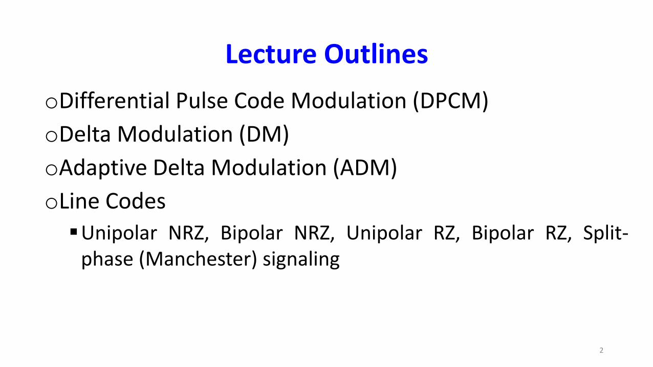
Lecture Outlines

2

oDifferential Pulse Code Modulation (DPCM)

oDelta Modulation (DM)

oAdaptive Delta Modulation (ADM)

oLine Codes

Unipolar NRZ, Bipolar NRZ, Unipolar RZ, Bipolar RZ, Split-phase (Manchester) signaling

Other Types of Digital Pulse Modulation

o Differential Pulse Code Modulation (DPCM) 1-bit DPCM: Delta Modulation (DM)

• Adaptive delta modulation: DM with adaptive step-sizeo Bandwidth-complexity trade-off

An advantage is to lower the bandwidth that is needed to transmit the signal Another advantage is to achieve a cheap and a simple implementation

3

o Unfortunately, we can not achieve both aspects However, based on the system requirements,

we can improve one aspect in the cost ofdegrading the other aspect. How?

Basic Idea for Improving one Performance Aspect in Exchange of Degrading the Other

o We can make a good guess about a sample value from the knowledge of the pastsample values (using a predictor). Why? Sample values are not independent and there is a great deal of redundancy in

the Nyquist sampleso Proper investment of this redundancy lead to:

Encoding a signal with lower number of bits This in turn improves the bandwidth (lower the bandwidth needed for

transmitting the signal) in exchange of increasing the system complexityo Alternatively, increasing this redundancy (e.g., typical DM systems use four time the

Nyquist rate for sampling (oversampling)), increases the bandwidth (degradation) inexchange of the possibility of achieving a simpler and cheaper implementation

4

o Let 𝑘 denote the time instant, 𝑚(𝑘𝑇𝑠) = 𝑚[𝑘] denote the sample value at the timeinstant 𝑘, 𝑇𝑠 denote the sampling interval 𝑇𝑠 = 1/𝑓𝑠.

o Instead of transmitting the signal value 𝑚[𝑘], At the Tx., We transmit the difference between the successive sample values

𝑑 𝑘 = 𝑚 𝑘 −𝑚[𝑘 − 1] 𝑚 𝑘 = 𝑚 𝑘 − 1 for 1-st order predictor, 𝑚 𝑘 is the predicted value of 𝑚 𝑘

At the receiver Rx., we can reconstruct 𝑚[𝑘] from 𝑑[𝑘] and the previous samplevalue (from the knowledge of 𝑑 𝑘 , we can reconstruct 𝑚[𝑘] iteratively at Rx.)

o Since 𝑑[𝑘] is much smaller than 𝑚 𝑘 (quantizing 𝑑[𝑘] needs smaller signal peak

value) and the noise power is:

For a given 𝐿 (or 𝑛), ∆𝑣 is reduced and the noise is reduced, so the SNR increases

For a given SNR, we can reduce 𝑛 (and in turns the transmission bandwidth)

Basic Idea of DPCM: A simple Scheme

5

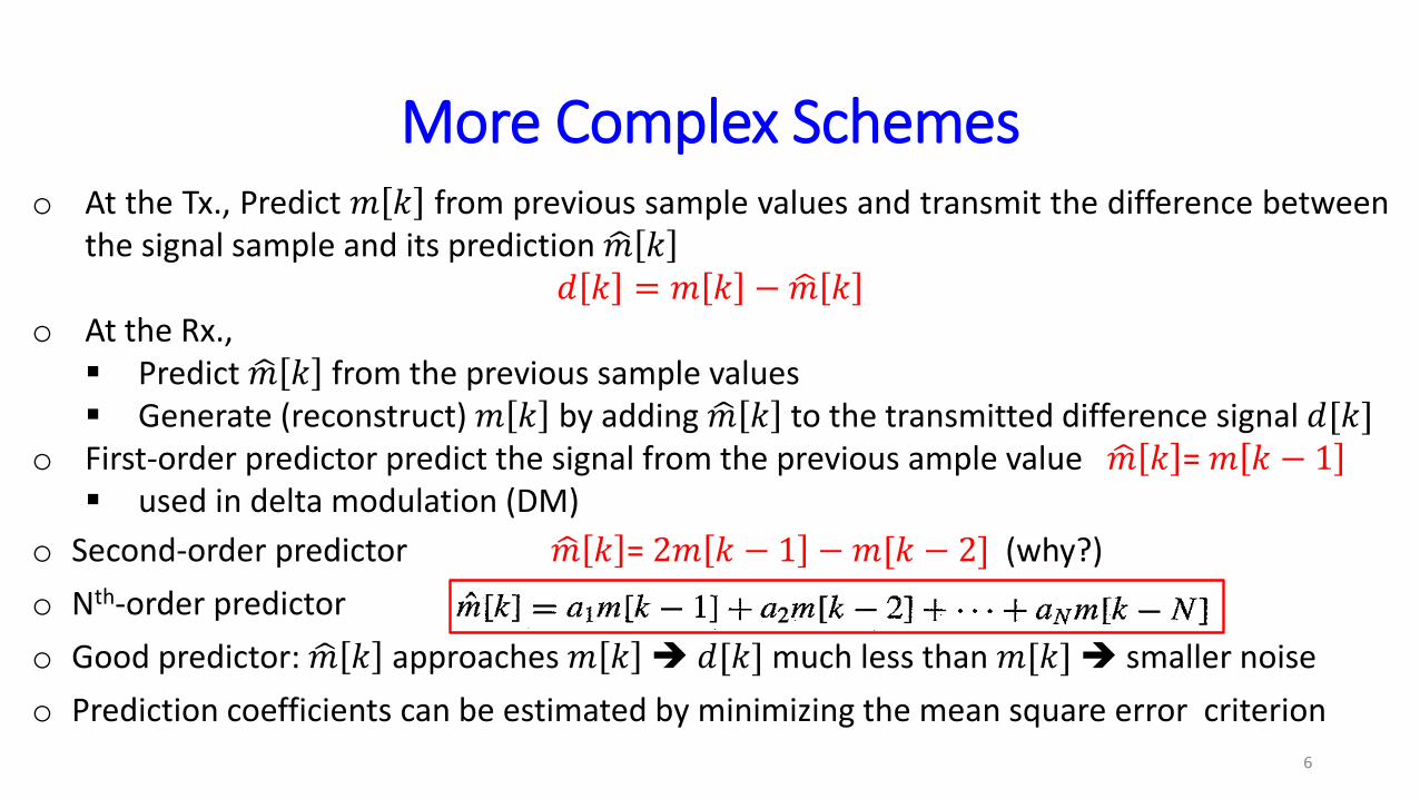
o At the Tx., Predict 𝑚 𝑘 from previous sample values and transmit the difference betweenthe signal sample and its prediction 𝑚 𝑘

𝑑 𝑘 = 𝑚 𝑘 − 𝑚 𝑘o At the Rx.,

Predict 𝑚 𝑘 from the previous sample values Generate (reconstruct) 𝑚 𝑘 by adding 𝑚 𝑘 to the transmitted difference signal 𝑑[𝑘]

o First-order predictor predict the signal from the previous ample value 𝑚 𝑘 = 𝑚 𝑘 − 1 used in delta modulation (DM)

o Second-order predictor 𝑚 𝑘 = 2𝑚 𝑘 − 1 −𝑚[𝑘 − 2] (why?)

o Nth-order predictor

o Good predictor: 𝑚 𝑘 approaches 𝑚 𝑘 𝑑[𝑘] much less than 𝑚[𝑘] smaller noise

o Prediction coefficients can be estimated by minimizing the mean square error criterion

More Complex Schemes

6

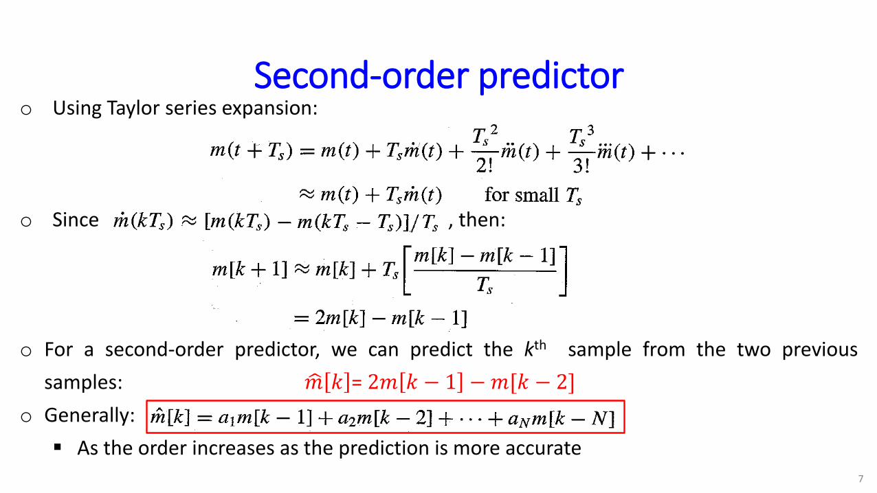
o Using Taylor series expansion:

o Since , then:

o For a second-order predictor, we can predict the kth sample from the two previous

samples: 𝑚 𝑘 = 2𝑚 𝑘 − 1 −𝑚[𝑘 − 2]

o Generally:

As the order increases as the prediction is more accurate

Second-order predictor

7

o Nth-order predictor :

A linear transversal filter achieved using a tapped delay line

Linear Predictor: Transversal Tapped Delay Line Filter

8

a1 a2 aN-1 aN

o If we choose to transmit 𝑑 𝑘 = 𝑚 𝑘 − 𝑚 𝑘 , i.e., before quantizing the signal At the Rx., we face the problem that at the Rx. we do not have the previous samples

𝑚 𝑘 , 𝑚[𝑘 − 1] ,.., otherwise we have the previous quantized samples 𝑚𝑞[𝑘

Which Signal to Transmit, Before or After Quantizing?

9

DPCM System

10

Tx.

Rx.

o Input to predictor 𝑚𝑞 𝑘

o Output of predictor 𝑚𝑞[𝑘] (feedback to its i/p)

o Input to quantizer, the difference 𝑑 𝑘𝑑 𝑘 = 𝑚[𝑘]- 𝑚𝑞[𝑘]

o Output of quantizer, transmitted signal:

𝑑𝑞 𝑘 = 𝑑 𝑘 + 𝑞 𝑘 = 𝑚𝑞[𝑘]- 𝑚𝑞[𝑘]

o Part of the transmitter (shaded area)o Input of channel 𝑑𝑞 𝑘o Output of predictor 𝑚𝑞 𝑘 (same as Tx.)

o Predictor input, receiver output 𝑚𝑞 𝑘

𝑚𝑞 𝑘] = 𝑚 𝑘 + 𝑞[𝑘]

o We are able to receive the desired signalplus a quantization erroro Quantization noise due to 𝑑[𝑘] is much

smaller than of 𝑚[𝑘]o After, the received signal is passed through

a LPF for D/A conversion

SNR Improvement

11

o The noise power is:

o For a given 𝐿 (or 𝑛): ∆𝑣 is reduced and the noise is reduced, so the SNR increases

Let 𝑑𝑝 denote the peak amplitude of the difference signal 𝑑[𝑘]

in PCM 𝑣 = 2𝑚𝑝/𝐿 , where as in DPCM 𝑣 = 2𝑑𝑝/𝐿

𝑣 reduced by a factor 𝑑𝑝/𝑚𝑝 and the noise power 𝑁𝑞 reduced by a factor (𝑑𝑝/𝑚𝑝)2

In additional, the signal power 𝑆𝑜 depends on the square peak value of the signal

assuming that the other statistics are invariant

The SNR improvement (𝐺𝑝) due to prediction is , where 𝑃𝑚 is the power of

𝑚(𝑡) and 𝑃𝑑 is the power of 𝑑(𝑡)

Examples: in practice 𝐺𝑝 can reach 25 dB

o For a given SNR, we can reduce 𝑛 (and in turns the transmission bandwidth)

We can lower 𝑛 of the PCM by 3 or 4 bits/sample (refer to Lathi Book)

Telephone system of DPCM can operate with 32 kbit/sec or even 24 kbit/sec

Delta Modulation (1-bit/sample DPCM)

12

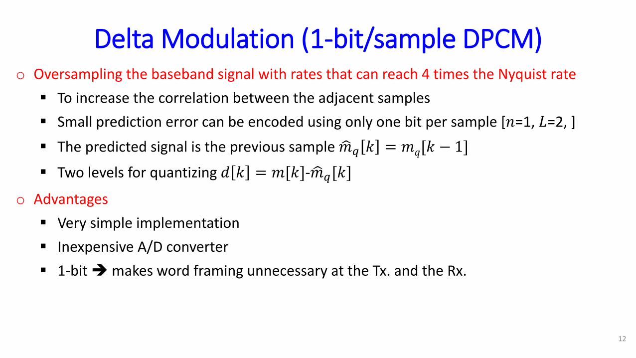
o Oversampling the baseband signal with rates that can reach 4 times the Nyquist rate

To increase the correlation between the adjacent samples

Small prediction error can be encoded using only one bit per sample [𝑛=1, 𝐿=2, ]

The predicted signal is the previous sample 𝑚𝑞 𝑘 = 𝑚𝑞[𝑘 − 1]

Two levels for quantizing 𝑑 𝑘 = 𝑚[𝑘]- 𝑚𝑞[𝑘]

o Advantages

Very simple implementation

Inexpensive A/D converter

1-bitmakes word framing unnecessary at the Tx. and the Rx.

DM Receiver

13

Transmitter

Receiver

o Assuming zero initial condition

First order predictorAdder, accumulator,

integrator

DM System

14

ReceiverTransmitter

o The receiver (demodulator) is just an adder (integrator)

o Integrating of the delta-modulated signal (difference

signal) is an approximation of 𝑚(𝑡)

o The demodulator output 𝑚𝑞 𝑘 when passed through

a low pass filter yields the desired signal reconstructed

from the quantized samples

o The modulator consists of a comparator and a sampler in the

direct pass and an integrator-amplifier in the feedback path

o The analog signal 𝑚(𝑡) is compared with the predicted signal

𝑚𝑞 𝑘

o The error signal 𝑑 𝑘 = 𝑚[𝑘] - 𝑚𝑞 𝑘 𝑖 s applied to a

comparator

If 𝑑 𝑘 > 0 (𝑚 𝑘 > 𝑚𝑞 𝑘 ), o/p=+E otherwise o/p=-E

o The difference 𝑑𝑞 𝑘 is a binary signal (L=2)

o We transmit the derivative of 𝑚 𝑡 , that is 𝑑𝑞 𝑘 : pulse train

Delta Modulating Signal

15

ReceiverTransmitter

16

Illustration of Delta Modulation

Slope Overload Problem of Delta Modulation

17

o Delta modulation faces two problems:

If the variation between the samples is smaller than the step size (𝜎) value (threshold of coding) this variation will

be lost

If he changes are too fast 𝑚𝑞 𝑘 can not follow 𝑚(𝑡) and slope overload occurs

Dynamic operating range is two small due to threshold value and overload effect

o How to overcome the slope overload noise

By increasing the step size problem: this will increase the granular noise (similar to quantization noise)

Granular noise:

Adaptive Delta Modulation (ADM)

18

oUses adaptive step-size according to the level of the input derivative When the slope increases, overload occurs increase the step size during this period

When the slope decrease, reduce the step size reduce the granular noise

Line codes

19

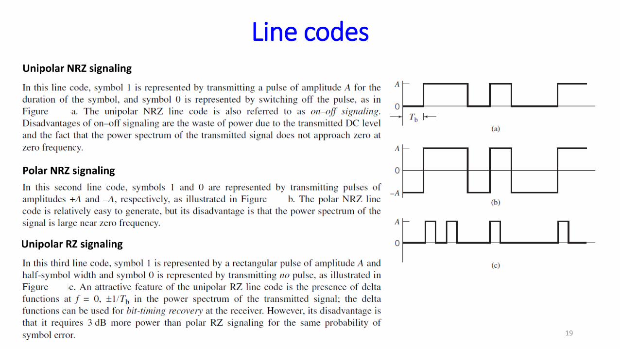
Unipolar NRZ signaling

Polar NRZ signaling

Unipolar RZ signaling

Line codes (Cont’d)

20

(e)

Bipolar RZ signaling

Split Phase (Manchester code)

(e)

Questions

21