1

Abstract

In this study, the evolution of the unsteady trailing edge vortex street downstream a linear turbine cascade is experimentally and computationally investigated. In a transonic cascade test stand, Laser Doppler velocimeter (LDV) measurements were acquired in several axial planes downstream of the blade trailing edge. In addition, direct detection of density changes near the trailing edge provide information about the frequency of a vortex shedding cycle.

A two-dimensional upwind-biased Navier-Stokes solver has then been used to perform a series of steady and unsteady cascade simulations, allowing an in-depth study into the mechanisms of the trailing edge vortex shedding.

The numerical results are compared with the experimental data to test the quality of the numerical simulations. Introduction

Vortex shedding, as excitation for acoustic resonances and structural vibrations, has been an intriguing and challenging flow problem ever since the early works of von Karman on this subject. The literature on vortex shedding from cylinders and flat plates is abundant, but the particular problem of vortex shedding from turbomachinery bladings has received only limited attention (e.g. Sieverding and Heinemann (1990), Cicatelli and Sieverding (1995)).

Nevertheless, the wake flow together with the inherent unsteadiness caused by interaction between stator and rotor has a significant impact on efficiency and performance. Wakes generated by a blade row travel downstream and interact with the succeeding blade rows affecting pressure distribution, heat transfer and boundary layer development. The correct prediction of the wake evolution is necessary for any trust-worthy calculation of blade row interference effects.

Experimental investigations of the far wake mean flow characteristics by means of wake traverse measurements are commonly carried out during turbine cascade testing. Less common are systematic experimental studies of mean velocity and turbulence quantities in the near wake or in the trailing edge region. Even less investigated are the unsteady characteristics of the flow in the wake of turbine cascades in spite of their practical importance and conceptual relevance (Zunino et. al., 1997).

More recently, some experimental studies concentrating on this phenomenon were carried out, e.g. Zunino et. al. (1997) developed a phase locked ensemble averaging technique for separating periodic and random fluctuations and used a triple decomposition to determine the instantaneous velocity to identify periodic organized structures. Cicatelli and Sieverding, 1997 investigated the effect of vortex shedding on the unsteady pressure distribution around the trailing edge of a turbine blade.

Numerical predictions to study the influence of wakes on aerodynamic losses and heat transfer need a correct modeling of wake propagation and wake decay in the axial gap for multi-blade calculations. As e.g. Luo and Lakshminarayana (1997) showed, the prediction of the wake flow depends largely on the turbulence modeling, because it influences blade boundary layers and the wake mixing mechanism. Sondak and Dorney, 1999 simulated vortex shedding in a turbine cascade with a modification to the algebraic Baldwin and Lomax (1978) turbulence model for improved solutions in regions of separated flows and free shear layers and found reasonable good agreement with the experimental pressure data of Cicatelli and Sieverding, 1997. Currie and Carscallen, 1998 used a two equation turbulence model to predict the vortex shedding in a transonic cascade and found that the total pressure loss coefficient predicted by time dependent simulations was significantly higher than the steady state value. These studies indicate, that an unsteady computational approach is necessary to properly capture the complexity of the trailing edge flow.

Investigations of the wake flow downstream of a linear turbine cascade by Sanz et. al., (1998) revealed large discrepancies between LDV-measurement and numerical results, obtained with a two-dimensional upwind-biased Navier-Stokes solver using two different turbulence models. They concluded that a time-accurate computation may be necessary to accurately capture the wake flow field.

The interest of the present contribution is therefore specifically directed towards the investigation of the unsteady trailing edge vortex shedding downstream of a linear turbine cascade by means of an unsteady Navier-Stokes solver and by means of LDV measurements done in several axial planes downstream of the blade trailing edge. In addition, direct detection of density changes near the trailing edge provide information about the frequency of a vortex shedding cycle.

The originality of the present effort can be found in the application of two different turbulence models which are incorporated into an

A.Gehrer, H.Lang, N.Mayrhofer, J.Woisetschläger (2000) Numerical and Experimental Investigation of Trailing Edge Vortex Shedding Downstream of a Linear Turbine Cascade, ASME International Gas Turbine and Aeroengine Congress, Munich, 2000-GT-434

Numerical and Experimental Investigation of Trailing Edge Vortex Shedding Downstream of

a Linear Turbine Cascade

A. Gehrer, H. Lang, N. Mayrhofer, J. Woisetschläger Institute for Thermal Turbomachinery and Machine Dynamics

Technical University of Graz, Austria

2

unsteady Navier-Stokes code, solving the Reynolds-averaged Navier-Stokes equations with an implicit time-marching finite volume method around a two-dimensional blade cascade. A series of steady and unsteady computations has been performed, allowing an in-depth study into the mechanisms of the trailing edge vortex shedding.

The analysis of the results and the comparison with the experimental data will indicate some guideline about the quality of the numerical simulations.

Experimental Facility

The experiment was carried out in a linear cascade wind tunnel capable of supersonic inlet flow which is described in detail by Sanz et al. (1998). The turbine cascade consists of 7 blades as described by Kiock et al. (1986). The most important geometrical characteristics of the blade row and the main flow parameters are summarised in table 1.

Table 1: Blade geometry and flow conditions:

Blade number 7 Chord length 58 mm Axial chord length 48.4 mm Trailing edge thickness 2.9 mm Spacing 41.18 mm Span 100 mm Inlet flow angle 30° Inlet total pressure 1.413 bar Inlet total temperature 308.45 K Isentropic exit Mach number 0.7 Exit Reynolds number 9.75⋅105 Inlet turbulence intensity 5 %

Experimental Setup. Glass windows of 15mm thickness are built in

the side walls to allow optical access to the mid flow passage and to the inlet and exit region. The wake flow downstream of the trailing edge is measured with a Laser-Doppler Velocimeter (LDV). The measurement data in the wake are acquired at midspan at three axial planes located downstream of the cascade at x/cax = 0.037, 0.161 and 0.285 as described by Sanz et al (1998). The first plane is located in the trailing edge region of the wake, where the velocity defect is very large. The other planes are in the near wake region, where the wake defect is still in the order of the mean velocity and where blade geometry and loading are mainly influencing the wake. This classification is made according to Zaccaria and Lakshminarayana (1997). The distance of the third plane corresponds to the rotor-stator spacing of modern axial flow turbines.

For some of the points within the wake, a Polytec laser vibrometer aligned to the LDV measurement volume was used to provide the frequency of the periodic density fluctuations in the wake (Mayrhofer and Woisetschläger , 2000).

To monitor the uniformity of the inlet flow, seven static pressure taps are arranged across two passages at the inlet; two rows of static pressure taps are arranged at the exit. The three middle blades are also equipped with static pressure taps to control the periodicity of the flow, which can be set by a tailboard. From these readings we derived a maximum difference in the isentropic surface Mach number of 0.01, which corresponds to about 1.4%. As pressure sensor we used a Scanivalve ZOC14NP/16Px-50psid calibrated by a dead weight tester to an accuracy of +/- 0.08%. Total pressure and total temperature are measured at the inlet by probes.

The flow conditions in the experiment are subsonic as shown in table 1. The inlet turbulent kinetic energy k of 13.6 m2/s2 corresponds to a turbulence intensity Tu of 5 %.

LDV-Data acquisition and Measurement Accuracy. Experimental data acquisition was done by a two-dimensional LDV system (DANTEC Fiberflow, BSA processors).

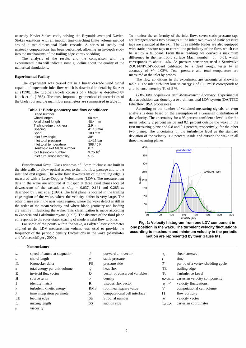
According to the number of validated measuring signals, an error analysis is done based on the assumption of a Gaussian distribution of the velocity. The uncertainty for a 95 percent confidence level is for the mean velocity 2 percent inside and 0.1 percent outside the wake in the first measuring plane and 0.8 and 0.1 percent, respectively, for the other two planes. The uncertainty of the turbulence level as the standard deviation of the velocity is 3 percent inside and outside the wake in all three measuring planes.

80 100 120 140 160 180 200 2200

50

100

150

200

250

300

350

400

velocity [m/s]

coun

ts

periodic RMS

turbulent RMS

Fig. 1: Velocity histogram from one LDV component in one position in the wake. The turbulent velocity fluctuations according to maximum and minimum velocity in the periodic

motion are represented by their Gauss fits.

Nomenclature -

a0 speed of sound at stagnation rn outward unit vector τij shear stresses

c chord length p static pressure t time δij Kronecker delta PS pressure side T period of a vortex shedding cycle e total energy per unit volume &q heat flux TE trailing edge E inviscid flux vector Q vector of conserved variables Tu Turbulence Level H source term ρ density u,v,w,ui cartesian velocity components I identity matrix R viscous flux vector ′ui , ′v velocity fluctuations k turbulent kinetic energy RMS root mean square value V computational cell volume λ time integration parameter S computational cell interface Ω flow vorticity LE leading edge Str Strouhal number

rw velocity vector

lm mixing length SS suction side x,y,z,xi cartesian coordinates μ viscosity

3

80

100

120

140

160

180

200

0 0,1 0,2 0,3 0,4 0,5

Tim e [10-6s]

Velo

city

[m/s

]

s

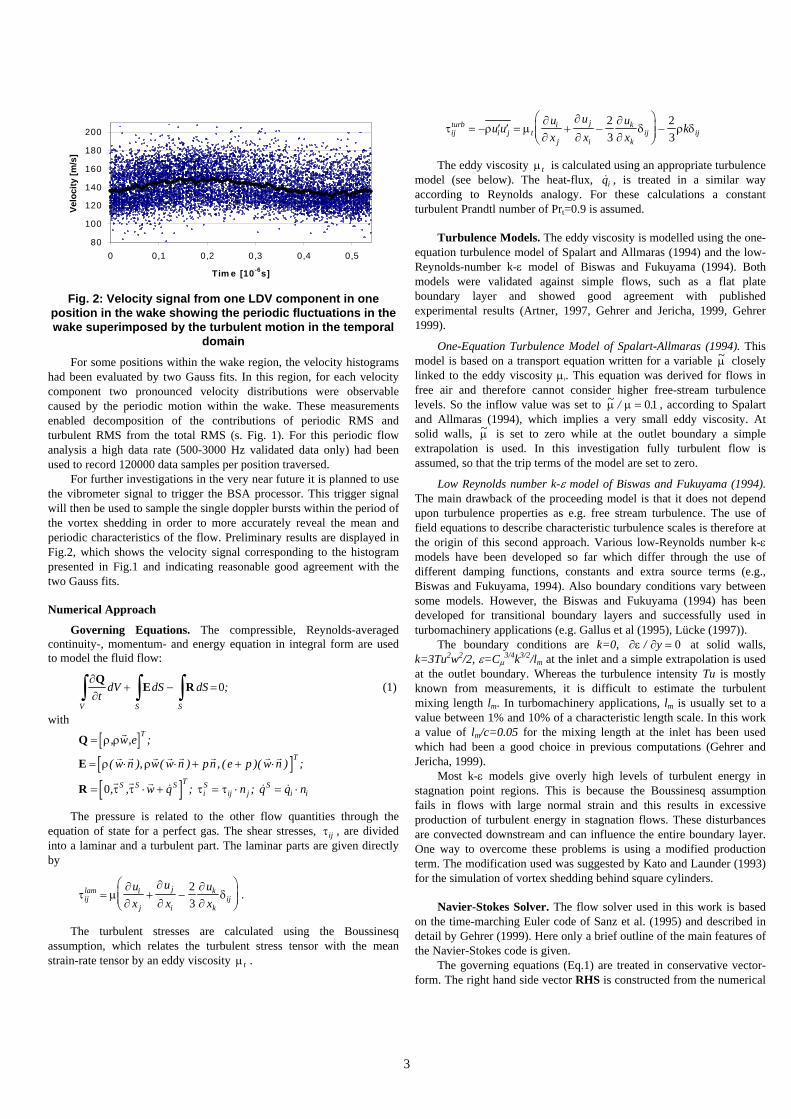
Fig. 2: Velocity signal from one LDV component in one

position in the wake showing the periodic fluctuations in the wake superimposed by the turbulent motion in the temporal

domain

For some positions within the wake region, the velocity histograms had been evaluated by two Gauss fits. In this region, for each velocity component two pronounced velocity distributions were observable caused by the periodic motion within the wake. These measurements enabled decomposition of the contributions of periodic RMS and turbulent RMS from the total RMS (s. Fig. 1). For this periodic flow analysis a high data rate (500-3000 Hz validated data only) had been used to record 120000 data samples per position traversed.

For further investigations in the very near future it is planned to use the vibrometer signal to trigger the BSA processor. This trigger signal will then be used to sample the single doppler bursts within the period of the vortex shedding in order to more accurately reveal the mean and periodic characteristics of the flow. Preliminary results are displayed in Fig.2, which shows the velocity signal corresponding to the histogram presented in Fig.1 and indicating reasonable good agreement with the two Gauss fits. Numerical Approach

Governing Equations. The compressible, Reynolds-averaged continuity-, momentum- and energy equation in integral form are used to model the fluid flow:

∂∂Q

E Rt

dV dS dSV S S∫ ∫ ∫+ − =0; (1)

with

[ ][ ][ ]

Q

E

R

=

= ⋅ ⋅ + + ⋅

= ⋅ + = ⋅ = ⋅

ρ ρ

ρ ρ

τ τ τ τ

, , ;

( ), ( ) , ( )( ) ;

, , & ; ; & &

r

r r r r r r r r

r r r

w e

w n w w n pn e p w n

w q n q q n

T

T

S S S TiS

ij jS

i i0

The pressure is related to the other flow quantities through the equation of state for a perfect gas. The shear stresses, τij , are divided into a laminar and a turbulent part. The laminar parts are given directly by

τ μ∂∂

∂

∂∂∂

δijlam i

j

j

i

k

kij

ux

ux

ux

= + −⎛

⎝⎜⎜

⎞

⎠⎟⎟

23

.

The turbulent stresses are calculated using the Boussinesq assumption, which relates the turbulent stress tensor with the mean strain-rate tensor by an eddy viscosity μt .

τ ρ μ∂∂

∂

∂∂∂

δ ρ δijturb

i j ti

j

j

i

k

kij iju u

ux

ux

ux

k= − ′ ′ = + −⎛

⎝⎜⎜

⎞

⎠⎟⎟ −

23

23

The eddy viscosity μt is calculated using an appropriate turbulence model (see below). The heat-flux, &qi , is treated in a similar way according to Reynolds analogy. For these calculations a constant turbulent Prandtl number of Prt=0.9 is assumed.

Turbulence Models. The eddy viscosity is modelled using the one-equation turbulence model of Spalart and Allmaras (1994) and the low-Reynolds-number k-ε model of Biswas and Fukuyama (1994). Both models were validated against simple flows, such as a flat plate boundary layer and showed good agreement with published experimental results (Artner, 1997, Gehrer and Jericha, 1999, Gehrer 1999).

One-Equation Turbulence Model of Spalart-Allmaras (1994). This model is based on a transport equation written for a variable ~μ closely linked to the eddy viscosity μt. This equation was derived for flows in free air and therefore cannot consider higher free-stream turbulence levels. So the inflow value was set to ~ / .μ μ = 01 , according to Spalart and Allmaras (1994), which implies a very small eddy viscosity. At solid walls, ~μ is set to zero while at the outlet boundary a simple extrapolation is used. In this investigation fully turbulent flow is assumed, so that the trip terms of the model are set to zero.

Low Reynolds number k-ε model of Biswas and Fukuyama (1994). The main drawback of the proceeding model is that it does not depend upon turbulence properties as e.g. free stream turbulence. The use of field equations to describe characteristic turbulence scales is therefore at the origin of this second approach. Various low-Reynolds number k-ε models have been developed so far which differ through the use of different damping functions, constants and extra source terms (e.g., Biswas and Fukuyama, 1994). Also boundary conditions vary between some models. However, the Biswas and Fukuyama (1994) has been developed for transitional boundary layers and successfully used in turbomachinery applications (e.g. Gallus et al (1995), Lücke (1997)).

The boundary conditions are k=0, ∂ε ∂/ y = 0 at solid walls, k=3Tu2w2/2, ε=Cμ

3/4k3/2/lm at the inlet and a simple extrapolation is used at the outlet boundary. Whereas the turbulence intensity Tu is mostly known from measurements, it is difficult to estimate the turbulent mixing length lm. In turbomachinery applications, lm is usually set to a value between 1% and 10% of a characteristic length scale. In this work a value of lm/c=0.05 for the mixing length at the inlet has been used which had been a good choice in previous computations (Gehrer and Jericha, 1999).

Most k-ε models give overly high levels of turbulent energy in stagnation point regions. This is because the Boussinesq assumption fails in flows with large normal strain and this results in excessive production of turbulent energy in stagnation flows. These disturbances are convected downstream and can influence the entire boundary layer. One way to overcome these problems is using a modified production term. The modification used was suggested by Kato and Launder (1993) for the simulation of vortex shedding behind square cylinders.

Navier-Stokes Solver. The flow solver used in this work is based on the time-marching Euler code of Sanz et al. (1995) and described in detail by Gehrer (1999). Here only a brief outline of the main features of the Navier-Stokes code is given.

The governing equations (Eq.1) are treated in conservative vector-form. The right hand side vector RHS is constructed from the numerical

4

approximation for the source term H, present only in the turbulence models, and the representative Fluxes at the bounding sides of the cell are given by E+1/2, R+1/2, which approximate the real Fluxes ∫EdS, ∫RdS to the required order of accuracy.

∂∂Q

RHSt= (2)

( ) ( )RHS H E E R R= − − − −⎡⎣⎢

⎤⎦⎥+ − + −∑ ∑$ $ $ $ $

/ / / /1

1 2 1 2 1 2 1 2V

Implicit Time-Integration. Eq.2 is discretized in time by applying an implicit method leading to a set of non-linear finite difference equations:

( )Q Q

RHS RHSn n

n n

t

++−

= ⋅ + − ⋅1

1 1Δ

λ λ (3)

To obtain time-accurate solutions at each time level, inner iterations, so called Newton iterations, are introduced. Solving Eq.3, using a Newton procedure, can be described by:

( )

( )

IRHS

QQ Q Q

RHS RHS

−⎛⎝⎜

⎞⎠⎟

⎛

⎝⎜⎜

⎞

⎠⎟⎟ = − −

+ ⋅ + − ⋅

λ∂∂

λ λ

Δ Δ

Δ Δ

t

t t

pp p n

p n1

(4)

where p denotes a subiteration index and λ is a time-integration parameter which enables a blending between the first-order accurate, fully-implicit Euler backward scheme (λ=1) and the second-order accurate time-centred implicit trapezoidal method (λ=0.5).

In stationary simulations convergence is optimised by using a local time step based on a local stability criterion and in addition, by applying a multigrid procedure based on Jameson and Yoon (1986) and Siikonen (1991).

Inviscid Fluxes. The convective (Euler) parts $E , $ESA , $Ekε are discretized using a third-order-accurate, TVD-upwind, cell-centred finite volume scheme, based on Roe's approximate Riemann solver (Roe, 1981, Sanz et al., 1995). For the time linearization of the convective flux vector only a first order accurate upwind-scheme is considered.

Viscous Fluxes. In order to construct the numerical viscous flux vector at the cell interfaces $R , $R SA , $R kε , it is necessary to evaluate first-order derivatives of the velocity components, the speed of sound and the turbulent quantities, which is done in a central-differencing manner, using Green's theorem (e.g., Furukawa et al. 1991). The time linearization of the viscous flux vector is performed by applying the thin-layer approximation for the implicit side of the equations.

Source Terms. The source terms $HSA , $Hkε are evaluated as cell averages. To estimate the gradients present in the source terms, a cell-centred finite volume scheme is used. This gives a second-order accurate estimation of the gradients. For the implicit side of the equations, a true linearization of the source terms is performed.

Boundary Conditions. In the present cell-centred scheme, phantom cells are used to handle all boundaries. According to the theory of characteristics, flow angle, total pressure, total temperature and isentropic relations are used at the subsonic axial inlet, whereas all variables are prescribed at the supersonic inlet. At the subsonic axial outlet the average value of the static pressure is prescribed, density and velocity components are extrapolated, whereas all variables are extrapolated at supersonic axial outlet. On solid walls, the pressure is extrapolated from the interior points and the non-slip adiabatic or isothermal condition is used to compute density and total energy.

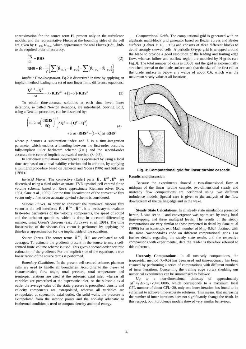
Computational Grids. The computational grid is generated with an algebraic multi-block grid generator based on Bézier curves and Bézier surfaces (Gehrer et al., 1996) and consists of three different blocks to avoid strongly skewed cells. A periodic O-type grid is wrapped around the blade to provide a good resolution of the leading and trailing edge flow, whereas inflow and outflow region are modeled by H-grids (see Fig.3). The total number of cells is 18688 and the grid is exponentially stretched normal to the blade surface such that the size of the first cell at the blade surface is below a y+-value of about 0.6, which was the maximum steady value at all locations.

Fig. 3: Computational grid for linear turbine cascade

Results and discussion

Because the experiments showed a two-dimensional flow at midspan of the linear turbine cascade, two-dimensional steady and unsteady flow computations are performed using two different turbulence models. Special care is given to the analysis of the flow downstream of the trailing edge and in the wake.

Steady State Calculations. In all steady state simulations presented

herein, λ was set to 1 and convergence was optimised by using local time-stepping and three multigrid levels. The results of the steady computations are very similar to those presented in detail by Sanz et. al (1998) for an isentropic exit Mach number of M2,is=0.624 obtained with the same Navier-Stokes code on different computational grids. For further details regarding the steady state results and the respective comparisons with experimental, data the reader is therefore referred to this reference.

Unsteady Computations. In all unsteady computations, the

trapezoidal method (λ=0.5) has been used and time-accuracy has been ensured by performing a series of computations with different numbers of inner iterations. Concerning the trailing edge vortex shedding our numerical experiments can be summarised as follows:

Up to a non-dimensional timestep of approximately Δt* = ( / )Δt a c⋅ 0 =0.0006, which corresponds to a maximum local CFL-number of about CFL=20, only one inner iteration has found to be sufficient to achieve time-accurate solutions. This means, that increasing the number of inner iterations does not significantly change the result. In this respect, both turbulence models showed very similar behaviour.

5

It should also be noted that when choosing larger timesteps, one has to appropriately increase the number of inner iterations (e.g. Furukawa et al., 1992), what has turned out to be less efficient (in terms of computational time) in this case.

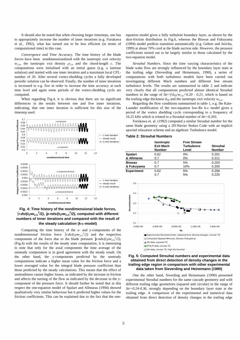
Convergence and Time Accuracy. The time history of the blade forces have been nondimensionalized with the isentropic exit velocity w2,is, the isentropic exit density ρ2,is and the chord-length c. The computations were initialised with an initial guess (e.g. a laminar solution) and started with one inner iteration and a maximum local CFL-number of 20. After several vortex-shedding cycles a fully developed periodic solution can be observed. Finally, the number of inner iterations is increased to e.g. five in order to increase the time accuracy at each time level and again some periods of the vortex-shedding cycle are computed.

When regarding Fig.4, it is obvious that there are no significant differences in the results between one and five inner iterations, indicating, that one inner iteration is sufficient for this size of the timestep used.

0.50.520.540.560.58

0.60.620.640.660.68

0.7

0 2 4 6 8 10 12 14

nondimensional time

Inte

gral

Pre

ssur

e C

oeffi

cien

t

1 inner iterationsteady result5 inner iterations

x-component

y-component

0.0020.00220.00240.00260.0028

0.0030.00320.00340.00360.0038

0 2 4 6 8 10 12 14

nondimensional time

Inte

gral

Fric

tion

Coe

ffici

ent

1 inner iterationsteady result5 inner iterations

x-component (friction)

y-component (friction)

Fig. 4: Time history of the nondimensional blade forces,

∫τ⋅ds/(cρw2,is2/2), ∫p⋅nds/(cρw2,is

2/2), computed with different numbers of inner iterations and compared with the result of

the steady calculation (k-ε-model)

Comparing the time history of the x- and y-components of the nondimensional friction force ∫τ⋅ds/(cρw2,is

2/2) and the respective components of the force due to the blade pressure ∫p⋅nds/(cρw2,is

2/2), (Fig.4) with the results of the steady state computation, it is interesting to note that only for the axial components the time average of the unsteady computation is in good agreement with the steady result. On the other hand, the y-components predicted by the unsteady computations indicate a higher mean value for the friction force and a lower averaged value for the integral blade pressure coefficient than those predicted by the steady calculations. This means that the effect of unsteadiness causes higher losses, as indicated by the increase in friction and affects the turning of the flow as indicated by the decrease in the y-component of the pressure force. It should further be noted that in this respect the one-equation model of Spalart and Allmaras (1994) showed qualitatively very similar behaviour but it predicted higher values for the friction coefficients. This can be explained due to the fact that the one-

equation model gives a fully turbulent boundary layer, as shown by the skin-friction distribution in Fig.6, whereas the Biswas and Fukuyama (1994) model predicts transition automatically (e.g. Gehrer and Jericha, 1999) at about 70% cord at the blade suction side. However, the pressure coefficients turned out to be largely similar to those calculated by the two-equation model.

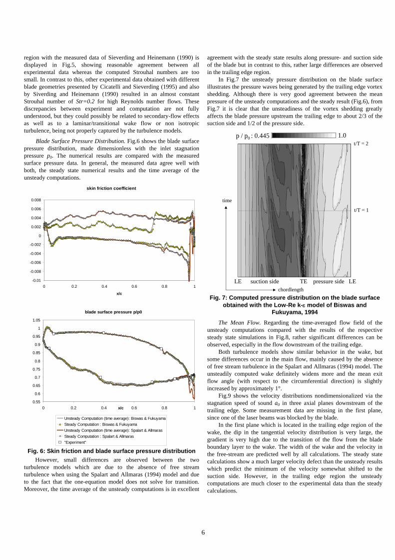
Strouhal Numbers. Since the time varying characteristics of the blade wake flow are strongly influenced by the boundary layer state at the trailing edge (Sieverding and Heinemann, 1990), a series of computations with both turbulence models have been carried out investigating different Mach numbers and different free stream turbulence levels. The results are summarised in table 2 and indicate very clearly that all computations predicted almost identical Strouhal numbers in the range of Str=f⋅dTE/w2,is=0.20 - 0.21, which is based on the trailing edge thickness dTE and the isentropic exit velocity w2,is.

Regarding the flow conditions summarised in table 1, e.g. the Kato-Launder modification of the two-equation low-Re k-ε model gives a period of the vortex shedding cycle corresponding to a frequency of 16.25 kHz which is related to a Strouhal number of Str=0.203.

Furukawa et. al. (1992) computed a similar Strouhal number for the same blade geometry using a 2D-Navier Stokes Code with an implicit upwind relaxation scheme and an algebraic Turbulence model.

Table 2: Strouhal Numbers

Isentropic Free Stream Exit Mach Turbulence Strouhal Number Level Number Spalart 0.62 0% 0.201 & Allmaras 0.7 0% 0.211 Biswas 0.7 5% 0.203 & Fukuyama 0.7 10% 0.200 Experiment 0.62 5% 0.256 0.7 5% 0.225

0.1

0.2

0.3

0.4

0.5

0.00E+00 4.00E+05 8.00E+05 1.20E+06 1.60E+06

Re

Stro

uhal

num

ber

Experimental Strouhalnumber, obtained from density changes, circular TEComputed (Spalart-Allmaras, Biswas-Fukuyama)

VKI-data, squared TE

DFVLR-data, circular TEVKI-data, circular TE, High Re-Number

Fig. 5: Computed Strouhal numbers and experimental data

obtained from direct detection of density changes in the trailing edge region in comparison with other experimental

data taken from Sieverding and Heinemann (1990)

One the other hand, Siverding and Heinemann (1990) presented experimental Strouhal numbers for the same cascade geometry and with different trailing edge geometries (squared and circular) in the range of Str=0.24-0.36, strongly depending on the boundary layer state at the trailing edge. A comparison of the experimental and numerical data obtained from direct detection of density changes in the trailing edge

6

region with the measured data of Sieverding and Heinemann (1990) is displayed in Fig.5, showing reasonable agreement between all experimental data whereas the computed Strouhal numbers are too small. In contrast to this, other experimental data obtained with different blade geometries presented by Cicatelli and Sieverding (1995) and also by Siverding and Heinemann (1990) resulted in an almost constant Strouhal number of Str=0.2 for high Reynolds number flows. These discrepancies between experiment and computation are not fully understood, but they could possibly be related to secondary-flow effects as well as to a laminar/transitional wake flow or non isotropic turbulence, being not properly captured by the turbulence models.

Blade Surface Pressure Distribution. Fig.6 shows the blade surface pressure distribution, made dimensionless with the inlet stagnation pressure p0. The numerical results are compared with the measured surface pressure data. In general, the measured data agree well with both, the steady state numerical results and the time average of the unsteady computations.

skin friction coefficient

-0.01

-0.008

-0.006

-0.004

-0.002

0

0.002

0.004

0.006

0.008

0 0.2 0.4 0.6 0.8 1

x/c

blade surface pressure p/p0

0.55

0.6

0.65

0.7

0.75

0.8

0.85

0.9

0.95

1

1.05

0 0.2 0.4 0.6 0.8 1x/c

Unsteady Computation (time average): Biswas & FukuyamaSteady Computation : Biswas & FukuyamaUnsteady Computation (time average): Spalart & AllmarasSteady Computation : Spalart & Allmaras"Experiment"

Fig. 6: Skin friction and blade surface pressure distribution

However, small differences are observed between the two turbulence models which are due to the absence of free stream turbulence when using the Spalart and Allmaras (1994) model and due to the fact that the one-equation model does not solve for transition. Moreover, the time average of the unsteady computations is in excellent

agreement with the steady state results along pressure- and suction side of the blade but in contrast to this, rather large differences are observed in the trailing edge region.

In Fig.7 the unsteady pressure distribution on the blade surface illustrates the pressure waves being generated by the trailing edge vortex shedding. Although there is very good agreement between the mean pressure of the unsteady computations and the steady result (Fig.6), from Fig.7 it is clear that the unsteadiness of the vortex shedding greatly affects the blade pressure upstream the trailing edge to about 2/3 of the suction side and 1/2 of the pressure side.

p / p0 : 0.445 1.0

LE suction side TE pressure side LEchordlength

time

t/T = 1

t/T = 2

Fig. 7: Computed pressure distribution on the blade surface obtained with the Low-Re k-ε model of Biswas and

Fukuyama, 1994

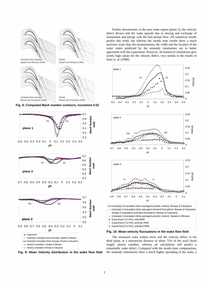
The Mean Flow. Regarding the time-averaged flow field of the unsteady computations compared with the results of the respective steady state simulations in Fig.8, rather significant differences can be observed, especially in the flow downstream of the trailing edge.

Both turbulence models show similar behavior in the wake, but some differences occur in the main flow, mainly caused by the absence of free stream turbulence in the Spalart and Allmaras (1994) model. The unsteadily computed wake definitely widens more and the mean exit flow angle (with respect to the circumferential direction) is slightly increased by approximately 1°.

Fig.9 shows the velocity distributions nondimensionalized via the stagnation speed of sound a0 in three axial planes downstream of the trailing edge. Some measurement data are missing in the first plane, since one of the laser beams was blocked by the blade.

In the first plane which is located in the trailing edge region of the wake, the dip in the tangential velocity distribution is very large, the gradient is very high due to the transition of the flow from the blade boundary layer to the wake. The width of the wake and the velocity in the free-stream are predicted well by all calculations. The steady state calculations show a much larger velocity defect than the unsteady results which predict the minimum of the velocity somewhat shifted to the suction side. However, in the trailing edge region the unsteady computations are much closer to the experimental data than the steady calculations.

7

Spalart and Allmaras (1994) Spalart and Allmaras (1994)

Biswas and Fukuyama (1994) Biswas and Fukuyama (1994)

Unsteady (time average)

Unsteady (time average) Steady

Steady

Fig. 8: Computed Mach number contours, increment 0.02

plane 1

0.2

0.3

0.4

0.5

0.6

0.7

-0.5 -0.4 -0.3 -0.2 -0.1 0 0.1 0.2 0.3 0.4 0.5y/t

Mac

h N

umbe

r w

/a0PS SS

plane 2

0.20.30.40.50.60.7

-0.7 -0.6 -0.5 -0.4 -0.3 -0.2 -0.1 0 0.1 0.2 0.3y/t

Mac

h N

umbe

r w

/a0PS SS

plane 30.2

0.3

0.4

0.5

0.6

0.7

-0.9 -0.8 -0.7 -0.6 -0.5 -0.4 -0.3 -0.2 -0.1 0 0.1y/t

Mac

h N

umbe

r w

/a0

ExperimentUnsteady Computation (time-average): Spalart & AllmarasUnsteady Computation (time-average): Biswas & FukuyamaSteady Computation : Spalart & AllmarasSteady Computation: Biswas & Fukuyama

PS SS

Fig. 9: Mean Velocity distribution in the wake flow field

Further downstream, in the near wake region (plane 2), the velocity defect decays and the wake spreads due to mixing and exchange of momentum and energy with the free-stream flow. All numerical results predict this trend, but whereas the steady state results show a much narrower wake than the measurements, the width and the location of the wake centre predicted by the unsteady simulations are in better agreement with the experiment. However, all numerical simulations give overly high values for the velocity defect, very similar to the results of Sanz et. al. (1998).

plane 1

0

0.05

0.1

0.15

0.2

0.25

-0.5 -0.4 -0.3 -0.2 -0.1 0 0.1 0.2 0.3 0.4 0.5

y/t

RM

S/a

0SSPS

plane 2

0

0.05

0.1

0.15

0.2

0.25

-0.7 -0.6 -0.5 -0.4 -0.3 -0.2 -0.1 0 0.1 0.2 0.3

y/t

RM

S/a

0

SSPS

plane 3

0

0.05

0.1

0.15

0.2

0.25

-0.9 -0.8 -0.7 -0.6 -0.5 -0.4 -0.3 -0.2 -0.1 0 0.1

y/t

RM

S/a

0

Unsteady Computation (time-averaged periodic motion): Biswas & FukuyamaUnsteady Computation (time-averaged turbulent fluctuation): Biswas & FukuyamaSteady Computation (turbulent fluctuation): Biswas & FukuyamaUnsteady Computation (time-averaged periodic motion): Spalart & AllmarasExperiment (Tu=5%), total RMSExperiment (Tu=5%), periodic RMSExperiment (Tu=5%), turbulent RMS

SSPS

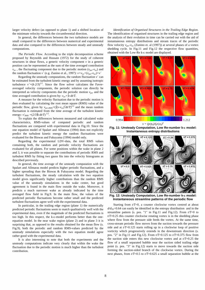
Fig. 10: Mean velocity fluctuations in the wake flow field

The measured wake widens more and the velocity defect in the third plane, at a streamwise distance of about 75% of the axial chord length, almost vanishes, whereas all calculations still predict a remarkable wake defect. Compared with the steady-state computations, the unsteady simulations show a much higher spreading of the wake, a

8

larger velocity defect (as opposed to plane 1) and a shifted location of the minimum velocity towards the circumferential direction.

In general, the differences between the two turbulence models are small compared to the differences between numerical and experimental data and also compared to the differences between steady and unsteady computations.

The Periodic Flow. According to the triple decomposition scheme proposed by Reynolds and Hussain (1972) for the study of coherent structures in shear flows, a generic velocity component v in a generic position can be represented as the sum of the time averaged contribution vav , the fluctuating component due to the periodic motion (vper-vav) and the random fluctuation v´ (e.g. Zunino et al., 1997): v=vav+(vper-vav)+v´

Regarding the unsteady computations, the random fluctuation v´ can be estimated from the turbulent kinetic energy and by assuming isotropic turbulence v´=(k⋅2/3)1/2. Since the flow solver calculates the Favre-averaged velocity components, the periodic solution can directly be interpreted as velocity components due the periodic motion vper and the time averaged contribution is given by: vav=∫v⋅dt/T.

A measure for the velocity fluctuation due to the periodic motion is then evaluated by calculating the root mean square (RMS) value of the periodic flow, given by vper,RMS=(∫(v-vav)2dt/T)1/2 and the mean random fluctuation is estimated from the time average of the turbulent kinetic energy: v'RMS =(2/3∫k⋅dt/T) 1/2.

To explain the differences between measured and calculated wake characteristics, RMS-values of computed periodic and random fluctuations are compared with experimental data in Fig.10. Since the one equation model of Spalart and Allmaras (1994) does not explicitly predict the turbulent kinetic energy the random fluctuations were evaluated for the Biswas and Fukuyama (1994) model only.

Regarding the experimental LDV-data, the total RMS values containing both, the random and periodic velocity fluctuations are evaluated for all planes. For some positions within the wake in plane 2 and 3, it was possible to separate the contributions of periodic RMS and turbulent RMS by fitting two gauss fits into the velocity histograms as described previously.

In general, the time average of the unsteady computation with the Spalart and Allmaras model predicts higher periodic fluctuations, and a higher spreading than the Biswas & Fukuyama model. Regarding the turbulent fluctuations, the steady calculation with the two equation model gives significantly higher contributions than the random RMS value of the unsteady simulations in the wake center, but good agreement is found in the main flow outside the wake. Moreover, it predicts a much narrower wake as already indicated by the time averaged flow field in Fig.9. In the main flow, the values of the predicted periodic fluctuations become rather small and the predicted turbulent fluctuations agree well with the experimental data.

In particular, in the trailing edge region (plane 1) the numerically predicted periodic fluctuations seem to match qualitatively well with the experimental data, even if the magnitude of the predicted fluctuations is too high. In this respect, the k-ε-model performs better than the one-equation model. In the near wake region (plane 2) and in plane 3 it is surprising that, as opposed to the results obtained for the mean flow (s. Fig.9), both the periodic and random RMS-values predicted by the unsteady simulations especially with the two equation model agree rather good with the experimental data.

It is also interesting to note that both the experiments and the unsteady computations indicate very clearly that within the wake the fluctuation due to the periodic motion is much higher than the turbulent contribution.

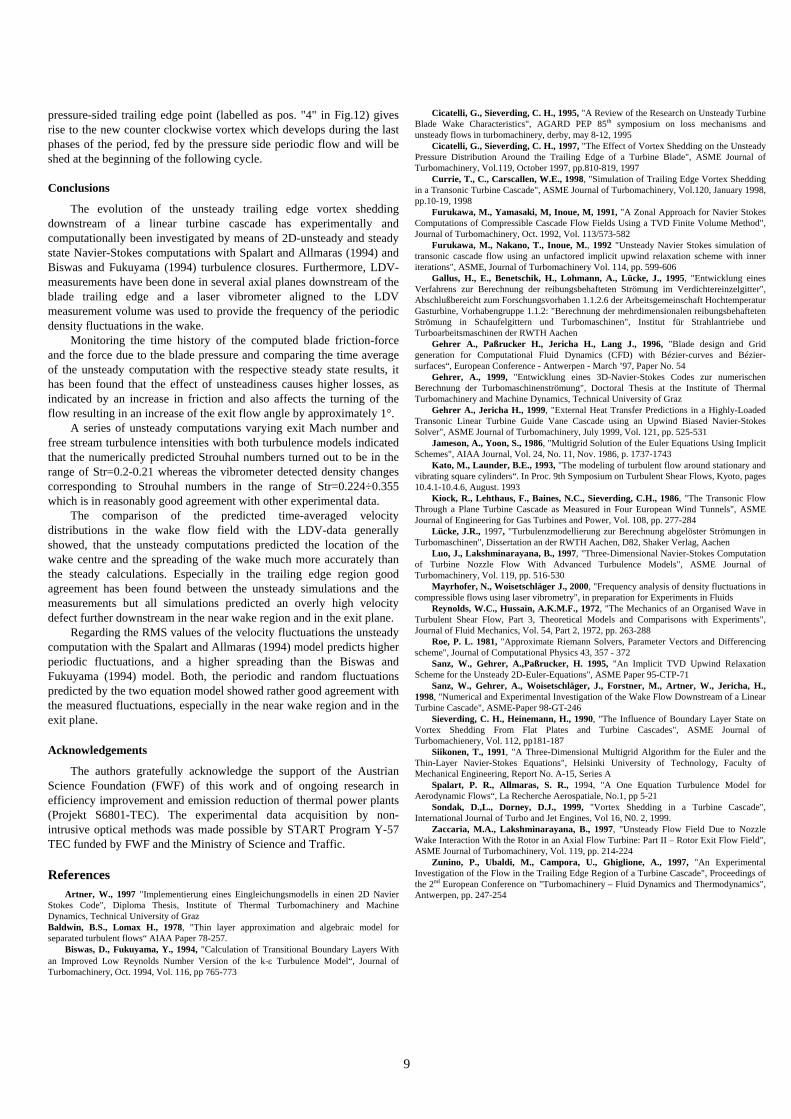
Identification of Organised Structures in the Trailing Edge Region. The identification of organised structures in the trailing edge region and the analysis of their evolution in time can be carried out with the aid of instantaneous entropy distributions and stream traces of the periodic flow velocity vper-vav (Zunino et. al (1997)) at several phases of a vortex shedding cycle. In Fig.11 and Fig.12 the respective flow quantities, obtained with the Low-Re k-ε model are displayed.

0.994 1.212 s = (p/p0)/(ρ/ρ0)κ

Fig. 11: Unsteady Computation, Low Re-number k-ε model: Instantaneous entropy distributions

Fig. 12: Unsteady Computation, Low Re-number k-ε model: Instantaneous streamline patterns of the periodic flow

Starting from t/T=0, a counter clockwise vortex centred at about d/dTE=0.64 can easily be identified in the entropy distribution and in the streamline pattern (s. pos. "1" in Fig.11 and Fig.12). From t/T=0 to t/T=0.25 this counter clockwise rotating vortex is in the shedding phase where flow from the pressure side feeds the vortex. At the same time, cross-stream periodic flow moves from the suction towards the pressure side and at t/T=0.125 starts rolling up in a clockwise loop of positive vorticity which progressively extends in the downstream direction (s. pos. "2" in Fig.11 and Fig.12). From t/T=0.125 to t/T=0.375 flow from the suction side enters this new clockwise vortex and at t/T=0.25 the flow of a small separated bubble near the suction sided trailing edge point (s. pos. "3" in Fig.12) starts to move towards the suction side forming the suction-sided branch of the clockwise vortex. During the next phases, from t/T=0.5 to t/T=0.625 a small separation bubble at the

9

pressure-sided trailing edge point (labelled as pos. "4" in Fig.12) gives rise to the new counter clockwise vortex which develops during the last phases of the period, fed by the pressure side periodic flow and will be shed at the beginning of the following cycle. Conclusions

The evolution of the unsteady trailing edge vortex shedding downstream of a linear turbine cascade has experimentally and computationally been investigated by means of 2D-unsteady and steady state Navier-Stokes computations with Spalart and Allmaras (1994) and Biswas and Fukuyama (1994) turbulence closures. Furthermore, LDV-measurements have been done in several axial planes downstream of the blade trailing edge and a laser vibrometer aligned to the LDV measurement volume was used to provide the frequency of the periodic density fluctuations in the wake.

Monitoring the time history of the computed blade friction-force and the force due to the blade pressure and comparing the time average of the unsteady computation with the respective steady state results, it has been found that the effect of unsteadiness causes higher losses, as indicated by an increase in friction and also affects the turning of the flow resulting in an increase of the exit flow angle by approximately 1°.

A series of unsteady computations varying exit Mach number and free stream turbulence intensities with both turbulence models indicated that the numerically predicted Strouhal numbers turned out to be in the range of Str=0.2-0.21 whereas the vibrometer detected density changes corresponding to Strouhal numbers in the range of Str=0.224÷0.355 which is in reasonably good agreement with other experimental data.

The comparison of the predicted time-averaged velocity distributions in the wake flow field with the LDV-data generally showed, that the unsteady computations predicted the location of the wake centre and the spreading of the wake much more accurately than the steady calculations. Especially in the trailing edge region good agreement has been found between the unsteady simulations and the measurements but all simulations predicted an overly high velocity defect further downstream in the near wake region and in the exit plane.

Regarding the RMS values of the velocity fluctuations the unsteady computation with the Spalart and Allmaras (1994) model predicts higher periodic fluctuations, and a higher spreading than the Biswas and Fukuyama (1994) model. Both, the periodic and random fluctuations predicted by the two equation model showed rather good agreement with the measured fluctuations, especially in the near wake region and in the exit plane. Acknowledgements

The authors gratefully acknowledge the support of the Austrian Science Foundation (FWF) of this work and of ongoing research in efficiency improvement and emission reduction of thermal power plants (Projekt S6801-TEC). The experimental data acquisition by non-intrusive optical methods was made possible by START Program Y-57 TEC funded by FWF and the Ministry of Science and Traffic. References

Artner, W., 1997 "Implementierung eines Eingleichungsmodells in einen 2D Navier Stokes Code", Diploma Thesis, Institute of Thermal Turbomachinery and Machine Dynamics, Technical University of Graz Baldwin, B.S., Lomax H., 1978, "Thin layer approximation and algebraic model for separated turbulent flows“ AIAA Paper 78-257.

Biswas, D., Fukuyama, Y., 1994, "Calculation of Transitional Boundary Layers With an Improved Low Reynolds Number Version of the k-ε Turbulence Model“, Journal of Turbomachinery, Oct. 1994, Vol. 116, pp 765-773

Cicatelli, G., Sieverding, C. H., 1995, "A Review of the Research on Unsteady Turbine Blade Wake Characteristics", AGARD PEP 85th symposium on loss mechanisms and unsteady flows in turbomachinery, derby, may 8-12, 1995

Cicatelli, G., Sieverding, C. H., 1997, "The Effect of Vortex Shedding on the Unsteady Pressure Distribution Around the Trailing Edge of a Turbine Blade", ASME Journal of Turbomachinery, Vol.119, October 1997, pp.810-819, 1997

Currie, T., C., Carscallen, W.E., 1998, "Simulation of Trailing Edge Vortex Shedding in a Transonic Turbine Cascade", ASME Journal of Turbomachinery, Vol.120, January 1998, pp.10-19, 1998

Furukawa, M., Yamasaki, M, Inoue, M, 1991, "A Zonal Approach for Navier Stokes Computations of Compressible Cascade Flow Fields Using a TVD Finite Volume Method", Journal of Turbomachinery, Oct. 1992, Vol. 113/573-582

Furukawa, M., Nakano, T., Inoue, M., 1992 "Unsteady Navier Stokes simulation of transonic cascade flow using an unfactored implicit upwind relaxation scheme with inner iterations", ASME, Journal of Turbomachinery Vol. 114, pp. 599-606

Gallus, H., E., Benetschik, H., Lohmann, A., Lücke, J., 1995, "Entwicklung eines Verfahrens zur Berechnung der reibungsbehafteten Strömung im Verdichtereinzelgitter", Abschlußbereicht zum Forschungsvorhaben 1.1.2.6 der Arbeitsgemeinschaft Hochtemperatur Gasturbine, Vorhabengruppe 1.1.2: "Berechnung der mehrdimensionalen reibungsbehafteten Strömung in Schaufelgittern und Turbomaschinen", Institut für Strahlantriebe und Turboarbeitsmaschinen der RWTH Aachen

Gehrer A., Paßrucker H., Jericha H., Lang J., 1996, "Blade design and Grid generation for Computational Fluid Dynamics (CFD) with Bézier-curves and Bézier-surfaces“, European Conference - Antwerpen - March ’97, Paper No. 54

Gehrer, A., 1999, "Entwicklung eines 3D-Navier-Stokes Codes zur numerischen Berechnung der Turbomaschinenströmung", Doctoral Thesis at the Institute of Thermal Turbomachinery and Machine Dynamics, Technical University of Graz

Gehrer A., Jericha H., 1999, "External Heat Transfer Predictions in a Highly-Loaded Transonic Linear Turbine Guide Vane Cascade using an Upwind Biased Navier-Stokes Solver", ASME Journal of Turbomachinery, July 1999, Vol. 121, pp. 525-531

Jameson, A., Yoon, S., 1986, "Multigrid Solution of the Euler Equations Using Implicit Schemes", AIAA Journal, Vol. 24, No. 11, Nov. 1986, p. 1737-1743

Kato, M., Launder, B.E., 1993, "The modeling of turbulent flow around stationary and vibrating square cylinders“. In Proc. 9th Symposium on Turbulent Shear Flows, Kyoto, pages 10.4.1-10.4.6, August. 1993

Kiock, R., Lehthaus, F., Baines, N.C., Sieverding, C.H., 1986, "The Transonic Flow Through a Plane Turbine Cascade as Measured in Four European Wind Tunnels", ASME Journal of Engineering for Gas Turbines and Power, Vol. 108, pp. 277-284

Lücke, J.R., 1997, "Turbulenzmodellierung zur Berechnung abgelöster Strömungen in Turbomaschinen", Dissertation an der RWTH Aachen, D82, Shaker Verlag, Aachen

Luo, J., Lakshminarayana, B., 1997, "Three-Dimensional Navier-Stokes Computation of Turbine Nozzle Flow With Advanced Turbulence Models", ASME Journal of Turbomachinery, Vol. 119, pp. 516-530

Mayrhofer, N., Woisetschläger J., 2000, "Frequency analysis of density fluctuations in compressible flows using laser vibrometry", in preparation for Experiments in Fluids

Reynolds, W.C., Hussain, A.K.M.F., 1972, "The Mechanics of an Organised Wave in Turbulent Shear Flow, Part 3, Theoretical Models and Comparisons with Experiments", Journal of Fluid Mechanics, Vol. 54, Part 2, 1972, pp. 263-288

Roe, P. L. 1981, "Approximate Riemann Solvers, Parameter Vectors and Differencing scheme", Journal of Computational Physics 43, 357 - 372

Sanz, W., Gehrer, A.,Paßrucker, H. 1995, "An Implicit TVD Upwind Relaxation Scheme for the Unsteady 2D-Euler-Equations", ASME Paper 95-CTP-71

Sanz, W., Gehrer, A., Woisetschläger, J., Forstner, M., Artner, W., Jericha, H., 1998, "Numerical and Experimental Investigation of the Wake Flow Downstream of a Linear Turbine Cascade", ASME-Paper 98-GT-246

Sieverding, C. H., Heinemann, H., 1990, "The Influence of Boundary Layer State on Vortex Shedding From Flat Plates and Turbine Cascades", ASME Journal of Turbomachienery, Vol. 112, pp181-187

Siikonen, T., 1991, "A Three-Dimensional Multigrid Algorithm for the Euler and the Thin-Layer Navier-Stokes Equations", Helsinki University of Technology, Faculty of Mechanical Engineering, Report No. A-15, Series A

Spalart, P. R., Allmaras, S. R., 1994, "A One Equation Turbulence Model for Aerodynamic Flows“, La Recherche Aerospatiale, No.1, pp 5-21

Sondak, D.,L., Dorney, D.J., 1999, "Vortex Shedding in a Turbine Cascade", International Journal of Turbo and Jet Engines, Vol 16, N0. 2, 1999.

Zaccaria, M.A., Lakshminarayana, B., 1997, "Unsteady Flow Field Due to Nozzle Wake Interaction With the Rotor in an Axial Flow Turbine: Part II – Rotor Exit Flow Field", ASME Journal of Turbomachinery, Vol. 119, pp. 214-224

Zunino, P., Ubaldi, M., Campora, U., Ghiglione, A., 1997, "An Experimental Investigation of the Flow in the Trailing Edge Region of a Turbine Cascade", Proceedings of the 2nd European Conference on "Turbomachinery – Fluid Dynamics and Thermodynamics", Antwerpen, pp. 247-254