Package ‘metRology’ - The Comprehensive R Archive … ‘metRology’ September 21, 2017 Version 0.9-26-2 Date 2017-09-07 Title Support for Metrological Applications Author Stephen

Package ‘metRology’September 21, 2017

Version 0.9-26-2

Date 2017-09-07

Title Support for Metrological Applications

Author Stephen L R Ellison <[email protected]>.

Maintainer Stephen L R Ellison <[email protected]>

Depends R (>= 2.14.0), base, stats

Imports graphics, MASS, numDeriv, robustbase

Description Provides classes and calculation and plotting functionsfor metrology applications, including measurement uncertainty estimationand inter-laboratory metrology comparison studies.

License GPL (>= 2)

URL http://metrology.sourceforge.net

Repository CRAN

Repository/R-Forge/Project metrology

Repository/R-Forge/Revision 93

Repository/R-Forge/DateTimeStamp 2017-09-08 20:28:19

Date/Publication 2017-09-21 21:32:21 UTC

NeedsCompilation no

R topics documented:metRology-package . . . . . . . . . . . . . . . . . . . . . . . . . . . . . . . . . . . . . 3algA . . . . . . . . . . . . . . . . . . . . . . . . . . . . . . . . . . . . . . . . . . . . . 4algS . . . . . . . . . . . . . . . . . . . . . . . . . . . . . . . . . . . . . . . . . . . . . 6apricot . . . . . . . . . . . . . . . . . . . . . . . . . . . . . . . . . . . . . . . . . . . . 8barplot.mandel.kh . . . . . . . . . . . . . . . . . . . . . . . . . . . . . . . . . . . . . . 9bootMSD . . . . . . . . . . . . . . . . . . . . . . . . . . . . . . . . . . . . . . . . . . 11bootMSD-class . . . . . . . . . . . . . . . . . . . . . . . . . . . . . . . . . . . . . . . 13boxplot.mandel.kh . . . . . . . . . . . . . . . . . . . . . . . . . . . . . . . . . . . . . 15buildCor . . . . . . . . . . . . . . . . . . . . . . . . . . . . . . . . . . . . . . . . . . . 18

1

http://metrology.sourceforge.net

2 R topics documented:

chromium . . . . . . . . . . . . . . . . . . . . . . . . . . . . . . . . . . . . . . . . . . 19contribs . . . . . . . . . . . . . . . . . . . . . . . . . . . . . . . . . . . . . . . . . . . 20cov.dellipse . . . . . . . . . . . . . . . . . . . . . . . . . . . . . . . . . . . . . . . . . 23cplot . . . . . . . . . . . . . . . . . . . . . . . . . . . . . . . . . . . . . . . . . . . . . 26data.ellipse . . . . . . . . . . . . . . . . . . . . . . . . . . . . . . . . . . . . . . . . . 28derSimonian-Laird . . . . . . . . . . . . . . . . . . . . . . . . . . . . . . . . . . . . . 29drop1.uncert . . . . . . . . . . . . . . . . . . . . . . . . . . . . . . . . . . . . . . . . . 31duewer.plot . . . . . . . . . . . . . . . . . . . . . . . . . . . . . . . . . . . . . . . . . 33Extract.ilab . . . . . . . . . . . . . . . . . . . . . . . . . . . . . . . . . . . . . . . . . 36gplot . . . . . . . . . . . . . . . . . . . . . . . . . . . . . . . . . . . . . . . . . . . . . 37GUM . . . . . . . . . . . . . . . . . . . . . . . . . . . . . . . . . . . . . . . . . . . . 39GUM.H.1 . . . . . . . . . . . . . . . . . . . . . . . . . . . . . . . . . . . . . . . . . . 41GUM.validate . . . . . . . . . . . . . . . . . . . . . . . . . . . . . . . . . . . . . . . . 42ilab-class . . . . . . . . . . . . . . . . . . . . . . . . . . . . . . . . . . . . . . . . . . 44kplot . . . . . . . . . . . . . . . . . . . . . . . . . . . . . . . . . . . . . . . . . . . . . 46LCS . . . . . . . . . . . . . . . . . . . . . . . . . . . . . . . . . . . . . . . . . . . . . 50loc.est-class . . . . . . . . . . . . . . . . . . . . . . . . . . . . . . . . . . . . . . . . . 52M-estimators . . . . . . . . . . . . . . . . . . . . . . . . . . . . . . . . . . . . . . . . 53Mandel-h . . . . . . . . . . . . . . . . . . . . . . . . . . . . . . . . . . . . . . . . . . 55Mandel-k . . . . . . . . . . . . . . . . . . . . . . . . . . . . . . . . . . . . . . . . . . 56Mandel-Paule . . . . . . . . . . . . . . . . . . . . . . . . . . . . . . . . . . . . . . . . 58mandel.h . . . . . . . . . . . . . . . . . . . . . . . . . . . . . . . . . . . . . . . . . . . 59mandel.k . . . . . . . . . . . . . . . . . . . . . . . . . . . . . . . . . . . . . . . . . . . 62mandel.kh . . . . . . . . . . . . . . . . . . . . . . . . . . . . . . . . . . . . . . . . . . 64methods.ilab . . . . . . . . . . . . . . . . . . . . . . . . . . . . . . . . . . . . . . . . . 68mle.1wre . . . . . . . . . . . . . . . . . . . . . . . . . . . . . . . . . . . . . . . . . . 69msd . . . . . . . . . . . . . . . . . . . . . . . . . . . . . . . . . . . . . . . . . . . . . 71MSD-class . . . . . . . . . . . . . . . . . . . . . . . . . . . . . . . . . . . . . . . . . . 72Pb . . . . . . . . . . . . . . . . . . . . . . . . . . . . . . . . . . . . . . . . . . . . . . 74plot.d.ellipse . . . . . . . . . . . . . . . . . . . . . . . . . . . . . . . . . . . . . . . . . 75plot.mandel.kh . . . . . . . . . . . . . . . . . . . . . . . . . . . . . . . . . . . . . . . 76plot.uncert . . . . . . . . . . . . . . . . . . . . . . . . . . . . . . . . . . . . . . . . . . 78plot.uncertMC . . . . . . . . . . . . . . . . . . . . . . . . . . . . . . . . . . . . . . . . 80pmsd . . . . . . . . . . . . . . . . . . . . . . . . . . . . . . . . . . . . . . . . . . . . . 82potassium . . . . . . . . . . . . . . . . . . . . . . . . . . . . . . . . . . . . . . . . . . 83rbind.ilab . . . . . . . . . . . . . . . . . . . . . . . . . . . . . . . . . . . . . . . . . . 84REML location estimate . . . . . . . . . . . . . . . . . . . . . . . . . . . . . . . . . . 86RMstudy . . . . . . . . . . . . . . . . . . . . . . . . . . . . . . . . . . . . . . . . . . 88Scaled t distribution . . . . . . . . . . . . . . . . . . . . . . . . . . . . . . . . . . . . . 89Triangular . . . . . . . . . . . . . . . . . . . . . . . . . . . . . . . . . . . . . . . . . . 91uncert . . . . . . . . . . . . . . . . . . . . . . . . . . . . . . . . . . . . . . . . . . . . 92uncert-class . . . . . . . . . . . . . . . . . . . . . . . . . . . . . . . . . . . . . . . . . 96uncertMC . . . . . . . . . . . . . . . . . . . . . . . . . . . . . . . . . . . . . . . . . . 98uncertMC-class . . . . . . . . . . . . . . . . . . . . . . . . . . . . . . . . . . . . . . . 101update.uncert . . . . . . . . . . . . . . . . . . . . . . . . . . . . . . . . . . . . . . . . 103vr.mle . . . . . . . . . . . . . . . . . . . . . . . . . . . . . . . . . . . . . . . . . . . . 105welch.satterthwaite . . . . . . . . . . . . . . . . . . . . . . . . . . . . . . . . . . . . . 107xs.plot . . . . . . . . . . . . . . . . . . . . . . . . . . . . . . . . . . . . . . . . . . . . 109

metRology-package 3

youden.plot . . . . . . . . . . . . . . . . . . . . . . . . . . . . . . . . . . . . . . . . . 112

Index 116

metRology-package Support for Metrological Applications

Description

Provides classes and calculation and plotting functions for metrology applications, including mea-surement uncertainty estimation and inter-laboratory metrology comparison studies.

Details

The metRology package includes functions for:

• Plotting for Key Comparisons (dot-and-bar, consistency)

• Uncertainty evaluation using algebraic or numeric differentiation, with support for correlation

• Monte Carlo evaluation of uncertainty (including correlation for normally distributed vari-ables)

• Classes and functions for location estimates for metrology comparisons

• Mandel’s h and k statistics and plots for interlaboratory studies

• Support functions for an excel interface

Changes in this version (0.9-26-2) from version 0.9-26-1 include:

• Fix to a bug in reml.loc which failed to report the standard uncertainty u correctly.

• cplot now respects cex.axis as a plot parameter.

Changes in this version (0.9-26-1) from version 0.9-26-0 include:

• Added plot and barplot methods for MSD class.

• Minor correction to code in msd to prevent over-replication of estimated s when s is a functionand returns a vector.

Changes in this version (0.9-26) from version 0.9-25 include:

• msd now returns an object of class "MSD" which includes the original data as attributes topermit subsequent bootstrapping.

• A new function, bootMSD that performs parametric bootstrapping for MSD objects to obtaincritical values and p-values for the general case where standard uncertainties/standard errorsdiffer appreciably.

Improvements in this version (0.9-25) from version 0.9-23 include:

• plot.d.ellipse now takes default xlab and ylab from dimnames in the supplied cov.dellipse.

Improvements in version 0.9-23 from version 0.9-22 include:

4 algA

• A wholly new Youden plot (see yplot), with many options for confidence ellipses

• A REML location estimate, reml.loc, in addition to vr.mle; reml.loc can use means andstandard uncertainties/standard errors instead of raw data and when doing so does not requiredegrees of freedom.

• Incremental improvements in handling for the median scaled difference measure of anomalies.msd is faster and less memory-intensive, and pmsd now uses a beta formulation to extend tovery high n (at least 1e6 - if you feel very patient).

• Support for log and log.p in dt.scaled.

Corrections and bugfixes include:

• amends plot.drop1.uncert to give a plot for each measure of change specified in which

• corrects a grep warning appearing in drop1.uncert;

• corrects an unnecessary ’missing u’ error message in version 0.9-22’s uncert() when covwas specified and u was not.

Author(s)

Stephen L R Ellison <[email protected]>.

Maintainer: Stephen L R Ellison <[email protected]>

algA Robust estimation of location and scale using Algorithm A

Description

Algorithm A is an implementation of Huber’s location and scale estimate with iterated scale.

Usage

algA(x, k = 1.5, na.rm = FALSE, tol = .Machine$double.eps^0.25,maxiter = 25, verbose = FALSE)

Arguments

x numeric vector or array of values.

k Tuning factor; Winsorisation occurs ar k standard deviations.

na.rm a logical value indicating whether NA values should be removed before the com-putation proceeds.

tol Convergence tolerance Iteration continues until the relative change in estimatedsd drops below tol.

maxiter Maximum number of iterations permitted.

verbose Controls information displayed during iteration; see Details.

algA 5

Details

Algorithm A is the robust estimate of location described in ISO 5725-5:1998. It proceeds by win-sorisation and re-estimation of scale and location.

The argument k controls the point at which values are Winsorised and hence controls the efficiency.At k=1.5, the value chosen by ISO 5725, the estimator has asymptotic efficiency at the Normal of0.964. With iterated estimate of scale and k=1.5, the estimator has a breakdown point of about 30

The convergence criterion for Algorithm A is not specified in ISO 5725-5:1998. The criterion cho-sen here is reasonably stringent but the results will differ from those obtained using other choices.Use verbose=2 to check the effect of different tolerance or maximum iteration count.

If verbose is non-zero, the current iteration number and estimate are printed; if verbose>1, thecurrent set of truncated values w is also printed.

Value

mu Robust estimate of location

s Robust estimate of scale

Warning

Algorithm A uses the corrected median absolute deviation as the initial estimate of scale; an error isreturned if the resulting scale estimate is zero, which can occur with over 50% of the data set equal.huberM in the robustbase package uses an alternative scale estimate in these circumstances.

Note

Algorithm A is identical to Huber’s estimate with variable scale. The implementation here differsfrom hubers from MASS in:

• hubers allows prior specification of fixed scale (which provides higher breakdown if chosenproperly) or location

• the option of verbose output in algA,

• a maximum iteration option in algA

• the convergence criterion; hubers converges on changes in mu, whilst this implementation ofAlgorithm A converges on changes in s.

• Internally, Algorithm A multiplies by a correction factor for standard deviation whilst hubersdivides by a correction factor applied to the variance; the actual correction to s is identical.

The principal reasons for providing an implementation in the metRology package are i) to ensure aclose implementation of the cited Standard irrespective of other package developments (though theMASS implementation has proved very stable) and ii) to make the implementation easy to recognisefor users of the ISO standard.

Author(s)

S L R Ellison <[email protected]>

6 algS

References

ISO 5725-5:1998 Accuracy (trueness and precision) of measurement methods and results - Part 5:Alternative methods for the determination of the precision of a standard measurement method

Maronna R A, Martin R D, Yohai V J (2006) Robust statistics - theory and methods. Jhn Wiley andSons, West Sussex, England.

See Also

algS, hubers, huberM

Examples

#Creosote example from ISO 5725-5:1998#Means for each group are:cm <-c(24.140, 20.155, 19.500, 20.300, 20.705, 17.570, 20.100, 20.940, 21.185)

algA(cm, verbose=TRUE)#Iteration 4 corresponds very closely to the ISO 5725 answer

algS ‘Algorithm S’ - robust estimate of pooled standard deviation

Description

‘Algorithm S’ calculates a robust estimate of pooled standard deviation from a set of standard devi-ations

Usage

algS(s, degfree, na.rm = FALSE, prob.eta = 0.9,is.range = FALSE, tol = .Machine$double.eps^0.25,maxiter = 25, verbose = FALSE)

Arguments

s A vector of standard deviations or, if is.range is TRUE, ranges.

degfree Scalar number of degrees of freedom associated with all values in s. If a vectoris supplied, median(degfree) will be used.

na.rm a logical value indicating whether ’NA’ values should be stripped before thecomputation proceeds.

prob.eta prob.eta is set to specify the lower tail area of the chi-squared distribution usedas a cut-off.

is.range if is.range is TRUE, s is interpreted as a vector of positive differences of duplcateobservations and degfree is set to 1

algS 7

tol Convergence tolerance Iteration continues until the relative change in estimatedpooled sd drops below tol.

maxiter Maximum number of iterations permitted.

verbose Controls information displayed during iteration; see Details.

Details

Algorithm S is suggested by ISO 5725-5:1998 as a robust estimator of pooled standard deviationspool from standard deviations of groups of size ν + 1.

The algorithm calculates a ‘limit factor’, η, set to qchisq(prob.eta, degfree). Following aninitial estimate of spool as median(s), the standard deviations si are replaced with wi = min(η ∗spool, si) and an updated value for spool calculated as

ξ ∗

√∑pi=1(wi)2

p

where p is the number of standard deviations and ξ is calculated as

ξ =1√

χ2p−1 (νη2 + (1− pη) η2)

If the si are ranges of two values, ISO 5725 recommends carrying out the above iteration on theranges and then dividing by

√ν + 1; in the implementation here, this is done prior to returning the

estimate.

If verbose is non-zero, the current iteration number and estimate are printed; if verbose>1, thecurrent set of truncated values w is also printed.

Value

A scalar estimate of poooled standard deviation.

Author(s)


References

ISO 5725-5:1998 Accuracy (trueness and precision) of measurement methods and results - Part 5:Alternative methods for the determination of the precision of a standard measurement method

See Also

algA

8 apricot

Examples

#example from ISO 5725-5:1998 (cell ranges for percent creosote)

cdiff <- c(0.28, 0.49, 0.40, 0.00, 0.35, 1.98, 0.80, 0.32, 0.95)

algS(cdiff, is.range=TRUE)

#Compare with the sd of the two values (based on the range)c.sd <- cdiff/sqrt(2)algS(c.sd, degfree=1, verbose=TRUE)

apricot Collaborative study results for fibre content in an apricot test material

Description

A data frame containing reported duplicate results for dietary fibre from a collaborative study.

Usage

data(apricot)

Format

A data frame containing duplicate results from 9 laboratories:

lab Factor giving abbreviated laboratory identifier

fibre The reported fibre content.

Details

Replicate results appear on separate rows.

Source

B. W. Li, M. S. Cardozo (1994) Determination of total dietary fibre in foods and products with littleor no starch, non-enzymatic gravimetric method: collaborative study. J. AOAC Int. 77, 687-689,1994

barplot.mandel.kh 9

References

A. L. Ruhkin, C. J. Biggerstaff and M. G. Vangel (2000) Restricted maximum likelihood estimationof a common mean and the Mandel-Paule algorithm. J. Stat. Planning an Inferences 83, 319-330,2008

B. W. Li, M. S. Cardozo (1994) Determination of total dietary fibre in foods and products with littleor no starch, non-enzymatic gravimetric method: collaborative study. J. AOAC Int. 77, 687-689,1994

barplot.mandel.kh Barplot of Mandel’s h or k statistics

Description

barplot.mandel.kh produces a bar plot of Mandel’s statistics, suitably grouped and with appro-priate indicator lines for unusual values.

Usage

## S3 method for class 'mandel.kh'barplot(height, probs = c(0.95, 0.99), main,xlab = attr(height, "grouped.by"),ylab = attr(height, "mandel.type"), separators = TRUE,zero.line = TRUE, ylim, p.adjust = "none",frame.plot = TRUE, ...,col.ind = 1, lty.ind = c(2, 1), lwd.ind = 1,col.sep = "lightgrey", lwd.sep = 1, lty.sep = 1,lwd.zero = 1, col.zero = 1, lty.zero = 1)

Arguments

height An object of class 'mandel.kh' (the name is for consistency with barplot).

probs Indicator lines are drawn for these probabilities. Note that probs is interpretedas specifying two-tailed probabilities for Mandel’s h and one-sided (upper tail)probabilities for Mandel’s k.

main a main title for the plot. If missing, the default is paste(deparse(substitute(x)), " - Mandel's", attr(x, "mandel.type"), if(attr(x, "mandel.method") == "robust") "(Robust variant)")

xlab a label for the x axis; defaults to the grouped.by attribute for x.

ylab a label for the x axis; defaults to the mandel.type attribute for x.

separators Logical; if TRUE, separator lines are drawn between groups of values.

zero.line logical; if TRUE a horizontal line is drawn at zero.

ylim the y limits of the plot. For Mandel’s k, the default lower limit is zero.

p.adjust Correction method for probabilities. If not "none", passed to p.adjust prior tocalculating indicator lines. Usually, indicator lines are drawn without correction(that is, with p.adjust="none"); specifying a p-value correction effectivelyturns the Mandel’s statistics into single outlier tests.

10 barplot.mandel.kh

frame.plot Logical; If TRUE a box is drawn around the plot.

... Other (usually graphical) parameters passed to barplot. Note that some param-eters appear after . . . to prevent spurious argument matching inside barplot.default.

col.ind, lty.ind, lwd.ind

Graphical parameters used for the indicator lines, recyckled to length(probs).For attr(x, "mandel.type")=="h" the graphical parameters are applied tonegative as well as positive indicator lines, applied outwards from zero.

col.sep, lwd.sep, lty.sep

Graphical parameters used for the separator lines.lwd.zero, col.zero, lty.zero

Graphical parameters used for the zero line.

Details

Mandel’s statistics are traditionally plotted for inter-laboratory study data, grouped by laboratory, togive a rapid graphical view of laboratory bias and relative precision. This plot produces a grouped,side-by-side bar plot.

For classical Mandel statistics, indicator lines are drawn based on qmandelh or qmandelk as appro-priate. For robust variants, indicator lines use qnorm for the h statistic and qf(probs, n, Inf) forthe k statistic. Note that this corresponds to taking the robust estimates of location and scale as truevalues, so will be somewhat anticonservative.

Value

barplot.mandel.kh returns a numeric vector of mid-points of the groups along the x-axis.

Author(s)

S Ellison <[email protected]>

References

Accuracy (trueness and precision) of measurement methods and results – Part 2: Basic methodfor the determination of repeatability and reproducibility of a standard measurement method. ISO,Geneva (1994).

See Also

mandel.h, mandel.k, mandel.kh, pmandelh, pmandelk for probabilities, quantiles etc.

See plot.mandel.kh for the ’classic’ Mandel plot.

Examples

data(RMstudy)

h <- with(RMstudy, mandel.h(RMstudy[2:9], g=Lab))barplot(h, las=2) # Lab 4 shows consistent low bias;

# Lab 23 several extreme values.

bootMSD 11

#Use colours to identify particular measurands:barplot(h, las=2, col=1:8)legend("bottomleft", legend=names(h), fill=1:8, cex=0.7, bg="white")

#Example of Mandel's k:k <- with(RMstudy, mandel.k(RMstudy[2:9], g=Lab))barplot(k, las=2) # Lab 8 looks unusually variable;

# Lab 14 unusually precise

bootMSD Parametric bootstrap for median scaled difference

Description

Generates a parametric bootstrap for the median of scaled differences from each point in a data setto all other points..

Usage

bootMSD(x, ...)

## Default S3 method:bootMSD(x, s = mad, B = 3000, probs = c(0.95, 0.99),

method = c("rnorm", "lhs"), keep = FALSE, labels = names(x), ...)

## S3 method for class 'MSD'bootMSD(x, B = 3000, probs = c(0.95, 0.99),

method = c("rnorm", "lhs"), keep = FALSE, labels = names(x), ...)

Arguments

x An R object. For the default method, a vector of observations. For the MSDmethod, an object of class "MSD". For print, summary and plot methods, anobject of class "bootMSD".

s Either a function returning an estimate of scale for x or a vector of lengthlength(x) of standard errors or standard uncertainties in x.

B Scalar number of bootstrap replicates.

probs Vector of probabilities at which to calculate upper quantiles. Passed to quantile.

method Character value describing the simulation method.

keep If keep == TRUE the individual bootstrap replicates are retained.

labels Character vector of labels for individual values.

... Parameters passed to other methods.

12 bootMSD

Details

bootMSD calculates a parametric bootstrap simulation (or Monte carlo simulation) of the results ofmsd applied to data. This allows individual case-specific quantiles and p-values to be estimated thatallow for different standard errors (or standard uncertainties) s.

The sampling method is currently either sampling from rnorm or by latin hypercube sampling usinglhs.

Individual upper quantiles for probabilities probs and p-values are estimated directly from the boot-strap replicates. Quantiles use quantile. p-values are estimated from the proportion of replicatesthat exceed the observed MSD calculated by msd. Note that the print method for the summaryobject does not report zero proportions as identically zero.

Value

An object of class "bootMSD", consisting of a vector of length length(x) of median scaled abso-lute deviations for each observation, with attributes:

• msdvector of raw calculated MSD values calculated by msd

• labelscharacter vector of labels, by default taken from x

• probsvextor of probabilities supplied and used for quantiles

• critical.valuesmatrix of quantiles. Each row corresponds to a probability in probs and eachcolumn to an individual data point.

• pvalsp-values estimated as the observed proportion of simulated values exceeding the MSDvalue calculated by msd.

• BNumber of bootstrap replicates used.

• methodThe sampling method used by the parametric bootstrap.

• tIf keep == TRUE, the individual bootstrap replicates generated by bootMSD. Set to NA ifkeep == FALSE.

Summary, print and plot methods are provided for the class; see bootMSD-class.

Author(s)

S. L. R. Ellison <[email protected]>

See Also

msd, bootMSD-class, print.bootMSD, plot.bootMSD, summary.bootMSD.

Examples

data(Pb)## Not run:#Default method:set.seed(1023)boot.Pb.default <- bootMSD(Pb$value, Pb$u) # Uses individual standard uncertaintiessummary(boot.Pb.default)

bootMSD-class 13

#Method for MSD object:msd.Pb<-msd(Pb$value, Pb$u) # Uses individual standard uncertaintiesboot.Pb <- bootMSD(msd.Pb, B=5000)#Increased replication compared to defaultsummary(boot.Pb)

# NOTE: The default summary gives individual observation p-values.# To correct for multiple comparisons, apply# a suitable p-value adjustment:summary(boot.Pb, p.adjust="holm")

## End(Not run)

bootMSD-class Object returned by bootMSD and associated methods.

Description

The object class returned by bootMSD and associated print, summary, and plotting classes.

Usage

## S3 method for class 'bootMSD'print(x, ...)

## S3 method for class 'bootMSD'plot(x, ...)

## S3 method for class 'bootMSD'barplot(height, ylab="MSD", names.arg=height$labels,crit.vals=TRUE, lty.crit=c(2,1), col.crit=2, lwd.crit=c(1,2), ... )

## S3 method for class 'bootMSD'summary(object, p.adjust="none", ...)

## S3 method for class 'summary.bootMSD'print(x, digits=3, ...,signif.stars = getOption("show.signif.stars"),signif.legend=signif.stars)

Arguments

x An R object. For print.bootMSD and plot.bootMSD, an object of class "bootMSD".For print.summary.bootMSD, an object of class "summary.bootMSD".

14 bootMSD-class

height An object of class "bootMSD".

object An object of class "MSD".

p.adjust Multiple correction method for calculated p-values, passed to p.adjust.

ylab Label for vertical axis, passed to barplot

names.arg Labels for individual bars in bar plot, passed to barplot

crit.vals If TRUE, individual critical values based on observation-specific bootstrap quan-tiles are added to the plot. These are taken from critical.values in the sup-plied bootMSD object.

lty.crit, col.crit, lwd.crit

Vectors of line style parameters for plotted critical values, passed to segments.Recycled to the length of critical.values in the supplied bootMSD object.

digits integer; passed to print. The minimum number of significant digits to beprinted in values. Change to NULL for default.

signif.stars logical; if TRUE, P-values are additionally encoded visually as ‘significance stars’in order to help scanning of long coefficient tables. Defaults to the show.signif.starsslot of options.

signif.legend logical; if TRUE, a legend for the ‘significance stars’ is printed provided signif.stars == TRUE.


Details

The default plot method is an alias for the barplot method. For the plot methods, quantiles foreach point are taken directly from the quantiles calulated by bootMSD and retained in the returnedobject.

For the summary method, p-values are initially calculated as the observed proportion of simulatedvalues exceeding the MSD value calculated by msd. The summary method additionally returnsp-values after adjustment for multiple comparisons using the adjustment method specified.

The print method for the summary.bootMSD object prints the summary as a data frame adjustedwith columns for the calculated MSD values, data-specific upper quantiles (one column for eachprobability supplied to bootMSD and the p-values after adjustment for multiple comparisons basedon the proportion of simulated values exceeding the observed MSD. Where that proportion is zero,the summary replaces the raw zero proportion with 1/B, corrects that proportion using the requestedadjustment method, andreports the p-value as less than ("<") the resulting adjusted value.

Value

The print method returns the object, invisibly.

The plot and barplot methods return the values at the midpoint of each bar.

The summary method returns an object of class "summary.bootMSD" which is a list with members:

• msdCalculated MSD values from msd

• labelscharacter vector of labels for individual data points

• probsProbabilities used for quantiles

boxplot.mandel.kh 15

• critical.valuesmatrix of quantiles. Each row corresponds to a probability in probs and eachcolumn to an individual data point.

• pvalsp-values estimated as the observed proportion of simulated values exceeding the MSDvalue calculated by msd.

• p.adjustCharacter value containing the name of the p-value adjustment method used.

• p.adj p-values adjusted using the given p-value adjustment method specified by p.adjust.

• BNumber of bootstrap replicates used.

• methodThe sampling method used by the parametric bootstrap.

Author(s)


See Also

msd, qmsd.

Examples

## Not run:data(Pb)msd.Pb<-msd(Pb$value, Pb$u) # Uses individual standard uncertainties

set.seed(1023)boot.Pb <- bootMSD(msd.Pb)summary(boot.Pb)

# The default summary gives individual observation p-values. To# avoid over-interpretation for the study as a whole,# apply a sensible p-value adjustment:summary(boot.Pb, p.adjust="holm")

plot(boot.Pb, crit=TRUE)

## End(Not run)

boxplot.mandel.kh Box plot of Mandel’s h or k statistics

Description

Produces a box plot of Mandel’s statistics, with optional outlier labels and indicator lines for unusualvalues.

16 boxplot.mandel.kh

Usage

## S3 method for class 'mandel.kh'boxplot(x, probs=c(0.95, 0.99), main,xlab=attr(x, "grouped.by"), ylab=attr(x, "mandel.type"),separators=FALSE, zero.line=TRUE, ylim, p.adjust="none",frame.plot = TRUE, horizontal=FALSE, at,... ,col.ind=1, lty.ind=c(2,1), lwd.ind=1,col.sep="lightgrey", lwd.sep=1, lty.sep=1,lwd.zero=1, col.zero=1, lty.zero=1,outlier.labels=row.names(x), cex.lab=0.7, col.lab=1,adj=NULL, pos=NULL, srt=0 )

Arguments

x An object of class "mandel.kh"





separators Logical; if TRUE, separator lines are drawn between groups of values.

zero.line logical; if TRUE a horizontal line is drawn at zero.

ylim the y limits of the plot. For Mandel’s k, the default lower limit for y is zero.



horizontal if TRUE boxes are plotted horizontally and separators, indicators etc adjustedaccordingly.

at numeric vector giving the locations where the boxplots should be drawn; de-faults to 1:n where n is the number of boxes.

... Other (usually graphical) parameters passed to barplot. Note that some param-eters appear after . . . to prevent spurious argument matching inside barplot.default.



col.sep, lwd.sep, lty.sep

Graphical parameters used for the separator lines.lwd.zero, col.zero, lty.zero


boxplot.mandel.kh 17

outlier.labels Either a logical indicating whether outliers should be labelled or a charactervector of length nrow(x) giving labels. Defaults to row.names(x).

cex.lab, col.lab

Character size and colour for outlier labels, passed to text as col and cex re-spectively.

adj, pos Position of outlier labels relative to outliers; passed to text.

srt Label rotation, in degrees, for outlier labels; passed to text.

Details

This plot produces a box plot (using boxplot.default) of the variables in an object of class"mandel.kh".

If labels are specified for outliers (the default), outliers are first located based on the locations givenby boxplot.default. WARNING: ties may be mislabelled, as the label allocated will be the _first_point at that location.

Indicator lines are, if requested, drawn as for plot.mandel.kh.

Vertical separators are drawn at midpoints of at. If

Value

boxplot.mandel.kh returns the box plot statistics returned by boxplot, invisibly.

Author(s)


See Also

boxplot for box plot arguments, and text for outlier label location, colour and rotation. mandel.h,mandel.k, mandel.kh, pmandelh, pmandelk for probabilities, quantiles etc.

See plot.mandel.kh for the ’classic’ Mandel plot.

Examples

data(RMstudy)

h <- with(RMstudy, mandel.h(RMstudy[2:9], g=Lab))boxplot(h, las=2)#Recall that for normally distributed data mandel's h should#have the same dispersion (and IQR) for all groups. But outliers adversely#affect the estimate of dispersion, so the interquartile ranges differ.#The same effect also accounts for the many boxplot outliers visible#inside the classical Mandel indicator lines; the indicators also#assume normality.

#with separators:boxplot(h, las=2, separators=TRUE)

#With different labels and label colours:

18 buildCor

boxplot(h, las=2, outlier.labels=paste(1:nrow(h)), col.lab=1:5)

#... and a horizontal variant (note use of pos to change label positions)par(omd=c(0.1,1,0,1)) #to make room for axis labelsboxplot(h, las=1, separators=TRUE, horizontal=TRUE, pos=1)

buildCor Functions to build correlation and covariance matrices.

Description

Functions to build and update correlation and covariance matrices using a compact specification ofoff-diagonal terms.

Usage

buildCor(n, cors)

updateCor(cor, cors, cor.names)

buildCov(s, covs, vars = s^2, cors, cov.names)

updateCov(cov, covs, cors, cov.names)

Arguments

n scalar: number of rows/colums required in correlation matrix.

cors, covs 3-column matrix or data frame specification of individual correlation or covari-ance terms. Can also be a vector of length 3. See Details.

s, vars vector of standard deviations or variances respectively. One of s or vars mustbe present.

cor.names, cov.names

vectors of names for the rows and columns of the returned matrix. cov.namesdefaults to names(s) if s is named.

cor, cov correlation or covariance matrix requiring amendment.

Details

For buildCor, the size of the returned correlation matrix is set using n; an n by n correlation matrixis returned. For buildCov the size is set to length(s) by length(s).

Each row of cors specifies a correlation term rij in the form (i, j, rij). That is, the first two columnsgive the row and column in the desired correlation matrix, and the third gives the relevant correlationcoefficient. On constructing or updating the correlation matrix, rij is set equal to rji, so it is onlynecessary to specify one of rij or rji.

chromium 19

covs specifies covariance terms in the same way except that the third column of covs must be acovariance.

If either cors or covs is a vector of length 3, it is coerced to a matrix of three columns.

If cor.names or cov.names are present, the matrix returned has dimnames set to the names sup-plied.

All four functions test for positive definite return values and generate a warning if not positivedefinite.

Value

A square symmetric correlation or covariance matrix.

Author(s)


References

None.

See Also

None.

Examples

#Duplicate correlation for example for uncert()buildCor(4, cors=c(3, 4, 0.5))

#Multiple correlationsr<-buildCor(3, cors=rbind( c(1,2,0.5), c(2,3,0.25) ) )r

updateCor(r, cors=c(1,3,0.13)) #perhaps more realistic

buildCov(1:3, cors=rbind( c(1,2,0.5), c(2,3,0.25),c(1,3,0.13) ) )

chromium Chromium data for two different materials included in an interlabora-tory study

Description

Chromium data for two different materials included in an interlaboratory study intended to providedata for certification of a reference material.

20 contribs

Usage

data("chromium")

Format

A data frame with 28 observations on the following 2 variables.

QC Chromium concentrations (mg/kg) reported on a material used as a quality control material

RM Chromium concentrations (mg/kg) reported on a candidate reference material material used asa quality control material

Details

Chromium data for two different materials included in an interlaboratory study intended to providedata for certification of a crab tissue reference material. The study included a previously certifiedreference material (near end of stock) to serve as a quality control (QC) check. Laboratories wereasked to report five replicate measurements on the candidate reference material and three for theQC material. Each row in the data set corresponds to the mean of replicate results reported by eachlaboratory.

Inspection of the data suggests that one laboratory interchanged or mislabelled the test materials;this is hard to see in univariate plots but relatively easy to see in a Youden plot (a type of pairwisescatter plot - see youden.plot).

Source

Private communication - Pending publication

Examples

data(chromium)yplot(chromium)

contribs Extract contributions from an ’uncert’ object.

Description

Extracts the individual nonzero contributions to the combined uncertainty in an ’uncert’ object.

Usage

contribs(object, scope, as.sd = FALSE, keep.sign = TRUE,simplify = TRUE, expand.dot=TRUE)

contribs 21

Arguments

object An object of class uncert returned by uncert or uncertMC

scope An expression, one-sided formula or character vector describing the particularvariables for which contributions are desired. If missing, contributions for allvariables are returned.

as.sd logical; controls whether values are returned in the form of standard uncertain-ties or variance contributions. See Details.

keep.sign logical; controls whether the sign of the cobntributions is appended to the returnvalue when as.sd=TRUE. See Details.

simplify logical. If simplify=FALSE the contribution matrix itself is returned. If simplify=TRUE,only the requested (by scope) nonzero elements of the contribution matrix arereturned, as a vector. See Details for the treatment of off-diagonal terms

expand.dot logical; if TRUE, ‘.’ in a formula scope is expanded to all contributions includ-ing pairwise contributions. If FALSE, the dot operator implies only the single-variable terms. See Details.

Details

contribs calculates the contribution matrixC whereCi,j = (ciui)(cjuj)ri,j . In general, these val-ues are possibly negative (co)variance contributions to the variance (squared standard uncertainty)in y. In GUM notation (‘the GUM’ is JCGM 100 (2008) - see references), the diagonal elementsof C are squared standard uncertainties in y. The form of the return value depends on simplify,as.sd and keep.sign.

If as.sd is FALSE (the default), contributionsCij are returned unchanged. For the diagonal elementsof C (contributions for individual individual terms), this form corresponds to squared standarduncertainties u2

i (y) in GUM notation.

If as.sd=TRUE, the magnitude of the value returned is√|Cij |. For the diagonal elements of C this

corresponds to standard uncertainties u[i]y in GUM notation.

If as.sd=TRUE, keep.sign controls whether the values are signed or returned as absolute values.If keep.sign=TRUE, the value returned is sign(Cij

√|Cij |sign(C[i, j]sqrt(abs(C[i, j])). If false,

the absolute value is returned. Note that the sign is returned solely to indicate the direction of theoriginal contribution. keep.sign has no effect if as.sd=FALSE.

If simplify=FALSE (the default), the requested elements of the contribution matrix C are returnedas a matrix. If simplify=FALSE, the return value is a vector containing only those terms withnonzero values in the associated correlation matrix. The threshold for deciding a correlation isnonzero is that its magnitude is greater than 2*.Machine$double.eps.

Off-diagonal terms for the same pair of variables are summed, that is, for the pair (Cij , Cji), j 6= ithe (single) value returned is Ci,j + Cj,i = 2Ci,j .

The contributions returned can be limited to a chosen subset using scope; only the terms involvingvariables included in scope are returned. scope can be an expression, formula or character vectorof variable names. If an expression or formula, only those contributions involving variables in theexpression or formula are returned.

Any variable names in scope which are not present in row.names(object$budget) are silentlyignored except for the formula specification which will return an error.

22 contribs

If simplify=FALSE, the matrix returned always contains all contributions involving individual vari-ables in scope. If simplify=TRUE, however, specifying scope as a formula provides additionalcontrol over the returned contributions:

If a formula, scope accepts the usual model formula operators ‘.’, ‘+’, ‘-’, ‘*’ and ‘^’, but theinterpretation is not quite identical to lm.

First, if present, ‘.’ is taken by default as ‘all contributions’, implying all single terms and allpairwise terms (like ‘.^2)’ in other formula specifications). This can be disabled by specifyingexpand.dot=FALSE.

The negation operator ‘-’ removes terms, but removing a single variable also removes any asso-ciated covariance contributions. For example, scope=~.-A is expanded to all single and pairwisecontributions to the uncertanty budget that do not involve A.

Interaction-like terms of the form A:B are interpreted as indicating the total off-diagonal contribu-tion, that is, A:B is equivalent to B:A and the associated value returned is based on Ci,j + Cj,i.

Cross-terms like ~A*B are supported and expand, as usual, to ~A+B+A:B.

Unlike the two other scope specifications, single terms in the formula do not automatically im-ply off-diagonal terms; A+B will not return the off-diagonal contribution for A and B. Use A*B or(A+B)^2 etc. to get off-diagonal contributions. Cross-terms of order above two are ignored soA*B*C safely returns only the set of individual and pairwise terms, but it is perhaps more precise touse (A+B+C)^2.

I() and other operators or functions are not supported.

Value

A named vector or matrix of contributions. Names for off-diagonal contributions in the vectorformat are constructed from the names of the two contributing variables.

Author(s)


References

JCGM 100 (2008) Evaluation of measurement data - Guide to the expression of uncertainty in mea-surement. http://www.bipm.org/utils/common/documents/jcgm/JCGM_100_2008_E.pdf. (JCGM100:2008 is a public domain copy of ISO/IEC Guide to the expression of uncertainty in measure-ment (1995) ).

See Also

uncert-class, uncert.

Examples

#Example with negative correlationx <- list(a=1, b=3, c=2, d=11)u <- lapply(x, function(x) x/10)u.cor<-diag(1,4)u.cor[3,4]<-u.cor[4,3]<- -0.5

http://www.bipm.org/utils/common/documents/jcgm/JCGM_100_2008_E.pdf

cov.dellipse 23

u.form.c<-uncert(~a+b*2+c*3+d/2, x, u, method="NUM", cor=u.cor)

contribs(u.form.c, simplify=FALSE)contribs(u.form.c)contribs(u.form.c, as.sd=TRUE)contribs(u.form.c, as.sd=TRUE, keep.sign=FALSE)

contribs(u.form.c, scope=c("a", "c", "d") )

#Effects of formula specification for scope:contribs(u.form.c, ~.) #All contributionscontribs(u.form.c, ~(a+b+c+d)^2) #same as ~.contribs(u.form.c, ~a+b+c+d ) #single-variable contributions onlycontribs(u.form.c, ~., expand.dot=FALSE ) # as ~a+b+c+dcontribs(u.form.c, ~.-d) #Drops d and c:dcontribs(u.form.c, ~.-c:d)contribs(u.form.c, ~c+d)contribs(u.form.c, ~c*d)

cov.dellipse Constructs a covariance and location object for use in plotting dataellipses.

Description

Constructs a covariance matrix and associated location using a variety of (possibly robust) estima-tors. The returned object is suitable for use by plot.d.ellipse.

Usage

cov.dellipse(x, y = NULL, cov.method = c("spearman", "kendall", "pearson","MCD", "OGK", "GK", "gk", "rgk", "mcd", "mve"),scalefn = NULL, locfn = NULL, cov.control = list())

Arguments

x An R numeric object. Can be a vector (in which case y must be specified andof the same length) or a two-column numeric matrix.

y A numeric vector of the same length as x. It is an error to provide y in additionto a two-column matrix for x.

cov.method A character value specifying the covariance method used.

scalefn A function that computes univariate scale and (optionally) location estimatesfrom a numeric vector. If provided, scalefn() should return a single numericvalue containing a scale (standard deviation) estimate. For many covariancemethods this can be a simple scale estimator. For cov.method "GK", scalefnmust accept an additional argument mu.too. When mu.too is true, scalefn()

24 cov.dellipse

should return a numeric vector of length 2 containing location and scale es-timates. See scaleTau2, s_Qn,s_mad, or s_IQR for examples to be used asscalefn argument.

locfn A function that computes univariate location estimates from a numeric vector.If used, scalefn() should return a single numeric value containing a location(mean) estimate.

cov.control A named list of arguments passed to the covariance calculation used. Note thatthis can override scalefn and locfn; see below for details.

Details

cov.dellipse is a wrapper for a range of covariance estimation methods found in various packages.Its operation and defaults depend on the particular covariance estimator specified by cov.method.Details for each are as follows.

spearman, kendall By default, the median and mad are used as location and scale respectively,and the covariance is calculated from the product of scale estimates and the Spearman rankcorrelation or Kendall’s tau respectively. If either scalefn or locfnis supplied, scalefn isused for scale estimation and locfn for location. For both spearman and kendall, scalefnis only used as a scale estimator and need not take a mu.too argument.

pearson By default, the mean and sd are used as location and scale respectively, and the covarianceis calculated from the product of scale estimates and the Pearson correlation. If either scalefnor locfnis supplied, scalefn is used for scale estimation and locfn for location, making itpossible (if not very sensible) to use a combination of robust scale or location functions withthe Pearson correlation coefficient. For this case, scalefn is only used as a scale estimatorand need not take a mu.too argument.

MCD, mcd Both compute the Minimum Covariance Determinant (MCD) estimator, a robust multi-variate location and scale estimate with a high breakdown point, via the ’Fast MCD’ or ’De-terministic MCD’ ("DetMcd") algorithm. "MCD" uses the implementation covMcd in the ro-bustbase package; "mcd" uses cov.mcd in the MASS package. Neither require or use scalefnor locfn. Note that these MCD implementations differ appreciably for small samples (at leastto n=60). MCD includes consistency and finite sample correction whereas mcd apparently doesnot apply a finite sample correction. As a result, the mcd scales can be considerably smallerfor modest data set sizes.

OGK Computes the orthogonalized pairwise covariance matrix estimate described by Maronna andZamar (2002), as implemented by the covOGK in the robustbase package. By default, scaleand location use scaleTau2 from robustbase. Alternatives can be specified either by pro-viding both scalefn and locfn or by including an argument sigmamu in cov.control,which is passed to covOGK. See covOGK for a description of sigmamu. If sigmamu is notpresent in cov.control and both scalefn and locfn are provided, scale and location areconstructed from scalefn and locfn. If only one of these is provided, a warning is issuedand ]{scaleTau2} is used.

GK Computes a simple pairwise covariance estimate suggested by Gnanadesikan and Kettenring(1972), as implemented by the covGK in the robustbase package. By default, scale and locationuse scaleTau2 from robustbase. Alternatives can be specified either by providing scalefnand locfn or by including an argument scalefn in cov.control, which is passed to covGK.See covGK for a description of scalefn. If scalefn is not present in cov.control, scale and

cov.dellipse 25

location are constructed from scalefn and locfn. If locfn is omitted, scalefn is used if ittakes an argument mu.too and the median is used otherwise.

gk As GK, except that the variables are scaled to unit (robust) sd (using scalefn) before calculatingthe covariance (which is then rescaled). This can prevent large scale differences from maskingoutliers in a variable with small scale.

rgk Implements Gnanadesikan and Kettenring’s second covariance estimate based on scaled vari-ables (Z1, Z2) and a robust correlation ρ∗ calculated as

ρ∗ = (σ̂∗2+ − σ̂∗2− )/(σ̂∗2+ − σ̂∗2− )

where σ̂∗2+ and σ̂∗2− are robust variances of (Z1 + Z2) and (Z1 − Z2) respectively, calculatedusing scalefn. The advantage over "gk" and "GK" is that the correlation coefficient is guar-anteed to be in [−1, 1], making for a positive definite covariance matrix. Scaling also helpsprevent large scale differences from masking outliers in a variable with small scale.

mve Uses uses cov.mve in the MASS package, which is based on the location and covariance matrixfor a minimum volume ellipsoid. The method neither requires nor uses scalefn or locfn.

Value

An object of class cov.dellipse, which is a list with (at least) components

method Character string describing method; identical to cov.method

cov 2x2 covariance matrix

cor 2x2 correlation matrix

center vector (length 2) specifying centre of ellipse

scale vector, length 2, specifying scale estimates for each variable

n.obs number of points (rows) used in the covariance estimate

This list is intended to be consistent with that returned by cov.wt.

Author(s)

Stephen L R Ellison

References

Maronna, R.A. and Zamar, R.H. (2002) Robust estimates of location and dispersion of high-dimensionaldatasets; Technometrics 44(4), 307-317.

Gnanadesikan, R. and John R. Kettenring (1972) Robust estimates, residuals, and outlier detectionwith multiresponse data. Biometrics 28, 81-124

See Also

cov.rob in MASS, covMcd, covOGK and covGK in robustbase.

26 cplot

Examples

data(potassium)cov.dellipse(potassium) #Defaults to Spearman rank correlation

#With different methodcov.dellipse(potassium, cov.method="OGK")

#Same as above but specifying control parameterslibrary(robustbase) #For scaleTau2cov.dellipse(potassium, cov.method="OGK", cov.control=list(sigmamu=scaleTau2))

#With individually specified (mad) scalecov.dellipse(potassium, cov.method="GK", scalefn=mad)#Defaults to median for location because mad()#does not accept a mu.too argument

cov.dellipse(potassium, cov.method="GK", scalefn=scaleTau2)#Defaults to specified scalefn for location because scaleTau2#accepts mu.too=TRUE

cplot Consistency plot for Key Comparisons

Description

Produces a consistency plot for typical metrology comparison data.

Usage

cplot(x,u,labels=names(x), p.adjust.method="holm", ordered=TRUE,breaks=c(0,0.001,0.01, 0.05, 0.1,1),col=terrain.colors(length(breaks)-1), log.p=FALSE,main=paste("Consistency map -", deparse(substitute(x))),subtitle=NULL, key=FALSE,key.width=2.54, key.height=0.6,...)

Arguments

x Vector of reported values

u Vector of length length(x) of standard uncertainties

labels Vector of of length length(x) labels for x-axis marks.p.adjust.method

p-value adjustment method; passed to p.adjust.

ordered If TRUE (the default) observations are arranged in ascending order of x.

breaks Vector of breaks; passed to image.

cplot 27

col Vector of colours of length length(breaks)-1. Passed to image.

log.p If TRUE, the plot shows -log_10(p).

main, subtitle Main and subtitle for plot.

key If TRUE a key is added to the plot.

key.width, key.height

Width and height of key, if plotted. See details for specification.

... Graphical parameters passed to image. If present, cex.axis is passed to axisfor main figure axes only.

Details

Calculates the (square, symmetric matrix of) optionally adjusted p-values for a two-tailed z-test of|x[i]-x[j]|/sqrt(u[i]^2+u[j]^2) against zero and plots the p-values as an image.

p.adjust is called prior to plotting to correct for multiple comparisons. To suppress adjustment,set p.adjust.method="none".

key.height is a fraction of the figure region height. key.width is the width of the key area in cm,unless under 1, in which case it is interpreted as a fraction of the plot region width.

If log.p is TRUE and subtitle NULL, a subtitle indicating the use of log.p is added to the plot,

Value

Invisibly returns a matrix of pairwise test p-values or, if log.p==TRUE, matrix of -log_10(p).

Author(s)


See Also

p.adjust, image.

Examples

data(Pb)cplot(Pb$value, Pb$u, key=TRUE)

28 data.ellipse

data.ellipse Construct data ellipses suitable for use with Youden plots.

Description

Constructs and optionally plots a set of probability ellipses for a bivariate normal distribution withdefined centre and covariance.

Usage

data.ellipse(cov, probs = 0.95, plot = TRUE, npoints = 100, ...)

## S3 method for class 'd.ellipse'summary(object, ...)

## S3 method for class 'd.ellipse'print(x, ...)

Arguments

cov Covariance and location object of class cov.dellipse as returned by cov.dellipse()

probs A vector of probabilities at which ellipses will be constructed.

plot Logical specifying whether the ellipses constructed will additionally be plotted.If TRUE, the result is plotted using plot.d.ellipse()

npoints Integer number of points for each quadrant of the ellipses returned.

object Object of class d.ellipse (for summary method).

x Object of class d.ellipse (for print method.

... Arguments passed to other methods, particularly plot.d.ellipse and, for print,format and print.default.

Details

data.ellipse constructs and returns one set of x, y coordinates for each value of probs, in a formthat can be passed directly to polygon.

Ellipses are constructed from the upper probs quantile of the F distribution using

T = sqrt( 2 * (n - 1) * qf(probs, 2, n - 1)/(n - 2))

where n is the number of pairs used in forming the covariance matrix. If the number of points ismissing or NA, Inf is substituted.

Summary and print methods are provided. The summary method returns a list with the same namesas class d.ellipse, each containing a default summary of the respective member of the d.ellipseobject. The print method returns its argument invisibly.

derSimonian-Laird 29

Value

An object of class d.ellipse, consisting of:

ellipses A named list of ellipsoids named for each probability in probs. Each is a 4 ∗npoints× 2 matrix suitable for passing direct to polygon.

probs Numeric vector of probabilities as supplied by probs

cov Covariance object of class cov.dellipse as provided in cov

Author(s)

S L R Ellison

References

ISO 13528:2005 Statistical methods for use in proficiency testing by interlaboratory comparisons.(2005) International organization for Standardizaton, Geneva

See Also

cov.dellipse, plot.d.ellipse, polygon

Examples

data(chromium)cov.Cr <- cov.dellipse(chromium)dellipse.Cr <- data.ellipse(cov.Cr, plot=FALSE)summary(dellipse.Cr)

derSimonian-Laird derSimonian-Laird estimator

Description

Calculates derSimonian-Laird estimate of location, with standard error, assuming a random-effectsmodel

Usage

dsl(x, ..., na.rm = FALSE)

## Default S3 method:dsl(x, s, n = NULL, groups = NULL, ..., na.rm = FALSE)

30 derSimonian-Laird

Arguments

x numeric vector of mean values for groups, or (if groups is given) of individualobservations

s numeric vector of length length(x) of standard deviations or standard uncer-tainties associated with the values x.

n integer giving the number of observations in each group. May be a vector oflength length(x). If n is NULL, s is interpreted as a vector of standard uncer-tainties or standard errors. n is recycled to length(x)

groups factor, or vetor which can be coerced to factor, of groups. If present, x is in-terpreted as a vector of individual observations and s and n ignored, if present,with a warning.

na.rm logical: if TRUE, NA values are removed before processing.

... Further parameters passed to other methods.

Details

dsl implements the derSimonian-Laird random-effects estimate of location, using the implementa-tion described by Jackson (2010).

The estimator assumes a model of the form

xi = µ+ bi + ei

in which bi is drawn from N(0, τ2) and ei is drawn from N(0, σ2i ).

The estimator forms a direct calculation of τ , and uses this to form revised estimates of standarderror

√s2i + τ2 in x, calculates weights as the inverse of these and in turn calculates a weighted

mean, allowing for any calculated excess variance τ2.

This implementation permits input in the form of:

• means x and standard errors s, in which case neither n nor groups are supplied;

• means x, standard deviations s and group size(s) n, standard errors then being calculated ass/sqrt(n)

• individual observations x with a groupinf factor groups, in which case standard errors arecalculated from the groups using tapply.

Value

A loc.est object; see loc.est for details. In the returned object, individual values xi are alwaysinput means (calculated from groups and n as necessary); method.details is returned as a listcontaining:

mu The estimated location.

s The standard error in the location.

tau The excess variance (as a standard deviation).

Author(s)


drop1.uncert 31

References

Jackson et al. (2010) J Stat Plan Inf 140, 961-970

See Also

loc.est-class

Examples

#PCB measurements in a sediment from Key Comparison CCQM-K25#s are reported standard uncertaintiespcb105 <- data.frame(x=c(10.21, 10.9, 10.94, 10.58, 10.81, 9.62, 10.8),

s=c(0.381, 0.250, 0.130, 0.410, 0.445, 0.196, 0.093))

with( pcb105, dsl(x, s) )

drop1.uncert Single variable deletions from the uncertainty budget.

Description

drop1 calculates revised combined uncertainty for single variable deletions from an object of class’uncert’.

Usage

## S3 method for class 'uncert'drop1(object, scope, simplify = TRUE,which=c("% Change", "var", "u", "var.change", "u.change"), ...)

## S3 method for class 'uncertMC'drop1(object, scope, simplify = TRUE,which=c("% Change", "var", "u", "var.change", "u.change"), ...)

#Print and plot methods## S3 method for class 'drop1.uncert'print(x, ..., digits=2)

## S3 method for class 'drop1.uncert'plot(x, ...,which=c("% Change", "var", "u", "var.change", "u.change"))

32 drop1.uncert

Arguments

object An object of class ‘uncert’ or ‘uncertMC’.

scope character vector, expression or formula containing the list of variables to bedropped. If missing, all variables in object$budget are taken as scope.

simplify logical. If simplify=TRUE, the return value is simplified to a named vector. IfFALSE, all forms available (see which) are returned in a data frame.

which logical; controls the form of information returned when simplify=TRUE. Possi-ble values are:

"var" The modified values of u(y)2."u" The modified values of u(y)."var.change" The signed changes in u(y)2."u.change" The signed changes in u(y)."% Change" The percentage change in u(y).

x An object of class ‘drop1.uncert’ returned by drop1.uncert.

... Further objects passed to other functions.

digits number of digits used to format the output. See the digits argument of format.

Details

By analogy with drop1, drop1.uncert perfoms single variable deletions from the uncertainty bud-get in object, calculates the resulting uncertainty and returns the results in the form requested bysimplify and which.

‘Single variable deletion’ of a variable xi is equivalent to setting the uncertainty u(xi) to zero.Note that this also sets covariance terms involving xi to zero. drop1.uncert does not support thedeletion of single terms such as cov(i, j).

In the case of ‘uncertMC’ objects, drop1 currently requires object$MC$x to be present (i.e. uncertMCcalled with keep.x=TRUE). The uncertMC method does not support correlation.

For which="var.change", which="u.change" and which="% Change" the change on dropping avariable is negative if the uncertainty reduces on removing the variable.

The print method simply prints the output with a header formed from the expr attribute and with’%’ appended to the "% Change" column.

The plot method produces a barplot of the chosen data column. A plot for each value in which isproduced. Arguments in ‘. . . ’ are passed to barplot. If not already present in ‘. . . ’ a default maintitle and ylab are used. The expr attribute is shown as marginal text if not NA.

Value

If simplify=FALSE, an object of class ‘drop1.uncert’, consisting of a data frame with row namescorresponding to row.names(object$budget), columns corresponding to all possible values ofwhich in the order "var", "u", "var.change","u.change", "% Change", and an attributeexpr containing a copy of the expr value of the ’uncert’ object to which drop1.uncert is applied.

If simplify=TRUE, the column of the above data frame corresponding to which is returned as avector with names row.names(object$budget).

duewer.plot 33

Author(s)

S. L. R. Ellison, <[email protected]>

References

None.

See Also

uncert, uncert-class, format for digits, barplot for available plot parameters.

Examples

#Continuing the example from plot.uncert:require(graphics)

d1<-drop1(u.form.c, simplify=FALSE)d1

plot(d1)

drop1(u.form.c) #% change only

duewer.plot Duewer concordance/apparent precision plot

Description

Produces a Duewer concordance/apparent precision plot, showing relative precision or uncertaintyplotted against (relative) deviation from assigned value.

Usage

dplot(x, ...)

duewer.plot(x, ...)

## Default S3 method:duewer.plot(x,s,mu=median(x),sigma=mad(x), s0=median(s), labels=NA,

radius=1:3, units=c("z","x"),main, xlab, ylab, xlim, ylim,at.xax=NULL, at.yax=NULL, aspect,

34 duewer.plot

col.contours="lightgrey", lty.contours=par("lty"), lwd.contours=par("lwd"),label.contours=T, format.clab="p=%4.3f",cex=par("cex"), cex.label=0.7, pos=3, adj=NULL,pos.clab="bottomright", col.clab=col.contours,cex.axis=par("cex.axis"), pch=par("pch"), las=par("las"),col=par("col"), bg=par("bg"), ...)

Arguments

x Numeric vector of values to be plotted.

s Numeric vector of standard deviations, standard errors or uncertainties of lengthlength(x) associated with x.

mu A single location against which to compare x.

sigma A measure of dispersion against which deviations x-mu can be compared.

s0 A typical, expected or reference value for the standard uncertainties s

labels An optional vector of point labels of length length(x). labels are coerced tocharacter on use, so may be character, factor etc..

radius A vector of radii for reference lines in the classic Duewer plot.

units Controls scaling of the plot. If set to "z", a classic Duewer plot of s/s0 vs.(x-mu)/sigma is produced. If units=="x", the plot is drawn without scalingby sigma or s0.

main Main title for the plot, passed to title().

xlab, ylab x- and y-axis labels, passed to title().

xlim, ylim x- and y-limits for the plot.

at.xax, at.yax Locations for x- and yaxis tick marks, passed to axis()

aspect The aspect ratio for the plot, passed to plot.window. This defaults to 1.0 forbasis=="radius", giving semicircular countours, and NA otherwise.

col.contours, lty.contours, lwd.contours

Colour, line type and line width for contour lines.

label.contours Logical, controlling whether countour lines are labelled with approximate prob-abilities.

format.clab format string for contour labels; passed to sprintf.

cex Expansion factor for plotted symbols.

cex.label Expansion factor for point labels.

pos, adj Specifies position/adjustment of point labels. Passed to text.

pos.clab Specification for location of contour labels. Options are ’"top"’, ’"topright"’,’"right"’, ’"bottomright"’, ’"bottom"’, ’"bottomleft"’, ’"left"’, ’"topleft"’. Avector can be provided to give multiple labels. Contour labels for basis="prob"are placed approximately at the location indicated and adjusted outward appro-priately. For basis="radius", "bottomright" and "bottomleft" are as for "right"and "left" but just below the x-axis, and "bottom" is replaced with c("bottomright","bottomleft").

col.clab Colour for contour labels.

duewer.plot 35

cex.axis Expansion factor for axis labels.

las Axis label orientation, passed to axis.

pch, col, bg Graphical parameters passed to points.

... Other parameters passed to plotting functions. Currently unused.

Details

A Duewer plot is a plot of dispersion against location. Classically, this has been applied to multipleobservations from laboratories. Locations x are mean results of the form (x-mu)/s and and disper-sions s are the associated sd. The principle has also been applied to multiple results for differentmeasurands per laboratory, by calculating z-scores for all observations relative to the assigned valueand dispersion for each measurand and then plotting mean and sd of the scores. More recently theplot has been used to summarise reported values and (usually) standard uncertainties in metrologycomparisons to allow quick assessment of anomalies within data sets.

The traditional plot includes visual guides in the form of semicircular contours at multiples of (x-mu)/sigma for the x-axis and s/s0 for the y-axis, s0 being a median or other estimate of the typicalstandard deviation.

Contours are, by default, labelled with probabilities corresponding to quantiles of the normal distri-bution.

dplot is an alias for duewer.plot.

Value

This function is called for its side effect, which is the production of a plot.

Author(s)


References

Duewer, D, Probably in Anal. Chem. in about 1990

See Also

axis for axis control, points, text for plotting parameters; sprintf for contour label format.

xs.plot for a plot of location and scale data with probabilistic confidence regions.

Examples

require(metRology)data(Pb)Pb

duewer.plot(Pb$value, Pb$u)

duewer.plot(Pb$value, Pb$u, basis="prob", df=5)

36 Extract.ilab

#Illustrate contour labellingduewer.plot(Pb$value, Pb$u, pos.clab="bottom")

Extract.ilab The ’ilab’ class.

Description

Functions for manipulating interlaboratory study objects objects of class ‘ilab’.

Usage

## S3 method for class 'ilab'subset(x, subset, drop=FALSE, ...)

## S3 method for class 'ilab'x[i, j]

Arguments

x An object of class ‘ilab’

subset logical expression indicating elements or rows to keep: missing values are takenas false.

drop passed on to ’[’ indexing operator.

... Parameters passed to other functions

i, j elements to extract. May be numeric or logical vectors.

Details

For the subset method, subset is an expression evaluated in the frame of ilab$data and in theparent environment if objects are not found in ilab$data. Note that since ilab$distrib andilab$distrib.pars are not in ilab$data, any operation on these must be specified in full.

The indexing method '[' operates on both rows and columns of the object. However, only the$data element can be addressed with the j; the distrib and distrib.pars elements are unaf-fected by j and will always be included in the returned object.

Value

An object of class ‘ilab’ with fewer rows and (if j is present) fewer columns.

Warning

Removing the standard columns from ‘ilab’ objects using '[' may have unforeseen consequencesfor other functions; only the print method is likely to operate successfully.

gplot 37

Author(s)


References

None, yet.

See Also

ilab-class.

Examples

data(Pb)il.pb<-construct.ilab(org=Pb$lab, x=Pb$value, measurand="Pb", item="none",

u=Pb$u, k=Pb$k, U=Pb$U, title=c("CCQM K30", "Lead in wine"), method=Pb$method)

subset(il.pb, u < 0.03)

il.pb[1:6,]

gplot Grouped plots of type "h"

Description

gplot is primarily used by plot.mandel.kh to produce the underlying grouped data plot.

Usage

gplot(x, main = NULL, xlab = NULL, ylab = deparse(substitute(x)),ylim = NULL, las = 1, axes = TRUE, cex.axis = 1,frame.plot = axes, lwd = 1, lty = 1, col = par("col"),separators = TRUE, col.sep = "lightgrey", lwd.sep = 1,lty.sep = 1, zero.line = TRUE,lwd.zero = 1, col.zero = 1, lty.zero = 1, ...)

Arguments

x A matrix or data frame to be plotted.

main Main title for the plot.

xlab, ylab Labels for x and y axes.

ylim the y limits of the plot.

las the style of the axis labels; see par for details.

axes a logical value indicating whether axes should be drawn on the plot.

38 gplot

cex.axis The magnification to be used for axis annotation relative to the current settingof ’cex’.


lwd, lty, col Graphical parameters used for the plotted vertical lines corresponding to eachvalue in x.

separators Logical; if TRUE, separator lines are drawn between groups of values.col.sep, lwd.sep, lty.sep

Graphical parameters used for the separator lines.

zero.line logical; if TRUE a horizontal line is drawn at zero.lwd.zero, col.zero, lty.zero


... Other graphical parameters passed to plot.

Details

gplot produces a plot of type="h", with values in x grouped by row and with optional vertical sepa-rators between groups. The plotting order (left to right) is in order of stack(as.data.frame(t(x)));each group corresoponds to a row in x.

Because gplot is primarily a supporting function for plot.mandel.kh, it assumes a suitable objectwill be provided and does minimal checking to ensure an appropriate object class. Error messagesmay not be very informative.

Value

A numeric vector of mid-points of the groups along the x-axis.

Author(s)


References


See Also

plot.mandel.kh

Examples

data(RMstudy)h <- with(RMstudy, mandel.h(RMstudy[2:9], g=Lab))gplot(h, las=2)#Note the absence of indicator lines, title etc.#compared to plot(h)

GUM 39

GUM Propagation of Measurement Uncertainty for Typical Metrology Ap-plications Using the Methods Outlined in the GUM

Description

A function for propagation of measurement uncertainty for typical metrology applications using themethods from the Joint Committee on Guides in Metrology (JCGM) Guide to the Expression ofUncertainty in Measurement (GUM). This approach approximates the uncertainty of a function ofrandom variables that define a measurement result by computing the uncertainty of the first-orderTaylor series for the measurement function. This function also serves as the primary computationaltool underlying the GUM uncertainty templates found in the metRology for Microsoft Excel userinterface.

Usage

GUM(var.name, x.i, u.i, nu.i, measurement.fnc, correlation = diag(length(var.name)),shared.u.i = var.name, cl = 0.95, cov.factor = "Student's t", sig.digits.U = 2, ...)

Arguments

var.name Character vector of input variable names.x.i Vector of input variable values.u.i Vector of standard uncertainties (i.e. standard errors) for each input variable

value.nu.i Degrees of freedom associated with each standard uncertainty.measurement.fnc

Character string specifying the functional relationship between input variablesthat defines the output measurement result.

correlation Matrix giving the correlation between the different input variable values. De-fault is to assume no correlation between input variable values.

shared.u.i Character vector giving the relative relationship between the standard uncertain-ties for each variable value. Groups of variables based on a common sharedstandard uncertainty will all share the same variable name. The default is toassume all standard uncertainties are assessed independently, resulting a valueof shared.u.i that is identical to var.name.

cl Nominal confidence level to be used to compute the expanded uncertainty of theoutput measurement result. Default value is 0.95.

cov.factor Type of coverage factor to be used. The default is to use the value from theStudent’s t distribution with confidence level specified above and nu.eff effectivedegrees of freedom.

sig.digits.U Number of significant digits to be reported in the expanded uncertainty of themeasurement result. The measurement result will be rounded to the same num-ber of decimal places.

... Arguments passed to other functions. Currently unimplemented.

40 GUM

Details

Whenever possible, sensitivity coefficients are obtained analytically using the gradient attribute ofthe deriv function. In situations where some part of the measurement function is not found inderivative table, sensitivity coefficients are obtained by numeric partial differentiation using thegrad function from the package numDeriv.

Value

A list containing the 9 components:

y Value of the measurement result obtained by evaluating the measurement func-tion at the input variable values.

uc The combined standard uncertainty of the measurement result, y.

nu.eff The effective degrees of freedom associated with uc, computed using the Welch-Satterthwaite formula.

cl The nominal confidence level used to obtain the coverage factor, k.

k The coverage factor used to control the confidence level associated with theexpanded uncertainty of the measurement result.

U The expanded uncertainty of the measurement result, computed as U=k*uc.

contributions Relative variance contributed to the standard uncertainty (uc) of the measure-ment result from each input variable.

sensitivities Sensitivity coefficient associated with each input variable.

msgs Error and warning messages that point out potential problems with the inputs tothe GUM function or with the interpretation of the function’s output.

Author(s)

Hung-kung Liu <[email protected]> and Will Guthrie <[email protected]>

References

Joint Committee on Guides in Metrology (JCGM), Evaluation of Measurement Data Guide to theExpression of Uncertainty in Measurement, http://www.bipm.org/utils/common/documents/jcgm/JCGM_100_2008_E.pdf,2008.

See Also

GUM.validate a function to assess the statistical performance of GUM uncertainty intervals for theapplication of interest in terms of average attained coverage probability. uncert for a family offunctions focused on the study and comparison of different approaches and numerical options inuncertainty analysis.

GUM.H.1 41

Examples

## a simple uncertainty analysis for the product of two quantitiesGUM(c("x1","x2"),c(2.3,1.1),c(0.030,0.015),c(5,9999),"x1*x2")

## example of the difference in the measurements of two standards, each## with a standard uncertainty based on a common value drawn from a control chart## representative of the measurement process made using a check standard that## is comparable to the two individual standards under studyGUM(c("s1","s2"),c(45.3,46.0),c(0.26,0.26),c(134,134),"s1-s2",shared.u.i=c("s1","s1"))

## compare with results for equivalent, alternative specification of shared.u.iGUM(c("s1","s2"),c(45.3,46.0),c(0.26,0.26),c(134,134),"s1-s2",shared.u.i=c("s2","s2"))

GUM.H.1 Example H.1 from the Guide to the Expression of Uncertainty in Mea-surement

Description

Calibration of an end gauge for length measurement. Notation is based on the presentation inchapter 3 of Data Modeling for Metrology and Testing in Measurement Science.

Usage

GUM.H.1data(GUM.H.1)

Format

A list containing 10 components that give the uncertainty budget, measurement function, and otherquantities needed to carry out an uncertainty analysis using the methods from the Guide to theExpression of Uncertainty in Measurement:

var.name Character vector giving the name of each input variable included in the analysis.

unit Expression giving the units of each input variable

x.i Vector giving the reported value for each input variable.

u.i Vector giving the standard uncertainty associated with each reported value.

nu.i Vector giving the degrees of freedom associated with each standard uncertainty.

type Character vector indicating the method of evaluation (Type A or Type B) for each standarduncertainty.

distribution Character vector listing the probability distribution assumed to describe each variablevalue.

measurement.fnc Character string giving the measurement function for the output variable.

correlation Matrix giving the correlations between input variable values.

42 GUM.validate

shared.u.i Character vector describing which standard uncertainties, if any, are based on a com-mon underlying standard uncertainty. A vector that is the same as var.name indicates that allstandard uncertainties are based on independent assessments of standard uncertainty. A vectorwith fewer names than in var.names indicates that one or more variables are derived from acommon uncertainty assessment.

Details

Details can be found in the GUM and in Data Modeling for Metrology and Testing in MeasurementScience.

Source


References

Guthrie, W.F. et. al., "Three Statistical Paradigms for Assessment and Interpretation of Measure-ment Uncertainty" in Data Modeling for Metrology and Testing in Measurement Science, F. Paveseand A.B. Forbes, eds., Birkhauser, Boston, 2009.

GUM.validate Monte Carlo Check on the Statistical Performance of GUM Uncer-tainty Intervals Using Attained Coverage Probability

Description

A function for assessing the statistical performance of measurement uncertainty intervals for par-ticular metrology applications computed using the methods from the Joint Committee on Guides inMetrology (JCGM) Guide to the Expression of Uncertainty in Measurement (GUM). The validationis carried out using the input values as true values in a simulation that directly checks the attainedcoverage probability of the uncertainty intervals produced using the GUM function.

Usage

GUM.validate(var.name, x.i, u.i, nu.i, type, distribution, measurement.fnc,correlation = diag(length(var.name)), shared.u.i = var.name, cl = 0.95,

cov.factor = "Student's t", sig.digits.U = 2)

Arguments

var.name Character vector of input variable names.

x.i Vector of input variable values.

u.i Vector of standard uncertainties (i.e. standard errors) for each input variablevalue.

GUM.validate 43

nu.i Degrees of freedom associated with each standard uncertainty.

type Character vector of values "A" and "B" indicating the methods used to evaluatethe standard uncertainty of each input value. Standard uncertainties evaluatedusing statistical methods are denoted Type A in the GUM, while standard un-certainties evaluated using other means are denoted Type B.

distribution Character vector of probability distributions associated with the potential valuestaken on by each input variable. The current possible choices are "Normal" (i.e.Gaussian), "Triangular", or "Rectangular" (i.e. Uniform).

measurement.fnc

Character string specifying the functional relationship between input variablesthat defines the output measurement result.

correlation Matrix giving the correlation between the different input variable values. De-fault is to assume no correlation between input variable values.

shared.u.i Character vector giving the relative relationship between the standard uncertain-ties for each variable value. Groups of variables based on a common sharedstandard uncertainty share will all share the same variable name. The defaultis to assume all standard uncertainties are assessed independently, resulting avalue of shared.u.i that is identical to var.name.

cl Nominal confidence level to be used to compute the expanded uncertainty of theoutput measurement result. Default value is 0.95.

cov.factor Type of coverage factor to be used. The default is to use the value from theStudent’s t distribution with confidence level specified above and nu.eff effectivedegrees of freedom.

sig.digits.U Number of significant digits to be reported in the expanded uncertainty of themeasurement result. The measurement result will be rounded to the same num-ber of decimal places.

Details

Currently 1000 simulated sets of uncertainty data are used for the computation of the attained con-fidence level.

Value

A Monte Carlo assessment of the attained coverage of expanded uncertainty intervals like thoseproduced using the GUM function for the application of interest.

Author(s)

Hung-kung Liu <[email protected]> and Will Guthrie <[email protected]>

References


44 ilab-class

See Also

GUM a function to compute GUM uncertainty intervals for general metrological applications.

Examples

## a simple uncertainty analysis for the product of two quantitiesGUM.validate(c("x1","x2"), c(2.3,1.1), c(0.030,0.015), c(5,9999),

c("A","B"),c("Normal","Rectangular"),"x1*x2")

ilab-class The ’ilab’ class.

Description

The ‘ilab’ class and its constructor function.

Usage

construct.ilab(org, item, measurand, x, u, df, k, U, U.lower, U.upper,distrib=NULL, distrib.pars=NULL, study=NA, title=NA, p=0.95, ...)

Arguments

org Character vector or factor of organisation names.

item vector or factor of identifiers for test items. Coerced to factor on storage.

measurand vector or factor identifying the measurand(s) involved in the study.

x numeric vector of reported values.

u numeric vector of reported standard uncertainties or standard errors associatedwith x.

df optional numeric vector of degrees of freedom associated with each reporteduncertainty.

k numeric vector of coverage factors. The coverage factor is the factor multiplyingu to obtain U.

U numeric or character vector of expanded uncertainties or confidence intervalhalf-widths. Coerced to numeric but may include a character representation ofinterval limits; see Details.

U.lower, U.upper

numeric vectors of lower and upper limits for the confidence interval around x,allowing asymmetric intervals. Defaults to U or to the limits specified by U. SeeDetails.

distrib A character vector of length length(x) or a named list of names of distributionfunctions associated with u. If a character vector, distrib is recycled to lengthlength(x).

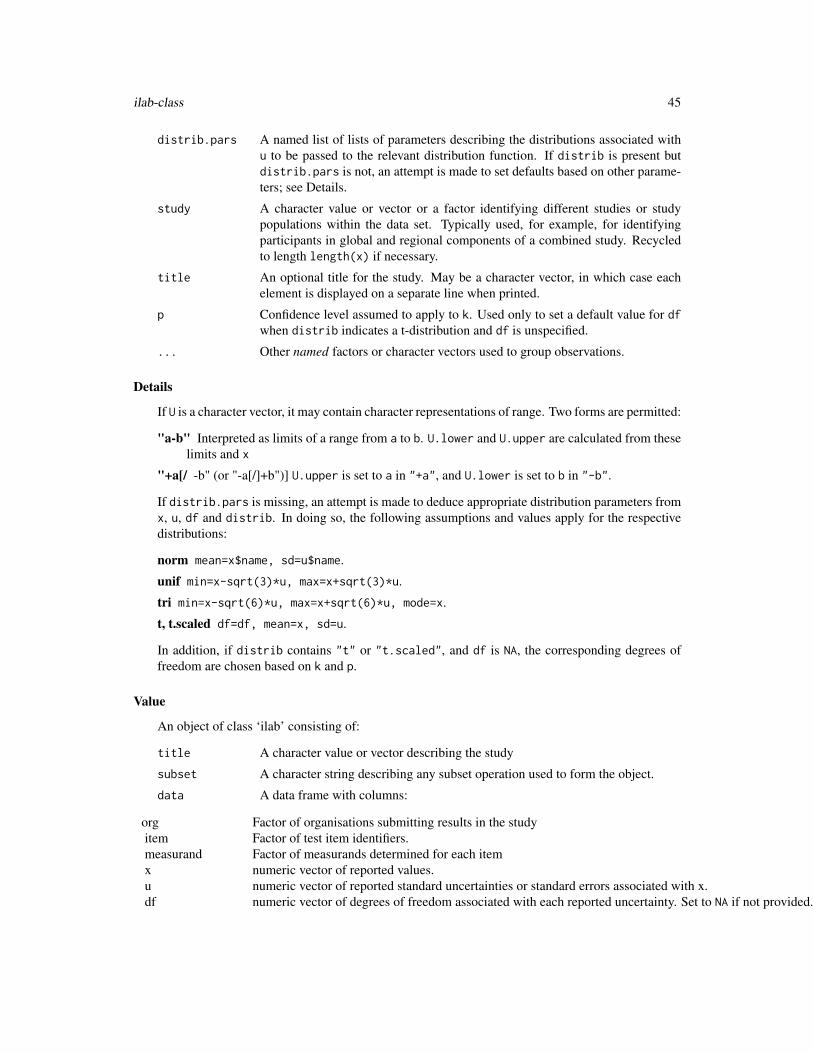
ilab-class 45

distrib.pars A named list of lists of parameters describing the distributions associated withu to be passed to the relevant distribution function. If distrib is present butdistrib.pars is not, an attempt is made to set defaults based on other parame-ters; see Details.

study A character value or vector or a factor identifying different studies or studypopulations within the data set. Typically used, for example, for identifyingparticipants in global and regional components of a combined study. Recycledto length length(x) if necessary.

title An optional title for the study. May be a character vector, in which case eachelement is displayed on a separate line when printed.

p Confidence level assumed to apply to k. Used only to set a default value for dfwhen distrib indicates a t-distribution and df is unspecified.

... Other named factors or character vectors used to group observations.

Details

If U is a character vector, it may contain character representations of range. Two forms are permitted:

"a-b" Interpreted as limits of a range from a to b. U.lower and U.upper are calculated from theselimits and x

"+a[/ -b" (or "-a[/]+b")] U.upper is set to a in "+a", and U.lower is set to b in "-b".

If distrib.pars is missing, an attempt is made to deduce appropriate distribution parameters fromx, u, df and distrib. In doing so, the following assumptions and values apply for the respectivedistributions:

norm mean=x$name, sd=u$name.

unif min=x-sqrt(3)*u, max=x+sqrt(3)*u.

tri min=x-sqrt(6)*u, max=x+sqrt(6)*u, mode=x.

t, t.scaled df=df, mean=x, sd=u.

In addition, if distrib contains "t" or "t.scaled", and df is NA, the corresponding degrees offreedom are chosen based on k and p.

Value

An object of class ‘ilab’ consisting of:

title A character value or vector describing the study

subset A character string describing any subset operation used to form the object.

data A data frame with columns:

org Factor of organisations submitting results in the studyitem Factor of test item identifiers.measurand Factor of measurands determined for each itemx numeric vector of reported values.u numeric vector of reported standard uncertainties or standard errors associated with x.df numeric vector of degrees of freedom associated with each reported uncertainty. Set to NA if not provided.

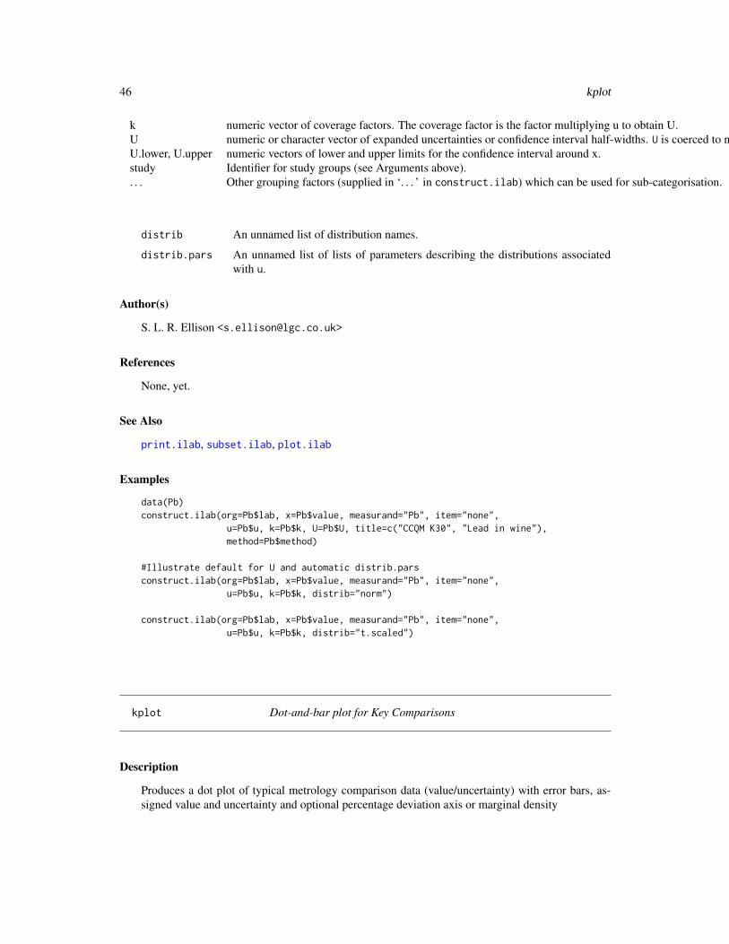
46 kplot

k numeric vector of coverage factors. The coverage factor is the factor multiplying u to obtain U.U numeric or character vector of expanded uncertainties or confidence interval half-widths. U is coerced to numeric but may include a character representation of interval limits; see Details.U.lower, U.upper numeric vectors of lower and upper limits for the confidence interval around x.study Identifier for study groups (see Arguments above).. . . Other grouping factors (supplied in ‘. . . ’ in construct.ilab) which can be used for sub-categorisation.

distrib An unnamed list of distribution names.

distrib.pars An unnamed list of lists of parameters describing the distributions associatedwith u.

Author(s)


References

None, yet.

See Also

print.ilab, subset.ilab, plot.ilab

Examples

data(Pb)construct.ilab(org=Pb$lab, x=Pb$value, measurand="Pb", item="none",

u=Pb$u, k=Pb$k, U=Pb$U, title=c("CCQM K30", "Lead in wine"),method=Pb$method)

#Illustrate default for U and automatic distrib.parsconstruct.ilab(org=Pb$lab, x=Pb$value, measurand="Pb", item="none",

u=Pb$u, k=Pb$k, distrib="norm")

construct.ilab(org=Pb$lab, x=Pb$value, measurand="Pb", item="none",u=Pb$u, k=Pb$k, distrib="t.scaled")

kplot Dot-and-bar plot for Key Comparisons

Description

Produces a dot plot of typical metrology comparison data (value/uncertainty) with error bars, as-signed value and uncertainty and optional percentage deviation axis or marginal density

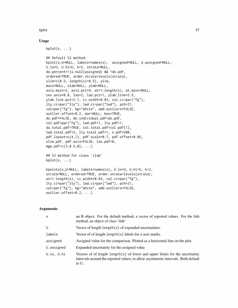
kplot 47

Usage

kplot(x, ...)

## Default S3 method:kplot(x,U=NULL, labels=names(x), assigned=NULL, U.assigned=NULL,U.lo=U, U.hi=U, k=2, strata=NULL,do.percent=!is.null(assigned) && !do.pdf,ordered=TRUE, order.strata=levels(strata),xlim=c(0.5, length(x)+0.5), ylim,main=NULL, xlab=NULL, ylab=NULL,axis.main=2, axis.pct=4, at=1:length(x), at.main=NULL,cex.axis=0.8, las=2, las.pct=1, ylab.line=2.5,ylab.line.pct=2.1, ci.width=0.03, col.ci=par("fg"),lty.ci=par("lty"), lwd.ci=par("lwd"), pch=21,col=par("fg"), bg="white", add.outliers=FALSE,outlier.offset=0.2, mar=NULL, box=TRUE,do.pdf=FALSE, do.individual.pdf=do.pdf,col.pdf=par("fg"), lwd.pdf=1, lty.pdf=1,do.total.pdf=TRUE, col.total.pdf=col.pdf[1],lwd.total.pdf=2, lty.total.pdf=1, n.pdf=200,pdf.layout=c(4,1), pdf.scale=0.7, pdf.offset=0.05,xlim.pdf, pdf.axis=FALSE, las.pdf=0,mgp.pdf=c(3,0.5,0), ...)

## S3 method for class 'ilab'kplot(x, ...)

kpoints(x,U=NULL, labels=names(x), U.lo=U, U.hi=U, k=2,strata=NULL, ordered=TRUE, order.strata=levels(strata),at=1:length(x), ci.width=0.03, col.ci=par("fg"),lty.ci=par("lty"), lwd.ci=par("lwd"), pch=21,col=par("fg"), bg="white", add.outliers=FALSE,outlier.offset=0.2, ...)

Arguments

x an R object. For the default method, a vector of reported values. For the ilabmethod, an object of class ‘ilab’

U Vector of length length(x) of expanded uncertainties

labels Vector of of length length(x) labels for x-axis marks.

assigned Assigned value for the comparison. Plotted as a horizontal line on the plot.

U.assigned Expanded uncertainty for the assigned value

U.lo, U.hi Vectors of of length length(x) of lower and upper limits for the uncertaintyintervals around the reported values, to allow asymmetric intervals. Both defaultto U.

48 kplot

k Coverage factor originally used in calculating U. Required only if do.pdf=TRUE,as k is used to calculate standard uncertainties from U. k can be a scalar (recycledto length length(x) if necessary) or a vector of length of length length(x).

strata A Factor identifying subsets of the data. Currently not implemented.

do.percent Logical indicating whether percentage deviation should be plotted as a sec-ondary axis. Defaults to TRUE if an assigned value is provided and FALSE ifthere is no assigned value or if a marginal density is required via do.pdf=TRUE.

ordered If TRUE, values are plotted in ascending order.

order.strata Character vector showing the order of plotting for strata. Currently not imple-mented.

xlim, ylim Plot limits as in plot.default.main, xlab, ylab

Titles; see ?title for details.axis.main, axis.pct

Integers specifying on which side of the plot the relevant axis is to be drawn,passed to axis as side. The axis is placed as for follows: 1=below, 2=left,3=above and 4=right. The main axis (axis.main) is provided in the same unitsas x; the percentage axis (axis.pct) shows corresponding percentage deviation.

at Vector of x-axis locations for the data points, x-axis tick marks and labels. De-faults to 1:length(x).

at.main The points at which tick-marks are to be drawn on the main (y) axis. Passed toaxis via at.

cex.axis The magnification to be used for axis annotation relative to the current settingof ’cex’. Passed to axis.

las, las.pct Integers defining x- and y axis and percentage axis label orientation; see par(las).ylab.line, ylab.line.pct

Margin lines for main and percentage axis titles. Passed to axis.

ci.width Width of error bar terminators, passed to arrows.col.ci, lty.ci, lwd.ci

Graphical parameters for the error bars; passed to arrows.

pch, col, bg Graphical parameters for data points, passed to points. bg specifies the fillcolour for pch from 21 to 25.

add.outliers If TRUE, points outside ylim are indicated as an arrow indicating the direction inwhich the omitted points lie, with a text label showing the reported value.

outlier.offset X-offset (in x-axis units) specifying lateral location of outlier tet labels relativeto x-axis location of the outlier indicator.

mar Plot margins as in par(mar). The default varies depending on do.pct anddo.pdf.

box If TRUE, a box is drawn round the plot region.

do.pdf If TRUE, a marginal density and/or individual densities for the individual reportedvalues are plotted based on the reported values x and standard uncertainties cal-culated as U/k.

kplot 49

do.individual.pdf

Logical controlling whether the individual densities are plotted as well as/insteadof the combined density.

col.pdf, lwd.pdf, lty.pdf

Graphical parameters controlling the appearance of the marginal density plot(s).Vectors are permitted, allowing different styles for each individual pdf.

do.total.pdf Logical controlling whether the sum of individual densities is plotted.col.total.pdf, lwd.total.pdf, lty.total.pdf

Graphical parameters controlling the appearance of the marginal density plot forthe combined density.

n.pdf Number of points used to construct the marginal density.

pdf.layout Vector of length 2 specifying the relative sizes of the main plot and marginaldensity plot. See ?layout for details.

pdf.scale, pdf.offset

Offset and scaling factor used to control the location and height of the marginaldensity plot(s).

xlim.pdf Controls the x-axis (i.e. the horizontal axis) for the marginal density plottingarea.

pdf.axis If TRUE and no other axis has been plotted to the right of the main plot, an axisis plotted with the marginal density.

las.pdf, mgp.pdf

Axis control parameters passed to axis to plot the axis for the marginal density.

... Parameters passed to other functions; currently unused.

Details

If do.pdf=TRUE a marginal density plot is added. This plot is constructed from a set of (currently)normal densities centred at x with standard deviation U/k.

If a marginal density is plotted, par("layout") is changed to pdf.layout; otherwise, par("layout")is set to matrix(1). Both override any previously set layout. par("layout") is preserved on exit.

The ‘ilab’ method passes all parameters in ‘. . . ’ to the default method with default values for x,upper and lower bounds U.lo and U.hi, labels and title taken from the ilab object.

kpoints is a convenience function for adding points with confidence intervals to an existing plot.kpoints is not a generic function and requires a vector x. Note that kpoints does not check for thepresence of a marginal density plot.

Value

Invisibly returns a list with components:

order The order for plotting the original data, as returned by order.

at x-axis locations used, in plotting order.

Author(s)


50 LCS

See Also

arrows.

Examples

data(Pb)kplot(Pb$value, Pb$U, assigned=2.99, U.assigned=0.06)kplot(Pb$value, Pb$U, assigned=2.99, U.assigned=0.06, do.pdf=TRUE)

#Use of return value for annotationkp<-kplot(Pb$value, Pb$U, assigned=2.99, U.assigned=0.06)text(kp$at, Pb$value-Pb$U, Pb$lab, srt=90, pos=4, cex=0.7)

LCS LCS: Largest consistent subset

Description

Calculates a ’largest consistent subset’ given values and associated uncertainty information.

Usage

LCS(x, u, p = 0.05, method = "enum", simplify = FALSE,verbose = FALSE)

Arguments

x Vector of observations.

u Vector of standard errors or standard uncertainties associated with x.

p Significance level at which consistency is tested.

method Subset identification method. Currently only ’enum’ is supported.

simplify If simplify is TRUE, only the lowest-uncertainty subset is returned even if sev-eral are of the same size.

verbose Logical: Controls the level of reporting during the search.

Details

LCS obtains the largest subset(s) of x which pass a chi-squared test for consistency, taking theuncertainties u into account.

method controls the search method used. Method "enum" uses complete enumeration of all subsetsof size n, starting at n==length(x) and decreasing n until at least one consistent subset is found.No other method is currently supported; if a different method is specified, LCS provides a warningand continues with "enum".

LCS 51

There may be more than on consistent subset of size n. If so, LCS returns all such subsets unlesssimplify is TRUE, in which case LCS prints a short warning and returns the subset with smallestestimated uncertainty as estimated for the Graybill-Deal weighted mean assuming large degrees offreedom in u.

verbose controls the level of reporting. If TRUE, LCS prints the progress of the search.

The general idea of a Largest Consistent Subset as implemented here was suggested by Cox (2006),though at least one other related method has been suggested by Heydorn (2006). It has, however,been criticised as an estimator (Toman and Possolo (2009)) ; see Warning below.

Value

If there is only one subset of maximum size, or if simplify=TRUE, a vector of indices for x repre-senting the largest consistent subset.

If there is more than one subset of maximum size and simplify=FALSE, a matrix of indices inwhich the rows contain the indices of each subset.

Warning

LCS methods are essentially equivalent to unsupervised outlier rejection. In general, this resultsin a possibly extreme low estimated variance for an arbitrarily small subset (in the limit of grossinconsistency, LCS will return subsets of size 1). The estimated uncertainty calculated for theGraybill-Deal weighted mean of the subset(s) does not generally take account of the subset selectionprocess or the dispersion of the complete data set, so is not an estimate of sampling variance.

LCS is therefore not recommended for consensus value estimation. It is however, quite useful foridentifying value/uncertainty outliers.

Author(s)

S. Ellison <[email protected]>

References

Cox, M. G. (2007) The evaluation of key comparison data: determining the largest consistent subset.Metrologia 44, 187-200 (2007)

Heydorn, K. (2006) The determination of an accepted reference value from proficiency data withstated uncertainties. Accred Qual Assur 10, 479-484 (2006)

Toman, B. and Possolo, A. (2009) Laboratory effects models for interlaboratory comparisons. Ac-cred. Qual. Assur. 14, 553-563 (2009)

See Also

None.

Examples

data(Pb)with(Pb, LCS(value, U/k))

52 loc.est-class

loc.est-class The location estimate class

Description

The location estimate class contains output from a variety of estimators used in the metRologypackage.

A print method is provided.

Usage

## S3 method for class 'loc.est'print(x, ...)

Arguments

x An object of class ‘loc.est’

... Parameters passed to other functions. Currently unused.

Details

An object of class ‘loc.est’ is a list containing

x Scalar estimate of location

u Standard uncertainty (usually equivalent to standard error) of the location estimate.

df Degrees of freedom associated with the location estimate (may be NA)

xi Numeric vector of individual values contributing to the estimate

ui Numeric vector of uncertainties initially associated with xi.

dfi Numeric vector of degrees of freedom associated with ui.

u.eff Numeric vector of ‘effective uncertainties’ in xi after any additional terms or adjustments areadded (see below).

w Numeric vector of weights associated with xi (see below).

method Character string describing the method used to obtain the estimate.

method.details An optional list of additional details provided by the particular method used.

The ‘effective uncertainties’ u.eff arise from some estimation methods (for example, Mandel-Paule). These typically involve either the estimation of an additional variance term, a scale adjust-ment to the output value uncertainty or (for example in the case of the arithmetic mean) replacementof the initial individual uncertainties with some single estimate based on the dispersion of values.These adjustments are usually equivalent to replacing the estimator used with a weighted meanusing weights 1/u2

eff .

The weight vector w is not equivalent to 1/u2eff . Rather, it gives the ratio of prior weights 1/u2

eff toposterior weights, which combine prior weights with some additional weighting. Posterior weights

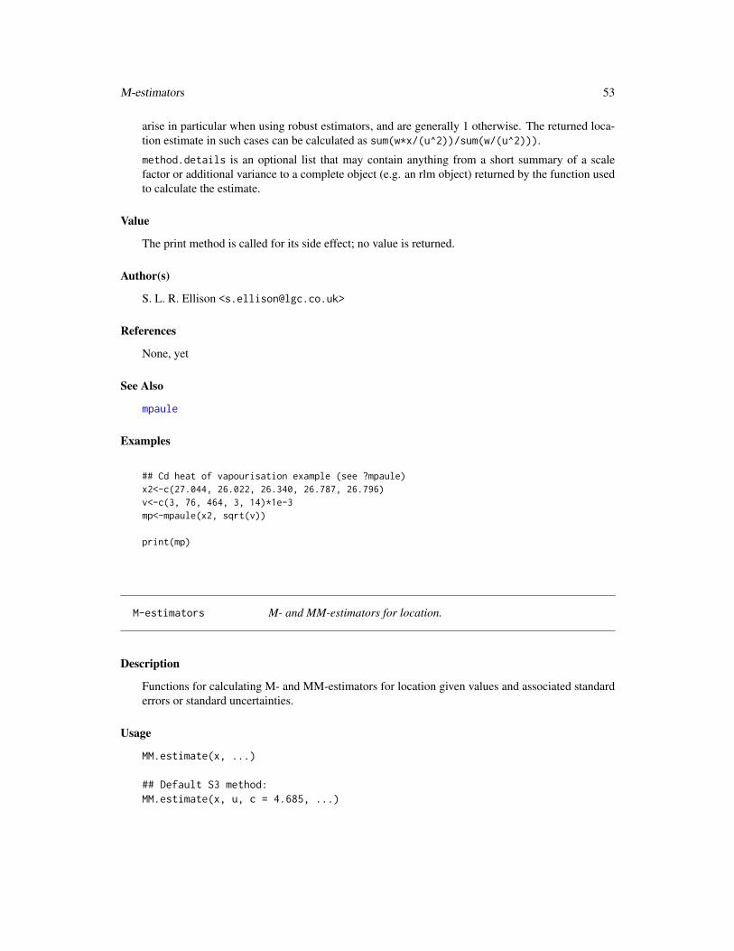
M-estimators 53

arise in particular when using robust estimators, and are generally 1 otherwise. The returned loca-tion estimate in such cases can be calculated as sum(w*x/(u^2))/sum(w/(u^2))).

method.details is an optional list that may contain anything from a short summary of a scalefactor or additional variance to a complete object (e.g. an rlm object) returned by the function usedto calculate the estimate.

Value

The print method is called for its side effect; no value is returned.

Author(s)


References

None, yet

See Also

mpaule

Examples

## Cd heat of vapourisation example (see ?mpaule)x2<-c(27.044, 26.022, 26.340, 26.787, 26.796)v<-c(3, 76, 464, 3, 14)*1e-3mp<-mpaule(x2, sqrt(v))

print(mp)

M-estimators M- and MM-estimators for location.

Description

Functions for calculating M- and MM-estimators for location given values and associated standarderrors or standard uncertainties.

Usage

MM.estimate(x, ...)

## Default S3 method:MM.estimate(x, u, c = 4.685, ...)

54 M-estimators

huber.estimate(x, ...)

## Default S3 method:huber.estimate(x, u, k= 1.345, ...)

Arguments

x numeric vector of mean values for groups

u numeric vector of standard deviations or standard uncertainties associated withthe values x

c, k Tuning parameters passed to other functions (see rlm)

... Parameters passed to other functions.

Details

These functions are wrappers for robust estimation using rlm. All simply call rlm with the formulax~1 and weights 1/u^2.

Value

An object of class ‘loc.est’.

Author(s)


References

None, yet.

See Also

rlm, loc.est-class

Examples

## Cd heat of vapourisation example## from Paule, R. C. and Mandel, J. (1982) - see ?mpaulex2<-c(27.044, 26.022, 26.340, 26.787, 26.796)v<-c(3, 76, 464, 3, 14)*1e-3

MM.estimate(x2, sqrt(v))

huber.estimate(x2, sqrt(v))

Mandel-h 55

Mandel-h Mandel’s h statistic.

Description

Density, distribution function, quantile function and random generation for Mandel’s h statistic, ameasure of relative deviation from a common mean.

Usage

dmandelh(x, g, log = FALSE)pmandelh(q, g, lower.tail = TRUE, log.p = FALSE)qmandelh(p, g, lower.tail = TRUE, log.p = FALSE)rmandelh(B, g)

Arguments

x, q vector of quantiles.

p vector of probabilities.

g number of means for which h is calculated.

B Number of observations. If ’length(B) > 1’, the length is taken to be the numberrequired.

lower.tail logical; if TRUE (default), probabilities are P[X <= x]; otherwise, P[X > x].

log, log.p logical; if TRUE, probabilities p are given as log(p).

Details

Mandel’s h is calculated for a particular mean value y[i] in a set of mean values y as h[i] = ( y[i] - mean(y) )/sd(y) )

The density, probabilities and quantiles can be derived from the beta distribution: (1+h*sqrt(g)/(g-1))/2 is distributed as Beta((g-2)/2, (g-2)/2).

Value

dmandelh returns the density at x, pmandelh the cumulative probability, qmandelh the quantiles forprobability p and rmandelh returns B random values drawn from the distribution.

Vector values of x, p, q and g are permitted, in which case the functions return vectors.

Warning

Note that rmandelh uses B and not n (as do most R random number functions) for number of randomdraws; this is for compatibility with the relevant functions for Mandel’s k, for which n is conven-tionally used for the number of replicates per group. Be careful when using named parameters!

Author(s)


56 Mandel-k

References

None.

See Also

pmandelk

Examples

#Generate the 95% and 99% quantiles for comparison with tables in#ISO 5725:1996 Part 2:n <- 3:30round(qmandelh(0.975, n), 2) #95% 2-tailed

round(qmandelh(0.995, n), 2) #99% 2-tailed

Mandel-k Mandel’s k statistic.

Description

Density, distribution function, quantile function and random generation for Mandel’s k statistic, ameasure of relative precision compared to a common variance.

Usage

dmandelk(x, g, n, log = FALSE)pmandelk(q, g, n, lower.tail = TRUE, log.p = FALSE)qmandelk(p, g, n, lower.tail = TRUE, log.p = FALSE)rmandelk(B, g, n)

Arguments

x, q vector of quantiles.

p vector of probabilities.

g number of groups for which k is calculated.

n number of observations in each group of data for which k is calculated.

B Number of observations. If ’length(B) > 1’, the length is taken to be the numberrequired.



Mandel-k 57

Details

Mandel’s k for one of a set of g standard deviations s is calculated as

k =s2ij∑p

i=1 s2ij/p

Since the numerator is chi-squared(n-1), or Gamma((n-1)/2, 2), and the denominator can be writtenas the sum of the same quantity and a pooled variance with distribution Gamma((g-1)*(n-1)/2, 2), kis distributed as Beta((n-1)/2, (g-1)(n-1)/2). Quantiles, probabilities, density and random numberscan therefore be generated from the Beta distribution. For example, qmandelk is calculated assqrt( g * qbeta( (n-1)/2, (g-1)*(n-1)/2)).

Value

dmandelh returns the density at x, pmandelh the cumulative probability, qmandelh the quantiles forprobability p and rmandelh returns B random values drawn from the distribution.

Vector values of x, p, q and g are permitted, in which case the functions return vectors.

Warning

Note that rmandelk uses B and not n (as do most R random number functions) for number of randomdraws; this is because n is conventionally used for the number of replicates per group. Be carefulwhen using named parameters!

Author(s)


References

None.

See Also

pmandelh

Examples

#Generate the 95% and 99% quantiles for comparison with tables in#ISO 5725:1996 Part 2:

round(qmandelk(0.95, g=3:30, n=3), 2) #95% upper tail

round(qmandelk(0.99, g=3:30, n=3), 2) #99% upper tail

58 Mandel-Paule

Mandel-Paule Mandel-Paule calculation

Description

Calculate a weighted mean, between-group standard deviation and standard error on the weightedmean using the Mandel-Paule algorithm.

Usage

mpaule(x, ..., tol=.Machine$double.eps^0.25, maxiter=25)

## Default S3 method:mpaule(x, u=NULL, n=NULL, groups=NULL,

tol=.Machine$double.eps^0.25, maxiter=25, ...)

mandel.paule(x, ..., tol=.Machine$double.eps^0.25, maxiter=25)

Arguments


u numeric vector of standard deviations or standard uncertainties associated withthe values x

n integer vector of numbers in each group. If NULL, u are interpreted as standarduncertainties or standard errors. n is recycled to length(x).

groups factor, or vetor which can be coerced to factor, of groups. If present, x is inter-preted as a vector of individual observations and u and n ignored.

... Additional parameters passed to other functions.

tol numeric tolerance; iteration stops when the variance step size drops below tol*var(x)

maxiter numeric maximum number of iterations

Details

The Mandel-Paule algorithm finds the between-method variance by iteratively solving the equationrelating the weighted mean to the weighting factor applied. The weighting factor is the inverse ofthe sum of the standard error in x and the between-group variance.

If the iterative procedure produces a negative estimate for the between-group variance, the between-group variance is set to zero.

For the default method, if u is present and n=NULL, u is interpreted as a vector of standard uncer-tainties or standard errors. If n is not NULL, u is interpreted as a vector of standard deviations andstandard errors are calculated as u/sqrt(n). If groups is not NULL, x is interpreted as a vectorof individual observations grouped by groups, and the algorithm is applied to the correspondinggroup means and standard errors.

mandel.h 59

If maxiter is set less than 1, no iterations are performed and the consensus mean is returned as NA.

mandel.paule is an alias for mpaule retained for backward compatibility.

Value

A loc.est object; see loc.est for details. In the returned object, df is set to n − 1 where n is thenumber of non-NA observations or group means as appropriate, and method.details is returned as:

var.between the estimated between-group variance)

iter the number of iterations taken

converged converged indicates the convergence status. 0L indicates failure to converge(maxiter reached before step size drops below tolerance); 1L indicates normalconvergence; 2L indicates that the final step size resulted in a negative between-group variance, at which point the variance and step size are set to 0.0

Author(s)

S. Cowen <[email protected]> with amendments by S. L. R. Ellison.

References

Paule, R. C. and Mandel, J. (1982), J Res Nat Bur Stand, 87, (5) 377-385

Examples

## the second example in the paper cited abovex <- c(201.533, 216.55)s <- c(0.154, 0.25)n <- c(6, 2)

mpaule(x, s/sqrt(n))

## Cd heat of vapourisation example from the paper cited abovex2<-c(27.044, 26.022, 26.340, 26.787, 26.796)v<-c(3, 76, 464, 3, 14)*1e-3mpaule(x2, sqrt(v))

mandel.h Calculate Mandel’s h statistics for replicate observations

Description

mandel.h calculates Mandel’s h statistics for replicate observations. Mandel’s h is an indication ofrelative deviation from the mean value.

60 mandel.h

Usage

mandel.h(x, g = NULL, m = NULL, na.rm = T, rowname = NULL,method=c("classical", "robust"), n = NA, ...)

## Default S3 method:mandel.h(x, g = NULL, m = NULL, na.rm = T, rowname = NULL,method=c("classical", "robust"), n = NA, ...)

## S3 method for class 'ilab'mandel.h(x, g = NULL, m = NULL, na.rm = T, rowname = NULL,method=c("classical", "robust"), n = NA, ...)

Arguments

x An R object (see Details below), which contains replicate observations or, if gis absent, means or standard deviations.

g A primary grouping factor, usually corresponding to Laboratory in an inter-laboratory study. If not present, x is taken as a set of means or standard de-viations (depending on whether type is "h" or "k".

m A secondary grouping factor, usually corresponding to test item or measuredquantity. m is ignored if x has more than one column.

na.rm A logical value indicating whether ’NA’ values should be stripped before thecomputation proceeds. Passed to functions such as mean and sd.

rowname A single character label for the primary grouping factor (e.g. "Lab", "Organisa-tion").

method Character scalar giving the calculation method. "classical" gives the tradi-tional calculation; "robust" gives a robust variant (see Details).

n scalar number of observations per group. Required only if x consists of calcu-lated standard deviations.

... Additional parameters passed to hubers when method="robust".

Details

mandel.h is a convenience wrapper for mandel.kh(..., type="h"). It is generic, with methods fornumeric vectors, arrays, data frames, matrices and objects of class 'ilab'. All parameters arepassed to mandel.kh.

Mandel’s h is an indicators of relative deviation for grouped sets of observations. Given a set ofobservations xijl where i, j, l denotes observation l, l = 1, 2, ...n for measurand or test item j andgroup (usually laboratory) i, i = 1, 2, ...p, Mandel’s h is given by:

h =x̄ij − x̄jsj

where sj =√∑p

i=1(x̄ij−x̄j)p−1

If x is a vector, one-dimensional array or single-column matrix, values are aggregated by g and, ifpresent, by m. If x is a data frame or matrix, each column is aggregated by g and m silently ignored

mandel.h 61

if present. In all cases, if g is NULL or missing, each row (or value, if a vector) in x is taken as apre-calculated mean (for Mandel’s h) or standard deviation (for Mandel’s k).

If x is an object of class 'ilab', g defaults to '$org' and m to $measurand.

The returned object includes a label ('grouped.by') for the primary grouping factor. For the'ilab' method, this is "Organisation". For other methods, If rowname is non-null, rowname isused. If rowname is NULL, the default is deparse(substitute(g)); if g is also NULL or missing,"Row" is used.

If method="robust", Mandel’s h is replaced by a robust z score calculated by replacing x̄j and sjwith the robust estimates of location and scale obtained using Huber’s estimate with tuning constantk set to 1.5 (unless otherwise specified in ...).

Value

mandel.h returns an object of class "mandel.kh", which is a data frame consisting of the requiredMandel’s statistics and in which each row corresponds to a level of g and each column to a level ofm or (if x was a matrix or data frame) to the corresponding column in x. In addition to the class, theobject has attributes:

’mandel.type’ "h" or "k"

’grouped.by’ Character scalar giving the label used for the grouping factor g; see Details abovefor the defaults.

’n’ Number of observations per group (n if specified

Author(s)


References


See Also

mandel.k, mandel.kh; pmandelh, pmandelk for probabilities, quantiles etc.; plot.mandel.kh,barplot.mandel.kh for plotting methods.

Examples

data(RMstudy)

#Data frame examples: note no secondary grouping factorh <- with(RMstudy, mandel.h(RMstudy[2:9], g=Lab))plot(h, las=2)

#Vector variantRMstk <- stack(RMstudy[,2:9])names(RMstk) <- c("x", "meas")

62 mandel.k

#names replace 'values' and 'ind'RMstk$Lab <- rep(RMstudy$Lab, 8)h2 <- with(RMstk, mandel.h(x, g=Lab, m=meas, rowname="Laboratory"))#Note use of rowname to override gplot(h2, las=2)

#ilab methodRM.ilab <- with(RMstk, construct.ilab(org=Lab, x=x, measurand=meas,item=factor(rep("CRM", nrow(RMstk))) ) )

plot(mandel.h(RM.ilab))

#Robust varianthrob <- with(RMstudy, mandel.kh(RMstudy[2:9], g=Lab, type="h", method="robust"))plot(hrob, las=2)

mandel.k Calculate Mandel’s k statistics for replicate observations

Description

mandel.k calculates Mandel’s k statistics for replicate observations. Mandel’s k an indicator ofprecision compared to the pooled standard deviation across all groups.

Usage

mandel.k(x, g = NULL, m = NULL, na.rm = T, rowname = NULL,method=c("classical", "robust"), n = NA, ...)

## Default S3 method:mandel.k(x, g = NULL, m = NULL, na.rm = T, rowname = NULL,method=c("classical", "robust"), n = NA, ...)

## S3 method for class 'ilab'mandel.k(x, g = NULL, m = NULL, na.rm = T, rowname = NULL,method=c("classical", "robust"), n = NA, ...)

Arguments




mandel.k 63





... Additional parameters passed to other methods. Currently not implemented.

Details

mandel.k is a convenience wrapper for mandel.kh(..., type="k"). It is generic, with methods fornumeric vectors, arrays, data frames, matrices and objects of class 'ilab'. All parameters arepassed to mandel.kh.

Mandel’s k is an indicator of relative dispersion for grouped sets of observations. Given a set ofobservations xijl where i, j, l denotes observation l, l = 1, 2, ...n for measurand or test item j andgroup (usually laboratory) i, i = 1, 2, ...p, Mandel’s k is given by:

k =

√s2ij∑p

i=1 s2ij/p

where sij is the standard deviation of values xijk over k = 1, 2, ..., n.

If x is a vector, one-dimensional array or single-column matrix, values are aggregated by g and, ifpresent, by m. If x is a data frame or matrix, each column is aggregated by g and m silently ignoredif present. In all cases, if g is NULL or missing, each row (or value, if a vector) in x is taken as apre-calculated mean (for Mandel’s h) or standard deviation (for Mandel’s k).



If method="robust", Mandel’s k is calculated by replacing the classical pooled standard deviationwith the robust pooled standard deviation calculated by algorithm S (see algS).

Value

mandel.k returns an object of class "mandel.kh", which is a data frame consisting of the requiredMandel’s statistics and in which each row corresponds to a level of g and each column to a level ofm or (if x was a matrix or data frame) to the corresponding column in x. In addition to the class, theobject has attributes:




64 mandel.kh

Author(s)


References


See Also

mandel.h, mandel.kh; pmandelh, pmandelk for probabilities, quantiles etc.; plot.mandel.kh,barplot.mandel.kh for plotting methods.

Examples

data(RMstudy)

#Data frame examples: note no secondary grouping factorh <- with(RMstudy, mandel.k(RMstudy[2:9], g=Lab))plot(h, las=2)

#Vector variantRMstk <- stack(RMstudy[,2:9])names(RMstk) <- c("x", "meas")#names replace 'values' and 'ind'RMstk$Lab <- rep(RMstudy$Lab, 8)h2 <- with(RMstk, mandel.k(x, g=Lab, m=meas, rowname="Laboratory"))#Note use of rowname to override gplot(h2, las=2)


plot(mandel.k(RM.ilab))

#Robust variantkrob <- with(RMstudy, mandel.kh(RMstudy[2:9], g=Lab, type="k", method="robust"))plot(krob, las=2)

mandel.kh Calculate Mandel’s h and k statistics for replicate observations

mandel.kh 65

Description

mandel.kh calculates Mandel’s h and k statistics for replicate observations. These are traditionallyused to provide a rapid graphical summary of results from an inter-laboratory exercise in which eachorganisation provides replicate observations of one or more measurands on one or more test items.Mandel’s h is an indication of relative deviation from the mean value; Mandel’s k is an indicator ofprecision compared to the pooled standard deviation across all groups.

Usage

mandel.kh(x, g = NULL, m = NULL, na.rm = T, rowname = NULL,type = c("h", "k"), method=c("classical", "robust"), n = NA, ...)

## Default S3 method:mandel.kh(x, g = NULL, m = NULL, na.rm = T, rowname = NULL,type = c("h", "k"), method=c("classical", "robust"), n = NA, ...)

## S3 method for class 'data.frame'mandel.kh(x, g = NULL, m = NULL, na.rm = T, rowname = NULL,type = c("h", "k"), method=c("classical", "robust"), n = NA, ...)

## S3 method for class 'matrix'mandel.kh(x, g = NULL, m = NULL, na.rm = T, rowname = NULL,type = c("h", "k"), method=c("classical", "robust"), n = NA, ...)

## S3 method for class 'array'mandel.kh(x, g = NULL, m = NULL, na.rm = T, rowname = NULL,type = c("h", "k"), method=c("classical", "robust"), n = NA, ...)

## S3 method for class 'ilab'mandel.kh(x, g = NULL, m = NULL, na.rm = T, rowname = NULL,type = c("h", "k"), method=c("classical", "robust"), n = NA, ...)

Arguments






type Character denoting the statistic to be calculated; may be "h" or "k".

66 mandel.kh



... Additional parameters passed to hubers when method="robust" and type="h".

Details

mandel.kh can be called directly, but is usually intended to be called via convenience functionsmandel.h or mandel.k.

mandel.kh is a generic, with methods for numeric vectors, arrays, data frames, matrices and objectsof class 'ilab'.

Mandel’s statistics are simple indicators of relative deviation or precision for grouped sets of ob-servations. Given a set of observations xijl where i, j, l denotes observation l, l = 1, 2, ...n formeasurand or test item j and group (usually laboratory) i, i = 1, 2, ...p, Mandel’s h and k are givenby:

h =x̄ij − x̄jsj

where sj =√∑p

i=1(x̄ij−x̄j)p−1

and

k =

√s2ij∑p

i=1 s2ij/p

where sij is the standard deviation of values xijk over k = 1, 2, ..., n.

If x is a vector, one-dimensional array or single-column matrix, values are aggregated by g and, ifpresent, by m. If x is a data frame or matrix, each column is aggregated by g and m silently ignoredif present. In all cases, if g is NULL or missing, each row (or value, if a vector) in x is taken as apre-calculated mean (for Mandel’s h) or standard deviation (for Mandel’s k).



If method="robust", Mandel’s h is replaced by a robust z score calculated by replacing x̄j andsj with the robust estimates of location and scale obtained using Huber’s estimate with tuningconstant k set to 1.5 (or as included in ...), and Mandel’s k is calculated by replacing the classicalpooled standard deviation in the denominator with the robust pooled standard deviation calculatedby algorithm S (see algS).

Value

mandel.kh returns an object of class "mandel.kh", which is a data frame consisting of the requiredMandel’s statistics and in which each row corresponds to a level of g and each column to a level ofm or (if x was a matrix or data frame) to the corresponding column in x. In addition to the class, theobject has attributes:

mandel.kh 67




Author(s)


References


See Also

mandel.h, mandel.k for convenience functions; pmandelh, pmandelk for probabilities, quantilesetc.; plot.mandel.kh, barplot.mandel.kh for plotting methods. algS and hubers for robustestimates used when method="robust".

Examples

data(RMstudy)

#Data frame examples: note no secondary grouping factorh <- with(RMstudy, mandel.kh(RMstudy[2:9], g=Lab, type="h"))plot(h, las=2)

k <- with(RMstudy, mandel.kh(RMstudy[2:9], g=Lab, type="k"))plot(k, las=2)

#Vector variantRMstk <- stack(RMstudy[,2:9])names(RMstk) <- c("x", "meas")#names replace 'values' and 'ind'RMstk$Lab <- rep(RMstudy$Lab, 8)h2 <- with(RMstk, mandel.kh(x, g=Lab, m=meas, rowname="Laboratory"))#Note use of rowname to override gplot(h2, las=2)


plot(mandel.kh(RM.ilab, type="h"))

#Robust variantshrob <- with(RMstudy, mandel.kh(RMstudy[2:9], g=Lab, type="h", method="robust"))plot(hrob, las=2)

68 methods.ilab

krob <- with(RMstudy, mandel.kh(RMstudy[2:9], g=Lab, type="k", method="robust"))plot(krob, las=2)

methods.ilab Methods for the ’ilab’ class.

Description

Functions for printing and plotting interlaboratory study objects objects of class ‘ilab’.

Usage

## S3 method for class 'ilab'print(x, ..., digits = NULL, right = FALSE)

## S3 method for class 'ilab'plot(x, ...)

Arguments

x An object of class ‘ilab’

digits Number of digits to display in budget and (if present) distribution parameterlists. Passed to format for distribution parameter list and to print.data.framefor output.

right If TRUE, strings in uncertainty budget are right-justified. This differs from thedefault in print.data.frame.

... Parameters passed to other functions

Details

The print method uses print.data.frame to display the data after formatting the distrib anddistrib.pars elements.

The plot method passes the object to kplot.

Value

The print and plot methods are called for their side effects.

Author(s)


References

None, yet.

mle.1wre 69

See Also

ilab-class, subset.ilab kplot.

Examples

data(Pb)il.pb<-construct.ilab(org=Pb$lab, x=Pb$value, measurand="Pb", item="none",

u=Pb$u, k=Pb$k, U=Pb$U, title=c("CCQM K30", "Lead in wine"), method=Pb$method)

print(il.pb)

plot(il.pb)

mle.1wre Vangel-Rukhin Maximum Likelihood Estimate

Description

Calculate a weighted mean, between-group standard deviation and standard error on the weightedmean using the Maximum likelihood algorithm of Vangel-Rukhin.

Usage

mle.1wre(x, s2, n, init.mu = mean(x), init.sigma2 = var(x), labels = c(1:length(x)),max.iter = 200, tol = .Machine$double.eps^0.5, trace = FALSE)

Arguments

x numeric vector of the sample mean values of each group

s2 numeric vector of the sample variances of each group

n integer vector of sample size of each group

init.mu numeric initial value for the mean

init.sigma2 numeric initial value for the between-group component of variance

labels vector of group names. Coerced to character on use.

max.iter numeric maximum number of iterations

tol numeric tolerance; iteration stops when the relative step size drops below ’tol’

trace when TRUE shows the sequence of intermediate results

70 mle.1wre

Details

The Vangel-Rukhin MLE algorithm finds the between-method variance by iteratively solving theequation relating the weighted mean to the weighting factor applied. The weighting factor is theinverse of the sum of the standard error in ’x’ and the between-method variance, scaled by thebetween-method variance.

For the default method, ’s2’ is interpreted as a vector of sample variances. ’x’ is interpreted as avector of sample means and the algorithm is applied to the corresponding group means, variances,and sample sizes.

The Vangel-Rukhin MLE algorithm shows an improvement in the number of iterations required toconverge over the classical MLE based on the Score equations.

The function mle.1wre implements the MLE for the one way random effects based on the Fisherscoring equations and is provided for comparison purpose only.

Value

mle.1wre returns an object of class "summary.mle.1wre" which contains the following fields:

mu the estimated mean

var.mu the variance associated with the estimated mean

sigma2 the estimated between variance component

llh the log likelihood of the estimates

tot.iter the total number of iterations rancur.rel.abs.error

the current relative absolute error reached

sigmai2 a vector with the estimates of the within variance components

Author(s)

H. Gasca-Aragon

References

Vangel, M. G. and Rukhin, A. L. (1999), Biometrics, Vol 55, No. 1 pp 129-136

Searle, S. R., Cassella, G., and McCulloch, C. E. (1992). Variance Components. New York: Wiley.

See Also

vr.mle, loc.est-class

Examples

##===================================================================## the dietary fiber in apples example in the Vangel and Rukhin paper##===================================================================

m1 <- c(12.46, 13.035, 12.44, 12.87, 13.42, 12.08, 13.18, 14.335, 12.23)

msd 71

s1 <- c(0.028, 0.233, 0.325, 0.071, 0.339, 0.325, 0.099, 0.064, 0.212)n1 <- c(2, 2, 2, 2, 2, 2, 2, 2, 2)

mle.1wre(m1, s1^2, n1, tol=1e-6)

# output:# 12.90585# 0.2234490# 0.4262122# 12.46790 13.34380# 6

msd Median scaled difference

Description

Generates median of scaled differences from each point in a data set to all other points..

Usage

msd(x, s=mad , ...)

Arguments

x Vector of observations

s Either a function returning an estimate of scale for x or a vector of lengthlength(x) of standard errors or standard uncertainties in x.

... Parameters passed to s if s is a function.

Details

For each observation x[i], msd calculates the median of |x[i]-x[j]|/sqrt(s[i]^2+s[j]^2), j!=i,that is, the median of differences divided by the estimated uncertainties of the distance.

If s is a function, it is applied to x and replicated to length length(x); if a scalar, it is replicated tolength length(x).

The median scaled difference is a measure of how ‘far’ an individual observation is from the major-ity of the other values in the data set. As a rule of thumb, values above 2 are indicative of a suspect(x[i], s[i]) data pair; that is, a value x[i] that is remote from a large fraction of the remainingdata given its associated standard error or standard uncertainty s[i].

72 MSD-class

Value

An object of class "MSD", consisting of a vector of length length(x) of median scaled absolutedeviations for each observation, with attributes:

names character vector of names, taken from x

x values supplied as x

s values supplied as s

Print and plotting methods are currently provided for the "MSD" class; see MSD-class.

Author(s)


See Also

pmsd, qmsd, MSD-class.

Examples

data(Pb)msd(Pb$value) # Uses mad(Pb$value) as scale estimatemsd(Pb$value, Pb$u) # Scales differences using standard uncertainties

MSD-class Methods for the object returned by msd.

Description

Print and plotting methods for the MSD object class returned by msd.

Usage

## S3 method for class 'MSD'print(x, ...)

## S3 method for class 'MSD'plot(x, type="h", ...)

## S3 method for class 'MSD'barplot(height, ylab="MSD", names.arg=names(height),crit.vals=TRUE, lty.crit=c(2,1), col.crit=2, lwd.crit=c(1,2),probs=c(0.95, 0.99), n=length(height), ... )

MSD-class 73

Arguments

x, height Object of class "MSD".

type The plot type. See plot.default.

ylab Label for vertical axis, passed to barplot

names.arg Labels for individual bars in bar plot, passed to barplot

crit.vals If TRUE, horizontal lines at critical values are added to the plot. These are calcu-lated by link{qmsd} based on supplied values of probs, n and multiple.

lty.crit, col.crit, lwd.crit

Vectors of line style parameters for plotted critical values, passed to segments.Recycled to the length of critical.values in the supplied bootMSD object.

probs vector of probabilities at which critical values are drawn.

n integer number of observations for critical value calculation; passed to qmsd.


Details

See msd for the object description.

For the barplot method, critical values are ‘single-observation’ quantiles. For use as an outlier test,use probabilities adjusted for multiple comparison; for example, for the barplot method, considerraising the default probs to the power 1/n.

Value

The print method returns the object, invisibly.

The plot method returns NULL, invisibly.

The barplot methods return the values at the midpoint of each bar.

Author(s)


See Also

msd, qmsd.

Examples

data(Pb)msd.Pb<-msd(Pb$value, Pb$u) # Uses individual standard uncertaintiesnames(msd.Pb) <- as.character(Pb$lab)

plot(msd.Pb)

barplot(msd.Pb)

74 Pb

Pb Lead in wine

Description

A data frame containing reported results for lead (in mg/kg) from CCQM Key Comparison CCQM-K30.

Usage

Pb

Format

A data frame containing 11 reported results with uncertainty data:

lab Factor giving abbreviated laboratory identifiervalue The reported value for lead (mg/kg)u Standard uncertainty (mg/kg). The values in Pb were calculated from the reported expanded

uncertainty U and coverage factor k using u=U/k.k Coverage factor. Conventionally, the coverage factor is set to a suitable quantile of Student’s t

based on the Welch-Satterthwaite effective degrees of freedom or simply set to 2 for approxi-mately 95% confidence. In this data set, labs all quoted k for approximately 95% confidence.

U Expanded uncertainty as reported by labs.method Factor indicating general measurement methodology:

IDMS Isotope dilution mass spectrometryICP Inductively coupled plasma spectrometryGFAAS Graphite furnace atomic absorbtion spectrometry

include logical; Whether the reported result was included in the calculation of the Key ComparisonReference Value for the study.

Details

The study involved circulation of a homogeneous set of samples of wine for analysis for lead (Pb)content by a number of National Measurement Institutes.

The Key Comparison Reference Value, or assigned value for the lead content, was set at 2.99 mg/kgwith expanded uncertainty 0.06 mg/kg.

Source

Hearn, R., Santamaria-Fernandez, R. and Sargent, M. (2008) Final report on key comparisonCCQM-K30: Determination of lead in wine. Metrologia 45, 08001, 2008

References

See source.

plot.d.ellipse 75

plot.d.ellipse Plot data ellipses

Description

Plots a number of data ellipses specified by

Usage

## S3 method for class 'd.ellipse'plot(x, col.ellipse = 1, lty.ellipse = 1, lwd.ellipse = 1,fill = NA, density = NULL, angle = 45, add = FALSE, npoints = 100,xlim = NA, ylim = NA,prinax = FALSE, col.prinax = 1, lty.prinax = 1, lwd.prinax = 1,xlab=NULL, ylab=NULL, ...)

Arguments

x An object of class d.ellipsecol.ellipse, lty.ellipse, lwd.ellipse

Colour, line type and line width for the ellipse(s). Can be vectors, allowingdifferent colour, line type etc. Recycled as necessary to length length(x).

fill, density, angle

Fill colour, line density and line angle for each ellipse in x. See polygon fordetails. Can be vectors. Recycled as necessary to length length(x).

add If TRUE, ellipses are added to an existing plot. If FALSE a new plot is created.

npoints Controls the number of points used to form each ellipse. See data.ellipse fordetails.

xlim, ylim Plot limits. Ignored if add == FALSE

prinax If TRUE (the default), the principal axes are drawn on the plot.col.prinax, lty.prinax, lwd.prinax

Colour, line type and line width for principal axes.

xlab, ylab Axis labels passed to plot if add == FALSE. Defaults to dimension names in xor, if those are NULL, to "X" and "Y".

... Additional arguments, passed to plot if add == TRUE.

Details

A series of ellipses specified in x is plotted. The function is primarily used for adding ellipses to aYouden plot.

Value

The function is called for its side effect, which is the drawing of ellipses.

76 plot.mandel.kh

Author(s)

S L R Ellison

See Also

data.ellipse, youden.plot

Examples

data(chromium)cov.Cr <- cov.dellipse(chromium)dellipse.Cr <- data.ellipse(cov.Cr, plot=FALSE)plot(dellipse.Cr)

plot.mandel.kh Classical plots of Mandel’s statistics.

Description

plot.mandel.kh produces classic plots of Mandel’s statistics, suitably grouped and with appropri-ate indicator lines for unusual values.

Usage

## S3 method for class 'mandel.kh'plot(x, probs = c(0.95, 0.99), main, xlab = attr(x, "grouped.by"),ylab = attr(x, "mandel.type"), ylim = NULL, las = 1,axes = TRUE, cex.axis = 1, frame.plot = axes,lwd = 1, lty = 1, col = par("col"),col.ind = 1, lty.ind = c(2, 1), lwd.ind = 1,separators = TRUE, col.sep = "lightgrey", lwd.sep = 1, lty.sep = 1,zero.line = TRUE, lwd.zero = 1, col.zero = 1, lty.zero = 1,p.adjust = "none", ...)

Arguments

x An object of class 'mandel.kh'




plot.mandel.kh 77


ylim the y limits of the plot. For Mandel’s k, the default lower limit is zero.

las the style of the axis labels; see par for details.

axes a logical value indicating whether axes should be drawn on the plot.

cex.axis The magnification to be used for axis annotation relative to the current settingof ’cex’.


lwd, lty, col Graphical parameters used for the plotted vertical lines corresponding to eachvalue of Mandel’s statistics (the plot is of type "h"). All are recycled acrossthe prinmary grouping factor, allowing different measurands/test items to beidentified more clearly.



separators Logical; if TRUE, separator lines are drawn between groups of values.col.sep, lwd.sep, lty.sep

Graphical parameters used for the separator lines.

zero.line logical; if TRUE a horizontal line is drawn at zero.lwd.zero, col.zero, lty.zero



... Other (usually graphical) parameters passed to plot.

Details

Mandel’s statistics are traditionally plotted for inter-laboratory study data, grouped by laboratory,to give a rapid graphical view of laboratory bias and relative precision. The traditional plot is a plotof type "h", that is, simple vertical lines from the x-axis.

For classical Mandel statistics, indicator lines are drawn based on qmandelh or qmandelk as appro-priate. For robust variants, indicator lines use qnorm for the h statistic and qf(probs, n, Inf) forthe k statistic. Note that this corresponds to taking the robust estimates of location and scale as truevalues, so will be somewhat anticonservative.

plot.mandel.kh uses gplot for the main plot.

Value

plot.mandel.kh returns a numeric vector of mid-points of the groups along the x-axis.

Author(s)


78 plot.uncert

References


See Also

mandel.h, mandel.k, mandel.kh, pmandelh, pmandelk for probabilities, quantiles etc.

See barplot.mandel.kh for an alternative plotting method. gplot for the underlying plottingfunction.

Examples

data(RMstudy)

h <- with(RMstudy, mandel.h(RMstudy[2:9], g=Lab))plot(h, las=2) # Lab 4 shows consistent low bias;

# Lab 23 several extreme values.

#Use colours to identify particular measurands:plot(h, las=2, col=1:8)legend("bottomleft", legend=names(h), col=1:8, lty=1, cex=0.7, bg="white")

#Example of Mandel's k:k <- with(RMstudy, mandel.k(RMstudy[2:9], g=Lab))plot(k, las=2) # Lab 8 looks unusually variable;

# Lab 14 unusually precise

plot.uncert Plot method for ’uncert’ objects

Description

Plots for uncertainty budgets produced by uncert calls.

Usage

## S3 method for class 'uncert'plot(x, which = c(1,2,4,5), main = paste(deparse(substitute(x))),

ask = prod(par("mfcol")) < length(which) && dev.interactive(),caption = list("Variance and covariance contributions",expression(sqrt(group("|", "Variance and covariance contributions", "|"))),expression("Contribution " * u[i](y) == c[i] * u[i]),"Combined contribution", "Correlation (x,y)","Covariances (x,y)"), cex.caption = 1, ...)

plot.uncert 79

Arguments

x An object of class uncert produced by a call to uncert().

which Integer in 1:6; the particular variant(s) of plot required. A vector is permitted, inwhich case plots are produced in ascending order.

main Main title for the plot

ask logical; if ’TRUE’, the user is _ask_ed before each plot, see ’par("ask=")’

caption A list of captions for all the different plots.

cex.caption Text size for captions. Note that if the number of figures per page is over 2,captions are further scaled by 0.8

... Further parameters passed to plot() (mostly barplot).

Details

For uncert objects created with methods other than MC, the plot types are:

which=1 A barplot of all non-zero contributions to the combined uncertainty. These are derivedfrom the covariance matrix and the coefficients ci. For terms on the diagonal of the covariancematrix, these are (ci ∗ ui)2; for off-diagonal terms (the correlation terms), 2 ∗ (ci ∗ ui) ∗ (cj ∗uj) ∗ rij. The threshold for deciding an off-diagonal term is nonzero is that its magnitude isgreater than 2*.Machine$double.eps. Note that off-diagonal contributions may be negative.

which=2 As for which=1 except that the square root of the absolute value is plotted. For the ’diag-onal’ terms, these are just eqnu_i(y) in the nomenclature used by the GUM.

which=3 A barplot of ui(y)2, without the correlation terms.

which=4 A barplot of the sum of all (co)variance contributions associated with each xi, that is,

contrib(i) = (ciui)2 +

∑j 6=i

2(ciui)(cjuj)ri,j

.

which=5 A barplot of the theoretical correlations cov(xi, y)/u(xi)uy .

which=6 A barplot of the theoretical covariances cov(xi, y).

Values of which outside this range are silently ignored.

For the X-Y correlation and covariance plots, the covariances are calculated from the covariancematrix V (supplied to uncert() as cov or calculated as outer(u,u,"*")*cor) and sensitivity coef-ficients ci as cov(xi, y) =

∑j Vj,icj . In fact the calculation used is simpler: cov.xy <- V %*% ci.

The correlations are calculated in turn from these using cov(xi, y)/u(xi)uy .

Perhaps the most informative plots are for which=1, which=2, which=4 and which=5. The firstof these includes all nonzero signed contributions, making the negative contributions visible; thesecond (which=2) makes direct comparison of magnitudes easier. The combined contribution plotis the effect on the total variance of removing all terms associated with a particular variable; it showshow much u2

y would reduce if the uncertainty for xi were reduced to zero. Note that in some caseswith negative correlation the combined uncertainty can increase, on dropping a variable, shownby a negative reduction in the plot. (which=5) is among the most direct indications of the relativeimportance of individual parameters.

Objects created with the MC method are passed to plot.uncertMC.

80 plot.uncertMC

Value

Invisibly returns the default return value for the last plot produced.

Author(s)


References

None.

See Also

uncert, barplot, plot.uncertMC.

Examples

#An example with negative correlationx <- list(a=1, b=3, c=2, d=11)u <- lapply(x, function(x) x/10)u.cor<-diag(1,4)u.cor[3,4]<-u.cor[4,3]<- -0.5u.form.c<-uncert(~a+b*2+c*3+d/2, x, u, method="NUM", cor=u.cor)

par(mfrow=c(3,2))plot(u.form.c, which=1:6, las=1, horiz=TRUE) #Note use of barplot parameters

plot.uncertMC Plot method for ’uncertMC’ objects

Description

Plots for uncertainty evaluations produced by uncertMC or calls to uncert with method=MC.

Usage

## S3 method for class 'uncertMC'plot(x, which = 1:2,

main=paste("Monte Carlo evaluation -",deparse(substitute(x))),ask = prod(par("mfcol")) < length(which) && dev.interactive(),caption = list("Histogram", "Q-Q plot", "Density","Correlation x-y", "Covariance x-y"),xlab = paste(deparse(substitute(x)), "$y", sep = ""),..., cex.caption = 1, cex.main = 1.25, lwd.y = 2, col.y = 2, lty.y,col.qqline = NULL, lty.qqline = NULL, lwd.qqline = NULL)

plot.uncertMC 81

Arguments

x An object of class uncertMC produced by uncertMC() or uncert() with method="MC".

which Integer in 1:5; the particular variant(s) of plot required. A vector is permitted, inwhich case plots are produced in ascending order of which.

main Main title for the plot

ask logical; if ’TRUE’, the user is _ask_ed before each plot, see ’par("ask=")’

caption A list of captions for all the different plots.

xlab x-axis label, currently passed only to the histogram plot.

... Additional parameters passed to other functions. See details for which parame-ters are passed.

cex.caption Expansion factor for individual plot captions; as cex in par.

cex.main Expansion factor for main title; as cex.main in par.lwd.y, col.y, lty.y

Line width and colour for the location line in the histogram and density plots.Setting lwd.y=0 suppresses the location line.

col.qqline, lty.qqline, lwd.qqline

Graphical parameters for the Q-Q line in the Q-Q plot.

Details

For uncert objects created with methods other than MC, the plot types are:

which=1 A histogram of the MC replicates in x$MC$y, with optional line for x$MC$y. The histogramis produced using hist.default

which=2 A Q-Q plot of the MC replicates in x$MC$y, with Q-Q line. The plot uses qqnorm.default.If datax is not present (in sQuote. . . ), it is set to TRUE.

which=3 A density plot of the MC replicates in x$MC$y. The plot calls density.default to cal-culate the density and plot.density to produce the plot.

which=4 A bar plot of eqncor(x_i,y) if x$y is present. Any correlation method supported bystats::cor may be included in ‘. . . ’ (e.g as method="pearson".

which=5 A bar plot of eqncov(x_i,y) if x$y is present. Any correlation method supported bystats::cov may be included in ‘. . . ’ (e.g as method="pearson".

Values outside 1:5 are silently ignored.

Parameters in ‘. . . ’ are passed to the various plot methods or calculations called. Only those param-eters relevant to a given plot are passed to each calculation or plotting function, so ‘. . . ’ can includeany parameter accepted by any of the functions called.

For the x-y correlation and x-y covariance plot, values in x$cor.xy are used if available. If not,stats::cor or stats::cov is called on values in x$MC$y and x$MC$x if the latter is available (i.e.uncertMC was called with keep.x=TRUE). If neither x$cor.xy nor x$MC$x is present, or if methodis unknown, the plot is skipped with a warning.

Value

plot.uncertMC invisibly returns NULL.

82 pmsd

Author(s)


References

None.

See Also

uncertMC-class, hist, qqnorm, qqline, density, plot.density

Examples

expr <- expression(a/(b-c))x <- list(a=1, b=3, c=2)u <- lapply(x, function(x) x/20)set.seed(403)u.invexpr<-uncertMC(expr, x, u, distrib=rep("norm", 3), B=999, keep.x=TRUE )par(mfrow=c(2,2))plot(u.invexpr, which=1:4, pch=20, method="k")

# method="k" gives Kendall correlation

pmsd Median scaled difference probabilities and quantiles

Description

Cumulative lower tail probability and quantile for median of scaled differences.

Usage

pmsd(q, n, sd=1, scale=TRUE)qmsd(p, n, sd=1, scale=TRUE)

Arguments

q Vector of quantiles.

p Vector of probabilities.

n Number of observations from which msd was calculated.

sd Standard deviation, used to scale q.

scale If scale is TRUE, sd is divided by sqrt(2) prior to calculating p or q.

potassium 83

Details

pmsd and qmsd implement exact (for even n) or approximate (odd n) probabilities and quantiles forthe median scaled difference applied to a single observation in a normal distribution.

n is the number of observations in the data set of interest and not the degrees of freedom or numberof differences (msd for a value x[i] in a set of n observations involves n-1 scaled differences).

The probabilities are calculated using quadrature integration over a distribution of an order statistic,and may be quite slow (seconds for a vector of several hundred 100 values of q on an Intel x86machine running at 1GHz). qmsd is obtained even more slowly by root-finding from pmsd usinguniroot.

n, p and q are recycled to the length of the longest, as necessary.

Note that both functions are appropriate for the distribution of single values. If seeking an outliertest, adjust p for n comparisons before applying qmsd.

Value

A vector of length length(p) or length(q) (or, if longer, length(n)) of quantiles or probabilitiesrespectively.

Author(s)


See Also

msd for calculation of MSD values, and bootMSD for a parametric bootstrap (MCS) method ofobtaining p-values and quantiles for the more general non-IID case.

Examples

data(Pb)msd(Pb$value) # Uses mad(Pb$value) as scale estimatemsd(Pb$value, Pb$u) # Scales differences using standard uncertainties

potassium Potassium data for two different materials included in an interlabora-tory study

Description

Potassium data for two different materials included in an interlaboratory study intended to providedata for certification of a reference material.

Usage

data("potassium")

84 rbind.ilab

Format


QC Potassium concentrations (mg/kg) reported on a material used as a quality control material

RM Potassium concentrations (mg/kg) reported on a candidate reference material material used as aquality control material

Details

Potassium data for two different materials included in an interlaboratory study intended to providedata for certification of a crab tissue reference material. The study included a previously certifiedreference material (near end of stock) to serve as a quality control (QC) check. Laboratories wereasked to report five replicate measurements on the candidate reference material and three for theQC material. Each row in the data set corresponds to the mean of replicate results reported by eachlaboratory.

Inspection of the data suggests that one laboratory interchanged or mislabelled the test materials.The anomalous results appear as an outlier for both QC and RM, as well as being visible as anoff-diagonal outlier in a Youden plot - see youden.plot).

Source

Private communication - Pending publication

Examples

data(potassium)yplot(potassium)

rbind.ilab Combine ’ilab’ objects

Description

Functions to combine ilab objects.

Usage

rbind(..., deparse.level = 1)## Default S3 method:rbind(..., deparse.level = 1)## S3 method for class 'ilab'rbind(..., deparse.level = 1)

## S3 method for class 'ilab'c(..., recursive=FALSE)

cbind(..., deparse.level = 1)

rbind.ilab 85

## Default S3 method:cbind(..., deparse.level = 1)## S3 method for class 'ilab'cbind(..., deparse.level = 1)

Arguments

... For rbind and c, objects of class ‘ilab’ to be combined.For cbind, one ’ilab’object and vectors, scalars or data frames to be appended to the ’ilab’ object’s$data element. See Details.

deparse.level integer controlling the construction of labels. Passed to rbind.data.frame orbase::cbind.

recursive logical, controlling recursion in lists. Included solely for consistency with base::c;no effect in c.ilab.

ilab object of class ‘ilab’.

Details

The generic and default cbind and rbind functions defined by metRology use the first object in'...' to decide which method to apply. This differs from the behaviour of these functions in thebase package, which dispatch based on inspection of all objects in '...' (see rbind in the basepackage for details). Control is, however, passed to the base package functions if an ilab object isnot first in the list.

The rbind method for class ’ilab’ combines objects by applying rbind to the $data elements inturn and then concatenating the $distrib and $distrib.pars elements using the default c method.

Combination of the $data elements follows the rules of rbind.data.frame; in particular, namesmust match, but need not be in the same order and the return value column classes will be coercedto match the first if necessary.

c.ilab simply passes the objects to rbind.ilab, using the default value for deparse.level.recursive is ignored. An error is returned if any objects in '...' are not of class ‘ilab’.

The cbind method for ‘ilab’ objects combines objects of class ‘ilab’ with atomic objects or dataframes by applying base::cbind to $data in the (single) supplied ilab object and the items listed in'...'. base::cbind will extend scalars, vectors or columns in data frames to length nrow(ilab$data)if their length is an integer fraction of nrow(ilab$data). Unlike base::cbind, cbind.ilab doesnot permit vectors or data frames longer than nrow(ilab$data) and will return an error in suchcases. cbind.ilab will also return an error if any objects in '...' are not one of atomic, data frameor class ‘ilab’, if more than one ‘ilab’ object is supplied or if none are.

Value

An object of class ‘ilab’. The title for the returned object is the title for the first ilab object in thelist.

For the cbind method, the returned object will have additional columns in the $data element, andthe title will be unchanged.

86 REML location estimate

Warning

Because of the unusual method dispatch behaviour of base::cbind and base::rbind, which usethe data frame method if any objects in '...' are data frames, metRology masks the base packagefunctions in order to guarantee correct dispatch when data frames are included in '...'. No adverseeffects are currently known, but please report any to the package maintainer. Calling base::cbinddirectly will provide a work-around if necessary.

Author(s)


References

None, yet.

See Also

base package functions cbind, c.

Examples

data(Pb)il1<-construct.ilab(org=Pb$lab, x=Pb$value, measurand="Pb", item="none",

u=Pb$u, k=Pb$k, U=Pb$U, title=c("CCQM K30", "Lead in wine"),method=Pb$method)

rbind(il1, il1)

REML location estimate

Restricted maximum likelihood estimate of location

Description

Calculates REML estimate of location, with standard error, assuming a random-effects model

Usage

reml.loc(x, ..., na.rm = FALSE)

## Default S3 method:reml.loc(x, s, n = NULL, groups = NULL, na.rm = FALSE,

tol=.Machine$double.eps^0.5, REML=TRUE, ...)

REML location estimate 87

Arguments


s numeric vector of length length(x) of standard deviations or standard uncer-tainties associated with the values x.

n integer giving the number of observations in each group. May be a vector oflength length(x). If n is NULL, s is interpreted as a vector of standard uncer-tainties or standard errors. n is recycled to length(x)

groups factor, or vetor which can be coerced to factor, of groups. If present, x is in-terpreted as a vector of individual observations and s and n ignored, if present,with a warning.

na.rm logical: if TRUE, NA values are removed before processing.

tol numeric tolerance for convergence, used by optimize().

REML logical: if TRUE (the default), the function optimises the REML criterion (seeDetails). If FALSE, the maximum likelihood criterion is used.

... Further parameters passed to optimize().

Details

reml.loc finds an excess variance τ2 and location µ that maximise the restricted maximum likeli-hood criterion.

The estimator assumes a model of the form

xi = µ+ bi + ei

in which bi is drawn from N(0, τ2) and ei is drawn from N(0, σ2i ).

By default the function maximises the data-dependent part of the negative log restricted likelihood:

1

2

(k∑i=1

(xi −mu)2

u2i

+

k∑i=1

log(u2i ) + log

(k∑i=1

(1/u2i )

))

where ui = s2i + τ2 and k is the number of mean values. If REML=FALSE, the final term is omitted

to give the maximum likelihood criterion.

This implementation permits input in the form of:

• means x and standard errors s, in which case neither n nor groups are supplied;

• means x, standard deviations s and group size(s) n, standard errors then being calculated ass/sqrt(n)

• individual observations x with a groupinf factor groups, in which case standard errors arecalculated from the groups using tapply.

88 RMstudy

Value

A loc.est object; see loc.est for details. In the returned object, individual values xi are alwaysinput means (calculated from groups and n as necessary); method.details is returned as a listcontaining:

mu The estimated location.

s The standard error in the location.

tau The excess variance (as a standard deviation).

REML Logical, giving the value of REML used.

Author(s)


References

None, but see documentation for the metafor package for a more general implementation of REML.

See Also

loc.est-class

Examples

#PCB measurements in a sediment from Key Comparison CCQM-K25#s are reported standard uncertaintiespcb105 <- data.frame(x=c(10.21, 10.9, 10.94, 10.58, 10.81, 9.62, 10.8),

s=c(0.381, 0.250, 0.130, 0.410, 0.445, 0.196, 0.093))

with( pcb105, reml.loc(x, s) )

RMstudy Collaborative study results for metals in a reference material certifi-cation study

Description

A data frame containing reported replicate results, in mg/L, for elements reported in an inter-laboratory certification study for a candiate drinking reference material.

Usage

data(RMstudy)

Scaled t distribution 89

Format


Lab a factor with levels Lab1 - Lab29

Arsenic a numeric vector

Cadmium a numeric vector

Chromium a numeric vector

Copper a numeric vector

Lead a numeric vector

Manganese a numeric vector

Nickel a numeric vector

Zinc a numeric vector

Details

The data set includes results for eight of a total of 23 elements studied in an inter-laboratory studyof a candidate reference material. All observations are reported in mg/l. Laboratories were askedto report 5 replicate observations for each element. Replicate observations appear on separate rows.Most but not all laboratories reported five replicates, and some laboratories reported no results forsome elements. The eight elements included in the data set are those for which no more than threelaboratories failed to report any results. Missing observations are coded NA.

Laboratories were coded anonymously in order of receipt of results.

Source

LGC limited, Teddington, UK (Private communication).

Scaled t distribution Scaled and shifted t distribution.

Description

Student’s t distribution for ’df’ degrees of freedom, shifted by ’mean’ and scaled by ’sd’.

Usage

dt.scaled(x, df, mean = 0, sd = 1, ncp, log = FALSE)pt.scaled(q, df, mean = 0, sd = 1, ncp, lower.tail = TRUE, log.p = FALSE)qt.scaled(p, df, mean = 0, sd = 1, ncp, lower.tail = TRUE, log.p = FALSE)rt.scaled(n, df, mean = 0, sd = 1, ncp)

90 Scaled t distribution

Arguments

x,q vector of quantiles.p vector of probabilities.n number of observations. If length(n) > 1, the length is taken to be the number

required.df degrees of freedom (> 0, maybe non-integer). df = Inf is allowed.mean mean value for the shifted, scaled distribution.sd Scale factor for the shifted, scaled distribution.ncp non-centrality parameter delta; currently except for rt(), only for abs(ncp) <= 37.62.

If omitted, use the central t distribution.lower.tail logical; if TRUE (default), probabilities are P[X <= x]; otherwise, P[X > x].log, log.p logical; if TRUE, probabilities p are given as log(p).

Details

These are wrappers for the corresponding t distribution functions in package stats.

The scaled, shifted t distribution has mean mean and variance sd^2 * df/(df-2)

The scaled, shifted t distribution is used for Monte Carlo evaluation when a value x has been as-signed a standard uncertainty u associated with with df degrees of freedom; the correspondingdistribution function for that is then t.scaled with mean=x, sd=u and df=df.

Value

dt.scaled gives the density, pt.scaled gives the distribution function, qt.scaled gives the quan-tile function, and rt.scaled generates random deviates.

Invalid arguments will result in return value NaN, with a warning.

Author(s)


See Also

TDist

Examples

u<-rt.scaled(20, df=5, mean=11, sd=0.7)

qt.scaled(c(0.025,0.975), Inf, mean=10, sd=1) #10 +- 1.96*sd

require(graphics)hist(rt.scaled(10000, df=4, mean=11, sd=0.7), breaks=50, probability=TRUE)x<-seq(0,25, 0.05)lines(x,dnorm(x,mean=11, sd=0.7), col=2)

Triangular 91

Triangular The triangular distribution.

Description

Density, distribution function, quantile function and random generation for the triangular distribu-tion with range ’min’ to ’max’ and mode equal to ’mode’.

Usage

dtri(x, min=-sqrt(6), max=sqrt(6), mode = (min + max)/2,log = FALSE)

ptri(q, min=-sqrt(6), max=sqrt(6), mode = (min + max)/2,lower.tail = TRUE, log.p = FALSE)

qtri(p, min=-sqrt(6), max=sqrt(6), mode = (min + max)/2,lower.tail = TRUE, log.p = FALSE)

rtri(n, min=-sqrt(6), max=sqrt(6), mode = (min + max)/2)

Arguments

x, q Vector of quantiles.

p Vector of quantiles.

n Number of observations. If ’length(n) > 1’, the length is taken to be the numberrequired.

min Vector of lower limits of distribution.

max Vector of upper limits of distribution.

mode Vector of modes



Details

The triangular distribution has density

f(x) = 2 ∗ (x−min)/((max−min) ∗ (mode−min))(min < x <= mode)

f(x) = 2 ∗ (max− x)/((max−min) ∗ (max−mode))(mode < x < max)

and 0 elsewhere.

The mean is1

3(min+mode+max)

92 uncert

and the variance is

1

18(min2 +mode2 +max2 −min ∗mode−min ∗max−mode ∗max)

The default values of min, max and mode give a distribution with mean 0 and unit variance.

If min>max, min amd max will be silently interchanged. If mode is not within [min, max], thefunctions return NA, with a warning.

rtri calls runif(n, 0, 1) to generate probabilities which are passed to qtri.

Value

A vector of densities, probabilities, quantiles or random deviates. dtri gives the density, ptri givesthe distribution function, qtri gives the quantile function, and rtri generates random deviates.

Author(s)


See Also

runif

Examples

require(graphics)x<-seq(-3,3,0.02)

par(mfrow=c(2,1))plot(x, dtri(x), type="l", main="Density")plot(x, ptri(x), type="l", main="p(X<x)")

u <- rtri(5000)

var(rtri(10000,-1,1)) # ~ = 1/6 = 0.167

uncert Uncertainty estimation functions

Description

Functions for estimating measurement uncertainty from standard uncertainties and either sensitivitycoefficients or (for some methods) expressions or functions. Correlation is supported via either acorrelation or covariance matrix.

uncert 93

Usage

uncert(obj, ...)

## Default S3 method:uncert(obj, c, method = c("GUM", "MC"), cor,

cov, distrib=NULL, distrib.pars=NULL, B=200, x=NULL, keep.x = TRUE,u=obj, ...)

## S3 method for class 'expression'uncert(obj, x, u, method=c("GUM", "NUM", "kragten", "k2", "MC"),

cor, cov, distrib=NULL, distrib.pars=NULL,B=200, delta=0.01, keep.x = TRUE, ...)

## S3 method for class 'function'uncert(obj, x, u, method=c("NUM", "kragten", "k2", "MC"),


## S3 method for class 'formula'uncert(obj, x, u, method=c("GUM", "NUM", "kragten", "k2", "MC"),


Arguments

obj An R object used for method dispatch; see below. Methods currently exist fornumeric vector, expression, function, or formula

u For the default method, a numeric vector of standard uncertainties. For theformula or expression methods, a named list of standard uncertainties.Note thatfor the default method, u is set to the value of obj, allowing specification ofeither as the first argument

c A numeric vector of senstivity coefficients.

x For the expression or formula methods, an R object which can be used as anenvironment by eval. For the function method, a list of parameters supplied toFUN via do.call.

method Method of uncertainty evaluation. The current list of methods is:

GUM First-order error propagation (the “law of propagation of uncertainty”)as implemented by the GUM.

NUM Numerical differentiation using a simple small step size.kragten Numerical estimation of uncertainty following Kragten (Kragten (1994).k2 A symmetric modification of Kragten’s approach described by Ellison (El-

lison (2005)).MC Monte Carlo simulation.

cor, cov A (square, symmetric) correlation or covariance matrix, respectively. If neitheris specified, cor is set to the identity matrix.

94 uncert

distrib For method="MC", a character vector of length length(x) or a named list ofnames of distribution functions associated with u. See Details for defaults. Thelist format may include user-specified functions. Silently ignored for other meth-ods.

distrib.pars For method="MC", a list of lists of parameters describing the distributions asso-ciated with u to be passed to the relevant distribution function. If distrib ispresent but distrib.pars is not, neither are included in the return value unlessmethod="MC". See Details for defaults when method="MC". Silently ignored forother methods.

B Number of Monte Carlo replicates.

delta Step size for numerical differentiation.

keep.x For method="MC", if keepx=TRUE, the simulated replicates of x are included inthe return object.

... Additional parameters to be passed to a function (for the function method) orused in an expression (for expression or formula method).

Details

The default “GUM” method applies first-order error propagation principles to estimate a combinedstandard uncertainty from a set of sensitivity coefficients and either a set of standard uncertaintiesand a correlation matrix (which defaults to an identity matrix) or a covariance matrix. Both optionsuse the same calculation, which is simply (t(c) %*% cov) %*% c ; standard uncertainties are firstcombined with the correlation matrix provided to form the covariance matrix. Since the correlationmatrix defaults to the identity matrix, the default is combination without correlation.

The default method takes obj as a vector of uncertainty contributions unless u is specified, in whichcase u is used. It is not necessary to specify both. The expression method requires obj to bea differentiable R expression which can be evaluated in the environment x to provide a numericvalue. For the function method, obj must be an R function which takes parameters from x andreturns a numeric value. For the formula method, obj must be a formula with no left-hand side (e.g.~a*x+b*x^2) which can be evaluated in the environment x to provide a numeric value.

The formula and expression methods first calculate derivatives for the expression or formula, eval-uate them using the supplied values of x and then pass the resulting sensitivity coefficients, withsupplied u, cor or cov to uncert.default.

The derivatives for the “GUM” method (formula and expression methods only) are algorithmicderivatives (that is, algebraic or analytical derivatives) obtained using deriv applied to expr andformula.

Numerical derivatives are computed in different ways depending on the method specified:

- For method="NUM", the derivatives are calculated as (f(x+ delta ∗ u)− f(x− delta ∗ u))/(2 ∗delta ∗ u).

- For method="kragten", derivatives are calculated as (f(x+ u ∗ sign(delta))− f(x))/u.

- For method="k2", derivatives are calculated as (f(x+ u)− f(x− u))/(2 ∗ u).

"NUM" is likely to give a close approximation to analytical differentiation provided that delta isappreciably less than 1 but not so small as to give step sizes near machine precision. "k2" isequivalent to "NUM" with delta=1.0. Both will give zero coefficients at stationary points (e.gminima), leading to under-estimation of uncertainty if the curvature is large. "kragten" uses a

uncert 95

deliberately one-sided (and large) step to avoid this problem; as a result, "kragten" is a poorer(sometimes much poorer) estimate of the analytical differential but likely a better approximation tothe truth.

Since these methods rely on u, if u is unspecified and cov is provided, u is extracted from cov (usingsqrt(diag(cov))). It is assumed that the row and column order in cov is identical to the order ofnamed parameters in x.

Derivatives (and uncertainty contributions) are computed for all parameters in x. Additional param-eters used in FUN, expr or formula may be included in ...; these will be treated as constants in theuncertainty calculation.

If distrib is missing, or if it is a list with some members missing, the distribution is assumedNormal and distrib$name is set to "norm". Similarly, if distrib.pars or a member of it ismissing, the default parameters for x$name are list(mean=x$name, sd=u$name). If the list is notnamed, names(x) are used (so the list must be in order of names(x)).

If method="MC", uncert calls uncertMC. Distributions and distribution parameters are required andB must be present and >1. See uncertMC for details of distribution specification.

For other evaluation methods, the distributions are silently ignored.

Value

An object of class ‘uncert’ or, for method="MC" of class ‘uncertMC’. See uncert-class anduncertMC-class for details.

Author(s)


References


Kragten, J. (1994) Calculating standard deviations and confidence intervals with a universally ap-plicable spreadsheet technique, Analyst, 119, 2161-2166.

Ellison, S. L. R. (2005) Including correlation effects in an improved spreadsheet calculation ofcombined standard uncertainties, Accred. Qual. Assur. 10, 338-343.

See Also

uncert-class, deriv

For method="MC" see uncertMC and uncertMC-class.

Examples

expr <- expression(a+b*2+c*3+d/2)x <- list(a=1, b=3, c=2, d=11)


96 uncert-class

u <- lapply(x, function(x) x/10)u.expr<-uncert(expr, x, u, method="NUM")u.expr

#Compare with default:uncert(u=c(0.1, 0.3, 0.2, 1.1), c=c(1.0, 2.0, 3.0, 0.5))

#... or with function methodf <- function(a,b,c,d) a+b*2+c*3+d/2u.fun<-uncert(f, x, u, method="NUM")u.fun

#.. or with the formula methodu.form<-uncert(~a+b*2+c*3+d/2, x, u, method="NUM")u.form

#An example with correlationu.cor<-diag(1,4)u.cor[3,4]<-u.cor[4,3]<-0.5u.formc<-uncert(~a+b*2+c*3+d/2, x, u, method="NUM", cor=u.cor)u.formc

#A Monte Carlo example#See uncertMC for a less linear exampleu.formc.MC<-uncert(~a+b*2+c*3+d/2, x, u, method="MC", cor=u.cor, B=200)u.formc.MC

uncert-class The ’uncert’ class

Description

Object returned by uncert calls.

Usage

## S3 method for class 'uncert'print(x, digits=NULL, right=FALSE, ..., simplify=TRUE)

## S3 method for class 'uncert'summary(object, ..., simplify=TRUE)

Arguments

x, object An object of class uncert

digits Number of digits to display in budget and (if present) distribution parameterlists. Passed to format for distribution parameter list and to print.data.framefor output.

uncert-class 97


... Other parameters passed to print.data.frame

simplify If TRUE, only the call, evaluation method, budget, value y and combined uncer-tainty (u.y) are printed.

Details

summary.uncert simply calls print.uncert.

An object of class "uncert" contains:

call The matched call

y The calculated value (for function, expression or formula methods) or NA

u.y The combined standard uncertainty

method The uncertainty evaluation method used.

budget A data frame consisting of:

x x (if supplied; otherwise a vector of NA’s).u The standard uncertainties in input quantities (originally provided as u)df The degrees of freedom asscociated with u

c Sensitivity coefficients either provided as c or (for the formula, function and expressionmethods) as calculated.

u.c The product of u and c. These are the contributions to the combined uncertainty foruncorrelated quantities.

additional Any relevant parameters other than those in $budget$x (typically addditional constantspassed to function or expression methods)

distrib If available, a named list of the distributions associated with u. The list contains either rootnams of distribution functions (e.g "norm" or function definitions.

distrib.pars If available, a list of lists of parameters describing the distributions associated with u.

cov The covariance matrix used

cor The correlation matrix used

cov.xy A data frame of covariances between x and y. Row names correspond to the correlationmethod used. For all uncertainty evaluation methods but MC, the only correlation calculationis "theoretical"; for MC row names include all methods supported by stats::cor at the time theobject was created.

cor.xy A data frame of correlations between x and y, of the same form as cov.xy

deriv For the formula and expression methods, the result of a call to deriv; an expression whichevaluates to the value with attributes corresponding to the derivatives (that is, an expressionwhich can be evaluated to give the value and sensitivity coefficients)

Value

print and summary methods invisibly return the original object.

98 uncertMC

Methods

print The print method provides a formatted printout of the object. By default, simplify=TRUE;this displays a shortened listing. Columns in $budget are suppressed if all NA (typically dfwhen not specified).

summary summary is currently an alias for the print method.

Author(s)


References

None.

See Also

uncert, especially for calculation methods; plot.uncert, uncertMC-class, print.data.frame,format.

Examples

expr <- expression(a+b*2+c*3+d/2)x <- list(a=1, b=3, c=2, d=11)u <- lapply(x, function(x) x/10)u.expr<-uncert(expr, x, u, method="NUM")print(u.expr)

uncertMC Monte Carlo evaluation of measurement uncertainty.

Description

uncertMC estimates measurement uncertainty from a function, expression or formula by MonteCarlo simulation.

Usage

uncertMC(expr, x, u, method = "MC", df, cor, cov, distrib, distrib.pars,B = 200, keep.x = TRUE, vectorized=TRUE, ...)

uncertMC 99

Arguments

expr An expression, function, or formula with no left-hand side (e.g. ~a*x+b*x^2)which can be evaluated in the environment x to provide a numeric value.

x A named list or vector of parameters supplied to expr.

u A named list or named vector of length length(x) of standard uncertainties.

method Method of uncertainty evaluation. The only method currently supported byuncertMC is "MC". If any other method is specified, control is passed to uncert.

df A named list or named vector of degrees of freedom. df can be a partial namedlist if not all distributions (see below) use degrees of freedom.

cor, cov Optional (square, symmetric) correlation or covariance matrices, respectively. Ifneither is specified, uncertMC assumes independent variables.

distrib A character vector of length length(x) or a named list of names of distributionfunctions associated with u. See Details for defaults.

distrib.pars A named list of lists of parameters describing the distributions associated withu to be passed to the relevant distribution function. If distrib is present butdistrib.pars is not, an attempt is made to set defaults based on other parame-ters; see Details.

B Number of Monte Carlo replicates.

keep.x If TRUE, the simulated replicates of x are included in the return object.

vectorized If TRUE, expr is assumed to take vector arguments. If FALSE, expr is treated asif it takes scalar arguments. See Details for the difference.

... Additional parameters to be passed to a function (for the function method) orused in an expression (for expression or formula method).

Details

Although most likely to be called by uncert, uncertMC may be called directly.

If any of x, u, df, distrib or distrib.pars are not lists, they are coerced to lists. If x is notnamed, arbitrary names of the form ’Xn’ are applied. If u, df, distrib or distrib.pars do nothave names, the names will be set to names(x) if they are of length exactly length(x); if not, anerror is returned.

For Monte Carlo evaluation, distributions and distribution parameters are needed but defaults areused if some or all are absent. If distrib is missing, or if it is a list with some members missing,the distribution is assumed Normal and any missing member of distrib is set to "norm".

Distributions are usually identified by the root of the distribution function name; for example tospecify the Normal, distrib$name="norm". At present, only the random value generator (e.g.rnorm) is used. Names of user-specified distributions functions can also be used, provided they havea random value generator named r<dist> where <dist> is the abbreviated distribution. Parametersare passed to distribution functions using do.call, so the function must accept the parameterssupplied in distrib.pars.

If distrib.pars or members of it are missing, an attempt is made to deduce appropriate distri-bution parameters from x, u, df and distrib. In doing so, the following assumptions and valuesapply for the respective distributions:

100 uncertMC

norm mean=x$name, sd=u$name.

unif min=x-sqrt(3)*u, max=x+sqrt(3)*u.

tri min=x-sqrt(6)*u, max=x+sqrt(6)*u, mode=x.

t, t.scaled df=df, mean=x, sd=u.

If either cor or cov are present, a test is made to see if off-diagonal elements are significant. If not,uncertMC treats the values as independent. The test simply checks whether the sum of off-diagonalelements of cor (calculated from cov if cov is present) is bigger than .Machine.double.eps*nrow^2.

Correlation is supported as long as all correlated variables are normally distributed. If correla-tion is present, uncertMC follows a two-stage simulation procedure. First, variables showing cor-relation are identified. Following a check that their associated distrib values are all "norm",mvrnorm from the MASS library is called to generate the simulated x values for those variables.Second, any remaining (i.e. independent) variables are simulated from their respective distriband distrib.pars.

Vectorisation makes a difference to execution speed. If vectorize=TRUE, MC evaluation uses evalusing the simulated data as the evaluation environment; if not, apply is used row-wise on thesimulated input matrix. This makes an appreciable difference to execution speed (typically evalis faster by a factor of 5 or more) so the default assumes vectorised expressions. However, not allfunctions and expressions take vector arguments, especially user functions involving complicatedarithmetic or numerical solutions. Use vectorize=FALSE for functions or expressions that do nottake vector arguments. Note: One common symptom of an expression that does not take vectorarguments is an R warning indicating that only the first element (typically of a parameter in x) isused. uncertMC may also return NA for u on attempting to take the sd of a single simulated point.

Value

An object of class uncertMC. See uncertMC-class for details.

Author(s)


References


Kragten, J. (1994) Calculating standard deviations and confidence intervals with a universally ap-plicable spreadsheet technique, Analyst, 119, 2161-2166.

Ellison, S. L. R. (2005) Including correlation effects in an improved spreadsheet calculation ofcombined standard uncertainties, Accred. Qual. Assur. 10, 338-343.

See Also

uncert, uncert-class, uncertMC-class


uncertMC-class 101

Examples

expr <- expression(a+b*2+c*3+d/2)x <- list(a=1, b=3, c=2, d=11)u <- lapply(x, function(x) x/10)u.MC<-uncertMC(expr, x, u, distrib=rep("norm", 4), method="MC")print(u.MC, simplify=FALSE)

#An example with correlationu.cor<-diag(1,4)u.cor[3,4]<-u.cor[4,3]<-0.5u.formc.MC<-uncertMC(~a+b*2+c*3+d/2, x, u, cor=u.cor, keep.x=TRUE)u.formc.MC

#A non-linear exampleexpr <- expression(a/(b-c))x <- list(a=1, b=3, c=2)u <- lapply(x, function(x) x/20)set.seed(403)u.invexpr<-uncertMC(expr, x, u, distrib=rep("norm", 3), B=999, keep.x=TRUE )u.invexpr

#Look at effect of vectorizesystem.time(uncertMC(expr, x, u, distrib=rep("norm", 3), B=9999, keep.x=TRUE ))system.time(uncertMC(expr, x, u, distrib=rep("norm", 3), B=9999, keep.x=TRUE, vectorize=FALSE))

uncertMC-class The ’uncertMC’ class

Description

Object returned by uncertMC calls and by uncertainty with method="MC".

summary.uncertMC is currently an alias for print.uncertMC.

Usage

## S3 method for class 'uncertMC'print(x, digits=NULL, right=FALSE,

..., simplify=TRUE, minimise=FALSE)

## S3 method for class 'uncertMC'summary(object, digits=NULL, right=FALSE,

..., simplify=TRUE, minimise=FALSE)

102 uncertMC-class

Arguments

x, object An object of class "uncertMC"digits Number of digits to display in budget and (if present) distribution parameter

lists. Passed to format for distribution parameter list and to print.data.framefor output.


... Other parameters passed to print.data.frame

simplify If TRUE, only the call, evaluation method, budget, value y and combined uncer-tainty (u.y) are printed.

minimise If TRUE, the header, call, expr and evaluation method are suppressed; this is themode used when printing an uncertMC object as part of an uncert object.

Details

An object of class "uncertMC" inherits from class "uncert". In addition to the contents of the "un-cert" object, it contains the results from the MC replication as a list MC. The complete descriptionis:

call The matched callexpr The expression, formula or function supplied to uncertMC.method The uncertainty evaluation method used (always ’MC’).B The number of Monte Carlo replicates used.budget A data frame consisting of:

x The starting values x.u The standard uncertainties in input quantities (originally provided as u)df The degrees of freedom asscociated with u

c Sensitivity coefficients estimated from the MC output (see uncertMC for how this is done).distrib If available, a named list of the distributions associated with u. The list contains either root

nams of distribution functions (e.g "norm" or function definitions.distrib.pars If available, a list of lists of parameters describing the distributions associated with u.additional If supplied, any relevant parameters other than those in $budget$x (typically adddi-

tional constants passed to function or expression methods)cov The covariance matrix usedcor The correlation matrix usedcov.xy A data frame of covariances between x and y. The Row names correspond to the corre-

lation method used. For uncertMC objects only "pearson" is currently supported (because"kendall" and "spearman" take a very long time to compute)

cor.xy A data frame of correlations between x and y, of the same form as cov.xyMC A list containing:

seed The value of .Random.seed when uncertMC was called.y The B Monte Carlo replicates of the standard uncertainty calculated as sd(y).x.mc If uncertMC is called with keep.x=TRUE, a data frame whose columns are the Monte

Carlo replicates of the variables in x.

update.uncert 103

Value

print and summary methods invisibly return the original object.

Methods

print The print method provides a formatted printout of the object. By default, simplify=TRUE;this displays a shortened listing. Columns in $data are suppressed if all NA.

summary summary is currently an alias for the print method.

Author(s)


References

None.

See Also

uncert, uncertMC, uncert-class, print.data.frame, format.

Examples

set.seed(13*17)expr <- expression(a+b*2+c*3+d/2)x <- list(a=1, b=3, c=2, d=11)u <- lapply(x, function(x) x/10)u.expr<-uncertMC(expr, x, u, distrib=rep("norm", 4), method="MC")print(u.expr)

update.uncert Update and recalculate an uncertainty estimate

Description

‘update’ allows modification of components of ‘uncert’ or ‘uncertMC’ objects, including the un-certainty estimation method used, and will recalculate the estimate and return a new ‘uncert’ or‘uncertMC’ object. Individual elements of most components can be amended.

Usage

## S3 method for class 'uncert'update(object, expr = NULL, method = NULL, x = NULL, u = NULL, c=NULL,df = NULL, cov = NULL, cor = NULL, distrib = NULL,distrib.pars = NULL, delta = NULL, B = NULL, keep.x = NULL, ...)

104 update.uncert

Arguments

object An object of class ‘uncert’

expr An expression, formula or function.

method Uncertainty evaluation method. May be any of the methods listed for uncert.

x, u, df Named list, vector or array of values to update elements of object uncert. SeeDetails for options.

c Update to uncert$budget$c No effect except for updates using uncert.default.

cov, cor A covariance or correlation matrix. Only one of u and cov should be specified;if both are specified, cov will take precedence and a warning will be issued.

distrib Named list or character vector of updated distribution names.

distrib.pars Named list of updates for distribution names and parameters.

delta Scalar value updating delta for numeric evaluation methods.

B Updated number of Monte Carlo iterations for ‘uncertMC’ objects or specifica-tion of B when updating ‘uncertMC’ objects using method="MC".

keep.x Update to keep.x passed to uncertMC for Monte Carlo updates.

... Other values passed to uncert or uncertMC

Details

Update will use the values provided to update the object given, call the original function with therevised parameters and return the result as an object of class ‘uncert’ or ‘uncert’ depending on theuncertainty evaluation method used.

Note that updating with a different value of method may result in an object of different class. Up-dating an ‘uncertMC’ object with a method other than "MC" will return an object of class ‘uncert’;similarly, updating an ‘uncert’ object using method="MC" will return an object of class ‘uncertMC’.

Updates to vector or list elements of uncert such as x, u, df etc. can be specified as named lists,named vectors or arrays, with names corresponding to names of the input quantities in the uncer-tainty budget (that is, the names may correspond to one or more of row.names(uncert$budget)).If names are present, only the corresponding individual members are updated. If names are notpresent, the complete vector or list in uncert is replaced, and names added.

Matrix elements cor and cov must be specified completely; see buildCor, updateCor and associ-ated functions for covariance matrices for compact update methods.

Value

An object of class ‘uncert’ or, for method="MC" of class ‘uncertMC’. See uncert-class anduncertMC-class for details.

Author(s)


References

None, yet.

vr.mle 105

See Also

uncert-class, uncert-class, uncertMC, uncertMC-class

Examples

#From uncert:expr <- expression(a+b*2+c*3+d/2)x <- list(a=1, b=3, c=2, d=11)u <- lapply(x, function(x) x/10)u.expr<-uncert(expr, x, u, method="NUM")u.expr

update(u.expr, u=list(a=0.3))

update(u.expr, method="MC")

vr.mle Vangel-Rukhin Maximum Likelihood Estimate

Description

Calculate a weighted mean, between-group standard deviation and standard error on the weightedmean using the Maximum likelihood algorithm of Vangel-Rukhin.

Usage

vr.mle(x, s2, n, init.mu = mean(x), init.sigma2 = var(x), labels = c(1:length(x)),max.iter = 1000, tol = .Machine$double.eps^0.5, trace = FALSE)

## S3 method for class 'summary.vr.mle'print(x, ..., digits=3)

Arguments

x numeric vector of the sample mean values of each groups2 numeric vector of the sample variances of each groupn integer vector of sample size of each groupinit.mu numeric initial value for the meaninit.sigma2 numeric initial value for the between-group component of variancelabels vector of group names. Coerced to character on use.max.iter numeric maximum number of iterationstol numeric tolerance; iteration stops when the relative step size drops below ’tol’trace when TRUE shows the sequence of intermediate results..., digits Passed to format to control printed output.

106 vr.mle

Details

The Vangel-Rukhin MLE algorithm finds the between-method variance by iteratively solving theequation relating the weighted mean to the weighting factor applied. The weighting factor is theinverse of the sum of the standard error in ’x’ and the between-method variance, scaled by thebetween-method variance.

For the default method, ’s2’ is interpreted as a vector of sample variances. ’x’ is interpreted as avector of sample means and the algorithm is applied to the corresponding group means, variances,and sample sizes.

The Vangel-Rukhin MLE algorithm shows an improvement in the number of iterations required toconverge over the classical MLE based on the Score equations.

The function mle.1wre implements the MLE for the one way random effects based on the Fisherscoring equations and is provided for comparison purpose only.

Value

vr.mle returns an object of class "summary.vr.mle" which contains the following fields:

mu the estimated mean

var.mu the variance associated with the estimated mean

sigma2 the estimated between variance component

llh the log likelihood of the estimates

tot.iter the total number of iterations rancur.rel.abs.error

the current relative absolute error reached

gammai a vector with the estimates of the weights

converged TRUE is convergence criteria was met, FALSE otherwise

reduced.model TRUE implies that a reduced model, with no between-group effect, is suggested,based on sigma2==0; FALSE indicates sigma2 > 0.

Author(s)

H. Gasca-Aragon

References

Vangel, M. G. and Rukhin, A. L. (1999), Biometrics, Vol 55, No. 1 pp 129-136

Searle, S. R., Cassella, G., and McCulloch, C. E. (1992). Variance Components. New York: Wiley.

See Also

mle.1wre, , loc.est-class

welch.satterthwaite 107

Examples

##===================================================================## the dietary fiber in apples example in the Vangel and Rukhin paper##===================================================================

m1 <- c(12.46, 13.035, 12.44, 12.87, 13.42, 12.08, 13.18, 14.335, 12.23)s1 <- c(0.028, 0.233, 0.325, 0.071, 0.339, 0.325, 0.099, 0.064, 0.212)n1 <- c(2, 2, 2, 2, 2, 2, 2, 2, 2)

res<- vr.mle(m1, s1^2, n1, tol=1e-6)

res$musqrt(res$var.mu)res$sigma2res$mu+c(-1,1)*qnorm(0.975)*sqrt(res$var.mu)res$tot.iterres$convergedres$reduced.model

# output# 12.90585# 0.2234490# 0.4262122# 12.46790 13.34380# 6# converged = TRUE# reduced.model = FALSE

welch.satterthwaite Welch-Satterthwaite effective degrees of freedom

Description

Provides the Welch-Satterthwaite effective degrees of freedom given standard uncertainties andassociated degrees of freedom.

w.s is an alias for welch.satterthwaite.

Usage

w.s(ui, df, ci = rep(1, length(ui)), uc=sqrt(sum((ci*ui)^2)))

welch.satterthwaite(ui, df, ci = rep(1, length(ui)),uc=sqrt(sum((ci*ui)^2)))

108 welch.satterthwaite

Arguments

ui Standard uncertainties

df Degrees of freedom

ci Sensitivity coefficients dy/dxi

uc Combined standard uncertainty

Details

Implements the Welch-Satterthwaite equation as provided in the ISO Guide to the expression ofuncertainty in measurement (1995) (See JCGM 100:2008). This assumes that uc is the uncertaintyin a measurement result y, where y = f(x1, x2, . . .), ci are the partial derivatives ∂y/∂xi and uiis the standard uncertainty associated with xi.

The implementation assumes that the combined uncertainty uc is equal to sqrt(sum((ci*ui)^2).An independent estimate of uc can be provided.

The ci are ’sensitivity coefficients’; the default is 1, so that the ui can be given either as stan-dard uncertainties in the values of influence quantities xi, together with the associated ci, or ascontributions ci*ui to the uncertainty in y.

Correlation is not supported, because the Welch-Satterthwaite equation is only valid for independentvariances.

Value

The calculated effective degrees of freedom associated with uc.

Author(s)


References


Satterthwaite, F. E. (1946), An Approximate Distribution of Estimates of Variance Components.,Biometrics Bulletin 2, 110-114, doi:10.2307/3002019

Welch, B. L. (1947), The generalization of "Student’s" problem when several different populationvariances are involved., Biometrika 34 28-35

See Also

None, yet.


xs.plot 109

Examples

u <- c(0.1, 0.3, 0.2, 1.1)ci <- c(1.0, 2.0, 3.0, 0.5)degfree <- c(Inf,6,8,3)

w.s(ui=u,df=degfree, ci=ci)

xs.plot Mean/Standard deviation plot with confidence region.

Description

Produces a plot of standard deviations versus means with a confidence region based on either robustor classical estimates of location and scale.

Usage

xs.plot(x, ...)

## Default S3 method:xs.plot(x,g,s, degfree, labels.arg=NA, mu, sigma,

probs=c(0.5, 0.95, 0.99), basis=c("robust","classical"),method=c("chisq","density"), main=paste("X-S plot -", basis, "basis"),xlab=deparse(substitute(x)), ylab,contours=TRUE, col.contours="lightgrey", lty.contours=par("lty"),lwd.contours=par("lwd"),label.contours=contours, format.clab="p=%3.2f",pos.clab="bottomright", col.clab=col.contours, cex.clab=0.7,cex.label=0.7, pos=3, adj=NULL,pch=par("pch"), col=par("col"), bg=par("bg"), cex=par("cex"),add=FALSE, ...)

XSplot(x, ...)

Arguments

x Numeric vector of values to be plotted.

g grouping factor of length length(x).

s numeric vector of standard deviations of length length(x) associated with x.

degfree A single value for degrees of freedom associated with all the standard deviationss. Ignored if s is not supplied.

labels.arg An optional vector of point labels, coerced to character on use.

110 xs.plot

mu A single location used to centre the confidence region. The default is specifiedby "basis"; see Details.

sigma A measure of dispersion against which deviations x-mu can be compared.

probs A vector of probabilities for confidence region contours.

basis Controls the nature of the location and scale estimators used to produce theconfidence contours drawn on the plot. See Details for specification.

method The method used to calculate the confidence region. See Details.

main Main title for the plot.

xlab, ylab x- and y-axis labels,

contours logical, specifying whether confidence contours should be drawn.col.contours, lty.contours, lwd.contours

Colour, line type and line width for contour lines.

label.contours Logical, controlling whether contour lines are labelled with approximate proba-bilities.

format.clab Format string for contour labels, passed to sprintf.

pos.clab Specification for location of contour labels. A vector can be provided to givemultiple labels. See Details for further description.

col.clab, cex.clab

Colour and expansion for contour labels.pch, col, bg, cex

Graphical parameters passed to points.

cex.label Expansion factor for point labels, passed to text.

pos, adj Specifies position/adjustment of point labels. Passed to text; see text for de-tails.

add If TRUE the plot region is not cleared before plotting; points and contours areadded to the present plot. Use pch=NA to suppress symbols if only added con-tours are required.

... Other parameters passed to plot.

Details

A plot of standard deviations against locations is produced, together with optional confidence re-gion(s) calculated (by default) by a method suggested in ISO 13528:2005.

If s is supplied, x is taken as a vector of locations and s a vector of standard deviations. degfreemust be supplied in this case.

If g is supplied and s is not, the locations and standard deviations used are the means and standarddeviations for each group. degfree is calculated from the median group size. Groups should, ofcourse, be of the same size for accurate inference; however, using the median group size allows forsome groups with missing values.

If s and g are both supplied, g is ignored with a warning

If requested by contours=TRUE, confidence regions are drawn for each value of probs. Contourlocation and shape are controlled by basis which specifies the location and scale estimators used,

xs.plot 111

and method, which specifies the method of calculation for the contours. Two methods are sup-ported; one using the chi-squared distribution (method="chisq") and one based on equal densitycountours (method="density"). The default, and the method recommended by the cited Standard,is method="chisq" and basis="robust".

Both calculations for confidence regions require estimation of a location µ̂ and an estimate σ̂ of thepooled within-group standard deviation or pooled estimate from s. If basis="robust", µ̂ and σ̂are calculated using algA and algS respectively. If basis="classical", µ̂ and σ̂ are the mean ofthe group means and the classical pooled standard deviation respectively. If mu or sigma are given,these are used in place of the calculated µ̂ and σ̂ respectively.

If method="chisq", contours for probability p are calculated as

s = σ̂ exp

± 1√2(n− 1)

√χ2

2,p − n(x− µ̂σ̂

)2

for x from µ̂− σ̂√

χ22,p

n to µ̂+ σ̂

√χ22,p

n .

If method="density", contours for probability p are calculated using Helmert’s distribution toprovide constant likelihood contours round the chosen mean and standard deviation. In the presentimplementation, these are found using uniroot to find the mean corresponding to the requireddensity at given standard deviations. The density chosen is dmax(1− p) where p is the probabilityand dmax the maximum density for Helmert’s distribution for the requisite nunber of degrees offreedom. (See Kruskal (1946) for a description of Helmert’s distribution and, for example, Pawitan(2001) for the rationale behind the choice of density contour level.) This seems to give reasonablygood results for n ≥ 3 but is anticonservative (particularly to high s) for n = 2.

Contours are by default labelled. Label locations can be specified using pos.clab. Optionsare code"top", code"topright", code"right", code"bottomright", code"bottom", code"bottomleft",code"left" and code"topleft". A vector can be specified to give labels at more than one such lo-cation. Contour labels are usually placed approximately at the location(s) indicated and adjustedoutward appropriately. For the special case of method="density" and degfree=1 (or where groupsizes n = 1), for which the region is a maximu width at s=0, "bottomright" and "bottomleft"place labels immediately below the countour boundary at s = 0 and, if specified, "bottom" isreplaced with c("bottomright", "bottomleft").

XSplot is an alias for xs.plot.

Value

A list with components:

x, y respectively, the plotted locations and standard deviations. (the names allow a simple call toplot())

mu The location and pooled SD estimates µ̂ and σ̂ used to construct the confidence ellipsoids.

clist A list of sets of coordinates for each confidence region.

Author(s)


112 youden.plot

References

ISO 13528:2005, Statistical methods for use in proficiency testing by interlaboratory comparisons,International Organization for Standardization, Geneva (2005)

Y Pawitan, (2001) In all likelihood: Statistical Modelling and Inference Using Likelihood,ClarendonPress, Oxford, pp258-9

W Kruskal, American Mathematical Monthly 53, 435-438, (1946)

See Also

algA, algS

axis for axis control; points, text for plotting parameters; sprintf for contour label formatting.

duewer.plot for an alternative plot for locations and associated standard errors or standard uncer-tainties;

Examples

require(metRology)set.seed(1017)x <- rnorm(80)g <- gl(20,4)

xs.plot(x,g)

#Identical plot with precalculated s:X <- tapply(x,g,mean)S <- tapply(x,g,sd)xs.plot(X, s=S, degfree=3)

#Specify different location and within-group SD estimates:xs.plot(X, s=S, degfree=3, mu=median(X), sigma=median(S))

#Illustrate multiple contour labelling, point labels and further embellishmentrv <- xs.plot(x,g, pos.clab=c("bottomleft", "bottomright"), labels=TRUE)abline(v=rv$mu, h=rv$s, col=2)

youden.plot Youden plots

Description

A Youden plot is a bivariate scatter plot, named for its use by W. M Youden in interlaboratorystudies. This implementation includes data ellipses based on Pearson, Spearman, Kendall or severalrobust covariance measures.

youden.plot 113

Usage

youden.plot(x, ...)

yplot(x, ...)

## Default S3 method:youden.plot(x, y = NULL, type = c("points", "labels", "both", "outliers"),labels, probs = c(0.95, 0.99), x0, y0, pch = par("pch"), cex = par("cex"),col = par("col"), bg = par("bg"), main, xlab, ylab,xlim = c("data", "ellipse", "all"), ylim = c("data", "ellipse", "all"),col.axes = 2, lwd.axes = 1, lty.axes = 1, cex.lab = 0.7, pos = 3,out.method = c("F", "chisq", "n"), n.out, p.out = 0.99,add = FALSE, ...)

Arguments

x An R numeric object. Can be a vector (in which case y must be specified andof the same length) or a two-column numeric matrix.

y A numeric vector of the same length as x. It is an error to provide y in additionto a two-column matrix for x.

type The type of plot produced. See Details.

labels Character vector of text labels for data points. Defaults to row.names(x) if x isa matrix or data frame with row names, names(x) if x is a named vector, and to1:length(x) or 1:nrow(x) as appropriate if x does not have names.

probs Numeric vector of probabilities for data ellipses.

x0, y0 If specified, data ellipses will be centred on (x0, y0) instead of using the loca-tion calculated from the data.

pch, cex, col, bg

passed to points; see points for details.main, xlab, ylab

Plot titles. If missing, titles are based on the names of the objects plotted.

xlim, ylim Specifications for horizintal and vertical plot limits. Each can be either a length 2numeric vector (as usual) or a character value matching one of "data", "ellipse"or "all". If "data", the relevant limits are set to include the range of the data.If "ellipse", the relevant limits are set to include the whole of the outermostellipse. If "all", limits are set to include both the data and the outermost ellipse.

col.axes, lwd.axes, lty.axes

Colour, line width and line type for vertical and horizontal location markersdrawn through the ellipse centre.

cex.lab Size for data point labels; see text for details.

pos a position specifier for data point labels; see text for details.

out.method Character specifying outlier marking. See Details.

n.out Number of outliers marked if out.method=="n".

p.out Confidence level at which points are marked as outliers if out.method is one of"F" or "chisq".

114 youden.plot

add If TRUE, ellipses and points are added to an existing plot.

... Named arguments passed to other functions. In particular:

• Arguments cov.method, cov.control, scalefn, and locfn will be passedto cov.dellipse to control the (optionally robust) location, scale and co-variance estimates used for the ellipses.

• Arguments sub, ann, axes, frame.plot, and asp are passed to plot to adda sub-title, control axes and annotation and, importantly, control the plotaspect ratio.

• Arguments col.ellipse, lty.ellipse, lwd.ellipse, fill, density,angle, npoints, prinax, col.prinax, lty.prinax, and lwd.prinax arepassed to plot.d.ellipse to control the appearance of ellipses and ellipseprincipal axes.

Details

type controls the type of plot produced. Allowed types and their effect are:

points Points only are drawn.

labels Point labels only are drawn

both Points are drawn with labels

outliers Points are drawn and outlying points are labelled (see below)

Ellipses are constructed based on a location and covariance matrix constructed from the data by themethod specified by cov.method. probs specifies the approximate coverage. See data.ellipsefor details of covariance methods and ellipse specification.

The outlier identification method, if any, is specified by out.method and controlled by one of n.outor p.out. If out.method is "F" or "chisq", points with Mahalanobis distance greater than an uppercritical value with probability p.out are considered to be outliers. The critical values used are

"F" Mahalanobis distance greater than 2 * (n-1) * qf(p.out, 2, n-1) / (n-2)

"chisq" Mahalanobis distance greater than qchisq(p.out, 2) which( md > 2 * (n-1) * qf(p.out,2, n-1) / (n-2) ) #F dist

The Mahalanobis distance is calculated based on the covariance matrix used to consstruct plotellipses.

If out.method is "n", the outermost n.out points (judged by Mahalanobis distance) are marked asoutliers. Specifying out.method="n" and n.out=0 suppresses outlier identification. If outliers aremarked, a list of marked outliers is included in the returned list (see Value, below).

yplot is an alias for youden.plot

Value

Invisibly returns the plotted data ellipses as an object of class d.ellipse.

Author(s)

S L R Ellison ([email protected])

youden.plot 115

References

Youden, W.J. and Steiner, E.H. (1975) Statistical Manual of the AOAC. AOAC International, Wash-ington, US. ISBN 0-935584-15-3

ISO 13528:2005, Statistical methods for use in proficiency testing by interlaboratory comparisons,International Organization for Standardization, Geneva (2005)

See Also

d.ellipse

Examples

data(chromium)data(potassium)

( yy <- youden.plot(chromium, main="Chromium") )

#With outlier ID (F based)youden.plot(chromium, main="Chromium", xlim='a', ylim='a', type='o', p.out=0.95)#Note use of xlim="a" etc. to ensure both ellipses and data are included.

#Top 5 most distant outliers (5 is also the default)youden.plot(chromium, main="Chromium", xlim='a', ylim='a', type='o', out.method="n", n.out=5)

#With ellipse principal axes#(useful to specify asp=1 or the axes will not always appear orthogonal)youden.plot(chromium, main="Chromium",xlim='a', ylim='a', type='o', p.out=0.99, prinax=TRUE, lty.prinax=2, asp=1.0)

youden.plot(potassium, main="Potassium")

#A different pairs plot ...panel.youden <- function(x, y, ...) youden.plot(x, y, add=TRUE, type="o", cex=1, pos=1, p.out=0.95)pairs(chromium, upper.panel=panel.youden)

Index

∗Topic classesloc.est-class, 52uncert-class, 96uncertMC-class, 101

∗Topic datasetsapricot, 8chromium, 19GUM.H.1, 41Pb, 74potassium, 83RMstudy, 88

∗Topic distributionMandel-h, 55Mandel-k, 56pmsd, 82Scaled t distribution, 89Triangular, 91

∗Topic dplotdata.ellipse, 28plot.d.ellipse, 75

∗Topic hplotbarplot.mandel.kh, 9boxplot.mandel.kh, 15cplot, 26data.ellipse, 28duewer.plot, 33gplot, 37kplot, 46plot.mandel.kh, 76plot.uncert, 78plot.uncertMC, 80xs.plot, 109youden.plot, 112

∗Topic htestGUM, 39GUM.validate, 42

∗Topic manipExtract.ilab, 36rbind.ilab, 84

∗Topic methodsilab-class, 44methods.ilab, 68

∗Topic miscLCS, 50

∗Topic multivariatecov.dellipse, 23

∗Topic packagemetRology-package, 3

∗Topic robustalgA, 4algS, 6cov.dellipse, 23

∗Topic univarbootMSD, 11bootMSD-class, 13buildCor, 18contribs, 20derSimonian-Laird, 29drop1.uncert, 31GUM, 39GUM.validate, 42M-estimators, 53Mandel-Paule, 58mandel.h, 59mandel.k, 62mandel.kh, 64mle.1wre, 69msd, 71MSD-class, 72REML location estimate, 86uncert, 92uncertMC, 98update.uncert, 103vr.mle, 105welch.satterthwaite, 107

[.ilab (Extract.ilab), 36

barplot.bootMSD (bootMSD-class), 13barplot.MSD (MSD-class), 72

116

INDEX 117

bootMSD (bootMSD), 11bootMSD-class (bootMSD-class), 13bootMSD.default (bootMSD), 11bootMSD.MSD (bootMSD), 11cplot (cplot), 26kplot (kplot), 46kplot.default (kplot), 46kplot.ilab (kplot), 46kpoints (kplot), 46msd (msd), 71MSD-class (MSD-class), 72plot.bootMSD (bootMSD-class), 13plot.MSD (MSD-class), 72pmsd (pmsd), 82print.bootMSD (bootMSD-class), 13print.MSD (MSD-class), 72print.summary.bootMSD (bootMSD-class),

13qmsd (pmsd), 82summary.bootMSD (bootMSD-class), 13

algA, 4, 7, 112algS, 6, 6, 63, 66, 67, 112apricot, 8arrows, 50axis, 35, 112

barplot, 33, 80barplot.mandel.kh, 9, 61, 64, 67, 78bootMSD, 3, 11, 13, 14, 83bootMSD-class, 13boxplot, 17boxplot.mandel.kh, 15buildCor, 18, 104buildCov (buildCor), 18

c, 86c.ilab (rbind.ilab), 84cbind, 86cbind (rbind.ilab), 84chromium, 19construct.ilab (ilab-class), 44contribs, 20cov.dellipse, 23, 29cov.mcd, 24cov.mve, 25cov.rob, 25cov.wt, 25covGK, 24, 25

covMcd, 24, 25covOGK, 24, 25cplot, 26

d.ellipse, 114, 115d.ellipse (data.ellipse), 28data.ellipse, 28, 75, 76, 114density, 82deriv, 40, 95derSimonian-Laird, 29dmandelh (Mandel-h), 55dmandelk (Mandel-k), 56dplot (duewer.plot), 33drop1.uncert, 31drop1.uncertMC (drop1.uncert), 31dsl (derSimonian-Laird), 29dt.scaled, 4dt.scaled (Scaled t distribution), 89dtri (Triangular), 91duewer.plot, 33, 112

Extract.ilab, 36

format, 32, 33, 98, 103

gplot, 37, 78grad, 40GUM, 39, 42–44GUM.H.1, 41GUM.validate, 40, 42

hist, 82huber.estimate (M-estimators), 53huberM, 6hubers, 6, 67

ilab-class, 44image, 27

kplot, 46, 69

LCS, 50loc.est-class, 52

M-estimators, 53Mandel-h, 55Mandel-k, 56Mandel-Paule, 58mandel.h, 10, 17, 59, 64, 67, 78mandel.k, 10, 17, 61, 62, 67, 78

118 INDEX

mandel.kh, 10, 17, 61, 64, 64, 78mandel.paule (Mandel-Paule), 58methods.ilab, 68metRology (metRology-package), 3metRology-package, 3mle.1wre, 69, 106MM.estimate (M-estimators), 53mpaule, 53mpaule (Mandel-Paule), 58msd, 3, 4, 12, 15, 71, 72, 73, 83MSD-class, 72

p.adjust, 14, 27Pb, 74plot.bootMSD, 12plot.d.ellipse, 3, 23, 29, 75, 114plot.default, 73plot.density, 82plot.drop1.uncert, 4plot.drop1.uncert (drop1.uncert), 31plot.ilab, 46plot.ilab (methods.ilab), 68plot.mandel.kh, 10, 17, 38, 61, 64, 67, 76plot.uncert, 78, 98plot.uncertMC, 79, 80, 80pmandelh, 10, 17, 57, 61, 64, 67, 78pmandelh (Mandel-h), 55pmandelk, 10, 17, 56, 61, 64, 67, 78pmandelk (Mandel-k), 56pmsd, 4, 72, 82points, 35, 112, 113polygon, 29, 75potassium, 83print.bootMSD, 12print.d.ellipse (data.ellipse), 28print.data.frame, 98, 103print.drop1.uncert (drop1.uncert), 31print.ilab, 46print.ilab (methods.ilab), 68print.loc.est (loc.est-class), 52print.summary.vr.mle (vr.mle), 105print.uncert (uncert-class), 96print.uncertMC (uncertMC-class), 101pt.scaled (Scaled t distribution), 89ptri (Triangular), 91

qmandelh (Mandel-h), 55qmandelk (Mandel-k), 56qmsd, 15, 72, 73

qqline, 82qqnorm, 82qt.scaled (Scaled t distribution), 89qtri (Triangular), 91quantile, 11, 12

rbind, 85rbind (rbind.ilab), 84rbind.data.frame, 85rbind.ilab, 84REML location estimate, 86reml.loc, 3, 4reml.loc (REML location estimate), 86rlm, 54rmandelh (Mandel-h), 55rmandelk (Mandel-k), 56RMstudy, 88rt.scaled (Scaled t distribution), 89rtri (Triangular), 91runif, 92

s_IQR, 24s_mad, 24s_Qn, 24Scaled t distribution, 89scaleTau2, 24segments, 14, 73sprintf, 35, 112subset.ilab, 46, 69subset.ilab (Extract.ilab), 36summary.bootMSD, 12summary.d.ellipse (data.ellipse), 28summary.uncert (uncert-class), 96summary.uncertMC (uncertMC-class), 101

TDist, 90text, 17, 35, 112, 113Triangular, 91

uncert, 21, 22, 33, 40, 80, 92, 98, 100, 103,104

uncert-class, 96uncertMC, 21, 95, 98, 102, 103, 105uncertMC-class, 101update.uncert, 103updateCor, 104updateCor (buildCor), 18updateCov (buildCor), 18

vr.mle, 4, 70, 105

INDEX 119

w.s (welch.satterthwaite), 107welch.satterthwaite, 107

xs.plot, 35, 109XSplot (xs.plot), 109

youden.plot, 20, 76, 84, 112yplot, 4yplot (youden.plot), 112

Documents

Package ‘metRology’ - The Comprehensive R Archive … ‘metRology’ September 21, 2017 Version 0.9-26-2 Date 2017-09-07 Title Support for Metrological Applications Author Stephen