Performance Modelling Using Discrete Event … Measurement Group, India 1 Performance Modelling Using Discrete Event Simulation Benny Mathew Tata Consultancy Services [email protected]

Computer Measurement Group, India 1

Performance Modelling Using Discrete Event Simulation

Benny Mathew

Tata Consultancy Services [email protected]

September 2013

www.cmgindia.org

http://www.cmgindia.org/


Agenda

Introduction to Discrete Event Simulation

Simulation of IT Systems

Simulation of Call Centres


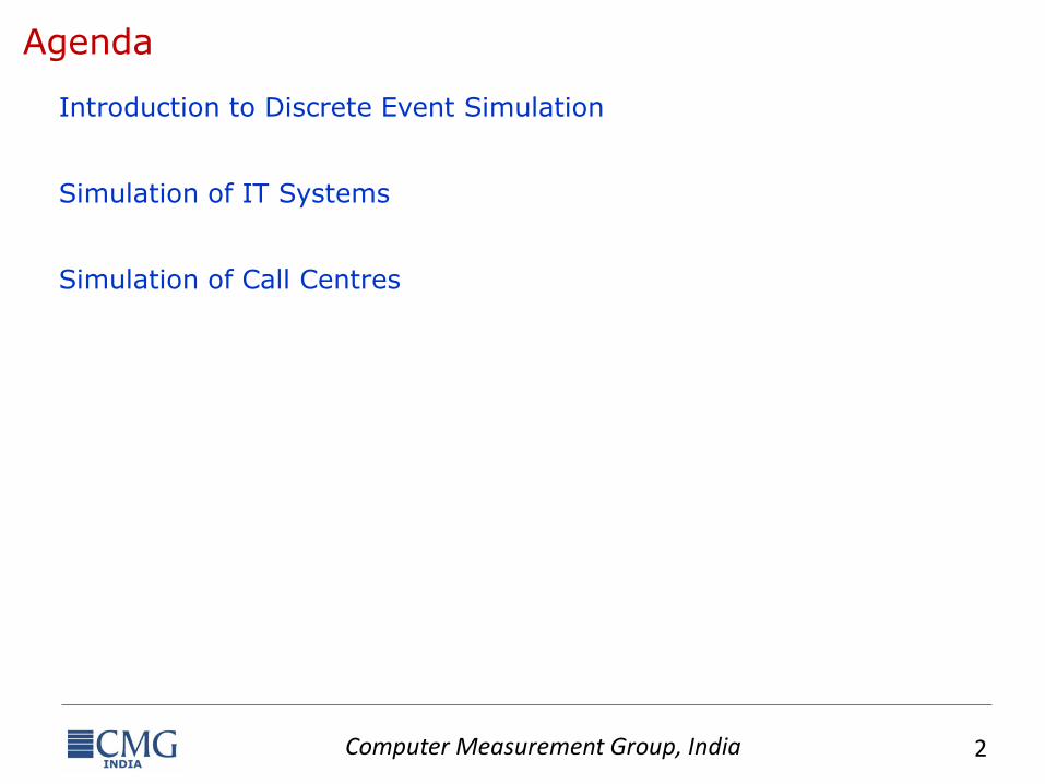
Performance Modelling Techniques

Analytical Modelling

• Abstract the system into network of queues

• Establish queuing relationships using mathematical expressions

• Solution based on

• Operational laws

• Queuing theory

• Markov Chains

• Stochastic Petri nets

Simulation Modelling

• Abstract the system into network of resources

• Relationships and interaction between resources modelled using “code”

• Interaction between model in a simulation environment used to get the desired data


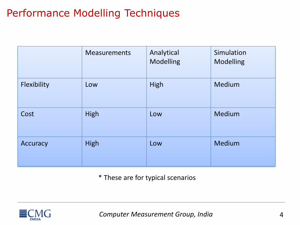
Performance Modelling Techniques

Measurements Analytical Modelling

Simulation Modelling

Flexibility Low High Medium

Cost High Low Medium

Accuracy High Low Medium

* These are for typical scenarios


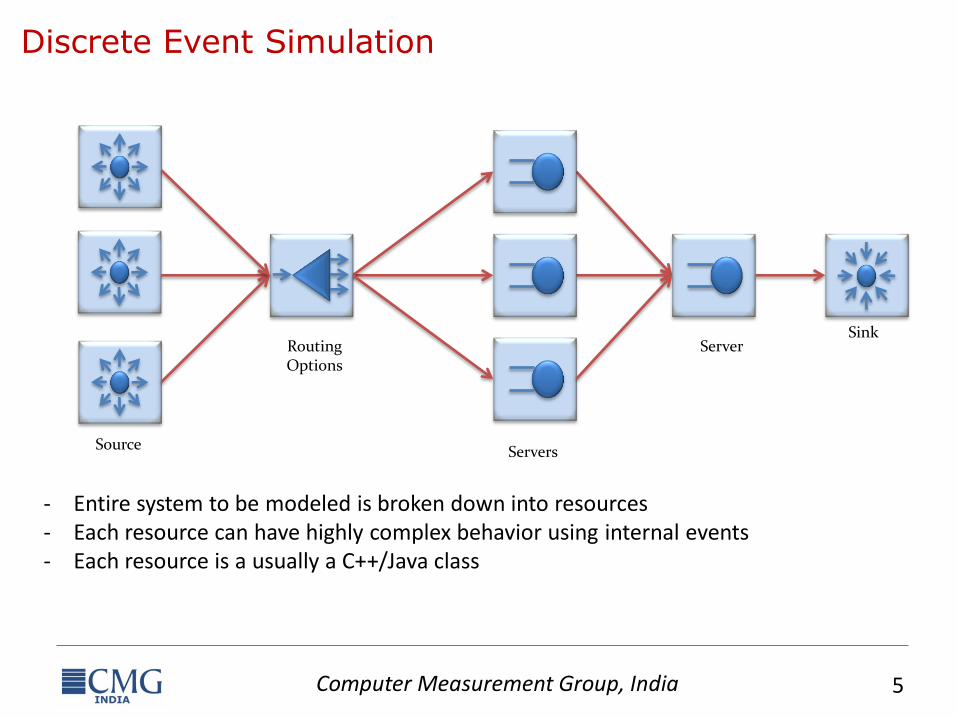
Discrete Event Simulation

Sink Routing

Options

Source Servers

Server

- Entire system to be modeled is broken down into resources - Each resource can have highly complex behavior using internal events - Each resource is a usually a C++/Java class


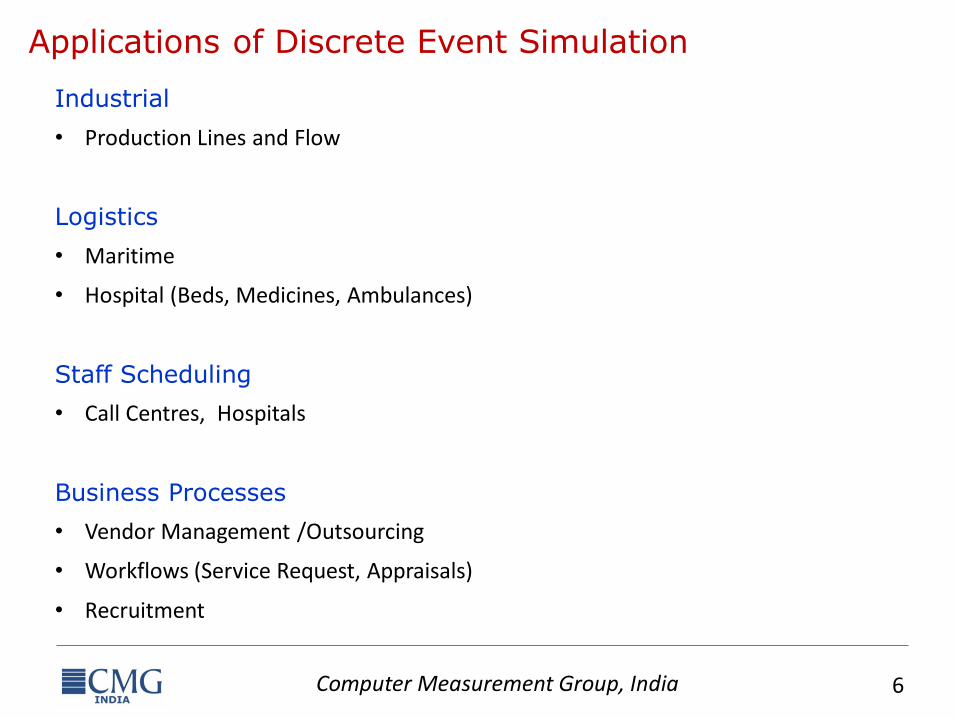
Applications of Discrete Event Simulation

Industrial

• Production Lines and Flow

Logistics

• Maritime

• Hospital (Beds, Medicines, Ambulances)

Staff Scheduling

• Call Centres, Hospitals

Business Processes

• Vendor Management /Outsourcing

• Workflows (Service Request, Appraisals)

• Recruitment


DES for Sizing/Design Decisions


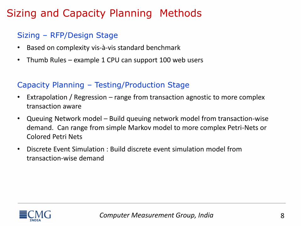
Sizing and Capacity Planning Methods

Sizing – RFP/Design Stage

• Based on complexity vis-à-vis standard benchmark

• Thumb Rules – example 1 CPU can support 100 web users

Capacity Planning – Testing/Production Stage

• Extrapolation / Regression – range from transaction agnostic to more complex transaction aware

• Queuing Network model – Build queuing network model from transaction-wise demand. Can range from simple Markov model to more complex Petri-Nets or Colored Petri Nets

• Discrete Event Simulation : Build discrete event simulation model from transaction-wise demand


Problem Statement

Sizing

• Large factor of safety has to be kept when using relative complexity / thumb rules

Can we use more sophisticated techniques

• Improve sizing accuracy at RFP stage

• Influence design decisions at RFP/Design stage


Approach

Create Building Block Library

• Demand of CPU/memory/disk/network

Build Simulation Model

Run the Simulation

• Define workload

• Define transactions with respect to building blocks

• Simulate/Do what-if


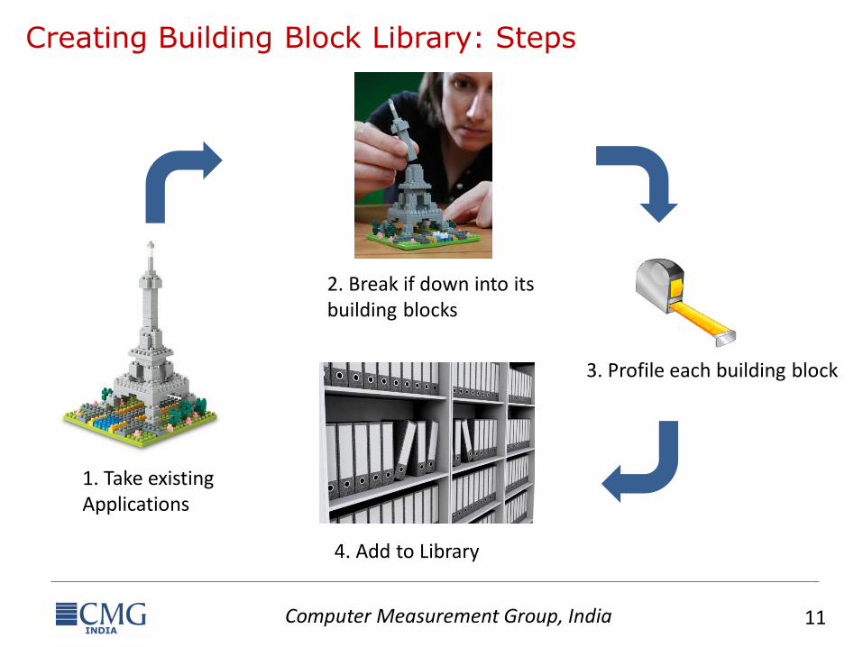
Creating Building Block Library: Steps

1. Take existing Applications

2. Break if down into its building blocks

3. Profile each building block

4. Add to Library


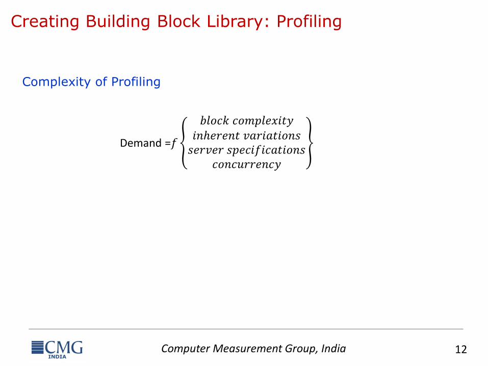
Creating Building Block Library: Profiling

Complexity of Profiling

Demand =𝑓

𝑏𝑙𝑜𝑐𝑘 𝑐𝑜𝑚𝑝𝑙𝑒𝑥𝑖𝑡𝑦𝑖𝑛ℎ𝑒𝑟𝑒𝑛𝑡 𝑣𝑎𝑟𝑖𝑎𝑡𝑖𝑜𝑛𝑠

𝑠𝑒𝑟𝑣𝑒𝑟 𝑠𝑝𝑒𝑐𝑖𝑓𝑖𝑐𝑎𝑡𝑖𝑜𝑛𝑠𝑐𝑜𝑛𝑐𝑢𝑟𝑟𝑒𝑛𝑐𝑦


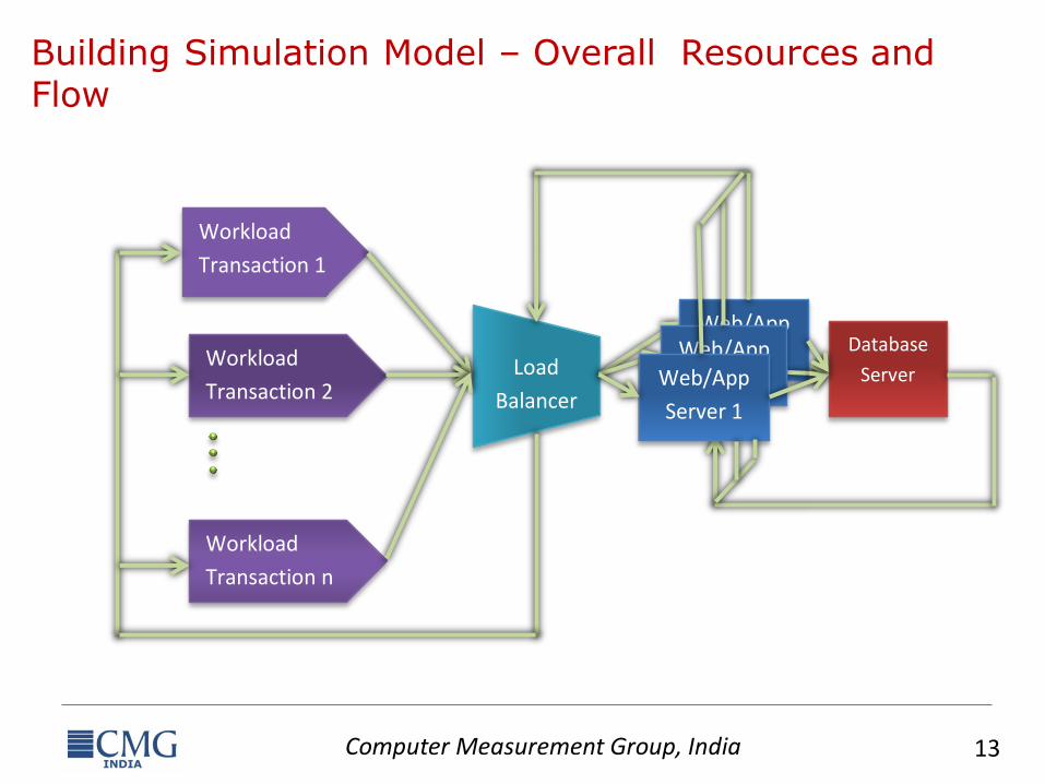
Building Simulation Model – Overall Resources and Flow

Workload

Transaction 1

Workload

Transaction 2

Workload

Transaction n

Load

Balancer

Web/App

Server 1 Database

Server Web/App

Server 2 Web/App

Server 1


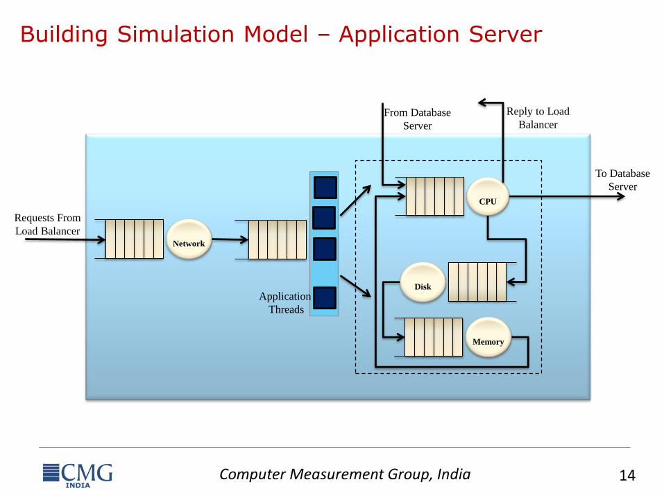
Building Simulation Model – Application Server

To Database

Server

CPU

Disk

Requests From

Load Balancer

Application

Threads

From Database

Server

Reply to Load

Balancer

Network

Memory


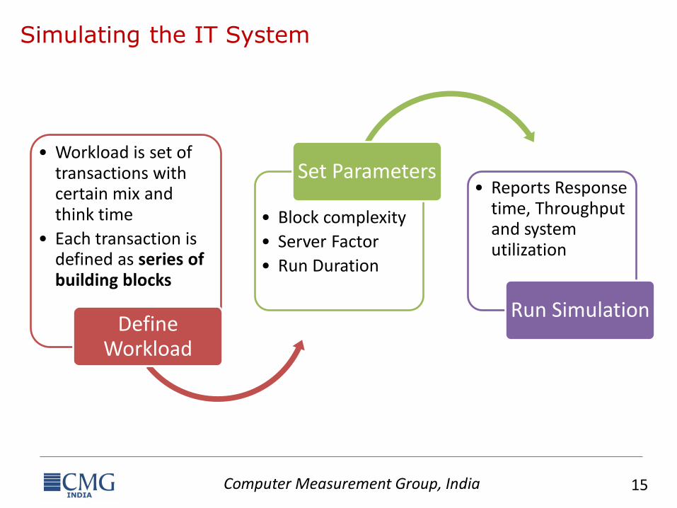
Simulating the IT System

• Workload is set of transactions with certain mix and think time

• Each transaction is defined as series of building blocks

Define Workload

• Block complexity

• Server Factor

• Run Duration

Set Parameters • Reports Response

time, Throughput and system utilization

Run Simulation


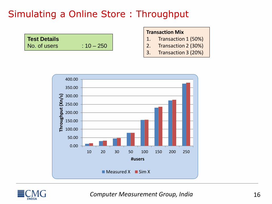
Simulating a Online Store : Throughput

Transaction Mix 1. Transaction 1 (50%) 2. Transaction 2 (30%) 3. Transaction 3 (20%)

Test Details

No. of users : 10 – 250

0.00

50.00

100.00

150.00

200.00

250.00

300.00

350.00

400.00

10 20 30 50 100 150 200 250

Thro

ugh

pu

t (X

n/s

)

#users

Measured X Sim X


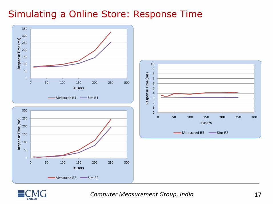
Simulating a Online Store: Response Time

0

50

100

150

200

250

300

350

0 50 100 150 200 250 300

Re

spo

nse

Tim

e (

ms)

#users

Measured R1 Sim R1

0

1

2

3

4

5

6

7

8

9

10

0 50 100 150 200 250 300

Res

pons

e Ti

me

(ms)

#users

Measured R3 Sim R3

0

50

100

150

200

250

300

0 50 100 150 200 250 300

Re

spo

nse

Tim

e (

ms)

#users

Measured R2 Sim R2


DES for Call Centre Manpower Planning


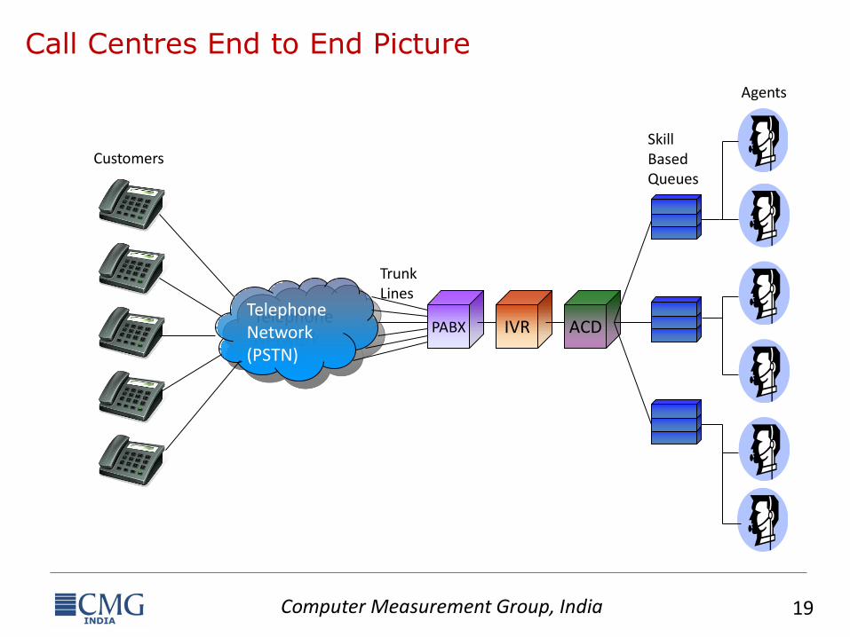
Call Centres End to End Picture

Telephone Network (PSTN)

PABX IVR ACD

Skill Based Queues

Customers

Agents

Trunk Lines


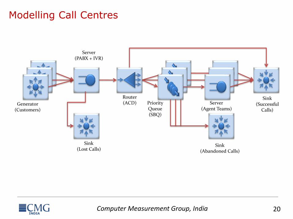
Modelling Call Centres

Generator (Customers)

Sink (Lost Calls)

Sink (Abandoned Calls)

Sink (Successful

Calls)

Server (Agent Teams)

Server (PABX + IVR)

Router (ACD) Priority

Queue (SBQ)


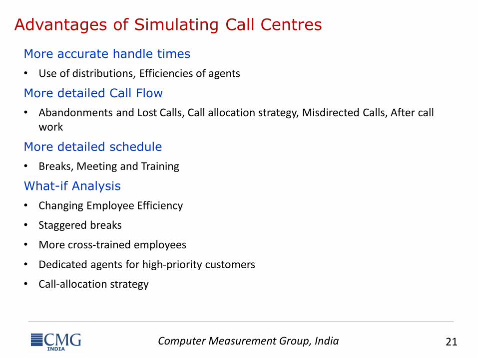
Advantages of Simulating Call Centres

More accurate handle times

• Use of distributions, Efficiencies of agents

More detailed Call Flow

• Abandonments and Lost Calls, Call allocation strategy, Misdirected Calls, After call work

More detailed schedule

• Breaks, Meeting and Training

What-if Analysis

• Changing Employee Efficiency

• Staggered breaks

• More cross-trained employees

• Dedicated agents for high-priority customers

• Call-allocation strategy


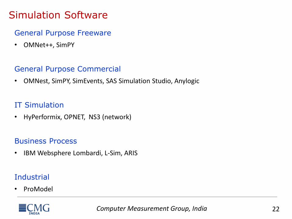
Simulation Software

General Purpose Freeware

• OMNet++, SimPY

General Purpose Commercial

• OMNest, SimPY, SimEvents, SAS Simulation Studio, Anylogic

IT Simulation

• HyPerformix, OPNET, NS3 (network)

Business Process

• IBM Websphere Lombardi, L-Sim, ARIS

Industrial

• ProModel


Q and A


APPENDIX


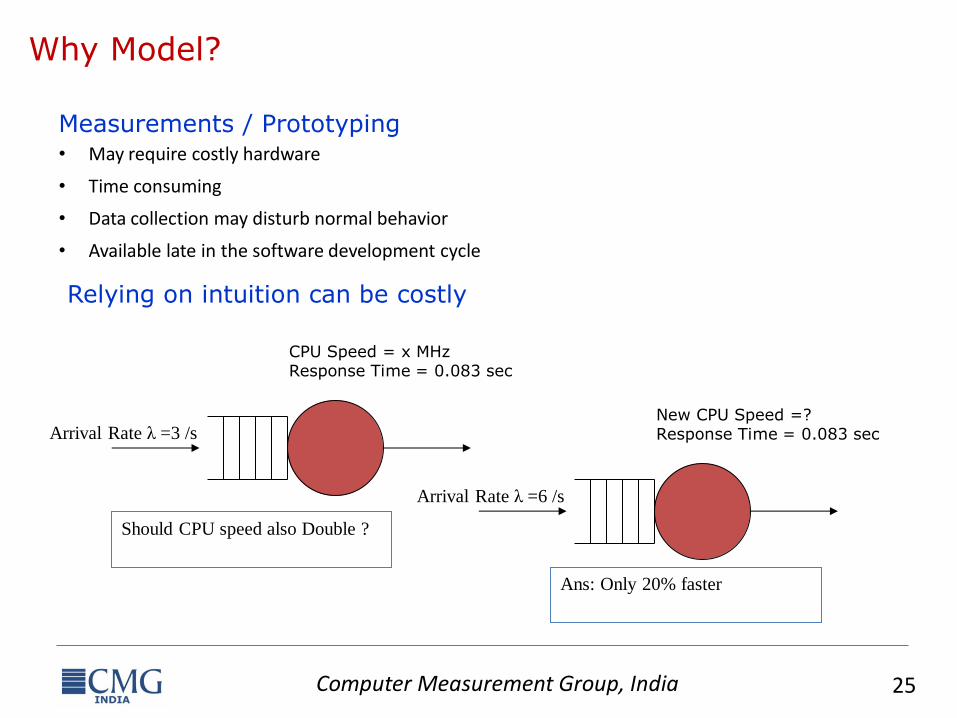
Why Model?

Measurements / Prototyping • May require costly hardware

• Time consuming

• Data collection may disturb normal behavior

• Available late in the software development cycle

Relying on intuition can be costly

Arrival Rate λ =3 /s

CPU Speed = x MHz Response Time = 0.083 sec

Arrival Rate λ =6 /s

New CPU Speed =? Response Time = 0.083 sec

Should CPU speed also Double ?

Ans: Only 20% faster


Analytical or Simulation

Analytical:

• Best for steady state analysis

• Cheaper to build

• Usually faster to solve

• Solution time does not depend on rare events

Simulation:

• Best when there is time varying behaviour

• More expensive to build and takes time to solve

• Solution time can be very high if there are rare events

• Move from Analytical to Simulation when

• The model is very complex with many variables and interacting components

• The underlying variables relationships are nonlinear

• The model contains random distributions


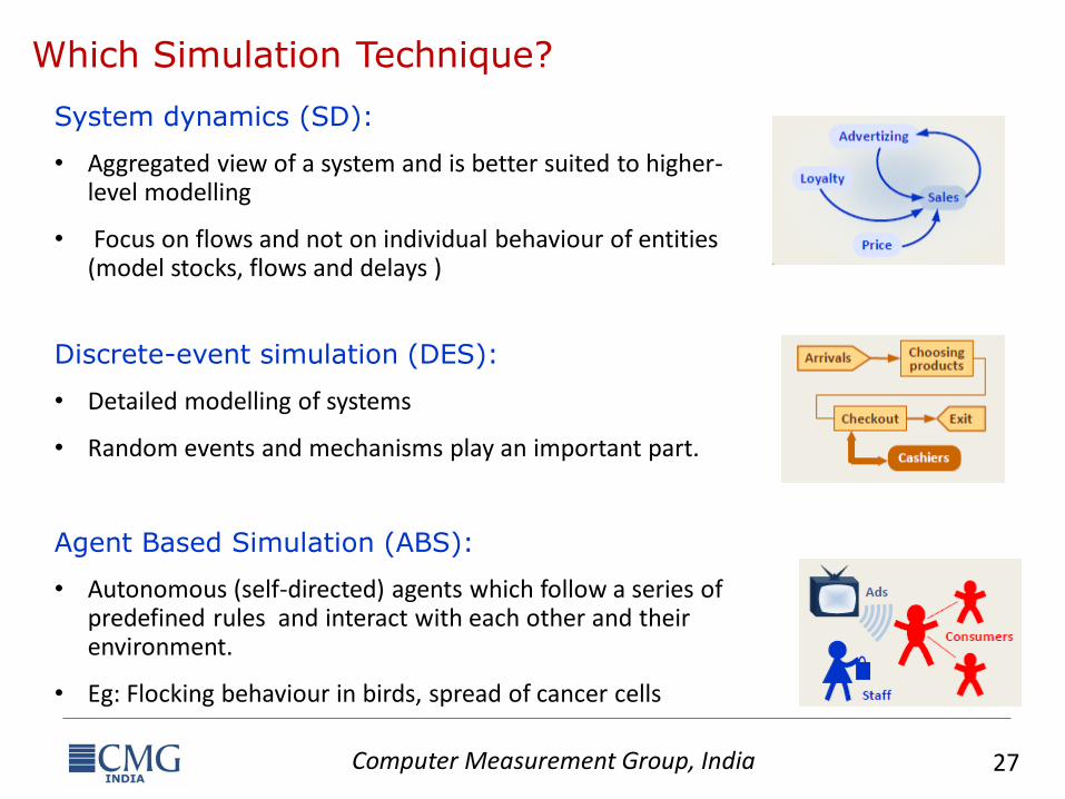
Which Simulation Technique?

System dynamics (SD):

• Aggregated view of a system and is better suited to higher-level modelling

• Focus on flows and not on individual behaviour of entities (model stocks, flows and delays )

Discrete-event simulation (DES):

• Detailed modelling of systems

• Random events and mechanisms play an important part.

Agent Based Simulation (ABS):

• Autonomous (self-directed) agents which follow a series of predefined rules and interact with each other and their environment.

• Eg: Flocking behaviour in birds, spread of cancer cells


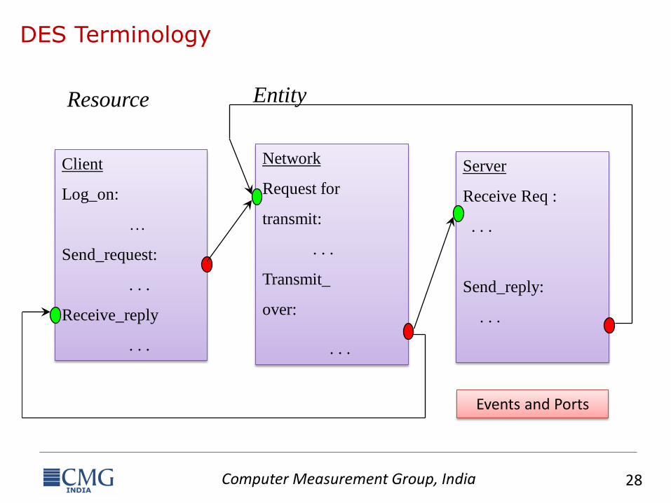
DES Terminology

Client

Log_on:

…

Send_request:

. . .

Receive_reply

. . .

Network

Request for

transmit:

. . .

Transmit_

over:

. . .

Server

Receive Req :

. . .

Send_reply:

. . .

Resource Entity

Events and Ports


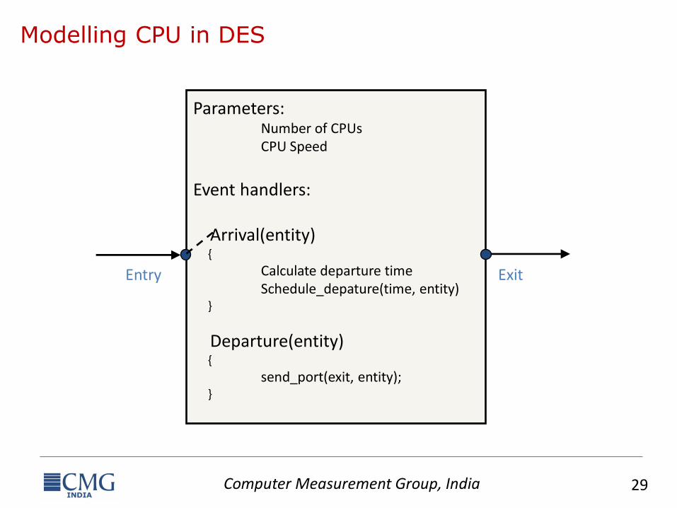
Modelling CPU in DES

Parameters: Number of CPUs CPU Speed

Event handlers: Arrival(entity) {

Calculate departure time Schedule_depature(time, entity) }

Departure(entity) {

send_port(exit, entity); }

Entry Exit


Modelling CPU in DES

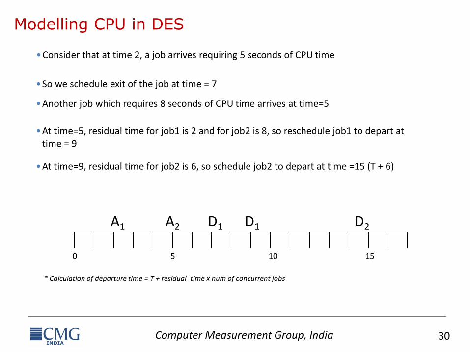
•Consider that at time 2, a job arrives requiring 5 seconds of CPU time

0 5 10 15

A1

•So we schedule exit of the job at time = 7

•Another job which requires 8 seconds of CPU time arrives at time=5

D1 A2

•At time=5, residual time for job1 is 2 and for job2 is 8, so reschedule job1 to depart at time = 9

D1

•At time=9, residual time for job2 is 6, so schedule job2 to depart at time =15 (T + 6)

D2

* Calculation of departure time = T + residual_time x num of concurrent jobs


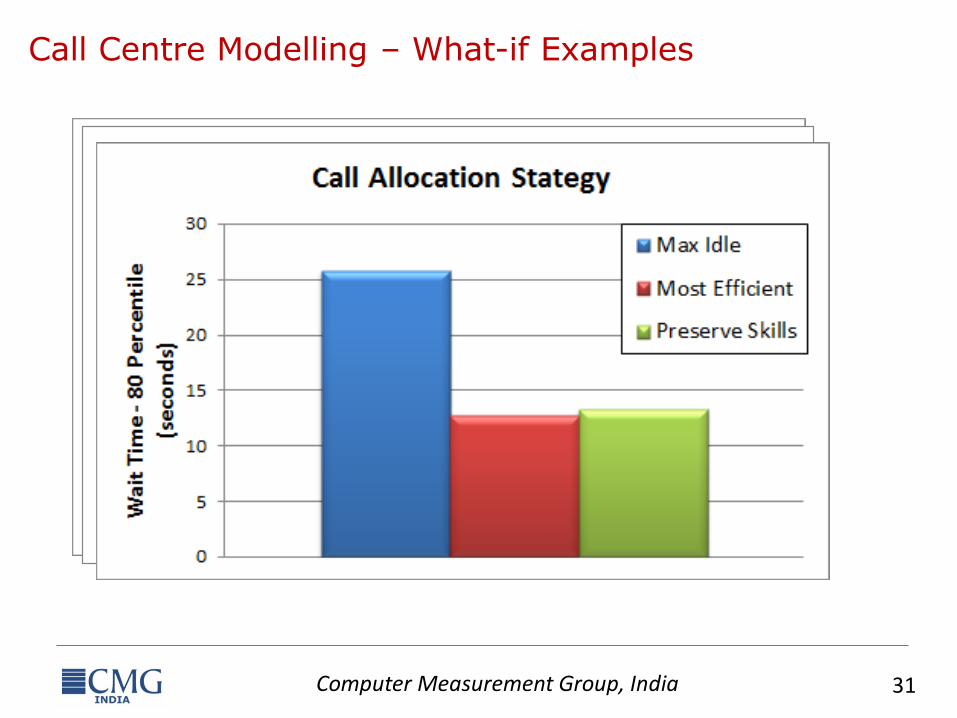
Call Centre Modelling – What-if Examples

0

20

40

60

80

100

120

Wai

t Ti

me

-80

Per

cen

tile

(se

con

ds)

Impact of Distribution

exp(180)

logn(5.0679,0.5)

logn(4.4117,1.25)


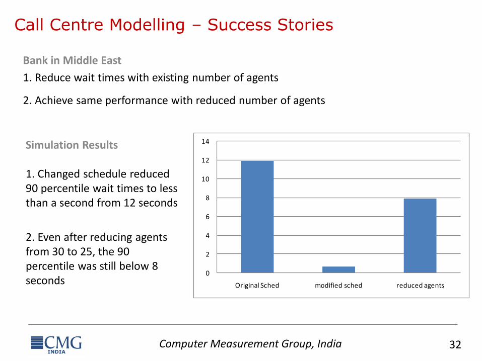
Call Centre Modelling – Success Stories

Bank in Middle East

1. Reduce wait times with existing number of agents

2. Achieve same performance with reduced number of agents

0

2

4

6

8

10

12

14

Original Sched modified sched reduced agents

Simulation Results 1. Changed schedule reduced 90 percentile wait times to less than a second from 12 seconds

2. Even after reducing agents from 30 to 25, the 90 percentile was still below 8 seconds

Documents

Performance Modelling Using Discrete Event … Measurement Group, India 1 Performance Modelling Using Discrete Event Simulation Benny Mathew Tata Consultancy Services [email protected]