Embed Size (px)
Citation preview

Power Balance in a Helicon Plasma Source for Space Propulsion
Daniel B. White Jr., Manuel Martinez-Sanchez
June 2008 SSL # 9-08


1
Power Balance in a Helicon Plasma Source for Space Propulsion
Daniel B. White Jr., Manuel Martinez-Sanchez
June 2008 SSL # 9-08
This work is based on the unaltered text of the thesis by Daniel B. White Jr. submitted to the
Department of Aeronautics and Astronautics in partial fulfillment of the requirements for the
degree of Master of Science at the Massachusetts Institute of Technology.

2
3
Power Balance in a Helicon Plasma Source for Space Propulsion
by
Daniel B. White Jr.
Submitted to the Department of Aeronautics and Astronautics
on May 23, 2008, in partial fulfillment of the
requirements for the degree of
MASTER OF SCIENCE IN AERONAUTICS AND ASTRONAUTICS
Abstract
Electric propulsion systems provide an attractive option for various spacecraft propulsion
applications due to their high specific impulse. The power balance of an electric thruster based
on a helicon plasma source is presented. The power balance is shown to be comprised of several
variables, including the RF power supplied to the system, dissipative losses in transmission
hardware, losses in the neutral confinement tube, uncoupled RF radiation, ionization power, and
plume output power.
A thermal model for the neutral confinement tube is presented whereby heat flux may be derived
from thermal response data. Numerical simulation and experimental benchmarking are
employed to validate this thermal model.
A mapping of power consumption is presented. Comparison with experimental parameters
indicates that 97% of the power supplied to the system is accounted for, suggesting that primary
loss mechanisms have been identified. Avenues for improving the performance of the thruster,
based on these data, are presented.
Thesis Supervisor: Manuel Martinez-Sanchez
Title: Professor of Aeronautics and Astronautics

4

5
Acknowledgements
This work was performed primarily under contract #RS060213 with ARFL/ERC/Edwards as part
of the Experimental Study of the Mini-Helicon Thruster program. The author gratefully thanks
Dr. Arthur Gelb for his generous support that enabled this research.

6

7
Contents
1 Introduction 16
1.1 Historical Context..................................................................................................16
1.2 Helicon Plasma Source..........................................................................................23
1.2.1 Source Properties.......................................................................................23
1.2.2 Acceleration Mechanism...........................................................................24
1.3 Helicon Plasma Thruster Design...........................................................................25
1.3.1 Evolution of the mHTX Design.................................................................25
1.3.2 RF Circuit..................................................................................................25
1.3.3 Magnetic Structure.....................................................................................26
1.3.4 Confinement Structure...............................................................................28
1.3.5 Propellant Feed System..............................................................................29
2 Power Balance 30
2.1 Microscopic Loss Effects.......................................................................................30
2.1.1 Transmission Loss.....................................................................................30
2.1.2 Ionization & Excitation..............................................................................33
8
2.1.3 Neutral Flux...............................................................................................36
2.1.4 Radial Plasma Diffusion............................................................................36
2.1.5 Non-Ideal Utilization.................................................................................37
2.1.6 RF Irradiance.............................................................................................37
2.1.7 Transmitted Radiation................................................................................37
2.1.8 Plume Power..............................................................................................39
2.2 Macroscopic Effects...............................................................................................40
2.2.1 Transmission Hardware Heating...................................................................40
2.2.1 Confinement Tube Heating...........................................................................40
2.2.2 Plume Power.................................................................................................41
2.2.3 RF Flux Measurements.................................................................................41
2.3 Power Balance.......................................................................................................41
3 Benchmarking 43
3.1 Analytic Approach.................................................................................................43
3.2 Numerical Simulation............................................................................................49
3.2.1 Exact Solution............................................................................................54
3.2.2 Linearization..............................................................................................56
3.3 Measurements........................................................................................................59
4 mHTX Power Measurements 62
4.1 Transmission Hardware Heating............................................................................62
4.1.1 Coaxial Transmission Cable......................................................................63
4.1.2 Antenna......................................................................................................64

9
4.1.3 Vacuum Feed Through..............................................................................66
4.2 Ionization Power....................................................................................................67
4.3 Confinement Tube Heating....................................................................................68
4.4 Plume Power..........................................................................................................86
4.5 RF Flux Measurements..........................................................................................86
5 Conclusion 87
5.1 Power Balance Tabulation.....................................................................................87
5.2 Improving Performance.........................................................................................88
5.3 Recommendations for Future Work.......................................................................89
A Helicon Thruster Control Software 91
B Finite Difference Modeling Code 101
C Photos of Experimental Hardware 104
10
List of Figures
1-1 RF circuit for the helicon experiment in the MIT SPL. The transmission line is
represented with characteristic impedance ZT. The impedance matching network is
formed by Z1 & Z2. C1 & C2 form a voltage-sensing network. T1 is used for current
sensing. Load impedance is dynamic, and related to the character of the plasma
discharge. .........................................................................................................................26
1-2 SPL propellant feed system for mHTX. Current experimental work uses argon
propellant. ........................................................................................................................29
2-1 Log-log plot of skin depth and characteristic resistance as a function of operating
frequency. Note that the characteristic resistance has units of [Ω·m2 / m
2]. ...................32
2-2 Ideal power required for full ionization of several noble gas propellants. Power required
for ionization is governed by εi, the ionization energy for the species.
............................................................................................................................................34
2-3 Brusa model for the total ionization and total excitation cross-sections in argon as a
function of incident electron energy. The ionization cross section reaches a maximum
value of Qi ≈ 4.4 x 10⁻²⁰ m
2 at ε ≈ 40 eV. The excitation cross section reaches a
maximum value of QEX = 7.927 x 10⁻²¹ m
2 at ε ≈ 50 eV. ................................................35
11
2-4 Radiation transmission characteristics of fused silica. Transparency increases very
sharply at approximately 200 nm, and declines sharply above 4000 nm. .......................38
2-5 Thrust versus mass flow rate measurement for PRF = 635 W, B0 = 1540 G as a function of
mass flow rates of argon. .................................................................................................40
3-1 Cutaway of particle confinement tube outfitted with helical resistive element. Resistor is
wound from 22 AWG Nichrome-A stock. Total wound length is 23 cm without
compression. Resistance is RC ≈ 7.4 Ω. ..........................................................................47
3-2 Thermocouple placement along confinement tube. Five K-type thermocouples are
bonded at equal intervals along the 40 cm length. ...........................................................48
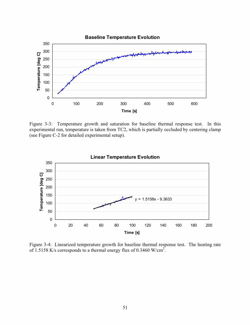
3-3 Temperature growth and saturation for baseline thermal response test. In this
experimental run, temperature is taken from TC2, which is partially occluded by the
centering clamp (see Figure C-2 for detailed experimental setup). .................................51
3-4 Linearized temperature growth for baseline thermal response test. The heating rate of
1.5158 K/s corresponds to a thermal energy flux of 0.3460 W/cm2. ...............................51
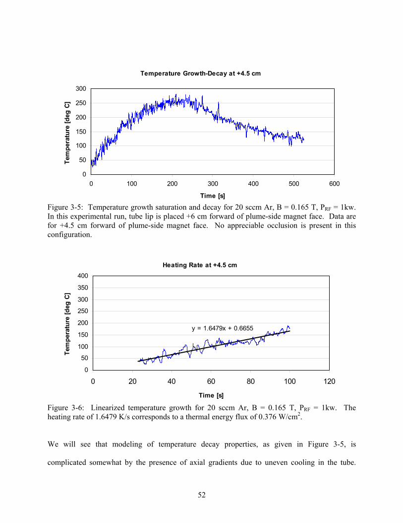
3-5 Temperature growth saturation and decay for 20 sccm Ar, B = 0.165 T, PRF = 1kw. In
this experimental run, tube lip is placed +6 cm forward of plume-side magnet face. Data
are for +4.5 cm forward of plume-side magnet face. No appreciable occlusion is present
in this configuration. ........................................................................................................52
3-6 Linearized temperature growth for 20 sccm Ar, B = 0.165 T, PRF = 1 kw. The heating
rate of 1.6479 K/s corresponds to a thermal energy flux of 0.376 W/cm2. .....................52
3-7 Real and simulated thermal response of the neutral confinement tube during the baseline
experimental run. Simulated curve is given for PIN = 3460 W/m2 and α = 0.55. ...........55
12
3-8 Exact solution for finite-difference simulated temperature growth and decay. Simulated
curve uses PIN = 3762 W/m2, with blackbody parameter α = 0.58. .................................55
3-9 Simulation of a baseline thermal response curve using a linearization scheme. Coverage
of the thermocouple area by retaining clamp in this experiment drives down the gray
body parameter. This plot corresponds to PIN = 3460 W/m2, and α = 0.55. ...................57
3-10 Simulated temperature growth and decay using a linearization scheme. Simulated curve
uses PIN = 3762 W/m2, with blackbody parameter α = 0.58. ...........................................57
3-11 Temperature evolution of the resistive element and confinement tube. Power applied to
the system is 16.45 W. At this heating rate, thermal response of the outer surface of the
source tube requires approximately 25 s. .........................................................................59
3-12 Linear fit of temperature data. The data subset is taken immediately following the onset
of thermal response on the confinement tube outer surface. Operation below 80 ºC
ensures that radiative effects can be neglected. ...............................................................60
4-1 Helicon antenna temperature evolution over a two-minute run. Thermocouple is bonded
directly to antenna in this experimental run. Excessive noise in the temperature signal is
presumably caused by RF coupling to the thermocouple. Projected heating rate is
presented in red. ...............................................................................................................64
4-2 Antenna heating rate extracted from a series of points following application of an RF
pulse with duration approximately 20 s. Hold times following pulses are typically less
than 10 seconds. Heating rates are shown in red. ...........................................................65
4-3 Temperature growth associated with the feed though outer conductor. These data are
taken 0.5 m from the vacuum chamber RF feed-through flange. ....................................66
13
4-4 Temperature response of the neutral particle confinement tube. Operating conditions
during this run are PFOR = 1.19 kW in argon at 10 sccm, with field strength B = 0.2T.
The slope indicated for the -16 cm position corresponds to a heat flux of 2.58 W/cm2. 68
4-5 Linearized temperature plots along the length of the neutral confinement tube. All plots
correspond to input power PRF = 590 W, B = 0.2 T, and a flow rate of 10 sccm. ......70-72
4-6 Linearized temperature plots along the length of the neutral confinement tube. All plots
correspond to an input power PRF = 590 W, B = 0.2 T, and a flow rate of 20 sccm. 73-75
4-7 Linearized temperature plots along the length of the neutral confinement tube. All plots
correspond to an input power PRF = 590 W, B = 0.2 T, and a flow rate of 40 sccm. 76-78
4-8 Linearized temperature plots along the length of the neutral confinement tube. All plots
correspond to an input power PRF = 590 W, B = 0.09 T, and a flow rate of 10 sccm. 79-81
4-9 Heat flux to the walls of the neutral particle confinement tube. Operating conditions are
PFOR = 0.59 kW in argon at (a) 10 sccm, (b) 20 sccm, and (c) 40 sccm with field strength
B = 0.2T. ..........................................................................................................................83
4-10 Thermal response of the neutral particle confinement tube. Operating conditions during
this run are PFOR = 0.59 kW in argon 20 sccm, with (a) B = 0.09T, and (b) B = 0.2T. ...84
4-11 Axial magnetic field strength for the electromagnet assembly associated with the mHTX.
Note that, as in the figures for axial heat flux, the plume-side electromagnetic face
corresponds to x = 0 cm. Propellant is injected upstream at x = 40 cm, travels in the
xe− direction, and is exhausted at x = 0 cm. ...................................................................85
A-1 RF power supply control VI. This graphical user interface (GUI) is used to control the
RFPP RF-10S/PWT 1.2 kW 13.56 MHz power supply. .................................................93
A-2 Block diagram illustrating the control logic for the RFPS GUI. .....................................94
14
A-3 Magnet control VI. This GUI is used to control the Agilent N5761A 6V 180A 1080W
power supply supplying the magnetic field for the mHTX. ............................................95
A-4 Block diagram for the LVPS GUI. ..................................................................................96
A-5 Propellant flow rate control VI. Used to control the propellant flow control loop. .......97
A-6 Block diagram for the propellant flow rate control GUI. ................................................98
A-7 Temperature measurement VI. This VI is used to acquire the temperature measurements
presented in this work. .....................................................................................................99
A-8 Block diagram for temperature acquisition GUI. ..........................................................100
B-1 Code for computing the exact solution to the fourth order polynomial expression for Ti+1
in finite-difference modeling of the neutral confinement temperature evolution.
Developed using MATLAB R2006a. ............................................................................102
B-2 Code for computing the linearized approximation for Ti+1 in finite-difference modeling of
the neutral confinement temperature evolution. Developed using MATLAB R2006a. 103
C-1 Neutral confinement tube outfitted with Nichrome-A resistive element. Total wound
length is 23 cm. Resistance is R ≈ 7.4 Ω. .....................................................................105
C-2 Experimental setup for thermal baseline experiment. ....................................................105
C-3 Detail of the vacuum feed through and helicon antenna. The neutral confinement tube
fits coaxially inside the helicon antenna. Propellant gas is injected in the lower left end
and exhausted at the upper right end. .............................................................................106
C-4 mHTX setup in operation using an alumina neutral confinement tube. Thermocouple is
visible, bonded to the source tube near the exit. ............................................................106

15
List of Tables
1-1 Typical velocity increments for interplanetary and interstellar missions. .......................17
1-2 Theoretical performance of various chemical rocket propellant combinations; PC = 1000
psia; Expansion to sea level is 14.7 psia. Vacuum expansion implies Ae/At = 40
(prepared by Rocketdyne Chemical and Material Technology). .....................................18
1-3 Typical operating features for selected electric thrusters. ...............................................19
1-4 Properties of fused silica used in current neutral particle confinement tube on mHTX. 28
1-5 Properties of alumina to be used in future revision of neutral particle confinement tube on
mHTX. .............................................................................................................................28
2-1 Property data for copper. ..................................................................................................32
2-2 Property data for argon. ...................................................................................................33
2-3 Parameters for computing the total ionization and total excitation cross sections in argon.
Computed cross section is expressed as a function of electron energy. ..........................36
2-4 Vacuum wavelengths of high-intensity persistent argon spectral lines. Wavelengths are
uniformly below the transparency cutoff for quartz and will therefore contribute to
confinement tube heating. ................................................................................................38
5-1 Tabulated power for the mHTX experiment. ...................................................................88
16
Chapter 1
Introduction
The helicon plasma source has several advantages over competing technologies for producing
high density, accelerated plasma flows suitable for application to spacecraft propulsion. The
power balance associated with the mini-Helicon Thruster Experiment (mHTX) at MIT is
evaluated herein, with the goal of evaluating overall thrust efficiency and mapping avenues for
improving performance.
1.1 Historical Context
The utility of ionized gases for space propulsion has been recognized since the time of
Tsiolkovsky [1]. Robert H. Goddard informally outlined many of the principles and physical
concepts in the 1900s [2]. In the late 1920s, Oberth, building on these principles, included a
section about electric propulsion in his classic book Wege zur Raumschiffahrt [3]. The first peer-
reviewed study on the viability of electric propulsion (EP) appeared in 1948 [4], following the
development of lightweight nuclear power systems. In the United States, Ernst Stulinger did
much to develop the field of electric propulsion during the 1950s [5-7]
.
17
The first successful spaceflight of an electric thruster occurred in July 1964, when the SERT I
gridded ion engine completed a pre-programmed thrust profile during a 25 minute suborbital
flight [8]. In 1998, Deep Space 1 (DS1) was the first spacecraft to use an electric thruster for
primary propulsion [9]. The DS1, Hayabusa
[10], Smart 1
[11], and Dawn
[12] spacecraft all
illustrate the utility of electric propulsion for high-energy missions that might not otherwise be
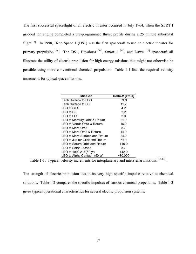
possible using more conventional chemical propulsion. Table 1-1 lists the required velocity
increments for typical space missions.
Mission Delta-V [km/s]
Earth Surface to LEO ~9.3
Earth Surface to C3 11.2
LEO to GEO 4.2
LEO to C3 3.2
LEO to LLO 3.9LEO to Mercury Orbit & Return 31.0
LEO to Venus Orbit & Return 16.0
LEO to Mars Orbit 5.7
LEO to Mars Orbit & Return 14.0
LEO to Mars Surface and Return 34.0
LEO to Jupiter Orbit and Return 64.0
LEO to Saturn Orbit and Return 110.0
LEO to Solar Escape 8.7
LEO to 1000 AU (50 yr) 142.0LEO to Alpha Centauri (50 yr) ~30,000
Table 1-1: Typical velocity increments for interplanetary and interstellar missions [13-14]
.
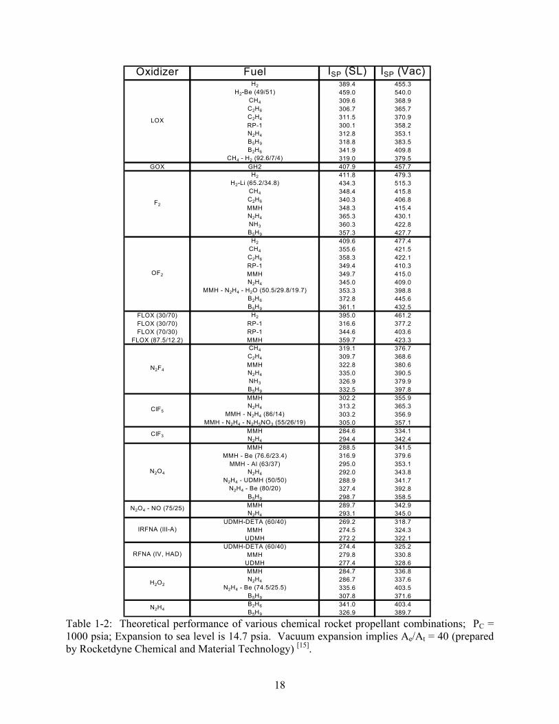
The strength of electric propulsion lies in its very high specific impulse relative to chemical
solutions. Table 1-2 compares the specific impulses of various chemical propellants. Table 1-3
gives typical operational characteristics for several electric propulsion systems.
18
Table 1-2: Theoretical performance of various chemical rocket propellant combinations; PC =
1000 psia; Expansion to sea level is 14.7 psia. Vacuum expansion implies Ae/At = 40 (prepared
by Rocketdyne Chemical and Material Technology) [15]
.
Oxidizer Fuel ISP (SL) ISP (Vac)H2 389.4 455.3
H2-Be (49/51) 459.0 540.0
CH4 309.6 368.9
C2H6 306.7 365.7
C2H4 311.5 370.9
RP-1 300.1 358.2
N2H4 312.8 353.1
B5H9 318.8 383.5
B2H6 341.9 409.8
CH4 - H2 (92.6/7/4) 319.0 379.5
GOX GH2 407.9 457.7
H2 411.8 479.3
H2-Li (65.2/34.8) 434.3 515.3
CH4 348.4 415.8
C2H6 340.3 406.8
MMH 348.3 415.4
N2H4 365.3 430.1
NH3 360.3 422.8
B5H9 357.3 427.7
H2 409.6 477.4
CH4 355.6 421.5
C2H6 358.3 422.1
RP-1 349.4 410.3
MMH 349.7 415.0
N2H4 345.0 409.0
MMH - N2H4 - H2O (50.5/29.8/19.7) 353.3 398.8
B2H6 372.8 445.6
B5H9 361.1 432.5
FLOX (30/70) H2 395.0 461.2
FLOX (30/70) RP-1 316.6 377.2
FLOX (70/30) RP-1 344.6 403.6
FLOX (87.5/12.2) MMH 359.7 423.3
CH4 319.1 376.7
C2H4 309.7 368.6
MMH 322.8 380.6
N2H4 335.0 390.5
NH3 326.9 379.9
B5H9 332.5 397.8
MMH 302.2 355.9
N2H4 313.2 365.3
MMH - N2H4 (86/14) 303.2 356.9
MMH - N2H4 - N2H5NO3 (55/26/19) 305.0 357.1
MMH 284.6 334.1
N2H4 294.4 342.4
MMH 288.5 341.5
MMH - Be (76.6/23.4) 316.9 379.6
MMH - Al (63/37) 295.0 353.1
N2H4 292.0 343.8
N2H4 - UDMH (50/50) 288.9 341.7
N2H4 - Be (80/20) 327.4 392.8
B5H9 298.7 358.5
MMH 289.7 342.9
N2H4 293.1 345.0
UDMH-DETA (60/40) 269.2 318.7
MMH 274.5 324.3
UDMH 272.2 322.1
UDMH-DETA (60/40) 274.4 325.2
MMH 279.8 330.8
UDMH 277.4 328.6
MMH 284.7 336.8
N2H4 286.7 337.6
N2H4 - Be (74.5/25.5) 335.6 403.5
B5H9 307.8 371.6
B2H6 341.0 403.4
B5H9 326.9 389.7
H2O2
N2H4
LOX
N2O4
N2O4 - NO (75/25)
IRFNA (III-A)
RFNA (IV, HAD)
N2F4
ClF5
ClF3
F2
OF2
19
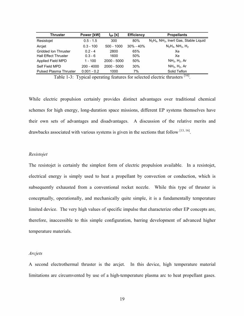
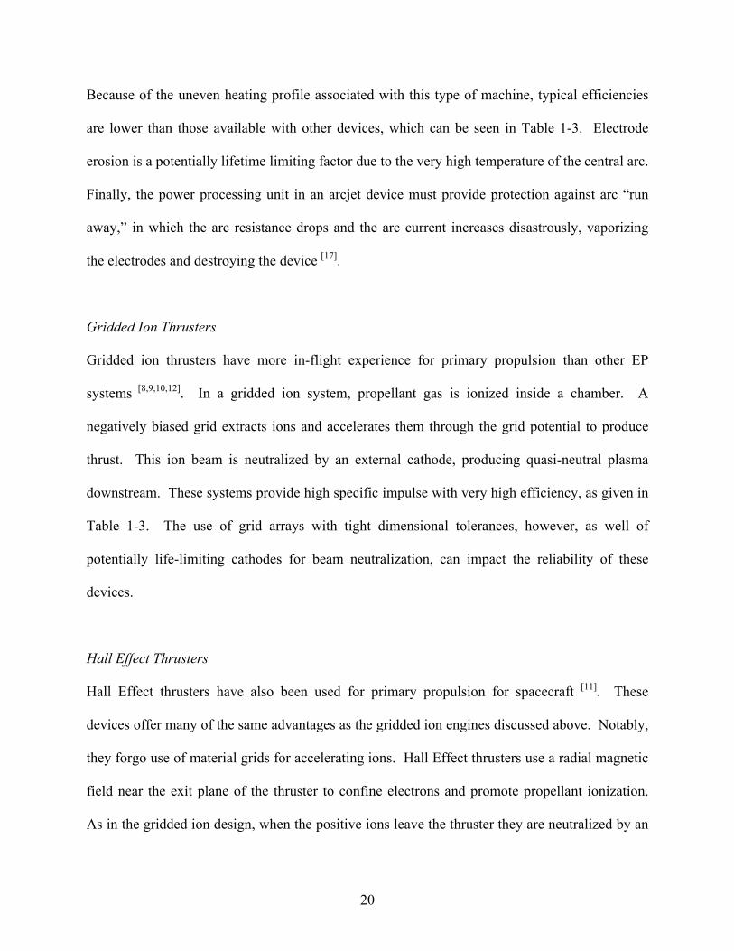
Table 1-3: Typical operating features for selected electric thrusters [16]
.
While electric propulsion certainly provides distinct advantages over traditional chemical
schemes for high energy, long-duration space missions, different EP systems themselves have
their own sets of advantages and disadvantages. A discussion of the relative merits and
drawbacks associated with various systems is given in the sections that follow [13, 16]
.
Resistojet
The resistojet is certainly the simplest form of electric propulsion available. In a resistojet,
electrical energy is simply used to heat a propellant by convection or conduction, which is
subsequently exhausted from a conventional rocket nozzle. While this type of thruster is
conceptually, operationally, and mechanically quite simple, it is a fundamentally temperature
limited device. The very high values of specific impulse that characterize other EP concepts are,
therefore, inaccessible to this simple configuration, barring development of advanced higher
temperature materials.
Arcjets
A second electrothermal thruster is the arcjet. In this device, high temperature material
limitations are circumvented by use of a high-temperature plasma arc to heat propellant gases.
Thruster Power [kW] ISP [s] Efficiency Propellants
Resistojet 0.5 - 1.5 300 80% N2H4, NH3, Inert Gas, Stable Liquid
Arcjet 0.3 - 100 500 - 1000 30% - 40% N2H4, NH3, H2
Gridded Ion Thruster 0.2 - 4 2800 65% Xe
Hall Effect Thruster 0.3 - 6 1600 50% Xe
Applied Field MPD 1 - 100 2000 - 5000 50% NH3, H2, Ar
Self Field MPD 200 - 4000 2000 - 5000 30% NH3, H2, Ar
Pulsed Plasma Thruster 0.001 - 0.2 1000 7% Solid Teflon
20
Because of the uneven heating profile associated with this type of machine, typical efficiencies
are lower than those available with other devices, which can be seen in Table 1-3. Electrode
erosion is a potentially lifetime limiting factor due to the very high temperature of the central arc.
Finally, the power processing unit in an arcjet device must provide protection against arc “run
away,” in which the arc resistance drops and the arc current increases disastrously, vaporizing
the electrodes and destroying the device [17]
.
Gridded Ion Thrusters
Gridded ion thrusters have more in-flight experience for primary propulsion than other EP
systems [8,9,10,12]
. In a gridded ion system, propellant gas is ionized inside a chamber. A
negatively biased grid extracts ions and accelerates them through the grid potential to produce
thrust. This ion beam is neutralized by an external cathode, producing quasi-neutral plasma
downstream. These systems provide high specific impulse with very high efficiency, as given in
Table 1-3. The use of grid arrays with tight dimensional tolerances, however, as well of
potentially life-limiting cathodes for beam neutralization, can impact the reliability of these
devices.
Hall Effect Thrusters
Hall Effect thrusters have also been used for primary propulsion for spacecraft [11]
. These
devices offer many of the same advantages as the gridded ion engines discussed above. Notably,
they forgo use of material grids for accelerating ions. Hall Effect thrusters use a radial magnetic
field near the exit plane of the thruster to confine electrons and promote propellant ionization.
As in the gridded ion design, when the positive ions leave the thruster they are neutralized by an
21
external cathode, yielding a quasi-neutral plume. This external cathode is, again, a potentially
lifetime limiting device. Furthermore, the ions in a Hall thruster tend to be hotter than those in
gridded machines, resulting in higher plume divergence and in chamber erosion due to ion
impingement.
Colloidal Thrusters
A device closely related to the gridded ion thruster is the colloidal thruster. In these devices,
propellant droplets with very high mass-per-unit-charge are extracted electrostatically from a
propellant dispensing capillary and accelerated through the extraction grid potential to produce
thrust. These devices are attractive in that they require no gas phase ionization, and therefore
circumvent the accompanying electrical and thermal power losses. Colloidal systems are
capable of providing very small thrust levels for very precise maneuvering. However, because of
their low thrust per dispenser, colloidal systems require very large arrays to achieve appreciable
thrust levels.
Magnetoplasmadynamic (MPD) Thrusters
An MPD is an electromagnetic thruster which uses the Lorentz force to accelerate plasma to
provide thrust. In its simplest form, it consists of a coaxial arrangement of an inner cathode and
an outer anode. The presence of conducting plasma within the channel establishes a radial
current. The azimuthal magnetic field may be applied (applied-field MPD) or, if the radial
currents are sufficiently large, self induced (self-field MPD). Because the propellant plasma is
quasi-neutral throughout, there is no need for a neutralizing external cathode. These devices are
capable of very high power densities and very high thrust density. However, the efficiency is
22
typically low, as can be seen in Table 1-3, and the very high powers at which these devices
optimize (106 - 10
7 W) are not readily achievable without nuclear power or perhaps beamed
power scenarios. Additionally, the electrodes are a potentially lifetime limiting component,
particularly due to anode starvation and the asymmetry of the discharge current.
Pulsed and Unsteady Electromagnetic Concepts
Several concepts exist for unsteady or pulse-mode electromagnetic systems, including the pulsed
plasma thruster (PPT) and the pulsed inductive thruster (PIT). Because these devices are
inherently unsteady and potentially have very high instantaneous power levels, they are prone to
high dissipative losses. In the case of the PIT, the emphasis on very short magnetic rise time
tends to drive up the conducting mass of the device, as well as the mass of the power processing
unit. PPT devices using solid propellant (usually Teflon) are very simple and robust, in spite of
their poor efficiency. The PIT has no electrodes, which are susceptible to erosion, and its
average power can be scaled up by increasing the pulse frequency.
23
1.2 Helicon Plasma Source
In 1970 a simple plasma source was discovered [18]
for producing dense plasmas by exciting
helicon waves. The utility of this plasma source for space propulsion was not exploited until
over thirty years later [19]
. Since that time, researchers throughout the world have experimentally
verified the viability of the helicon plasma source for spacecraft propulsion.
1.2.1 Source Properties
The helicon plasma source has several advantages as a source of laboratory plasma that may
potentially translate into utility as a thruster for space propulsion. First, a helicon plasma source
can operate with a wide variety of feed gases. The current experimental configuration has been
run using monatomic gases like xenon and argon, as well as molecular gases like nitrogen.
Mixed molecular species, such as air, have also been run successfully. This is advantageous for
space propulsion because it gives some flexibility in propellant selection.
Next, a helicon plasma source can produce plasmas with very high densities, approaching
1020 particles/m
3. For application to spacecraft propulsion, this means that a helicon thruster
may achieve very high thrust densities with good volumetric efficiency for the thruster as a
whole.
Finally, a helicon is an electrode-less plasma source. This eliminates the risk of
contamination of the plume with cathode material, and consequently there is a smaller risk of
contamination of the spacecraft by the plume.
24
1.2.2 Acceleration Mechanism
It is well established that bulk plasma acceleration is accomplished when the helicon wave
couples to the electron population, establishing an ambipolar electric field. Ions are in turn
accelerated by this electric field, accelerating the plasma bulk. The means by which wave
energy is transferred to the electron population with such high efficiency is still an active area of
research. It has been shown that in order for purely collisional damping to account for the
observed deposition of RF energy, the plasma must have a collision frequency at least 1000
times greater than the theoretical value [20]
. A second coupling mechanism that has been
suggested is Landau damping [21]
. Experiments indicate, however, that there are an insufficient
number of phased fast electrons in the helicon discharge for Landau damping to account for the
majority of directional coupling [22]
. Finally, Trivelpiece-Gould (TG) mode conversion has been
suggested as an alternative means of coupling helicon wave energy to the plasma [23]
. However,
analysis shows that if TG mode conversion is a dominant energy absorption mechanism in the
high-B0 plasma, such mode conversion must be occurring on the outer plasma surface only [24]
.
This is in contrast to the observed high-temperature core associated with the helicon discharge.
A final theory created to explain the efficient absorption of helicon wave energy posits that
during operation in the helicon mode, a radial plasma density gradient forms a potential well,
trapping the helicon wave, and allowing electromagnetic energy to be absorbed over the course
of repeated reflections [25]
. This theoretical framework predicts radial variation in the hot
electron population density, and data consistent with this prediction have been presented [26]
.
Despite the lack of a clear, mechanistic understanding of helicon wave damping, the
elegance of wave-coupled acceleration of plasma for space propulsion begs its exploitation. The
synergistic coupling of the ionization, heating and acceleration mechanism associated uniquely
25
with the helicon plasma source is advantageous in assuring a robust, reliable solution for future
space propulsion applications.
1.3 Helicon Plasma Thruster Design
1.3.1 Evolution of mHTX Design
The antecedents of the mHTX study at MIT lie in earlier experimental work on the first stage of
the VASIMR engine [27]
. Experimental investigation of the helicon thruster at MIT was begun in
January 2004. Since that time, several revisions of the experimental apparatus have been
implemented. Most notably, a change in the construction of the helicon antenna from braided
shielding to copper tubing has been made, and several revisions in the construction and number
of electromagnets have been effected. After preliminary implementation [28]
, spectrographic
emission data were taken for the helicon plasma source operating with argon in the helicon and
inductively coupled mode [29]
. Concurrently, preliminary work was begun in characterizing the
power balance for the helicon plasma source [30]
. Most recently, preliminary performance
metrics were gathered for the helicon plasma source, operating in its current configuration [31]
. A
more detailed description of the systems associated with the mHTX is given in the sections that
follow.
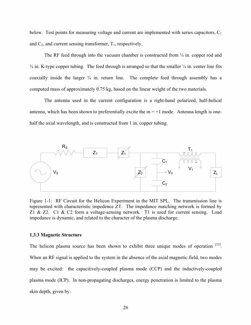
1.3.2 RF Circuit
Power is transferred from the RF power supply to the impedance matching network over
standard RG-218 coaxial cable with a characteristic impedance of 75 Ω. The matching network
is used to manually match the dynamic load impedance associated with the helicon discharge. It
is comprised of a series and shunt variable capacitor, Z1 and Z2, which can be seen in Figure 1-1
26
below. Test points for measuring voltage and current are implemented with series capacitors, C1
and C2, and current sensing transformer, T1, respectively.
The RF feed through into the vacuum chamber is constructed from ¼ in. copper rod and
¾ in. K-type copper tubing. The feed through is arranged so that the smaller ¼ in. center line fits
coaxially inside the larger ¾ in. return line. The complete feed through assembly has a
computed mass of approximately 0.75 kg, based on the linear weight of the two materials.
The antenna used in the current configuration is a right-hand polarized, half-helical
antenna, which has been shown to preferentially excite the m = +1 mode. Antenna length is one-
half the axial wavelength, and is constructed from 1 in. copper tubing.
VS
RS
ZT Z1
C2
C1
T1
V0V1
ZLZ2
Figure 1-1: RF Circuit for the Helicon Experiment in the MIT SPL. The transmission line is
represented with characteristic impedence ZT. The impedance matching network is formed by
Z1 & Z2. C1 & C2 form a voltage-sensing network. T1 is used for current sensing. Load
impedance is dynamic, and related to the character of the plasma discharge.
1.3.3 Magnetic Structure
The helicon plasma source has been shown to exhibit three unique modes of operation [32]
.
When an RF signal is applied to the system in the absence of the axial magnetic field, two modes
may be excited: the capacitively-coupled plasma mode (CCP) and the inductively-coupled
plasma mode (ICP). In non-propagating discharges, energy penetration is limited to the plasma
skin depth, given by:
27
ep
c
ωλ = . (1-1)
This expression for the skin depth is valid for e
pωω << , which is easily satisfied for the
conditions under consideration.
Alternatively, in the wave-coupled mode of operation in which an imposed axial
magnetic field is present, RF energy can penetrate to the center of the plasma, resulting in energy
deposition far from the plasma edge and offering the potential for much higher density. In the
experimental apparatus under consideration, this axial magnetic field is produced with a single
electromagnetic solenoid comprised of 162 turns of 66 mm square cross-section copper
conductor. The coil is wound on a single aluminum bobbin and has length 12 cm, outer radius of
9.5 cm, and inner radius 3.5 cm. The polyurethane insulation is rated to 200 ˚C, ultimately
limiting the full-field run time for the assembly. The total resistance of the wound copper
conductor is 0.03 Ω. The maximum current delivered to the assembly is 180 A, resulting in a
total power consumption of approximately 970 W at maximum field. Experimental
measurements using a Hall-effect sensor show that the axial magnetic field strength scales at 11
Gauss per Ampere on axis.
Future plans for the thruster magnetic assembly include the removal of the
electromagnets in favor of a high field rare-earth permanent magnet assembly.
28
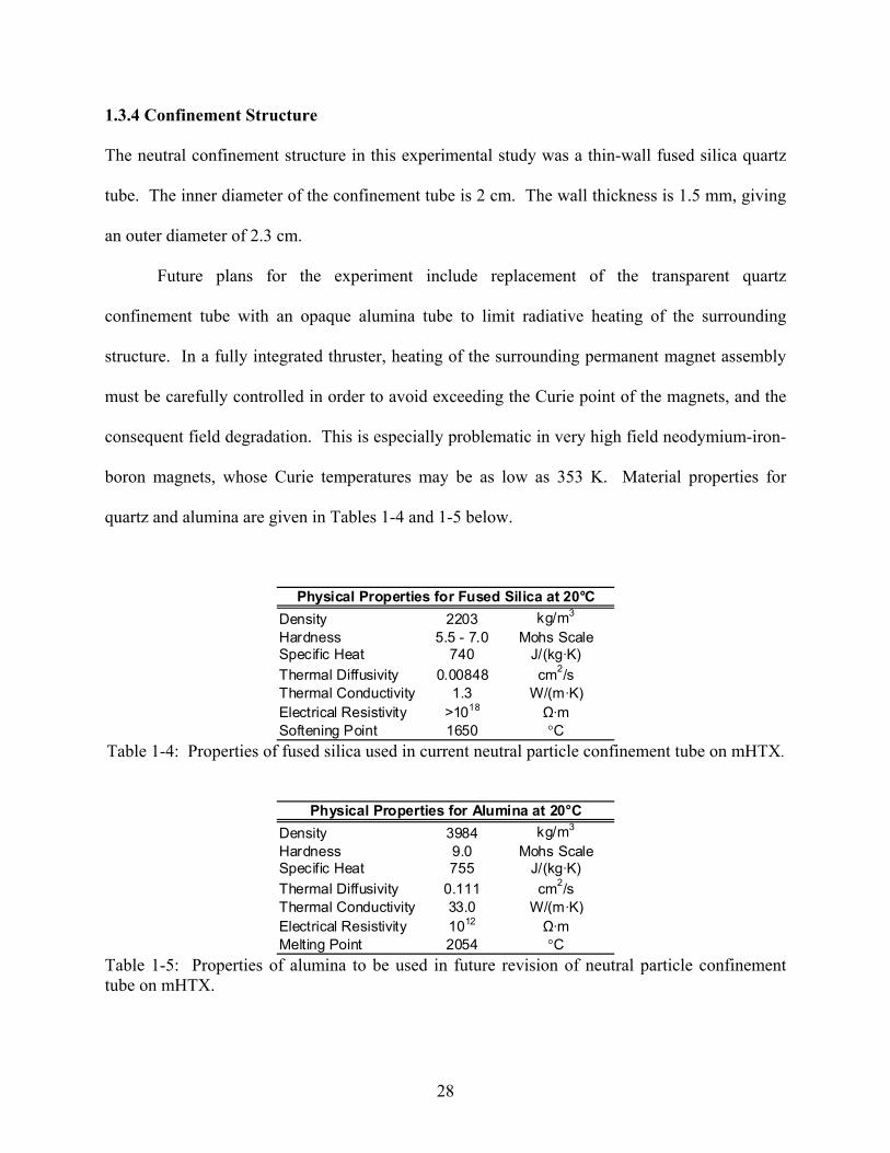
1.3.4 Confinement Structure
The neutral confinement structure in this experimental study was a thin-wall fused silica quartz
tube. The inner diameter of the confinement tube is 2 cm. The wall thickness is 1.5 mm, giving
an outer diameter of 2.3 cm.
Future plans for the experiment include replacement of the transparent quartz
confinement tube with an opaque alumina tube to limit radiative heating of the surrounding
structure. In a fully integrated thruster, heating of the surrounding permanent magnet assembly
must be carefully controlled in order to avoid exceeding the Curie point of the magnets, and the
consequent field degradation. This is especially problematic in very high field neodymium-iron-
boron magnets, whose Curie temperatures may be as low as 353 K. Material properties for
quartz and alumina are given in Tables 1-4 and 1-5 below.
Density 2203 kg/m3
Hardness 5.5 - 7.0 Mohs ScaleSpecific Heat 740 J/(kg·K)
Thermal Diffusivity 0.00848 cm2/s
Thermal Conductivity 1.3 W/(m·K)
Electrical Resistivity >1018 Ω·m
Softening Point 1650 °C
Physical Properties for Fused Silica at 20°C
Table 1-4: Properties of fused silica used in current neutral particle confinement tube on mHTX.
Density 3984 kg/m3
Hardness 9.0 Mohs ScaleSpecific Heat 755 J/(kg·K)
Thermal Diffusivity 0.111 cm2/s
Thermal Conductivity 33.0 W/(m·K)
Electrical Resistivity 1012 Ω·m
Melting Point 2054 °C
Physical Properties for Alumina at 20°C
Table 1-5: Properties of alumina to be used in future revision of neutral particle confinement
tube on mHTX.
29
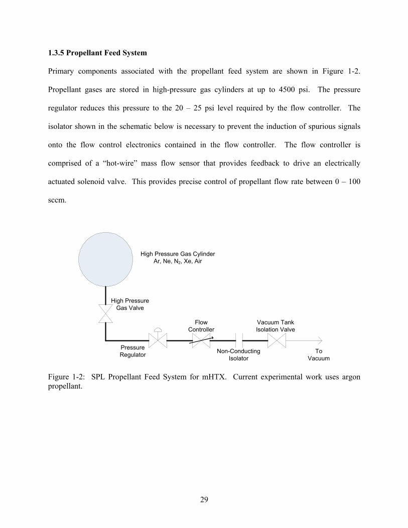
1.3.5 Propellant Feed System
Primary components associated with the propellant feed system are shown in Figure 1-2.
Propellant gases are stored in high-pressure gas cylinders at up to 4500 psi. The pressure
regulator reduces this pressure to the 20 – 25 psi level required by the flow controller. The
isolator shown in the schematic below is necessary to prevent the induction of spurious signals
onto the flow control electronics contained in the flow controller. The flow controller is
comprised of a “hot-wire” mass flow sensor that provides feedback to drive an electrically
actuated solenoid valve. This provides precise control of propellant flow rate between 0 – 100
sccm.
High Pressure Gas Cylinder
Ar, Ne, N2, Xe, Air
High Pressure
Gas Valve
Pressure
Regulator
Flow
Controller
Non-Conducting
Isolator
Vacuum Tank
Isolation Valve
To
Vacuum
Figure 1-2: SPL Propellant Feed System for mHTX. Current experimental work uses argon
propellant.
30
Chapter 2
Power Balance
In considering the overall power balance of a helicon plasma source as a thruster, there are
several small-scale effects which contribute to inefficiency and tend to increase the propellant
plasma cost-per-ion. Microscopic effects are considered. These microscopic effects are grouped
into lumped loss terms which are used to define the power balance.
2.1 Microscopic Loss Effects
2.1.1 Transmission Losses
First, power is dissipated in ohmic losses in the transmission line and antenna structure and some
power is reflected due to impedance mismatch. The RF power measured in the helicon
experiment in the SPL includes the ohmic losses in the transmission hardware. Losses in the
coaxial cable connecting the RF power supply to the impedance matching network can be
estimated. The cable is standard RG-213/U with loss –4.9 dB/100 m.
It is well known that for RF currents flowing in conductive media, current density
increases toward the surface of the conductor. In a plane conductor, the decay of current density
with increasing distance from the surface is exponential and has the form:
31
)/exp()( δdJdJ S −= . (2-1)
This is called the skin effect [33]
. The constant δ is the skin depth. From the form of Equation 2-
1, the skin depth is the distance from the conductor surface at which current density has been
reduced by a factor of e-1. For a good conductor, the skin depth is approximately given by
σµµπδ
rof
1= . (2-2)
Here σ is the electrical conductivity of the material and µr the relative permeability. This causes
the effective resistance of any solid conductor to increase with increasing frequency. For the
case of copper (σ = 5.96 x 10⁷ S/m, µr = 1) operating at 13.56 MHz, we obtain a skin depth δ ≈
17.7 µm.
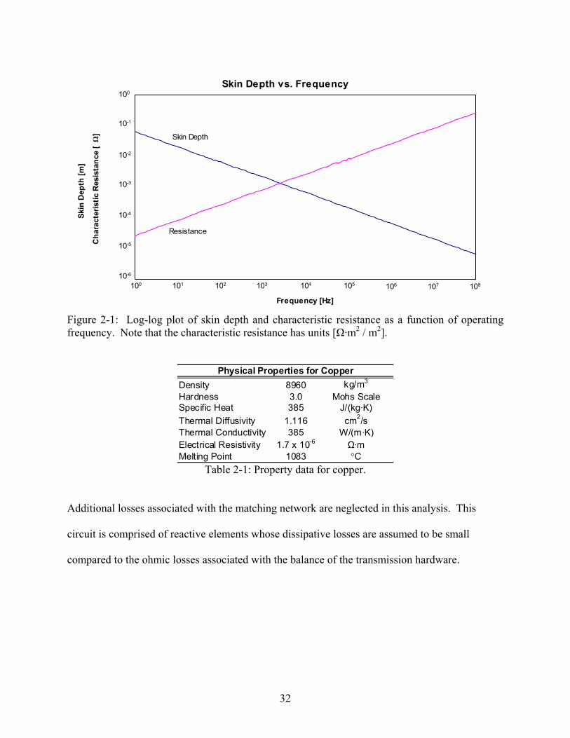
Clearly, transmission losses can be reduced somewhat by reducing operating frequency,
thereby increasing the skin depth and decreasing the resistance per unit length. Figure 2-1 below
shows the dependence of skin depth (and thus resistance) on frequency in copper.
32
Skin Depth vs. Frequency
Frequency [Hz]
Skin Depth [m]
101100 102 103 104 105 106 107
100
10-1
10-2
10-3
10-4
10-5
10-6
108
Characteristic Resistance [Ω]
Resistance
Skin Depth
Figure 2-1: Log-log plot of skin depth and characteristic resistance as a function of operating
frequency. Note that the characteristic resistance has units [Ω·m2 / m
2].
Density 8960 kg/m3
Hardness 3.0 Mohs ScaleSpecific Heat 385 J/(kg·K)
Thermal Diffusivity 1.116 cm2/s
Thermal Conductivity 385 W/(m·K)
Electrical Resistivity 1.7 x 10⁻⁶ Ω·m
Melting Point 1083 °C
Physical Properties for Copper
Table 2-1: Property data for copper.
Additional losses associated with the matching network are neglected in this analysis. This
circuit is comprised of reactive elements whose dissipative losses are assumed to be small
compared to the ohmic losses associated with the balance of the transmission hardware.
33
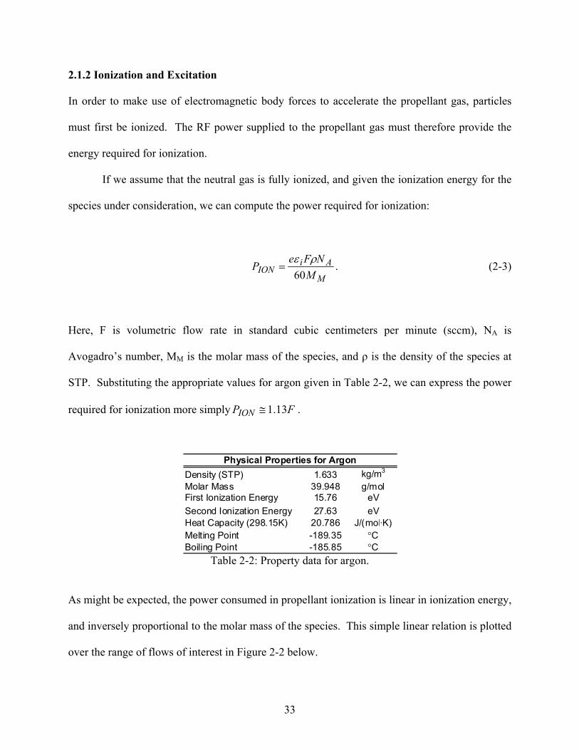
2.1.2 Ionization and Excitation
In order to make use of electromagnetic body forces to accelerate the propellant gas, particles
must first be ionized. The RF power supplied to the propellant gas must therefore provide the
energy required for ionization.
If we assume that the neutral gas is fully ionized, and given the ionization energy for the
species under consideration, we can compute the power required for ionization:
M
AiION
M
NFeP
60
ρε= . (2-3)
Here, F is volumetric flow rate in standard cubic centimeters per minute (sccm), NA is
Avogadro’s number, MM is the molar mass of the species, and ρ is the density of the species at
STP. Substituting the appropriate values for argon given in Table 2-2, we can express the power
required for ionization more simply FPION 13.1≅ .
Density (STP) 1.633 kg/m3
Molar Mass 39.948 g/molFirst Ionization Energy 15.76 eV
Second Ionization Energy 27.63 eV
Heat Capacity (298.15K) 20.786 J/(mol·K)
Melting Point -189.35 °C
Boiling Point -185.85 °C
Physical Properties for Argon
Table 2-2: Property data for argon.
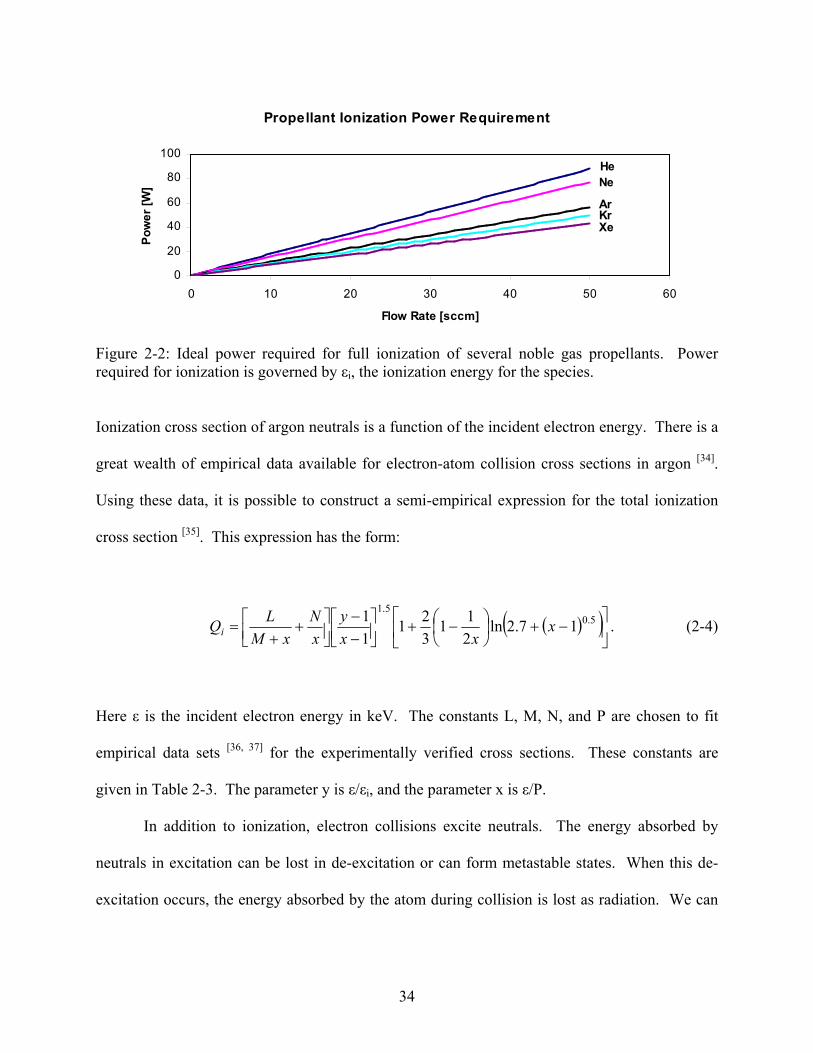
As might be expected, the power consumed in propellant ionization is linear in ionization energy,
and inversely proportional to the molar mass of the species. This simple linear relation is plotted
over the range of flows of interest in Figure 2-2 below.
34
Propellant Ionization Power Requirement
0
20
40
60
80
100
0 10 20 30 40 50 60
Flow Rate [sccm]
Power [W
]
He
Ne
ArKrXe
Figure 2-2: Ideal power required for full ionization of several noble gas propellants. Power
required for ionization is governed by εi, the ionization energy for the species.
Ionization cross section of argon neutrals is a function of the incident electron energy. There is a
great wealth of empirical data available for electron-atom collision cross sections in argon [34]
.
Using these data, it is possible to construct a semi-empirical expression for the total ionization
cross section [35]
. This expression has the form:
( )( )
−+
−+
−−
++
= 5.05.1
17.2ln2
11
3
21
1
1x
xx
y
x
N
xM
LQi . (2-4)
Here ε is the incident electron energy in keV. The constants L, M, N, and P are chosen to fit
empirical data sets [36, 37]
for the experimentally verified cross sections. These constants are
given in Table 2-3. The parameter y is ε/εi, and the parameter x is ε/P.
In addition to ionization, electron collisions excite neutrals. The energy absorbed by
neutrals in excitation can be lost in de-excitation or can form metastable states. When this de-
excitation occurs, the energy absorbed by the atom during collision is lost as radiation. We can
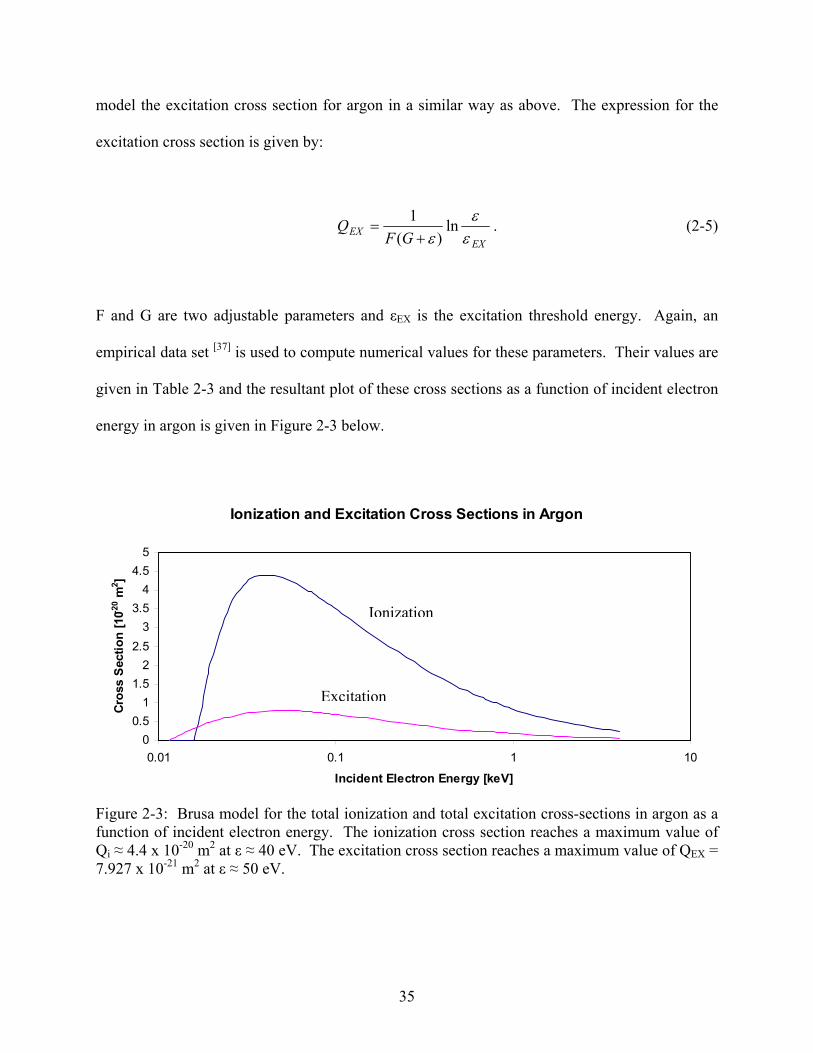
35
model the excitation cross section for argon in a similar way as above. The expression for the
excitation cross section is given by:
EX
EXGF
Qεε
εln
)(
1
+= . (2-5)
F and G are two adjustable parameters and εEX is the excitation threshold energy. Again, an
empirical data set [37]
is used to compute numerical values for these parameters. Their values are
given in Table 2-3 and the resultant plot of these cross sections as a function of incident electron
energy in argon is given in Figure 2-3 below.
Ionization and Excitation Cross Sections in Argon
0
0.5
1
1.5
2
2.5
3
3.5
4
4.5
5
0.01 0.1 1 10
Incident Electron Energy [keV]
Cross Section [10-20 m
2]
Figure 2-3: Brusa model for the total ionization and total excitation cross-sections in argon as a
function of incident electron energy. The ionization cross section reaches a maximum value of
Qi ≈ 4.4 x 10⁻²⁰ m
2 at ε ≈ 40 eV. The excitation cross section reaches a maximum value of QEX =
7.927 x 10⁻²¹ m
2 at ε ≈ 50 eV.
Ionization
Excitation
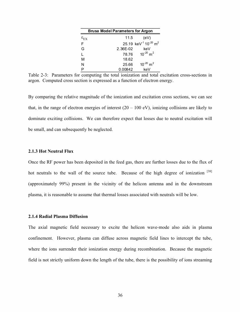
36
εEX 11.5 (eV)
F 25.19 keV-1 10
-20 m
2
G 2.36E-02 keV
L 78.76 10-20 m
2
M 18.62
N 25.66 10-20 m
2
P 0.00842 keV
Brusa Model Parameters for Argon
Table 2-3: Parameters for computing the total ionization and total excitation cross-sections in
argon. Computed cross section is expressed as a function of electron energy.
By comparing the relative magnitude of the ionization and excitation cross sections, we can see
that, in the range of electron energies of interest (20 – 100 eV), ionizing collisions are likely to
dominate exciting collisions. We can therefore expect that losses due to neutral excitation will
be small, and can subsequently be neglected.
2.1.3 Hot Neutral Flux
Once the RF power has been deposited in the feed gas, there are further losses due to the flux of
hot neutrals to the wall of the source tube. Because of the high degree of ionization [38]
(approximately 99%) present in the vicinity of the helicon antenna and in the downstream
plasma, it is reasonable to assume that thermal losses associated with neutrals will be low.
2.1.4 Radial Plasma Diffusion
The axial magnetic field necessary to excite the helicon wave-mode also aids in plasma
confinement. However, plasma can diffuse across magnetic field lines to intercept the tube,
where the ions surrender their ionization energy during recombination. Because the magnetic
field is not strictly uniform down the length of the tube, there is the possibility of ions streaming
37
freely along the field lines until they intercept the walls of the source tube due to curvature in the
field.
2.1.5 Non-Ideal Utilization
Hot neutrals that escape into the plume do not experience electromagnetic body forces and
essentially leave the tube with their thermal speed, in which case, the RF energy used to heat
them is wasted. As discussed previously, the high degree of ionization associated with the
helicon plasma source largely precludes this loss mechanism from playing a major role in the
overall power balance.
2.1.6 RF Irradiance
Some fraction of RF power is lost in non-ideal coupling of RF radiation from the antenna to the
plasma. Transmitted RF will be scattered and dissipated through interactions with the walls of
the vacuum chamber. The operating frequency of 13.56 MHz corresponds to a wavelength of
22.1 meters. Because the non-conducting windows of the vacuum tank are much smaller than
the vacuum electromagnetic wavelength, propagating electromagnetic radiation will remain
effectively shielded inside the tank. In order to measure the losses due to RF irradiance,
measurements must be taken from inside the vacuum chamber.
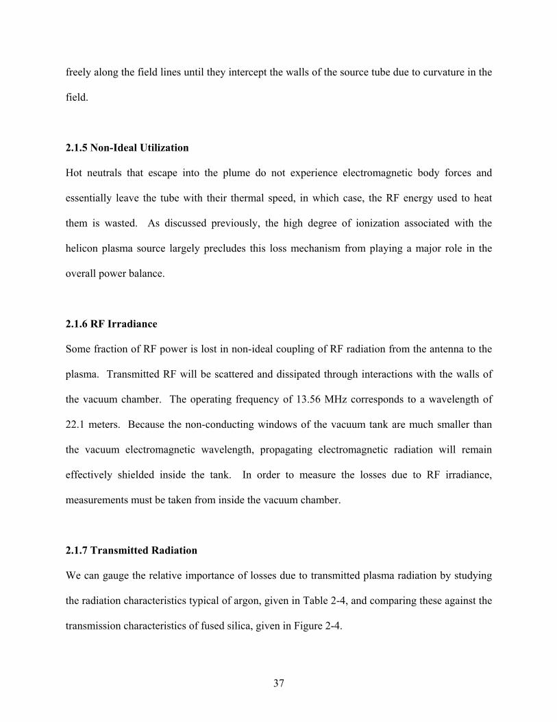
2.1.7 Transmitted Radiation
We can gauge the relative importance of losses due to transmitted plasma radiation by studying
the radiation characteristics typical of argon, given in Table 2-4, and comparing these against the
transmission characteristics of fused silica, given in Figure 2-4.
38
Intensity Wavelength (nm) Spectrum
150 66.186900 Ar II
300 67.094550 Ar II1000 67.185130 Ar II
1000 72.336060 Ar II
180 86.679997 Ar I
150 86.975411 Ar I
180 87.605767 Ar I
180 87.994656 Ar I
150 89.431013 Ar I
300 91.978100 Ar II300 93.205370 Ar II
1000 104.821987 Ar I
500 106.665980 Ar I
Persistent Strong Argon Spectral Lines
Table 2-4: Vacuum wavelength of high-intensity persistent argon spectral lines. Wavelengths
are uniformly below the transparency cutoff for quartz and will therefore contribute to
confinement tube heating [39-41]
.
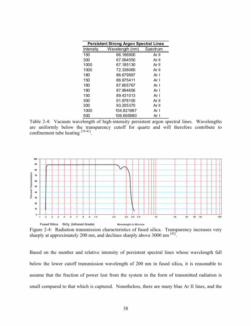
Figure 2-4: Radiation transmission characteristics of fused silica. Transparency increases very
sharply at approximately 200 nm, and declines sharply above 3000 nm [42]
.
Based on the number and relative intensity of persistent spectral lines whose wavelength fall
below the lower cutoff transmission wavelength of 200 nm in fused silica, it is reasonable to
assume that the fraction of power lost from the system in the form of transmitted radiation is
small compared to that which is captured. Nonetheless, there are many blue Ar II lines, and the
39
radiative contribution by these will contribute to the power balance of the system. In the absence
of experimental data, however, these losses are not quantified in this analysis. Future work on
this problem might characterize these losses rigorously using bolometry.
2.1.8 Plume Power
The plume power associated with any rocket device can be expressed most simply as the jet
kinetic power:
2
2
1cmPPLUME &= . (2-6)
Here m& is the mass flow rate in kg/s, c is the exhaust velocity and PPLUME is given in Watts.
Unfortunately, the exhaust velocity associated with the helicon thruster is non-uniform and the
plume is slightly divergent. We know that the thrust is the product of mass flow rate and exit
velocity. We can recast the plume power in terms of the thrust:
m
FPPLUME
&2
2
= . (2-7)
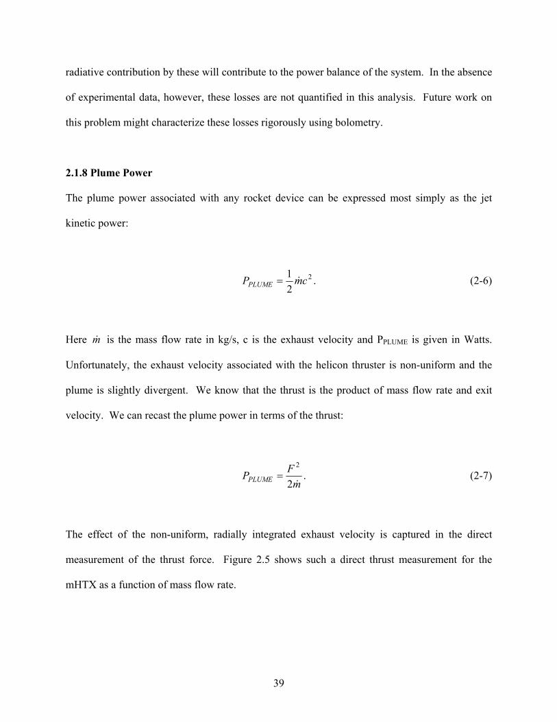
The effect of the non-uniform, radially integrated exhaust velocity is captured in the direct
measurement of the thrust force. Figure 2.5 shows such a direct thrust measurement for the
mHTX as a function of mass flow rate.
40
Figure 2-5: Thrust versus mass flow rate measurement for PRF = 635W, B0 = 1540G as a
function of mass flow rates of argon. This Figure adapted from Reference 31.
Using existing data we can compute an approximate power output in the plume. The standard
volumetric flow rate of 20 sccm used in this study corresponds to a mass flow rate of
approximately 0.55 mg/s.
2.2 Macroscopic Effects
2.2.1 Transmission Hardware Heating
In order to estimate the ohmic losses associated with the transmission hardware, especially the
RF feed through into the vacuum tank, we can measure the heating rate of the vacuum feed
through and from this determine the amount of power lost to ohmic heating.
2.2.2 Confinement Tube Heating
Several of the microscopic heating mechanisms discussed in the previous section contribute to
the effect of heating the walls of the neutral confinement tube. Specifically, plasma diffusion,
radiation by plasma in wavelengths absorbed by fused silica, and the diffusion of hot neutrals all
41
result in confinement tube heating. Derivation of heat flux based on temperature evolution on
the outer wall of the confinement tube will be discussed in the following chapter.
2.2.3 Plume Power
Plume output power measurements can be obtained from previous research [31]
, as described in
Section 2.1.8 and given in Figure 2-5. In this study the plume power is particular to the
operating conditions of the experiment. Without scaling laws describing the variation of plume
power with input power, these results cannot be directly generalized to other experimental
conditions. In particular no information about the input power variation of efficiency can be
extracted.
2.2.4 RF Flux Measurements
Uncoupled electromagnetic radiation which leaves the system can be measured directly using an
RF Flux meter. For this analysis, RF flux will be assumed to be isotropic, based on the reflective
nature of the vacuum chamber walls, so that the total radiated power is given by
∫=S
RFRF dsPOUT
φ . (2-8)
2.3 Power Balance
Using the measured variables discussed in Section 2.2 above, we can define the power balance in
terms of measureable variables as follows:
42
0=−−−−−OUTIN RFPLUMETUBEIONTRANSRF PPPPPP . (2-9)
In the expression above, INRFP is the RF power input to the system from the power supply,
TRANSP the power dissipated in transmission hardware, IONP the power required to ionize the
propellant gas, TUBEP the power lost to the walls of the neutral confinement tube, PLUMEP the
plume power computed directly from thrust measurements, and OUTRFP the uncoupled
electromagnetic radiation that is reflected and dissipated along the walls of the vacuum chamber.
As discussed previously, contributions due to neutral excitation, transmitted radiation, and non-
ideal utilization are expected to be small. These effects will be neglected in the analysis of the
sections that follow.
Having defined the power balance of the system we can now characterize the efficiency.
This is the ratio of the useful power output of the system, in this case the plume power, to the
total input power:
INRF
PLUME
P
P=η . (2-10)
By performing a global characterization of the loss mechanisms in the system, this work will
establish a path toward reducing losses and improving overall system efficiency.
43
Chapter 3
Benchmarking
A methodology and apparatus for obtaining heat flux data from temperature data is outlined in
the sections that follow. Numerical simulation of the confinement tube thermal response is
performed and compared against experimental data to validate the approximated governing
equation for heating rate. A baseline experiment using this approach is discussed. Results of
this baseline experiment are presented. The baseline experiment indicates that measurements
taken at low temperatures can be used to determine incident heat flux to 10% accuracy.
3.1 Analytic Approach
The thermal response of the neutral confinement tube to heat input at the inner boundary is
governed by the heat equation. For a temperature-invariant thermal conductivity, we can express
the heat equation in cylindrical coordinates:
∂
∂+
∂
∂+
∂∂
∂∂
=∂∂
2
2
2
2
2
11
z
TT
rr
Tr
rrk
t
Tc p
θρ . (3-1)
44
The governing equation is subject to boundary constraints on the inner and outer surfaces of the
neutral confinement tube:
≡=
=∇−≡=4
0 )(
)(
o
ri
TRrq
TkRrq
ασ
φ. (3-2)
We can use some relevant insights to reduce the dimension of the problem. First, we assume that
the thermal deposition on the inner boundary is azimuthally symmetric, so that the temperature T
has no angular dependence.
Axial gradients in temperature are driven by the axial gradient of radial heat flux. Radial
temperature gradients, on the other hand, are driven by the local heat flux, according to Fourier’s
law of conduction. Thus, for a scalar conductivity, the ratio of the axial-to-radial temperature
gradients varies in the following way:
)(
)(
z
z
T
T
r
rz
r
z
φφ∇
∝∇
∇. (3-3)
If we assume that the local radial heat flux is much greater than the axial variation, then it is clear
that the effects due to axial gradients in temperature can be neglected. This is borne out
experimentally, as typical axial gradients, 40≅∇ Tz K/cm, compared to typical radial gradients,
200≅∇ Tr K/cm.
45
Finally, because the thickness of the neutral confinement tube is small compared to the
outer radius, 13.00
≅R
d , we can neglect radial effects, including the effect of the radial
geometry on the steady-state thermal gradient. Approximating the tube as a flat surface, the
steady state distribution becomes linear and can be written:
k
z
x
T r )(φ=
∆∆
. (3-4)
Substituting the thermal conductivities for quartz given in Table 1-4, as well as the relevant
dimensions for the neutral confinement tube and the range of heat fluxes of interest (1 W/cm2 ≤
)(zrφ ≤ 3 W/cm2), we obtain a the resultant temperature drop (10.9 K ≤ ∆T ≤ 32.6 K). Even
when compared only to standard temperature, this gradient is negligibly small.
Using these simplifications, we can now integrate the heat equation between the inner
and outer radius of the neutral confinement tube to obtain the ordinary differential equation:
4)()()()( TRrRrdrTkdt
dTdcRR
dt
dTc rOI
R
R
pIOp
I
O
ασφφφρρ −==−==∇−==− ∫ . (3-5)
In the steady state, it is clear that the input heat flux, rφ , is balanced by the radiated power:
4EQr Tασφ = . (3-6)
46
The parameter α is the gray-body parameter. For real processes this parameter takes a value α <
1. This parameter captures the non-ideal nature of the radiative heat transfer, and has the effect
of driving up the required equilibration temperature. For the heat flux ranges of interest, we can
compute a conservative equilibration temperature by assuming the neutral confinement tube
radiates as a blackbody. The heating range 1 W/cm2 ≤ )(zrφ ≤ 3 W/cm
2 corresponds to a final
equilibrium temperature of 648 K ≤ TEQ ≤ 853 K. While TO << TEQ, corresponding roughly to
TO ≤ 0.6TEQ, the radiation term can be neglected, and the heat equation reduces to the simple
form:
)(tdt
dTdc rp φρ = . (3-7)
We can integrate to obtain:
p
rt
r
p dc
tTdss
dcTT
ρ
φφ
ρ
)( )(
10
0
0 +=+= ∫ . (3-8)
This solution is clearly linear in time. In this way, by measuring the slope of the linear portion of
the temperature growth on the outer surface, we can find the associated heat flux, rφ . By
integrating the measured heat flux down the length of the quartz tube, it is then possible to
evaluate the power lost.
In order to assess the validity of the quasi-static, zero-dimensional analysis, described
above, as a means of computing the heat flux to the confinement tube walls, it is helpful to first
obtain a thermal response baseline, wherein the total input power is known. By evaluating the
energy balance using temperature measurements, we can compare the resulting computed power

47
to the known input power. This will yield a measure of the error that we can associate with this
approach.
Figure 3-1: Cutaway of particle confinement tube outfitted with helical resistive element.
Resistor is wound from 22 AWG Nichrome-A stock. Total wound length is 23 cm without
compression. Resistance is RC ≈ 7.4 Ω.
The diagram above illustrates the apparatus for performing the baseline experiment. The source
tube is fitted with a wound resistor in thermal contact with the inner wall of the source tube. The
tube measures 40 cm in length by 2 cm inner diameter. Wall thickness is 1.5 mm.
By simultaneously measuring the temperature of the resistive element and the outer wall
of the confinement tube, we can evaluate the total change in the internal energy of the system
over a given interval of time. This change in energy per unit time is the power we wish to
quantify.

48
Temperature data will be taken with laminated K-type thermocouples on the surfaces of
interest, as shown in Figure 3-2.
Figure 3-2: Thermocouple placement along confinement tube. Five K-type thermocouples are
bonded at equal intervals along the 40 cm length.
49
3.2 Numerical Simulation
We can create a numerical model for the system based on the simplifying assumptions presented
in the previous section. We have assumed that the system can be modeled using Equation 3-5.
We can create a simple finite difference model of this ordinary differential equation to further
test the validity of this assumption. The time-rate-of-change in temperature can be
approximated:
t
TT
dt
dT ii
∆
−≅ +1 . (3-9)
Similarly, the temperature, which is a function of time, can be approximated:
2)( 1 ii TTtT
+≅ + . (3-10)
Using these finite difference approximations, for constant heat flux, rφ , Equation 3-5 can be
written:
4
11
2
+−=
∆
− ++ iir
iiP
TT
t
TTdc ασφρ . (3-11)
The gray-body parameter, α , can be varied to provide the best fit to empirical data. In this way,
numerical modeling of the system can better quantify any deviation from the ideal blackbody
case. There are two methods by which we can simulate the behavior of the system. The first is

50
to factor Equation 3-11 completely and solve the resulting fourth-order polynomial directly for
the roots in δT. The second method involves linearizing Equation 3-11 by assuming that the
temperature increase during each time step is approximately linear. Each of these are discussed
in the sections that follow. Each simulation will be compared against the experimental data
shown in Figures 3-3 and 3-5, using the heat flux derived from the linearized curves in Figures 3-
4 and 3-6.
51
Baseline Temperature Evolution
0
50
100
150
200
250
300
350
0 100 200 300 400 500 600
Time [s]
Temperature [deg C]
Figure 3-3: Temperature growth and saturation for baseline thermal response test. In this
experimental run, temperature is taken from TC2, which is partially occluded by centering clamp
(see Figure C-2 for detailed experimental setup).
Linear Temperature Evolution
y = 1.5158x - 9.3633
0
50
100
150
200
250
300
350
0 20 40 60 80 100 120 140 160 180 200
Time [s]
Temperature [deg C]
Figure 3-4: Linearized temperature growth for baseline thermal response test. The heating rate
of 1.5158 K/s corresponds to a thermal energy flux of 0.3460 W/cm2.
52
Figure 3-5: Temperature growth saturation and decay for 20 sccm Ar, B = 0.165 T, PRF = 1kw.
In this experimental run, tube lip is placed +6 cm forward of plume-side magnet face. Data are
for +4.5 cm forward of plume-side magnet face. No appreciable occlusion is present in this
configuration.
Figure 3-6: Linearized temperature growth for 20 sccm Ar, B = 0.165 T, PRF = 1kw. The
heating rate of 1.6479 K/s corresponds to a thermal energy flux of 0.376 W/cm2.
We will see that modeling of temperature decay properties, as given in Figure 3-5, is
complicated somewhat by the presence of axial gradients due to uneven cooling in the tube.
Heating Rate at +4.5 cm
y = 1.6479x + 0.6655
0
50
100
150
200
250
300
350
400
0 20 40 60 80 100 120
Time [s]
Temperature [deg C]
Temperature Growth-Decay at +4.5 cm
0
50
100
150
200
250
300
0 100 200 300 400 500 600
Time [s]
Temperature [deg C]

53
MATLAB code for both the exact and linearized methods are given in Appendix B.

54
3.2.1 Exact Solution
Expanding Equation 3-11 yields a fourth order polynomial in Ti+1. Carrying out the expansion,
Equation 3-11 can be expressed:
0161616
4644
132
123
14
1 =
∆−+−+
∆++++ ++++ i
pi
ri
piiiiii T
t
dcTT
t
dcTTTTTT
ασ
ρ
ασφ
ασ
ρ. (3-12)
The solution for Ti+1 is the contained in the roots of this polynomial expression. We require that
the solution for the new temperature must be a positive, real-valued, and that ii TT >+1 for
0>rφ . A quartic polynomial with real coefficients, as in this case, may have four real roots,
two real roots and one pair of complex roots, or two pairs of complex roots.
By implementing this expression in MATLAB, we can compare the simulated result with
experimental data. This method consistently returns two real-valued roots, one positive and one
negative, and two complex roots forming a conjugate pair. Valid temperature data is thus limited
to only one root.
The simulated baseline and growth-decay curves computed using this method are
presented in Figures 3-7 and 3-8.
55
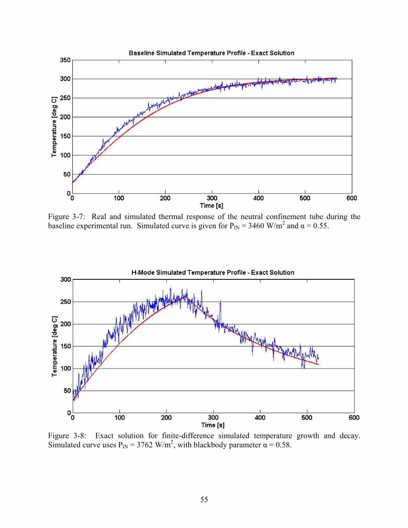
Figure 3-7: Real and simulated thermal response of the neutral confinement tube during the
baseline experimental run. Simulated curve is given for PIN = 3460 W/m2 and α = 0.55.
Figure 3-8: Exact solution for finite-difference simulated temperature growth and decay.
Simulated curve uses PIN = 3762 W/m2, with blackbody parameter α = 0.58.
56
3.2.2 Linearization
As an alternative to iteratively computing the solution for updated temperature directly as in
Section 3.2.1 above, we can also use linearization of Equation 3-11 to obtain an approximate
temperature increment per time-step. We assume that the updated temperature value is
incrementally greater than the previous value, so that:
TTT ii δ+=+1 . (3-13)
We require that the time-step, ∆t, be sufficiently small that 1<<iTTδ . Plugging into Equation
3-11, and discarding all higher order terms in δT, we obtain:
( )TTTt
Tdc rp δ
ασφ
δρ 34 3216
16+−=
∆. (3-14)
We can solve Equation 3-14 for the temperature increment:
3
4
2 tTdc
tTtT
p
r
∆+
∆−∆=
ασρ
ασφδ . (3-15)
This expression gives a simple means of updating temperature at each time step to
approximate the thermal response of the system. Implementing this expression into MATLAB
we can compare the result to the experimentally obtained growth characteristics. The simulated
baseline and growth-decay curves computed using this method are presented in Figures 3-9 and
3-10.

57
Figure 3-9: Simulation of a baseline thermal response curve using a linearization scheme.
Coverage of the thermocouple area by retaining clamp in this experiment drives down the gray
body parameter. This plot corresponds to PIN = 3460 W/m2, and α = 0.55.
Figure 3-10: Simulated temperature growth and decay using a linearization scheme. Simulated
curve uses PIN = 3762 W/m2, with blackbody parameter α = 0.58.

58
It is clear that both methods under predict experimentally obtained results for the choice of
parameters shown. This deviation reaches a maximum in the time range between 100 – 150
seconds for both simulations. In the case of the baseline simulated temperature profile, for the
choice of gray body parameter and the measured heating rate, maximum deviation is
approximately 10%. For the H-Mode heating data, deviation from the centrally averaged
temperature is somewhat greater, approximately 15%. One potential explanation for this
deviation is the inverse variation in specific heat with increasing temperature, which is not
captured in the model. This would explain the temperature variation in heating rate, while
admitting the same steady state behavior observed both in the model and experimentally.
59
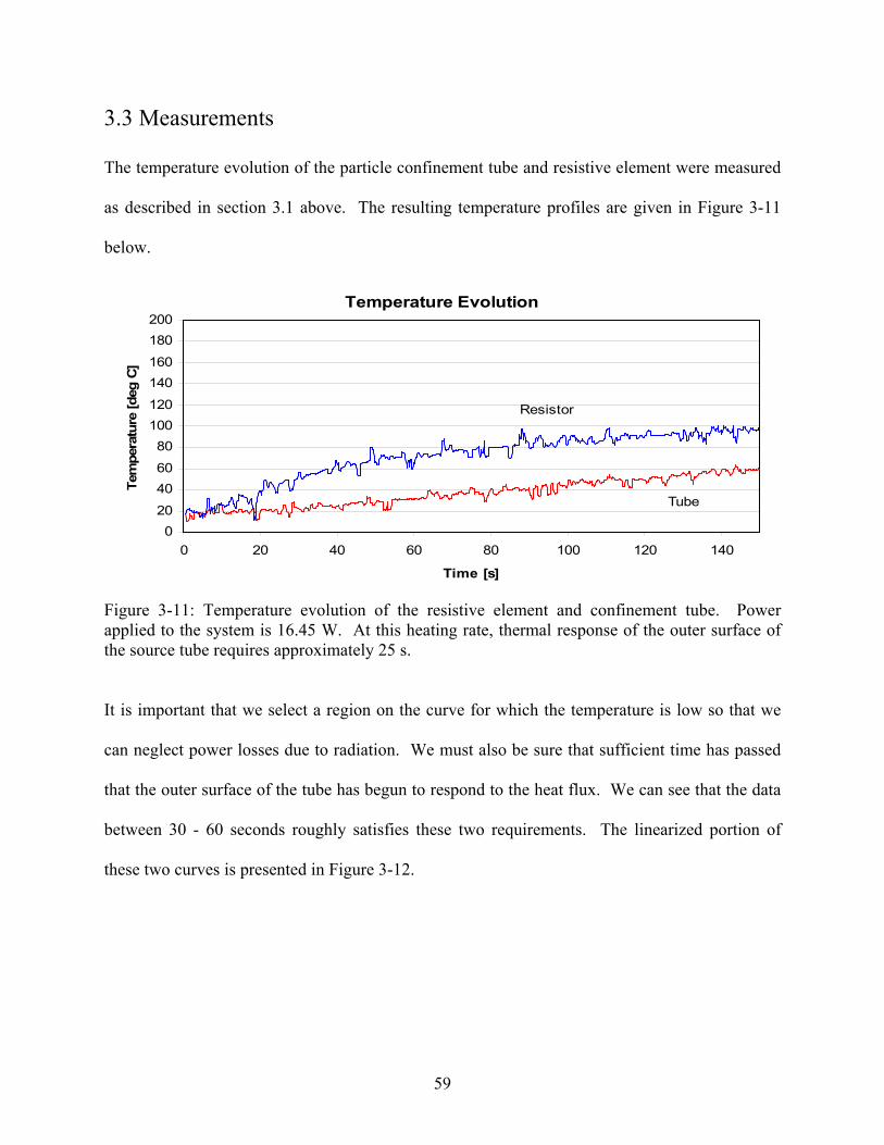
3.3 Measurements
The temperature evolution of the particle confinement tube and resistive element were measured
as described in section 3.1 above. The resulting temperature profiles are given in Figure 3-11
below.
Temperature Evolution
0
20
40
60
80
100
120
140
160
180
200
0 20 40 60 80 100 120 140
Time [s]
Temperature [deg C]
Resistor
Tube
Figure 3-11: Temperature evolution of the resistive element and confinement tube. Power
applied to the system is 16.45 W. At this heating rate, thermal response of the outer surface of
the source tube requires approximately 25 s.
It is important that we select a region on the curve for which the temperature is low so that we
can neglect power losses due to radiation. We must also be sure that sufficient time has passed
that the outer surface of the tube has begun to respond to the heat flux. We can see that the data
between 30 - 60 seconds roughly satisfies these two requirements. The linearized portion of
these two curves is presented in Figure 3-12.
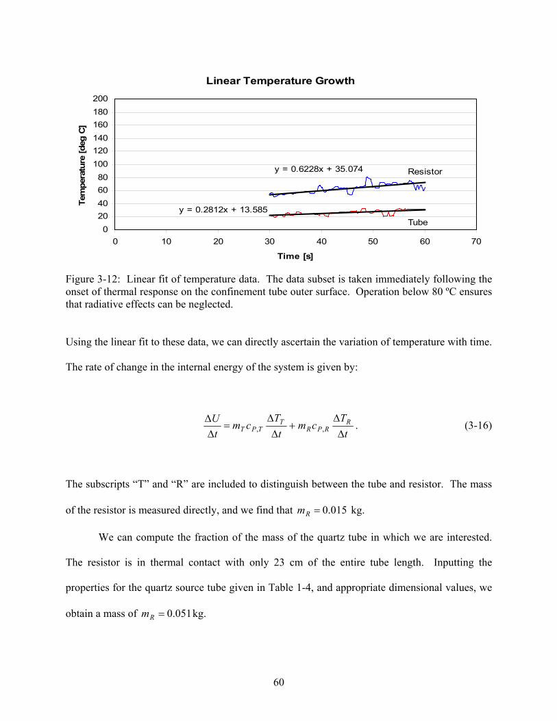
60
Linear Temperature Growth
y = 0.6228x + 35.074
y = 0.2812x + 13.585
0
20
40
60
80
100
120
140
160
180
200
0 10 20 30 40 50 60 70
Time [s]
Temperature [deg C]
Tube
Resistor
Figure 3-12: Linear fit of temperature data. The data subset is taken immediately following the
onset of thermal response on the confinement tube outer surface. Operation below 80 ºC ensures
that radiative effects can be neglected.
Using the linear fit to these data, we can directly ascertain the variation of temperature with time.
The rate of change in the internal energy of the system is given by:
t
Tcm
t
Tcm
t
U RRPR
TTPT ∆
∆+
∆
∆=
∆∆
,, . (3-16)
The subscripts “T” and “R” are included to distinguish between the tube and resistor. The mass
of the resistor is measured directly, and we find that 015.0=Rm kg.
We can compute the fraction of the mass of the quartz tube in which we are interested.
The resistor is in thermal contact with only 23 cm of the entire tube length. Inputting the
properties for the quartz source tube given in Table 1-4, and appropriate dimensional values, we
obtain a mass of 051.0=Rm kg.
61
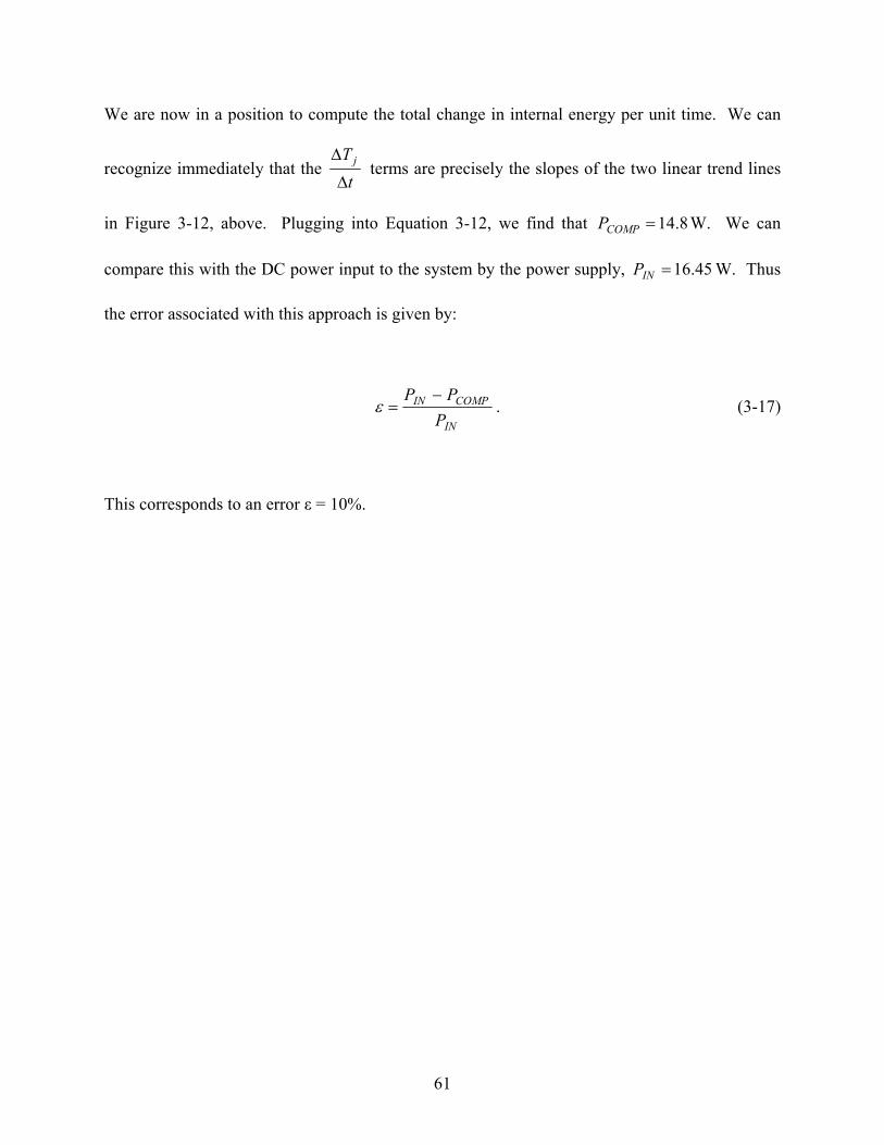
We are now in a position to compute the total change in internal energy per unit time. We can
recognize immediately that the t
T j
∆
∆ terms are precisely the slopes of the two linear trend lines
in Figure 3-12, above. Plugging into Equation 3-12, we find that 8.14=COMPP W. We can
compare this with the DC power input to the system by the power supply, 45.16=INP W. Thus
the error associated with this approach is given by:
IN
COMPIN
P
PP −=ε . (3-17)
This corresponds to an error ε = 10%.
62
Chapter 4
mHTX Power Measurements
Measurement of the heating rate for the RF transmission hardware and neutral confinement tube
is carried out. From these measurements, power losses are derived. Additional losses are
computed for coaxial RF transmission cable, vacuum feed through center conductor, propellant
ionization, and plume power.
4.1 Transmission Hardware Heating
Because of the much higher thermal conductivity of copper compared to fused silica, we can
assume that axial temperature gradients in copper are relatively small and that equilibration times
are short. In considering the losses associated with the transmission hardware as a whole, it is
useful to consider the effects of the coaxial cable, the vacuum feed through, and the antenna
separately, so that the transmission factor in the power balance becomes:
FTANTCOAXTRANS PPPP ++= . (4-1)
63
4.1.1 Coaxial Transmission Cable
As discussed in section 2.1.1, the RF transmission cable that carries the RF signal from the RF
power supply to the impedance matching network is a standard RG-213/U coaxial cable with a
characteristic loss of -4.9 dB/100m. It should be noted that this rating, in which loss is linear in
distance, is only accurate if losses are small. Otherwise, line losses will exhibit logarithmic
behavior. This loss is related to the input-to-output power ratio according to the expression:
=
IN
OUT
P
PG log10 . (4-2)
Converting this to a power ratio, we find that:
−
= 10
049.0
10
L
IN
OUT
P
P. (4-3)
In this expression, L is the length of the cable in meters. The coaxial transmission cable used in
the mHTX has a length of 8 m. Substituting into Equation 4-3, we find that the output power
from the coax is approximately 91.3% of the input power. This means that 8.7% of the input
power is dissipated in the line itself. This loss fraction is sufficiently small that we may take the
linear loss rating associated with the cable as approximately correct. For an input power of 590
W, therefore, we obtain the coaxial transmission loss, PCOAX = 51.33 W.
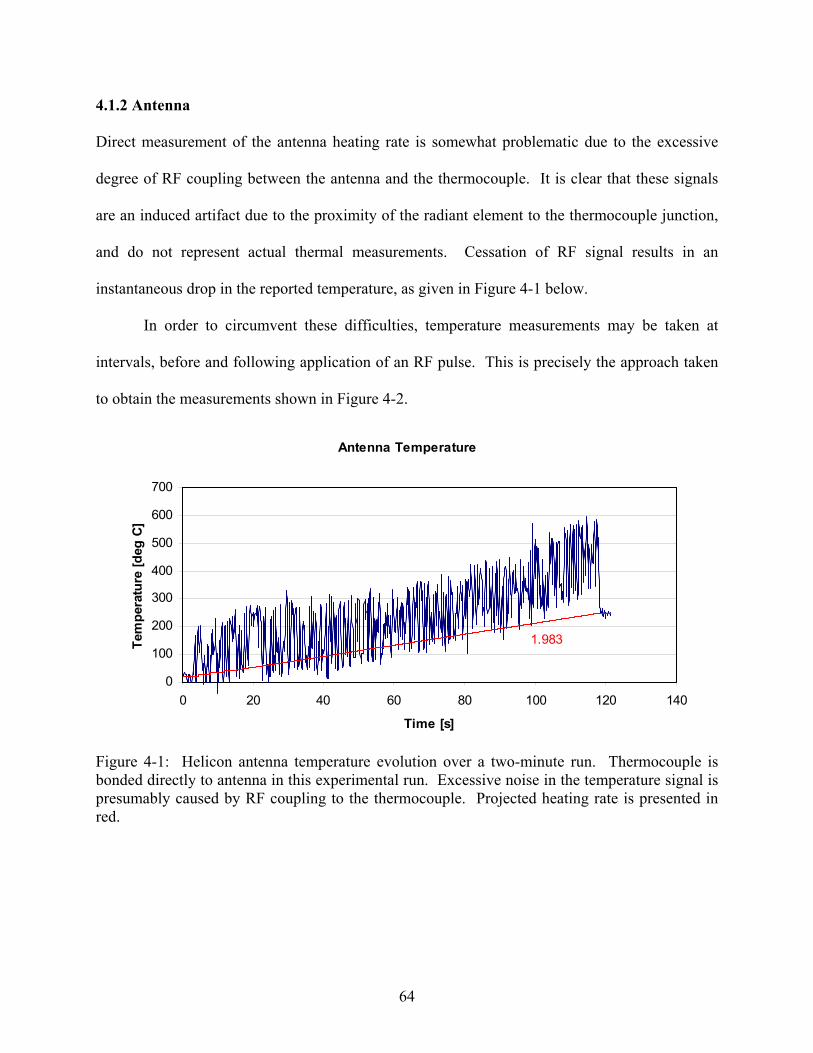
64
4.1.2 Antenna
Direct measurement of the antenna heating rate is somewhat problematic due to the excessive
degree of RF coupling between the antenna and the thermocouple. It is clear that these signals
are an induced artifact due to the proximity of the radiant element to the thermocouple junction,
and do not represent actual thermal measurements. Cessation of RF signal results in an
instantaneous drop in the reported temperature, as given in Figure 4-1 below.
In order to circumvent these difficulties, temperature measurements may be taken at
intervals, before and following application of an RF pulse. This is precisely the approach taken
to obtain the measurements shown in Figure 4-2.
Antenna Temperature
0
100
200
300
400
500
600
700
0 20 40 60 80 100 120 140
Time [s]
Temperature [deg C]
1.983
Figure 4-1: Helicon antenna temperature evolution over a two-minute run. Thermocouple is
bonded directly to antenna in this experimental run. Excessive noise in the temperature signal is
presumably caused by RF coupling to the thermocouple. Projected heating rate is presented in
red.
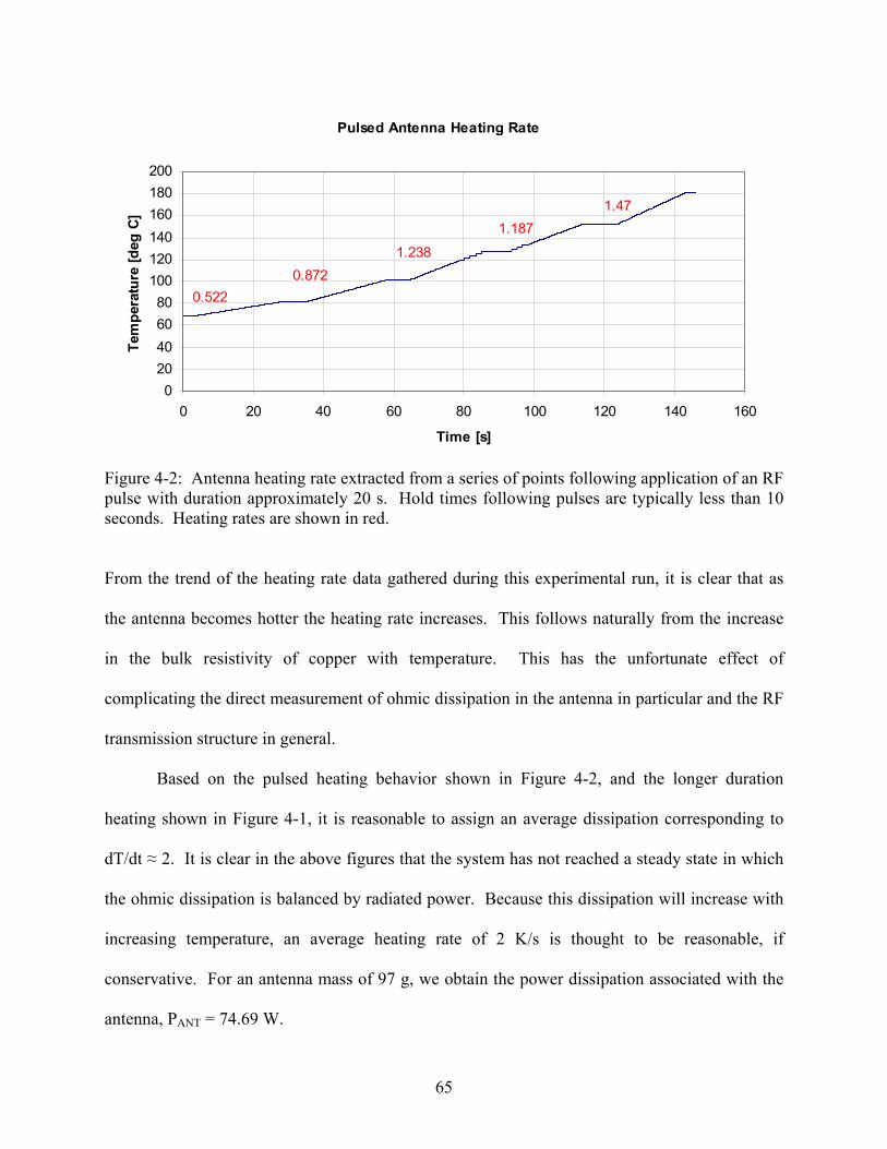
65
Pulsed Antenna Heating Rate
0
20
40
60
80
100
120
140
160
180
200
0 20 40 60 80 100 120 140 160
Time [s]
Temperature [deg C]
0.522
0.872
1.238
1.187
1.47
Figure 4-2: Antenna heating rate extracted from a series of points following application of an RF
pulse with duration approximately 20 s. Hold times following pulses are typically less than 10
seconds. Heating rates are shown in red.
From the trend of the heating rate data gathered during this experimental run, it is clear that as
the antenna becomes hotter the heating rate increases. This follows naturally from the increase
in the bulk resistivity of copper with temperature. This has the unfortunate effect of
complicating the direct measurement of ohmic dissipation in the antenna in particular and the RF
transmission structure in general.
Based on the pulsed heating behavior shown in Figure 4-2, and the longer duration
heating shown in Figure 4-1, it is reasonable to assign an average dissipation corresponding to
dT/dt ≈ 2. It is clear in the above figures that the system has not reached a steady state in which
the ohmic dissipation is balanced by radiated power. Because this dissipation will increase with
increasing temperature, an average heating rate of 2 K/s is thought to be reasonable, if
conservative. For an antenna mass of 97 g, we obtain the power dissipation associated with the
antenna, PANT = 74.69 W.
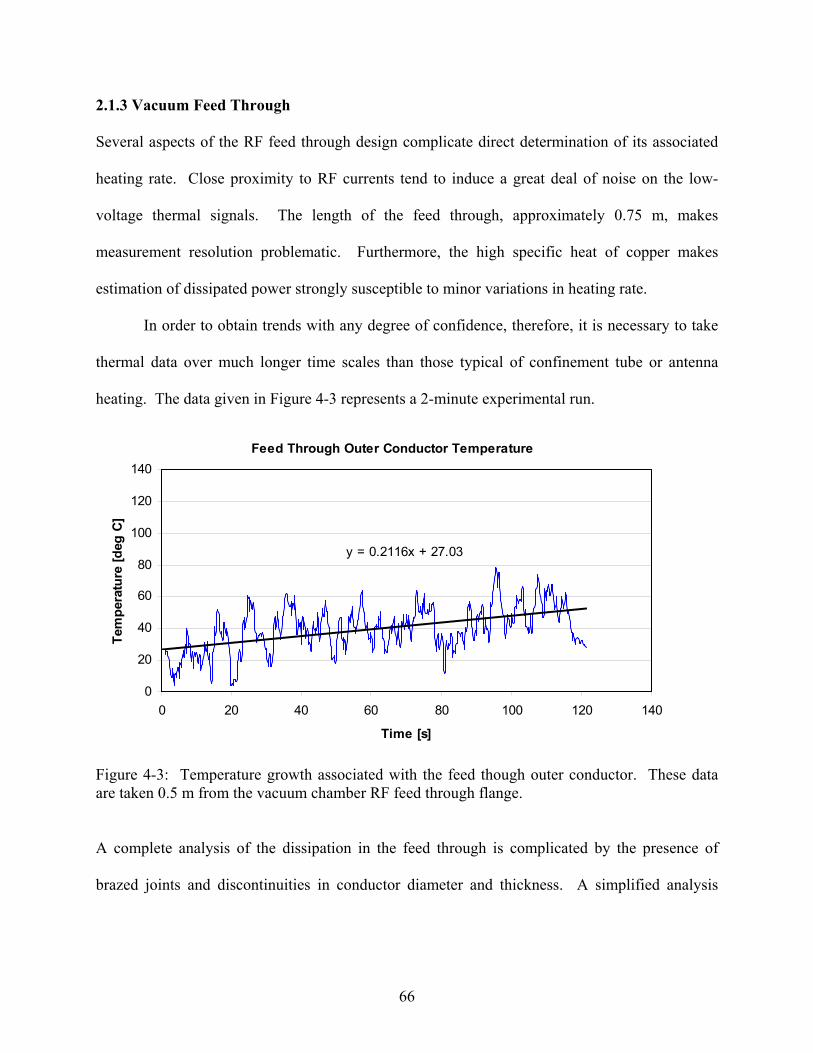
66
2.1.3 Vacuum Feed Through
Several aspects of the RF feed through design complicate direct determination of its associated
heating rate. Close proximity to RF currents tend to induce a great deal of noise on the low-
voltage thermal signals. The length of the feed through, approximately 0.75 m, makes
measurement resolution problematic. Furthermore, the high specific heat of copper makes
estimation of dissipated power strongly susceptible to minor variations in heating rate.
In order to obtain trends with any degree of confidence, therefore, it is necessary to take
thermal data over much longer time scales than those typical of confinement tube or antenna
heating. The data given in Figure 4-3 represents a 2-minute experimental run.
Feed Through Outer Conductor Temperature
y = 0.2116x + 27.03
0
20
40
60
80
100
120
140
0 20 40 60 80 100 120 140
Time [s]
Temperature [deg C]
Figure 4-3: Temperature growth associated with the feed though outer conductor. These data
are taken 0.5 m from the vacuum chamber RF feed through flange.
A complete analysis of the dissipation in the feed through is complicated by the presence of
brazed joints and discontinuities in conductor diameter and thickness. A simplified analysis
67
follows, in which the feed through is assumed to be comprised of two elements, an inner
conductor ¼ in. in diameter and an outer conductor ¾ in. in diameter.
We assume that the thermal conductivity of copper is sufficiently high and dissipative
effects sufficiently uniform that temperature gradients along the feed through may be neglected.
Using a feed through length of 0.75 m and a linear mass of 0.955 kg/m, we can compute the
power dissipated in the outer conductor based on the measurements given in Figure 4-3, POC =
55.13 W.
In the absence of experimental data for the heating rate of the inner conductor, dissipative
losses can be estimated by considering the difference in resistances of the inner and outer
conductor in conjunction with the known dissipation on the outer conductor. For a skin depth of
δ = 17.7 µm, we can use the data for copper in Table 2-1 to compute the resistance associated
with a copper conductor carrying an RF signal of 13.56 MHz. For a conductor outer diameter of
1.9 cm, we find the resistance is approximately ROC = 0.805 Ω/m. For an outer diameter of 0.64
cm, on the other hand, this resistance becomes RIC = 2.41 Ω/m. Neglecting temperature
variations in conductivity, we can therefore roughly estimate that the dissipative loss on the inner
conductor will be three times that on the outer conductor.
Using this simplified analysis we obtain PFT = 220.52 W.
4.2 Ionization Power
The power consumed in ionizing the propellant gas is proportional to the propellant flow rate and
inversely proportional to the molar mass of the species, as discussed in Section 2.1.2. For argon,
the ionization power requirement is given by PION = 1.13*F, where F is the flow rate in sccm.
For our reference condition of 20 sccm Ar, the power requirement is PION = 22.6 W.
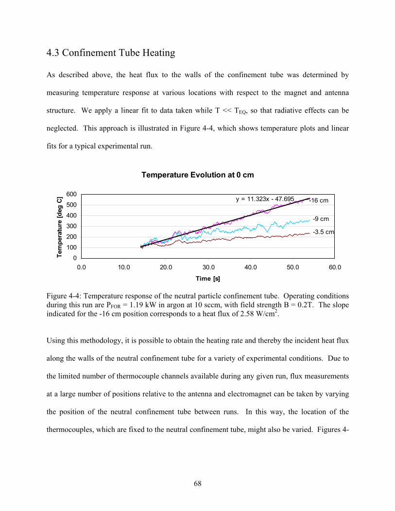
68
4.3 Confinement Tube Heating
As described above, the heat flux to the walls of the confinement tube was determined by
measuring temperature response at various locations with respect to the magnet and antenna
structure. We apply a linear fit to data taken while T << TEQ, so that radiative effects can be
neglected. This approach is illustrated in Figure 4-4, which shows temperature plots and linear
fits for a typical experimental run.
Figure 4-4: Temperature response of the neutral particle confinement tube. Operating conditions
during this run are PFOR = 1.19 kW in argon at 10 sccm, with field strength B = 0.2T. The slope
indicated for the -16 cm position corresponds to a heat flux of 2.58 W/cm2.
Using this methodology, it is possible to obtain the heating rate and thereby the incident heat flux
along the walls of the neutral confinement tube for a variety of experimental conditions. Due to
the limited number of thermocouple channels available during any given run, flux measurements
at a large number of positions relative to the antenna and electromagnet can be taken by varying
the position of the neutral confinement tube between runs. In this way, the location of the
thermocouples, which are fixed to the neutral confinement tube, might also be varied. Figures 4-
Temperature Evolution at 0 cm
y = 11.323x - 47.695
0
100
200
300
400
500
600
0.0 10.0 20.0 30.0 40.0 50.0 60.0
Time [s]
Temperature [deg C]
-16 cm
-9 cm
-3.5 cm

69
5 through 4-8 give the heating rata data which are used to derive the flux profiles given in
Figures 4-9 and 4-10.
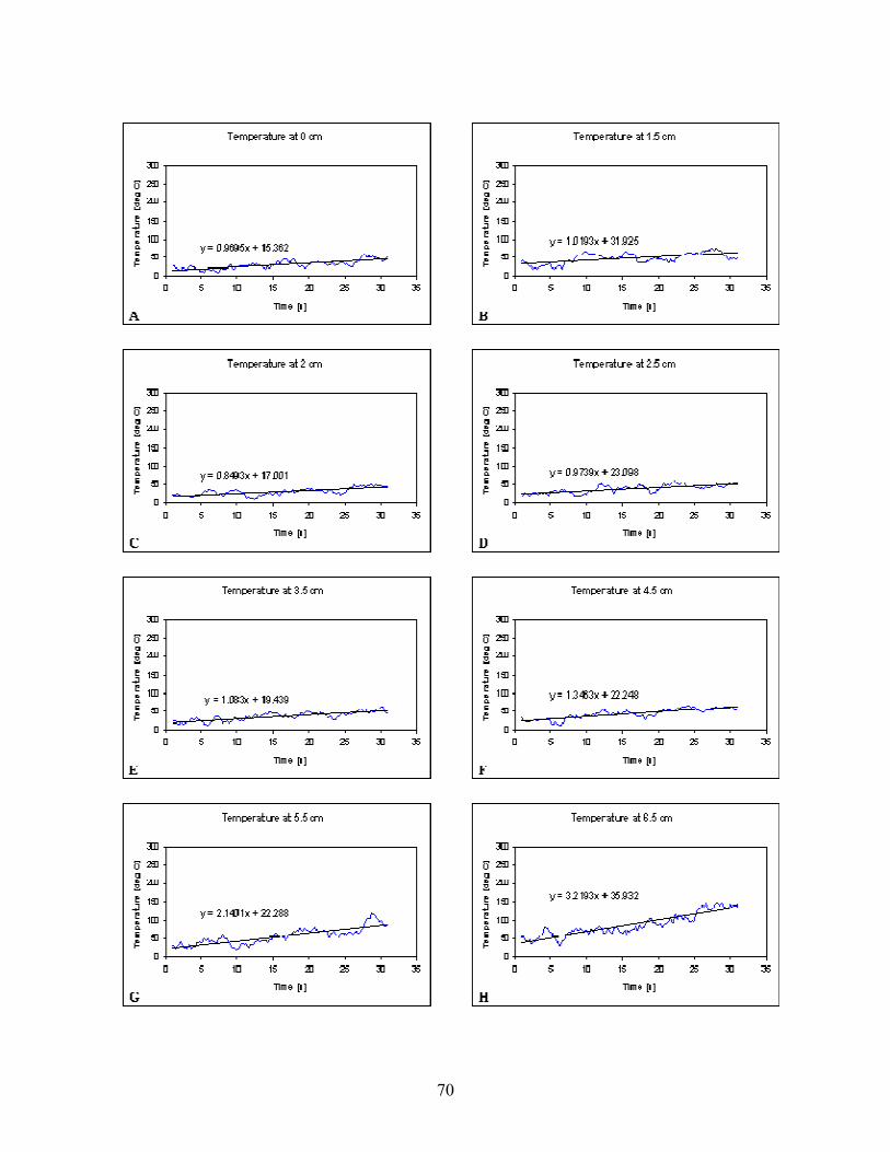
70
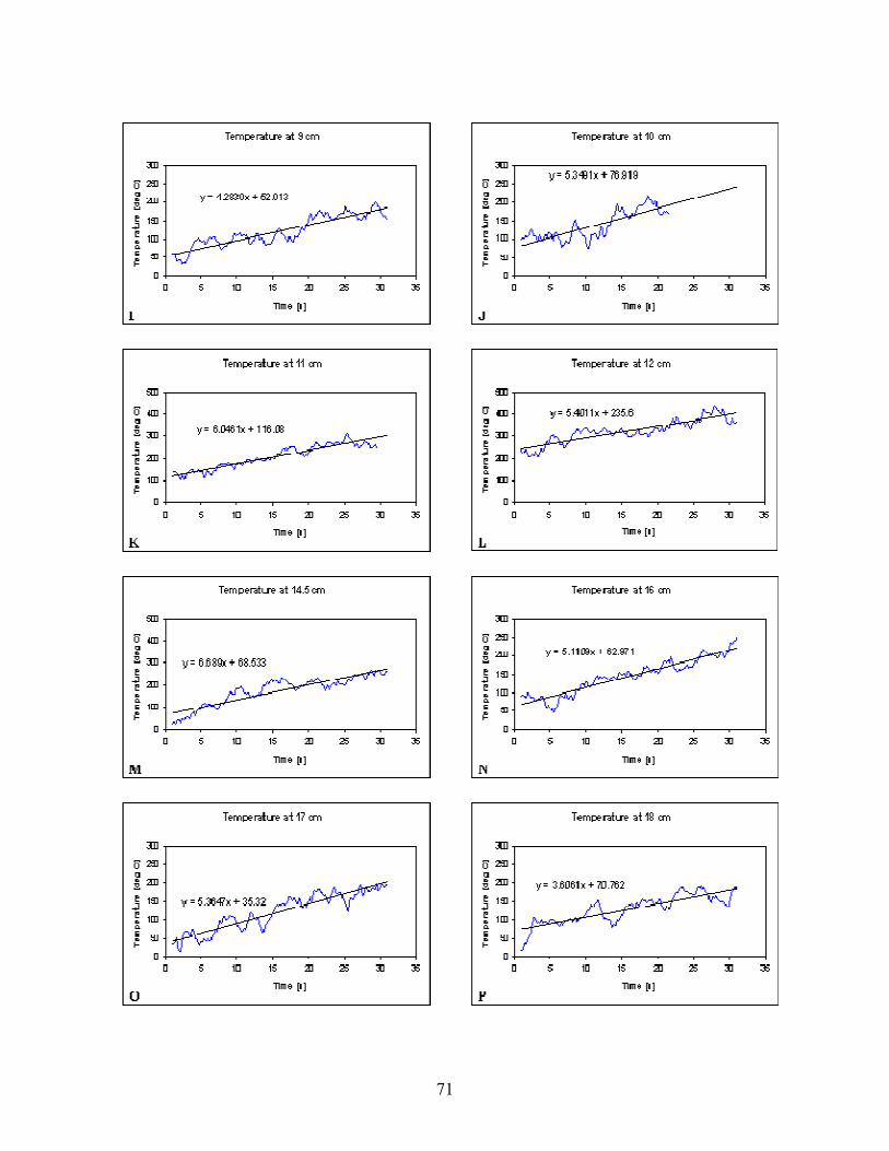
71
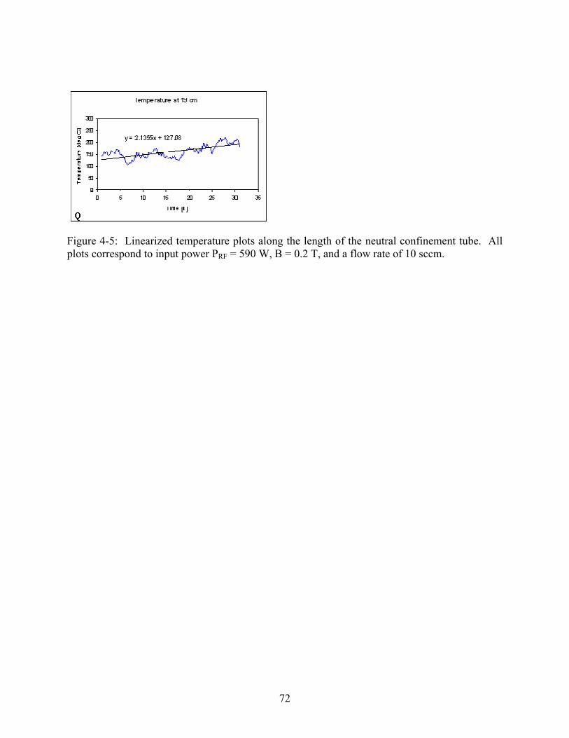
72
Figure 4-5: Linearized temperature plots along the length of the neutral confinement tube. All
plots correspond to input power PRF = 590 W, B = 0.2 T, and a flow rate of 10 sccm.
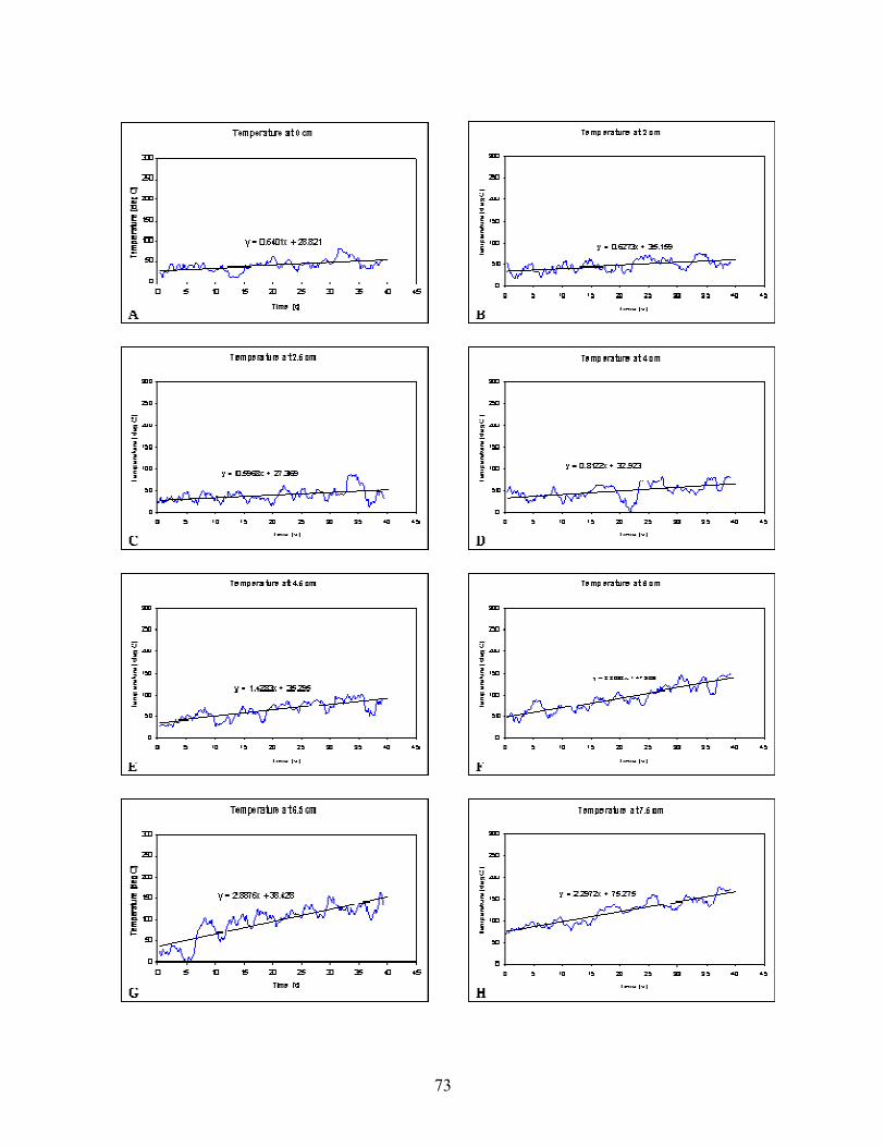
73
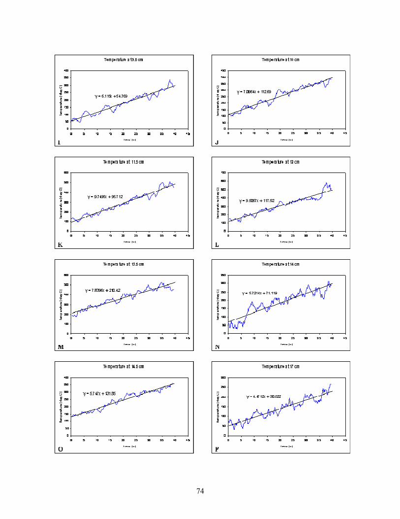
74
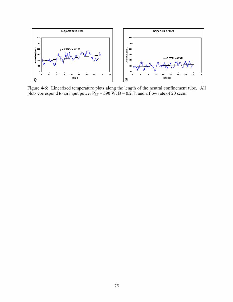
75
Figure 4-6: Linearized temperature plots along the length of the neutral confinement tube. All
plots correspond to an input power PRF = 590 W, B = 0.2 T, and a flow rate of 20 sccm.
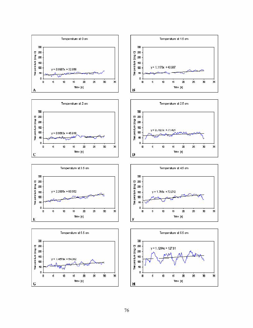
76
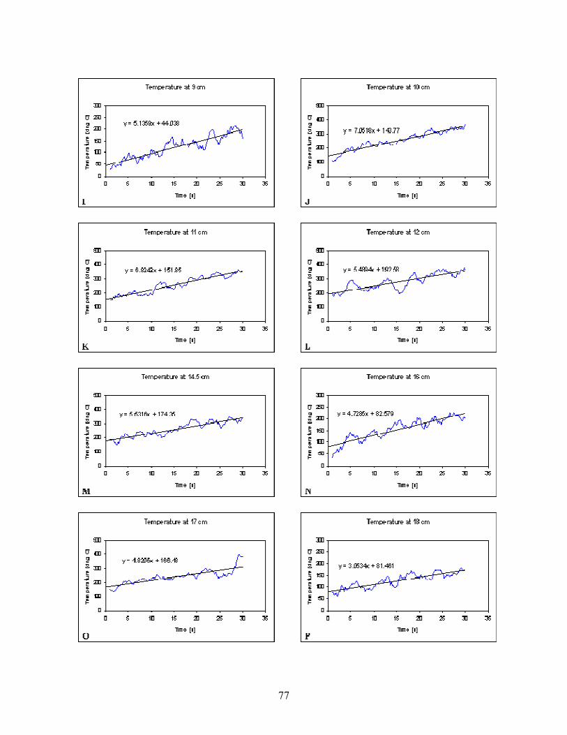
77
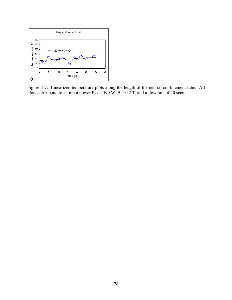
78
Figure 4-7: Linearized temperature plots along the length of the neutral confinement tube. All
plots correspond to an input power PRF = 590 W, B = 0.2 T, and a flow rate of 40 sccm.
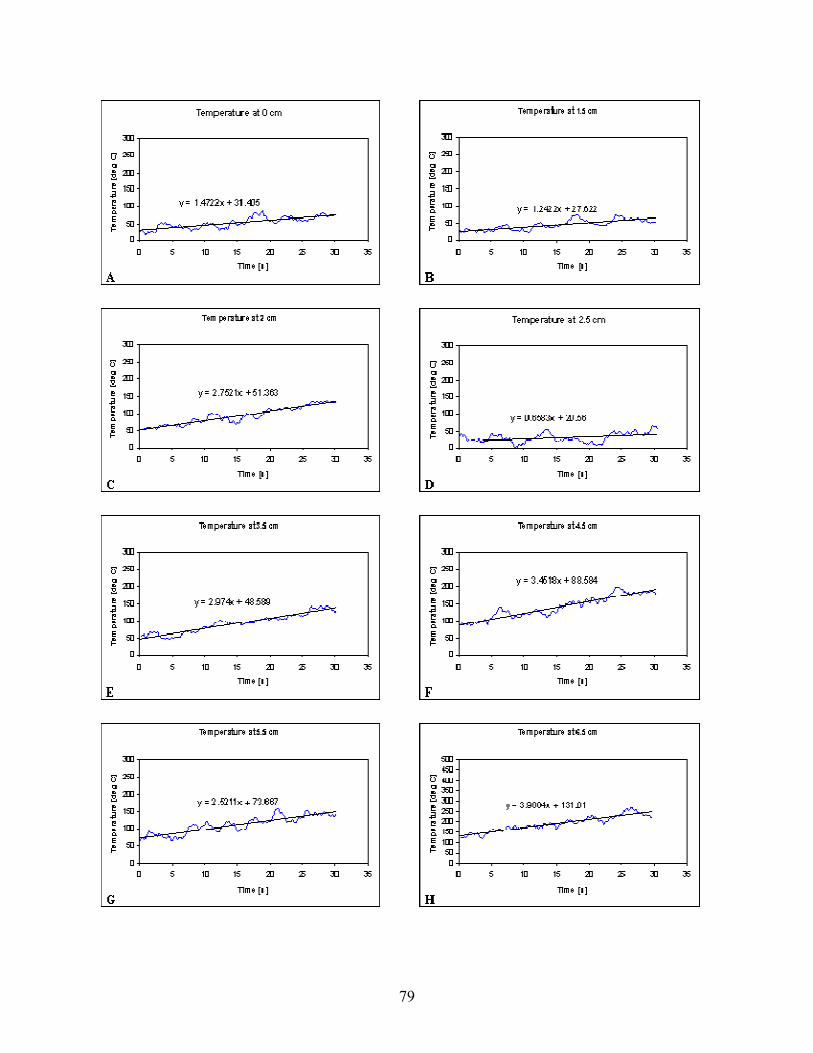
79
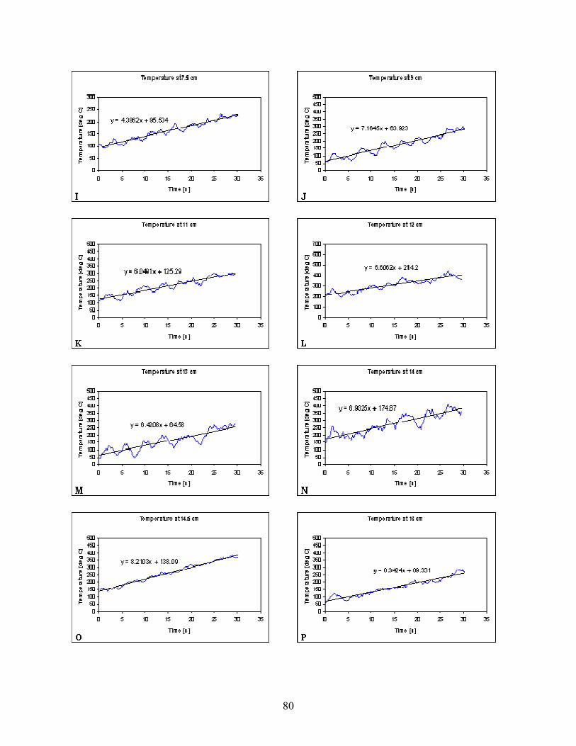
80
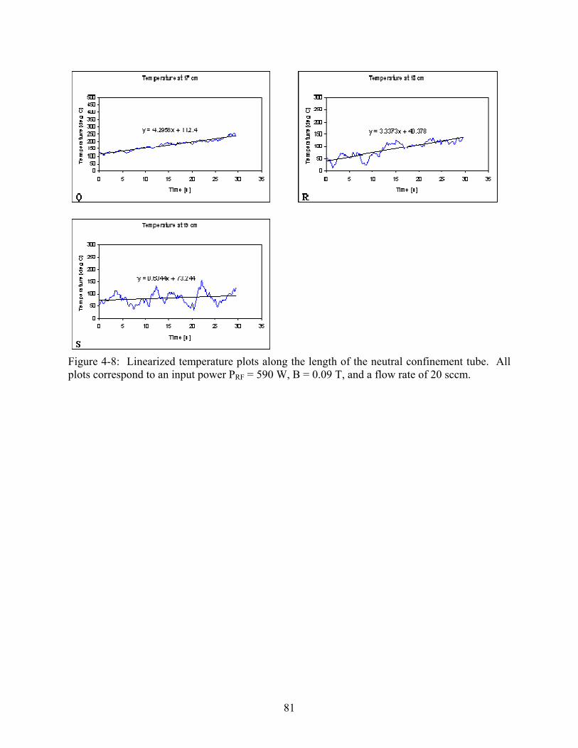
81
Figure 4-8: Linearized temperature plots along the length of the neutral confinement tube. All
plots correspond to an input power PRF = 590 W, B = 0.09 T, and a flow rate of 20 sccm.

82
Using these slopes we can derive the energy flux to the neutral confinement tube using exactly
the method outlined in Sections 3.1 and 3.3. Following this approach, we obtain the curves
given in Figures 4-9 through 4-10 below. In considering these figures it is important to note that
the plume-side electromagnetic face corresponds to x = 0 cm. Propellant is injected upstream at
x = 40 cm, travels in the xe− direction, and is exhausted at x = 0 cm.
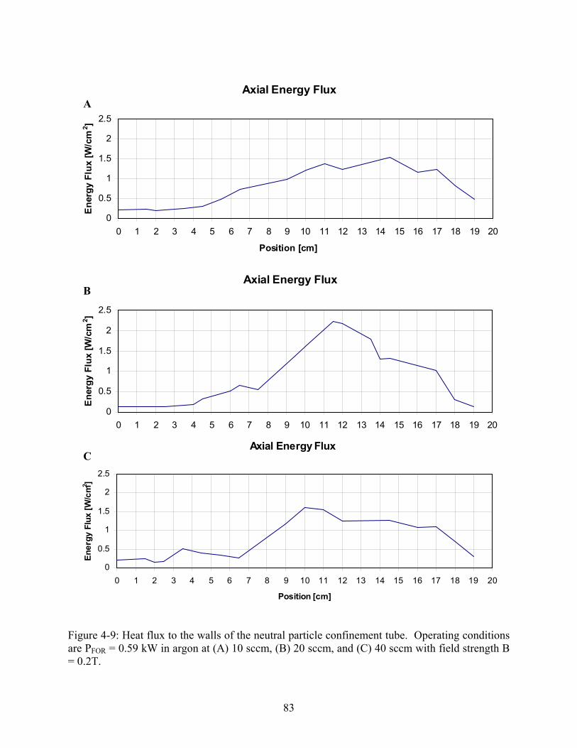
83
Figure 4-9: Heat flux to the walls of the neutral particle confinement tube. Operating conditions
are PFOR = 0.59 kW in argon at (A) 10 sccm, (B) 20 sccm, and (C) 40 sccm with field strength B
= 0.2T.
Axial Energy Flux
0
0.5
1
1.5
2
2.5
0 1 2 3 4 5 6 7 8 9 10 11 12 13 14 15 16 17 18 19 20
Position [cm]
Energy Flux [W/cm
2]
Axial Energy Flux
0
0.5
1
1.5
2
2.5
0 1 2 3 4 5 6 7 8 9 10 11 12 13 14 15 16 17 18 19 20
Position [cm]
Energy Flux [W/cm
2]
Axial Energy Flux
0
0.5
1
1.5
2
2.5
0 1 2 3 4 5 6 7 8 9 10 11 12 13 14 15 16 17 18 19 20
Position [cm]
Energy Flux [W/cm2]
A
B
C
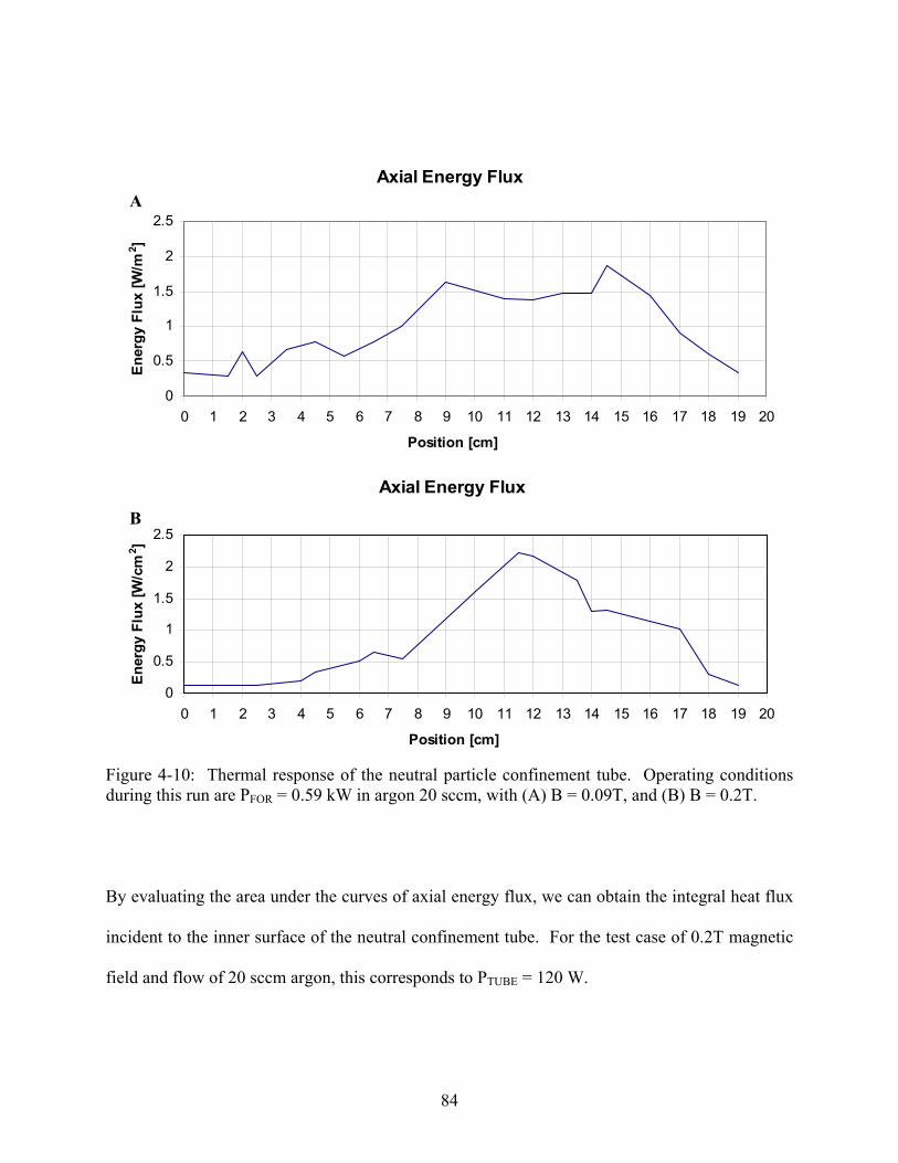
84
Figure 4-10: Thermal response of the neutral particle confinement tube. Operating conditions
during this run are PFOR = 0.59 kW in argon 20 sccm, with (A) B = 0.09T, and (B) B = 0.2T.
By evaluating the area under the curves of axial energy flux, we can obtain the integral heat flux
incident to the inner surface of the neutral confinement tube. For the test case of 0.2T magnetic
field and flow of 20 sccm argon, this corresponds to PTUBE = 120 W.
Axial Energy Flux
0
0.5
1
1.5
2
2.5
0 1 2 3 4 5 6 7 8 9 10 11 12 13 14 15 16 17 18 19 20
Position [cm]
Energy Flux [W/cm
2]
Axial Energy Flux
0
0.5
1
1.5
2
2.5
0 1 2 3 4 5 6 7 8 9 10 11 12 13 14 15 16 17 18 19 20
Position [cm]
Energy Flux [W/m
2]
A
B
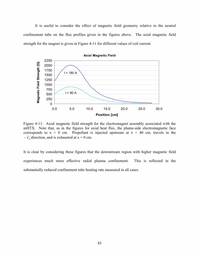
85
It is useful to consider the effect of magnetic field geometry relative to the neutral
confinement tube on the flux profiles given in the figures above. The axial magnetic field
strength for the magnet is given in Figure 4-11 for different values of coil current.
Axial Magnetic Field
0
250
500
750
1000
1250
1500
1750
2000
2250
0.0 5.0 10.0 15.0 20.0 25.0 30.0
Position [cm]
Magnetic Field Strength [G]
I = 180 A
I = 80 A
Figure 4-11: Axial magnetic field strength for the electromagnet assembly associated with the
mHTX. Note that, as in the figures for axial heat flux, the plume-side electromagnetic face
corresponds to x = 0 cm. Propellant is injected upstream at x = 40 cm, travels in the
xe− direction, and is exhausted at x = 0 cm.
It is clear by considering these figures that the downstream region with higher magnetic field
experiences much more effective radial plasma confinement. This is reflected in the
substantially reduced confinement tube heating rate measured in all cases.
86
4.4 Plume Power
Using thrust data taken on the mHTX experiment in a previous study [31]
and provided in Figure
2-5, we can obtain the thrust for the standard flow of 20 sccm of argon, or 0.55 mg/s, used in our
test case. This corresponds to a thrust of approximately 8.5 mN. Plugging into Equation 2-7, we
find the plume power is approximately PPLUME = 65 W.
4.5 RF Flux Measurements
In order to measure the uncoupled RF flux inside the chamber during operation of the thruster,
the RF flux meter was placed inside the chamber. Because the device is not suitable for
operation under vacuum, the helicon antenna was driven under atmospheric conditions to
quantify the power radiated from the antenna. During this analog run, a maximum sustained
forward power of 400 W was achieved, in which an RF flux of approximately 160 µW/cm2 was
obtained. We can obtain an upper bound on the RF deposition along the tank wall by assuming
that the measured RF is isotropic, and all the energy is absorbed by the tank wall. We can model
the vacuum chamber as a perfect cylinder with diameter 1.5 m and length 1.6 m. In this case,
substituting into Equation 2-8 we obtain:
( ) RFRF rrLPOUT
φππ 222 += . (4-4)
Solving with the appropriate values, we obtain 05.18=OUT
RFP W.
87
Chapter 5
Conclusion
In this section the observations from the previous chapter are applied to the power balance,
outlined in Chapter 2. An accounting of all the losses and outputs associated with the system is
completed and the overall system efficiency is computed. Avenues are identified for improving
overall efficiency. Recommendations are offered for future work.
5.1 Power Balance Tabulation
A final accounting of the output and loss mechanisms associated with the mHTX experiment is
included in Table 5-1 below. Of the 590 W of forward power consistently applied across
experimental runs, approximately 572 W have been accounted for. This represents about 97% of
the total power.
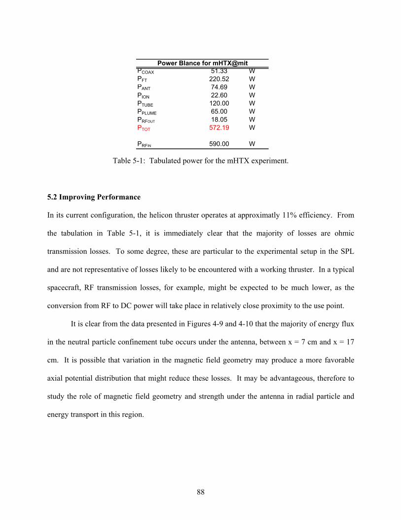
88
Table 5-1: Tabulated power for the mHTX experiment.
5.2 Improving Performance
In its current configuration, the helicon thruster operates at approximatly 11% efficiency. From
the tabulation in Table 5-1, it is immediately clear that the majority of losses are ohmic
transmission losses. To some degree, these are particular to the experimental setup in the SPL
and are not representative of losses likely to be encountered with a working thruster. In a typical
spacecraft, RF transmission losses, for example, might be expected to be much lower, as the
conversion from RF to DC power will take place in relatively close proximity to the use point.
It is clear from the data presented in Figures 4-9 and 4-10 that the majority of energy flux
in the neutral particle confinement tube occurs under the antenna, between x = 7 cm and x = 17
cm. It is possible that variation in the magnetic field geometry may produce a more favorable
axial potential distribution that might reduce these losses. It may be advantageous, therefore to
study the role of magnetic field geometry and strength under the antenna in radial particle and
energy transport in this region.
PCOAX 51.33 W
PFT 220.52 W
PANT 74.69 W
22.60 W
120.00 W
65.00 W
18.05 W
572.19 W
590.00 W
PRFOUTPTOT
PRFIN
Power Blance for mHTX@mit
PIONPTUBEPPLUME
89
5.3 Recommendations for Future Work
Future work on the helicon thruster in general and the power balance in particular should first
focus on reducing losses associated with power transmission hardware. This might be
accomplished in a variety of ways: by reducing operating frequency; increasing conductor
surface area; and reducing the source-to-sink distance associated with the experiment.
Second, there is a need for a more precise measurement of the power dissipated in the RF
feed through. Losses computed from heating rates in this study indicate that power dissipation in
the feed through may consume over one-third of the power applied to the system. Further
studies with more spatial precision should be undertaken to further characterize this loss path.
Additional measurements for losses in the RF impedance matching network will also be
beneficial.
Third, measurements of radiation at transmitted wavelengths should be taken using a
bolometer to quantify this loss.
Finally, concurrently with the previous recommendation, the mHTX experiment should
migrate to the use of permanent magnets for generation of the magnetic field. Several
commercially available options exist for permanent magnets, especially rare earth magnets such
as Neodymium-Iron-Boron (NdFeB), which can provide comparable or greater fields, which
may be more easily manipulated in experiments, for a small fraction of the mass required by
electromagnets.

90
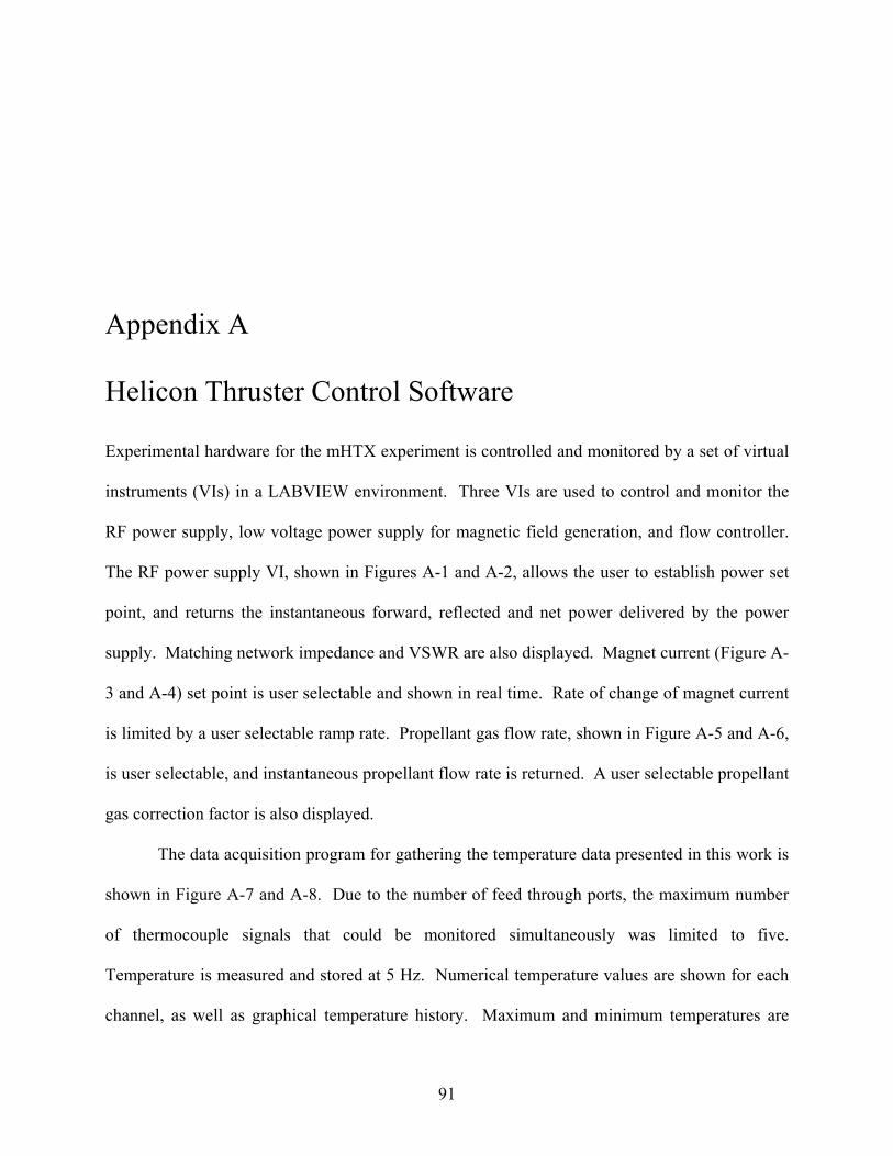
91
Appendix A
Helicon Thruster Control Software
Experimental hardware for the mHTX experiment is controlled and monitored by a set of virtual
instruments (VIs) in a LABVIEW environment. Three VIs are used to control and monitor the
RF power supply, low voltage power supply for magnetic field generation, and flow controller.
The RF power supply VI, shown in Figures A-1 and A-2, allows the user to establish power set
point, and returns the instantaneous forward, reflected and net power delivered by the power
supply. Matching network impedance and VSWR are also displayed. Magnet current (Figure A-
3 and A-4) set point is user selectable and shown in real time. Rate of change of magnet current
is limited by a user selectable ramp rate. Propellant gas flow rate, shown in Figure A-5 and A-6,
is user selectable, and instantaneous propellant flow rate is returned. A user selectable propellant
gas correction factor is also displayed.
The data acquisition program for gathering the temperature data presented in this work is
shown in Figure A-7 and A-8. Due to the number of feed through ports, the maximum number
of thermocouple signals that could be monitored simultaneously was limited to five.
Temperature is measured and stored at 5 Hz. Numerical temperature values are shown for each
channel, as well as graphical temperature history. Maximum and minimum temperatures are

92
user selectable and set the y-axis temperature range. A variety of junction types can be selected,
including K-type used in this study. The temperature of the cold junction is user defined. This is
typically set to the standard temperature, 25˚C.
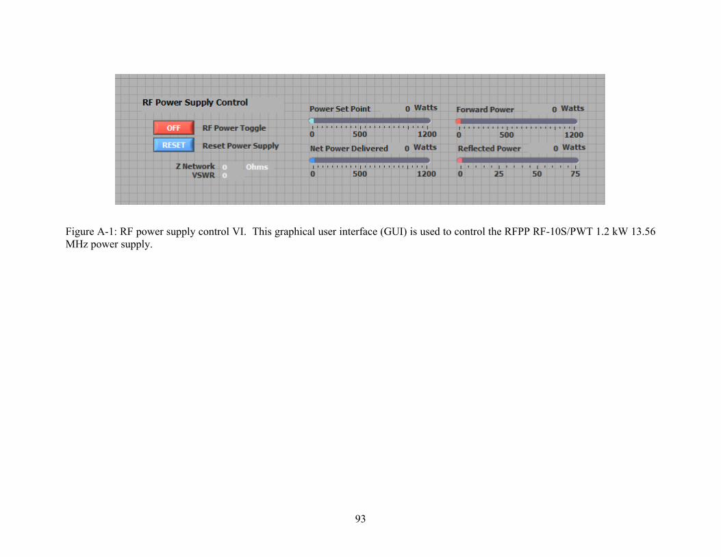
93
Figure A-1: RF power supply control VI. This graphical user interface (GUI) is used to control the RFPP RF-10S/PWT 1.2 kW 13.56
MHz power supply.
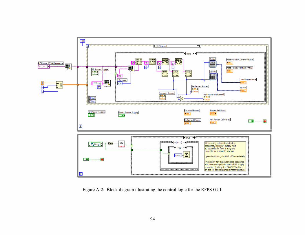
94
Figure A-2: Block diagram illustrating the control logic for the RFPS GUI.
95
Figure A-3: Magnet control VI. This GUI is used to control the Agilent N5761A 6V 180A 1080W power supply supplying the
magnetic field for the mHTX.
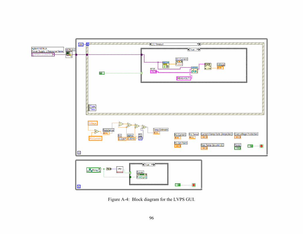
96
Figure A-4: Block diagram for the LVPS GUI.
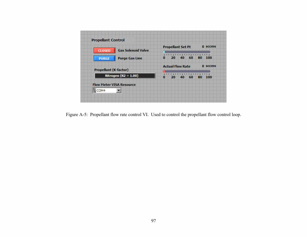
97
Figure A-5: Propellant flow rate control VI. Used to control the propellant flow control loop.
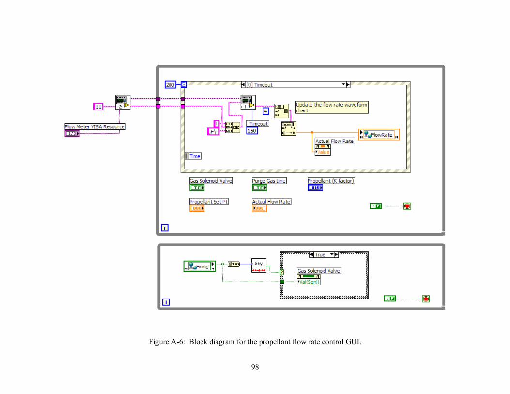
98
Figure A-6: Block diagram for the propellant flow rate control GUI.
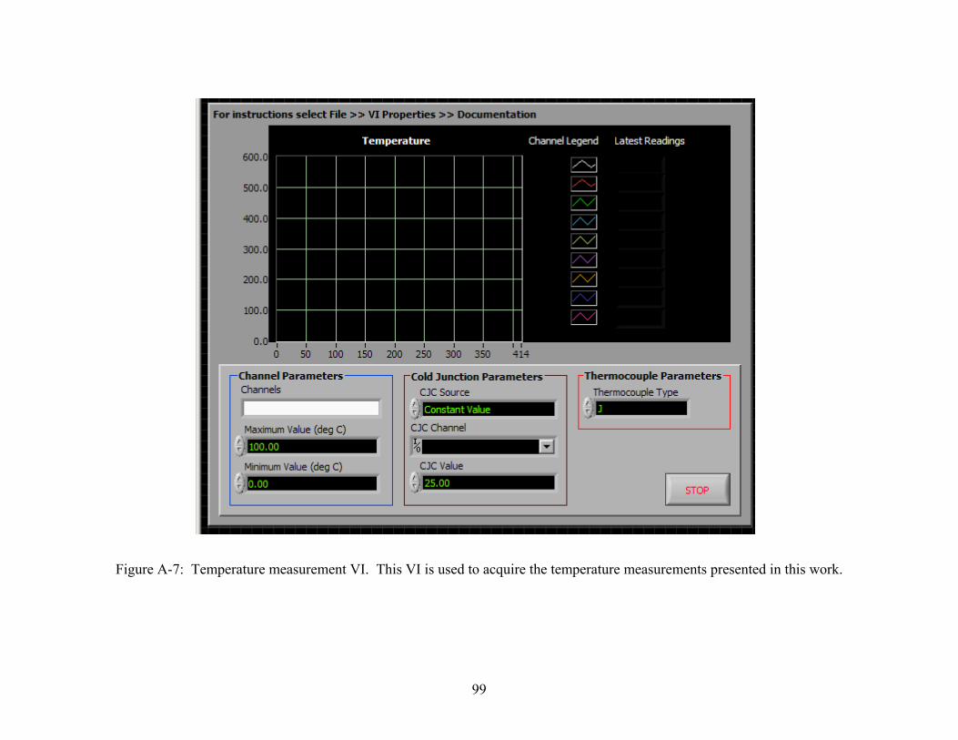
99
Figure A-7: Temperature measurement VI. This VI is used to acquire the temperature measurements presented in this work.
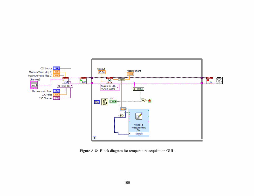
100
Figure A-8: Block diagram for temperature acquisition GUI.

101
Appendix B
Finite Difference Modeling Code
The finite-difference model of the thermal response of the neutral confinement tube to constant
heat flux given in Section 3.2 was completed in MATLAB R2006a. Two methods were used in
solving this model. The first is an exact solution based on evaluating the roots of the fourth-
order finite difference model. The second is a less computationally intensive, approximate
method based on linearization of the temperature response. Code for the MATLAB .m files used
to implement this method are included in the figures that follow.
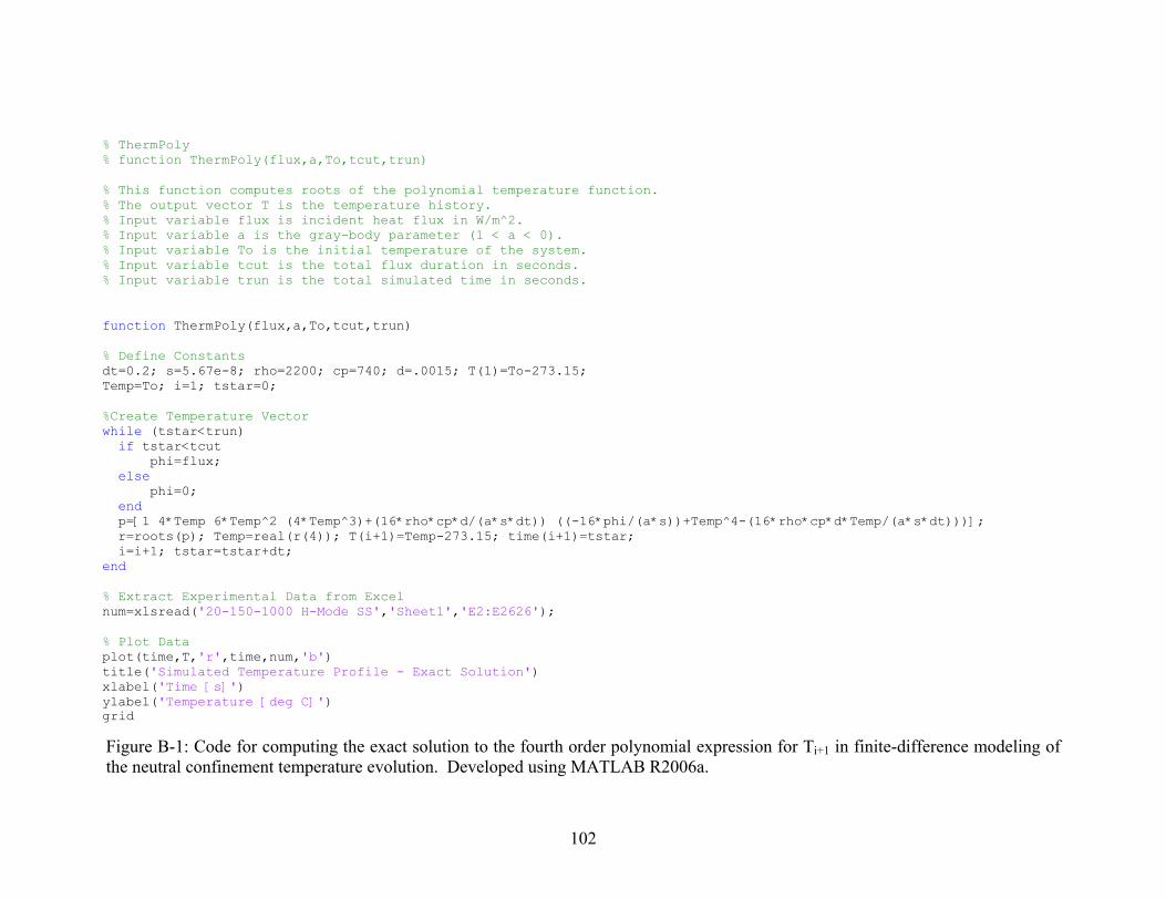
102
Figure B-1: Code for computing the exact solution to the fourth order polynomial expression for Ti+1 in finite-difference modeling of
the neutral confinement temperature evolution. Developed using MATLAB R2006a.
% ThermPoly % function ThermPoly(flux,a,To,tcut,trun)
% This function computes roots of the polynomial temperature function. % The output vector T is the temperature history. % Input variable flux is incident heat flux in W/m^2. % Input variable a is the gray-body parameter (1 < a < 0). % Input variable To is the initial temperature of the system. % Input variable tcut is the total flux duration in seconds. % Input variable trun is the total simulated time in seconds.
function ThermPoly(flux,a,To,tcut,trun)
% Define Constants dt=0.2; s=5.67e-8; rho=2200; cp=740; d=.0015; T(1)=To-273.15; Temp=To; i=1; tstar=0;
%Create Temperature Vector while (tstar<trun) if tstar<tcut phi=flux; else phi=0; end p=[1 4*Temp 6*Temp^2 (4*Temp^3)+(16*rho*cp*d/(a*s*dt)) ((-16*phi/(a*s))+Temp^4-(16*rho*cp*d*Temp/(a*s*dt)))]; r=roots(p); Temp=real(r(4)); T(i+1)=Temp-273.15; time(i+1)=tstar; i=i+1; tstar=tstar+dt; end
% Extract Experimental Data from Excel num=xlsread('20-150-1000 H-Mode SS','Sheet1','E2:E2626');
% Plot Data plot(time,T,'r',time,num,'b') title('Simulated Temperature Profile - Exact Solution') xlabel('Time [s]') ylabel('Temperature [deg C]') grid

103
Figure B-2: Code for computing the linearized approximation for Ti+1 in finite-difference
modeling of the neutral confinement temperature evolution. Developed using MATLAB
R2006a.
% ThermLin
% function ThermLin(flux,a,To,tcut,trun)
% This function uses a linearization technique to simulate temperature.
% The output vector T is the temperature history.
% Input variable flux is incident heat flux in W/m^2.
% Input variable a is the gray-body parameter (1 < a < 0).
% Input variable To is the initial temperature of the system.
% Input variable tcut is the total flux duration in seconds.
% Input variable trun is the total simulated time in seconds.
function ThermLin(flux,a,To,tcut,trun)
% Define Constants
dt=0.2; s=5.67e-8; rho=2200; cp=740; d=.0015; T(1)=To-273.15;
Temp=To; i=1; tstar=0;
%Create Temperature History
while (tstar<trun)
% If statement sets (phi = flux) for 0 < tstar < tcut,
% and (phi = 0) for tcut < tstar < trun.
if tstar<tcut
phi=flux;
else
phi=0;
end
deltaT=(((phi*dt)-(a*s*dt*Temp^4))/((rho*cp*d)+(2*a*s*dt*Temp^3)));
Temp=Temp+deltaT; T(i+1)=Temp-273.15; time(i+1)=tstar; i=i+1;
tstar=tstar+dt;
end
% Extract Experimental Data from Excel
num=xlsread('20-150-1000 H-Mode SS','Sheet1','E2:E2626');
% Plot Data
plot(time,T,'r',time,num,'b')
title('Simulated Temperature Profile - Linearization')
xlabel('Time [s]')
ylabel('Temperature [deg C]')
grid

104
Appendix C
Experimental Hardware
Images are included of experimental hardware used in this study.
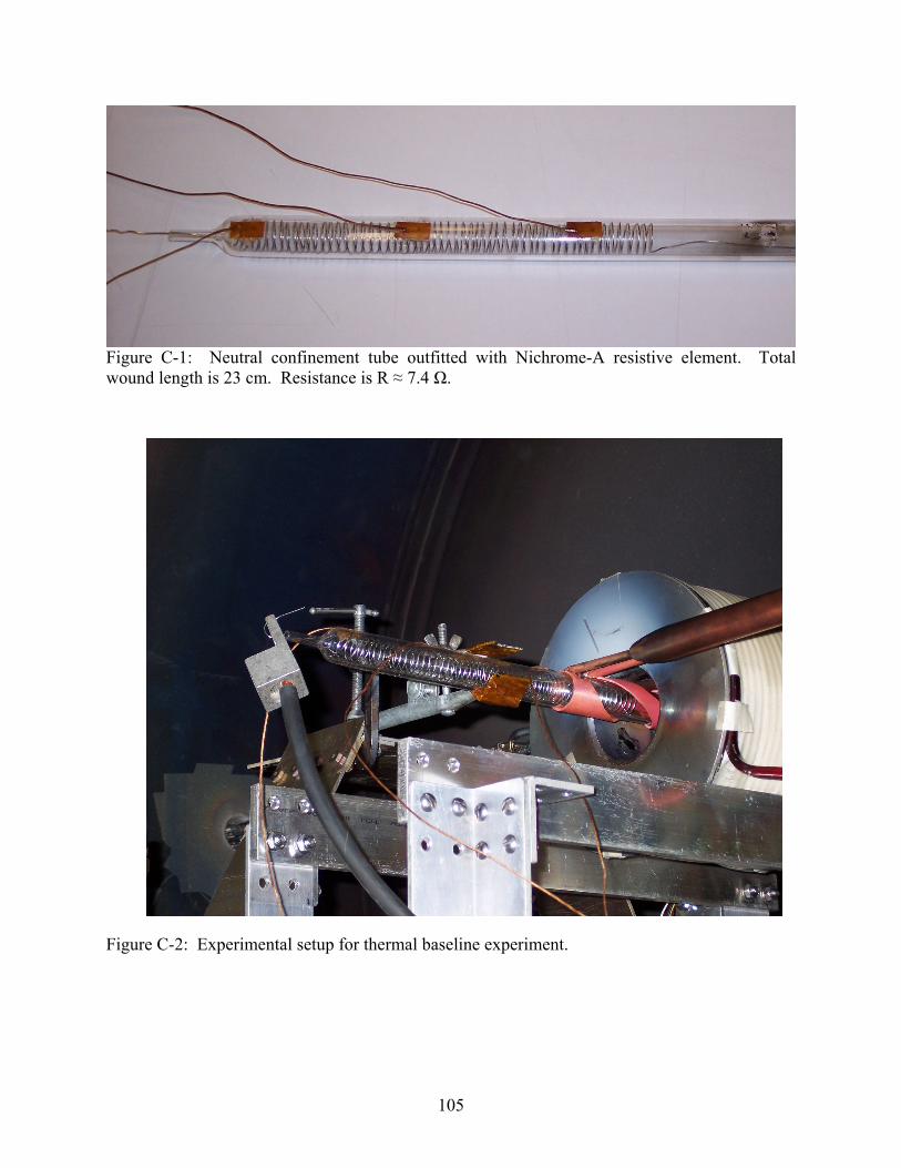
105
Figure C-1: Neutral confinement tube outfitted with Nichrome-A resistive element. Total
wound length is 23 cm. Resistance is R ≈ 7.4 Ω.
Figure C-2: Experimental setup for thermal baseline experiment.
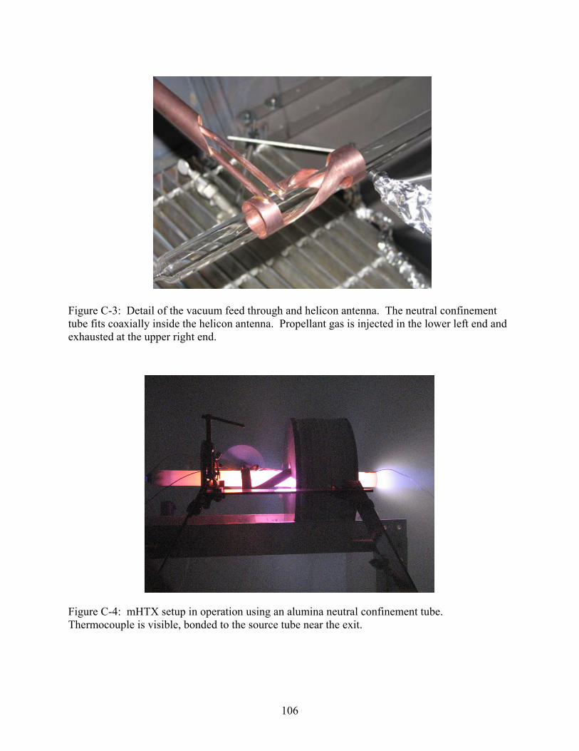
106
Figure C-3: Detail of the vacuum feed through and helicon antenna. The neutral confinement
tube fits coaxially inside the helicon antenna. Propellant gas is injected in the lower left end and
exhausted at the upper right end.
Figure C-4: mHTX setup in operation using an alumina neutral confinement tube.
Thermocouple is visible, bonded to the source tube near the exit.

107
References [1]Tikhonravov, M. K., (ed.), Works on Rocket Technology by E. K. Tsiolkovsky, Publishing House of the
Defense Ministry, Moscow, 1947; translated from the 1947 Russian text by NASA as NASA TT F-243,
1965.
[2] E. Stulinger, Ion Propulsion for Space Flight, Chapter 1, McGraw Hill Book Company, New York,
1964.
[3] H. Oberth, Wege zur Raumschiffahrt (Ways to Spaceflight), Harper & Row Publishers Inc., New York,
1957.
[4] L. R. Shepard, A. V. Cleaver, “The Atomic Rocket,” J. Brit. Interplanetary Society, Vol. 7, pp. 185,
1948, Vol. 8 pp. 23, 50, 1950.
[5] E. Stulinger, “Possibilities of Electrical Space Ship Propulsion,” Ber. 5th Intern. Astronaut. Congr.,
Innsbruck, pp. 100, August 1954.
[6] E. Stulinger, “Electrical Propulsion Systems for Space Ships with Nuclear Power Sources,” J.
Astronaut., Vol. 2 pp. 149, 1955, Vol. 3 pp.11, 33, 1956.
[7] E. Stulinger, “Flight Path of an Electrically Propelled Space Ship,” Jet Propulsion, Vol. 27, No. 4, pp.
410, April 1957.
[8] R. J. Cybulski, et al., “Results from SERT-I Ion Rocket Flight Test,” NASA Technical Note, D-2718,
1965.
[9] M.D. Rayman, P. Varghese, D.H. Lehman and L.L. Livesay, “Results from the Deep Space 1
Technology Validation Mission,” Acta Astronautica, Vol.47, p.475, 2000.
[10] H. Kuninaka, K. Nishiyama, I. Funaki, Y. Shimizu, T. Yamada and J. Kawaguchi, “Assessment of
Plasma Interactions and Flight Status of the HAYABUSA Asteroid Explorer Propelled by Microwave
Discharge Ion Engines,” IEEE Transactions on Plasma Science, Vol. 34 No. 5 Part 2, pp. 2125 – 2132,
October 2006.
[11] C.R. Koppel, F. Marchandise, M. Prioul, D. Estublier and F. Darnon, “The SMART-1 Electric
Propulsion Subsystem around the Moon: In Flight Experience”, AIAA 2005-3671, 42st Joint Propulsion
Conference, Tucson, July 2005.
108
[12] J. Brophy, C. Garner, B. Nakazono, M. Marcucci, M. Henry and D. Noon, “The Ion Propulsion
System For Dawn,”AIAA-2003-4542 39th AIAA/ASME/SAE/ASEE Joint Propulsion Conference and
Exhibit, Huntsville, Alabama, July 20-23, 2003
[13] R. G. Jahn, Physics of Electric Propulsion, Dover Publications Inc., New York, 1968
[14] P. W. Garrison, J. F. Stocky, “Future Spacecraft Propulsion,” AIAA Propulsion and Power Vol. 4, pp.
520 – 525, 1988
[15] D. K. Huzel, D. H. Huang, Modern Engineering for Liquid-Propellant Rocket Engines, Progress in
Astronautics and Aeronautics Vol. 147, American Institute of Aeronautics and Astronautics, Washington
D.C.,
[16] M. Martinez-Sanchez, J. E. Pollard “Spacecraft Electric Propulsion – An Overview,” AIAA Journal of
Propulsion and Power, Vol. 14 No. 5, 1998
[17] W. Finkelnburg, H. Maecker, “Electric Arcs and Thermal Plasmas,” Handbuch der Physik, Vol. 22,
1956.
[18] R. W. Boswell Plasma production using a standing helicon wave. Physics Letters A, Volume 33,
Issue 7, 14 December 1970, Pages 457-458
[19] C. Charles, R.W. Boswell, "A plasma beam generator". PCT (International) June 19, 2003 following
Provisional Patent Application No PS3033/02, June 19, 2002.
[20] R. W. Boswell. Very efficient plasma generation by whistler waves near the lower hybrid frequency.
Plasma Physics and Controlled Fusion, 26(10):1147–1162, February 1984.
[21] F. F. Chen, “Plasma Ionization by Helicon Waves,” Plasma Phys. Control. Fusion, Vol. 33, No. 4, pp.
339, 1991
[22] F. F. Chen and D. D. Blackwell. Upper limit to landau damping in helicon discharges. Phys. Rev.
Letters, 82(13):2677–2680, March 1999.
[23] D. Arnush. The role of trivelpiece-gould waves in antenna coupling to helicon waves. Physics of
Plasmas, 7(7):3042–3050, July 2000.
[24] K. P. Shamrai. Stable modes and abrupt density jumps in a helicon plasma source. Plasma Sources
Science and Technology, 7:499, 1998.
[25] B. N. Breizman and A. V. Arefiev. Radially localized helicon modes in nonuniform plasma. Physical
Review Letters, 84:3863, 2000.
[26] M. I. Panevsky. Characterization of the Resonant Electromagnetic Mode in Helicon Discharges. PhD
Dissertation, University of Texas, December 2003
[27] O.Batishchev, K.Molvig, Study of Operational Regimes of the VASIMR Helicon Plasma Source,
DPP/ICPP 2000 Meeting, Quebec City, Canada, Bull. APS 45 (7) 130, 2000.
109
[28] J. E. Palaia, “Empirical Aspects of a Mini-Helicon Plasma Thruster Experiment (mHTX@MIT),”
M.S. Thesis, MIT Aero/Astro, June 2006.
[29] M. Celik, “Experimental and Computational Studies of Electric Thruster Plasma Radiation Emission,”
Ph.D. Thesis, MIT Aero/Astro, May 2007
[30] J. M. Pucci, “An Analysis of Energy Balance in a Helicon Plasma Source for Space Propulsion,” M.S.
Thesis, MIT Aero/Astro, May 2007
[31] N. Sinenian, “Propulsion Mechanisms in a Helicon Plasma Thruster,” M.S. Thesis, MIT Aero/Astro,
February 2008
[32] A. R. Ellingboe, R. W. Boswell, “Capacitive, Inductive and Helicon-Wave Modes of Operation of a
Helicon Plasma Source,” Phys. Plasmas, Vol. 3, No. 7, 1996
[33] D. K. Cheng, Fundamentals of Engineering Electromagnetics, Addison-Wesley Publishing Company,
Inc., July 1993.
[34] G. G. Raju “Electron-Atom Collision Cross Sections in Argon: An Analysis and Comments,” IEEE
Transactions on Dielectrics and Electrical Insulation, Vol. 11 No. 4, Aug. 2004, pp. 649 - 673
[35] R. S. Brusa, G. P. Karwasz and A. Zecca, “Analytical Partitioning of Total Cross Sections for Electron
Scattering on Noble Gases,” Z. Phys. D, Vol. 38, pp. 279-287, 1996
[36] E. Krishnakumar and S. K. Srivastava, ‘‘Ionization Cross Sections of Rare Gas Atoms by Electron
Impact’’, J. Phys. B: At. Mol. Phys., Vol. 21, pp. 1055_1082, 1988.
[37] F. J. de Heer, R. H. J. Jansen and W. van der Kaay, “Total Cross Sections for Electron Scattering by
Ne, Ar, Kr and Xe,” J. Phys. B: At. Mol. Phys., Vol. 22, pp 979-1002, 1979.
[38] R. W. Boswell, “Very Efficient Plasma Generation by Whistler Waves Near the Lower Hybrid
Frequency,” Plasma Phys. Controlled Fusion 26, 1147 1984.
[39] L. Minnhagen, J. Opt. Soc. Am. 61, 1257 (1971)
[40] L. Minnhagen, J. Opt. Soc. Am. 63, 1185 (1973)
[41] I. Velchev, W. Hogervorst, and W. Ubachs, J. Phys. B 32, L511 (1999)
[42] Lawrence Berkley National Laboratory, Advanced Light Source Group DOE Contract DE-AC02-
05CH11231, July 2006