Embed Size (px)
Citation preview
11
Process dynamics
In a dynamic system, the values of the variables change with time, and in this chapter
we quantify the well-known fact that “things take time.” We also consider dynamic
modeling, dynamic responses (analysis), dynamic simulation (numerical calculation) and
process control.
11.1 Introduction
Some reasons for considering a system’s dynamics and obtaining dynamic models are:
1. To describe the time behavior of a batch process.2. To describe the transient response of a continuous process (e.g., dynamic change
from one steady state to another).3. To understand the dynamics of the process (analysis), for example, as expressed by
the time constant.4. To develop a “training simulator” for operator training.5. For “what occurs if” studies, for example, as a tool in a HAZOP analysis (“what
happens if this valve is closed?”).6. For optimization and control (control structure, tuning of controllers, model-based
control).
Note that when it comes to dynamics, there is no difference between a model for abatch process a continuous process.
The dynamic models we consider in this chapter are given in the form of differentialequations,
dy
dt= f(y, u) (11.1)
where u is the independent variable and y the dependent variable, as seen from acause-and-effect relationship. With a dynamic model, it is possible, given the system’sinitial state (y(t0) = y0) and given the value of all of the independent variables (u(t)for t > t0), to compute (“simulate”) the value of the dependent variables as a functionof time (y(t) for t > t0).
Up to now, we have studied steady-state behavior, where time t was not a variable.The steady-state model f(y, u) = 0 gives the relationship between the variables u andy for the special case when dy/dt = 0 (“the system is at rest”).
The basis for a dynamic model can be
274 CHEMICAL AND ENERGY PROCESS ENGINEERING
1. Fundamental: From balance equations + physics/chemistry; see the next section2. Empirical (regression-based): From experimental data (measurements)
Often we use a combination, where the parameters of a fundamental model areobtained from experimental measurement data.
Comment on notation. The dot notation (X) is used other places in this bookto indicate rate variables (e.g., m [kg/s] denotes the mass flow rate). However, inother fields and books, particularly in control engineering, the dot notation indicatestime derivative (that is m ≡ dm/dt). Since we work, in this chapter, with bothtime derivatives and rates, we here choose to avoid the dot notation altogether. Thefollowing special symbols are instead used for rates (amount of stream per unit oftime):
• Molar flow rate: F ≡ n [mol/s]• Mass flow rate: w ≡ m [kg/s]• Volumetric flow rate: q ≡ V [m3/s]
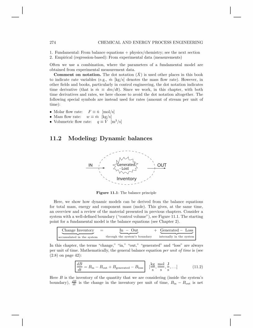
11.2 Modeling: Dynamic balances
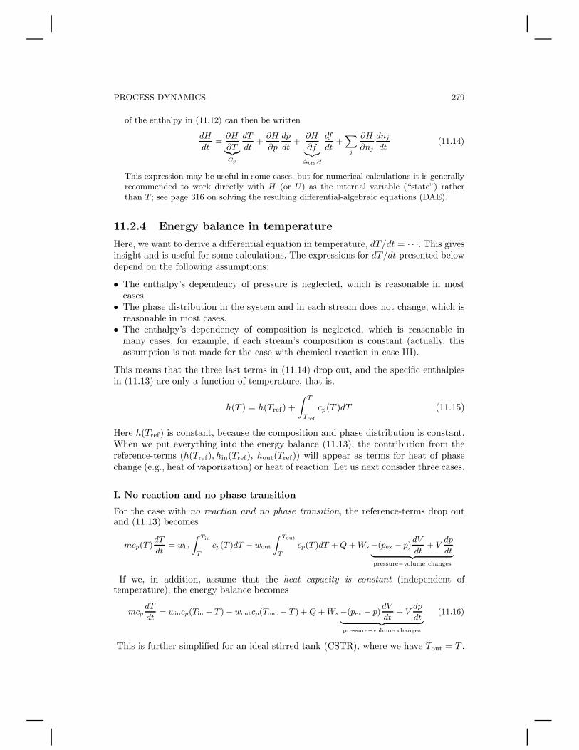
Inventory
Generated OUT- Lost
Figure 11.1: The balance principle
Here, we show how dynamic models can be derived from the balance equationsfor total mass, energy and component mass (mole). This gives, at the same time,an overview and a review of the material presented in previous chapters. Consider asystem with a well-defined boundary (“control volume”), see Figure 11.1. The startingpoint for a fundamental model is the balance equations (see Chapter 2).
Change Inventory︸ ︷︷ ︸
accumulated in the system
= In − Out︸ ︷︷ ︸
through the system′s boundary
+ Generated − Loss︸ ︷︷ ︸
internally in the system
In this chapter, the terms “change,” “in,” “out,” “generated” and “loss” are alwaysper unit of time. Mathematically, the general balance equation per unit of time is (see(2.8) on page 42):
dB
dt= Bin − Bout + Bgenerated − Bloss [
kg
s,mol
s,J
s, . . .] (11.2)
Here B is the inventory of the quantity that we are considering (inside the system’sboundary), dB
dt is the change in the inventory per unit of time, Bin − Bout is net

PROCESS DYNAMICS 275
supplied through the system’s boundary (with mass flows or through the wall) andBgenerated − Bloss is net supplied internally in the system. For conserved quantities(mass and energy), we have Bgenerated = 0 and Bloss = 0. Component mass (mol) isnot conserved, so we have to include a term for “net generated in chemical reactions,”which represents the sum of “generated” and “lost.” Similarly, momentum (mechanicalenergy) is not conserved and we have to include a friction term.
In principle, the balance equations are easy to formulate, but we need to decide:
1. Which control volume (where do we draw the boundary for the quantity we arebalancing)?
2. Which balance (which quantity are we considering, for example, mass or energy)?
The answer to the last question is typically:
• Interested in mass, volume or pressure: mass balance• Interested in concentration: component balance• Interested in temperature: energy balance• Interested in the interaction between flow and pressure: Mechanical energy balance
(= momentum balance = Bernoulli = Newton’s second law) (in some of the examplesbelow, we use the static momentum balance where the term for acceleration isneglected).
11.2.1 Dynamic total mass balance
The total mass balance per unit of time is
dm
dt= win − wout [kg/s] (11.3)
where m [kg] is the system’s mass (“inventory of mass inside the control volume”),dm/dt [kg/s] is the change in mass inventory per unit of time and win−wout [kg/s] arethe mass flow rates for for the entering and exiting streams (bulk flow). By introducingthe density, we get
d(ρV )
dt= ρinqin − ρoutqout [kg/s]
where V [m3] is the system’s volume, qin [m3/s] and qout [m3/s] are the volumetricflow rates and ρ, ρin and ρout [kg/m3] are the (average) densities.
For liquid-phase systems, it can often be assumed that the density ρ is constant (thatis, ρ = ρin = ρout = constant), and the mass balance becomes a “volume balance”
Constant density :dV
dt= qin − qout [m3/s] (11.4)
Quotation marks are here used to show that volume is generally not a conservedquantity. In practice, it is often the liquid level (or height h [m]) that is of interest.The relationship between volume and level is V = Ah for a tank with constant crosssection area A [m2], and more generally V =
∫A(h)dh when A varies with height. We
then getdV
dt= A
dh
dt+ h
∂A
∂h
dh
dt
276 CHEMICAL AND ENERGY PROCESS ENGINEERING
where the last term is zero for a constant cross section area A (since ∂A/∂h = 0).Note that the total number of moles in the system is generally not a conserved
quantity, that is, the total mole balance is
dn
dt= Fin − Fout + G [mol/s] (11.5)
where G [mol/s] is the net generated number of moles in chemical reactions.
11.2.2 Dynamic component balance
The dynamic component balance can, for an arbitrary component A, be written
dnA
dt= FA,in − FA,out + GA [mol A/s] (11.6)
(we normally use mole basis, but the component balance can also be written on weightbasis [kg A/s]). Here, nA [mol A] is the inventory (amount) of component A insidethe system’s boundary, FA,in − FA,out [mol A/s] are the molar flow rates of A in thestreams (bulk flow) and GA [mol A/s] is net generated in the chemical reactions. Thiscan, from (3.7), be calculated from
GA =∑
j
νA,jξj [mol A/s]
where νA,j is the stoichiometric coefficient for component A in reaction j, and ξj
[mol/s] is the extent of reaction for reaction j. Instead of the extent of reaction, onecan alternatively use the reaction rate, and from (10.7), write
GA =
∫ V
0
∑
j
νA,jrj
︸ ︷︷ ︸
rA
dV [mol A/s] (11.7)
where rj [mol/ m3 s] is the reaction rate for reaction j. Note that we in the dynamiccase usually do not restrict ourselves to independent reactions because this makesit more difficult to introduce the reaction rate. The reaction rate is a function ofconcentration and composition, and generally varies with the position in the reactor(and therefore the integral in (11.7)).
For example, for a first-order reaction A → B, we can have that
r = k(T )cA [mol A/s m3]
Here, we have rA = −r, where the sign is negative because A is consumed in thereaction and the stoichiometric coefficient is νA = −1. We often assume that thetemperature dependency of the reaction rate constant k follows Arrhenius’ equation
k(T ) = Ae−E/RT
where A is a constant and E [J/mol] is the activation energy. We also introduce
cA = nA/V ; cA,in = FA,in/qin; cA,out = FA,out/qout

PROCESS DYNAMICS 277
where cA [mol/m3] is the average concentration of A in the reactor. Similarly, theaverage reaction rate is defined rA = (
∫rAdV )/V . Then GA = rAV and the
component balance can be written
d(cAV )
dt= cA,inqin − cA,outqout + rAV [mol A/s] (11.8)
Here we have used concentration c, but we may alternatively use mole fraction orweight fraction.
Example 11.1 Ideal continuous stirred tank reactor (CSTR). Here we have perfectmixing and we do not need to use average values, that is, cA = cA and rA = rA. Furthermore,we have that cA,out = cA and the component balance (11.8) is
d(cAV )
dt= cA,inqin − cAqout + rAV (11.9)
If we, in addition, assume constant density ρ, we can introduce the “volume balance”(11.4) such that the left side of (11.9) is
d(cAV )
dt= cA
dV
dt+ V
dcA
dt= cA(qin − qout) + V
dcA
dt
The “out term” in (11.9) then drops out and the component balance for a CSTR becomes
VdcA
dt= (cA,in − cA)qin + rAV [mol A/s] (11.10)
Note that, with the assumption of constant density, this equation applies even if the reactorvolume V varies.
With a little practice, the balance (11.10) may be set up directly: “The concentrationchange in a CSTR is driven by the inflow having a different composition plus thecontribution for chemical reaction.” However, it is generally recommended to startfrom equation (11.6).
11.2.3 Dynamic energy balance
The general energy balance (4.10) over a time period ∆t with ∆U = Uf − U0 gives,as ∆t → 0, the dynamic energy balance:
dU
dt= Hin − Hout + Q + Ws − pex
dV
dt[J/s] (11.11)
Here, U [J] is the internal energy for the system (inside the control volume), whileHin − Hout is the sum of internal energy in the streams plus the flow work that thestreams perform on the system as they are “pushed” in or out of the system. The term−pex
dVdt is the work supplied to the system when its volume changes; it is negligible for
most systems. Q [J/s] is supplied heat (through the system’s wall), while Ws [J/s] issupplied useful mechanical work (usually shaft work, for example, from a compressor,pump or turbine). Note that there is no term of the kind “heat generated in chemical

278 CHEMICAL AND ENERGY PROCESS ENGINEERING
reaction” because the heat of reaction is indirectly included in the internal energy,and thus in the terms dU/dt, Hin, and Hout.
“Complete” general energy balance. Note that I, as before, have been a bit lazywhen writing the energy balance in the “general” form in (11.11). When necessary,terms for kinetic and potential energy must be added to U and H , and other workterms such as electrochemical work Wel must be included. Thus, as stated in the“energy balance reading rule” on page 4.4:
• Shaft work Ws [J/s] really means Ws + Wel+ other work forms.• Internal energy U of the system [J] really means E = U + EK + EP + other energy
forms. Here EK is kinetic energy and EP is potential energy of the system.• Enthalpy H of the in- and outstreams [J/s] really means H + EK + EP + other
energy forms. For a stream, EK = wαv2/2 and EP = wgz, see page 125, where w[kg/s] is the flow rate.
Energy balance in enthalpy
We usually prefer to work with enthalpy, and introducing U = H − pV in (11.11),gives
dH
dt= Hin − Hout + Q + Ws −(pex − p)
dV
dt+ V
dp
dt︸ ︷︷ ︸
pressure−volume changes
[J/s] (11.12)
Here, H = mh [J] is the enthalpy of the system (inside the control volume), where m[kg] is system mass and h [J/kg] is its specific enthalpy.
Comments:
1. The term “pressure-volume changes” in (11.12) and (11.13) is often negligible.
• The term is exactly zero (also for gases) for cases with constant pressure and volume.• The term is exactly zero (also for gases) for cases where the pressure is constant and
equal to the surrounding’s pressure (p = pex=constant).• Even with varying pressure, the term is approximately zero for liquids and solids,
because the volume V is relatively small for such systems.
However, the term “pressure-volume changes” can be considerable for gases with varyingpressure, for example, for a gas pipeline.
2. We have dHdt
= m dhdt
+h dmdt
and by introducing the mass balance (11.3), the energy balanceon “mass flow basis” becomes
mdh
dt= win(hin − h) − wout(hout − h) + Q + Ws −(pex − p)
dV
dt+ V
dp
dt| {z }
pressure−volume changes
[J/s] (11.13)
3. All enthalpies must refer to a common reference state. If we use, for example, the elementsat 298 K and 1 bar as the reference, the enthalpy H (or h) is the sum of (1) chemicalformation energy, (2) “latent” phase transition energy (if the phase differs from thestandard state), (3) thermal energy (“sensitive heat cp”), (4) mixing energy and (5)pressure-correction energy; see page 364.
4. Enthalpy H(T, p, f, nj) [J/kg] is generally a function of temperature T , pressure p, phasedistribution f (where f is fraction of light phase) and composition (nj). The time derivative
PROCESS DYNAMICS 279
of the enthalpy in (11.12) can then be written
dH
dt=
∂H
∂T|{z}
Cp
dT
dt+
∂H
∂p
dp
dt+
∂H
∂f|{z}
∆trsH
df
dt+X
j
∂H
∂nj
dnj
dt(11.14)
This expression may be useful in some cases, but for numerical calculations it is generallyrecommended to work directly with H (or U) as the internal variable (“state”) ratherthan T ; see page 316 on solving the resulting differential-algebraic equations (DAE).
11.2.4 Energy balance in temperature
Here, we want to derive a differential equation in temperature, dT/dt = · · ·. This givesinsight and is useful for some calculations. The expressions for dT/dt presented belowdepend on the following assumptions:
• The enthalpy’s dependency of pressure is neglected, which is reasonable in mostcases.
• The phase distribution in the system and in each stream does not change, which isreasonable in most cases.
• The enthalpy’s dependency of composition is neglected, which is reasonable inmany cases, for example, if each stream’s composition is constant (actually, thisassumption is not made for the case with chemical reaction in case III).
This means that the three last terms in (11.14) drop out, and the specific enthalpiesin (11.13) are only a function of temperature, that is,
h(T ) = h(Tref) +
∫ T
Tref
cp(T )dT (11.15)
Here h(Tref) is constant, because the composition and phase distribution is constant.When we put everything into the energy balance (11.13), the contribution from thereference-terms (h(Tref), hin(Tref), hout(Tref)) will appear as terms for heat of phasechange (e.g., heat of vaporization) or heat of reaction. Let us next consider three cases.
I. No reaction and no phase transition
For the case with no reaction and no phase transition, the reference-terms drop outand (11.13) becomes
mcp(T )dT
dt= win
Z Tin
T
cp(T )dT − wout
Z Tout
T
cp(T )dT + Q + Ws −(pex − p)dV
dt+ V
dp
dt| {z }
pressure−volume changes
If we, in addition, assume that the heat capacity is constant (independent oftemperature), the energy balance becomes
mcpdT
dt= wincp(Tin − T ) − woutcp(Tout − T ) + Q + Ws −(pex − p)
dV
dt+ V
dp
dt| {z }
pressure−volume changes
(11.16)
This is further simplified for an ideal stirred tank (CSTR), where we have Tout = T .
280 CHEMICAL AND ENERGY PROCESS ENGINEERING
II. With phase transition
Let us consider a somewhat more complex case with phase transition, where we cannotuse (11.16), because the reference terms h(Tref) do not drop out of the energy balance.
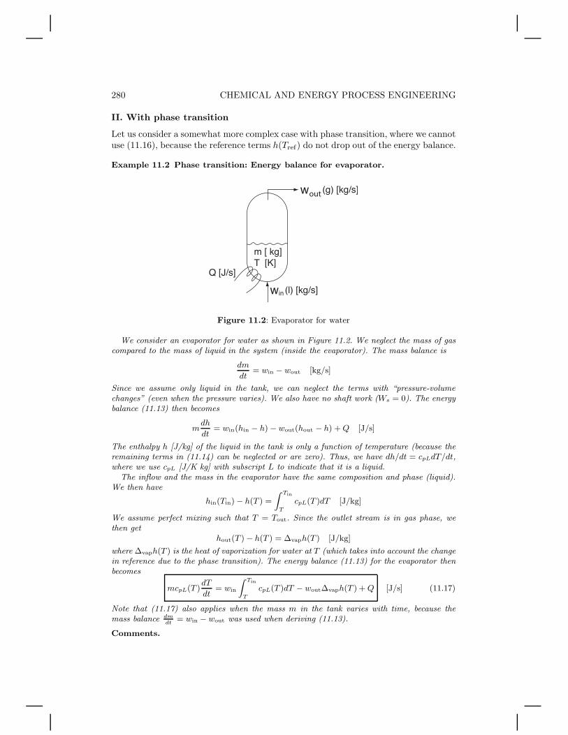
Example 11.2 Phase transition: Energy balance for evaporator.
w
w
out
Figure 11.2: Evaporator for water
We consider an evaporator for water as shown in Figure 11.2. We neglect the mass of gascompared to the mass of liquid in the system (inside the evaporator). The mass balance is
dm
dt= win − wout [kg/s]
Since we assume only liquid in the tank, we can neglect the terms with “pressure-volumechanges” (even when the pressure varies). We also have no shaft work (Ws = 0). The energybalance (11.13) then becomes
mdh
dt= win(hin − h) − wout(hout − h) + Q [J/s]
The enthalpy h [J/kg] of the liquid in the tank is only a function of temperature (because theremaining terms in (11.14) can be neglected or are zero). Thus, we have dh/dt = cpLdT/dt,where we use cpL [J/K kg] with subscript L to indicate that it is a liquid.
The inflow and the mass in the evaporator have the same composition and phase (liquid).We then have
hin(Tin) − h(T ) =
Z Tin
T
cpL(T )dT [J/kg]
We assume perfect mixing such that T = Tout. Since the outlet stream is in gas phase, wethen get
hout(T ) − h(T ) = ∆vaph(T ) [J/kg]
where ∆vaph(T ) is the heat of vaporization for water at T (which takes into account the changein reference due to the phase transition). The energy balance (11.13) for the evaporator thenbecomes
mcpL(T )dT
dt= win
Z Tin
T
cpL(T )dT − wout∆vaph(T ) + Q [J/s] (11.17)
Note that (11.17) also applies when the mass m in the tank varies with time, because themass balance dm
dt= win − wout was used when deriving (11.13).
Comments.

PROCESS DYNAMICS 281
1. The heat of vaporization is often given at a temperature Tref (for example, at the normalboiling point at 1 atm). The heat of vaporization at T can then be found by adding thefollowing subprocesses: (1) Cooling the liquid from T to Tref , (2) evaporation at Tref , and(3) heating the gas from Tref to T . We then get
∆vaph(T ) = ∆vaph(Tref) +
Z T
Tref
(cpV − cpL)dT
where ∆vaph(Tref) is the heat of vaporization at temperature Tref , and cpV is the heatcapacity of the steam.
2. Temperature and pressure are related by the equilibrium vapor pressure: p = psat(T ) (seepage 180).
With a little practice, it is possible to formulate energy balances of this kind directly:We imagine “standing in the tank” (the system) and use the temperature and phasehere as the reference. Then we consider what can be the source of changes in thesystem’s temperature. In the example with the evaporator, (11.17) can be derived asfollows:
“The temperature change in the tank (left side) is driven by the inflowhaving a different temperature than the tank (first term right side), andby enthalpy being removed by evaporation (second term) and by heat beingsupplied (third term).”
The term for the outlet stream drops out since it has the same temperature as thetank. More generally, it is recommended to start from the basic equations.
Exercise 11.1 Derive the energy balance for a flash tank with inventory n [mol], feed F[mol/s], vapor product D [mol/s] and liquid product B [mol/s] (make a flow sheet). Showthat it becomes
nCpLdT
dt= FCpL(TF − T ) + D · ∆vapH(T )
What are the units for the quantities in the equation? Which assumptions have been madewhen deriving this?
III. With chemical reaction
For cases with chemical reaction, it is usually most convenient to use a molar basis. Wereturn to (11.12) and introduce H(T, p, nj) =
∑
j njHm,j(T, p). Here, Hm,j [J/mol] isthe “partial molar enthalpy” for component j in the mixture. For cases with negligibleheat (enthalpy) of mixing, we have that Hm,j = Hm,j, where Hm,j is the molarenthalpy of pure component j in its actual phase. With this as a starting point, let usderive the general energy balance in terms of temperature (dT/dt) for a continuousstirred tank reactor (CSTR).
Example 11.3 Energy balance with temperature for CSTR. We consider an idealcontinuous stirred tank reactor (CSTR) where a chemical reaction takes place (Figure 11.3).Let us, as an example, consider the reaction 2A → B, but the derivation below is generaland applies to any reaction. The reaction rate is r(T, cA) [mol/s m3], and if we take intoconsideration the stoichiometry, the component balances are:
dnA
dt= FA,in − FA,out + νArV
| {z }
GA
[mol A/s]
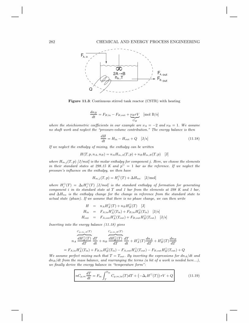
282 CHEMICAL AND ENERGY PROCESS ENGINEERING
out
outF
Figure 11.3: Continuous stirred tank reactor (CSTR) with heating
dnB
dt= FB,in − FB,out + νBrV
| {z }
GB
[mol B/s]
where the stoichiometric coefficients in our example are νA = −2 and νB = 1. We assumeno shaft work and neglect the “pressure-volume contribution.” The energy balance is then
dH
dt= Hin − Hout + Q [J/s] (11.18)
If we neglect the enthalpy of mixing, the enthalpy can be written
H(T, p, nA, nB) = nAHm,A(T, p) + nBHm,B(T, p) [J]
where Hm,j(T, p) [J/mol] is the molar enthalpy for component j. Here, we choose the elementsin their standard states at 298.15 K and p⊖ = 1 bar as the reference. If we neglect thepressure’s influence on the enthalpy, we then have
Hm,j(T, p) = H⊖j (T ) + ∆Htrs [J/mol]
where H⊖j (T ) = ∆fH
⊖j (T ) [J/mol] is the standard enthalpy of formation for generating
component i in its standard state at T and 1 bar from the elements at 298 K and 1 bar,and ∆Htrs is the enthalpy change for the change in reference from the standard state toactual state (phase). If we assume that there is no phase change, we can then write
H = nAH⊖A (T ) + nBH⊖
B (T ) [J]
Hin = FA,inH⊖A (Tin) + FB,inH⊖
B (Tin) [J/s]
Hout = FA,outH⊖A (Tout) + FB,outH
⊖B (Tout) [J/s]
Inserting into the energy balance (11.18) gives
nA
Cp,m,A(T )z }| {
dH⊖A (T )
dT
dT
dt+ nB
Cp,m,B(T )z }| {
dH⊖B (T )
dT
dT
dt+ H⊖
A (T )dnA
dT+ H⊖
B (T )dnB
dT
= FA,inH⊖A (Tin) + FB,inH⊖
B (Tin) − FA,outH⊖A (Tout) − FB,outH
⊖B (Tout) + Q
We assume perfect mixing such that T = Tout. By inserting the expressions for dnA/dt anddnB/dt from the mass balance, and rearranging the terms (a bit of a work is needed here...),we finally derive the energy balance in “temperature form”:
nCp,mdT
dt= Fin
Z Tin
T
Cp,m,in(T )dT +`−∆rH
⊖(T )´rV + Q (11.19)

PROCESS DYNAMICS 283
(For cases with many reactions, the term`−∆rH
⊖(T )´rV is replaced by
P
j
`−∆rH
⊖j (T )
´rjV ).
For our reaction 2A → B, we have
∆rH⊖(T ) =
X
j
νjH⊖j = H⊖
B − 2H⊖A [J/K mol] (11.20)
Furthermore,
n = nA + nB [mol]
Fin = FA,in + FB,in [mol/s]
and the molar heat capacities for the reactor (system) and feed are
Cp,m =nA
nCp,m,A(T ) +
nB
nCp,m,B(T ) [J/K mol]
Cp,m,in(T ) =FA,in
FinCp,m,A(T ) +
FB,in
FinCp,m,B(T ) [J/K mol]
Let us summarize the assumptions that have been made when deriving (11.19):
1. All streams have the same phase.2. Perfect mixing such that T = Tout.3. Heat of mixing is neglected.4. The pressure’s influence on the enthalpy is neglected.
Note that (11.19) applies to the case with varying composition in the reactor and a varyingamount of n (“holdup”) in the reactor. For a more detailed example with dynamic simulation,see page 311.
With a little experience, it is again possible to directly formulate the energy balance(11.19) in temperature form for a continuous stirred tank reactor:
“The temperature change in the reactor (left side) is driven by thedifference between the feed and reactor temperatures (first term left side),by the heat of reaction (second term) and by the supplied heat (thirdterm).”
Comments.
1. We note that the “heat of reaction” appears as a separate term when we choose towrite the energy balance in the “temperature form” in (11.19).
2. The energy balance in temperature form (11.19) gives interesting insights and isuseful in many situations. However, it is usually simpler for numerical calculations(dynamic simulation) to stay with the original form (11.11) or (11.12) with U orH as the state (differential) variables. See page 316 for solving the resulting DAEequations.
11.2.5 Steady-state balances
The dynamic balances derived above are all in the form dy/dt = f(y, u). We usuallyassume that the system is initially “at rest” (steady-state) with dy/dt = 0. The steady-state (nominal) values for u and y are here indicated by using superscript ∗, and wehave that f(y∗, u∗) = 0.
284 CHEMICAL AND ENERGY PROCESS ENGINEERING
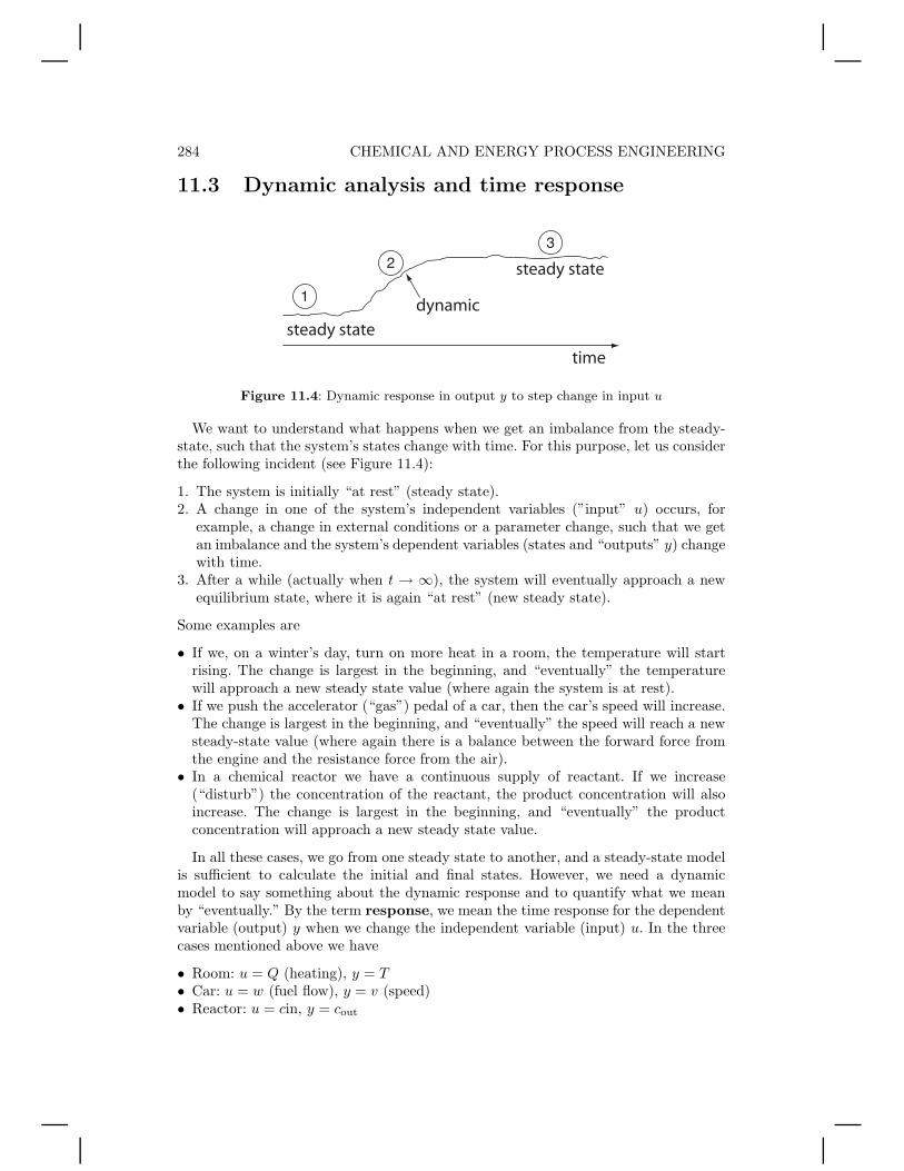
11.3 Dynamic analysis and time response
steady state
dynamic
steady state
time
Figure 11.4: Dynamic response in output y to step change in input u
We want to understand what happens when we get an imbalance from the steady-state, such that the system’s states change with time. For this purpose, let us considerthe following incident (see Figure 11.4):
1. The system is initially “at rest” (steady state).2. A change in one of the system’s independent variables (”input” u) occurs, for
example, a change in external conditions or a parameter change, such that we getan imbalance and the system’s dependent variables (states and “outputs” y) changewith time.
3. After a while (actually when t → ∞), the system will eventually approach a newequilibrium state, where it is again “at rest” (new steady state).
Some examples are
• If we, on a winter’s day, turn on more heat in a room, the temperature will startrising. The change is largest in the beginning, and “eventually” the temperaturewill approach a new steady state value (where again the system is at rest).
• If we push the accelerator (“gas”) pedal of a car, then the car’s speed will increase.The change is largest in the beginning, and “eventually” the speed will reach a newsteady-state value (where again there is a balance between the forward force fromthe engine and the resistance force from the air).
• In a chemical reactor we have a continuous supply of reactant. If we increase(“disturb”) the concentration of the reactant, the product concentration will alsoincrease. The change is largest in the beginning, and “eventually” the productconcentration will approach a new steady state value.
In all these cases, we go from one steady state to another, and a steady-state modelis sufficient to calculate the initial and final states. However, we need a dynamicmodel to say something about the dynamic response and to quantify what we meanby “eventually.” By the term response, we mean the time response for the dependentvariable (output) y when we change the independent variable (input) u. In the threecases mentioned above we have
• Room: u = Q (heating), y = T• Car: u = w (fuel flow), y = v (speed)• Reactor: u = cin, y = cout
PROCESS DYNAMICS 285
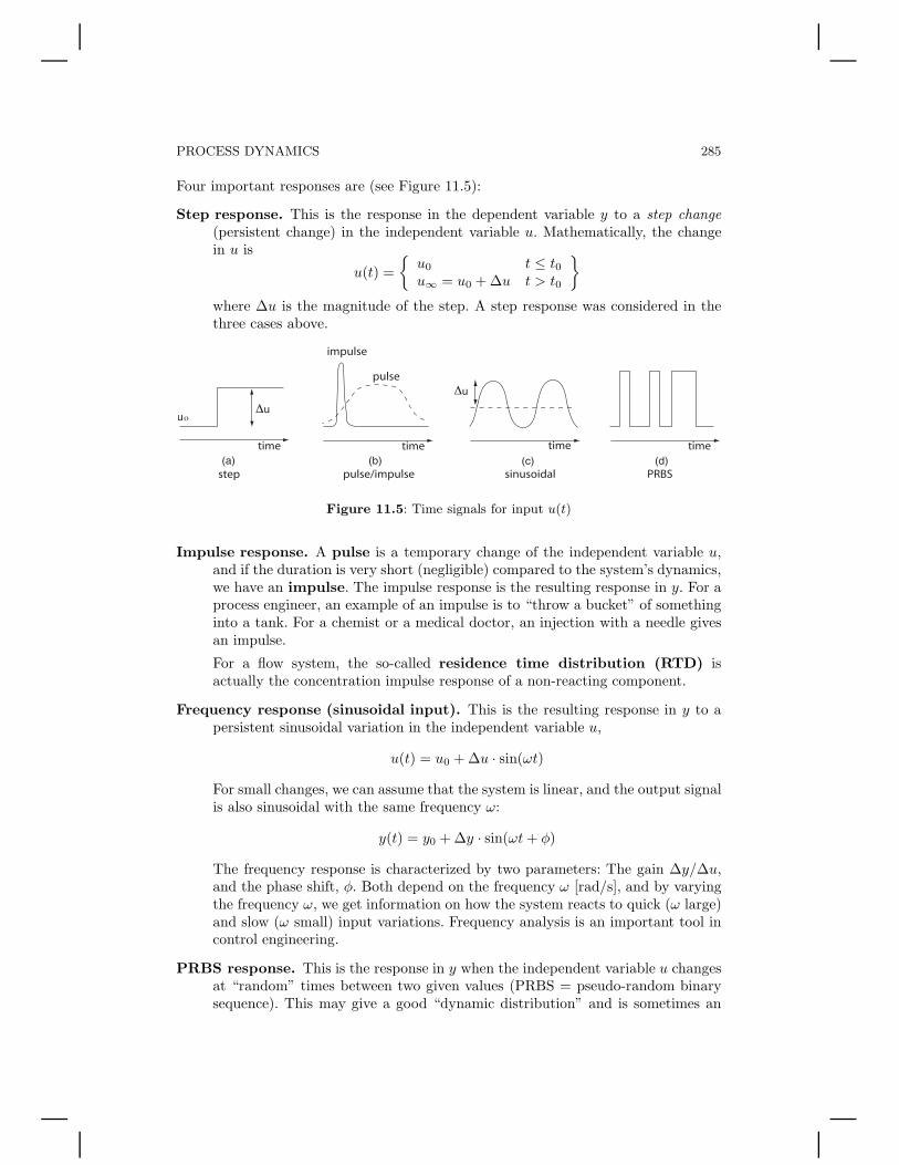
Four important responses are (see Figure 11.5):
Step response. This is the response in the dependent variable y to a step change(persistent change) in the independent variable u. Mathematically, the changein u is
u(t) =
{u0 t ≤ t0u∞ = u0 + ∆u t > t0
}
where ∆u is the magnitude of the step. A step response was considered in thethree cases above.
pulse/impulsestep
impulse
pulse
sinusoidal
time time time time
PRBS
Figure 11.5: Time signals for input u(t)
Impulse response. A pulse is a temporary change of the independent variable u,and if the duration is very short (negligible) compared to the system’s dynamics,we have an impulse. The impulse response is the resulting response in y. For aprocess engineer, an example of an impulse is to “throw a bucket” of somethinginto a tank. For a chemist or a medical doctor, an injection with a needle givesan impulse.
For a flow system, the so-called residence time distribution (RTD) isactually the concentration impulse response of a non-reacting component.
Frequency response (sinusoidal input). This is the resulting response in y to apersistent sinusoidal variation in the independent variable u,
u(t) = u0 + ∆u · sin(ωt)
For small changes, we can assume that the system is linear, and the output signalis also sinusoidal with the same frequency ω:
y(t) = y0 + ∆y · sin(ωt + φ)
The frequency response is characterized by two parameters: The gain ∆y/∆u,and the phase shift, φ. Both depend on the frequency ω [rad/s], and by varyingthe frequency ω, we get information on how the system reacts to quick (ω large)and slow (ω small) input variations. Frequency analysis is an important tool incontrol engineering.
PRBS response. This is the response in y when the independent variable u changesat “random” times between two given values (PRBS = pseudo-random binarysequence). This may give a good “dynamic distribution” and is sometimes an
286 CHEMICAL AND ENERGY PROCESS ENGINEERING
effective method for obtaining experimental data that can be used for estimating(=“identify” in control engineering) parameters in an empirical dynamic modelfor the relationship between u and y.
The step response is very popular in process engineering because it is simple toperform, understand and analyze. In the following, we study the step response inmore detail.
11.3.1 Step response and time constant
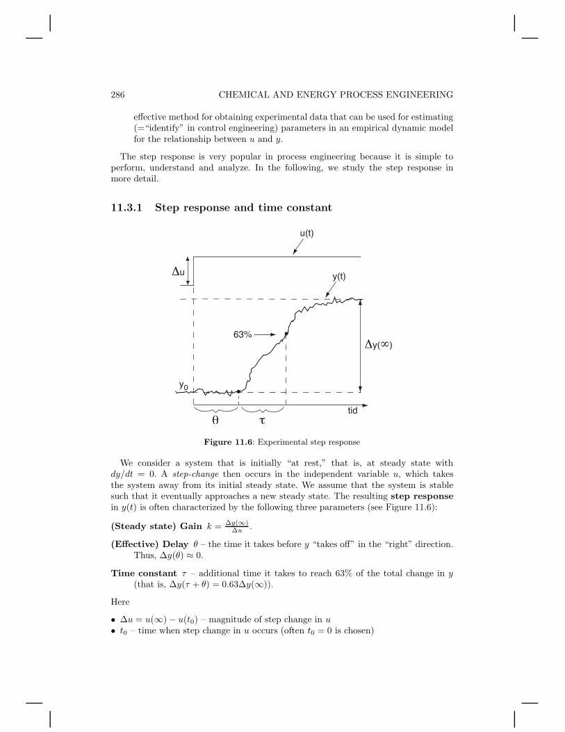
Figure 11.6: Experimental step response
We consider a system that is initially “at rest,” that is, at steady state withdy/dt = 0. A step-change then occurs in the independent variable u, which takesthe system away from its initial steady state. We assume that the system is stablesuch that it eventually approaches a new steady state. The resulting step responsein y(t) is often characterized by the following three parameters (see Figure 11.6):
(Steady state) Gain k = ∆y(∞)∆u .
(Effective) Delay θ – the time it takes before y “takes off” in the “right” direction.Thus, ∆y(θ) ≈ 0.
Time constant τ – additional time it takes to reach 63% of the total change in y(that is, ∆y(τ + θ) = 0.63∆y(∞)).
Here
• ∆u = u(∞) − u(t0) – magnitude of step change in u• t0 – time when step change in u occurs (often t0 = 0 is chosen)
PROCESS DYNAMICS 287
• ∆y(t) = y(t) − y(t0) – the resulting change in y• y(t0) = y0 – initial (given) steady state• y(∞) – final (new) steady state
The value of ∆y(∞) = y(∞)− y(t0), and thereby of the steady state gain k, can bedetermined from a steady state model, if one is available.
The cause of the delay (time delay) θ may be a transport delay (for example a pipe)or a delay in a measurement, but in most cases it represents the contribution frommany separate dynamic terms that, altogether, give a response that resembles a delay(hence the term “effective” delay).
The time constant τ characterizes the system’s dominant “inertia” against changes.It is defined as the additional time (after the time delay) it takes the variable to reach63% (more precisely, a fraction 1 − e−1 = 1 − 0.3679 ≈ 0.63, see below) of its totalchange. Why do we not let the time constant be the time it takes to reach all (100%)of its change? Because it generally take an infinitely long time for the system to reachexactly its final state, so this would not give a meaningful value.
The values of the parameters k, τ and θ are independent of the size of the step(independent of the value of ∆u), provided the step ∆u is sufficiently small such thatwe remain in the “linear region.” On page 301, we show how we can derive a linearmodel.
11.3.2 Step response for first-order system
The basis for the definition of τ given above is the simplest case with one lineardifferential equation (first-order system). Here, we study this system in more detail.A first-order system can be written in the following standard form
τdy
dt= −y + ku , y(t0) = y0 (11.21)
where
• u is the independent variable (input)• y is the dependent variable (output)• τ is the time constant• k is the gain
We now assume that
1. The system is “at rest” at time t0 with dy/dt = 0, that is, for t ≤ t0 we have u = u0
and y0 = ku0.2. The independent variable u changes from u0 to a constant value u = u0 + ∆u at
time t0.
As proven below, the solution (“step response”) can then be written as
y(t) = y0 +(
1 − e−t/τ)
k∆u (11.22)
or∆y(t)︸ ︷︷ ︸
y(t)−y0)
= ∆y(∞)︸ ︷︷ ︸
y(∞)−y0
(
1 − e−t/τ)
(11.23)

288 CHEMICAL AND ENERGY PROCESS ENGINEERING
Initial slope crosses final value at (time constant)
of change
time
Figure 11.7: Step response for first-order system
(you should try to remember this one). k is the steady state gain, and when t → ∞ wehave e−t/τ → 0 and the system approaches a new steady state where ∆y(∞) = k∆u.Notet that the exponential term 1 − e−t/τ describes how fast the system approachesits new steady state, and as a function of the non-dimensional time t/τ we have:
t/τ 1 − e−t/τ Value Comment
0 1 − e0 = 00.1 1 − e−0.1 = 0.0950.5 1 − e−0.5 = 0.3931 1 − e−1 = 0.632 63% of change is reached after time t = τ2 1 − e−2 = 0.8653 1 − e−3 = 0.9504 1 − e−4 = 0.982 98% of change is reached after time t = 4τ5 1 − e−5 = 0.993∞ 1 − e−∞ = 1
The time response is plotted in Figure 11.7. We note that at time t = τ (the timeconstant), we have reached 63% of the total change, and after four time constants, wehave reached 98% of the change (and we have for all practical purposes arrived at thenew steady state). Note also from Figure 11.7 that the initial slope of the response (attime t = 0) goes through to the point (τ, y(∞)). This can be shown mathematicallyfrom (11.23):
dy
dt= (y(∞) − y0)
1
τe−t/τ ⇒
(dy
dt
)
t=0
=y(∞) − y0
τ(11.24)
This means that the response y(t) would reach the final value y(∞) at time τ if itcontinued unaltered (in a straight line) with its initial slope.
Comments.1. As seen from the proof below, (11.23) applies also to cases where the system is not
initially at rest. This is not the case for (11.22).

PROCESS DYNAMICS 289
2. For cases where τ is negative, the system is unstable, and we get that y(t) goes to infinitywhen t goes to infinity.
3. From (11.24) and ∆y(∞) = k∆u, we derive that
1
∆u
„dy
dt
«
t=0
=k
τ(11.25)
This means that the initial slope k′ of the “normalized” response ∆y(t)/∆u is equal to the
ratio k/τ , i.e., k′ , k/τ .
Proof: Step response for a first-order system
Consider a first-order system in standard form, (11.21),
τdy
dt= −y + ku; y(0) = y0 (11.26)
where both τ and ku are constant. There are many ways of solving the linear differential equation(11.26). We can for example use separation of variables and derive
dy
y − ku= −dt
τ
Integration givesZ y
y0
dy
y − ku=
Z t
0−dt
τ⇒ ln
y − ku
y0 − ku= − t
τ
and we get the general solution
y(t) = ku + e−t/τ (y0 − ku)
We subtract y0 from both sides and get
y(t) − y0 =“
1 − e−t/τ”
(ku − y0) (11.27)
Since e−t/τ → 0 as t → ∞, we have that y(∞) = ku, and by introducing deviation variables
∆y(t) , y(t) − y(0) (11.28)
we find that (11.27) can be written in the following general form
∆y(t) = ∆y(∞)“
1 − e−t/τ”
(11.29)
We have so far not assumed that the system is “at rest” at t = t0, but let us do this now. We thenhave at t = t0 that dy/dt = 0, which gives
y0 = ku0
and (11.27) gives for a system that is initially at rest:
∆y(t)| {z }
y(t)−y0
=“
1 − e−t/τ”
k ∆u|{z}
u−u0
(11.30)
Example 11.4 Concentration response in continuous stirred tankWe consider the concentration response for component A in a continuous stirred tank
without chemical reaction (see Figure 11.8). We assume constant liquid density ρ and constantvolume V . The system is assumed to be at rest at t = 0. We want to find the step responsefor t > 0 given the following data
V = 5m3; q = 1m3/h
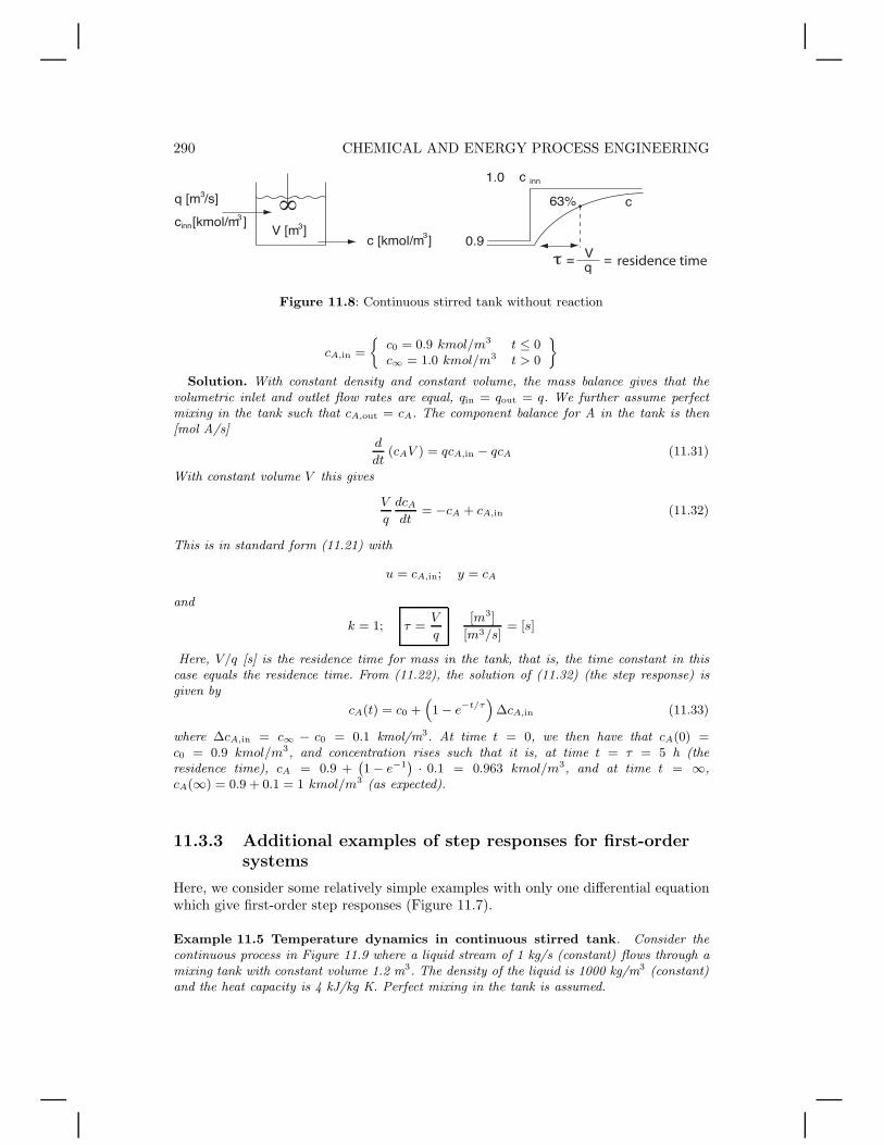
290 CHEMICAL AND ENERGY PROCESS ENGINEERING
residence time
Figure 11.8: Continuous stirred tank without reaction
cA,in =
c0 = 0.9 kmol/m3 t ≤ 0c∞ = 1.0 kmol/m3 t > 0
ff
Solution. With constant density and constant volume, the mass balance gives that thevolumetric inlet and outlet flow rates are equal, qin = qout = q. We further assume perfectmixing in the tank such that cA,out = cA. The component balance for A in the tank is then[mol A/s]
d
dt(cAV ) = qcA,in − qcA (11.31)
With constant volume V this gives
V
q
dcA
dt= −cA + cA,in (11.32)
This is in standard form (11.21) with
u = cA,in; y = cA
and
k = 1; τ =V
q
[m3]
[m3/s]= [s]
Here, V/q [s] is the residence time for mass in the tank, that is, the time constant in thiscase equals the residence time. From (11.22), the solution of (11.32) (the step response) isgiven by
cA(t) = c0 +“
1 − e−t/τ”
∆cA,in (11.33)
where ∆cA,in = c∞ − c0 = 0.1 kmol/m3. At time t = 0, we then have that cA(0) =c0 = 0.9 kmol/m3, and concentration rises such that it is, at time t = τ = 5 h (theresidence time), cA = 0.9 +
`1 − e−1
´· 0.1 = 0.963 kmol/m3, and at time t = ∞,
cA(∞) = 0.9 + 0.1 = 1 kmol/m3 (as expected).
11.3.3 Additional examples of step responses for first-ordersystems
Here, we consider some relatively simple examples with only one differential equationwhich give first-order step responses (Figure 11.7).
Example 11.5 Temperature dynamics in continuous stirred tank. Consider thecontinuous process in Figure 11.9 where a liquid stream of 1 kg/s (constant) flows through amixing tank with constant volume 1.2 m3. The density of the liquid is 1000 kg/m3 (constant)and the heat capacity is 4 kJ/kg K. Perfect mixing in the tank is assumed.

PROCESS DYNAMICS 291
residence time
Time
Figure 11.9: Temperature dynamics in continuous stirred tank without reaction
The process is initially operated at steady state such that the inlet temperature Tin is 50oCand the outlet temperature Tout = T is 50oC (so we assume no heat loss). Suddenly, thetemperature of the inflow is changed to 60 oC (step change). The outlet temperature will also“eventually” reach 60 oC. The question is: What is the time constant, that is, how long doesit take before the temperature in the tank (and outlet stream) has increased by 0.63·10 = 6.3oCto 56.3 oC?
Solution. Since the mass in the tank is constant, the mass balance gives wout = win =w = 1 kg/s. The energy balance (11.12) for the tank is (liquid)
dH
dt= Hin − Hout [J/s]
With the assumption of constant heat capacity cp, this gives
mcpdT
dt= wcp(Tin − T )
or equivalentlym
w
dT
dt= −T + 1 · Tin
With y = T and u = Tin we see that this is in standard form (11.21) with
τ =m
w=
ρV
w=
1000 · 1.2
1= 1200 s; k = 1
In other words, it will take τ = 1200 s = 20 min (the residence time m/w) before the outletstream’s temperature reaches 56.3 oC (and it will take an infinitely long time before it reaches60 oC).
Note that the time constant also for this example equals the residence time. This is true forchanges in both concentration and temperature for a continuous stirred tank without reactionor heating.
Example 11.6 Temperature dynamics in continuous stirred tank with heatexchange.
Consider the same example as above, where the inlet temperature is changed from 50oC (initial steady state) to 60 oC, but we have heating (see Figure 11.10) such that thetemperature in the tank is 70 oC (initial steady state). We consider the response and determinethe time constant for the following two cases:
1. An electric heater is used such that the supplied heat Q is independent of the temperatureT in the tank.
2. We have a heat exchanger with condensing stream on the hot side. The supplied heat isQ = UA(Th − T ) where Th (hot side temperature) is constant at 110 oC.

292 CHEMICAL AND ENERGY PROCESS ENGINEERING
changes from 50°C to 60°C
time
constant
Figure 11.10: Continuous stirred tank with heating
Solution. The energy balance (11.12) becomes [J/s]
mcpdT
dt= wcp(Tin − T ) + Q
At the initial steady state (dT/dt = 0), we have (before the change in Tin)
Q = −wcp(Tin − T ) = −1 kg/s · 4000 J/kg K · (50 − 70)K = 80000J/s = 80 kW
1. For the case when Q is independent of T , transformation to the standard form (11.21)gives that the time constant is τ = m/w = 1200 s (residence time), and that the gain fromTin to T is k = 1, that is, the steady-state temperature rise in the tank is 10 oC, that is,it will eventually rise to 80 oC.
2. For the case where Q depends on T , the energy balance becomes
mcpdT
dt= wcp(Tin − T ) + UA(Th − T ) (11.34)
and transformation to the standard form (11.21) gives
τ =mcp
wcp + UA; k =
wcp
wcp + UA
The time constant τ and the gain k are both smaller than in case 1. The reason is thatthe heat exchanger counteracts some of the temperature change (“negative feedback”).For numerical calculations, we need to know the value of UA. We have UA = Q/(Th−T ),and from the initial steady state data, we find UA = 80 ·103/(110−70) = 2000 W/K. Thetime constant and the gain are then
τ =mcp
wcp + UA=
1200 · 40001 · 4000 + 2000
= 800 s; k =4000
4000 + 2000= 0.67
that is, the temperature in the tank only increases by 6.7 oC to 76.7 oC – while in case 1with an electric heater it increased by 10 oC.
Although k and τ are different, we note that k′ = k/τ = 1/1200 is the same in both cases,and since from (11.25) limt→0∆T ′(t) = (k/τ ) ·∆Tin, this means that the initial responses arethe same (see also Figure 11.10). This is reasonable also from physical considerations, sincethe “counteracting” negative feedback effect from the heat exchanger only comes in after thetank temperature T starts increasing which leads to a reduction in Q = UA(Th − T ).

PROCESS DYNAMICS 293
Example 11.7 Dynamics of cooking plate. Let us consider a cooking plate with massm = 1 kg and specific heat capacity cp = 0.5 kJ/kg K. The cooking plate is heated byelectric power and the supplied heat is Q1 = 2000 W. The heat loss from the cooking plate isUA(T − To) where T is the cooking plate’s temperature, To = 290K is the temperature of thesurroundings, A = 0.04m2 and U is the overall heat transfer coefficient. If we leave the plateunattended, then we find that T → 1000K when t → ∞. What is the time constant for thecooking plate (defined as the time it takes to obtain 63% of the final temperature change)?
Solution. This is a closed system without mass flows and shaft work, and since the cookingplate is solid, we can neglect energy related to pressure-volume changes. The energy balance(11.12) around the cooking plate (the system) gives
dH
dt= Q
Here, there are two contributions to the supplied heat Q, from electric power and from heatloss, that is,
Q = Q1 − UA(T − To)
The enthalpy of the cooking plate is a function of temperature, that is, dH/dt = mcpdT/dt.The energy balance becomes
mcpdT
dt= Q1 − UA(T − To) (11.35)
In order to determine the overall heat transfer coefficient U , we use the steady statetemperature T ∗ = 1000K. At steady state, the energy balance is 0 = Q1 − UA(T ∗ − To)and we find
U =Q1
A(T ∗ − To)=
2000
0.04(1000 − 290)= 70.4 [W/m2 K]
We assume that the overall heat transfer coefficient U is constant during the heating. Thedynamic energy balance (11.35) is then a linear first-order differential equation which can bewritten in standard form
τdT
dt= −T + ku (11.36)
whereτ =
mcp
UA= 177.5 s
and
ku =1
UA|{z}
k1
Q1|{z}
u1
+ 1|{z}
k2
· T0|{z}
u2
In other words, we find that it takes time t = τ = 177.5 s (about 3 min) to obtain 63% of thefinal change of the cooking plate’s temperature.
Example 11.8 Response of thermocouple sensor in coffee cup. Temperature isoften measured with a thermocouple sensor based on the fact that electric properties areaffected by temperature. We have a thermocouple and a coffee cup and perform the followingexperiments:
1. Initially, we hold the thermocouple sensor in the air (such that it measures the airtemperature).
2. We put the thermocouple into the coffee (and keep it there for some time so that thethermocouple’s temperature is almost the same as the coffee’s temperature).
3. We remove it from the coffee (the temperature will decrease and eventually approach thetemperature of air – actually, it may temporarily be lower than the air temperature becauseof the heat required for evaporation of remaining coffee drops).
294 CHEMICAL AND ENERGY PROCESS ENGINEERING
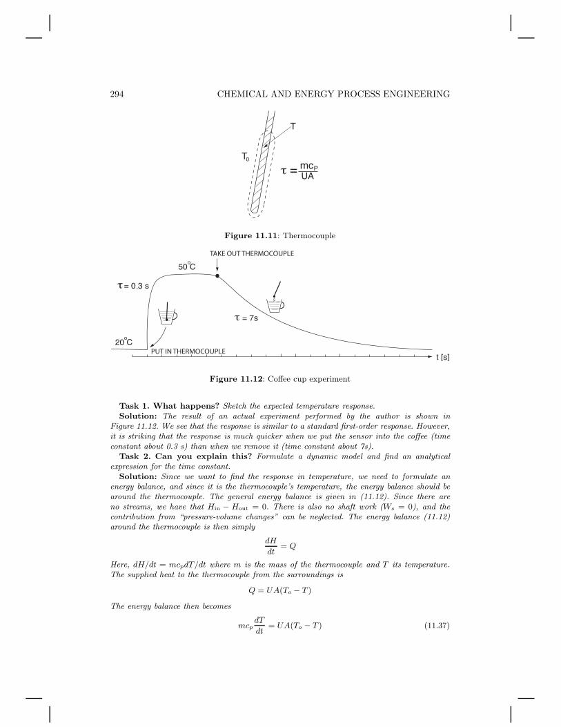
Figure 11.11: Thermocouple
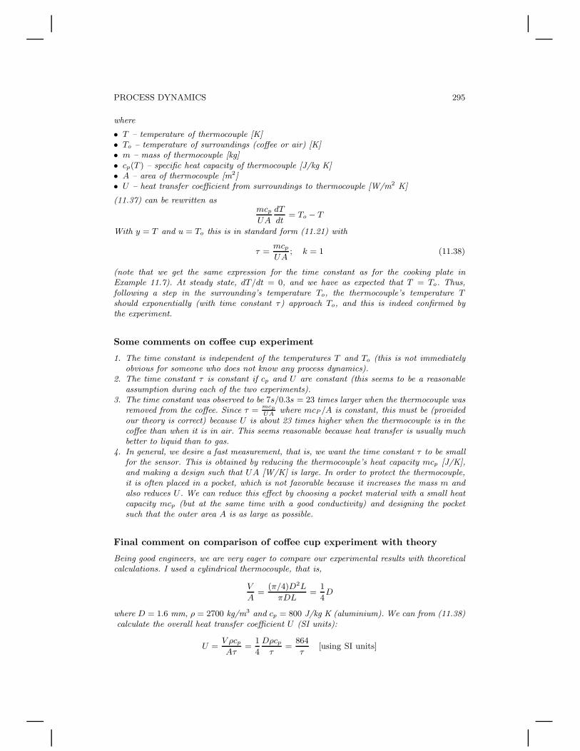
TAKE OUT THERMOCOUPLE
PUT IN THERMOCOUPLE
Figure 11.12: Coffee cup experiment
Task 1. What happens? Sketch the expected temperature response.Solution: The result of an actual experiment performed by the author is shown in
Figure 11.12. We see that the response is similar to a standard first-order response. However,it is striking that the response is much quicker when we put the sensor into the coffee (timeconstant about 0.3 s) than when we remove it (time constant about 7s).
Task 2. Can you explain this? Formulate a dynamic model and find an analyticalexpression for the time constant.
Solution: Since we want to find the response in temperature, we need to formulate anenergy balance, and since it is the thermocouple’s temperature, the energy balance should bearound the thermocouple. The general energy balance is given in (11.12). Since there areno streams, we have that Hin − Hout = 0. There is also no shaft work (Ws = 0), and thecontribution from “pressure-volume changes” can be neglected. The energy balance (11.12)around the thermocouple is then simply
dH
dt= Q
Here, dH/dt = mcpdT/dt where m is the mass of the thermocouple and T its temperature.The supplied heat to the thermocouple from the surroundings is
Q = UA(To − T )
The energy balance then becomes
mcpdT
dt= UA(To − T ) (11.37)
PROCESS DYNAMICS 295
where
• T – temperature of thermocouple [K]• To – temperature of surroundings (coffee or air) [K]• m – mass of thermocouple [kg]• cp(T ) – specific heat capacity of thermocouple [J/kg K]• A – area of thermocouple [m2]• U – heat transfer coefficient from surroundings to thermocouple [W/m2 K]
(11.37) can be rewritten asmcp
UA
dT
dt= To − T
With y = T and u = To this is in standard form (11.21) with
τ =mcp
UA; k = 1 (11.38)
(note that we get the same expression for the time constant as for the cooking plate inExample 11.7). At steady state, dT/dt = 0, and we have as expected that T = To. Thus,following a step in the surrounding’s temperature To, the thermocouple’s temperature Tshould exponentially (with time constant τ) approach To, and this is indeed confirmed bythe experiment.
Some comments on coffee cup experiment
1. The time constant is independent of the temperatures T and To (this is not immediatelyobvious for someone who does not know any process dynamics).
2. The time constant τ is constant if cp and U are constant (this seems to be a reasonableassumption during each of the two experiments).
3. The time constant was observed to be 7s/0.3s = 23 times larger when the thermocouple wasremoved from the coffee. Since τ =
mcp
UAwhere mcP /A is constant, this must be (provided
our theory is correct) because U is about 23 times higher when the thermocouple is in thecoffee than when it is in air. This seems reasonable because heat transfer is usually muchbetter to liquid than to gas.
4. In general, we desire a fast measurement, that is, we want the time constant τ to be smallfor the sensor. This is obtained by reducing the thermocouple’s heat capacity mcp [J/K],and making a design such that UA [W/K] is large. In order to protect the thermocouple,it is often placed in a pocket, which is not favorable because it increases the mass m andalso reduces U . We can reduce this effect by choosing a pocket material with a small heatcapacity mcp (but at the same time with a good conductivity) and designing the pocketsuch that the outer area A is as large as possible.
Final comment on comparison of coffee cup experiment with theory
Being good engineers, we are very eager to compare our experimental results with theoreticalcalculations. I used a cylindrical thermocouple, that is,
V
A=
(π/4)D2L
πDL=
1
4D
where D = 1.6 mm, ρ = 2700 kg/m3 and cp = 800 J/kg K (aluminium). We can from (11.38)calculate the overall heat transfer coefficient U (SI units):
U =V ρcp
Aτ=
1
4
Dρcp
τ=
864
τ[using SI units]
296 CHEMICAL AND ENERGY PROCESS ENGINEERING
Here, I found experimentally τ = 0.3s (coffee, that is, water) and τ = 7s (air), which givesU = 2880 W/m2 K (water) and U = 123 W/m2 K (air). Immediately, the value 2880 W/m2
K seems very high, because it is similar to values we find in heat exchangers with forcedconvection, and here we have natural convection. Let us compare with theoretical values fornatural convection to air and water. For natural convection,1 Nu = 0.5(Gr ·Pr)0.25, wherethe non-dimensional groups Nu, Gr and Pr are defined as
Nu =hD
k; Pr =
cpµ
k; Gr =
gβ∆TD3
(µ/ρ)2
Inserting and rearranging gives
h = 0.5
„k3cpρ2gβ
µ
«0.25
·„
∆T
D
«0.25
where k is the thermal conductivity, β the thermal expansion coefficient and µ theviscosity of the fluid. We use the following physical and transport data:
Air : k = 0.027W
K m; cp = 1000
J
kg K; µ = 1.8 · 10−5 kg
m s; ρ = 1.2
kg
m3;β =
1
T= 0.003
1
K
Water : k = 0.7W
K m; cp = 4200
J
kg K;µ = 10−3 kg
m s; ρ = 1000
kg
m3;β = 0.001
1
K
We then find for natural convection (SI units)
Air : h = 1.31 ·„
∆T
D
«0.25
Water : h = 173 ·„
∆T
D
«0.25
Note from this that with natural convection, the heat transfer coefficient h to water is morethan 100 times higher than to air. If we use D = 10−3 m and ∆T = 10 K (mean temperaturedifference between coffee and air; the exact value is not that important since it is raised tothe power 0.25) we get
`∆TD
´0.25= 10 (SI units) and if we assume U ≈ h (that is, we assume
that the heat conduction inside the thermocouple is very fast), we estimate theoretically thatU = 13.1 W/m2K (air) and U = 1730 W/m2K (water). We see that the theoretical U-value for water (1730 W/m2 K) is quite close to the experimental (2880 W/m2 K), while thetheoretical U-value for air (13.1 W/m2 K) is much lower than the experimental (123 W/m2
K) estimated from the experiment. The reason for this is probably remaining water dropletson the thermocouple which evaporate and improve the heat transfer for the case when weremove the thermocouple from the coffee.
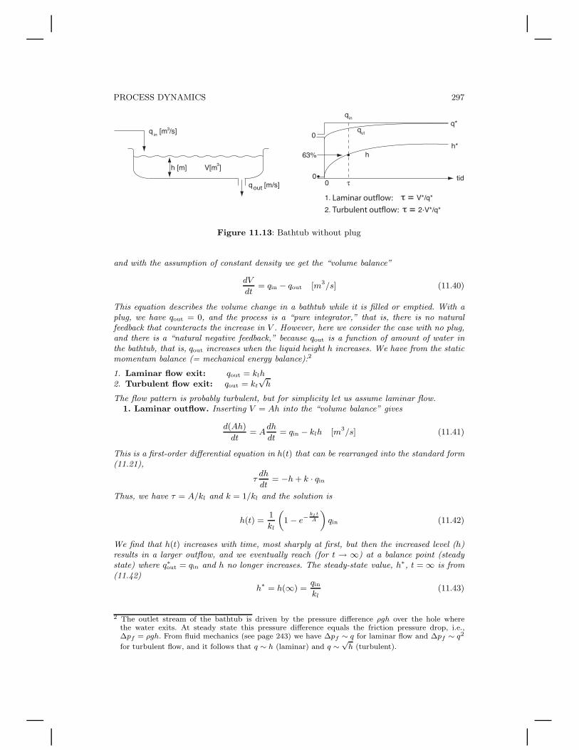
Example 11.9 Mass balance for filling a bathtub without plug. Here, we considerthe dynamics for the volume (level) in a bathtub with no plug, see Figure 11.13. The modelcan also describe the dynamics of the outflow for a tank or the change in the water level in alake following a rainfall. We consider a rectangular bathtub with liquid volume V = Ah whereA [m2] is the base of the tub and h [m] is the liquid height. We assume that the density ρ isconstant.
The control volume (boundary) for the system is the whole bathtub, and the inventory ofmass is m = ρV [kg]. Mass is a conserved quantity, and from (11.3) we get that
dm
dt= win − wout [kg/s] (11.39)
1 For more details on this, and in general on modeling and balance equations, see: R.B. Bird, W.E.Stewart and E.N. Lightfoot, Transport Phenomena, Wiley, 1960.
PROCESS DYNAMICS 297
.
τ
Laminar outflow:
Turbulent outflow:
out
Figure 11.13: Bathtub without plug
and with the assumption of constant density we get the “volume balance”
dV
dt= qin − qout [m3/s] (11.40)
This equation describes the volume change in a bathtub while it is filled or emptied. With aplug, we have qout = 0, and the process is a “pure integrator,” that is, there is no naturalfeedback that counteracts the increase in V . However, here we consider the case with no plug,and there is a “natural negative feedback,” because qout is a function of amount of water inthe bathtub, that is, qout increases when the liquid height h increases. We have from the staticmomentum balance (= mechanical energy balance):2
1. Laminar flow exit: qout = klh2. Turbulent flow exit: qout = kt
√h
The flow pattern is probably turbulent, but for simplicity let us assume laminar flow.1. Laminar outflow. Inserting V = Ah into the “volume balance” gives
d(Ah)
dt= A
dh
dt= qin − klh [m3/s] (11.41)
This is a first-order differential equation in h(t) that can be rearranged into the standard form(11.21),
τdh
dt= −h + k · qin
Thus, we have τ = A/kl and k = 1/kl and the solution is
h(t) =1
kl
„
1 − e−klt
A
«
qin (11.42)
We find that h(t) increases with time, most sharply at first, but then the increased level (h)results in a larger outflow, and we eventually reach (for t → ∞) at a balance point (steadystate) where q∗out = qin and h no longer increases. The steady-state value, h∗, t = ∞ is from(11.42)
h∗ = h(∞) =qin
kl(11.43)
2 The outlet stream of the bathtub is driven by the pressure difference ρgh over the hole wherethe water exits. At steady state this pressure difference equals the friction pressure drop, i.e.,∆pf = ρgh. From fluid mechanics (see page 243) we have ∆pf ∼ q for laminar flow and ∆pf ∼ q2
for turbulent flow, and it follows that q ∼ h (laminar) and q ∼√
h (turbulent).

298 CHEMICAL AND ENERGY PROCESS ENGINEERING
• We can alternatively derive (11.43) from the steady state mass balance, qin = qout [m3/s].Here, qout = klh and (11.43) follows.
• The time constant is τ = A/kl. Here, the steady-state flow rate is q∗ = klh∗(= q∗out = q∗in),
that is, kl = q∗/h∗, and it follows that
τ =A
kl=
Ah∗
q∗=
V ∗
q∗
which equals the residence time of the bathtub. However, so that you won’t think that thetime constant always equals the residence time, please note that for turbulent outflow thetime constant is twice the residence time; this is shown on page 302.
The following example illustrates that the dynamics of gas systems are usually veryfast. This is primarily because of a short residence time, but it is usually furtheramplified by small relative pressure differences.
Example 11.10 Gas dynamics. A large gas tank is used to dampen flow rate and pressurevariations. Derive the dynamic equations and determine the time constant for the pressuredynamics. We assume for simplicity that the inlet and outlet flow rates of the tank are givenby Fin = c1(pin − p) [mol/s] and Fout = c2(p − pout) [mol/s] where the “valve constants” c1
and c2 are assumed to be equal (c1 = c2 = c).
out
outresidence time outin
Figure 11.14: Gas dynamics
Solution. The mass balance is
dn
dt= Fin − Fout [mol/s]
We assume constant volume V and ideal gas,
n =pV
RT
The mass balance then gives:
V
RT
dp
dt= c(pin − p) − c(p − pout)
This equation can be used to compute p as a function of pin, pout and time. Rearranged intostandard form (11.21), we see that the time constant is
τ =V
2cRT=
n
2cp(11.44)
From the steady-state mass balance we get p∗ = (p∗in + p∗
out)/2, so at steady state
F ∗ = F ∗in = F ∗
out = c · p∗in − p∗
out
2
Substituting the resulting value for c into (11.44) gives
τ =n∗
2cp∗=
1
4· n∗
F ∗· p∗
in − p∗out
p∗(11.45)
PROCESS DYNAMICS 299
that is, the time constant is 1/4 of the residence time, n/F , multiplied by the relative pressuredifference, (pin − pout)/p. For gas systems, both these terms are usually small, which explainswhy the pressure dynamics are usually very fast.
For example, with p∗in = 10.1 bar, p∗ = 10 bar and p∗
out = 9.9 bar we get
τ =1
4· n∗
F ∗· 10.1 − 9.9
10=
1
4· 1
50· n∗
F ∗
that is, the time constant for the pressure dynamics in the tank is only 1/200 of the (alreadysmall) residence time.
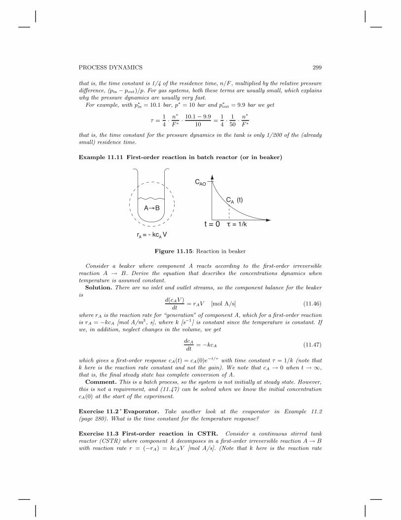
Example 11.11 First-order reaction in batch reactor (or in beaker)
Figure 11.15: Reaction in beaker
Consider a beaker where component A reacts according to the first-order irreversiblereaction A → B. Derive the equation that describes the concentrations dynamics whentemperature is assumed constant.
Solution. There are no inlet and outlet streams, so the component balance for the beakeris
d(cAV )
dt= rAV [mol A/s] (11.46)
where rA is the reaction rate for “generation” of component A, which for a first-order reactionis rA = −kcA [mol A/m3, s], where k [s−1] is constant since the temperature is constant. Ifwe, in addition, neglect changes in the volume, we get
dcA
dt= −kcA (11.47)
which gives a first-order response cA(t) = cA(0)e−t/τ with time constant τ = 1/k (note thatk here is the reaction rate constant and not the gain). We note that cA → 0 when t → ∞,that is, the final steady state has complete conversion of A.
Comment. This is a batch process, so the system is not initially at steady state. However,this is not a requirement, and (11.47) can be solved when we know the initial concentrationcA(0) at the start of the experiment.
Exercise 11.2 ∗ Evaporator. Take another look at the evaporator in Example 11.2(page 280). What is the time constant for the temperature response?
Exercise 11.3 First-order reaction in CSTR. Consider a continuous stirred tankreactor (CSTR) where component A decomposes in a first-order irreversible reaction A → Bwith reaction rate r = (−rA) = kcAV [mol A/s]. (Note that k here is the reaction rate

300 CHEMICAL AND ENERGY PROCESS ENGINEERING
constant and not the process gain). The feed concentration is cA,F . Derive the equation thatdescribes the concentration dynamics when temperature is assumed constant. Find the timeconstant and gain for the response.
11.3.4 Time response for more complex systems
In the previous section, we considered in detail the step response for systems withonly one differential equation which can be written in “standard” form τdy(t)/dt =−y(t) + k u(t). This gave rise to a first-order response. Although many systems canbe written (or approximated) by a first-order response, it must be emphasized thatthe responses are generally far more complex.
time
Tin ToutTout
Tin
T
Tin
Figure 11.16: Temperature response for stirred tank with bypass
• Even for systems with only one linear differential equation, the response can bedifferent from that described above, either because the system is non-linear orbecause the response has a “direct term,” that is, the equation can be writtenin the form
τdx(t)/dt = −x(t) + ku(t); y(t) = c · x(t) + d · u(t)
where the d 6= 0 gives a “direct term” from u to y (see for example Figure 11.16which shows the response of a stirred tank with bypass).
• If we have two first-order systems in series, for example two stirred tanks, thetotal response will be second-order, and if we have n first-order systems in a series,the total response is nth-order. The response for such higher-order systems willusually have a “flatter” initial response (see Figure 11.22, page 309), and is oftenapproximated as an effective time delay.
• We will also have a higher-order response if the model consists of several coupleddifferential equations, for example, an adiabatic reactor with coupled material andenergy balance (see Figure 11.24, page 312).
The analytic expression for the time response of higher-order system is usuallyrather complicated, and often there is no analytical solution. However, by linearizingthe system, as discussed in the next section (Section 11.4), it is possible to use effectivemathematical tools for analyzing the system, for example, by computing the system’s“poles” (=eigenvalues = −1/time constant) and “zeros.” The most important toolfor analyzing more complex systems is nevertheless “dynamic simulation,” that is,numerical solution of the equations. This is discussed in Section 11.5.
PROCESS DYNAMICS 301
Exercise 11.4 (a) Derive the model for the stirred tank with bypass shown in Figure 11.16and (b) find an analytical expression for the time response.
11.4 Linearization
Consider a dynamic modeldy
dt= f(y, u) (11.48)
This model is linear if the function f(y, u) is linear, which means that if we doublethe change in u (or in y) then the change in f is doubled. In general our models arenonlinear, but we are often interested in studying the response of small changes in u,and we can then use a linearized model. The most important use of linearized modelsis in control engineering, where the objective of the control is indeed to keep y closeto its desired value (that is, ∆y is indeed small) such that the assumption of linearmodel often holds well.
Let y∗ and u∗ denote the values of y and u at the operating point ∗ (or along thenominal trajectory y∗(t)) where we linearize the model. This is often a steady-statepoint but does not need to be. A first-order Taylor-series expansion (“tangentapproximation”) of the function f(y, u), where we neglect the second-order (with∆u2, ∆y2, ∆u∆y) and higher-order terms, gives a linearized approximation
f(y, u) ≈ f(y∗, u∗)︸ ︷︷ ︸
f∗
+
(∂f
∂u
)∗
∆u +
(∂f
∂y
)∗
∆y
︸ ︷︷ ︸
∆f
(11.49)
where ∆u = u − u∗ and ∆y = y − y∗ represent the deviations from the nominaloperating point. The approximation is exact for small values of ∆u and ∆y. Further,we have that
d∆y
dt=
d(y − y∗)
dt=
dy
dt− dy∗
dt︸︷︷︸
f∗
For the non-linear model (11.48) we have then derived a linearized model indeviation variables,
d∆y
dt= ∆f =
(∂f
∂y
)∗
︸ ︷︷ ︸
a
∆y +
(∂f
∂u
)∗
︸ ︷︷ ︸
b
∆u (11.50)
where the coefficients a and b denote the local derivatives with respect to y and u,respectively. Comparing this with the standard form for first-order systems in (11.21),
τd∆y
dt= −∆y + k∆u
we find
τ = −1
a; k = − b
aThus, linearized models can be used to determine the time constant τ .
302 CHEMICAL AND ENERGY PROCESS ENGINEERING
Example 11.12 Linearized model for turbulent outflow of tank. This is acontinuation of Example 11.9 (page 296) where we considered laminar outflow of a bathtub.For case 2 with turbulent outflow, qout = kt
√h, the “volume balance” (11.41) for filling the
bathtub becomes
Adh
dt= qin − kt
√h = f(h, qin) [m3/s] (11.51)
Here, the function f is non-linear in h. Linearizing f and introducing deviation variablesgives, see (11.50),
Ad∆h
dt= ∆f = ∆qin − kt
1
2√
h∗∆h
Comparison with the standard form with y = ∆h and u = ∆qin gives τ = 2√
h∗A/kt, where
from (11.51), kt = q∗/√
h∗ and q∗ is the steady state flow. Further rearrangement of theexpression for the time constant gives
τ = 2
√h∗A
kt= 2
h∗A
q∗= 2 · V ∗
q∗
That is, the time constant is two times the residence time (while it was equal to the residencetime with laminar outflow). In other words, we can, by comparing the experimental timeconstant with the residence time, predict whether the outflow is laminar or turbulent. Alsonote that the steady state gain k = ∆h(∞)/∆qin = 2h∗/q∗ for turbulent flow is twice that oflaminar flow.
Comment. Note that the initial response for h(t) (expressed by the slope k′ = k/τ) isthe same for both cases, k′ = k/τ = 1/A. This is reasonable since the outlet flow (wherethe difference between turbulent and laminar flow lies) is only affected after the level startschanging.
or
Turbulent or laminar?
Figure 11.17: Student anxious to check the outflow from a sink
Exercise 11.5 Experiment at home. You should check whether the outflow from yoursink is laminar or turbulent by comparing the time constant τ of the dynamic response insink level with the residence (holdup) time τh = V/q:
1. With the plug out, adjust the inflow such that the level is at a steady state where the sinkis a little more than half full.
2. Reduce the inflow and record the level response (use a ruler and read off the level at regularintervals). From this experiment estimate the time constant τ (when 63% of the steady-state change is reached). This assumes that the area A is reasonably constant in the regionbetween the two steady-state levels.
PROCESS DYNAMICS 303
3. Temporarily lead the water somewhere else (but keep the same flow), for example, into abucket, such that the sink is emptied. Put in the plug and let again the water flow into thesink. Measure the time it takes to fill the tank to its previous level. This is the residencetime τh = V/q.
4. If τ ≈ τh, the outflow is laminar, and if τ ≈ 2τh, it is turbulent. (Note that it is possible,but not very likely, that you get a transition from turbulent to laminar flow when q isreduced).
5. Another way of checking whether the flow is laminar or turbulent is to find the residencetime τh for two different steady state levels (see point 3); if the flow is laminar, thenτh = A/kl is independent (!) of the level h, but if the flow is turbulent, then τh =
√hA/kt
increases with the square root of the level.
Multivariable and higher-order systems. We have above assumed that we havea scalar model with one input variable u and one output variable y. It is, however,easy to generalize the linearization to the multi-dimensional case where the coefficients(derivatives) A = ∂f/∂y and B = ∂f/∂u become matrices. The model in deviationvariables is then
d∆y
dt= A∆y + B∆u
∆u: vector of independent variables (inputs or disturbances)
∆y: vector of dependent state variables (often denoted x)
(Note that we, for simplicity, have not introduced separate symbols for vectors, butwe could for clarity have written u and y).
The concept of time constant is less clear in the multivariable case, but we caninstead compute the eigenvalues λi of the matrix A:
• We find that the “time constants” τi = −1/λi(A) appear in the linearized timeresponse which contains the term e−t/τi . For the scalar case with only one equation(A = a = scalar), the eigenvalue of A equals a, and we find τ = −1/a.
• The system is (locally) stable if and only if all eigenvalues of A have a negative realpart (i.e., the eigenvalues are in the left-half complex plane).
11.5 Dynamic simulation with examples
By the expression “dynamic simulation,” we mean “numerical solution (integration)of the system’s differential equations as a function of time.”
We consider a dynamic system described by the differential equations
dy
dt= f(y, u)
where
1. The initial state y(t0) = y0 is known (we need one for every differential equation).2. The independent variables u(t) are known for t > t0.
304 CHEMICAL AND ENERGY PROCESS ENGINEERING
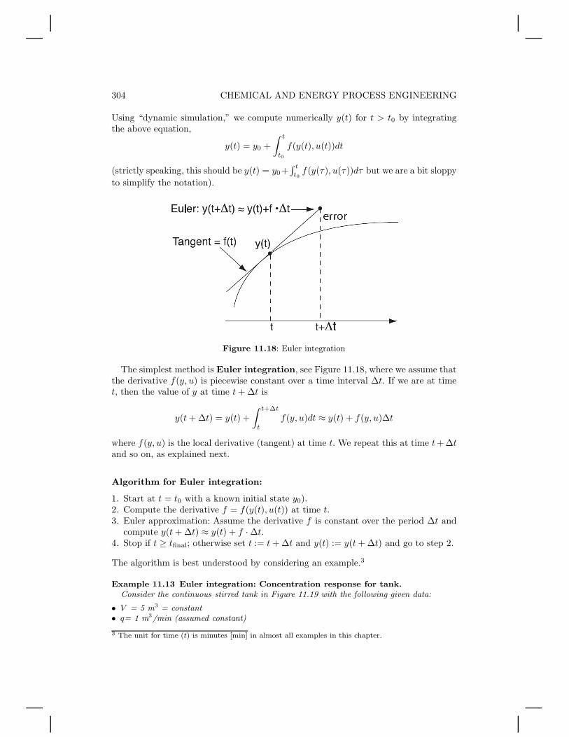
Using “dynamic simulation,” we compute numerically y(t) for t > t0 by integratingthe above equation,
y(t) = y0 +
∫ t
t0
f(y(t), u(t))dt
(strictly speaking, this should be y(t) = y0+∫ t
t0f(y(τ), u(τ))dτ but we are a bit sloppy
to simplify the notation).
Figure 11.18: Euler integration
The simplest method is Euler integration, see Figure 11.18, where we assume thatthe derivative f(y, u) is piecewise constant over a time interval ∆t. If we are at timet, then the value of y at time t + ∆t is
y(t + ∆t) = y(t) +
∫ t+∆t
t
f(y, u)dt ≈ y(t) + f(y, u)∆t
where f(y, u) is the local derivative (tangent) at time t. We repeat this at time t + ∆tand so on, as explained next.
Algorithm for Euler integration:
1. Start at t = t0 with a known initial state y0).2. Compute the derivative f = f(y(t), u(t)) at time t.3. Euler approximation: Assume the derivative f is constant over the period ∆t and
compute y(t + ∆t) ≈ y(t) + f · ∆t.4. Stop if t ≥ tfinal; otherwise set t := t + ∆t and y(t) := y(t + ∆t) and go to step 2.
The algorithm is best understood by considering an example.3
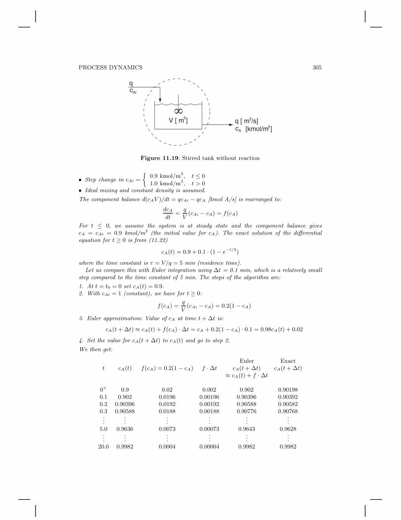
Example 11.13 Euler integration: Concentration response for tank.Consider the continuous stirred tank in Figure 11.19 with the following given data:
• V = 5 m3 = constant• q= 1 m3/min (assumed constant)
3 The unit for time (t) is minutes [min] in almost all examples in this chapter.
PROCESS DYNAMICS 305
Figure 11.19: Stirred tank without reaction
• Step change in cAi =
0.9 kmol/m3, t ≤ 0
1.0 kmol/m3, t > 0• Ideal mixing and constant density is assumed.
The component balance d(cAV )/dt = qcAi − qcA [kmol A/s] is rearranged to:
dcA
dt=
q
V(cAi − cA) = f(cA)
For t ≤ 0, we assume the system is at steady state and the component balance givescA = cAi = 0.9 kmol/m3 (the initial value for cA). The exact solution of the differentialequation for t ≥ 0 is from (11.22)
cA(t) = 0.9 + 0.1 · (1 − e−t/5)
where the time constant is τ = V/q = 5 min (residence time).Let us compare this with Euler integration using ∆t = 0.1 min, which is a relatively small
step compared to the time constant of 5 min. The steps of the algorithm are:
1. At t = t0 = 0 set cA(t) = 0.9.2. With cAi = 1 (constant), we have for t ≥ 0:
f(cA) =q
V(cAi − cA) = 0.2(1 − cA)
3. Euler approximation: Value of cA at time t + ∆t is:
cA(t + ∆t) ≈ cA(t) + f(cA) · ∆t = cA + 0.2(1 − cA) · 0.1 = 0.98cA(t) + 0.02
4. Set the value for cA(t + ∆t) to cA(t) and go to step 2.
We then get:
Euler Exactt cA(t) f(cA) = 0.2(1 − cA) f · ∆t cA(t + ∆t) cA(t + ∆t)
≈ cA(t) + f · ∆t
0+ 0.9 0.02 0.002 0.902 0.901980.1 0.902 0.0196 0.00196 0.90396 0.903920.2 0.90396 0.0192 0.00192 0.90588 0.905820.3 0.90588 0.0188 0.00188 0.90776 0.90768...
......
......
...5.0 0.9636 0.0073 0.00073 0.9643 0.9628...
......
......
...20.0 0.9982 0.0004 0.00004 0.9982 0.9982
306 CHEMICAL AND ENERGY PROCESS ENGINEERING
We see, as expected, that Euler integration gives a numerical error; see alsoFigure 11.20. This error can be reduced by reducing the step length ∆t, but thisincreases the computational effort and if it becomes too small it may conflict withthe accuracy of the computer. On the other hand, if ∆t gets too large, the Eulerintegration may go unstable.
There are many possible improvements to Euler integration
• Higher-order method: Include more terms in the Taylor-series expansion for y (Eulerassumes y ≈ y0 + f∆t).
• Introduce step length control (adjusting ∆t during integration).• Use an implicit solution that avoids the possible instability, for example, implicit
Euler:y(t + ∆t) ≈ y(t) + f (y(t + ∆t), u(t + ∆t)) · ∆t
which has to be solved with respect to y(t + ∆t).
Examples of MATLAB routines which include improvements of this kind are ode45
and ode15s (the latter is recommended for most problems).
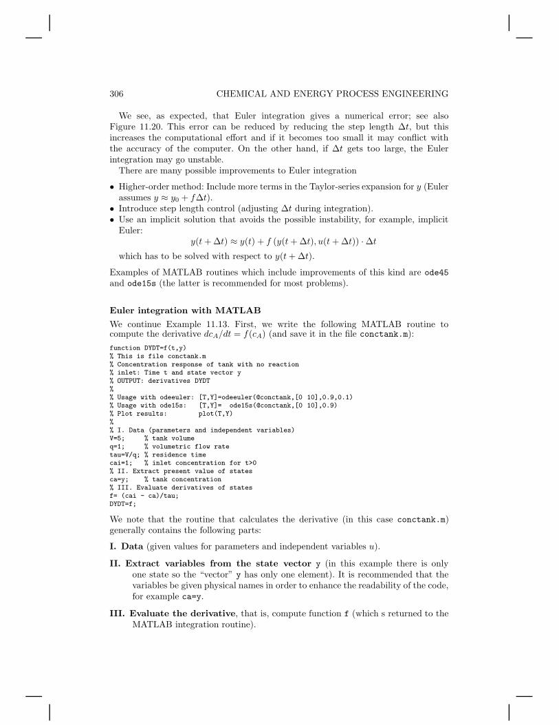
Euler integration with MATLAB
We continue Example 11.13. First, we write the following MATLAB routine tocompute the derivative dcA/dt = f(cA) (and save it in the file conctank.m):
function DYDT=f(t,y)% This is file conctank.m% Concentration response of tank with no reaction% inlet: Time t and state vector y% OUTPUT: derivatives DYDT%% Usage with odeeuler: [T,Y]=odeeuler(@conctank,[0 10],0.9,0.1)% Usage with ode15s: [T,Y]= ode15s(@conctank,[0 10],0.9)% Plot results: plot(T,Y)%% I. Data (parameters and independent variables)V=5; % tank volumeq=1; % volumetric flow ratetau=V/q; % residence timecai=1; % inlet concentration for t>0% II. Extract present value of statesca=y; % tank concentration% III. Evaluate derivatives of statesf= (cai - ca)/tau;DYDT=f;
We note that the routine that calculates the derivative (in this case conctank.m)generally contains the following parts:
I. Data (given values for parameters and independent variables u).
II. Extract variables from the state vector y (in this example there is onlyone state so the “vector” y has only one element). It is recommended that thevariables be given physical names in order to enhance the readability of the code,for example ca=y.
III. Evaluate the derivative, that is, compute function f (which s returned to theMATLAB integration routine).

PROCESS DYNAMICS 307
In addition, we need a program that computes the numerical solution (“performsthe integration”). Below is a simple program for Euler integration which is savedin the file odeeuler.m:
function [tout,yout]=odeeuler(odefile,tspan,y0,H)% This is the function odeeuler.m% Simple integration routine written by SiS in 1998% Usage: [T,Y]=odeeuler(@F,TSPAN,Y0,H)% for example: [T,Y]=odeeuler(@conctank,[0 10],0.9,0.1)%% T - solution time vector.% Y - solution state (output) vector.% F - filename with diff.eqns. (see also help ode15s).% TSPAN = [initial_time final_time}% Y0 - initial state vector% H - integration step size%t0=tspan(1); tfinal=tspan(2);% Initializetout=t0; yout=y0; neq=length(y0); t=t0; y=y0;% Integratewhile t < tfinal,t=t+H;f=feval(odefile,t,y);
for i=1:neq,y(i)=y(i)+H*f(i);end
tout=[tout;t]; yout=[yout; y];end
We can now use MATLAB to compute the concentration response using Eulerintegration:
>> [T,Y]=odeeuler(@conctank,[0 1],0.9,0.1)
T =0
0.10000.20000.30000.40000.50000.60000.70000.80000.90001.00001.1000
Y =0.90000.90200.90400.90590.90780.90960.91140.91320.91490.91660.91830.9199
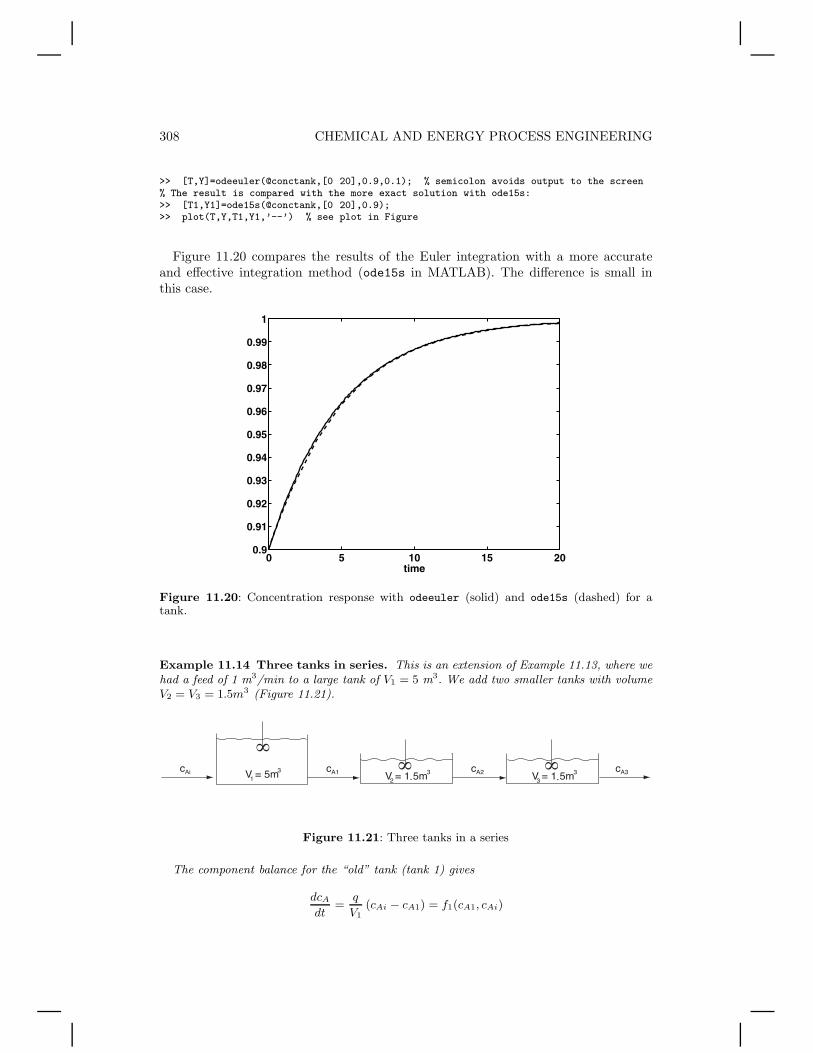
308 CHEMICAL AND ENERGY PROCESS ENGINEERING
>> [T,Y]=odeeuler(@conctank,[0 20],0.9,0.1); % semicolon avoids output to the screen% The result is compared with the more exact solution with ode15s:>> [T1,Y1]=ode15s(@conctank,[0 20],0.9);>> plot(T,Y,T1,Y1,’--’) % see plot in Figure
Figure 11.20 compares the results of the Euler integration with a more accurateand effective integration method (ode15s in MATLAB). The difference is small inthis case.
0 5 10 15 200.9
0.91
0.92
0.93
0.94
0.95
0.96
0.97
0.98
0.99
1
time0 5 10 15 20
0.9
0.91
0.92
0.93
0.94
0.95
0.96
0.97
0.98
0.99
1
time
Figure 11.20: Concentration response with odeeuler (solid) and ode15s (dashed) for atank.
Example 11.14 Three tanks in series. This is an extension of Example 11.13, where wehad a feed of 1 m3/min to a large tank of V1 = 5 m3. We add two smaller tanks with volumeV2 = V3 = 1.5m3 (Figure 11.21).
Figure 11.21: Three tanks in a series
The component balance for the “old” tank (tank 1) gives
dcA
dt=
q
V1(cAi − cA1) = f1(cA1, cAi)
PROCESS DYNAMICS 309
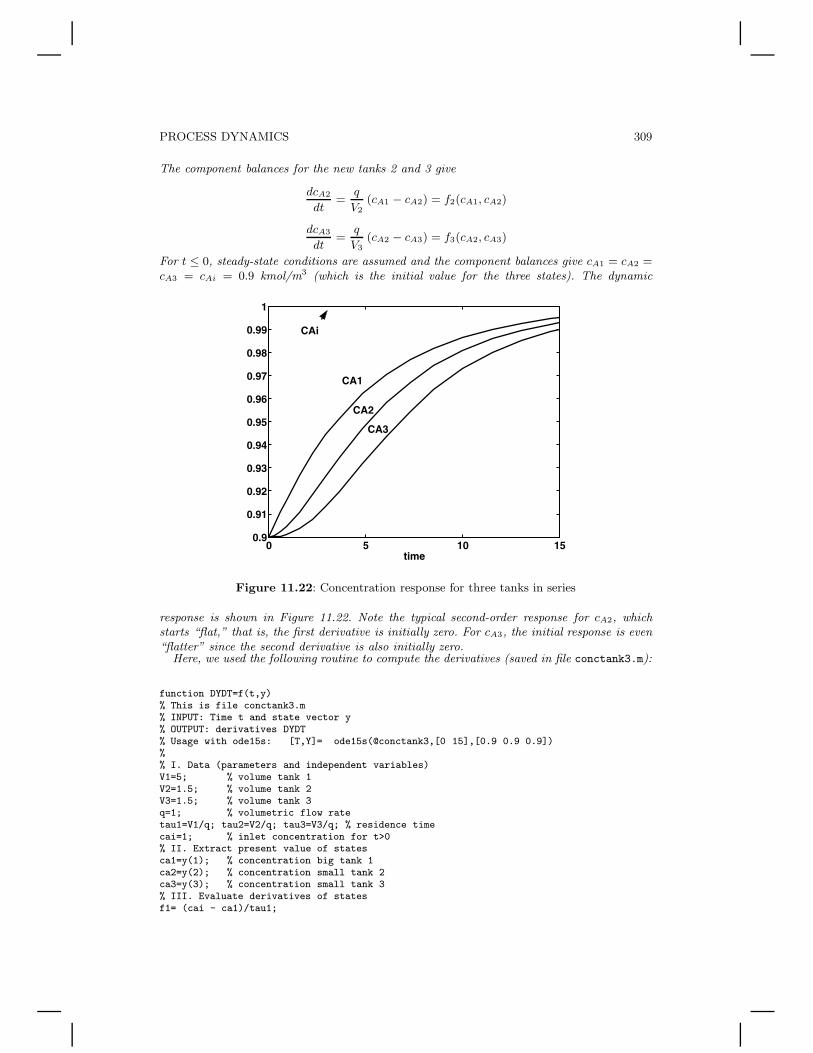
The component balances for the new tanks 2 and 3 give
dcA2
dt=
q
V2(cA1 − cA2) = f2(cA1, cA2)
dcA3
dt=
q
V3(cA2 − cA3) = f3(cA2, cA3)
For t ≤ 0, steady-state conditions are assumed and the component balances give cA1 = cA2 =cA3 = cAi = 0.9 kmol/m3 (which is the initial value for the three states). The dynamic
0 5 10 150.9
0.91
0.92
0.93
0.94
0.95
0.96
0.97
0.98
0.99
1
time
CAi
CA1
CA2
CA3
0 5 10 150.9
0.91
0.92
0.93
0.94
0.95
0.96
0.97
0.98
0.99
1
time
CAi
CA1
CA2
CA3
Figure 11.22: Concentration response for three tanks in series
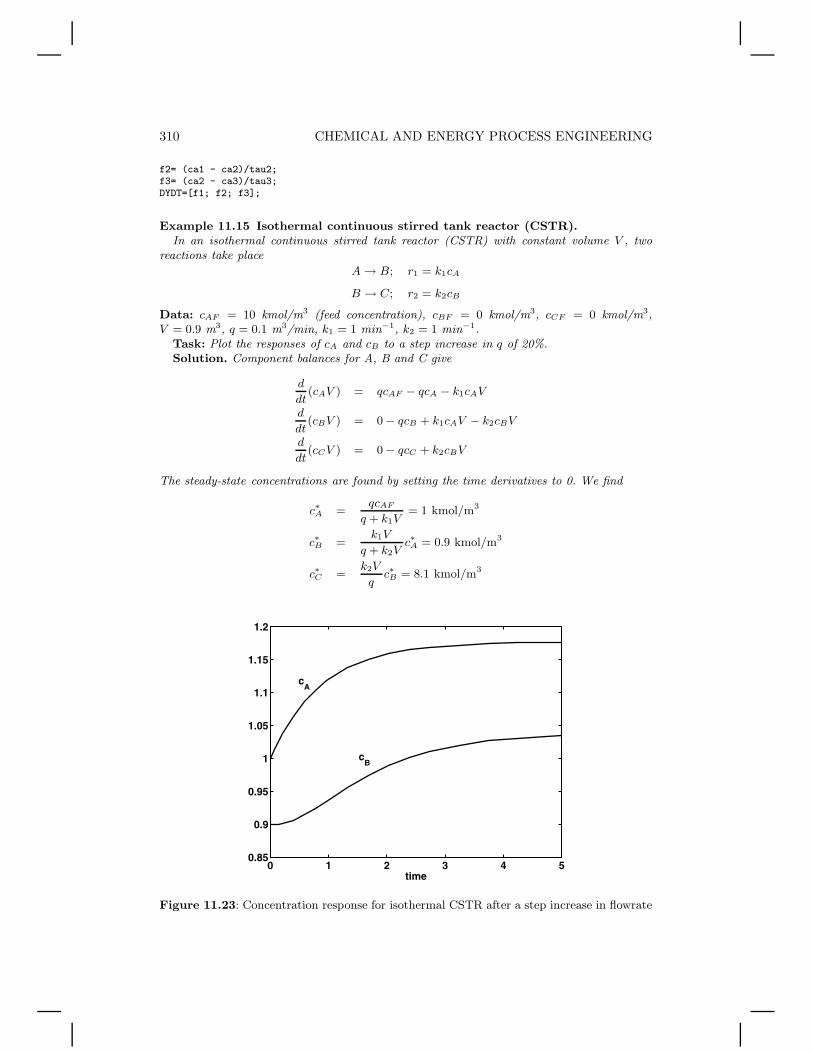
response is shown in Figure 11.22. Note the typical second-order response for cA2, whichstarts “flat,” that is, the first derivative is initially zero. For cA3, the initial response is even“flatter” since the second derivative is also initially zero.
Here, we used the following routine to compute the derivatives (saved in file conctank3.m):
function DYDT=f(t,y)% This is file conctank3.m% INPUT: Time t and state vector y% OUTPUT: derivatives DYDT% Usage with ode15s: [T,Y]= ode15s(@conctank3,[0 15],[0.9 0.9 0.9])%% I. Data (parameters and independent variables)V1=5; % volume tank 1V2=1.5; % volume tank 2V3=1.5; % volume tank 3q=1; % volumetric flow ratetau1=V1/q; tau2=V2/q; tau3=V3/q; % residence timecai=1; % inlet concentration for t>0% II. Extract present value of statesca1=y(1); % concentration big tank 1ca2=y(2); % concentration small tank 2ca3=y(3); % concentration small tank 3% III. Evaluate derivatives of statesf1= (cai - ca1)/tau1;
310 CHEMICAL AND ENERGY PROCESS ENGINEERING
f2= (ca1 - ca2)/tau2;f3= (ca2 - ca3)/tau3;DYDT=[f1; f2; f3];
Example 11.15 Isothermal continuous stirred tank reactor (CSTR).In an isothermal continuous stirred tank reactor (CSTR) with constant volume V , two
reactions take place
A → B; r1 = k1cA
B → C; r2 = k2cB
Data: cAF = 10 kmol/m3 (feed concentration), cBF = 0 kmol/m3, cCF = 0 kmol/m3,V = 0.9 m3, q = 0.1 m3/min, k1 = 1 min−1, k2 = 1 min−1.
Task: Plot the responses of cA and cB to a step increase in q of 20%.Solution. Component balances for A, B and C give
d
dt(cAV ) = qcAF − qcA − k1cAV
d
dt(cBV ) = 0 − qcB + k1cAV − k2cBV
d
dt(cCV ) = 0 − qcC + k2cBV
The steady-state concentrations are found by setting the time derivatives to 0. We find
c∗A =qcAF
q + k1V= 1 kmol/m3
c∗B =k1V
q + k2Vc∗A = 0.9 kmol/m3
c∗C =k2V
qc∗B = 8.1 kmol/m3
0 1 2 3 4 50.85
0.9
0.95
1
1.05
1.1
1.15
1.2
time
cA
cB
0 1 2 3 4 50.85
0.9
0.95
1
1.05
1.1
1.15
1.2
time
cA
cB
Figure 11.23: Concentration response for isothermal CSTR after a step increase in flowrate
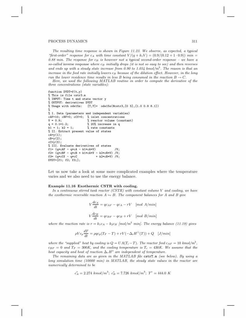
PROCESS DYNAMICS 311
The resulting time response is shown in Figure 11.23. We observe, as expected, a typical“first-order” response for cA with time constant V/(q + k1V ) = (0.9/(0.12 + 1 · 0.9)) min =0.88 min. The response for cB is however not a typical second-order response – we have aso-called inverse response where cB initially drops (it is not so easy to see) and then reversesand ends up with a steady state increase from 0.90 to 1.034 kmol/m3. The reason is that anincrease in the feed rate initially lowers cB because of the dilution effect. However, in the longrun the lower residence time results in less B being consumed in the reaction B → C.
Here, we used the following MATLAB routine in order to compute the derivative of thethree concentrations (state variables):
function DYDT=f(t,y)% This is file cstr3.m% INPUT: Time t and state vector y% OUTPUT: derivatives DYDT% Usage with ode15s: [T,Y]= ode15s(@cstr3,[0 5],[1.0 0.9 8.1])%% I. Data (parameters and independent variables)cAF=10; cBF=0; cCf=0; % inlet concentrationsV = 0.9; % reactor volume (constant)q = 0.1*1.2; % 20% increase in qk1 = 1; k2 = 1; % rate constants% II. Extract present value of statescA=y(1);cB=y(2);cC=y(3);% III. Evaluate derivatives of statesf1= (q*cAF - q*cA - k1*cA*V) /V;f2= (q*cBF - q*cB + k1*cA*V - k2*cB*V) /V;f3= (q*cCf - q*cC + k2*cB*V) /V;DYDT=[f1; f2; f3;];
Let us now take a look at some more complicated examples where the temperaturevaries and we also need to use the energy balance.
Example 11.16 Exothermic CSTR with cooling.In a continuous stirred tank reactor (CSTR) with constant volume V and cooling, we have
the exothermic reversible reaction A ⇌ B. The component balances for A and B give
VdcA
dt= qcAF − qcA − rV [mol A/min]
VdcB
dt= qcBF − qcB + rV [mol B/min]
where the reaction rate is r = k1cA − k2cB [mol/m3 min]. The energy balance (11.19) gives
ρV cpdT
dt= ρqcp(TF − T ) + rV (−∆rH
⊖(T )) + Q [J/min]
where the “supplied” heat by cooling is Q = UA(Tc−T ). The reactor feed cAF = 10 kmol/m3,cBF = 0 and TF = 300K, and the cooling temperature is Tc = 430K. We assume that theheat capacity and heat of reaction ∆rH
o are independent of temperature.The remaining data are as given in the MATLAB file cstrT.m (see below). By using a
long simulation time (10000 min) in MATLAB, the steady state values in the reactor arenumerically determined to be
c∗A = 2.274 kmol/m3; c∗B = 7.726 kmol/m3; T ∗ = 444.0 K
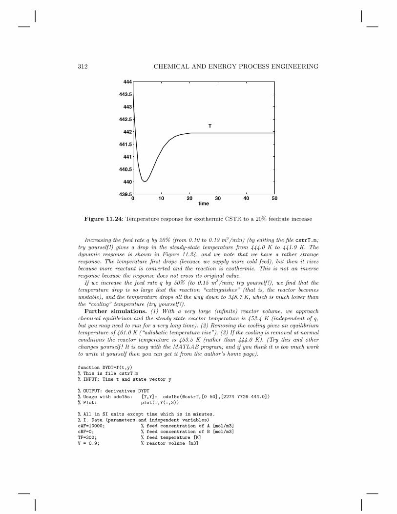
312 CHEMICAL AND ENERGY PROCESS ENGINEERING
0 10 20 30 40 50439.5
440
440.5
441
441.5
442
442.5
443
443.5
444
time
T
0 10 20 30 40 50439.5
440
440.5
441
441.5
442
442.5
443
443.5
444
time
T
Figure 11.24: Temperature response for exothermic CSTR to a 20% feedrate increase
Increasing the feed rate q by 20% (from 0.10 to 0.12 m3/min) (by editing the file cstrT.m;try yourself !) gives a drop in the steady-state temperature from 444.0 K to 441.9 K. Thedynamic response is shown in Figure 11.24, and we note that we have a rather strangeresponse. The temperature first drops (because we supply more cold feed), but then it risesbecause more reactant is converted and the reaction is exothermic. This is not an inverseresponse because the response does not cross its original value.
If we increase the feed rate q by 50% (to 0.15 m3/min; try yourself !), we find that thetemperature drop is so large that the reaction “extinguishes” (that is, the reactor becomesunstable), and the temperature drops all the way down to 348.7 K, which is much lower thanthe “cooling” temperature (try yourself !).
Further simulations. (1) With a very large (infinite) reactor volume, we approachchemical equilibrium and the steady-state reactor temperature is 453.4 K (independent of q,but you may need to run for a very long time). (2) Removing the cooling gives an equilibriumtemperature of 461.0 K (“adiabatic temperature rise”). (3) If the cooling is removed at normalconditions the reactor temperature is 453.5 K (rather than 444.0 K). (Try this and otherchanges yourself ! It is easy with the MATLAB program; and if you think it is too much workto write it yourself then you can get it from the author’s home page).
function DYDT=f(t,y)% This is file cstrT.m% INPUT: Time t and state vector y
% OUTPUT: derivatives DYDT% Usage with ode15s: [T,Y]= ode15s(@cstrT,[0 50],[2274 7726 444.0])% Plot: plot(T,Y(:,3))
% All in SI units except time which is in minutes.% I. Data (parameters and independent variables)cAF=10000; % feed concentration of A [mol/m3]cBF=0; % feed concentration of B [mol/m3]TF=300; % feed temperature [K]V = 0.9; % reactor volume [m3]

PROCESS DYNAMICS 313
q = 0.10; % volumetric flow rate [m3/min] (CAN CHANGE, e.g., to 0.12)dhr= -80e3; % Heat of reaction [J/mol]cp= 4.e3; % specific heat capacity [J/kg K]rho = 1000; % mean density [kg/m3]U = 1000*60; % overall heat transfer coefficient [J/min,m2,K]A = 5; % heat transfer area [m2]Tc = 430; % cooling temperature [K]k1_400 = 0.1; % rx1: rate constant at 400K [1/min]k2_400 = 0.001; % rx2: rate constant at 400K [1/min]E1 = 60e3; % rx1: activation energy [J/mol]E2 = E1 - dhr; % rx2: activation energy [J/mol]R = 8.31; % gas constant [J/K mol]% II. Extract present value of statescA=y(1);cB=y(2);T=y(3);% IIIa. Intermediate calculationsk1 = k1_400 * exp(-(E1/R) * (1/T - 1/400));k2 = k2_400 * exp(-(E2/R) * (1/T - 1/400));r = k1*cA - k2*cB;Q = U*A*(Tc-T);% IIIb. Evaluate derivatives of statesVdcadt = q*cAF - q*cA - r*V; % [mol A/min]Vdcbdt = q*cBF - q*cB + r*V; % [mol B/min]mcpdTdt = rho*q*cp*(TF-T) + r*V*(-dhr) + Q; % [J/min]
f1 = Vdcadt/V;f2 = Vdcbdt/V;f3 = mcpdTdt / (rho*cp*V);
DYDT=[f1; f2; f3];
In the above example, we assumed that the heat capacities and the heat of reactionwere independent of temperature. For the more general cases, it is recommended thatthe energy balance is written in its original form with U (or H) as a state, and that T isfound numerically from the implicit algebraic equation U = U0(T, p, ni), as describedfor the flash tank in Example 11.18.
Exercise 11.6 Second-order reaction in CSTR Consider a continuous stirred tankreactor (CSTR) where component A decomposes in a second-order irreversible reaction2A → B with reaction rate r = rB = kc2
AV [kmol/s]. The following steady state data aregiven: V ∗ = 30 m3 (constant), q∗ = 0.5 m3/s, c∗AF = 4 kmol/m3 , c∗BF = 0 kmol/m3 (feed),c∗B = 1 kmol/m3 (product and tank).
(a) Derive the equations that describe the concentration dynamics when the temperatureand volume are assumed constant.
(b) Use the steady state data to determine c∗A and the reaction rate constant k.(c) Linearize the model and determine an expression for the time constant for the
concentration response for component A in the nominal working point.(d) Sketch the expected response cA(t) (in product/tank) when we at t = 0 throw in some
catalyst such that k is doubled. (For calculations by hand you can for example use Eulerintegration of the balance for component A with ∆t = 5 s). What is the new steady statevalue of cA? What is the time constant?
Distillation examples
Example 11.17 Dynamics of distillation column (Figure 11.25). In a distillationcolumn, the components are separated based on their difference in volatility, and multiple
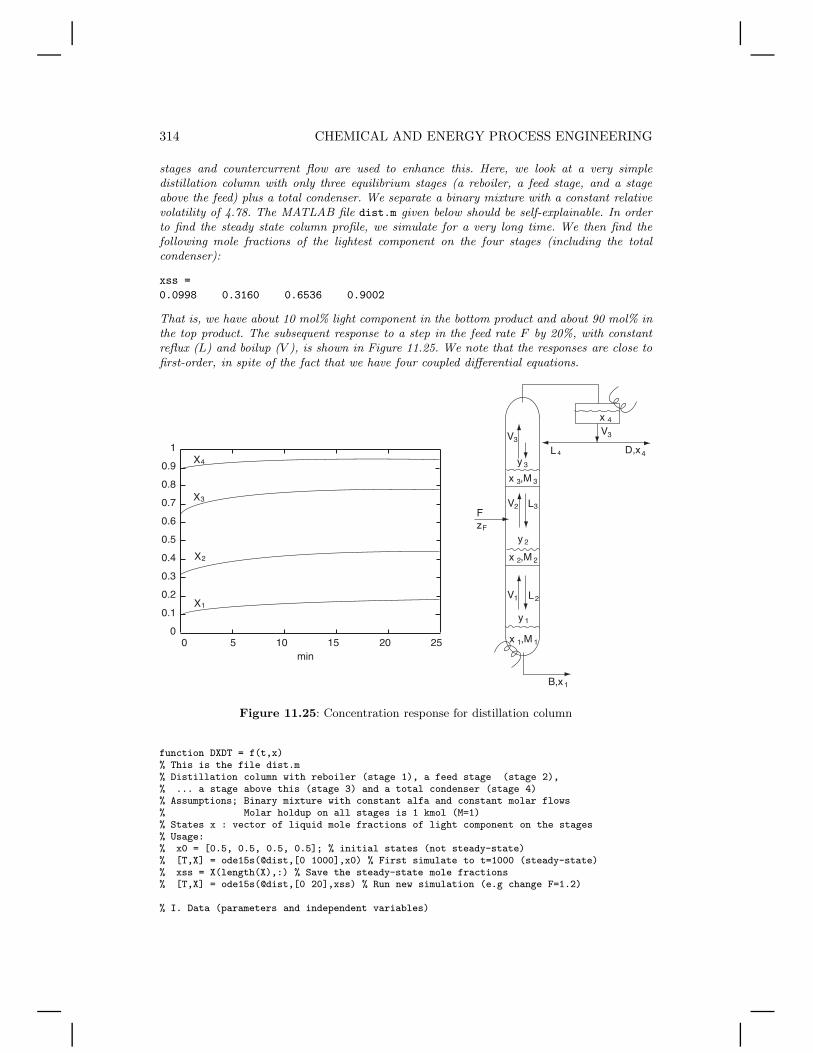
314 CHEMICAL AND ENERGY PROCESS ENGINEERING
stages and countercurrent flow are used to enhance this. Here, we look at a very simpledistillation column with only three equilibrium stages (a reboiler, a feed stage, and a stageabove the feed) plus a total condenser. We separate a binary mixture with a constant relativevolatility of 4.78. The MATLAB file dist.m given below should be self-explainable. In orderto find the steady state column profile, we simulate for a very long time. We then find thefollowing mole fractions of the lightest component on the four stages (including the totalcondenser):
xss =
0.0998 0.3160 0.6536 0.9002
That is, we have about 10 mol% light component in the bottom product and about 90 mol% inthe top product. The subsequent response to a step in the feed rate F by 20%, with constantreflux (L) and boilup (V ), is shown in Figure 11.25. We note that the responses are close tofirst-order, in spite of the fact that we have four coupled differential equations.
Figure 11.25: Concentration response for distillation column
function DXDT = f(t,x)% This is the file dist.m% Distillation column with reboiler (stage 1), a feed stage (stage 2),% ... a stage above this (stage 3) and a total condenser (stage 4)% Assumptions; Binary mixture with constant alfa and constant molar flows% Molar holdup on all stages is 1 kmol (M=1)% States x : vector of liquid mole fractions of light component on the stages% Usage:% x0 = [0.5, 0.5, 0.5, 0.5]; % initial states (not steady-state)% [T,X] = ode15s(@dist,[0 1000],x0) % First simulate to t=1000 (steady-state)% xss = X(length(X),:) % Save the steady-state mole fractions% [T,X] = ode15s(@dist,[0 20],xss) % Run new simulation (e.g change F=1.2)
% I. Data (parameters and independent variables)
PROCESS DYNAMICS 315
% Assume constant relative volatilityalfa = 4.78;
% Feed rate [kmol/min] and feed composition (may change this)F=1.0; zF=0.5;
% Flows in the column [kmol/min] (feed liquid; constant molar flows)V=3.55; V1=V; V2=V; V3=V;L=3.05; L4=L; L3=L; L2=L+F;% Assume constant condenser and reboiler holdup (perfect level control):D=V3-L4; B=L2-V1;
% II. Extract present value of states% ..... Not needed here since x is the state which is already a good name
% IIIa. Intermediate calculations% Vapor-liquid equilibrium (constant relative volatility)y(1) = alfa*x(1)/(1+(alfa-1)*x(1));y(2) = alfa*x(2)/(1+(alfa-1)*x(2));y(3) = alfa*x(3)/(1+(alfa-1)*x(3));y(4)=x(4); % total condenser
% IIIb. Evaluate derivatives of states% Component balances (assume constant stage holdups M1=M2=M3=M4=1 [kmol])DXDT(1) = L2*x(2)-V1*y(1)-B*x(1);DXDT(2) = L3*x(3)+V1*y(1)-L2*x(2)-V2*y(2)+F*zF;DXDT(3) = L4*x(4)+V2*y(2)-L3*x(3)-V3*y(3);DXDT(4) = V3*y(3)-L4*x(4)-D*x(4);
% Change vector DXDT to a column vector (MATLAB requires this..).DXDT=DXDT’;
The above routine does not make use of MATLAB’s vector calculation features.However, below is given an excerpt from a more general routine which uses vectors.Note that we use element-by-element operators *. and ./ to multiply and dividevectors. This code also allows for variable stage holdup M(i), which is important ifthe model is to be used for control purposes. It is simple to change the number ofstages NT in the column.
% From code for general distillation column dynamics% Vapor-liquid equilibriai=1:NT-1; y(i)=alpha*x(i)./(1+(alpha-1)*x(i));
% Need algebraic for computing L(i) (e.g., Francis weir)% and V(i) (e.g., constant molar flows or ‘‘valve" equation)% ..... but these are not given here.
% Column mass balancesi=2:NT-1;dMdt(i) = L(i+1) - L(i) + V(i-1) - V(i);dMxdt(i)= L(i+1).*x(i+1) - L(i).*x(i) + V(i-1).*y(i-1) - V(i).*y(i);
% Correction for feed at the feed stage% The feed is assumed to be mixed into the feed stagedMdt(NF) = dMdt(NF) + F;dMxdt(NF)= dMxdt(NF) + F*zF;
% Reboiler (assumed to be an equilibrium stage)dMdt(1) = L(2) - V(1) - B;dMxdt(1)= L(2)*x(2) - V(1)*y(1) - B*x(1);
316 CHEMICAL AND ENERGY PROCESS ENGINEERING
% Total condenser (no equilibrium stage)dMdt(NT) = V(NT-1) - LT - D;dMxdt(NT)= V(NT-1)*y(NT-1) - LT*x(NT) - D*x(NT);
% Compute the derivative for the mole fractions from d(Mx) = x dM + M dxi=1:NT;dxdt(i) = (dMxdt(i) - x(i).*dMdt(i) )./M(i);
% OutputDYDT=[dxdt’;dMdt’];
Systems with algebraic equations (DAE system)
In the above examples, all the model equations were differential equations. Actually,we had some algebraic expressions, e.g., the reaction rate constant as functionof temperature, but these were explicit in the (dynamic) state variables y1, i.e.,y2 = f(y1, u), such that they could easily be evaluated (using IIIa. Intermediate
calculations in the MATLAB code).However, more generally, one will in addition to the differential equations
dy1
dt= f1(y1, y2, u) (11.52)
also have “implicit” algebraic equations of the form
0 = f2(y1, y2, u) (11.53)
where y2 are the extra algebraic variables. Three approaches of dealing with systemswith both differential and algebraic equations (DAE systems) are:
1. Eliminate the algebraic variables y2 by substituting relationships for them intothe differential equations (which is actually what we do with the “intermediatecalculations” in the above examples). This approach does not generally work forall the equations, but it should be used to some extent to reduce the numberof variables. However, you should avoid that things get too complicated, becauseotherwise the code becomes difficult to read and you will make errors.
2. Use a separate “equation solver” for the algebraic equations f2 = 0,which is “inside” an ordinary differential equation (ODE) solver (integrator). Thisapproach is common, but may be ineffecient in terms of computing time.
3. Use a DAE-solver that solves the differential and algebraic equationsimultaneously. The equation set is then written in the form
Mdy
dt= f(y, u)
where the “mass matrix” M is a square matrix that tells the solver which equationsare algebraic. Usually, M is a diagonal matrix with 1’s on the diagonal fordifferential equations and 0’s for algebraic equations. This is a general approachand complicated “fixes” are avoided.
To illustrate the three approaches, consider a dynamic flash. We derive differentialequations (and dynamic states) from the dynamic balances for component mass and
PROCESS DYNAMICS 317
energy. The energy balance has internal energy U (or enthalpy H) as the “natural”differential variable (dynamic state):
dU/dt = FhF (T, . . .) − GhG(T, . . .) − LhL(T, . . .)
where, as indicated, the enthalpies hF , hG and hL are (explicit) functions oftemperature T . In addition, we have the algebraic equations, which mostly areassociated with the vapor-liquid equilibrium (VLE). Again, these algebraic equationsdo not depend explicitly on U , but rather on temperature T , etc. As discussed above,there are three approaches to overcome this:
1. In simple cases, we can eliminate U as a state variable by substituting itsdependency on T and other variables into dU/dt, and rewrite the energy balancewith T as a state (dT/dt = · · ·). This approach was used in all the previousexamples, but generally it will not work, or at least be very cumbersome, see (11.14).For the flash example, it will not work because U depends on the phase distributionf and we lack an expression for df/dt in (11.14).
2. In general, with internal energy U and the component holdups as state variables,we can solve an “UV -flash” to compute the temperature, pressure and phasedistribution. Here, we make use of the fact that the total volume V of the flashtank is fixed. The UV flash must performed as a separate “intermediate”calculation, which requires a separate solver, in addition to the solver for thedifferential equations (integrator). This approach may require a long computationtime because of the nested loops.
3. The recommended approach, used in the example below, is to use a DAE solver(ode15s in our case) to solve the flash equations and the differential equationssimultaneously. However, also here we should use “intermediate calculations”(elimination; approach 1) to reduce the number of algebraic equations, for example,for computimg physical properties. For each remaining algebraic equation, weneed an associated (algebraic) state variable, which should be chosen such thatalgebraic equations in the “intermediate calculations” depend explicitly on thestate variables. In many cases, we need the temperature T in the “intermediatecalculations,” so it is recommended to choose T as a (algebraic) state variables. Insummary, it recommended to include both U and T in the state vector, by usingthe following DAE set
dU
dt= f1(T, ni, . . .)
0 = U − U0(T, ni, . . .)︸ ︷︷ ︸
f2
This corresponds to including U in the differential variables y1 and T in thealgebraic variables y2 in (11.52)-(11.53).
We next consider an example with a flash tank where we use the simultaneous DAEapproach.
Example 11.18 Adiabatic flash. We have an adiabatic flash tank with feed stream F[mol/s], vapor product G [mol/s] and liquid product L [mol/s]. The feed consists of methanol
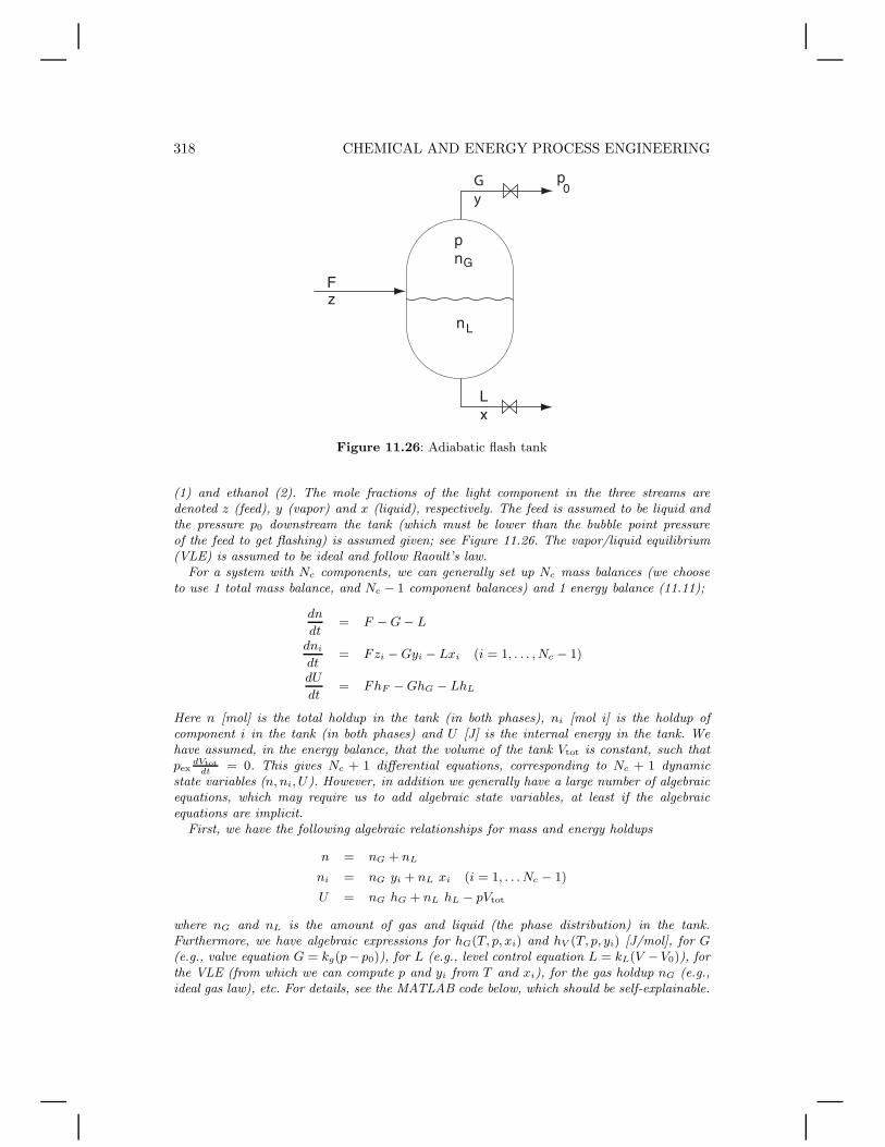
318 CHEMICAL AND ENERGY PROCESS ENGINEERING
G
y
Figure 11.26: Adiabatic flash tank
(1) and ethanol (2). The mole fractions of the light component in the three streams aredenoted z (feed), y (vapor) and x (liquid), respectively. The feed is assumed to be liquid andthe pressure p0 downstream the tank (which must be lower than the bubble point pressureof the feed to get flashing) is assumed given; see Figure 11.26. The vapor/liquid equilibrium(VLE) is assumed to be ideal and follow Raoult’s law.
For a system with Nc components, we can generally set up Nc mass balances (we chooseto use 1 total mass balance, and Nc − 1 component balances) and 1 energy balance (11.11);
dn
dt= F − G − L
dni
dt= Fzi − Gyi − Lxi (i = 1, . . . , Nc − 1)
dU
dt= FhF − GhG − LhL
Here n [mol] is the total holdup in the tank (in both phases), ni [mol i] is the holdup ofcomponent i in the tank (in both phases) and U [J] is the internal energy in the tank. Wehave assumed, in the energy balance, that the volume of the tank Vtot is constant, such thatpex
dVtotdt
= 0. This gives Nc + 1 differential equations, corresponding to Nc + 1 dynamicstate variables (n, ni, U). However, in addition we generally have a large number of algebraicequations, which may require us to add algebraic state variables, at least if the algebraicequations are implicit.
First, we have the following algebraic relationships for mass and energy holdups
n = nG + nL
ni = nG yi + nL xi (i = 1, . . . Nc − 1)
U = nG hG + nL hL − pVtot
where nG and nL is the amount of gas and liquid (the phase distribution) in the tank.Furthermore, we have algebraic expressions for hG(T, p, xi) and hV (T, p, yi) [J/mol], for G(e.g., valve equation G = kg(p− p0)), for L (e.g., level control equation L = kL(V −V0)), forthe VLE (from which we can compute p and yi from T and xi), for the gas holdup nG (e.g.,ideal gas law), etc. For details, see the MATLAB code below, which should be self-explainable.
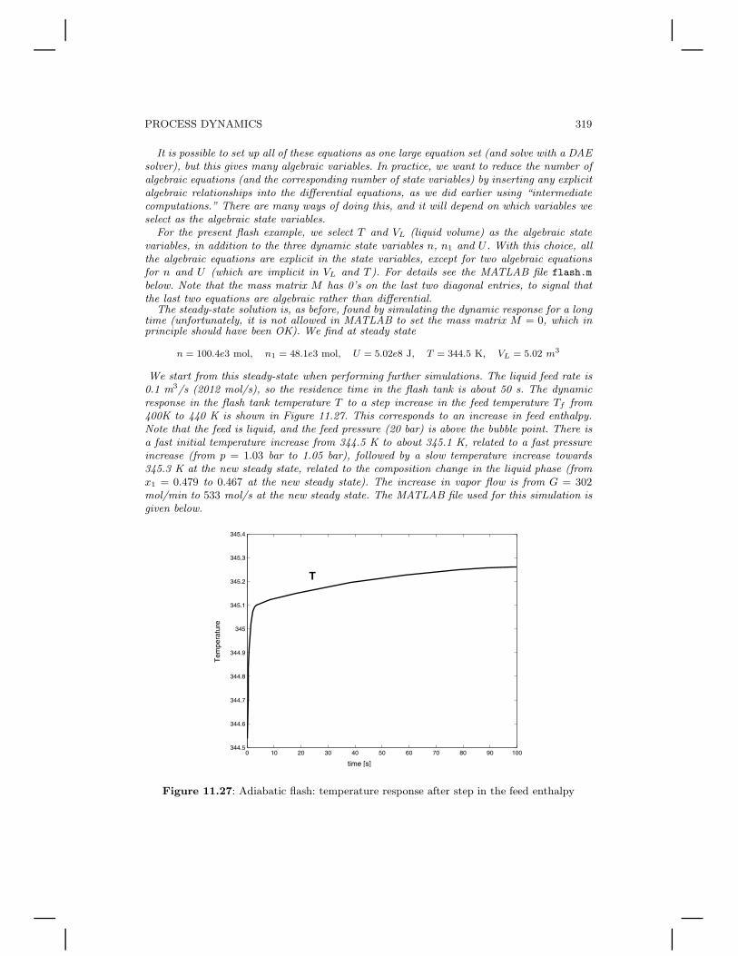
PROCESS DYNAMICS 319
It is possible to set up all of these equations as one large equation set (and solve with a DAEsolver), but this gives many algebraic variables. In practice, we want to reduce the number ofalgebraic equations (and the corresponding number of state variables) by inserting any explicitalgebraic relationships into the differential equations, as we did earlier using “intermediatecomputations.” There are many ways of doing this, and it will depend on which variables weselect as the algebraic state variables.
For the present flash example, we select T and VL (liquid volume) as the algebraic statevariables, in addition to the three dynamic state variables n, n1 and U . With this choice, allthe algebraic equations are explicit in the state variables, except for two algebraic equationsfor n and U (which are implicit in VL and T ). For details see the MATLAB file flash.m
below. Note that the mass matrix M has 0’s on the last two diagonal entries, to signal thatthe last two equations are algebraic rather than differential.
The steady-state solution is, as before, found by simulating the dynamic response for a longtime (unfortunately, it is not allowed in MATLAB to set the mass matrix M = 0, which inprinciple should have been OK). We find at steady state
n = 100.4e3 mol, n1 = 48.1e3 mol, U = 5.02e8 J, T = 344.5 K, VL = 5.02 m3
We start from this steady-state when performing further simulations. The liquid feed rate is0.1 m3/s (2012 mol/s), so the residence time in the flash tank is about 50 s. The dynamicresponse in the flash tank temperature T to a step increase in the feed temperature Tf from400K to 440 K is shown in Figure 11.27. This corresponds to an increase in feed enthalpy.Note that the feed is liquid, and the feed pressure (20 bar) is above the bubble point. There isa fast initial temperature increase from 344.5 K to about 345.1 K, related to a fast pressureincrease (from p = 1.03 bar to 1.05 bar), followed by a slow temperature increase towards345.3 K at the new steady state, related to the composition change in the liquid phase (fromx1 = 0.479 to 0.467 at the new steady state). The increase in vapor flow is from G = 302mol/min to 533 mol/s at the new steady state. The MATLAB file used for this simulation isgiven below.
0 10 20 30 40 50 60 70 80 90 100344.5
344.6
344.7
344.8
344.9
345
345.1
345.2
345.3
345.4
Tem
pera
ture
time [s]
T
Figure 11.27: Adiabatic flash: temperature response after step in the feed enthalpy
320 CHEMICAL AND ENERGY PROCESS ENGINEERING
function F=f(t,y)% This is file flash.m% INPUT: Time t and state vector y% OUTPUT: Right hand side of DAE set: M dy/dt = f(y)% States n=y(1); n1=y(2); U=y(3); T=y(4); VL=y(5);% Usage with ode15s:% options = odeset(’mass’,diag([1 1 1 0 0]));% y0 = [100.4e3 48.1e3 5.02e8 344.5 50.17]% [t,y]= ode15s(@flash,[0 100],y0,options)% Plot temperature: plot(t,y(:,4))
% All in SI units% I. Data (parameters and independent variables)% Data for: 1-methanol, 2-ethanolA1=8.08097; B1=1582.271; C1=239.726; % Antoine psat1 [mmHg] w/ T [C] (T-range: 15C - 84C)A2=8.11220; B2=1592.864; C2=226.184; % Antoine psat2 [mmHg] w/ T [C] (T-range: 20C - 93C)cpl1=80; cpl2=131; cpv1=44; cpv2=65; % heat capacity [J/K mol]T0=298.15; hvap01=38000; hvap02=43000; % heat of vap. at T0 [J/mol]Vl1= 40.7e-6; Vl2=58.7e-6; % liquid molar volumes [m3/mol]R=8.13; % J/mol K
% Feed dataq=0.1; % m3/sz1=0.5; % mol1/molTf=1.1*400; % K (increase from 400K to 440K)p0=1e5; % N/m2 (=1 bar downstream pressure)Vf = z1*Vl1 + (1-z1)*Vl2; % m3/mol (molar volume feed)F = q/Vf; % mol/s (feed rate)
% Total tank volumeVtot = 10; % m3
% Valve constant and controller gainkg=0.1; kl=100e3; % note that the P-controller gain kl is large
% II. Extract present value of statesn=y(1); % total holdup in tank (both phases) [mol]n1=y(2); % component 1 holdup in tank (both phases) [mol1]U=y(3); % total internal energy (both phases) [J]T=y(4); % temperature (same in both phases) [K]VL=y(5); % liquid volume [m3]
% IIIa. Intermediate calculations% VLEx1 = n1/n;p1s=10.^(A1-B1/(T-273.15+C1))/750e-5; % psat1 from Antoine [N/m2]p2s=10.^(A2-B2/(T-273.15+C2))/750e-5; % psat2 from Antoine [N/m2]p1 = x1*p1s; % partial pressure component 1 [N/m2]p2 = (1-x1)*p2s; % partial pressure component 2 [N/m2]p = p1+p2; % pressure = sum of partial pressures [N/m2]y1 = p1/p; % vapor fraction component 1 [mol1/mol]Vm = x1*Vl1 + (1-x1)*Vl2; % molar volume (liquid phase) [m3/mol]
% Phase distributionVG = Vtot - VL; % gas volume [m3]nL = VL / Vm; % liquid holdup [mol]nG = p*VG / (R*T); % gas holdup (ideal gas law) [mol]
% Enthalpies [J/mol] (Ref.state: pure liquid at T0)hF = [z1*cpl1 + (1-z1)*cpl2] * (Tf-T0);hL = [x1*cpl1 + (1-x1)*cpl2] * (T -T0);hG = [y1*cpv1 + (1-y1)*cpv2] * (T -T0) + y1*hvap01 + (1-y1)*hvap02;
PROCESS DYNAMICS 321
% Vapor and liquid flowG = kg*(p-p0); % simple valve equation for outflow of gas [mol/s]VLs = Vtot/2; % Setpoint level (volume): keep 50% liquid in tank [m3]L = kl*(VL-VLs); % Level controller with proportional gain kl [mol/s]
% IIIb. Evaluate right hand side of DAE-set: M dy/dt = f(y)f1 = F - G - L; % =dn/dt Dynamic: Overall mass balancef2 = F*z1 - G*y1 - L*x1; % =dn1/dt Dynamic: Component 1 mass balancef3 = F*hF - G*hG - L*hL; % =dU/dt Dynamic: Energy balancef4 = U + p*Vtot - hL*nL - hG*nG; % = 0 Algebraic: Internal energy Uf5 = n - nG - nL; % = 0 Algebraic: Total holdup nF = [f1; f2; f3; f4; f5];
Finding the steady-state. Above, the steady state was found by simulating the dynamicresponse for a long time. Alternatively, one may find the steady-state directly, for example,using the function fmincon in MATLAB:
yss = fmincon(’1’,y0,[],[],[],[],[],[],@flashss)
where the file flashss.m is identical to flash.m (above) except that the first line is changedto function [c,ceq]=f(y) and the following line is added at the end: c=[]; ceq=F;.
Remark 1 Removing or adding algebraic state variables. In the MATLAB code givenabove, we have two algebraic state variables (T and VL), but actually we can get rid of VL asa state variable if we do a little work. This follows because the holdup equations are simple,so we can combine them (including n = nG + nL which MATLAB solved using f5 in thecode above), and derive an explicit expression for VL as a function of n, p, Vtot and Vm (tryyourself, it is easy!). In the MATLAB code above, we then replace the line VG = Vtot - VLby the following two lines of “intermediate calculations”:
VG = (Vtot-n*Vm)/(1 - (p*Vm)/(R*T));VL = Vtot - VG;
We now have only 4 state variables, so we delete the algebraic equation f5 = n - nG - nL
at the end. Of course, we also need to change the mass matrix and the call to ode15s. Thefinal result is of course the same as before.
The main problem when we reduce the number of state variables is that the equations geta bit more messy and it is easy to make mistakes. For this reason, we often choose to add“unnecessary” state variables in the problem. This also makes plotting the results easier, asMATLAB stores all the state variables. For example, if we want to plot pressure, then we cansimply add a “dummy” state variable (pdummy=y(6);) together with a “dummy” algebraicequation (f6= p - pdummy;).
Remark 2 Fixing pressure and index problem. In the model of the flash tank givenin the MATLAB code above, we let the pressure vary dynamically, but from the very quickinitial rise in temperature in Figure 11.27 it follows that the pressure dynamics are veryfast. In such cases it might be tempting to say that the pressure is fixed by introducing thealgebraic equation p = p0 (f6 = p-p0;) and an additional state variable G (and omittingthe valve equation for G). This is in principle OK, but it turns out that the integrationroutine ode15s is unable to solve this – we get an error message: “This DAE appears to
be of index greater than 1.” An “index problem” is often an indication of a non-physicalassumption (in this case, it is not physically possible to keep the pressure p constant), andthe problem can often be avoided by rewriting the equations, and/or avoiding non-physicalassumptions.
322 CHEMICAL AND ENERGY PROCESS ENGINEERING
11.6 Process control
Automatic feedback control is widely used in the process industry, and theinstrumentation and control system typically represents 30% of the investments ina plant. For each process variable y that one wants to control one needs
• a measurement of the process variable (y),• an independent manipulated variable u (usually a valve) that influences y.
We use the following notation
• CV = controlled variable (y, “output”)• MV = manipulated variable (u, “input”, independent variable)• DV = disturbance variable (d, independent variable that we cannot influence)
The MV should have a “direct” and large effect on the CV (with fast dynamics anda small delay or inverse response). The idea of control is to adjust the MV (u) suchthat the CV (y) is kept close to its desired setpoint ys, in spite of disturbances d, thatis, we want a small control error,
e(t) = y(t) − ys
We use negative feedback, where the sign of the control action is opposite thesign of the process. This implies that the MV (u) is adjusted such that it counteractschanges in the CV (y). A well-known feedback controller from daily life is the on/offcontroller used in thermostats, where the heat is the MV and temperature is the CV.The on/off controller is simple, but it gives large MV changes (between max andmin), and fluctuations in the CV (temperature) are unavoidable. This is undesirable,so in the process industry one normally uses the proportional-integral-derivative (PID)controller with algorithm
u(t) = u0 − Kc
(
e(t) +1
τI
∫ t
0
e(t)dt + τDde(t)
dt
)
(11.54)
We see that the MV-change away from its nominal value (u − u0) is a weighted sumof the present value of the error e (the P-term), the integral of the error e (the I-term)and the derivative of the error e (the D-term). The PID controller has three adjustableparameters:
• Gain Kc
• Integral time τI [s]• Derivative time τD [s]
The proportional term is usually the most important, and a large value of Kc resultsin a faster initial response. The integral action causes the MV to change until theerror e(t) is zero, that is, we get no steady state off-set. A small value of the integraltime τI [s] results in the controller returning faster to steady state. For this reason,the integral time is often called the “reset time.” The derivative term can give fasterresponses for some processes, but it often gives “nervous control” with large sensitivityto measurement noise. For this reason, a PI controller (with τD = 0) is most common.

PROCESS DYNAMICS 323
There are also other variants of the PID controller, for example, the cascade form,but the differences are usually small for practical purposes. One should, however, notethat the vendors use different names and definitions for the three PID parameters.For example, some vendors use the integral gain KI = Kc/τI and the derivative gainKD = KcτD. Others use the “proportional band” 100/Kc, and “reset rate” 1/τI .
The main problem with negative feedback is that we can get instability if we over-react (if Kc is too large or τI is too small) such that we get variations that grow overtime.
On-line tuning. Finding good control parameters (“tunings”) is not as simpleas one may believe. A common (and serious) mistake is to use the wrong sign forKc, which usually causes the system to drift to an operating point with a fully openor fully closed valve. Tuning is often performed “on-line” using trial-and-error. Oneusually starts with a controller with a low gain (Kc) and with no integral action(τI = ∞). Kc is then gradually increased until either (a) the control performance todisturbances and set-point changes is acceptable, (b) the MV change is too large or(c) the system starts oscillating. If the system starts oscillating, then Kc is reducedby approximately a factor 2 or more. Next, one gradually reduces the integral time τI
until (a) the settling time (back to the set-point) is acceptable or (b) the system startsoscillating. If the system oscillates, then τI is increased by a factor of approximately 2or more compared to the value that gave oscillations. If the response is too slow thenone may try introducing derivative time τD, which can be increased until (a) the MVchanges become too nervous or (b) the system starts oscillating. If the system startsoscillating, then τD is reduced with approximately a factor 2 or more compared to thevalue that gave oscillations.
Model-based tuning for fast response. Alternatively, model-based tuning isused. The response (without control) from the MV (u) to the CV (y) is recordedand then approximated as a first-order response with a delay, that is, one obtainsthe model parameters k, τ and θ (see page 286). The following SIMC4 PI-tunings arerecommended
Kc =1
k
τ
τc + θ; τI = min{τ, 4(τc + θ)} (11.55)
Here, the “closed-loop” response time τc [s] is the only tuning parameter. A smaller τc
gives a faster response for the CV, but one may get oscillations and the MV-changesare larger. In order to avoid oscillations and have good robustness (with a good marginto instability), it is recommended to choose τc larger than the effective delay, that is,τc ≥ θ.
If the response is dominant second order, meaning that the response is wellapproximated by a second-order response with τ2 > θ, then a substantial improvementcan sometimes be obtained by adding derivative action, provided there is not too muchmeasurement noise. The response is then approximated by a second-order model withparameters k, τ, τ2 and θ. For a PID controller on cascade form, Kc and τI are then asgiven in (11.55) (but note that the parameter values will change because θ is smallerwhen we use a second-order model) and the derivative time is
τD = τ2 (11.56)
4 S. Skogestad, “Simple analytic rules for model reduction and PID controller tuning,” J. ProcessControl, Vol. 13 (2003), 291–309.
324 CHEMICAL AND ENERGY PROCESS ENGINEERING
Note that this is for a so-called cascade PID-form. To get the corresponding PID-parameters for the “ideal” PID form in (11.54), compute the factor α = 1 + τD/τI ,and multiply Kc and τI by α, and divide τD by α.
Conservative tuning for smooth response. The tuning procedure outlinedabove is often time consuming, and as a starting point the following minimum(“conservative”) gain can be used5
|Kc,min| =|u0|
|ymax|(11.57)
where |u0| is the MV change required to counteract the largest expected disturbanceand |ymax| is the largest accepted CV deviation. In industry, the variables have oftenalready been scaled such that |u0| ≈ |ymax| (for example equal to 1) and we get|Kc,min| ≈ 1. Indeed, this is a common factory setting for the gain. In addition, it iscrucial that the sign of Kc is chosen correctly – remember that the control is supposedto counteract and not intensify changes in the CV. As a conservative starting pointfor the integral time, τI = τ can be chosen, where τ is the dominant time constant forthe effect of the MV on the CV.
Example 11.19 Control of exothermic CSTR. This is a continuation of Example 11.16(page 311). We want to keep the reactor temperature y = T approximately constant atys = 444K. We assume that the reactor temperature can be measured and that we can affecty = T by changing the coolant temperature u = Tc. The objective is to design a feedbackPI-controller with y = T as the controlled variable (CV) and u = Tc as the manipulatedvariable (MV). We consider, as before, an increase in the feed rate of 20% (from 0.10 to0.12 m3/min) – this is the “disturbance” to the process. Without control, we have found thatthe reactor temperature T will eventually drop to 441.9 K, but with PI control the MV willcounteract the disturbance such that CV = T returns to its desired value (setpoint) of 444 K;see Figure 11.28.
To tune the controller, we obtained first, without control, the response from the coolingtemperature (MV, u) to the reactor temperature (CV, y). This response (not shown inFigure 11.28) can be closely approximated as a first-order response (without time delay θ)with gain k = ∆y(∞)/∆u ≈ 0.5 and time constant τ ≈ 7 min. For example, this is obtainedby simulating a small step in Tc (for example, by changing Tc from 430 to Tc=431 and settingq=0.1 in the MATLAB code on page 312), but it can also be found analytically by linearizingthe model. We chose the closed-loop response time to be τc = 3 min (a lower value gives afaster response, but with larger changes in the MV Tc). From (11.55), this gives the PI-settings
Kc =1
0.5
7
3 + 0= 4.7, τI = min{7, 12} = 7 min
.The response with control is shown in Figure 11.28. We see that the temperature y = T
returns to its setpoint Ts = 444 K after about 9 minutes (about three times τc). The simulationwas performed by adding the following lines after point II in the MATLAB code on page 312:
% PI-CONTROLLER: u = u0 - Kc*e - (Kc/taui)*eint, where deint/dt = e% Note: (1) The integrated error eint is introduced as an extra state: eint = y(4)% (2) The process ‘‘output" (CV) yreg is in this case the reactor temperature T% (3) The process ‘‘input" (MV) u is in this case the cooling temperature Tcyreg = T; yregs= 444; e=yreg-yregs; u0 = 430; eint=y(4); Kc=4.7; taui=7;u = u0 - Kc*e - (Kc/taui)*eint;Tc = u;
5 S. Skogestad, “Tuning for smooth PID control with acceptable disturbance rejection,” Ind. Eng.Chem. Res., Vol. 45, 7817-7822 (2006).
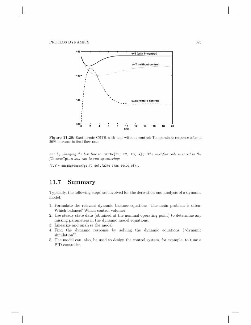
PROCESS DYNAMICS 325
0 2 4 6 8 10 12 14 16 18 20430
435
440
445
time
y=T (without control)
u=Tc (with PI-control)
y=T (with PI-control)
Figure 11.28: Exothermic CSTR with and without control: Temperature response after a20% increase in feed flow rate
and by changing the last line to: DYDT=[f1; f2; f3; e];. The modified code is saved in thefile cstrTpi.m and can be run by entering:
[T,Y]= ode15s(@cstrTpi,[0 50],[2274 7726 444.0 0]);.
11.7 Summary
Typically, the following steps are involved for the derivation and analysis of a dynamicmodel:
1. Formulate the relevant dynamic balance equations. The main problem is often:Which balance? Which control volume?
2. Use steady state data (obtained at the nominal operating point) to determine anymissing parameters in the dynamic model equations.
3. Linearize and analyze the model.4. Find the dynamic response by solving the dynamic equations (“dynamic
simulation”).5. The model can, also, be used to design the control system, for example, to tune a
PID controller.