S1

Supplementary Information

A Cu(II)-MOF Capable of Fixing CO2 From Air and Showing High Capacity H2 and CO2 Adsorption

Vivekanand Sharma,‡a Dinesh De,‡a Ranajit Saha,b Ranjita Das,b Pratim Kumar Chattaraj,*b and Parimal K. Bharadwaj*a

aDepartment of Chemistry, Indian Institute of Technology Kanpur, Kanpur 208016, India

bDepartment of Chemistry, Indian Institute of Technology Kharagpur, Kharagpur 721302, India

Electronic Supplementary Material (ESI) for ChemComm.This journal is © The Royal Society of Chemistry 2017

S2

Experimental Section

Materials. The metal salts and other reagent grade chemicals were purchased and used without

further purification from commercial suppliers (Sigma-Aldrich, Alfa Aesar, TCI, and others). All

the solvents were from S. D. Fine Chemicals, India. These solvents were purified following

standard conventional methods prior to use.

Physical Measurements

The following Spectroscopic data were collected. IR spectra (KBr disk, 400−4000 cm−1)

were recorded on a Perkin-Elmer model 1320 spectrometer. Powder X-ray diffraction (PXRD)

patterns were recorded with a Bruker D8 Advance diffractometer equipped with nickel-filtered

Cu Kα (1.5418 Å) radiation. The tube voltage and current were 40 kV and 40 mA, respectively.

Thermogravimetric analyses (TGA) (heating rate of 5 °C/min under nitrogen atmosphere) were

performed with a Mettler Toledo Star System. 1H NMR and 13C NMR spectra were recorded

either on a JEOL ECX 500 FT (500, 125 MHz respectively) or on a JEOL ECS 400 FT (400, 100

MHz respectively) instrument in CDCl3 or in DMSO-d6 with Me4Si as the internal standard. The

ESI-Mass data were obtained in a WATERS-Q-Tof Premier Mass Spectrometer. Melting points

were recorded on an electrical melting point apparatus from PERFIT India and were uncorrected.

Synthesis of the linker, H4L

Synthesis of the ligand 5′-amino-1,1′:4′,1″-terphenyl-3,3″,5,5″-tetracarboxylic acid (H4L;

Scheme S1) was achieved in several steps following literature procedure.1

S3

NH2

NO2

NH2

NO2

Br Br

NO2

Br Br

NH2

Br Br

NH2

Br Br EtO2C CO2Et

BHO OH

NH2

EtO2C

CO2Et

CO2Et

CO2Et

NH2

HO2C

CO2H

CO2H

CO2H

A B C D

D E F

H4L

Br2, CH3COOH NaNO2, H2SO4

EtOH THF, MeOHSnCl2

Pd(OAc)2

DMF, H2O, 60 oC

MeOH, KOH,H2O, 90 oC

(92%)(80%) (90%)

(86%)

(94%)

Scheme S1. Synthetic route for ligand H4L.

Synthesis of 2,6-dibromo-4-nitroaniline (B)

A solution of p-nitroaniline (5.00 g, 36.20 mmol) in glacial acetic acid (45 mL) was vigorously

stirred during the addition of bromine (4 mL, 78 mmol) in glacial acetic acid (28 mL) at 65 °C

for about 4 h. A very heavy precipitate formed after about 30% of the bromine had been added

and the precipitate was re-dissolved by the addition of hot water (8 mL), and then the remaining

bromine solution was added. After complete addition, the reaction continued for overnight. Then

S4

the mixture was poured into slurry of water and ice. The precipitate was filtered and washed

thoroughly with water and the dried in air. The reaction afforded 9.85 g (92% yield) of the title

compound as a yellow-green solid. 1H NMR (400 MHz, CDCl3): δ = 8.33 (s, 2H), 5.28 (br s, 2

H) ppm.

Synthesis of 3,5-dibromonitrobenzene (C).

To a stirred mixture of 2,6-dibromo-4-nitroaniline (5.00g, 16.90 mmol), ethanol (55 mL) and

concentrated sulfuric acid (6 mL) at 80°C, sodium nitrite (3.60 g, 52 mmol) was added in

portions as rapidly as effervescence would permit. The reaction mixture was allowed to stir at 80

°C for 40 h. Then the mixture was allowed to cool, poured into ice water and the solids were

collected by filtration and washed with water. The 3,5-dibromonitrobenzene was recrystallized

by dissolving in boiling ethanol and filtering the hot solution. On cooling, the reaction afforded

3.78 g (80% yield) with orange coloured crystals. 1H NMR (500 MHz, CDCl3): δ = 8.32 (d,

J=1.7 Hz, 2 H), 7.99 (t, J=1.7 Hz, 1 H) ppm.

Synthesis of 3,5-dibromoaniline(D).

To a solution of 3,5-dibromonitrobenzene (1.21 g, 39.87 mmol) in methanol (15 mL) and THF (5

mL) stirred under air, tin(II) chloride dihydrate (4.80 g, 21.27 mmol) was added in portions

slowly. The mixture was allowed to stir at about 60 °C temperature for 20 h. The solvent was

then evaporated in vacuo, and an aqueous solution of sodium hydroxide (4.16 gm in 50 ml water)

was added. The stirring was continued for 2 h. Finally, the reaction mixture was extracted with

chloroform in water. The combined organic layer was dried over Na2SO4, and the solvent was

removed in vacuo. The reaction afforded 0.98 g (90% yield) of the desired compound as a brown

solid. 1H NMR (400 MHz, CDCl3): δ = 7.00 (t, J=1.5 Hz, 1 H), 6.73 (d, J= 1.5 Hz, 2 H), 3.75 (br

s, 2 H) ppm.

S5

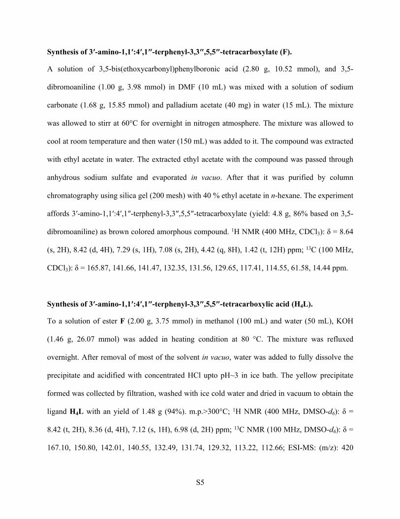
Synthesis of 3′-amino-1,1′:4′,1″-terphenyl-3,3″,5,5″-tetracarboxylate (F).

A solution of 3,5-bis(ethoxycarbonyl)phenylboronic acid (2.80 g, 10.52 mmol), and 3,5-

dibromoaniline (1.00 g, 3.98 mmol) in DMF (10 mL) was mixed with a solution of sodium

carbonate (1.68 g, 15.85 mmol) and palladium acetate (40 mg) in water (15 mL). The mixture

was allowed to stirr at 60°C for overnight in nitrogen atmosphere. The mixture was allowed to

cool at room temperature and then water (150 mL) was added to it. The compound was extracted

with ethyl acetate in water. The extracted ethyl acetate with the compound was passed through

anhydrous sodium sulfate and evaporated in vacuo. After that it was purified by column

chromatography using silica gel (200 mesh) with 40 % ethyl acetate in n-hexane. The experiment

affords 3′-amino-1,1′:4′,1″-terphenyl-3,3″,5,5″-tetracarboxylate (yield: 4.8 g, 86% based on 3,5-

dibromoaniline) as brown colored amorphous compound. 1H NMR (400 MHz, CDCl3): δ = 8.64

(s, 2H), 8.42 (d, 4H), 7.29 (s, 1H), 7.08 (s, 2H), 4.42 (q, 8H), 1.42 (t, 12H) ppm; 13C (100 MHz,

CDCl3): δ = 165.87, 141.66, 141.47, 132.35, 131.56, 129.65, 117.41, 114.55, 61.58, 14.44 ppm.

Synthesis of 3′-amino-1,1′:4′,1″-terphenyl-3,3″,5,5″-tetracarboxylic acid (H4L).

To a solution of ester F (2.00 g, 3.75 mmol) in methanol (100 mL) and water (50 mL), KOH

(1.46 g, 26.07 mmol) was added in heating condition at 80 °C. The mixture was refluxed

overnight. After removal of most of the solvent in vacuo, water was added to fully dissolve the

precipitate and acidified with concentrated HCl upto pH~3 in ice bath. The yellow precipitate

formed was collected by filtration, washed with ice cold water and dried in vacuum to obtain the

ligand H4L with an yield of 1.48 g (94%). m.p.>300°C; 1H NMR (400 MHz, DMSO-d6): δ =

8.42 (t, 2H), 8.36 (d, 4H), 7.12 (s, 1H), 6.98 (d, 2H) ppm; 13C NMR (100 MHz, DMSO-d6): δ =

167.10, 150.80, 142.01, 140.55, 132.49, 131.74, 129.32, 113.22, 112.66; ESI-MS: (m/z): 420

S6

(100%) [M-H]. Anal. calcd. for C22H15NO8: C, 62.71; H, 3.59; N, 3.32%. Found: C, 62.94; H,

3.71; N, 3.37%.

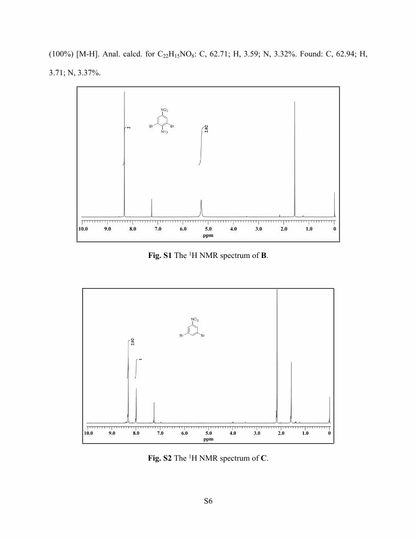
Fig. S1 The 1H NMR spectrum of B.

Fig. S2 The 1H NMR spectrum of C.

S7

Fig. S3 The 1H NMR spectrum of D.

Fig. S4 The 1H NMR spectrum of F.

S8

Fig. S5 The 13C NMR spectrum of F.

Fig. S6 The 1H NMR spectrum of H4L.

S9

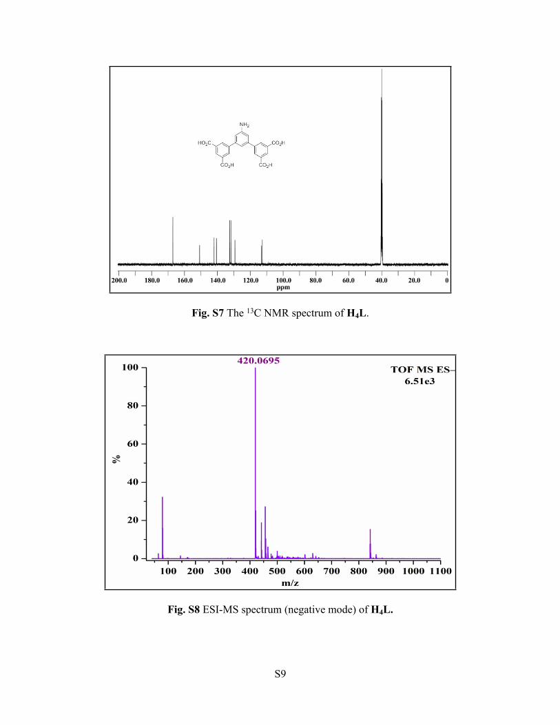
Fig. S7 The 13C NMR spectrum of H4L.

Fig. S8 ESI-MS spectrum (negative mode) of H4L.

S10

Synthesis of {[Cu6(L)3(H2O)6]∙(14DMF)(9H2O)}n (1). Cu(NO3)2·3H2O (25 mg, 0.104 mmol),

and H4L (20 mg, 0.048 mmol) were dissolved in 2mL DMF, 1 mL H2O, and one drop conc. HCl.

The mixture was placed in a Teflon-lined stainless steel autoclave and heated under autogenous

pressure to 90 °C for 3 days and then allowed to cool to room temperature. Blue colored needle

shaped crystals of 1 were collected by filtration and washed with DMF. Finally the crystal was

dried in the air. Yield ∼57%. FTIR (KBr pellets): 3422.63 cm-1 (broad), 2929.66 cm-1 (m),

1662.96 cm-1 (m), 1587.17 cm-1 (s), 1367.69 cm-1 (m), 1098.30 cm-1 (s), 776.63 cm-1 (s), 730.99

cm-1 (s). Anal. Calcd. For C108H161N17O53Cu6: C, 44.32; H, 5.54; N, 8.14%. Found: C, 44.67; H,

5.71; N, 8.21%.

General Procedure for the Coupling of Epoxides with CO2. Epoxide (20 mmol), catalyst 1′

(0.2 mol % per copper paddlewheel unit) and co-catalyst Bu4NBr (1 mmol) were taken in a

schlenk tube. The reaction mixture was then stirred at room temperature under CO2 (99.999%)

bubbling. When the reaction was completed, 5 mL CH2Cl2 was added and the mixture was

filtered to separate the catalyst. All cyclic carbonates were isolated by column chromatography

and analyzed through 1H NMR spectroscopy.

In a similar way, the conversion of atmospheric CO2 into cyclic carbonate was carried

out. Instead of using CO2 from direct source, we have purged the laboratory air as CO2 source

and the mixture was allowed to stir for 24 h.

X-Ray Structural Studies

The crystal data for 1 has been collected on a Bruker SMART CCD diffractometer (Mo

Kα radiation, λ = 0.71073 Å). The program SMART2 was used for collecting frames of data,

S11

indexing reflections, and determining lattice parameters, SAINT2 for integration of the intensity

of reflections and scaling, SADABS3 for absorption correction, and SHELXTL4 for space group

and structure determination and least-squares refinements on F2. The crystal structure were

solved and refined by full-matrix least-squares methods against F2 by using the program

SHELXL-20145 using Olex-2 software.6 All the non-hydrogen atoms were refined with

anisotropic displacement parameters. Hydrogen positions were fixed at calculated positions and

refined isotropically. The lattice solvent molecules of 1 could not be modeled satisfactorily due

to the presence of severe disorder. Therefore, PLATON/SQUEEZE7 program has been

performed to discard those disordered solvents molecules. Crystallographic data has been

deposited at the Cambridge Crystallographic Data Center and CCDC number: 1555358. Lattice

parameters of the compound, data collection and refinement parameters are summarized in Table

S1 and selected bond distances and bond angles are given in Table S2.

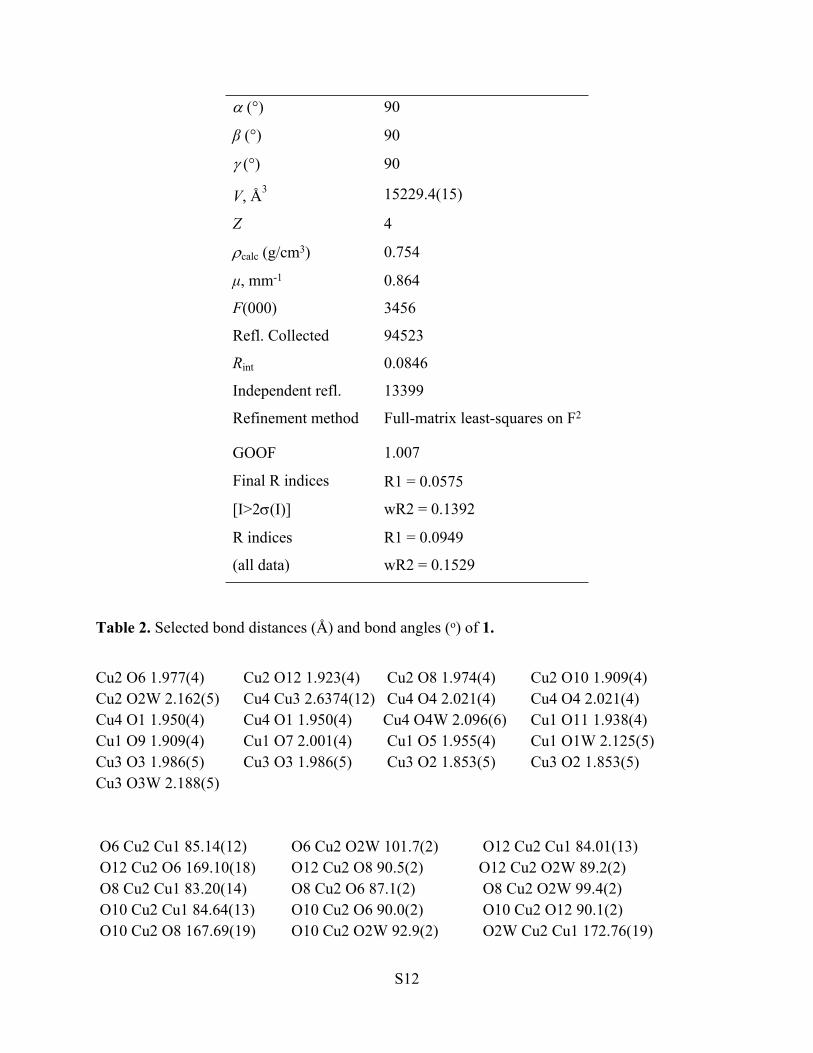
Table S1. Crystal and structure refinement data.

Parameters 1

Empirical formula C108H161N17O53Cu6

Formula wt. 2926.786

Temperature (K) 100(2)

Radiation Source Mo Kα

Wavelength (Å) 0.71073

Crystal system Orthorhombic

Space group Cmc21

a, Å 24.8326(16)

b, Å 33.3574(16)

c, Å 18.3852(10)

S12

(°) 90

β (°) 90

(°) 90

V, Å3 15229.4(15)

Z 4

calc (g/cm3) 0.754

μ, mm-1 0.864

F(000) 3456

Refl. Collected 94523

Rint 0.0846

Independent refl. 13399

Refinement method Full-matrix least-squares on F2

GOOF 1.007

Final R indices

[I>2(I)]

R1 = 0.0575

wR2 = 0.1392

R indices

(all data)

R1 = 0.0949

wR2 = 0.1529

Table 2. Selected bond distances (Å) and bond angles (o) of 1.

Cu2 O6 1.977(4) Cu2 O12 1.923(4) Cu2 O8 1.974(4) Cu2 O10 1.909(4)Cu2 O2W 2.162(5) Cu4 Cu3 2.6374(12) Cu4 O4 2.021(4) Cu4 O4 2.021(4)Cu4 O1 1.950(4) Cu4 O1 1.950(4) Cu4 O4W 2.096(6) Cu1 O11 1.938(4)Cu1 O9 1.909(4) Cu1 O7 2.001(4) Cu1 O5 1.955(4) Cu1 O1W 2.125(5)Cu3 O3 1.986(5) Cu3 O3 1.986(5) Cu3 O2 1.853(5) Cu3 O2 1.853(5)Cu3 O3W 2.188(5)

O6 Cu2 Cu1 85.14(12) O6 Cu2 O2W 101.7(2) O12 Cu2 Cu1 84.01(13) O12 Cu2 O6 169.10(18) O12 Cu2 O8 90.5(2) O12 Cu2 O2W 89.2(2) O8 Cu2 Cu1 83.20(14) O8 Cu2 O6 87.1(2) O8 Cu2 O2W 99.4(2) O10 Cu2 Cu1 84.64(13) O10 Cu2 O6 90.0(2) O10 Cu2 O12 90.1(2) O10 Cu2 O8 167.69(19) O10 Cu2 O2W 92.9(2) O2W Cu2 Cu1 172.76(19)

S13

O4 Cu4 Cu3 84.11(11) O4 Cu4 Cu3 84.11(11) O4 Cu4 O4 87.6(3) O4 Cu4 O4W 96.4(2) O4 Cu4 O4W 96.4(2) O1 Cu4 Cu3 82.49(12) O1 Cu4 Cu3 82.50(12) O1 Cu4 O4 166.17(17) O1 Cu4 O4 166.18(17) O1 Cu4 O4 87.67(18) O1 Cu4 O4 87.67(18) O1 Cu4 O1 94.0(3) O1 Cu4 O4W 97.1(2) O1 Cu4 O4W 97.1(2) O4W Cu4 Cu3 179.3(3) O11 Cu1 Cu2 84.23(12) O11 Cu1 O7 90.86(19) O11 Cu1 O5 167.23(18) O11 Cu1 O1W 101.6(2) O9 Cu1 Cu2 82.40(13) O9 Cu1 O11 89.74(19) O9 Cu1 O7 165.80(19) O9 Cu1 O5 90.3(2) O9 Cu1 O1W 99.5(2) O7 Cu1 Cu2 83.55(13) O7 Cu1 O1W 94.3(2) O5 Cu1 Cu2 83.12(13) O5 Cu1 O7 86.0(2) O5 Cu1 O1W 91.0(2) O1W Cu1 Cu2 173.9(2) O3 Cu3 Cu4 82.50(14) O3 Cu3 Cu4 82.50(14) O3 Cu3 O3 83.9(4) O3 Cu3 O3W 94.25(18) O3 Cu3 O3W 94.25(18) O2 Cu3 Cu4 85.92(13) O2 Cu3 Cu4 85.91(13) O2 Cu3 O3 167.9(2) O2 Cu3 O3 91.2(2) O2 Cu3 O3 91.2(2) O2 Cu3 O3 167.9(2) O2 Cu3 O2 91.4(4) O2 Cu3 O3W 97.13(17) O2 Cu3 O3W 97.13(17) O3W Cu3 Cu4 175.62(16) C9 O4 Cu4 121.5(4) C23 O11 Cu1 122.5(4) C1 O6 Cu2 120.2(4) C8 O1 Cu4 126.0(4) C11 O9 Cu1 125.2(4) C22 O7 Cu1 124.4(4) C9 O3 Cu3 124.2(4) C23 O12 Cu2 123.3(4) C8 O2 Cu3 123.5(4) C22 O8 Cu2 125.8(4) C11 O10 Cu2 120.8(4) C1 O5 Cu1 123.5(4)______________________________________________________________________

S14

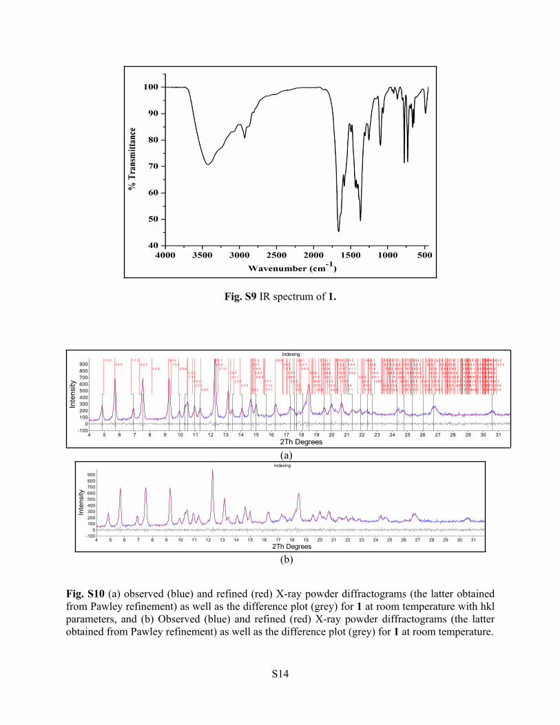
Fig. S9 IR spectrum of 1.

Indexing

2Th Degrees3231302928272625242322212019181716151413121110987654

Inte

nsity

900800700600500400300200100

0-100

1 1 00 2 0

1 1 10 2 1

2 0 0

0 0 21 3 0

2 2 01 1 21 3 1

0 2 22 2 1

0 4 0

0 4 12 0 2

3 1 01 3 2

3 1 12 2 2

2 4 00 4 2

1 1 32 4 11 5 03 3 00 2 3

1 5 13 1 23 3 1

4 0 02 4 21 3 3

2 2 30 6 0

4 2 01 5 23 3 2

0 6 14 2 10 4 3

0 0 43 1 34 0 23 5 0

2 6 0

1 1 43 5 10 2 40 6 22 6 14 2 2

2 4 34 4 0

2 0 41 5 31 7 03 3 34 4 1

5 1 01 3 41 7 1

3 5 22 2 45 1 12 6 2

0 4 44 4 20 6 35 3 0

4 2 33 1 41 7 2

5 1 25 3 1

0 8 02 4 40 8 1

3 5 33 7 02 6 3

4 6 01 1 51 5 43 3 40 2 5

3 7 15 3 2

4 6 12 8 04 4 3

6 0 00 8 22 8 1

1 7 34 0 4

5 1 35 5 0

1 3 56 2 03 7 22 2 5

0 6 45 5 14 2 44 6 2

6 2 10 4 5

2 8 21 9 0

5 3 36 0 2

3 1 53 5 41 9 12 6 45 5 2

0 8 3

6 2 26 4 02 4 5

4 4 43 7 3

6 4 14 6 31 5 5

1 7 43 3 51 9 25 1 40 0 6

2 8 34 8 0

1 1 6

0 2 64 8 13 9 05 5 30 10 06 4 25 7 0

7 1 0

6 2 30 6 53 9 15 3 40 10 14 2 55 7 12 0 6

7 1 11 3 60 8 41 9 32 2 64 8 2

2 10 07 3 0

3 5 53 7 46 6 03 9 22 6 50 10 25 7 22 10 1

0 4 64 6 47 1 27 3 16 6 1

6 4 32 8 43 1 6

4 4 56 0 4

(a) Indexing

2Th Degrees3231302928272625242322212019181716151413121110987654

Inte

nsity

900800700600500400300200100

0-100

(b)

Fig. S10 (a) observed (blue) and refined (red) X-ray powder diffractograms (the latter obtained from Pawley refinement) as well as the difference plot (grey) for 1 at room temperature with hkl parameters, and (b) Observed (blue) and refined (red) X-ray powder diffractograms (the latter obtained from Pawley refinement) as well as the difference plot (grey) for 1 at room temperature.

S15

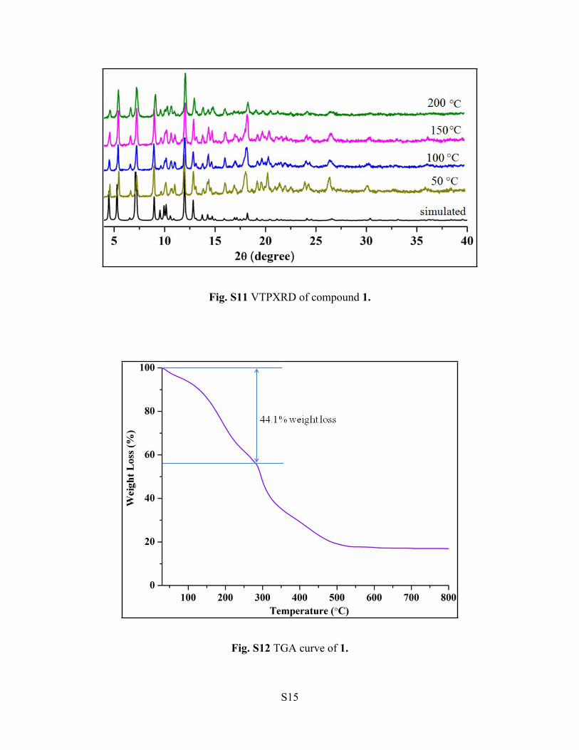
Fig. S11 VTPXRD of compound 1.

Fig. S12 TGA curve of 1.

S16

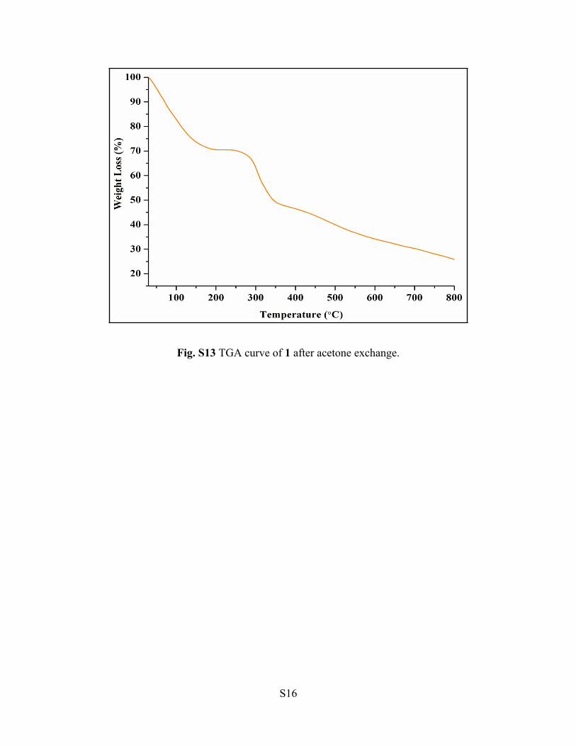
Fig. S13 TGA curve of 1 after acetone exchange.

S17

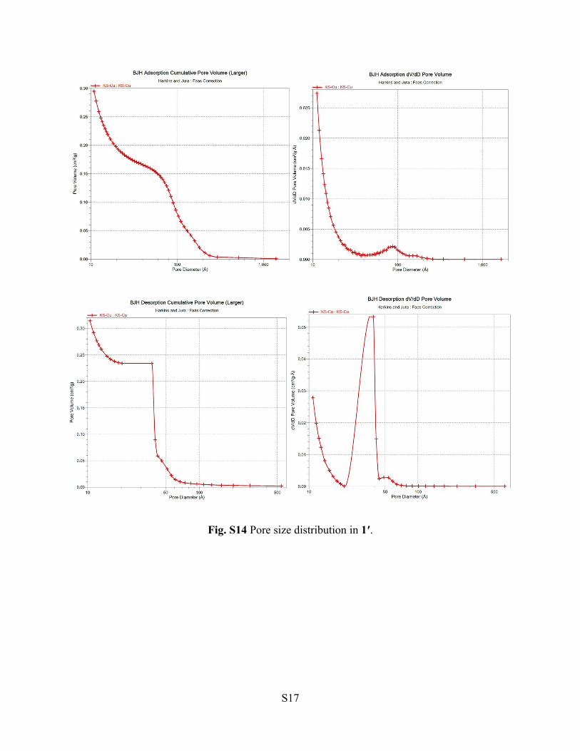
Fig. S14 Pore size distribution in 1′.

S18

Fig. S15 CH4 physisorption isotherm for 1′ at 298 K.

Calculation of Isosteric Heat of CO2 Adsorption (qst)

The process to calculate heat of CO2 adsorption from Clausius-Clapeyron equation is as

follows. Two different adsorption isotherms that were measured at different temperatures T1

(273K) and T2 (298K) are needed for the analysis. qst at an adsorption amount can be calculated

from the equation below with the difference between the two different pressures (p1 and p2) at

the same adsorption amount.

Where R is the universal gas constant.

S19

Table S3. Summary of hydrogen uptake of some selected MOFs.

Material H2 uptake at 77K and high pressure (wt %)

Volumetric H2 uptake at 77 K

(g L−1)

Reference

[Cu6(L)3(H2O)6]∙(14DMF)(9H2O) 6.6, 62 bar 49, 62 bar This Work

UMCM-150, Cu3(bhtc)2 5.7, 45 bar 36, 45 bar 8

Be12(OH)12(BTB)4 6, 20 bar 44, 100 bar 9

Cu2(abtc) 5.22, 50 bar 40.1, 50 bar 10

DUT-6, Zn4O(2,6-ndc)(btb)4/3 5.64, 50 bar 23.1, 50 bar 11

DUT-9, Ni5O2(btb)2 5.85, 40 bar 29.0, 40 bar 12

FJI-1, Zn6(BTB)4(4,4'-bipy)3 6.52, 37 bar 13

IRMOF-20, Zn4O(ttdc)2 6.7, 80 bar 34, 80 bar 14

MIL-101, Cr3OF(BDC)3 6.1, 80 bar 15

Mn-BTT, Mn3[(Mn4Cl)3(BTT)8]2 5.1, 90 bar 43, 90 bar 16

MOF-5, IRMOF-1, Zn4O(BDC)3 5.75, 35 bar

7.1, 40 bar

10, 100 bar

42.1, 40 bar

66, 100 bar

17

18

18

MOF-177, Zn4O(BTB)2 7.5, 70 bar 32, 70 bar 19

MOF-200,

Zn4O(BBC)2(H2O)3·H2O

6.9, 80 bar 36, 80 bar 20

MOF-205, Zn4O(BTB)4/3(NDC) 6.5, 80 bar 46, 80 bar 20

MOF-210, Zn4O(BTE)4/3(BPDC) 7.9, 80 bar 44, 80 bar 20

NOTT-101, Cu2(tptc) (5.71, 20 bar); (6.19, 60 bar) 43.1, 60 bar 21

NOTT-102, Cu2(qptc) (5.72, 20 bar); (6.72, 60 bar) 42.3, 60 bar 21

NOTT-103, Cu2(ndip) (6.11, 20 bar); (7.72, 60 bar) 50, 60 bar 21

NOTT-105, Cu2(ftptc) 5.12, 20 bar 21

NOTT-110, Cu2(phdip) 5.43, 55 bar 46.8, 55 bar 22

NU-100, Cu3(ttei) 9.05, 56 bar 23

PCN-10, Cu2(aobtc) 5.23, 45 bar 39.2, 45 bar 24

PCN-11, Cu2(sbtc) 5.04, 45 bar 37.8, 45 bar 24

SNU-5, Cu2(abtc) 5.22, 50 bar 45.8, 50 bar* 10

S20

Table S4. Summary of CO2 uptake of some selected MOFs.

CapacityChemical Formula Common Name

Framework

Density (g/cm3)

P (bar) T (K)

cm3/g cm3/cm3 wt %

Reference

[Cu6(L)3(H2O)6]∙(14DMF)

(9H2O)

1 0.754 32 298 289.96 218.63 60 This work

Cr3O(H2O)2F(NTC)1.5 MIL-102 1.96 30 304 66.18 129.71 13.0 25

Zn6O4(OH)4(BDC)6 UiO-66 1.238 18 303 123.71 153.15 24.3 26

Cr3O(H2O)2F(BDC)3 MIL-101(Cr) 0.62 5.3 283 132.36 82.06 26.0 27

Al(OH)(ndc) DUT-4 0.773 10 303 134.40 103.89 26.4 28

Zn2(BPnDC)2(bpy) SNU-9 1.124 30 298 152.22 171.09 29.9 29

Cu3(BTC)2 HKUST-1 0.96 300 313 217.89 209.18 42.8 30

Cr3O(H2O)3F(BTC)2 MIL-100(Cr) 0.70 50 304 225.02 157.51 44.2 31

Cu4(TDCPTM) NOTT-140 0.677 20 293 235.20 159.23 46.2 32

[Cu(H2O)]3(btei) PCN-61 0.56 35 298 258.62 144.83 50.8 33

[Cu(H2O)]3(ntei) PCN-66 0.45 35 298 272.87 122.79 53.6 33

Ni2(dobdc) Ni-MOF-74 1.206 22 278 275.93 332.77 54.2 34

[Cu3(H2O)]3(ptei) PCN-68 0.38 35 298 291.20 110.66 57.2 33

Zn4O(BTB)2 MOF-177 1.01 50 298 309.53 312.62 60.8 20

Ni5O2(BTB)2 DUT-9 0.467 47 298 316.14 147.64 62.1 12

Zn4O(BTB)4/3(NDC) MOF-205 0.38 50 298 318.69 121.10 62.6 20

Zn4O(BDC)3 MOF-5,

IRMOF-1

0.605 10 273 295.27 178.64 58.0 35

Mg2(dobdc) Mg-MOF-74 0.909 36 278 350.76 318.84 68.9 34

Cu3(TCEPEB) NU-100 0.273 40 298 355.34 97.01 69.8 36

Zn4O(BBC)2(H2O)3 MOF-200 0.22 50 298 376.22 82.77 73.9 20

Zn4O(BTE)4/3(BPDC) MOF-210 0.25 50 298 377.75 94.44 74.2 20

S21

Computational Details

We have extracted and simplified the metal organic framework (MOF) structure for the

computational study, from the associated experimental crystallographic data of the synthesized

MOF. This model for the MOF is necessary in order to reduce the computational cost keeping all

relevant interactions intact. We have studied the adsorption of H2 and CO2 gas molecules at

different positions of the model complex. All of the structures are optimized using density

functional theory (DFT) based B97x-D37 functional in conjunction with TZVP basis set. The

frequency calculations are performed at B97x-D/TZVP level of theory taking the optimized

structures. All real frequency values ensure that the optimized structures are at the minima on

their respective potential energy surfaces.

Initially two gas molecules (H2 / CO2) were chosen to check the strength and the nature

of the interaction with the host. Later on ten more gas molecules were taken to understand

whether the interaction energy gets changed drastically and / or the change in the nature of

interaction, if any. As our modeled MOF structure has two different types of gas adsorption sites,

one is at the vicinity of the Cu-center and another is near the benzene ring, it is expected that the

adsorbed gas molecules will interact in two different ways and will exhibit two different types of

interaction energies and other related properties (as vindicated by NBO and AIM analyses). First

we optimized and characterized the 2Gas@MOF structures. We computed the interaction energy

(∆Eint) in between the 2 gas molecules and the MOF and the total interaction energy is

decomposed into different energy contributions (∆Epauli, ∆Eel, ∆Eorb, ∆Edisp). The result shows

that the ∆Eint is mainly governed by the electrostatic interaction energy (∆Eel). Next we checked

the adsorption of 12 gas molecules by MOF (5 benzene rings interact with 10 gas molecules and

remaining 2 gas molecules are attached to two different Cu-centers). The 12Gas@MOF

S22

structures were optimized. The calculation of the ∆Eint and its decomposition into different

energy terms clearly indicate that the adsorption of the gas molecules to the Cu-centers is mainly

governed by ∆Eel whereas the gas molecules at the vicinity of the benzene rings are bound with

dispersion forces (∆Edisp). Thus the calculations with 2Gas@MOF as well as 12Gas@MOF

provide meaningful insights into the overall adsorption process vis-à-vis the nature of interaction

therein.

For the 12CO2@MOF system a couple of imaginary frequencies are obtained but they

can be neglected because of their very small values. The charge (q) on each atomic centre is

obtained by natural population analysis (NPA)38 and the bond order between two atoms is

obtained from the Wiberg bond index (WBI)39 calculations using the natural bond orbital (NBO)

scheme.40 All these computations are done by using a fine grid, with 75 radial shells per atom,

and 302 angular points per shell using the Gaussian 09 suite of program package.41

The energy decomposition analysis (EDA)42 is performed at rev-PBE-D3/TZ2P//B97x-

D/TZVP level of theory using ADF 2013.01 program.43,44 The EDA decomposes the interaction

energy (∆Eint) into four energy terms, viz., the Pauli repulsion (∆Epauli), the electrostatic

interaction energy (∆Eel), the orbital interaction energy (∆Eorb), and the dispersion interaction

energy (∆Edisp) as,

∆Eint = ∆Epauli + ∆Eel + ∆Eorb + ∆Edisp (1)

The ∆Epauli represents the repulsion between the electrons in the occupied orbitals of the

interacting fragments. The ΔEel term presents the quasi-classical electrostatic interaction energy

between the fragments under consideration. In general the ΔEel term is attractive in nature. The

next attractive contribution in energy comes from the orbital interaction energy, ΔEorb, which

arises due to the charge transfer and mixing of the occupied and unoccupied orbitals between the

S23

fragments and polarization effect. The ΔEdisp represents the dispersion energy correction towards

the total attraction energy.

The topological analysis of the electron density45 is carried out at the B97x-D/TZVP

level of theory. Several density based parameters are computed to find out the nature of the

interactions. These calculations are performed using Multiwfn software package.46

Identification of the non-covalent interaction between the guest gas molecules and host

MOF is carried out using the NCIPLOT software.47,48 The NCI analysis is based on the electron

density () and its reduced density gradient (s), as,

(2)s( )

1 42 3 3

1

2 3

where, is the gradient of .

The low and low s values signify a weak, non-covalent interaction in between the molecular

pairs. The Laplacian of electron density (2) is a parameter for describing the nature of the

interaction in between the molecular pairs. But, different types of non-covalent interactions

(steric interactions, hydrogen bonds, van der Waals’ (vdW) interactions) cannot be distinguished

by 2 index itself. The eigenvalues i of electron density Hessian (second derivative) matrix

such that 2 = 1 + 2 + 3 (1 < 2 < 3), is useful in the identification of the non-covalent

interactions. The sign of the 2 varies with the nature of the interaction. As for H-bonds, 2< 0,

for steric interactions, 2> 0 and for vdW type of interaction 2≲ 0. Thus, s is plotted against

sign(2) (product of sign(2) and ). The positions of the troughs associated with the s()

S24

appearing in the 2D plot give an idea about the type of the non-covalent interaction. The real

space intermolecular interaction iso-surface is generated using VMD visualization package.49

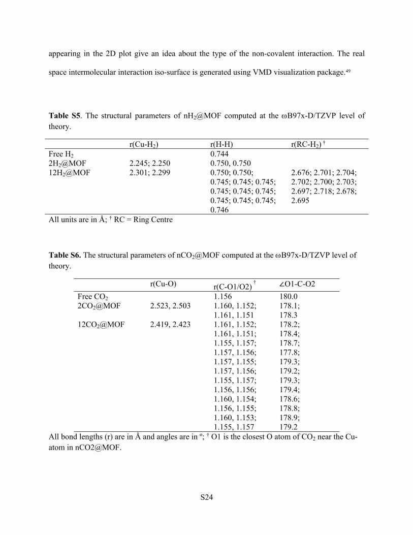
Table S5. The structural parameters of nH2@MOF computed at the B97x-D/TZVP level of theory.

r(Cu-H2) r(H-H) r(RC-H2) †

Free H2 0.7442H2@MOF 2.245; 2.250 0.750, 0.750 12H2@MOF 2.301; 2.299 0.750; 0.750;

0.745; 0.745; 0.745; 0.745; 0.745; 0.745; 0.745; 0.745; 0.745; 0.746

2.676; 2.701; 2.704; 2.702; 2.700; 2.703; 2.697; 2.718; 2.678; 2.695

All units are in Å; † RC = Ring Centre

Table S6. The structural parameters of nCO2@MOF computed at the B97x-D/TZVP level of theory.

r(Cu-O) r(C-O1/O2)

† ∠O1-C-O2Free CO2 1.156 180.02CO2@MOF 2.523, 2.503 1.160, 1.152;

1.161, 1.151178.1;178.3

12CO2@MOF 2.419, 2.423 1.161, 1.152;1.161, 1.151;1.155, 1.157;1.157, 1.156;1.157, 1.155;1.157, 1.156;1.155, 1.157;1.156, 1.156;1.160, 1.154;1.156, 1.155;1.160, 1.153;1.155, 1.157

178.2;178.4;178.7;177.8;179.3;179.2;179.3;179.4;178.6;178.8;178.9;179.2

All bond lengths (r) are in Å and angles are in º; † O1 is the closest O atom of CO2 near the Cu-atom in nCO2@MOF.

S25

Table S7. The energy decomposition analysis (EDA) results at the rev-PBE-D3/TZ2P//wB97x-D/TZVP level.

nGas@MOF Fragments ∆Epauli ∆Eel ∆Eorb ∆Edisp ∆Eint ∆Eint/Gas2H2@MOF 2H2 + MOF 21.5 -13.3 (47.5) -9.3 (33.2) -5.4 (19.3) -6.4 -3.212H2@MOF 12H2 + MOF 41.8 -19.7 (31.5) -16.2 (25.9) -26.6 (42.6) -20.7 -1.7

10H2+2H2@MOF 20.6 -6.6 (17.6) -9.8 (25.9) -21.3 (56.4) -17.1 -1.72CO2@MOF 2CO2 + MOF 32.7 -22.5 (50.5) -11.2 (25.2) -10.8 (24.2) -11.9 -6.012CO2@MOF 12CO2 + MOF 82.1 -45.9 (35.7) -23.6 (18.3) -59.3 (46.0) -46.8 -3.9

10CO2+2CO2@MOF 44.0 -20.4 (23.9) -14.0 (16.4) -50.9 (59.7) -41.3 -4.1

Table S8. Different electron density descriptors computed at B97x-D/TZVP level.

BCP points Type ρ(rc) 2ρ(rc) G(rc) K(rc) V(rc) H(rc) ELF2H2@MOFH-H (3,-1) 0.25949 -0.26505 -1.05864 0.00038 0.26505 -0.26543 1.00000Cu-H (3,-1) 0.02197 0.00070 0.07469 0.01797 -0.00070 -0.01727 0.0703912H2@MOFH-H(@Cu (3,-1) 0.25946 -0.26500 -1.05849 0.00037 0.26500 -0.26537 1.00000Cu-H (3,-1) 0.02172 0.00070 0.07352 0.01768 -0.00070 -0.01699 0.06999C-H (3,-1) 0.00438 0.00075 0.01511 0.00303 -0.00075 -0.00228 0.01212H-H(@Ar (3,-1) 0.26160 -0.26812 -1.07187 0.00015 0.26812 -0.26826 1.00000H2-H2 (3,-1) 0.00197 0.00045 0.00688 0.00127 -0.00045 -0.00082 0.00479

2CO2@MOFCu-O (3,-1) 0.02221 0.10275 0.02403 -0.00165 -0.02238 0.00165 0.04205O(in CO2)-H(aromatic ring) (3,-1) 0.00328 0.01318 0.00246 -0.00083 -0.00162 0.00083 0.00705O-C (of CO2) (3,-1) 0.46778 0.37420 0.93778 0.84423 -1.78201 -0.84423 0.42688

12CO2@MOF Cu-O (3,-1) 0.02619 0.12765 0.03043 -0.00148 -0.02895 0.00148 0.04533O(in CO2)-H(aromatic ring) (3,-1) 0.00588 0.02305 0.00449 -0.00128 -0.00321 0.00128 0.01475C(in CO2)-C(aromatic ring) (3,-1) 0.00526 0.01823 0.00364 -0.00092 -0.00271 0.00092 0.01550O(in CO2)-C(aromatic ring)

(3,-1)0.00089 0.00337 0.00058 -0.00026 -0.00032 0.00026 0.00157

O-O (of two different CO2)

(3,-1)0.00500 0.02318 0.00425 -0.00155 -0.00270 0.00155 0.00964

O-C (of two different CO2) (3,-1) 0.00534 0.02477 0.00474 -0.00145 -0.00329 0.00145 0.00961O-C (of same CO2) (3,-1) 0.45792 0.23905 0.88054 0.82077 -1.70131 -0.82077 0.44039

S26

Table S9. The NBO analysis of nH2@MOF at wB97x-D/TZVP level.

qH2 (qH,qH) q(Cu) WBI(H-H) WBI(Cu-H)Free H2 0.000 (0.000, 0.000) 1.0000

2H2@MOF 0.043 (0.021, 0.022);0.045 (0.020,0.025)

1.037;1.036

0.9522;0.9517

(0.0450, 0.0454);(0.0448,0.0446)

12H2@MOF 0.057 (0.028, 0.029);0.057 (0.025, 0.032);

-0.006 (0.012, -0.018);-0.004 (0.014, -0.018);-0.005 (0.013, -0.018);-0.006 (0.011, -0.017);-0.005 (0.012, -0.017);-0.006 (0.012, -0.018);-0.002 (0.015, -0.017);-0.001 (0.012, -0.013);-0.004 (0.009, -0.013);-0.002 (0.007, -0.009);

0.425;0.426

0.9524;0.9521;0.9983;0.9982;0.9982;0.9982;0.9982;0.9982;0.9980;0.9979;0.9980;0.9976

(0.0448, 0.0447);(0.0447,0.0445)

Table S10. The NBO analysis of nCO2@MOF at wB97x-D/TZVP level.

qCO2 (qO1, qC, qO2) q(Cu) WBI(C-O1), WBI(C-O2) WBI(Cu-O1)Free CO2 0.000 (-0.483, 0.967, -0.483) 1.9108,1.91112CO2@MOF 0.035 (-0.509, 1.018, -0.474)

0.036 (-0.514, 1.013, -0.463)1.0621.059

1.8488, 1.9358;1.8387, 1.9490

0.06230.0658

12CO2@MOF 0.044 (-0.508, 1.019, -0.467)0.045 (-0.509, 1.021, -0.467)-0.001 (-0.498, 0.984, -0.487)-0.001 (-0. 498, 0.984, -0.487)-0.001 (-0. 498, 0.985, -0.488)0.000 (-0. 489, 1.003, -0.514) 0.001 (-0.474, 0.990, -0. 515)0.001 (-0.496, 0.994, -0.497) 0.000 (-0.500, 0.988, -0.488)-0.001 (-0.477, 0.990, -0. 514)0.001 (-0.502, 0.991, -0.488)-0.001 (-0.501, 0.987, -0.487)

1.0601.062

1.8373, 1.9443;1.8381, 1.9445;1.8985, 1.9117;1.8973, 1.9117;1.8987, 1.9112;1.8832, 1.9130;1.8951, 1.9123;1.8945, 1.9109;1.8793, 1.9256;1.8778, 1.9285;1.9022, 1.9015;1.8946, 1.9121

0.08210.0827

S27

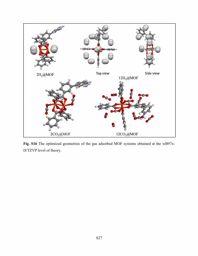
Fig. S16 The optimized geometries of the gas adsorbed MOF systems obtained at the wB97x-

D/TZVP level of theory.

S28

Fig. S17 Different critical points of the gas adsorbed MOF systems obtained at the B97x-D/TZVP level of theory.

S29

Fig. S18 (a) NCI isosurface plot of 12H2@MOF. The isosurface is generated for s = 0.5 a.u., (b) The plot of reduced gradient versus sign(λ2)ρ of the 12H2@MOF system, (c) zoomed view of the plot of reduced gradient versus sign(λ2)ρ of the 12H2@MOF system.

S30

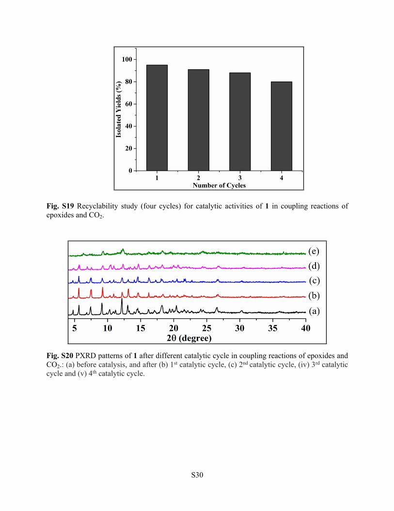
Fig. S19 Recyclability study (four cycles) for catalytic activities of 1 in coupling reactions of epoxides and CO2.

Fig. S20 PXRD patterns of 1 after different catalytic cycle in coupling reactions of epoxides and CO2.: (a) before catalysis, and after (b) 1st catalytic cycle, (c) 2nd catalytic cycle, (iv) 3rd catalytic cycle and (v) 4th catalytic cycle.

S31

NMR of Catalysis Experiments

Coupling Reactions of Epoxides and CO2

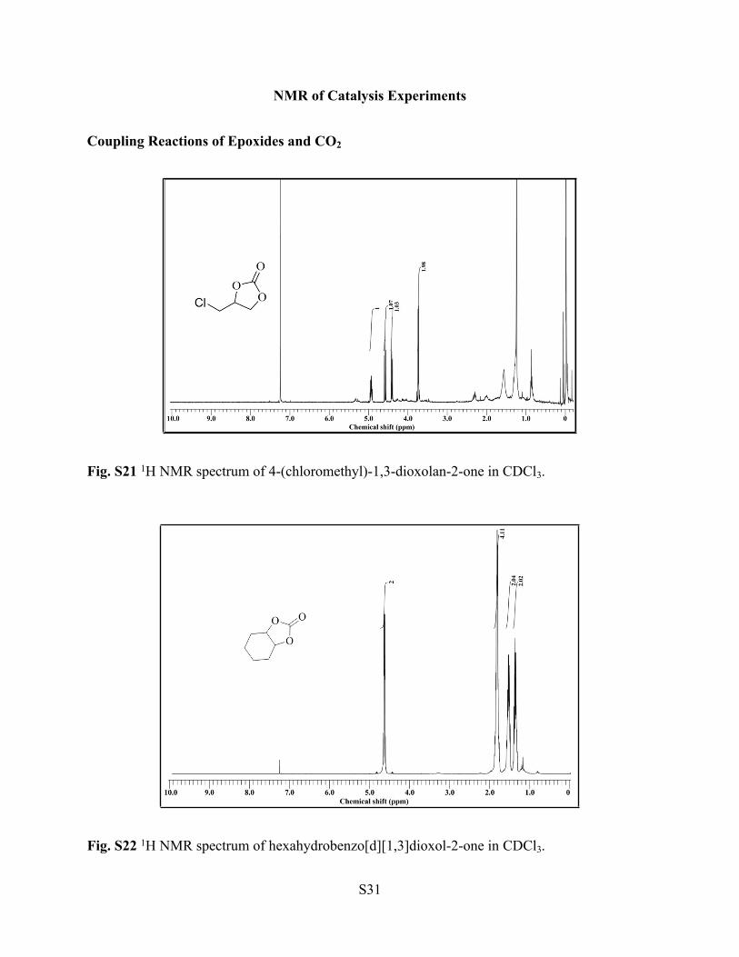
Fig. S21 1H NMR spectrum of 4-(chloromethyl)-1,3-dioxolan-2-one in CDCl3.

Fig. S22 1H NMR spectrum of hexahydrobenzo[d][1,3]dioxol-2-one in CDCl3.

S32

Fig. S23 1H NMR spectrum of 4-phenyl-1,3-dioxolan-2-one in CDCl3.

Fig. S24 1H NMR spectrum of 4-(phenoxymethyl)-1,3-dioxolan-2-one in CDCl3.

S33

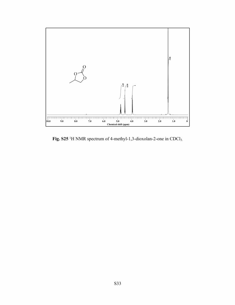
Fig. S25 1H NMR spectrum of 4-methyl-1,3-dioxolan-2-one in CDCl3.

S34

O

R

OO

O

R

O

O

OR

OR

Br

O

R

R'4NBr

R'4N

OR

Br

C OOC OO

R'4N

O

R

R' 4NBr

Scheme S2. Proposed mechanism for the 1′ catalyzed carbon dioxide fixation into epoxide in the presence of TBAB.

REFERENCES

1 (a) D. De, T. K. Pal, S. Neogi, S. Senthilkumar, D. Das, S. S. Gupta and P. K. Bharadwaj, Chem. Eur. J., 2016, 22, 3387–3396; (b) S. H. Chanteau and J. M. Tour,. J. Org. Chem., 2003, 68, 8750–8766.

2 SMART & SAINT Software Reference manuals, Version 6.45; Bruker Analytical X-ray

S35

Systems, Inc.: Madison, WI, 2003.

3 G. M. Sheldrick, SADABS, a software for empirical absorption correction, Ver. 2.05; University of Göttingen: Göttingen, Germany, 2002.

4 (a) SHELXTL Reference Manual, Ver. 6.1; Bruker Analytical X-ray Systems, Inc.: Madison, WI, 2000; (b) G. M. Sheldrick, SHELXTL, Ver. 6.12; Bruker AXS Inc.: WI. Madison, 2001.

5 G. M. Sheldrick, Acta Crystallogr. Sect. A: Fundam. Crystallogr., 2008, 64, 112–122.

6 O. V. Dolomanov, L. J. Bourhis, R. J. Gildea, J. A. K. Howard and H. Puschmann, J. Appl. Crystallogr., 2009, 42, 339–341.

7 A. L. Spek, J. Appl. Cryst., 2003, 36, 7–13.

8 A. G. Wong-Foy, O. Lebel and A. J. Matzger, J. Am. Chem. Soc., 2007, 129, 15740–15741.

9 K. Sumida, M. R. Hill, S. Horike, A. Dailly and J. R. Long, J. Am. Chem. Soc., 2009, 131, 15120–15121.

10 Y.-G. Lee, H. R. Moon, Y. E. Cheon and M. P. Suh, Angew. Chem. Int. Ed., 2008, 47, 7741–7745.

11 N. Klein, I. Senkovska, K. Gedrich, U. Stoeck, A. Henschel, U. Mueller and S. Kaskel., Angew. Chem. Int. Ed., 2009, 48, 9954–9957.

12 K. Gedrich, I. Senkovska, N. Klein, U. Stoeck, A. Henschel, M. R. Lohe, I. A. Baburin, U. Mueller and S. Kaskel, Angew. Chem. Int. Ed., 2010, 49, 8489–8492.

13 D. Han, F. -Jiang, M.-Y.Wu, L. Chen, Q.-H. Chen and M.-C. Hong, Chem. Commun., 2011, 47, 9861–9863.

14 A. G. Wong-Foy, A. J. Matzger and O. M. Yaghi, J. Am. Chem. Soc., 2006, 128, 3494–3495.

15 M. Latroche, S. Surblé, C. Serre, C. Mellot-Draznieks, P. L. Llewellyn, J.-H. Lee, J.-S. Chang, S. H. Jhung and G. Férey, Angew. Chem. Int. Ed., 2006, 45, 8227–8231.

16 M. Dinca, A. Dailly, Y. Liu, C. M. Brown, D. A. Neumann and J. R. Long, J. Am. Chem. Soc., 2006, 128, 16876–16883.

17 W. Zhou, H. Wu, M. R. Hartman and T. Yildirim, J. Phys. Chem. C., 2007, 111, 16131–16137.

S36

18 S. S. Kaye, A. Dailly, O. M. Yaghi and J. R. Long, J. Am. Chem. Soc., 2007, 129, 14176–14177.

19 J. L. C. Rowsell and O. M. Yaghi, J. Am. Chem. Soc., 2006, 128, 1304–1315.20 H. Furukawa, N. Ko, Y. B. Go, N. Aratani, S. B. Choi, E. Choi, A. Ö. Yazaydin, R. Q.

Snurr, M. O’Keeffe, J. Kim and O. M. Yaghi, Science, 2010, 329, 424–428.

21 X. Lin, I. Telepeni, A. J. Blake, A. Dailly, C. M. Brown, J. M. Simmons, M. Zoppi, G. S. Walker, K. M. Thomas, T. J. Mays, P. Hubberstey, N. R. Champness and M. Schröder, J. Am. Chem. Soc., 2009, 131, 2159–2171.

22 S. Yang, X. Lin, A. Dailly, A. J. Blake, P. Hubberstey, N.R. Champness and M. Schröder, Chem. Eur. J., 2009, 15, 4829–4835.

23 O. K. Farha, A.Ö. Yazaydin, I. Eryazici, C. D. Malliakas, B. G. Hauser, M. G. Kanatzidis, S. T. Nguyen, R. Q. Snurr and J. T. Hupp, Nat. Chem., 2010, 2, 944–948.

24 X-. S. Wang, M. Shengqian, K. Rauch, J. M. Simmons, D. Yuan, X. Wang, T. Yildirim, W. C. Cole, J. J. López, A. de. Meijere and H.-C. Zhou, Chem. Mater., 2008, 20, 3145–3152.

25 S. Surblé, F. Millange, C. Serre, T. Duren, M. Latroche, S. Bourrelly, P. L. Llewellyn and G. Férey, J. Am. Chem. Soc., 2006, 128, 14889-14896.

26 A. D. Weirsum, E. S. Lenoir, Q. Yang, B. Moulin, V. Guillerm, M. B. Yahia, S. Bourrelly,; Vimont, A.; Miller, S.; Vagner, C.; M. Daturi, C. Guillaume,. C. Serre,. G. Maurin, P. L. Llewellyn, Chem. Asian J., 2011, 6, 3270–3280.

27 P. Chowdhury, C. Bikkina and S. Gumma, J. Phys. Chem. C., 2009, 113, 6616–6621.

28 I. Senkovska,. F. Hoffmann, M. Fröba, J. Getzschmann, W. Böhlmann and S. Kaskel, Microporous Mesoporous Materials, 2009, 122, 93–98.

29 H. J. Park and M. P. Suh, Chem. Commun., 2010, 46, 610–612.

30 J. Moellmer, A. Moeller, F. Driesbach, R. Glaeser and R. Staudt, Microporous Mesoporous Materials, 2011, 138, 140–148.

31 P. L. Llewellyn, S. Bourrelly, C. Serre, A.Vimont, M. Daturi, L. Hamon, G. D. Weireld, J.-S. Chang, D.-Y. Hong, Y. K. Hwang, S. H. Jhung and G. Férey, Langmuir, 2008, 24, 7245–7250.

32 C. Tan, S. Yang, N. R. Champness, X. Lin, A. J. Blake, W. Lewis and M. Schröder, Chem. Commun., 2011, 47, 4487–4489.

S37

33 D. Yuan, D. Zhao, D. Sun and H.-C. Zhou, Angew. Chem. Int. Ed., 2010, 49, 5357–5361.

34 P. D. C. Dietzel, V. Besikiotis and R. Blom, J. Mater. Chem., 2009, 19, 7362–7370.

35 J. A. Botas, G. Calleja, M. Sanchez-Sanchez and M. G. Orcajo,. Langmuir, 2010, 26, 5300–5303.

36 O. K. Farha, A.Ö. Yazaydin, I. Eryazici, C. D. Malliakas, B. G. Hauser, M. G. Kanatzidis, S. T. Nguyen, R. Q. Snurr and J. T. Hupp, Nat. Chem., 2010, 2, 944–948.

37 J.-D. Chai, and M. Head-Gordon, Phys. Chem. Chem. Phys., 2008, 10, 6615–6620.

38 A. E. Reed, R. B. Weinstock and F. Weinhold, J. Chem. Phys., 1985, 83, 735–746.

39 K. B. Wiberg, Tetrahedron., 1968, 24, 1083–1096.

40 A. E. Reed, L. A. Curtiss and F. Weinhold, Chem. Rev., 1988, 88, 899–926.

41 M. J. Frisch, et al. Gaussian 09, Revision C.01, Gaussian, Inc., Wallingford CT, 2009.

42 M. P. Mitoraj, A. Michalak and T. A. Ziegler, J. Chem. Theory Comput., 2009, 5, 962–975.

43 E. J. Baerends, et al. ADF2013.01, SCM, Theoretical Chemistry, Vrije Universiteit, Amsterdam, The Netherlands, 2013.

44 G. te Velde, F. M. Bickelhaupt, E. J. Baerends, C. F. Guerra, S. J. A. Van Gisbergen, J.

G. Snijders and T. Ziegler, J. Comput. Chem., 2001, 22, 931–967.

45 R. F. W. Bader, Atoms in Molecules: A Quantum Theory, Oxford University Press: Oxford, UK, 1990.

46 T. Lu and F. W. Chen, J. Comput. Chem., 2012, 33, 580–592.

47 E. R. Johnson, S. Keinan, P. Mori-Sanchez, J. Contreras-Garcia, A. J. Cohen and W. Yang, J. Am. Chem. Soc., 2010, 132, 6498–6506.

48 J. Contreras-Garcia, E. R. Johnson, S. Keinan, R. Chaudret, J.-P. Piquemal, D. N. Beratan and W. Yang, J. Chem. Theory Comput., 2011, 7, 625–632.

49 W. Humphrey, A. Dalke and K. Schulten, J. Molec. Graphics, 1996, 14, 33–38.