Tax Incentives as a Solution to the Uninsured:

Evidence from the Self-Employed∗

Gulcin Gumus† Tracy L. Regan‡

May 2009

Abstract

Between 1996 and 2003, a series of amendments were made to the Tax

Reform Act of 1986 that gradually increased the tax deduction for health

insurance purchases by the self-employed from 25 to 100 percent. We study

how these changes have influenced the likelihood that a self-employed person

has health insurance coverage as the policyholder. The Current Population

Survey is used to construct a data set corresponding to 1995-2005. Both

the difference-in-difference and price elasticity of demand estimates suggest

that the series of tax deductions did not provide sufficient incentives for the

self-employed to obtain health insurance coverage.

JEL Classification: J32, J48, I11.Keywords: Health insurance, self-employment, elasticity, CPS.

∗We are grateful to Carlos Flores, Eric French, and Oscar Mitnik for their constructive suggestions.We also would like to thank participants at the Annual Meeting of the Society of Labor Economists,the Conference on Health Economics and the Pharmaceutical Industry, the Applied MicroeconomicsWorkshop at the University of Miami, and at the Department of Economics seminars at Florida Inter-national University and Florida Atlantic University for helpful discussions. We thank Daniel Feenbergat the NBER for help with TAXSIM.†Department of Health Policy & Management and Department of Economics, Florida International

University, and IZA. Mailing Address: HLSII-554A, 11200 SW 8th St., Miami, FL 33199; Phone: (305)348-0427; Fax: (305) 348-4901; Email: gumusg@fiu.edu.‡Corresponding author: Department of Economics, University of Miami. Mailing Address: P.O.

Box 248126, Coral Gables, FL 33124-6550; Phone: (305) 284-5540; Fax: (305) 284-2985; E-mail: tre-gan@miami.edu.

1 Introduction

In his 2007 State of the Union address, former President Bush is quoted as saying,

“Changing the tax code is a vital and necessary step to making health care affordable

for more Americans.” The former President proposed a set of standard tax deductions

to help the more than 45 million Americans who were without coverage at the end of his

term in office. This amounted to nearly 18 percent of the non-elderly population (ages

64 and under). His proposed tax deductions were intended to “level the playing field

for those who do not get health insurance through their job” and to help “put a basic

private health insurance plan within reach” for the millions of Americans lacking cover-

age. According to the Kaiser Family Foundation (KFF, 2005) in 2004, the overwhelming

majority (61 percent) of non-elderly Americans received their health insurance through

their employers; individuals working in midsize/large firms (200+ employees) were of-

fered health insurance 98 percent of the time whereas 59 percent of individuals working

in small firms (3-199 employees) were offered coverage. About half (51 percent) of these

employer-based plans covered only the worker and the remaining 49 percent covered the

employee’s dependents (e.g., spouse) as well. Only five percent of Americans have health

insurance through a private non-group plan; the remaining 16 percent are covered by

public programs (e.g., Medicaid). Those who lack health insurance often include low

income persons, single mothers and their children, and self-employed individuals.

This paper seeks to address the question: Can we fix the health insurance problem

with tax incentives? We investigate this question by examining a series of amendments

made to the Tax Reform Act of 1986 (TRA86). The TRA86 granted self-employed

persons the ability to deduct 25 percent of their health insurance premiums (i.e. own,

spouse, and dependents) from their taxable income. The Small Business Job Protection

Act of 1996 established a schedule that would gradually increase this deduction to 80

percent by 2007. Since then, the schedule has been accelerated twice with passage of

the Taxpayer Relief Act of 1997 and the Tax and Trade Extension Relief Act of 1998.

Through these series of amendments, the initial TRA86 tax deduction was increased to

1

30, 40, 45, 60, 70, and 100 percent in 1996, 1997, 1998, 1999, 2002, and 2003, respectively.

Prior to this, the self-employed, who did not itemize their income tax deductions, paid

for their health insurance with after-tax dollars. We use data from the 1996-2006 March

Supplements of the Current Population Survey (CPS) to analyze the effect of these

amendments in the tax code for the period corresponding to 1995-2005. Specifically, we

examine how changes in the tax code, concerning the deductibility of health insurance

premiums by the self-employed, have affected whether an individual has coverage as a

policyholder.

The most notable paper addressing the issues surrounding the initial tax reform is

Gruber and Poterba (1994), hereafter G&P94. They examine the original TRA86 with

respect to the price elasticity of demand for health insurance coverage. They argue that if

the price elasticities are negligible, then providing tax subsidies may not necessarily lead

to significant improvements in coverage rates. Using data from the 1986-1987 and 1989-

1990 CPS, they analyze the decision of the self-employed to purchase health insurance

before and after the initial 25 percent tax deduction. Using a difference-in-difference

(DD) model, they compare wage/salary employees and self-employed people and show

that the subsidy increased the demand for health insurance among the latter, with

marginal statistical significance. They also show that the estimated effect of the policy

depends on the individual’s marginal tax rate (MTR), i.e. the tax deduction is more

valuable for single individuals at higher MTRs. Heim and Lurie (2007) consider the

amendments made to the TRA86 between 1999 and 2003 using data from the 1999

Edited Panel of Tax Returns. They find a very small but statistically significant effect

of the tax policy. By comparison, we focus on estimating the effects of the entire series

of amendments made to the TRA86 using the 11 most recent years of CPS data.

The time frame we consider is not only longer than that analyzed by G&P94

but it also provides a cleaner “natural experiment.” Their analysis is complicated by

other changes that accompanied the TRA86; the MTRs and medical care expenditure

deduction rules and rates were also altered during the same time period they consider.1

1During the period we consider the MTRs were altered only in 2002, but the impact was very

2

Following G&P94’s strategy, we take a two-fold approach in analyzing the effect of the

amendments. We first use a DD model where we study whether self-employed persons

were more likely to purchase health insurance as a policyholder, relative to wage/salary

employees, over time as the TRA86 amendments provided increasingly generous tax

deductibility. Second, we estimate the price elasticity of health insurance demand for

various groups. Due to data limitations, G&P94 cannot distinguish between private

health insurance coverage in one’s own name and that in someone else’s name (such

as a spouse) and we show that this leads to somewhat inflated estimates of elasticity.

The empirical analysis is performed for prime-age (ages 25-60) workers, both male and

female. Overall, we find very small estimates of the price semi-elasticity of demand.

Single persons and individuals without children tend to have the most elastic demand.

A one percent decrease in the health insurance premium increases the likelihood that

a self-employed single man (woman) has coverage in his (her) own name by 0.69 (1.01)

percentage points. Based on the average rate of coverage for self-employed single men

(women), 40.6 (44.5) percent, these figures indicate a rather small effect. These figures,

taken together with the DD estimates, provide no evidence that the increased generosity

of the TRA86 tax deductions were able to offset the rate of growth in the premiums to

help close or reduce the gap in health insurance coverage between the self-employed and

wage/salary workers. This finding is consistent with others in the literature.

Efforts directed at using tax policy to solve the uninsurance problem include Mar-

quis and Long (1995), Gruber (2005), and Holtz-Eakin (2005). In their attempts to

quantify the effect of tax subsidies on the number of uninsured persons, Marquis and

Long (1995) and Holtz-Eakin (2005) estimate the price elasticity of demand for working

families/individuals. Note that these exercises are limited by the availability of reliable

price measures in the private non-group market. Marquis and Long (1995) use data from

the 1988 March CPS and the 1987 Survey of Income and Program Participation (SIPP).

Their policy simulations suggest that even a tax subsidy that reduces the after-tax pre-

mium by 40 percent would increase the number of families purchasing non-group health

limited.

3

insurance by no more than eight percentage points. More recently, Holtz-Eakin (2005)

estimates the price elasticity of demand using data from the 2001 SIPP. He also finds

a very limited response: for example, a 50 percent tax subsidy increases the individual

demand by 3.5 percentage points. While the elasticity estimates differ somewhat, both

studies conclude that even sizeable tax subsidies to the working uninsured will generate

only a limited response in the non-group market. Finkelstein (2002) estimates the price

elasticity of demand for supplementary health insurance in Canada. She analyzes a tax

subsidy for employer-provided health insurance and estimates an elasticity of -0.5 while

the demand for non-group supplementary health insurance seems to be even less price

responsive. Finally, Gruber (2005) uses a microsimulation model for the U.S. to compare

the efficiency implications of various policies proposed to remedy the uninsurance prob-

lem. He finds that the inefficiencies associated with tax credits are greater than those

stemming from a possible expansion of public insurance.

Other papers in the literature have addressed the strong connection between the

labor market and health insurance coverage. Thomasson (2002, 2003) provides an excel-

lent history of the evolution of the American health insurance market highlighting the

1942 Stabilization Act and the 1954 Internal Revenue Code. Together these laws enabled

employers to deduct their contributions to their employees’ health insurance plans from

their payroll taxes. This has led to the strong link between wage/salary employment and

health insurance coverage. The coupling of health insurance and employment has arisen

not only because of the nature of the tax system but also because: 1) the administrative

costs are lowered when selling insurance to firms; 2) moral hazard concerns are eased

with the provision of benefits in the form of services, as opposed to cash indemnities;

and 3) the pooling of risk across employees alleviates problems associated with adverse

selection. Gruber and Madrian (2004) and Madrian (2006) provide extensive reviews of

the recent literature on the relationship between health insurance and employment.

One of the primary concerns with this link is that it limits job turnover which may in

turn affect worker productivity and ultimately impact economic growth. Madrian (1994)

and Gruber and Madrian (1994) find such evidence of “job-lock.” By comparison, Holtz-

4

Eakin et al. (1996) and Gilleskie and Lutz (2002) find no significant relationship between

employer-provided health insurance and job turnover. And yet others have found that

the impact varies by empirical specification or the group analyzed (e.g., Buchmueller

and Valletta, 1996). Gruber and Madrian (1994, 1997) find that the Consolidated Om-

nibus Budget Reconciliation Act (COBRA) of 1985 affects job turnover and increases

the rate of transition from employment to not being in the labor force. The COBRA

requires employers, who sponsor health insurance plans, to offer their terminating em-

ployees, and their families, the right to continue their health insurance coverage through

the employer’s plan for 18 months. Obtaining coverage through the COBRA is often

expensive—102 percent of the average employer cost—and usually excludes pre-existing

conditions.

Since health insurance is often tied to wage/salary employment in the U.S., many

self-employed individuals do not have coverage. For example, in 1996, 31 percent of

self-employed persons under age 63 were without health insurance. This compares to

18.5 percent of wage/salary workers that were lacking coverage (Perry and Rosen, 2004).

Similarly in the period we consider, 83.1 (86.5) percent of male (female) wage/salary

employees have health insurance whereas 65.8 (75.8) percent of the self-employed have

coverage. Perry and Rosen (2004) find that the lack of health insurance coverage among

the self-employed does not necessarily translate into worse health outcomes when they

are compared to their wage/salary counterparts. Meer and Rosen (2002) note that the

determinants of health status are mainly due to factors other than health insurance

(e.g., genetics, behavior, health care, environment). Our descriptive figures below are

consistent with these previous findings, i.e. wage/salary employees and the self-employed

are very similar in terms of their self-reported health status despite the gap in health

insurance coverage. In what follows, we do not argue in favor of tax incentives to provide

health insurance coverage nor do we address whether the policy is effective in terms of

improving health outcomes for the self-employed. Our aim is simply to evaluate the

effects of the policy on the health insurance coverage for the self-employed, abstracting

away from any welfare gains or losses.

5

This paper proceeds in the following manner: Section 2 discusses the conceptual

framework and the empirical implementation. Section 3 describes the data used in the

analysis. Section 4 presents the results and Section 5 concludes.

2 Conceptual Framework and Empirical Specifica-

tion

This paper analyzes the effects of the TRA86 amendments on the likelihood that

a self-employed person has health insurance coverage as the policyholder. The TRA86

granted self-employed persons the ability to deduct their (i.e. own, spouse, and depen-

dents) health insurance premiums from their taxable income. Self-employed individuals

include single owners of unincorporated businesses. Eligibility is restricted to unin-

corporated self-employed persons with positive net profits who do not have access to

employer-provided health insurance, for example, through their spouse. Currently, self-

employed persons are allowed to deduct 100 percent of their health insurance premiums

from their taxable income—previously it had been 25, 30, 40, 45, 60, and 70 percent.

Originally, the 25 percent deduction was temporary and set to expire in 1992. The

deductions were, however, made retroactive for persons who filed an amended return

and were made permanent in 1996.2 In 1998, nearly 2.7 percent of all returns claimed

the self-employed deduction and for the 2005 fiscal year, the estimated tax expenditure

corresponding to the deduction was about $3.2 billion (Lyke, 2005). While the primary

goal of the TRA86 was to equate the tax deductibility of health insurance premiums

for wage/salary employees and the self-employed, a secondary goal may have been to

address the unusually large rates of uninsurance among the self-employed population.

This latter issue is the question that this paper seeks to answer.

2Note that the deductions are still not fully equalized as health insurance premiums, purchased bythe self-employed, cannot be deducted from payroll taxes. Thus, self-employed persons must pay SECA(Self-Employment Contributions Act) payroll taxes when purchasing insurance for themselves or theirdependents whereas wage/salary workers pay health insurance premiums with pre-tax dollars which arenot subject to FICA (Federal Insurance Contributions Act) taxes or federal income taxes. The latterwas allowed in 1979 with the passage of the Revenue Act of 1978.

6

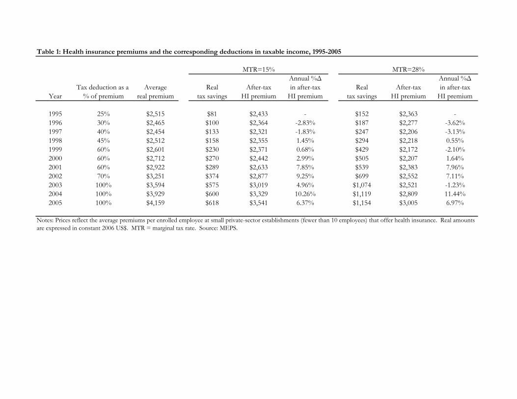
To provide a sense of how these deductions translated into real savings, Table 1

lists the average real individual health insurance premiums and the corresponding after-

tax premiums reflecting the tax savings.3 Information on the average health insurance

premiums are from the 1996-2004 Medical Expenditure Panel Survey-Insurance Compo-

nent (MEPS-IC). Greater detail on the construction of these figures is provided below

in Section 4. For example in 1996, the average real individual health insurance premium

was $2,465. For individuals with a 15 (28) percent MTR, this translated into a real

savings of $100 ($187) when the TRA86-mandated tax deduction equaled 30 percent.

Thus, the after-tax real premium totaled $2,364 ($2,277). By comparison in 2004, the

average real individual health insurance premium rose to $3,929. This translated into

real savings of $600 ($1,119) for individuals with a 15 (28) percent MTR as for the first

time self-employed persons were able to deduct the entire premium from their taxable

income. The corresponding after-tax real premium equaled $3,329 ($2,809). The annual

percentage changes over the entire period reflect that the real premiums rose faster than

the value of the tax deduction. Therefore, the after-tax price of health insurance still

increased for the self-employed during the time period considered.

In order to examine the effects of the TRA86 amendments on the health insurance

coverage of the self-employed, we first utilize a DD approach and follow G&P94 by

comparing the self-employed to wage/salary employees over time. For this purpose, we

use the following regression where the dependent variable, Y , takes on a value of “1” if

individual i in state s was the policyholder of his/her health insurance plan in period t,

and “0” otherwise.

Yits = Xitsα+γSelfEmpits+2005∑

t=1996

δtY earits+2005∑

t=1996

θt(SelfEmpits×Y earits)+Stateitsπs+εits,

(1)

Some individuals may have health insurance coverage from alternative sources, such as

through a spouse’s plan. The TRA86 amendments would not necessarily affect having

any kind of coverage but it is more likely that they provided incentives for the self-

3All real figures are expressed in constant 2006 US$ throughout the text and in the tables.

7

employed to obtain coverage in their own name. Thus, we focus specifically on having

a health insurance plan as the policyholder. By comparison, G&P94 focus on coverage

under a private health insurance plan either in one’s own name or in someone else’s name.

They do this because the CPS questionnaire changed in March 1988 making the survey

responses regarding policyholder status inconsistent over time. X is a vector including

individual and family characteristics as well as a constant term. SelfEmp takes on

a value of “1” if an individual is self-employed, and “0” otherwise (i.e. wage/salary

employee). Y ear is the set of year fixed effects, State is a vector of state fixed effects,

and ε is the error term which we assume is normally distributed. The omitted year is

1995—the year in which the deduction equaled 25 percent, the least generous in the time

frame we analyze.4

The key identifying assumption in estimating our model is that in the absence of

the TRA86 amendments, the unobservable differences between the self-employed (treat-

ment group) and the wage/salary employees (control group) would be the same over

time. In other words, the DD approach provides an unbiased estimate of the effect of

the tax policy change assuming that the unobservable trend factors do not vary across

the groups. Another assumption made in estimating equation (1) is that SelfEmp is

exogenous. Over the time period we analyze, the overall unincorporated self-employment

rate increased from 6.6 percent in 1995 to 7.2 percent in 2005, averaging 7.1 percent for

the entire 10-year period. The figures provided in Tables 2 and 3 lend support for the

aforementioned assumptions.

In Table 2 we exploit the longitudinal feature of the CPS in addressing the possible

endogeneity of any trends in self-employment. The CPS can be used to create a short

panel of two-year cross sections by matching a subsample of individuals between each

consecutive survey year. This subset of the CPS is referred to as the “outgoing rotation

4An alternative specification would be, rather than including each year separately, to constructindicators by grouping together the years in which the TRA86 tax deduction was similar and to interactthem with SelfEmp. For example, we could construct dummies for 1995-1998, 1999-2002, and 2003-2005. Our chosen specification is actually more flexible than this alternative since the DD estimates forany subperiod can be retrieved based on our reported θ̂s.

8

group” (ORG).5 This feature of the CPS provides us with an opportunity to examine the

possible effects of the TRA86 amendments on the year-to-year changes in labor market

status, i.e. between wage/salary employment and self-employment. For this subset of

individuals, we find that the fraction of individuals who switch jobs—from wage/salary

employment into self-employment and vice versa–in any given year is quite small; it is

well under half a percent of our ORG sample. This is likely because the two observations

we have for each individual are only 12 months apart. Only about two percent of the

sample switches over the entire 10-year period.

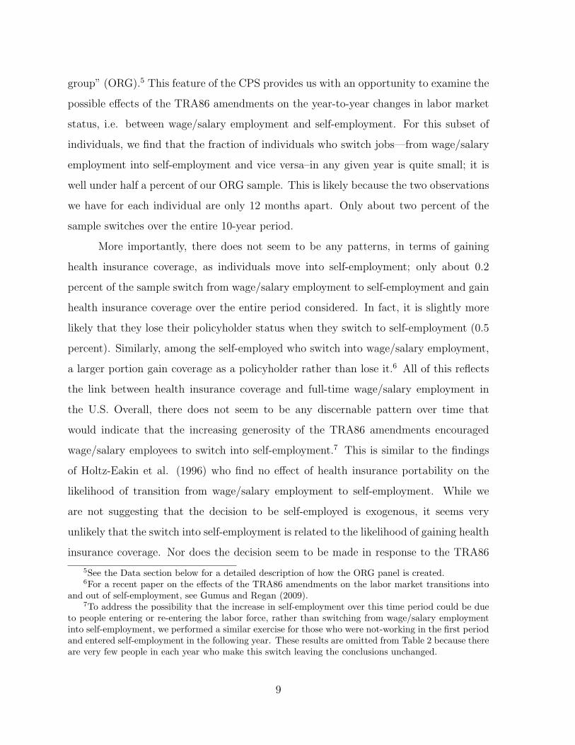
More importantly, there does not seem to be any patterns, in terms of gaining

health insurance coverage, as individuals move into self-employment; only about 0.2

percent of the sample switch from wage/salary employment to self-employment and gain

health insurance coverage over the entire period considered. In fact, it is slightly more

likely that they lose their policyholder status when they switch to self-employment (0.5

percent). Similarly, among the self-employed who switch into wage/salary employment,

a larger portion gain coverage as a policyholder rather than lose it.6 All of this reflects

the link between health insurance coverage and full-time wage/salary employment in

the U.S. Overall, there does not seem to be any discernable pattern over time that

would indicate that the increasing generosity of the TRA86 amendments encouraged

wage/salary employees to switch into self-employment.7 This is similar to the findings

of Holtz-Eakin et al. (1996) who find no effect of health insurance portability on the

likelihood of transition from wage/salary employment to self-employment. While we

are not suggesting that the decision to be self-employed is exogenous, it seems very

unlikely that the switch into self-employment is related to the likelihood of gaining health

insurance coverage. Nor does the decision seem to be made in response to the TRA86

5See the Data section below for a detailed description of how the ORG panel is created.6For a recent paper on the effects of the TRA86 amendments on the labor market transitions into

and out of self-employment, see Gumus and Regan (2009).7To address the possibility that the increase in self-employment over this time period could be due

to people entering or re-entering the labor force, rather than switching from wage/salary employmentinto self-employment, we performed a similar exercise for those who were not-working in the first periodand entered self-employment in the following year. These results are omitted from Table 2 because thereare very few people in each year who make this switch leaving the conclusions unchanged.

9

amendments. The identification of our model does not require that the decision to be

self-employed is orthogonal to the decision to have health insurance coverage. Rather it

simply requires that the respective changes be orthogonal.

Since the ORG panel is short, Table 2 provides limited evidence that the self-

employment trends are independent of changes in health insurance coverage. As a further

test of our assumptions, Table 3 addresses yearly changes in the composition of the

wage/salary and self-employed groups. Considering the period we analyze spans 11

years, it is inevitable that the composition of each of these groups varied over time.

However, our identification strategy only requires that trends in unobservable factors do

not differ such that unbiased DD estimates of the policy change can be obtained. In

what follows, we focus on the trends in the main observable characteristics to determine

if the parallel trends assumption holds. To this end, we perform a separate DD on a

set of covariates to see if the trends in any of the key variables differ in a systematic

way between our treatment (i.e. self-employed) and control (i.e. wage/salaried) groups.

More specifically, we regress each covariate on the set of year dummies, a self-employed

indicator, and the interactions.

Table 3 presents the coefficient estimates of the interaction terms, for both men and

women. In general, there are very few instances in which any of the interaction terms

gain statistical significance. None of these reveal any systematic pattern nor economic

significance that would be of concern; the singular exception is the White indicator

for the sample of women. On the other hand, when we consider the after-tax price of

health insurance there is a clear difference in the trends between the self-employed and

the wage/salaried. The positive and statistically significant coefficient estimates on the

interaction terms reported in the last column of Table 3 are consistent with the numbers

in Table 1. Based on the figures provided in Tables 2 and 3, the possible endogeneity

or composition bias seems quite small and so we proceed with our assumptions. As a

further test of these assumptions, we perform a series of robustness checks that consider

different time periods and use different control groups in the estimations that follow.

These results are reported in Section 4.

10

We use a linear probability model (LPM) to estimate equation (1). Alternatively,

we could estimate equation (1) with a probit or logit model. As discussed in Hotz et al.

(2006), LPMs in DD settings are preferable because they are less computationally intense

and easier to interpret.8 This specification allows us to see how self-employed persons

were affected, relative to wage/salary employees, and to gauge the effects of the increased

generosity of the TRA86 health insurance deductions over time. Hence, the θ̂s are the

DD estimates. The literature (e.g., Perry and Rosen, 2004) has established that the

rate of health insurance coverage is lower for self-employed persons than for wage/salary

individuals. Thus, we expect the γ̂ to be negative. If the TRA86 amendments did in

fact encourage the self-employed to obtain health insurance coverage as a policyholder

over time, we would expect the θ̂s to be positive.

The differences in terms of health insurance coverage between the self-employed

and the wage/salary employees is largely due to the high costs associated with obtaining

health insurance in the private non-group market, although other factors such as differ-

ences in risk attitudes, age, etc. of the self-employed population might be important as

well. In studying the initial TRA86 tax deduction and the demand for health insurance,

G&P94 specify a discrete choice model of individual insurance demand. Based on their

specification we also estimate the following model:

Yits = Xitsφ+ ψSelfEmpits +2005∑

t=1996

ζtY earits + Stateitsηs + λPits + µits, (2)

where Y , X, SelfEmp, Y ear, and State are defined as before and µ is the error term

which is normally distributed. P is a measure of the after-tax premium. We estimate

this model with a LPM as well as with a probit. We conduct the empirical analyses

of equations (1) and (2) separately for men and women. Then, we divide our sample

according to differences in family structure and eligibility. Details on these estimations

8Ai and Norton (2003) discuss the problems associated with estimating the marginal effects for theinteraction terms in non-linear models. They show that in order to correctly estimate the marginal effectof an interaction term, the entire cross-derivative must be calculated. However, there are difficultiesassociated with multiple interaction terms, as in the case of our model.

11

as well as the results are reported in Section 4.

3 Data

The data used in this paper come from the CPS. The CPS is a monthly survey

sponsored by the Census Bureau and the Bureau of Labor Statistics (BLS). Each month

the CPS surveys some 50,000 households (“occupied units”) and is designed to represent

the U.S. civilian, non-institutionalized population.9 Respondents are asked questions

about themselves and persons in the household who are ages 16 and above. The ques-

tions center on demographic characteristics and labor market activities but include other

annual supplementary information as well (e.g., health insurance, tobacco use, computer

ownership). The respondent (“reference person”) is often the owner or renter of the

selected housing unit.

This study uses data from the 1996-2006 CPS surveys. The 1996 survey was the

first year in which detailed questions concerning the source of health insurance coverage

were asked. The analysis for this paper focuses on workers between the ages of 25 and

60. We exclude individuals who were: 1) disabled; 2) full-time students; 3) in the Armed

Forces; as well as those who were 4) unemployed; 5) not in the labor force; and/or 6)

working without pay.10 In our sample, we not only include the respondents but also any

other individual in their family (e.g., spouse) who satisfies the age restriction and the

other criteria mentioned above.

We perform the empirical analysis for men and women separately. In addition, we

divide men and women into further subsamples based on family structure and eligibility

status. Marital status is important in terms of having alternative sources of coverage.11

Single individuals are a special group since they can have coverage only as a policyholder.

Married individuals, on the other hand, may be covered under their spouse’s health

9Beginning in July 2001, the sample size increased to 60,000 occupied households.10Later, in Section 4, we expand the sample to include not-working persons—i.e. individuals in

groups 4, 5, and 6.11Abraham et al. (2006) and Beeson Royalty and Abraham (2006) address the joint nature of the

household demand for health insurance.

12

insurance plan. We further explore the possibility that the presence of children may

reduce the likelihood of self-insuring by considering married persons without children.

Finally, we also address the eligibility restrictions of the TRA86, as noted previously,

by identifying the individuals who are not covered as a dependent under an employer-

provided health insurance plan and whose real annual earnings are at least $2000.

The CPS uses a 4-8-4 sampling scheme meaning that each household is in the survey

for four consecutive months, out for the next eight, and then returns for the following

four months. This survey design creates a longitudinal, albeit short, component called

the “outgoing rotation group” (ORG). Our analysis uses a series of pooled cross-sections

which includes duplicate observations on individuals who are part of the ORG sample.12

About 38 percent of our sample is composed of ORG individuals. The pooled cross-

sections include repeated observations for the ORG respondents and thus we adjust

the standard errors by clustering within individuals in order to correct for the possible

autocorrelation.13 This allows us to maintain the largest sample size and improves the

precision of our estimates.14

The 1996-2006 CPS cross-sectional data correspond to 1995-2005. This is because

the health insurance questions are asked once a year in March and refer to coverage at

any time during the previous calendar year. The CPS contains information on health

insurance coverage from the following sources: 1) a private plan through an employer

(either as a policyholder or dependent); 2) a private plan purchased directly (either

as a policyholder or dependent); 3) a private plan provided by someone outside of the

12In a given survey, individuals are uniquely identified by two variables: a household identifier (HHID)and an individual line number within the household (LINENO). Across surveys, one needs to supplementthese two variables with others in order to match individuals over time. Following Madrian and Lefgren(1999), we use gender, race, age, educational attainment, and foreign birth status to obtain a goodmatch.

13As Moulton (1990), Bertrand et al. (1994), and Donald and Lang (2007) have pointed out, regress-ing individual outcomes on aggregate-level policies (e.g., TRA86) that similarly affect all individuals inone group (e.g., self-employed in a given year) can drastically understate the standard errors of the DDestimates. As it turns out our DD estimates are not statistically significant, thus making the suggestedcorrection redundant. The coefficient estimates would remain unchanged while the standard errorswould be larger.

14The results are robust to eliminating either the first or the second observation on each ORGindividual, thus omitting repeated observations on each individual.

13

household; 4) Medicare; 5) Medicaid; or 6) another type of plan (i.e. state-only plan,

Military Health plan, and Indian Health Service).15 The dependent variable used in our

empirical analysis is whether an individual was covered by a non-public health insurance

plan in their own name in the prior year (i.e. policyholders in categories 1 and 2).

Individuals are considered self-employed if they indicate being self-employed, in terms

of the longest job held within the past year, and if their business was unincorporated.

Since the longest job held corresponds to the prior year, it accords well with the health

insurance variables. This is also consistent with the BLS’ definition of self-employment

(Hipple, 2004).

The controls for individual characteristics used in the analysis include age and its

square. The three race variables are White, Black, and other. The ethnic categories

include Hispanic and other. We include the following levels of completed schooling: high

school graduate, some college, college degree, or an advanced degree. Those with less

than a high school degree are the omitted category. For the family characteristics, we

form the following dummy variables for the number of own-children ages 18 and younger:

having no children (excluded category), one child only, and more than one child. Family

income is defined as the combined income of all family members during the last 12

months. It includes income from jobs, net income from a business/farm/rental unit,

pensions, dividends, interest, social security payments, and any other money income

received by family members ages 15 and above. This measure is adjusted for inflation

and for the number of family members.16

Table 4a (4b) provides the descriptive statistics for men (women) by employment

status. To begin, the sample of working men—both wage/salary and self-employed—is

larger than for women. Self-employed persons are slightly older than their wage/salary

counterparts. A smaller fraction of the self-employed are minorities and fewer of them

report working the typical hours per week (36-55 hours) compared to the wage/salary

employees. While most men are full-time workers, there is a noticeably larger fraction

15Note that these categories are not necessarily mutually exclusive.16Adjusted family income is total family income divided by the square root of the number of family

members.

14

of women who are part-time workers. Since we focus on prime-age working individuals,

the large majority of the sample reports their health status as excellent, very good, or

good. The wage/salary employees and the self-employed are very similar in terms of

their self-reported health status. For both sexes, a larger portion of the wage/salary

employees have some type of health insurance coverage than do the self-employed (83.1

versus 65.8 percent for men and 86.5 versus 75.8 percent for women, respectively). This

difference between the two groups is even more pronounced when one considers only the

policyholders (71.9 versus 39.2 percent for men and 60.2 versus 26.9 percent for women).

The majority of our sample is married, and self-employed people are even more

likely to be so than wage/salary workers. This could be due to the small differences in age

between the two groups. The adjusted family income is higher among the wage/salary

men than the self-employed men which is also partly reflected in the MTRs. Among the

married persons, a larger percentage of men and women in wage/salary employment are

married to spouses who have some source of health insurance coverage but fewer of them

report being married to spouses who are policyholders. In both the wage/salary and

the self-employed samples, it is more common for the women to be married to spouses

with their own employer-provided health insurance plan than it is for men. For example,

among the men in wage/salary employment (self-employment), 37.1 (42.3) percent are

married to spouses who are policy holders of employer-provided health insurance plans,

whereas the corresponding figure for women is 63.6 (62.2) percent. In the next section,

we present the estimation results of our DD and insurance demand models and discuss

some robustness checks.

4 Estimation and Results

Tables 5a and 5b provide the simple sample means and the unadjusted DD esti-

mates for men and women, respectively. Between 1995 and 2005, there are downward

trends in the rate of health insurance coverage as a policyholder. For example in 1995,

70.7 (58.7) percent of all men (women) in our sample had health insurance coverage as a

15

policyholder whereas in 2005 this rate dropped to 65.9 (57.1) percent. Similarly for the

wage/salary men (women), the rates fell from 73.0 (60.4) to 68.6 (59.1) percent. While

the rate of coverage is always higher for wage/salary employees than for self-employed

workers, there are corresponding decreases in the rates of coverage for the self-employed

men and women over time as well. In 1995, 41.1 (28.1) percent of the self-employed

men (women) had coverage under their own name; this figure drops to 34.3 (23.0) per-

cent 10 years later. The simple differences listed in columns 4 and 5 illustrate these

year-to-year changes for each worker-type. The unadjusted DD estimates provided in

the last columns of Tables 5a and 5b reveal the gap in coverage, that is growing over

time, between self-employed persons and wage/salary workers. These DD estimates are

statistically insignificant except for women in 2005. While crude, these figures are some

of the first evidence that the TRA86 amendments did not help in eliminating, nor re-

ducing, the gap in coverage for self-employed persons. Next, we estimate a series of DD

specifications by controlling for a variety of other factors in a regression context.

The estimates of equation (1) can be found in Tables 6a and 6b; the full set of

results are available in Appendix Tables 1a and 1b. Each regression also includes a set

of state-specific effects (not reported) to account for any state-level differences. The

regression results are summarized as follows: Individuals are less likely to have coverage

in their own name if they are self-employed, Black, Hispanic, less educated, younger, a

single man, or a married woman, and have lower family incomes. The DD technique is

performed by comparing self-employed persons to wage/salary workers relative to 1995—

the year in which the TRA86 tax deduction was the least generous (25 percent) during

the time period we analyze.

Table 6a (6b), column 1, provides the estimates of equation (1) for all men (women)

in our sample. Clearly, being self-employed lowers the likelihood that one has a health

insurance plan in his/her name. The negative and statistically significant coefficient es-

timate on this indicator implies that the coverage rates are about 32.6 (30.2) percentage

points lower for self-employed men (women) compared to those in wage/salary employ-

ment. For example, this could be due to differences in risk attitudes between these two

16

groups. The coefficient estimates on the year dummies are almost all negative and gain

statistical significance in the latter years. Jointly, the year dummies are statistically

significant and collectively they suggest that the rate of coverage has declined over time

for both groups; a finding consistent with the figures presented in Tables 5a and 5b. In

contrast, the estimated coefficients on the interaction terms are nearly all negative but

never statistically significant, neither individually nor jointly. The singular exception to

this is for the women; the last interaction term is negative and statistically significant

at the five percent level. Again consistent with the basic DD presented in Tables 5a and

5b, this implies that the TRA86 amendments did not help to close the gap in health

insurance coverage between the self-employed and wage/salary employees. Although the

few statistically significant coefficient estimates suggest that the gap in coverage between

the two groups has grown in size for selected periods, jointly they do not indicate any

economic significance.

Tables 6a and 6b, columns 2-4, restrict the sample by family structure. Column

2 considers single persons. This group is unique in that they do not have any other

possible sources of health insurance coverage from another family member. (Recall that

full-time students and individuals under the age of 25 are omitted from our sample.)

Perhaps due to this lack of alternatives, the gap in health insurance coverage between

the wage/salary employees and the self-employed is smaller for the singles than it was

for the full sample. While smaller in magnitude, the estimated coefficient on SelfEmp

remains statistically significant. In the case of single men (women), the only individual

interaction term that gains statistical significance is negative. So far, we have yet to find

evidence that the gap in coverage has decreased over time as the tax deductions became

more generous. Column 3 considers married persons and column 4 refers to married

persons without children. While health insurance coverage decisions are often made in

the context of the household for married couples, the presence of children presumably

limits the likelihood of self-insuring. Again, the interaction terms remain jointly (and

individually) statistically insignificant for both groups (with the marginal exception of

married women without children in 2005). In sum, redefining our sample according to

17

family structure leaves the results unchanged—the DD estimates show no effect of the

TRA86 amendments.

The TRA86 restricted eligibility to persons with positive net profits who do not

have access to employer-provided health insurance. Unfortunately, the CPS data do not

include information on profits earned. In columns 5 and 6 of Tables 6a and 6b, we use

the same income restriction as in G&P94 and eliminate those persons who earn less

than $2000 per year in real terms. These columns also eliminate anyone who is covered

as a dependent under an employer-provided health insurance plan, although it is not

clear whether this rule is being enforced. We refer to these individuals as “eligible” but

given the limitations of our data we cannot determine with certainty if an individual has

access to employer-provided health insurance.17 Although our eligibility classification

may not be exact, it provides us with an opportunity to investigate this group more

closely. The incentives provided by the tax deductions are greater for these individuals,

holding everything else constant. Restricting our sample in this manner produces some

statistical significance on a limited number of the individual interaction terms, but each

coefficient estimate remains negative. In the case of eligible men (see Table 6a, column 5)

the interaction terms are jointly statistically significant (albeit at the 10 percent level).

However, the DD estimates do not suggest that the gap in coverage is closing over time

as the individual interaction terms, including those that are statistically significant, are

all negative.

Overall the results presented in Tables 6a and 6b are consistent with the unad-

justed DD estimates provided in Tables 5a and 5b. The DD estimates are almost always

statistically insignificant in the regression context (with the exception of eligible men

and married women without children) when we are able to include other controls in the

analysis but the estimated coefficients on the interaction terms are never positive. If

the TRA86 amendments did in fact encourage self-employed persons to obtain cover-

17The reasons for this are: 1) if a spouse reports no employer-provided insurance, it does not neces-sarily imply that he/she was not offered such a plan; and 2) even if a spouse has coverage under sucha plan, we cannot confirm whether the spouse was given the option of including the respondent underthe policy.

18

age, the θ̂s would be positive. Together these findings suggest that the gap between

the wage/salary employees and the self-employed was not reduced by the tax deduc-

tions introduced through the TRA86 amendments. In order to confirm these findings,

we performed two robustness checks. First, we expanded our sample to include those

individuals who were not working. An individual is defined as not-working if he/she is

unemployed, not part of the labor force, or working without pay. As before, we consider

the longest job held within the past year for these classifications. Like the self-employed,

not-working individuals do not have access to employer-provided health insurance. While

both groups purchase their health insurance in the private non-group market, the not-

working group was not eligible for the tax deductions. For this robustness check, we

added a dummy variable for not-working and its interactions with the year dummies.18

Second, we re-estimated our model using 1995-1997 as the omitted reference years instead

of omitting a single year (i.e. 1995). None of these exercises alter the main conclusions

presented above.

Our results so far indicate that there has been no response to the tax deduction.

While the DD analysis is illustrative, it does not account for individual variation in the

after-tax price of health insurance. As G&P94 show, the effect of the policy depends on

the individual’s MTR which was not previously accounted for in our analysis. Next, we

investigate the degree of price elasticity of demand for coverage as a policyholder using

the TRA86 amendments as an identification strategy. This provides a finer measure

of the policy change compared to the DD model because it explicitly accounts for the

rise and the individual variation in the premiums. In order to obtain an estimate of

the price elasticity of demand, we explicitly control for the differences over time in the

after-tax premium of health insurance between the self-employed individuals and the

wage/salary employees. As discussed above, during the period we consider the coverage

rates have been decreasing for both groups. Cutler (2003) studies the reasons for the

decline in health insurance coverage rates in the 1990s despite the economic boom the

18This exercise was only performed only for columns 1-4 of Tables 6a and 6b because we were notable to impose the $2000 earnings threshold for this sample to explore the set of eligibles.

19

U.S. experienced. He finds that the entire decline among the wage/salary employees can

be explained by the increase in employees’ costs of insurance plans.

Wage/salary employees face lower premiums compared to the self-employed not

only because their employers sponsor part of the premium but also because employer-

provided insurance is based on group rates that are substantially below individually

purchased plan rates. G&P94 indicate that while some self-employed might have access

to group insurance coverage, most do not. They calculate the after-tax premium of health

insurance for a single year with data on the distribution of expenditures on health care

and insurance purchased in the non-group market from the 1977 National Medical Care

Expenditure Survey (NMCES). We obtain average individual premium figures using the

Medical Expenditure Panel Survey-Insurance Component (MEPS-IC). The Agency for

Healthcare Research and Quality (AHRQ) make available annual tables from the MEPS-

IC corresponding to 1996-2004 which list the average individual premiums per enrolled

employee at private-sector establishments that offer health insurance.19 The figures are

provided for each state and vary by firm size. For the wage/salary employees, we use

the overall firm averages, by state and by year.

The AHRQ’s MEPS does not have similar information for privately-purchased

non-group plans.20 In fact, obtaining meaningful and reliable average premium figures

for individually purchased plans from any source is nearly impossible. This challenge is

reiterated by Dafny (2008). According to Dafny (2008) the difficulty in obtaining data on

the private health insurance market arises from the complexity of the contracts that are

renegotiated on a yearly basis and are not subject to the usual reporting requirements.

Since no reliable estimates exist, we proxy for the premium of plans purchased in the non-

group market with the MEPS-IC figures corresponding to firms employing less than 10

employees. These premiums reflect the best proxy for what a self-employed individual

19We approximate the figures corresponding to 1995 and 2005 by adjusting the adjacent year’s figurefor the rate of inflation (as measured by the Consumer Price Index)—i.e. between 1995-1996 and2004-2005, respectively.

20MEPS has a Household Component (MEPS-HC) which is a survey of individuals and families.The MEPS-HC asks the respondents, who report having coverage from an individual policy, what theirout-of-pocket premiums are. This is a very small sample and hence cannot provide reliable summarystatistics at the state-level for each year between 1995 and 2005.

20

would face in the market for non-group health insurance. In order to construct an

after-tax figure, we obtain estimated MTRs using the NBER’s TAXSIM program. This

program calculates individuals’ MTRs using information reported on their tax returns

including the tax year, state of residence, marital status, exemptions, various sources

of income (such as wage/salary, dividend, other property, social security, and pensions)

and transfers (such as unemployment compensation and welfare).21 As in G&P94, the

after-tax premium of health insurance, P , is defined as:

P =

I × (1− τ) if wage/salary employee

T × (1−max(β, TRAt)τ) if self-employed,

(3)

where I is the employee’s contribution to his/her health insurance plan and β is the

fraction of the health insurance cost that is claimed as an itemized deduction on one’s

income tax return.22 Individuals (both wage/salary and self-employed) are allowed to

deduct their health insurance premiums from their taxable income as long as the cost,

together with the other eligible medical care expenditures, constitute at least 7.5 percent

of their adjusted gross income (AGI). τ is the individual’s MTR on earned income, and

T is the total health insurance premium which represents both the employee’s and the

employer’s contribution to the health insurance plan. TRAt is the deduction rate allowed

by the TRA86 in each year (e.g., TRA1996 = 0.3).

G&P94 faced additional challenges in estimating the price elasticity of demand

because during the period they analyzed changes other than the partial deductibility

of health insurance premiums by the self-employed occurred. First, the MTRs were

substantially reduced; they note that the top MTR dropped from 50 to 28 percent with

the passage of the TRA86. Second, the amount of permissible medical expenses one

could deduct from their income tax returns was raised from five to 7.5 percent of AGI.

21For more information on TAXSIM, see www.nber.org/taxsim or Feenberg and Coutts (1993).22Note that this may not reflect the true cost of the employer-sponsored plan because of possible

substitution between wages and fringe benefits (Levy, 1998, 2006) and the fact that some employeesworking for small firms do not get to pay for their premiums with pre-tax dollars (Gruber and McKnight,2003).

21

Third, the allowable deduction, for taxpayers who do not itemize, rose sharply from

$3760 to $5000 within a two-year period. It is easier in our case to form a price measure

because our period of analysis is free of other confounding policy changes.

To begin, we estimated equation (2) omitting P . As was the case with the DD

model presented above, the estimated coefficient on SelfEmp is negative and statistically

significant. However, once we include the after-tax health insurance premium in our

regression, ψ̂ is substantially smaller. Table 7 reports only the coefficient estimate on

P and the price semi-elasticity of demand; the full set of results can be found in the

Appendix Tables 2a and 2b.23 The first set of results in Table 7 (M1), corresponding

to the men, report the LPM estimates of equation (2). The coefficient estimates of λs

and their standard errors can be found in the first two rows. λ̂ represents the derivative

of demand with respect to the after-tax price (∂Y∂P

), which is statistically significant at

the one percent level in all specifications. λ̂ is then multiplied by the corresponding cell

average of the after-tax health insurance premium for the self-employed to obtain the

price semi-elasticity which is reported in the third row.24 For example, in (M1) column 1,

the partial derivative of Y with respect to P is -0.107. To obtain the price semi-elasticity

we multiply this figure by 2.955, yielding -0.316. Thus, a one percent decrease in the

after-tax health insurance premium increases the probability that a self-employed man

has coverage as the policyholder by 0.32 percentage points suggesting that this group’s

demand is relatively price inelastic.

Columns 2 and 3 divide the sample into single and married persons. The price semi-

elasticity of demand for single men is larger in magnitude (-0.688) and reveals a greater

degree of price sensitivity compared to those who are married. This finding was expected

since singles lack alternative sources of coverage and hence are more likely to respond to

23This specification explicitly controls for the after-tax price of health insurance, P , unlike the DDmodel. Since P varies by self-employment status, state of residence, year, and MTR, concerns aboutunderstated standard errors are no longer valid (see Donald and Lang, 2007). In estimating equation(2) we no longer regress individual outcomes on aggregate-level policies as was the case for the DD inequation (1).

24Following G&P94, we use the after-tax price for the self-employed since the focus is on theirbehavioral response to the TRA86 and the wage/salary persons merely act as controls for economy-wide events.

22

this particular change in policy. Column 4 corresponds to the set of married individuals

without children and indicates a relatively elastic demand, compared to all married men.

Finally, columns 5 and 6 consider the set of eligible respondents. As expected we see a

greater response to the TRA86 amendments among the eligibles. Further restricting the

sample to include only those eligible persons without children (i.e. column 6) increases

the estimate of the semi-elasticity of demand from -0.415 to -0.597. This again reflects

that the lack of children makes individuals relatively more price sensitive.

The results for the sample of women are provided in Table 7 (W1). Again the λ̂s

are all statistically significant. In addition, they reflect the same order of magnitude as

did the estimates for men. Even the largest estimate of the price semi-elasticity, 1.005

(single women), displays a very limited response to changes in the after-tax price of

health insurance. Thus, for both men and women we see the largest response to the tax

deductions, in terms of estimated price elasticity, by the singles and the eligibles without

children.

Alternatively, we estimated equation (2) with a probit model. The estimates

from this model are found in Table 7, rows (M2) and (W2). Provided here are the

coefficient estimate on P , its derivative (i.e. marginal effect), and the corresponding

price semi-elasticity.25 Overall, these results indicate somewhat smaller estimates of the

price semi-elasticity compared to the figures obtained for LPM. An additional robustness

check is the expansion of our sample to include those individuals who were not-working,

for the reasons mentioned previously. Finally, rather than clustering our standard errors,

we eliminated the duplicate observations corresponding to the persons in the ORG. For

this purpose, we began by eliminating the first observation on each ORG person and

next eliminated the second observation instead. Our conclusions were not altered by

either of these exercises.26

In several instances G&P94 also obtained statistically insignificant responses to

25To calculate the marginal effects reported in Table 7, we evaluate the derivative with respect toprice for each individual observation and take the sample average. We also calculated the marginaleffects using only the self-employed sub-sample and the results are virtually identical.

26The results of these robustness checks are available from the authors upon request.

23

price changes. However, their statistically significant price derivatives yielded larger price

elasticities compared to the ones we estimate. For example, in the case of single men,

they find that a one percent increase in the cost of insurance decreases the probability of

coverage by about 1.8 percentage points. As a final exercise, we attempt to provide an

explanation for these differences. To do this, we re-estimate equation (2) again with an

LPM model but use G&P94’s definition of Y—namely, health insurance coverage as a

policyholder or in someone else’s name (i.e. categories 1, 2, 3 as described in Section 3).

The difference between (M1) and (M3), as well as (W1) and (W3), is relatively larger

for married individuals and negligible for the singles. Our estimates are still smaller

than what G&P94 find and indicate that at least part of the difference stems from the

definition of coverage. By not considering the policyholder status, we along with G&P94

are probably capturing either the response of the individual or possibly that of the spouse

to the policy change without begin able to distinguish between the two.

5 Conclusions

In this paper, we analyze how the tax deductions provided under the TRA86

amendments affected the rates of health insurance coverage among the self-employed.

We find that even the full-deductibility of health insurance premiums was not sufficient

to compensate the self-employed for the high costs associated with obtaining health in-

surance coverage in the private non-group market. Using data from the CPS, correspond-

ing to the period of 1995-2005, we obtain DD estimates comparing the self-employed to

wage/salary employees. These results provide no evidence that the tax deductions were

sufficient to offset the rising premiums during this period. Thus, they did not reduce nor

eliminate the gap in coverage between these two groups. Estimates of the price elasticity

of demand reveal a very limited response to reductions in the after-tax premium. This

conclusion is consistent with earlier findings that the provision of subsidies in the non-

group market is unlikely to generate sizeable reactions among the uninsured (Marquis

and Long, 1995; Gruber, 2005; Gruber and Washington, 2005; Holtz-Eakin, 2005).

24

Former President Bush proposed a series of standard tax deductions aimed at

addressing the nation’s growing uninsured population during his second term in office.

The uninsurance problem gripping America was one of the leading issues in the 2008

Presidential elections. President Obama set forth this issue as one of the priorities

for his administration. His health care plan aims to make insurance affordable and

involves, among his other proposals, subsidies to low- and moderate-income individuals

along with small businesses. While our conclusions pertain only to the self-employed

population and may not generalize to other groups with high rates of uninsurance, our

results do suggest that these types of policies, by themselves, may not provide sufficient

incentives for individuals purchasing health insurance in the private non-group market.

Even when the tax deductions cover a substantial portion of the total premium, obtaining

coverage in this market may still be difficult due to other costs involved (Pauly and

Nichols, 2002; Blumberg and Nichols, 2004). These include, but are not limited to,

search costs, potential denial, and exclusion restrictions on pre-existing conditions. Last

but not least, non-group policies are typically not as generous as the employer-provided

plans in terms of their cost-sharing features (such as co-payments, co-insurance rates,

deductibles) and extent of coverage. Quantifying these other costs is nearly impossible

due to data limitations. And so it seems offering tax deductions alone, without adopting

other policies, may not remedy the uninsurance problem.

Further questions need to be answered to address other relevant issues that are

beyond the scope of the current analysis. For example, how has the non-group health

insurance market been affected by these tax deductions? Were firms encouraged to enter

the market as the tax credits became more generous? How would extending the tax

deductions to other persons, e.g., the not-working, affect the rates of coverage? Would

the tax deductions encourage individuals, who currently have employer-provided health

insurance, to purchase their plans in the non-group market instead? Finally, what other

regulations should be adopted in the non-group market to ensure that the tax deductions

have the intended outcomes? Future research on all of these issues is critical in providing

a more complete answer to the question of whether tax incentives are the solution to the

25

problem of the uninsured.

26

References

[1] Abraham, J.M., W.B. Vogt, M.S. Gaynor, 2006, “How Do Households Choose TheirEmployer-Based Health Insurance?” Inquiry, 43(4), pp. 315-332.

[2] Ai, C. and E.C. Norton, 2003, “Interaction Terms in Logit and Probit Model,”Economic Letters, 80, pp. 123-129.

[3] Beeson Royalty, A. and J.M. Abraham, 2006, “Health Insurance and Labor Mar-ket Outcomes: Joint Decision-Making within Households,” Journal of Public Eco-nomics, 90(8-9), pp. 1561-1577.

[4] Bertrand, M., E. Duflo, and S. Mullainathan, 2004, “How Much Should We TrustDifferences-in-Differences Estimates?”Quarterly Journal of Economics, 119(1), pp.249-275.

[5] Blumberg, L.J. and L.M. Nichols, 2004, “Why are so Many Americans Uninsured?A Conceptual Framework, Summary of the Evidence, and Delineation of the Gapsin our Knowledge,” Health Policy and the Uninsured. C.G. McLaughlin, ed., Wash-ington D.C.; Urban Institute Press, pp. 35-95.

[6] Buchmueller, T.C. and R.G. Valletta, 1996, “The Effects of Employer-ProvidedHealth Insurance on Worker Mobility,” Industrial and Labor Relations Review,49(3), pp. 439-455.

[7] Cutler, D.M., 2003, “Employee Costs and the Decline in Health Insurance Cover-age,” Forum for Health Economics & Policy, 6(3), pp. 1-27.

[8] Dafny, L., 2008, “Are Health Insurance Markets Competitive?,/textquoredblrightNBER Working Paper No.14572.

[9] Donald, S.G. and K. Lang, 2007, “Inference with Difference in Differences and OtherPanel Data,” Review of Economics and Statistics, 89(2), pp. 221-233.

[10] Feenberg, D and E. Coutts. 1993, “An Introduction to the TAXSIM Model,” Journalof Policy Analysis and Management, 12(1), pp. 189-194.

[11] Finkelstein, A., 2002, “The Effect of Tax Subsidies to Employer-Provided Supple-mentary Health Insurance: Evidence from Canada,” Journal of Public Economics,84, pp. 305-339.

[12] Gilleskie, D.B. and B.F. Lutz, 2002, “The Impact of Employer-Provided Health In-surance on Dynamic Employment Transitions,”Journal of Human Resources, 37(1),pp. 129-162.

[13] Gruber, J., 2005, “Tax Policy for Health Insurance,” Tax Policy and the Economy,vol. 19. J. Poterba, ed., Cambridge, MA; MIT Press, pp. 39-63.

27

[14] Gruber, J. and B.C. Madrian, 1994, “Health Insurance and Job Mobility: TheEffects of Public Policy on Job-Lock,” Industrial and Labor Relations Review, 48(1),pp. 86-102.

[15] Gruber, J. and B.C. Madrian, 1997, “Employment Separation and Health InsuranceCoverage,” Journal of Public Economics, 66, pp. 349-382.

[16] Gruber, J. and B.C. Madrian, 2004, “Health Insurance, Labor Supply, and JobMobility: A Critical Review of the Literature,”Health Policy and the Uninsured.C.G. McLaughlin, ed., Washington D.C.; Urban Institute Press.

[17] Gruber, J. and E. Washington, 2005, “Subsidies to Employee Health InsurancePremiums and the Health Insurance Market,”Journal of Health Economics, 24(2),pp. 253-276.

[18] Gruber, J. and J. Poterba, 1994, “Tax Incentives and the Decision to PurchaseHealth Insurance: Evidence from the Self-Employed,” Quarterly Journal of Eco-nomics, 109, pp. 701-733.

[19] Gruber, J. and R. McKnight, 2003, “Why Did Employee Health Insurance Contri-butions Rise,” Journal of Health Economics, 22(6), pp. 1085-1104. 109, pp. 701-733.

[20] Gumus, G. and T.L. Regan, 2009, “Self-Employment and the Role of Health Insur-ance,” IZA Discussion Paper No. 3952.

[21] Heim, B.T. and I.Z. Lurie, 2007, “Do Increased Premium Subsidies Affect HowMuch Health Insurance Is Purchased? Evidence from the Self-Employed,” WorkingPaper.

[22] Hipple, S., 2004, “Self-Employment in the United States: An Update,” MonthlyLabor Review, 127(7), pp. 13-23.

[23] Holtz-Eakin, D., 2005, “The Price Sensitivity of Demand for Nongroup Health In-surance,” Congressional Budget Office Background Paper.

[24] Holtz-Eakin, D., J.R. Penrod, and H.S. Rosen, 1996, “Health Insurance and theSupply of Entrepreneurs,” Journal of Public Economics, 62, pp. 209-235.

[25] Hotz, J.V., C.H. Mullin, and J.K. Scholz, 2006, “Examining the Effect of the EarnedIncome Tax Credit on the Labor Market Participation of Families on Welfare,”NBER Working Paper, No. 11968.

[26] Kaiser Commission on Medicaid and the Uninsured, 2005, “Health Insurance Cov-erage in America: 2005 Data Update.”

[27] Levy, H., 1998, “Why Pays for Health Insurance? Employee Contributions to HealthInsurance Premiums,” Working Paper.

28

[28] Levy, H., 2006, “Health Insurance and the Wage Gap,” NBER Working Paper No.11975.

[29] Lyke, Bob, 2005. “Tax Benefits for Health Insurance and Expenses: Current Legis-lation,” Congressional Research Service Issue Brief for Congress, IB98037.

[30] Madrian, B.C., 1994, “Employment-Based Health Insurance and Job Mobility: IsThere Evidence of Job-Lock?” Quarterly Journal of Economics, 109, pp. 27-54.

[31] Madrian, B.C., 2006, “The U.S. Health Care System and Labor Markets,” NBERWorking Paper, No. 11980.

[32] Madrian, B.C. and L.J. Lefgren, 1999, “A Note on Longitudinally Matching CurrentPopulation Survey (CPS) Respondents,” NBER Technical Working Paper, No. 247.

[33] Marquis, M.S. and S.H. Long, 1995, “Worker Demand for Health Insurance in theNongroup Market,” Journal of Health Economics, 14(1), pp. 47-63.

[34] Meer, J. and H.S. Rosen, 2002, “Insurance, Health, and the Utilization of MedicalServices,” CEPS Working Paper, No. 85.

[35] Moulton, B.R., 1990, “An Illustration of a Pitfall in Estimating the Effects of Ag-gregate Variables on Micro Units,”Review of Economics and Statistics, 72(2), pp.334-338.

[36] Pauly, M.V. and L.M. Nichols, 2002, “The Nongroup Health Insurance Market:Short on Facts, Long on Opinions and Policy Disputes,” Health Affairs Web Exclu-sive, W325-W344.

[37] Perry, C. W. and H.S. Rosen, 2004, “The Self-Employed are Less Likely than WageEarners to Have Health Insurance than Wage-Earners. So What?” Public Policy andthe Economics of Entrepreneurship. D. Holtz-Eakin and H. Rosen, ed., Cambridge,MA; MIT Press pp. 23-58.

[38] Thomasson, M., 2002, “From Sickness to Health: The Twentieth-Century Develop-ment of U.S. Health Insurance,” Explorations in Economic History, 39, pp. 233-253.

[39] Thomasson, M., 2003, “The Importance of Group Coverage: How Tax PolicyShaped U.S. Health Insurance,” American Economic Review, 93, pp. 1373-1384.

29

Annual %Δ Annual %ΔTax deduction as a Average Real After-tax in after-tax Real After-tax in after-tax

Year % of premium real premium tax savings HI premium HI premium tax savings HI premium HI premium

1995 25% $2,515 $81 $2,433 - $152 $2,363 -1996 30% $2,465 $100 $2,364 -2.83% $187 $2,277 -3.62%1997 40% $2,454 $133 $2,321 -1.83% $247 $2,206 -3.13%1998 45% $2,512 $158 $2,355 1.45% $294 $2,218 0.55%1999 60% $2,601 $230 $2,371 0.68% $429 $2,172 -2.10%2000 60% $2,712 $270 $2,442 2.99% $505 $2,207 1.64%2001 60% $2,922 $289 $2,633 7.85% $539 $2,383 7.96%2002 70% $3,251 $374 $2,877 9.25% $699 $2,552 7.11%2003 100% $3,594 $575 $3,019 4.96% $1,074 $2,521 -1.23%2004 100% $3,929 $600 $3,329 10.26% $1,119 $2,809 11.44%2005 100% $4,159 $618 $3,541 6.37% $1,154 $3,005 6.97%

MTR=28%

Table 1: Health insurance premiums and the corresponding deductions in taxable income, 1995-2005

are expressed in constant 2006 US$. MTR = marginal tax rate. Source: MEPS.

MTR=15%

Notes: Prices reflect the average premiums per enrolled employee at small private-sector establishments (fewer than 10 employees) that offer health insurance. Real amounts

gain HI policy lose HI policy gain HI policy lose HI policy Year holder status holder status holder status holder status

1995 414 (0.21%) 0.02% 0.04% 438 (0.22%) 0.04% 0.03%

1996 613 (0.31%) 0.03% 0.06% 306 (0.15%) 0.03% 0.02%

1997 393 (0.20%) 0.02% 0.04% 423 (0.21%) 0.04% 0.02%

1998 371 (0.19%) 0.02% 0.04% 394 (0.20%) 0.04% 0.01%

1999 393 (0.20%) 0.02% 0.05% 395 (0.20%) 0.04% 0.02%

2000 371 (0.19%) 0.02% 0.04% 387 (0.19%) 0.05% 0.01%

2001 491 (0.25%) 0.02% 0.07% 519 (0.26%) 0.06% 0.03%

2002 470 (0.24%) 0.02% 0.05% 511 (0.26%) 0.05% 0.02%

2003 456 (0.23%) 0.02% 0.06% 417 (0.21%) 0.04% 0.02%

2004 464 (0.23%) 0.02% 0.04% 484 (0.24%) 0.05% 0.02%

All years 4,436 (2.23%) 0.19% 0.50% 4,274 (2.15%) 0.43% 0.20%

Number of switchers

Previously self-employed% of switchers who

to self-employment (%) to wage/salary (%)

Notes: †The figures correspond to the men and women in the outgoing rotation group (ORG) only (N=199,161).

Table 2: Health insurance (HI) policy holder status among switchers†

Previously wage/salary% of switchers who

Number of switchers

Years of Number of Adjusted+ After-tax++

Covariate Age White Black Hispanic schooling Excellent Very good Good Fair Poor Married children family income price of HI

Self-emp × 1996 0.020 -0.004 -0.005 -0.002 0.192 0.017 -0.004 -0.001 -0.014 0.001 -0.019 -0.026 0.463** -0.011Self-emp × 1997 0.543 0.005 -0.010 -0.010 0.225* 0.008 -0.014 0.011 -0.011 0.005 -0.001 -0.076 0.208 -0.081**Self-emp × 1998 0.179 -0.001 -0.006 -0.004 0.085 0.023 -0.017 0.002 -0.009 0.001 -0.010 -0.047 0.039 -0.014Self-emp × 1999 0.252 -0.002 -0.008 -0.010 0.181 0.001 0.006 0.009 -0.018* 0.002 -0.015 -0.071 -0.055 0.032**Self-emp × 2000 0.507 0.001 -0.012 -0.024** 0.102 0.002 -0.008 0.015 -0.009 0.000 -0.015 -0.062 -0.082 0.314**Self-emp × 2001 0.371 0.002 0.000 -0.009 0.031 -0.006 0.002 0.009 -0.010 0.004 -0.015 -0.044 -0.422** 0.491**Self-emp × 2002 0.494 -0.005 0.012 -0.001 -0.166 -0.022 -0.004 0.034* -0.008 -0.000 -0.011 -0.040 -0.314 0.650**Self-emp × 2003 0.562 0.005 -0.002 0.000 -0.107 -0.006 -0.006 0.017 -0.007 0.003 -0.030 -0.073 -0.185 0.741**Self-emp × 2004 0.209 -0.006 0.004 -0.002 -0.145 -0.016 0.000 0.016 -0.005 0.004 -0.039* -0.128** -0.459** 0.759**Self-emp × 2005 0.556 -0.010 0.006 0.001 -0.010 -0.013 0.008 0.008 -0.006 0.003 -0.039* -0.114** 0.080 0.719**

Years of Number of Adjusted+ After-tax++

Covariate Age White Black Hispanic schooling Excellent Very good Good Fair Poor Married children family income price of HI

Self-emp × 1996 -0.769* -0.010 0.000 -0.006 0.175 0.037 -0.008 -0.039* 0.003 0.008 -0.016 0.043 0.346 -0.008Self-emp × 1997 -0.135 -0.017 0.002 -0.008 0.048 0.027 -0.010 -0.019 0.002 0.000 0.000 -0.030 0.185 -0.073**Self-emp × 1998 -0.012 -0.015 0.009 -0.000 0.219 0.053* -0.033 -0.031 0.012 -0.001 0.004 -0.007 0.351 -0.005Self-emp × 1999 -0.144 -0.029* 0.023 -0.005 0.014 0.022 0.006 -0.025 -0.007 0.004 0.026 -0.017 0.054 0.037*Self-emp × 2000 0.332 -0.020 0.003 -0.014 0.017 0.005 -0.016 0.006 0.001 0.005 0.019 -0.082 0.440* 0.345**Self-emp × 2001 -0.223 -0.027* 0.016 -0.002 0.072 0.026 -0.029 -0.005 0.002 0.005 -0.007 -0.019 -0.013 0.475**Self-emp × 2002 -0.123 -0.030* 0.009 -0.002 -0.023 0.009 -0.009 -0.001 -0.001 0.002 0.000 -0.017 -0.062 0.661**Self-emp × 2003 -0.137 -0.037** 0.022* -0.000 0.033 0.004 -0.016 -0.013 0.020* 0.005 -0.014 -0.032 -0.258 0.774**Self-emp × 2004 -0.393 -0.029* 0.020* -0.004 0.143 0.050* -0.026 -0.023 -0.006 0.005 -0.022 -0.020 -0.089 0.723**Self-emp × 2005 -0.474 -0.032* 0.006 0.003 0.048 0.032 -0.001 -0.028 -0.004 0.001 -0.006 -0.024 -0.138 0.714**

construction of the after-tax health insurance premiums. * Significance at 5%. ** Significance at 1%.

Notes: All models are based on weighted and clustered data and they include a constant term, self-employed indicator, and year effects. Excluded categories are year 1995 and itsinteraction with the self-employed indicator. + Family income is adjusted for the household size and expressed in constant 2006 US$. ++ See Section 4 for the details on the

Health status

Table 3: Difference-in-difference for selected covariates, men and women

MEN (N=377,454)

WOMEN (N=348,203)Health status

Mean St. Error Mean St. ErrorIndividual characteristicsAge 40.731 0.023 43.785 0.073

Age 25-34 0.307 0.001 0.189 0.003Age 35-44 0.330 0.001 0.330 0.004Age 45-54 0.264 0.001 0.329 0.004Age 55-60 0.098 0.001 0.153 0.003

Race/EthnicityWhite 0.841 0.001 0.890 0.002Black 0.102 0.001 0.054 0.002

Hispanic 0.127 0.001 0.092 0.002Education

Years of schooling 13.499 0.007 13.439 0.023Less than high school 0.101 0.001 0.108 0.002

High school degree 0.323 0.001 0.354 0.004Some college degree 0.261 0.001 0.251 0.003

Bachelor's degree 0.207 0.001 0.179 0.003Graduate degree 0.107 0.001 0.108 0.002

Weekly hours worked1-20 0.017 0.000 0.052 0.002

21-35 0.047 0.000 0.122 0.00236-55 0.839 0.001 0.625 0.004

55+ 0.097 0.001 0.200 0.003Health status

Excellent 0.350 0.001 0.338 0.003Very good 0.367 0.001 0.361 0.003

Good 0.234 0.001 0.242 0.003Fair 0.043 0.000 0.050 0.002

Poor 0.006 0.000 0.008 0.001Health insurance

Any 0.831 0.001 0.658 0.004Policy holder 0.719 0.001 0.392 0.004

Family characteristicsMarried 0.669 0.001 0.709 0.004Number of children under age 18 0.826 0.003 0.852 0.009

No children 0.563 0.001 0.565 0.004One child 0.171 0.001 0.166 0.003

More than one child 0.266 0.001 0.269 0.003Adjusted family income ($10,000)+ 4.825 0.010 4.399 0.036Estimated marginal tax rate (MTR)*

MTR = 0 0.053 0.000 0.127 0.0020 < MTR ≤ 10 0.035 0.000 0.051 0.002

10 < MTR ≤ 15 0.426 0.001 0.402 0.00315 < MTR ≤ 28 0.362 0.001 0.284 0.003

MTR > 28 0.124 0.001 0.135 0.002

Spouse characteristics †

Spouse has any health insurance (HI) coverage 0.892 0.001 0.778 0.004Spouse is HI policy holder 0.391 0.001 0.503 0.004Spouse is policy holder of an emp.-provided HI 0.371 0.001 0.423 0.004

N

conditional on being married.

Table 4a: Descriptive statistics, men

346,513 30,941

Self-employedWage/salary

Notes: Means and standard errors are based on weighted and clustered data. + Family income is adjusted for the household sizeand expressed in constant 2006 US$. * MTR are estimated using the TAXSIM program. † Means for spouse characteristics are

Mean St. Error Mean St. ErrorIndividual characteristicsAge 41.021 0.024 43.108 0.090

Age 25-34 0.296 0.001 0.203 0.004Age 35-44 0.327 0.001 0.351 0.005Age 45-54 0.277 0.001 0.313 0.004Age 55-60 0.100 0.001 0.133 0.003

Race/EthnicityWhite 0.811 0.001 0.881 0.003Black 0.134 0.001 0.059 0.002

Hispanic 0.100 0.001 0.072 0.002Education

Years of schooling 13.652 0.006 13.759 0.025Less than high school 0.071 0.001 0.067 0.002

High school degree 0.317 0.001 0.301 0.004Some college degree 0.299 0.001 0.316 0.005

Bachelor's degree 0.213 0.001 0.210 0.004Graduate degree 0.099 0.001 0.106 0.003

Weekly hours worked1-20 0.090 0.001 0.258 0.004

21-35 0.155 0.001 0.212 0.00436-55 0.722 0.001 0.430 0.005

55+ 0.033 0.000 0.100 0.003Health status

Excellent 0.325 0.001 0.365 0.004Very good 0.369 0.001 0.354 0.004

Good 0.249 0.001 0.223 0.004Fair 0.051 0.000 0.048 0.002

Poor 0.007 0.000 0.009 0.001Health insurance

Any 0.865 0.001 0.758 0.004Policy holder 0.602 0.001 0.269 0.004

Family characteristicsMarried 0.626 0.001 0.746 0.004Number of children under age 18 0.850 0.003 0.987 0.011

No children 0.529 0.001 0.498 0.005One child 0.204 0.001 0.177 0.003

More than one child 0.267 0.001 0.324 0.004Adjusted family income ($10,000)+ 4.588 0.010 4.607 0.045Estimated marginal tax rate (MTR)*

MTR = 0 0.092 0.001 0.143 0.0030 ≤ MTR ≤ 10 0.036 0.000 0.045 0.0020 ≤ MTR ≤ 15 0.424 0.001 0.398 0.0040 ≤ MTR ≤ 28 0.345 0.001 0.280 0.004

MTR > 28 0.102 0.001 0.134 0.003

Spouse characteristics †

Spouse has any health insurance (HI) coverage 0.913 0.001 0.860 0.004Spouse is HI policy holder 0.670 0.001 0.752 0.005Spouse is policy holder of an emp.-provided HI 0.636 0.001 0.622 0.005

N

conditional on being married. and expressed in constant 2006 US$. * MTR are estimated using the TAXSIM program. † Means for spouse characteristics are

Table 4b: Descriptive statistics, women

327,951 20,252

Self-employedWage/salary

Notes: Means and standard errors are based on weighted and clustered data. + Family income is adjusted for the household size

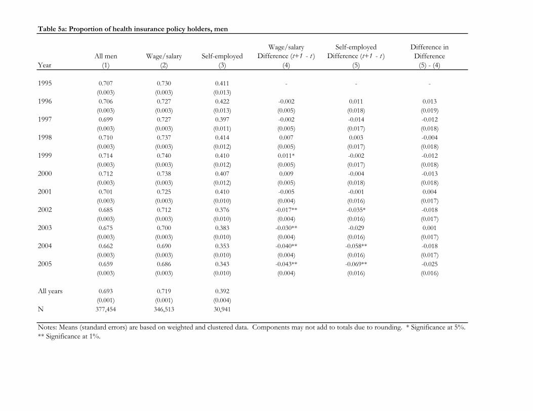
Wage/salary Self-employed Difference inAll men Wage/salary Self-employed Difference (t+1 - t ) Difference (t+1 - t ) Difference

Year (1) (2) (3) (4) (5) (5) - (4)

1995 0.707 0.730 0.411 - - -(0.003) (0.003) (0.013)

1996 0.706 0.727 0.422 -0.002 0.011 0.013(0.003) (0.003) (0.013) (0.005) (0.018) (0.019)

1997 0.699 0.727 0.397 -0.002 -0.014 -0.012(0.003) (0.003) (0.011) (0.005) (0.017) (0.018)

1998 0.710 0.737 0.414 0.007 0.003 -0.004(0.003) (0.003) (0.012) (0.005) (0.017) (0.018)

1999 0.714 0.740 0.410 0.011* -0.002 -0.012(0.003) (0.003) (0.012) (0.005) (0.017) (0.018)

2000 0.712 0.738 0.407 0.009 -0.004 -0.013(0.003) (0.003) (0.012) (0.005) (0.018) (0.018)

2001 0.701 0.725 0.410 -0.005 -0.001 0.004(0.003) (0.003) (0.010) (0.004) (0.016) (0.017)

2002 0.685 0.712 0.376 -0.017** -0.035* -0.018(0.003) (0.003) (0.010) (0.004) (0.016) (0.017)

2003 0.675 0.700 0.383 -0.030** -0.029 0.001(0.003) (0.003) (0.010) (0.004) (0.016) (0.017)

2004 0.662 0.690 0.353 -0.040** -0.058** -0.018(0.003) (0.003) (0.010) (0.004) (0.016) (0.017)

2005 0.659 0.686 0.343 -0.043** -0.069** -0.025(0.003) (0.003) (0.010) (0.004) (0.016) (0.016)

All years 0.693 0.719 0.392(0.001) (0.001) (0.004)

N 377,454 346,513 30,941

Notes: Means (standard errors) are based on weighted and clustered data. Components may not add to totals due to rounding. * Significance at 5%.

Table 5a: Proportion of health insurance policy holders, men

** Significance at 1%.

Wage/salary Self-employed Difference inAll women Wage/salary Self-employed Difference (t+1 - t ) Difference (t+1 - t ) Difference

Year (1) (2) (3) (4) (5) (5) - (4)

1995 0.587 0.604 0.281 - - -(0.004) (0.004) (0.014)

1996 0.590 0.605 0.277 0.001 -0.004 -0.005(0.004) (0.004) (0.015) (0.005) (0.020) (0.021)

1997 0.585 0.605 0.263 0.001 -0.018 -0.019(0.003) (0.004) (0.013) (0.005) (0.019) (0.020)

1998 0.585 0.604 0.281 0.000 0.001 0.001(0.003) (0.004) (0.013) (0.005) (0.019) (0.020)

1999 0.580 0.598 0.279 -0.006 -0.002 0.004(0.003) (0.004) (0.014) (0.005) (0.020) (0.020)

2000 0.588 0.608 0.267 0.004 -0.014 -0.018(0.004) (0.004) (0.013) (0.005) (0.019) (0.020)

2001 0.589 0.607 0.272 0.003 -0.008 -0.011(0.003) (0.003) (0.011) (0.005) (0.018) (0.018)

2002 0.581 0.600 0.260 -0.004 -0.021 -0.017(0.003) (0.003) (0.011) (0.005) (0.018) (0.018)

2003 0.581 0.599 0.272 -0.005 -0.009 -0.004(0.003) (0.003) (0.011) (0.005) (0.018) (0.019)

2004 0.580 0.598 0.282 -0.006 0.002 0.008(0.003) (0.003) (0.012) (0.005) (0.018) (0.019)

2005 0.571 0.591 0.230 -0.013** -0.051** -0.038*(0.003) (0.003) (0.011) (0.005) (0.017) (0.018)

All years 0.583 0.602 0.269(0.001) (0.001) (0.004)

N 348,203 327,951 20,252

Notes: Means (standard errors) are based on weighted and clustered data. Components may not add to totals due to rounding. * Significance at 5%.

Table 5b: Proportion of health insurance policy holders, women

** Significance at 1%.

Married men Eligible menVariable All men Single men Married men without kids Eligible men without kids

(1) (2) (3) (4) (5) (6)Self-employed -0.326** -0.260** -0.355** -0.375** -0.275** -0.260**

(0.013) (0.025) (0.015) (0.023) (0.015) (0.021)1996 -0.002 0.006 -0.007 -0.010 0.002 0.000

(0.004) (0.008) (0.005) (0.007) (0.004) (0.006)1997 -0.005 0.010 -0.013* -0.014 0.002 0.002

(0.004) (0.008) (0.005) (0.008) (0.004) (0.006)1998 -0.000 0.014 -0.007 -0.009 0.001 0.001

(0.004) (0.008) (0.005) (0.008) (0.004) (0.006)1999 0.002 0.019* -0.007 -0.013 0.007 0.005

(0.004) (0.008) (0.005) (0.008) (0.004) (0.006)2000 -0.002 0.026** -0.014** -0.020* 0.006 0.007

(0.004) (0.008) (0.005) (0.008) (0.004) (0.006)2001 -0.015** 0.008 -0.025** -0.031** -0.008 -0.008

(0.004) (0.008) (0.005) (0.007) (0.004) (0.006)2002 -0.026** -0.016* -0.029** -0.040** -0.017** -0.023**

(0.004) (0.008) (0.005) (0.008) (0.004) (0.006)2003 -0.038** -0.024** -0.043** -0.046** -0.028** -0.030**

(0.004) (0.008) (0.005) (0.008) (0.004) (0.006)2004 -0.046** -0.029** -0.052** -0.064** -0.034** -0.036**

(0.004) (0.008) (0.005) (0.008) (0.004) (0.006)2005 -0.048** -0.032** -0.054** -0.069** -0.037** -0.042**

(0.004) (0.008) (0.005) (0.008) (0.004) (0.006)Self-emp × 1996 0.005 -0.007 0.011 0.053 -0.007 -0.003

(0.017) (0.033) (0.019) (0.030) (0.020) (0.028)Self-emp × 1997 -0.022 -0.038 -0.015 0.015 -0.018 -0.015

(0.017) (0.033) (0.020) (0.031) (0.020) (0.027)Self-emp × 1998 -0.011 -0.028 -0.002 0.021 -0.013 -0.015

(0.017) (0.033) (0.020) (0.031) (0.020) (0.027)Self-emp × 1999 -0.020 -0.043 -0.008 0.034 -0.022 -0.022

(0.017) (0.033) (0.020) (0.032) (0.020) (0.027)Self-emp × 2000 -0.022 -0.055 -0.009 0.009 -0.028 -0.046

(0.017) (0.034) (0.020) (0.032) (0.021) (0.028)Self-emp × 2001 0.002 0.007 -0.000 0.006 -0.000 -0.013

(0.016) (0.032) (0.019) (0.031) (0.019) (0.027)Self-emp × 2002 -0.011 -0.005 -0.012 0.002 -0.039* -0.045

(0.016) (0.031) (0.018) (0.030) (0.019) (0.027)Self-emp × 2003 0.001 -0.035 0.013 0.037 -0.022 -0.037

(0.016) (0.031) (0.019) (0.031) (0.019) (0.027)Self-emp × 2004 -0.014 -0.043 -0.004 0.047 -0.025 -0.027

(0.016) (0.031) (0.018) (0.030) (0.019) (0.026)Self-emp × 2005 -0.030 -0.061* -0.022 -0.005 -0.053** -0.068**

(0.016) (0.031) (0.018) (0.030) (0.019) (0.026)Joint significance (p-values)

Year dummies 0.000 0.000 0.000 0.000 0.000 0.000Interaction terms 0.288 0.272 0.652 0.419 0.093 0.178

Year DVs & interactions 0.000 0.000 0.000 0.000 0.000 0.000R2 0.124 0.149 0.116 0.106 0.179 0.157N 377,454 108,132 269,322 95,292 307,777 160,749

Table 6a: Difference-in-difference regression results, men

Notes: All models include individual and family characteristics, a constant term, and state effects. For full regression results, see AppendixTable 1a. Excluded categories are non-Hispanic whites, less than high school degree, no children, year 1995, and its interaction with theself-employed indicator. Standard errors are in parantheses. * Significance at 5%. ** Significance at 1%.

Married women Eligible womenVariable All women Single women Married women without kids Eligible women without kids

(1) (2) (3) (4) (5) (6)Self-employed -0.302** -0.241** -0.322** -0.320** -0.323** -0.281**

(0.013) (0.030) (0.015) (0.026) (0.021) (0.029)1996 -0.001 0.009 -0.008 -0.012 0.001 -0.002

(0.004) (0.007) (0.006) (0.009) (0.005) (0.006)1997 -0.005 -0.002 -0.006 -0.017 -0.007 -0.014*

(0.005) (0.007) (0.006) (0.009) (0.005) (0.006)1998 -0.010* -0.004 -0.012 -0.025** -0.010* -0.018**

(0.005) (0.007) (0.006) (0.009) (0.005) (0.006)1999 -0.017** 0.006 -0.030** -0.031** -0.008 -0.013*

(0.005) (0.007) (0.006) (0.009) (0.005) (0.006)2000 -0.011* 0.009 -0.021** -0.027** -0.006 -0.017**

(0.005) (0.007) (0.006) (0.010) (0.005) (0.006)2001 -0.014** -0.002 -0.022** -0.038** -0.010* -0.021**

(0.004) (0.007) (0.006) (0.009) (0.005) (0.006)2002 -0.023** -0.013 -0.029** -0.038** -0.022** -0.031**

(0.004) (0.007) (0.006) (0.009) (0.005) (0.006)2003 -0.027** -0.024** -0.027** -0.035** -0.032** -0.038**

(0.004) (0.007) (0.006) (0.009) (0.005) (0.006)2004 -0.029** -0.023** -0.030** -0.042** -0.032** -0.039**

(0.004) (0.007) (0.006) (0.009) (0.005) (0.006)2005 -0.039** -0.043** -0.035** -0.046** -0.044** -0.051**

(0.004) (0.007) (0.006) (0.009) (0.005) (0.006)Self-emp × 1996 -0.010 -0.048 0.006 -0.011 0.001 -0.028

(0.019) (0.040) (0.021) (0.037) (0.030) (0.041)Self-emp × 1997 -0.024 -0.052 -0.016 -0.010 -0.048 -0.047

(0.018) (0.040) (0.021) (0.035) (0.029) (0.039)Self-emp × 1998 -0.006 -0.025 0.002 0.001 -0.019 -0.029

(0.018) (0.041) (0.020) (0.035) (0.029) (0.038)Self-emp × 1999 0.008 -0.018 0.025 0.013 0.004 0.008

(0.019) (0.043) (0.021) (0.035) (0.029) (0.040)Self-emp × 2000 -0.022 -0.053 -0.007 -0.006 -0.033 -0.034

(0.019) (0.042) (0.021) (0.035) (0.030) (0.040)Self-emp × 2001 -0.016 -0.044 -0.004 -0.020 -0.033 -0.060

(0.017) (0.038) (0.019) (0.033) (0.027) (0.037)Self-emp × 2002 -0.014 -0.076* 0.009 0.005 -0.033 -0.049

(0.017) (0.038) (0.019) (0.034) (0.027) (0.038)Self-emp × 2003 -0.007 -0.069 0.018 0.005 -0.039 -0.075*

(0.018) (0.038) (0.020) (0.034) (0.027) (0.037)Self-emp × 2004 0.000 -0.021 0.009 -0.014 -0.006 -0.033

(0.018) (0.038) (0.019) (0.034) (0.027) (0.037)Self-emp × 2005 -0.038* -0.065 -0.030 -0.080* -0.046 -0.094*

(0.017) (0.038) (0.019) (0.032) (0.027) (0.038)Joint significance (p-values)

Year dummies 0.000 0.000 0.000 0.000 0.000 0.000Interaction terms 0.227 0.577 0.142 0.112 0.373 0.195

Year DVs & interactions 0.000 0.000 0.000 0.000 0.000 0.000R2 0.120 0.161 0.074 0.056 0.130 0.097N 348,203 122,196 226,007 89,356 236,374 127,934

Table 6b: Difference-in-difference regression results, women

Notes: All models include individual and family characteristics, a constant term, and state effects. For full regression results, see AppendixTable 1b. Excluded categories are non-Hispanic whites, less than high school degree, no children, year 1995, and its interaction with theself-employed indicator. Standard errors are in parantheses. * Significance at 5%. ** Significance at 1%.

Married men Eligible menMEN All men Single men Married men without kids Eligible men without kids

(1) (2) (3) (4) (5) (6)(M1) Health insurance/Policy holder (LPM)

Coefficient -0.107** -0.228** -0.050** -0.085** -0.142** -0.204**(0.006) (0.011) (0.007) (0.012) (0.007) (0.010)

Semi-elasticity -0.316 -0.688 -0.147 -0.250 -0.415 -0.597(M2) Health insurance/Policy holder (Probit)

Coefficient -0.301** -0.640** -0.135** -0.218** -0.363** -0.540**(0.018) (0.039) (0.021) (0.036) (0.023) (0.033)

Marginal effect -0.095** -0.205** -0.042** -0.067** -0.094** -0.149**Semi-elasticity -0.281 -0.618 -0.123 -0.197 -0.275 -0.436

(M3) Health insurance/Gruber & Poterba measure (LPM)Coefficient -0.147** -0.224** -0.097** -0.164** -0.148** -0.207**

(0.006) (0.011) (0.007) (0.011) (0.007) (0.010)Semi-elasticity -0.434 -0.676 -0.285 -0.483 -0.433 -0.606

N 377,454 108,132 269,322 95,292 307,777 160,749

Married women Eligible womenWOMEN All women Single women Married women without kids Eligible women without kids

(1) (2) (3) (4) (5) (6)(W1) Health insurance/Policy holder (LPM)

Coefficient -0.136** -0.321** -0.024** -0.047** -0.238** -0.245**(0.007) (0.014) (0.008) (0.014) (0.010) (0.014)

Semi-elasticity -0.404 -1.005 -0.070 -0.138 -0.710 -0.726(W2) Health insurance/Policy holder (Probit)

Coefficient -0.443** -0.900** -0.082** -0.147** -0.684** -0.683**(0.024) (0.055) (0.028) (0.043) (0.033) (0.045)

Marginal effect -0.156** -0.269** -0.031** -0.055** -0.204** -0.191**Semi-elasticity -0.464 -0.843 -0.091 -0.162 -0.609 -0.566

(W3) Health insurance/Gruber & Poterba measure (LPM)Coefficient -0.210** -0.304** -0.101** -0.145** -0.232** -0.223**

(0.007) (0.014) (0.008) (0.013) (0.009) (0.013)Semi-elasticity -0.625 -0.952 -0.295 -0.427 -0.692 -0.661

N 348,203 122,196 226,007 89,356 236,374 127,934

Notes: All models include individual and family characteristics, a constant term, and state effects. For full regression results, see Appendix Tables 2a and 2b. Standard errors

Table 7: Estimates of insurance demand, men and women

are in parantheses. * Significance at 5%. ** Significance at 1%.

Married men Eligible menVariable All men Single men Married men without kids Eligible men without kids

(1) (2) (3) (4) (5) (6)Self-employed -0.326** -0.260** -0.355** -0.375** -0.275** -0.260**

(0.013) (0.025) (0.015) (0.023) (0.015) (0.021)1996 -0.002 0.006 -0.007 -0.010 0.002 0.000

(0.004) (0.008) (0.005) (0.007) (0.004) (0.006)1997 -0.005 0.010 -0.013* -0.014 0.002 0.002

(0.004) (0.008) (0.005) (0.008) (0.004) (0.006)1998 -0.000 0.014 -0.007 -0.009 0.001 0.001

(0.004) (0.008) (0.005) (0.008) (0.004) (0.006)1999 0.002 0.019* -0.007 -0.013 0.007 0.005

(0.004) (0.008) (0.005) (0.008) (0.004) (0.006)2000 -0.002 0.026** -0.014** -0.020* 0.006 0.007

(0.004) (0.008) (0.005) (0.008) (0.004) (0.006)2001 -0.015** 0.008 -0.025** -0.031** -0.008 -0.008

(0.004) (0.008) (0.005) (0.007) (0.004) (0.006)2002 -0.026** -0.016* -0.029** -0.040** -0.017** -0.023**

(0.004) (0.008) (0.005) (0.008) (0.004) (0.006)2003 -0.038** -0.024** -0.043** -0.046** -0.028** -0.030**

(0.004) (0.008) (0.005) (0.008) (0.004) (0.006)2004 -0.046** -0.029** -0.052** -0.064** -0.034** -0.036**

(0.004) (0.008) (0.005) (0.008) (0.004) (0.006)2005 -0.048** -0.032** -0.054** -0.069** -0.037** -0.042**

(0.004) (0.008) (0.005) (0.008) (0.004) (0.006)Self-emp × 1996 0.005 -0.007 0.011 0.053 -0.007 -0.003

(0.017) (0.033) (0.019) (0.030) (0.020) (0.028)Self-emp × 1997 -0.022 -0.038 -0.015 0.015 -0.018 -0.015

(0.017) (0.033) (0.020) (0.031) (0.020) (0.027)Self-emp × 1998 -0.011 -0.028 -0.002 0.021 -0.013 -0.015

(0.017) (0.033) (0.020) (0.031) (0.020) (0.027)Self-emp × 1999 -0.020 -0.043 -0.008 0.034 -0.022 -0.022

(0.017) (0.033) (0.020) (0.032) (0.020) (0.027)Self-emp × 2000 -0.022 -0.055 -0.009 0.009 -0.028 -0.046

(0.017) (0.034) (0.020) (0.032) (0.021) (0.028)Self-emp × 2001 0.002 0.007 -0.000 0.006 -0.000 -0.013

(0.016) (0.032) (0.019) (0.031) (0.019) (0.027)Self-emp × 2002 -0.011 -0.005 -0.012 0.002 -0.039* -0.045

(0.016) (0.031) (0.018) (0.030) (0.019) (0.027)Self-emp × 2003 0.001 -0.035 0.013 0.037 -0.022 -0.037

(0.016) (0.031) (0.019) (0.031) (0.019) (0.027)Self-emp × 2004 -0.014 -0.043 -0.004 0.047 -0.025 -0.027

(0.016) (0.031) (0.018) (0.030) (0.019) (0.026)Self-emp × 2005 -0.030 -0.061* -0.022 -0.005 -0.053** -0.068**

(0.016) (0.031) (0.018) (0.030) (0.019) (0.026)Age 0.012** 0.016** 0.008** 0.001 0.017** 0.013**

(0.001) (0.002) (0.001) (0.002) (0.001) (0.001)Age squared/100 -0.010** -0.013** -0.005** 0.003 -0.016** -0.011**

(0.001) (0.002) (0.001) (0.002) (0.001) (0.001)Black -0.067** -0.063** -0.062** -0.049** -0.064** -0.059**

(0.004) (0.006) (0.005) (0.007) (0.004) (0.005)Hispanic -0.127** -0.124** -0.130** -0.137** -0.142** -0.126**

(0.003) (0.005) (0.004) (0.006) (0.003) (0.005)

Appendix Table 1a: Full set of estimation results for the difference-in-difference regression model, men

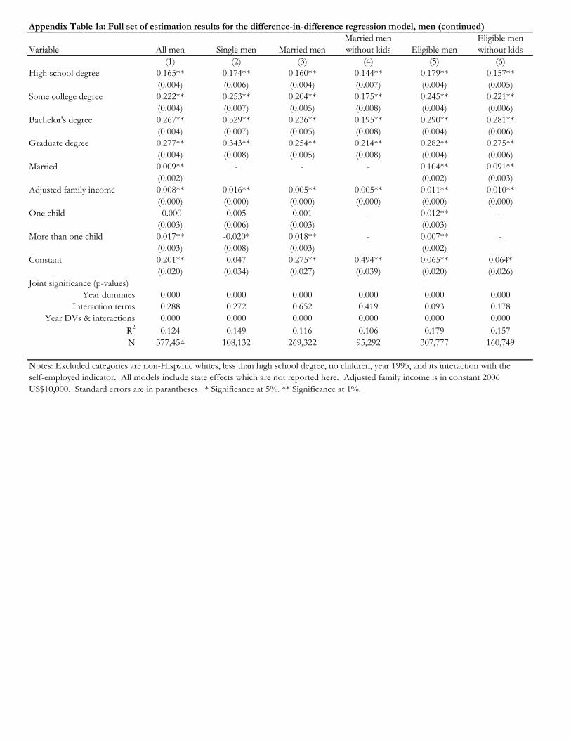
Married men Eligible menVariable All men Single men Married men without kids Eligible men without kids

(1) (2) (3) (4) (5) (6)High school degree 0.165** 0.174** 0.160** 0.144** 0.179** 0.157**

(0.004) (0.006) (0.004) (0.007) (0.004) (0.005)Some college degree 0.222** 0.253** 0.204** 0.175** 0.245** 0.221**

(0.004) (0.007) (0.005) (0.008) (0.004) (0.006)Bachelor's degree 0.267** 0.329** 0.236** 0.195** 0.290** 0.281**

(0.004) (0.007) (0.005) (0.008) (0.004) (0.006)Graduate degree 0.277** 0.343** 0.254** 0.214** 0.282** 0.275**

(0.004) (0.008) (0.005) (0.008) (0.004) (0.006)Married 0.009** - - - 0.104** 0.091**

(0.002) (0.002) (0.003)Adjusted family income 0.008** 0.016** 0.005** 0.005** 0.011** 0.010**

(0.000) (0.000) (0.000) (0.000) (0.000) (0.000)One child -0.000 0.005 0.001 - 0.012** -

(0.003) (0.006) (0.003) (0.003)More than one child 0.017** -0.020* 0.018** - 0.007** -

(0.003) (0.008) (0.003) (0.002)Constant 0.201** 0.047 0.275** 0.494** 0.065** 0.064*

(0.020) (0.034) (0.027) (0.039) (0.020) (0.026)Joint significance (p-values)

Year dummies 0.000 0.000 0.000 0.000 0.000 0.000Interaction terms 0.288 0.272 0.652 0.419 0.093 0.178

Year DVs & interactions 0.000 0.000 0.000 0.000 0.000 0.000R2 0.124 0.149 0.116 0.106 0.179 0.157N 377,454 108,132 269,322 95,292 307,777 160,749

US$10,000. Standard errors are in parantheses. * Significance at 5%. ** Significance at 1%.self-employed indicator. All models include state effects which are not reported here. Adjusted family income is in constant 2006

Appendix Table 1a: Full set of estimation results for the difference-in-difference regression model, men (continued)

Notes: Excluded categories are non-Hispanic whites, less than high school degree, no children, year 1995, and its interaction with the

Married women Eligible womenVariable All women Single women Married women without kids Eligible women without kids

(1) (2) (3) (4) (5) (6)Self-employed -0.302** -0.241** -0.322** -0.320** -0.323** -0.281**

(0.013) (0.030) (0.015) (0.026) (0.021) (0.029)1996 -0.001 0.009 -0.008 -0.012 0.001 -0.002

(0.004) (0.007) (0.006) (0.009) (0.005) (0.006)1997 -0.005 -0.002 -0.006 -0.017 -0.007 -0.014*

(0.005) (0.007) (0.006) (0.009) (0.005) (0.006)1998 -0.010* -0.004 -0.012 -0.025** -0.010* -0.018**

(0.005) (0.007) (0.006) (0.009) (0.005) (0.006)1999 -0.017** 0.006 -0.030** -0.031** -0.008 -0.013*

(0.005) (0.007) (0.006) (0.009) (0.005) (0.006)2000 -0.011* 0.009 -0.021** -0.027** -0.006 -0.017**

(0.005) (0.007) (0.006) (0.010) (0.005) (0.006)2001 -0.014** -0.002 -0.022** -0.038** -0.010* -0.021**

(0.004) (0.007) (0.006) (0.009) (0.005) (0.006)2002 -0.023** -0.013 -0.029** -0.038** -0.022** -0.031**

(0.004) (0.007) (0.006) (0.009) (0.005) (0.006)2003 -0.027** -0.024** -0.027** -0.035** -0.032** -0.038**

(0.004) (0.007) (0.006) (0.009) (0.005) (0.006)2004 -0.029** -0.023** -0.030** -0.042** -0.032** -0.039**

(0.004) (0.007) (0.006) (0.009) (0.005) (0.006)2005 -0.039** -0.043** -0.035** -0.046** -0.044** -0.051**

(0.004) (0.007) (0.006) (0.009) (0.005) (0.006)Self-emp × 1996 -0.010 -0.048 0.006 -0.011 0.001 -0.028

(0.019) (0.040) (0.021) (0.037) (0.030) (0.041)Self-emp × 1997 -0.024 -0.052 -0.016 -0.010 -0.048 -0.047

(0.018) (0.040) (0.021) (0.035) (0.029) (0.039)Self-emp × 1998 -0.006 -0.025 0.002 0.001 -0.019 -0.029

(0.018) (0.041) (0.020) (0.035) (0.029) (0.038)Self-emp × 1999 0.008 -0.018 0.025 0.013 0.004 0.008

(0.019) (0.043) (0.021) (0.035) (0.029) (0.040)Self-emp × 2000 -0.022 -0.053 -0.007 -0.006 -0.033 -0.034

(0.019) (0.042) (0.021) (0.035) (0.030) (0.040)Self-emp × 2001 -0.016 -0.044 -0.004 -0.020 -0.033 -0.060

(0.017) (0.038) (0.019) (0.033) (0.027) (0.037)Self-emp × 2002 -0.014 -0.076* 0.009 0.005 -0.033 -0.049

(0.017) (0.038) (0.019) (0.034) (0.027) (0.038)Self-emp × 2003 -0.007 -0.069 0.018 0.005 -0.039 -0.075*

(0.018) (0.038) (0.020) (0.034) (0.027) (0.037)Self-emp × 2004 0.000 -0.021 0.009 -0.014 -0.006 -0.033

(0.018) (0.038) (0.019) (0.034) (0.027) (0.037)Self-emp × 2005 -0.038* -0.065 -0.030 -0.080* -0.046 -0.094*

(0.017) (0.038) (0.019) (0.032) (0.027) (0.038)Age 0.008** 0.016** -0.000 -0.006** 0.017** 0.012**

(0.001) (0.001) (0.001) (0.002) (0.001) (0.001)Age squared/100 -0.006** -0.012** 0.001 0.007** -0.016** -0.010**

(0.001) (0.002) (0.002) (0.002) (0.001) (0.001)Black 0.014** -0.027** 0.066** 0.050** -0.031** -0.029**

(0.003) (0.004) (0.005) (0.008) (0.003) (0.004)Hispanic -0.046** -0.084** -0.028** -0.058** -0.091** -0.092**

(0.003) (0.005) (0.004) (0.007) (0.004) (0.005)

Appendix Table 1b: Full set of estimation results for the difference-in-difference regression model, women

Married women Eligible womenVariable All women Single women Married women without kids Eligible women without kids

(1) (2) (3) (4) (5) (6)High school degree 0.153** 0.208** 0.107** 0.087** 0.198** 0.168**

(0.004) (0.006) (0.006) (0.009) (0.005) (0.007)Some college degree 0.208** 0.284** 0.147** 0.132** 0.271** 0.230**

(0.004) (0.006) (0.006) (0.009) (0.005) (0.007)Bachelor's degree 0.272** 0.359** 0.204** 0.185** 0.338** 0.292**

(0.005) (0.007) (0.006) (0.010) (0.005) (0.007)Graduate degree 0.334** 0.371** 0.287** 0.271** 0.364** 0.323**

(0.005) (0.007) (0.007) (0.011) (0.005) (0.007)Married -0.179** - - - -0.002 -0.033**

(0.002) (0.002) (0.003)Adjusted family income 0.006** 0.022** 0.003** 0.001** 0.012** 0.010**

(0.000) (0.001) (0.000) (0.000) (0.000) (0.000)One child -0.065** -0.034** -0.075** - -0.019** -

(0.003) (0.004) (0.004) (0.003)More than one child -0.137** -0.098** -0.151** - -0.070** -

(0.003) (0.005) (0.004) (0.003)Constant 0.281** 0.031 0.464** 0.572** 0.017 0.166**

(0.022) (0.031) (0.032) (0.046) (0.023) (0.029)Joint significance (p-values)

Year dummies 0.000 0.000 0.000 0.000 0.000 0.000Interaction terms 0.227 0.577 0.142 0.112 0.373 0.195

Year DVs & interactions 0.000 0.000 0.000 0.000 0.000 0.000R2 0.120 0.161 0.074 0.056 0.130 0.097N 348,203 122,196 226,007 89,356 236,374 127,934

US$10,000. Standard errors are in parantheses. * Significance at 5%. ** Significance at 1%.self-employed indicator. All models include state effects which are not reported here. Adjusted family income is in constant 2006

Appendix Table 1b: Full set of estimation results for the difference-in-difference regression model, women (continued)

Notes: Excluded categories are non-Hispanic whites, less than high school degree, no children, year 1995, and its interaction with the

Married men Eligible menVariable Single men Married men without kids Eligible men without kids

(0) (1) (2) (3) (4) (5) (6)Self-employed -0.338** -0.074** 0.284** -0.239** -0.145** 0.050** 0.213**

(0.004) (0.015) (0.029) (0.018) (0.032) (0.018) (0.026)1996 -0.002 -0.002 0.005 -0.007 -0.006 0.001 0.000

(0.004) (0.004) (0.008) (0.004) (0.007) (0.004) (0.006)1997 -0.007 -0.011* -0.001 -0.016** -0.016* -0.004 -0.006

(0.004) (0.004) (0.008) (0.005) (0.008) (0.004) (0.006)1998 -0.001 0.002 0.018* -0.006 -0.005 0.004 0.005

(0.004) (0.004) (0.008) (0.005) (0.008) (0.004) (0.006)1999 0.001 0.006 0.028** -0.005 -0.005 0.013** 0.014*

(0.004) (0.004) (0.008) (0.005) (0.008) (0.004) (0.006)2000 -0.003 0.006 0.041** -0.011* -0.012 0.016** 0.020**

(0.004) (0.004) (0.008) (0.005) (0.008) (0.004) (0.006)2001 -0.014** 0.001 0.041** -0.018** -0.018* 0.012** 0.019**

(0.004) (0.004) (0.008) (0.005) (0.007) (0.004) (0.006)2002 -0.026** -0.005 0.029** -0.021** -0.023** 0.007 0.013*

(0.004) (0.004) (0.008) (0.005) (0.008) (0.004) (0.006)2003 -0.038** -0.011** 0.028** -0.029** -0.022** 0.004 0.015*

(0.004) (0.004) (0.008) (0.005) (0.008) (0.004) (0.006)2004 -0.047** -0.016** 0.034** -0.038** -0.035** 0.003 0.018**

(0.004) (0.004) (0.008) (0.005) (0.008) (0.004) (0.006)2005 -0.050** -0.021** 0.026** -0.042** -0.045** -0.003 0.008

(0.004) (0.004) (0.008) (0.005) (0.008) (0.004) (0.006)Age 0.012** 0.012** 0.015** 0.007** 0.001 0.016** 0.013**

(0.001) (0.001) (0.002) (0.001) (0.002) (0.001) (0.001)Age squared/100 -0.010** -0.010** -0.012** -0.005** 0.003 -0.015** -0.010**

(0.001) (0.001) (0.002) (0.001) (0.002) (0.001) (0.001)Black -0.067** -0.066** -0.061** -0.062** -0.048** -0.063** -0.058**

(0.004) (0.004) (0.006) (0.005) (0.007) (0.004) (0.005)Hispanic -0.127** -0.126** -0.123** -0.130** -0.136** -0.141** -0.125**

(0.003) (0.003) (0.005) (0.004) (0.006) (0.003) (0.005)High school degree 0.165** 0.163** 0.171** 0.159** 0.143** 0.177** 0.155**

(0.004) (0.004) (0.006) (0.004) (0.007) (0.004) (0.005)Some college degree 0.222** 0.220** 0.248** 0.204** 0.173** 0.243** 0.217**

(0.004) (0.004) (0.007) (0.005) (0.008) (0.004) (0.006)Bachelor's degree 0.267** 0.264** 0.323** 0.235** 0.193** 0.287** 0.276**

(0.004) (0.004) (0.007) (0.005) (0.008) (0.004) (0.006)Graduate degree 0.277** 0.274** 0.335** 0.253** 0.212** 0.278** 0.269**

(0.004) (0.004) (0.008) (0.005) (0.008) (0.004) (0.006)Married 0.009** 0.009** - - - 0.103** 0.091**

(0.002) (0.002) (0.002) (0.003)Adjusted family income 0.008** 0.007** 0.014** 0.005** 0.005** 0.010** 0.009**

(0.000) (0.000) (0.000) (0.000) (0.000) (0.000) (0.000)One child -0.000 -0.001 0.006 0.000 - 0.011** -

(0.003) (0.003) (0.006) (0.003) (0.003)More than one child 0.017** 0.015** -0.015 0.017** - 0.005* -

(0.003) (0.003) (0.008) (0.003) (0.002)After-tax HI premium - -0.107** -0.228** -0.050** -0.085** -0.142** -0.204**

(0.006) (0.011) (0.007) (0.012) (0.007) (0.010)Constant 0.202** 0.250** 0.143** 0.297** 0.525** 0.126** 0.143**

(0.020) (0.021) (0.034) (0.027) (0.039) (0.020) (0.027)R2 0.124 0.125 0.155 0.116 0.107 0.181 0.161N 377,454 377,454 108,132 269,322 95,292 307,777 160,749

After-tax HI premium is in constant 2006 US$1,000. Standard errors are in parantheses. * Significance at 5%. ** Significance at 1%.

Appendix Table 2a: Full set of estimation results for the health insurance demand regression (LPM), men

employed indicator. All models include state effects which are not reported here. Adjusted family income is in constant 2006 US$10,000.Notes: Excluded categories are non-Hispanic whites, less than high school degree, no children, year 1995, and its interaction with the self-

All men

Married women Eligible womenVariable Single women Married women without kids Eligible women without kids

(0) (1) (2) (3) (4) (5) (6)Self-employed -0.314** 0.021 0.545** -0.262** -0.215** 0.241** 0.284**

(0.004) (0.018) (0.037) (0.020) (0.036) (0.025) (0.035)1996 -0.002 -0.001 0.007 -0.008 -0.013 0.001 -0.003

(0.004) (0.004) (0.007) (0.005) (0.008) (0.005) (0.006)1997 -0.006 -0.010* -0.014* -0.008 -0.019* -0.017** -0.024**

(0.005) (0.005) (0.007) (0.006) (0.009) (0.005) (0.006)1998 -0.010* -0.006 0.005 -0.011 -0.024** -0.004 -0.013*

(0.005) (0.005) (0.007) (0.006) (0.009) (0.005) (0.006)1999 -0.016** -0.009 0.025** -0.027** -0.028** 0.005 -0.000

(0.005) (0.005) (0.007) (0.006) (0.009) (0.005) (0.006)2000 -0.012* -0.000 0.034** -0.019** -0.023* 0.012* -0.000

(0.005) (0.005) (0.007) (0.006) (0.009) (0.005) (0.006)2001 -0.015** 0.004 0.041** -0.019** -0.033** 0.020** 0.009

(0.004) (0.004) (0.007) (0.006) (0.009) (0.005) (0.006)2002 -0.024** 0.001 0.044** -0.024** -0.029** 0.020** 0.011

(0.004) (0.004) (0.007) (0.006) (0.009) (0.005) (0.006)2003 -0.027** 0.005 0.048** -0.020** -0.024* 0.020** 0.013

(0.004) (0.005) (0.007) (0.006) (0.009) (0.005) (0.007)2004 -0.029** 0.008 0.063** -0.023** -0.030** 0.030** 0.023**

(0.004) (0.005) (0.007) (0.006) (0.010) (0.005) (0.007)2005 -0.041** -0.005 0.040** -0.031** -0.039** 0.015** 0.007

(0.004) (0.005) (0.008) (0.006) (0.010) (0.005) (0.007)Age 0.008** 0.007** 0.014** -0.000 -0.006** 0.016** 0.011**

(0.001) (0.001) (0.001) (0.001) (0.002) (0.001) (0.001)Age squared/100 -0.006** -0.006** -0.011** 0.001 0.007** -0.015** -0.009**

(0.001) (0.001) (0.002) (0.002) (0.002) (0.001) (0.001)Black 0.014** 0.014** -0.026** 0.066** 0.050** -0.030** -0.029**

(0.003) (0.003) (0.004) (0.005) (0.008) (0.003) (0.004)Hispanic -0.046** -0.046** -0.082** -0.028** -0.057** -0.090** -0.091**

(0.003) (0.003) (0.005) (0.004) (0.007) (0.004) (0.005)High school degree 0.153** 0.151** 0.202** 0.107** 0.086** 0.195** 0.164**

(0.004) (0.004) (0.006) (0.006) (0.009) (0.005) (0.007)Some college degree 0.208** 0.205** 0.275** 0.147** 0.131** 0.266** 0.225**

(0.004) (0.004) (0.006) (0.006) (0.009) (0.005) (0.007)Bachelor's degree 0.272** 0.268** 0.346** 0.203** 0.184** 0.330** 0.284**

(0.005) (0.005) (0.007) (0.006) (0.010) (0.005) (0.007)Graduate degree 0.334** 0.330** 0.357** 0.287** 0.270** 0.356** 0.315**

(0.005) (0.005) (0.007) (0.007) (0.011) (0.005) (0.007)Married -0.179** -0.182** - - - -0.006* -0.033**

(0.002) (0.002) (0.002) (0.003)Adjusted family income 0.006** 0.005** 0.019** 0.003** 0.001* 0.010** 0.009**

(0.000) (0.000) (0.001) (0.000) (0.000) (0.000) (0.000)One child -0.065** -0.065** -0.031** -0.075** - -0.019** -

(0.003) (0.003) (0.004) (0.004) (0.003)More than one child -0.137** -0.138** -0.088** -0.152** - -0.069** -

(0.003) (0.003) (0.005) (0.004) (0.003)After-tax HI premium - -0.136** -0.321** -0.024** -0.047** -0.238** -0.245**

(0.007) (0.014) (0.008) (0.014) (0.010) (0.014)Constant 0.282** 0.346** 0.185** 0.475** 0.591** 0.131** 0.268**

(0.022) (0.022) (0.031) (0.032) (0.046) (0.024) (0.030)R2 0.119 0.121 0.169 0.073 0.056 0.134 0.101N 348,203 348,203 122,196 226,007 89,356 236,374 127,934

After-tax HI premium is in constant 2006 US$1,000. Standard errors are in parantheses. * Significance at 5%. ** Significance at 1%.

Appendix Table 2b: Full set of estimation results for the health insurance demand regression (LPM), women

employed indicator. All models include state effects which are not reported here. Adjusted family income is in constant 2006 US$10,000.Notes: Excluded categories are non-Hispanic whites, less than high school degree, no children, year 1995, and its interaction with the self-

All women