PDViPeR DocumentationRelease 1.2

Australian Synchrotron

February 25, 2016

Contents

1 Contents: 31.1 General Information . . . . . . . . . . . . . . . . . . . . . . . . . . . . . . . . . . . . . . . . . . . 31.2 Installation . . . . . . . . . . . . . . . . . . . . . . . . . . . . . . . . . . . . . . . . . . . . . . . . 31.3 How to use PDViPeR . . . . . . . . . . . . . . . . . . . . . . . . . . . . . . . . . . . . . . . . . . . 61.4 Future development . . . . . . . . . . . . . . . . . . . . . . . . . . . . . . . . . . . . . . . . . . . 161.5 About PDViPeR . . . . . . . . . . . . . . . . . . . . . . . . . . . . . . . . . . . . . . . . . . . . . 161.6 .parab and .xy/.xye file formats . . . . . . . . . . . . . . . . . . . . . . . . . . . . . . . . . . . . . 17

2 Modules 192.1 processing . . . . . . . . . . . . . . . . . . . . . . . . . . . . . . . . . . . . . . . . . . . . . . . . 19

3 Indices and tables 21

i

ii

PDViPeR Documentation, Release 1.2

PDViPeR 1 is a data analysis program developed for use on the Australian Synchrotron (AS) Powder Diffraction(PD) beamline. It takes data captured on the Mythen microstrip detector and performs the following post-processingoperations:

• Reads .xye and .xy ASCII columnar data files and writes processed files in .xye format

• Visual comparison of datasets.

• Aligns and merges dataset pairs based on a user-specified alignment region.

• Two merge methods (splice and merge) with normalisation to a specified detector position or reference file.

• Outputs plots suitable for publication or editing: Vertically stacked series, interpolated 2D image and 3D water-fall plots.

• X-axis/abscissa rescaling between 2𝜃, d-space and Q units.

1 PDViPeR – Powder Diffraction Visualisation Processing and Reporting.

Contents 1

PDViPeR Documentation, Release 1.2

2 Contents

CHAPTER 1

Contents:

1.1 General Information

PDViPeR is a BSD-licensed data visualisation, processing and reporting software package for powder diffraction data.PDViPeR is a python-based package that not only reads in, views, and plots Australian Synchrotron Powder Diffractionbeamline data, but also is capable of efficient multi-detector position data merging that has been performed admirablyin the past by DataPro and other programs. The package is capable of easily producing images for publication andreports, with a range of output options including raw, stack, 2D surface and 3D plots. Dataset normalisation, scaling,background subtraction and inputting of both XYE and XY file formats are additional features. The goal of theapplication is to create an integrated package that will enable Users of the Powder Diffraction beamline to view,process and display their data easily and efficiently for publication.

1.2 Installation

PDViPeR is written in Python (2.7 at the time of writing) and has several module dependencies that require installation.For Windows users, there is a self-contained installation package file available as the recommended download optionfor PDViPeR that does not require the dependencies to be installed separately. It can be downloaded from the PDViPeRdownload page

For Linux and Mac users the easiest way to install these dependencies is to install one of the Enthought PythonDistributions. The EPDFree distribution contains all the modules on which PDViPeR depends. A typical user can justdownload and install EPDFree then download and unpack PDViPeR and run it immediately.

Some users might prefer alternatives to EPDFree. For example Academic or Commercial users may prefer to use one ofEnthought’s other distributions. Other popular Python distributions include Python(x,y), WinPython and ActiveState’sActivePython, all of which will require installation of at least some of the following dependencies:

1.2.1 Python package dependencies

PDViPeR depends on the following Python modules being installed in the Python environment

• numpy

• scipy

• matplotlib

• traits [part of the Enthought Tool Suite (ETS) package]

• traitsui (part of ETS)

3

PDViPeR Documentation, Release 1.2

• chaco (part of ETS)

• pyface (part of ETS)

• wxPython

Those wishing to build the documentation from source will also need Sphinx. For those familiar with installingPython packages, the dependencies can be found in the central repository of Python modules. For Microsoft Windowsusers, Christoph Gohlke (C.G.) maintains a useful repository of Windows installers for many modules. Linux userscan typically find the dependencies using their package manager (e.g. synaptic or yum). Mac users should visit theindividual sites linked above for instructions.

1.2.2 Example 1. Windows installation using the self-contained executable file (rec-ommended)

1. Visit the PDViPeR download page and select the latest version of the Windows Installer. To install PDViPeRdouble click the downloaded executable file and follow the step-by-step instructions

1.2.3 Example 2. Windows installation using Enthought Python Distribution (rec-ommended)

1. Visit the PDViPeR download page and follow the instructions to obtain the EPD Free Python installer and thePDViPeR installer files for Windows. You may wish to visit the Enthought website, directly, and choose one ofEnthought’s other Python distributions. Note, EPD Free satisfies the dependencies listed above.

2. Run the epd_free-*.msi installer to install EPD Free.

3. Verify that Python is running correctly. e.g. for Windows 7, click on Start Menu|AllPrograms|Accessories|Command Prompt. At the > prompt type python -c "print ’helloworld’" noting single and double quotes. Verify that hello world is displayed.

4. Running the PDViPeR installer will install PDViPeR and create a start menu entry.

1.2.4 Example 3. Windows installation using Python(x,y) (optional)

1. Visit the Python(x,y) downloads page and install a distribution.

2. Verify that Python is running correctly (see Example 1. Windows installation using the self-contained executablefile (recommended)).

3. Visit the PDViPeR download page and follow the instructions to obtain the PDViPeR setup file.

4. Running the installer will install PDViPeR and create a start menu entry.

1.2.5 Example 4. Windows installation on a system with Python already installed(experienced)

Note: untested.

1. Check the package dependency list above.

2. The easiest way here is to use the packages provided by Python(x,y) and/or Christoph Gohlke. Install therequired dependency, taking care to choose packages for Python 2.7 and to choose the 32 or 64 bit package ver-sion that matches your Python version. Install in turn numpy (if in doubt choose the numpy-MKL-... version),scipy, matplotlib, wxPython, and finally ETS.

4 Chapter 1. Contents:

PDViPeR Documentation, Release 1.2

1.2.6 Example 5. Linux installation using Enthought Python Distribution (recom-mended)

1. Visit the PDViPeR download page and follow the instructions to obtain the EPD Free Python installer and thePDViPeR .zip package for Linux. You may wish to visit the Enthought website, directly, and choose one ofEnthought’s other Python distributions. Note, EPD Free satisfies the dependencies listed above.

2. Run the epd_free-*.sh shell script to install EPD Free.

3. Verify that Python is running correctly. e.g. for Ubuntu, open a terminal. At the $ prompt type python -c"print ’hello world’" noting single and double quotes. Verify that hello world is displayed.

4. The main PDViPeR application file is app.py in the directory into which PDViPeR was unpacked.

5. PDViPeR can be started by running ./start_pdviper.sh or ./app.py. To do this, at the $ prompt typechmod 777 start_pdviper.sh app.py followed by, for example, ./start_pdviper.sh

1.2.7 Example 6. Linux installation using synaptic (experienced)

Note: untested.

This description is for Ubuntu Linux. yum packaged names in Fedora Linux flavours should have similar names.

1. First, verify that Python2.7 is running correctly. e.g. for Ubuntu, open a terminal. At the $ prompt type python-c "import sys; print sys.version". Verify that a string displays identifying a 2.7 branch versionof Python.

2. Using synaptic or apt-get install <package> install the following packages: python-numpy,python-scipy, python-matplotlib, python-traits, python-traitsui, python-chaco,python-pyface, python-wxgtk2.8

3. Visit the PDViPeR download page and follow the instructions to obtain the package.

4. The main application file is app.py in the directory into which PDViPeR was unpacked.

5. PDViPeR can be started by running ./start_pdviper.sh or ./app.py. To do this, at the $ prompt typechmod 777 start_pdviper.sh app.py followed by, for example, ./start_pdviper.sh

1.2.8 Example 7. Mac OSX installation (recommended)

1. Visit the PDViPeR download page and follow the instructions to obtain the EPD Free Python installer and thePDViPeR .zip package for Mac OSX. You may wish to visit the Enthought website, directly, and choose one ofEnthought’s other Python distributions. Note, EPD Free satisfies the dependencies listed above.

2. Run the epd_free-*.dmg installer to install EPD Free.

3. Move the .zip package to the Applications folder.

4. Double click the Application .zip package to unpack it the first time.

5. Now you can double click the package to start PDViPeR.

Notes on Installing Fortran binaries

The peak fitting and background fitting routines incorporate code developed by for the GSAS-II(https://subversion.xor.aps.anl.gov/trac/pyGSAS) project developed at the APS, details of which can be foundin this paper: Toby, B. H., & Von Dreele, R. B. (2013). GSAS-II: the genesis of a modern open-source all purposecrystallography software package. Journal of Applied Crystallography, 46(2), 544-549. Compiled binaries are

1.2. Installation 5

PDViPeR Documentation, Release 1.2

included for 32 and 64 bit Windows and for Mac OSX. The windows installer should detect which version you requireand place it in the “bin” directory. If performing the peak fitting or background subtraction routines results in an errorsimply copy the correct binary version from pdviper/binwin2.7 or pdviper/binwin64-2.7

For Linux users the fortran libraries may need to be compiled for your system. You will to have need a fortran compilersuch as GFortran installed.

1. In a terminal change to the fsource directory within the pdviper source tree. cd <path>/pdviper/fsource

2. Run the command “scons”, this will compile the fortran code and place it in the <path>/pdviper/bin directory.

1.3 How to use PDViPeR

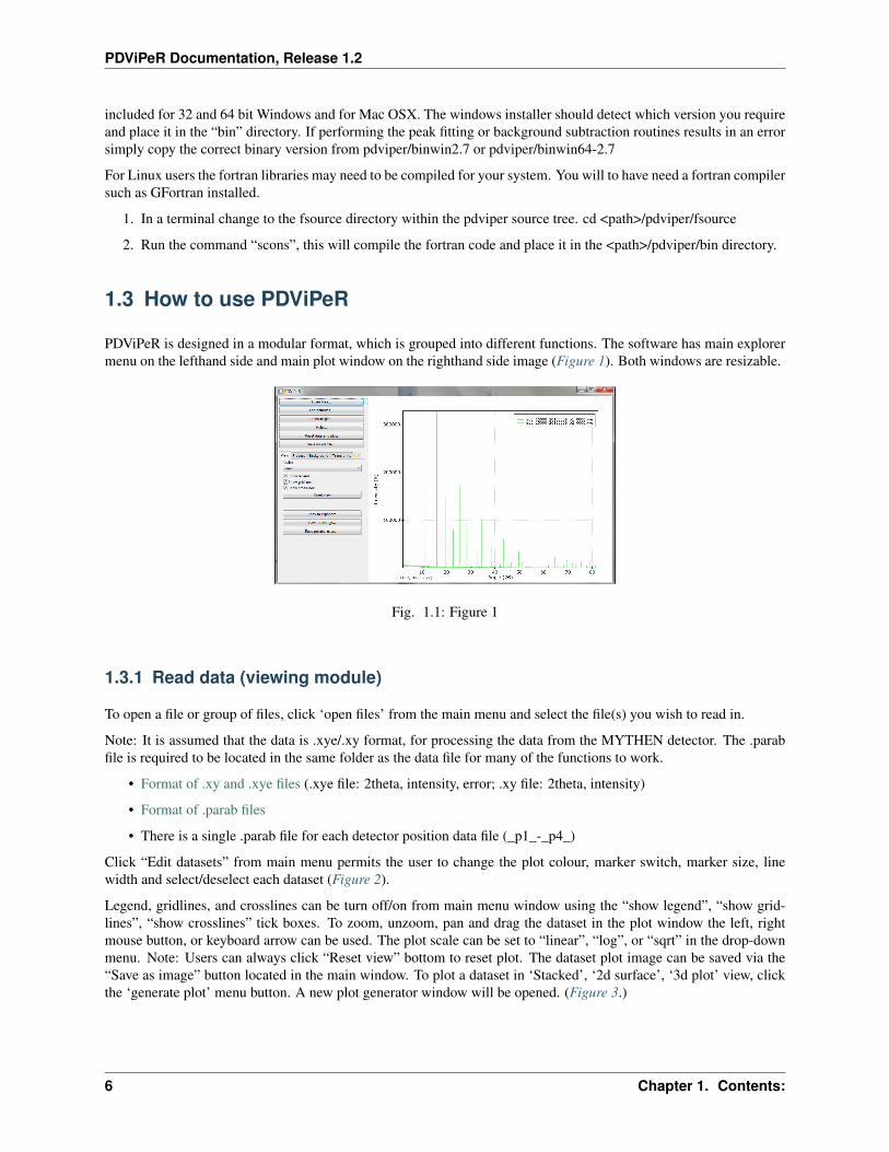
PDViPeR is designed in a modular format, which is grouped into different functions. The software has main explorermenu on the lefthand side and main plot window on the righthand side image (Figure 1). Both windows are resizable.

Fig. 1.1: Figure 1

1.3.1 Read data (viewing module)

To open a file or group of files, click ‘open files’ from the main menu and select the file(s) you wish to read in.

Note: It is assumed that the data is .xye/.xy format, for processing the data from the MYTHEN detector. The .parabfile is required to be located in the same folder as the data file for many of the functions to work.

• Format of .xy and .xye files (.xye file: 2theta, intensity, error; .xy file: 2theta, intensity)

• Format of .parab files

• There is a single .parab file for each detector position data file (_p1_-_p4_)

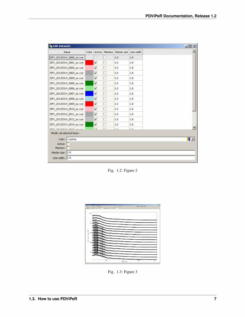
Click “Edit datasets” from main menu permits the user to change the plot colour, marker switch, marker size, linewidth and select/deselect each dataset (Figure 2).

Legend, gridlines, and crosslines can be turn off/on from main menu window using the “show legend”, “show grid-lines”, “show crosslines” tick boxes. To zoom, unzoom, pan and drag the dataset in the plot window the left, rightmouse button, or keyboard arrow can be used. The plot scale can be set to “linear”, “log”, or “sqrt” in the drop-downmenu. Note: Users can always click “Reset view” bottom to reset plot. The dataset plot image can be saved via the“Save as image” button located in the main window. To plot a dataset in ‘Stacked’, ‘2d surface’, ‘3d plot’ view, clickthe ‘generate plot’ menu button. A new plot generator window will be opened. (Figure 3.)

6 Chapter 1. Contents:

PDViPeR Documentation, Release 1.2

Fig. 1.2: Figure 2

Fig. 1.3: Figure 3

1.3. How to use PDViPeR 7

PDViPeR Documentation, Release 1.2

• Stacked plot Adjust the ‘Offset’ and ‘Value range’ slider controls to change space between the data sets andintensity of the dataset. Tick ‘flip order’ to reverse the orderChange the plot scale by selecting ‘linear’, ‘log’,‘sqrt’ options.

• 2d surface Double click the plot axis to change the dataset plot range and label. Drag on the scale bar on theright side of the plot to change plot colour scale. (Figure 4)

Fig. 1.4: Figure 4

• 3d plot Adjust ‘Azimuth’ and/or ‘Elevation’ to change the plot view direction, or drag the plot with left-buttonof mouse (Figure 5). Change the plot label and range in the upper menu. Quality value should be set as ‘1’,when the plot view is changed; Quality value should be set as ‘5’, when plot is output for best resolution.

Fig. 1.5: Figure 5

8 Chapter 1. Contents:

PDViPeR Documentation, Release 1.2

1.3.2 Process module

Merging datasets

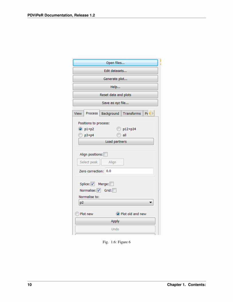
The MYTHEN detector array on the PD beamline covers a total angular range of approximately 80° and consists ofsixteen adjacent microstrip detectors separated by small gaps. Consequently, the acquired array of angle vs intensitydata pairs contain gaps. Two data sets are collected with the detector array offset by a small angle (typically 0.5degrees) to capture data in the gap regions. Motor encoder errors may lead to a systematic uncertainty in the offsetangle (typically ca. 0.001°). The data from an individual capture run from the detector therefore contains gaps andsome systematic uncertainty in both the angle and intensity values. PDViPeR can merge the two datasets to produce asingle contiguous dataset by normalising and offsetting the data. The software also discards poor quality data pointsnear the gap edges. There are two distinct processes used to combine multiple detector position data sets. The first,called merging, simply combines the multiple data sets and sorts on angle thereby generating a contiguous data set.Since most of the data are used from each detector position, the resulting file is considerably larger than the individualdata sets. The second combination method is known as splicing and substitutes the missing data from one data set tothe other to form the contiguous data set. Finally, PDViPeR can concatenate data from two overlapping 80° rangesto produce a dataset with extended range, for example, 0° – 150°. Figure 6 shows the ‘Process’ module tab and theoptions available. The functions and how to use them are described further below:

• Datasets are merged in pairs. Select ‘Positions to process’ according to your dataset, then click ‘Load partners’to load all detector positions. E.g. P1 and P2.

• If users wish to correct any misalignments between detector positions (e.g. P1, P2) via an automated peak fittingalgorithm, tick ‘Align positions’, and click ‘Select peak’. Select a single non-overlapping peak from the mainplot window (this peak must exist for all the datasets to be aligned) and click ‘Align’. This function only workswith ‘P12’ or ‘P34’ options.

• ‘Zero correction’ is used to manually correct known detector 2theta angle error. Default = 0.

• Click ‘Apply’, and ‘Save’ the processed dataset into your desired folder.

• Click ‘Undo’ to reverse the processing.

• The ‘P12+P34’ option is used to merge previously processed P12 and P34 data files. This option stitches twoprocessed datasets together to form an extended angle diffraction pattern (e.g. 0 – 150° 2-Theta) .

• The ‘all’ option is used to merge all unprocessed detector positions at once. (e.g. P1,P2,P3,P4)

Normalising data

If the storage ring is in decay mode, the incoming X-ray beam intensity incident on the sample changes with time.Data sets can be normalised with respect to intensity to remove this effect. It is necessary that one of the available datasets must be the reference from which all other datasets are normalised to. Any particular dataset can be used as thenormalisation reference by selecting the appropriate dataset in the ‘Normalise to:’ field. The default is to normalise toeach dataset’s P1 position.

Regridding data

This is used to generate equally step sized data points. Ticking the ‘Grid’ option regrids the data in 0.00375° stepsusing a linear interpolation.

Note regarding output of grid data:

In order to output data of constant step size it is necessary to interpolate between data point of one or more datafiles. This causes neighbouring data points in the subsequent output to be correlated (because neighbouring points

1.3. How to use PDViPeR 9

PDViPeR Documentation, Release 1.2

Fig. 1.6: Figure 6

10 Chapter 1. Contents:

PDViPeR Documentation, Release 1.2

in the output probably arose from interpolating between 2 points in the input, at least one of which is common toboth of the output points). This correlation destroys the assumption in least squares refinement that the observationsare independent, so strictly speaking it is no longer justifiable to quote the numbers coming out of your refinement(particularly esds). It is therefore preferable to conduct a multi-histogram refinement.

Saving results

Saving processed data files uses particular flags or identifiers in the output file name to indicate what processing hastaken place. The ‘Save...’ option writes .xye files named according to the processing steps applied. The conventionfor the processed data name is as follows:

Table 1.1: Processed datafile naming con-ventions

‘label’ ‘meaning’‘m’ ‘merge’‘s’ ‘splice’‘n’ ‘normalized’‘g’ ‘grid’‘p12’ ‘position P1 and P2 processed’

A log file entry for each written processed file is produced and is called logfile.log.

1.3.3 Background module

There are 3 functions in the background module to allow users to remove the data background. (Figure 7)

• User defined background: Users can define their own background by selecting points on the XRD data. Aminimum of 10 data points are required. Click the ‘Define’ button. After all data points are selected using theleft mouse button, press the ‘enter’ key to fit the background. Click ‘Subtract background’ and ‘Save’ to subtractthe background and save the processed data.

• Loaded background file: A previously collected ‘background’ dataset can be subtracted from each real dataset.In the ‘Background’ tab, click ‘Load’ to load the background file. Click ‘Subtract background’ and the softwarewill subtract the background dataset from all the loaded datasets. Click ‘Save’ to save processed data.

• Automatic background fitting: Polynomial functions can be used to fit the background for subsequent subtrac-tion. Select which polynomial function that is to be used to fit the data. Change the number of fit parameters,then click ‘Curve fit’. Inspect the fitting in the data plot window, if it is not adequate then change the parametersor fitting function. Click ‘Subtract background’ to subtract the background. Then click ‘Save’ to save processeddata.

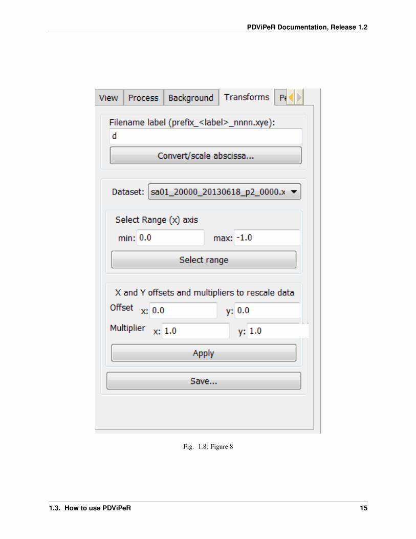
1.3.4 Transforms module

This module is designed for users to convert data between different units ( 2theta, Q and d spacing). Data can also beconverted between different wavelengths to aid comparison of datasets collected at different wavelengths.

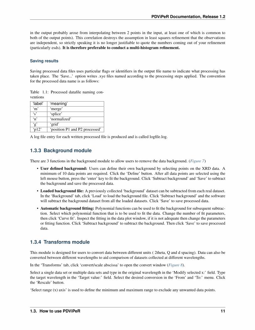
In the ‘Transforms’ tab, click ‘convert/scale abscissa’ to open the convert window (Figure 8).

Select a single data set or multiple data sets and type in the original wavelength in the ‘Modify selected x:’ field. Typethe target wavelength in the ‘Target value:’ field. Select the desired conversion in the ‘From’ and ‘To:’ menu. Clickthe ‘Rescale’ button.

‘Select range (x) axis’ is used to define the minimum and maximum range to exclude any unwanted data points.

1.3. How to use PDViPeR 11

PDViPeR Documentation, Release 1.2

Fig. 1.7: Figure 7

12 Chapter 1. Contents:

PDViPeR Documentation, Release 1.2

The ‘X and Y offsets and multipliers to rescale data’ options are used to rescale data. Click ‘Apply’ and ‘save’ to savemodified data.

1.3. How to use PDViPeR 13

PDViPeR Documentation, Release 1.2

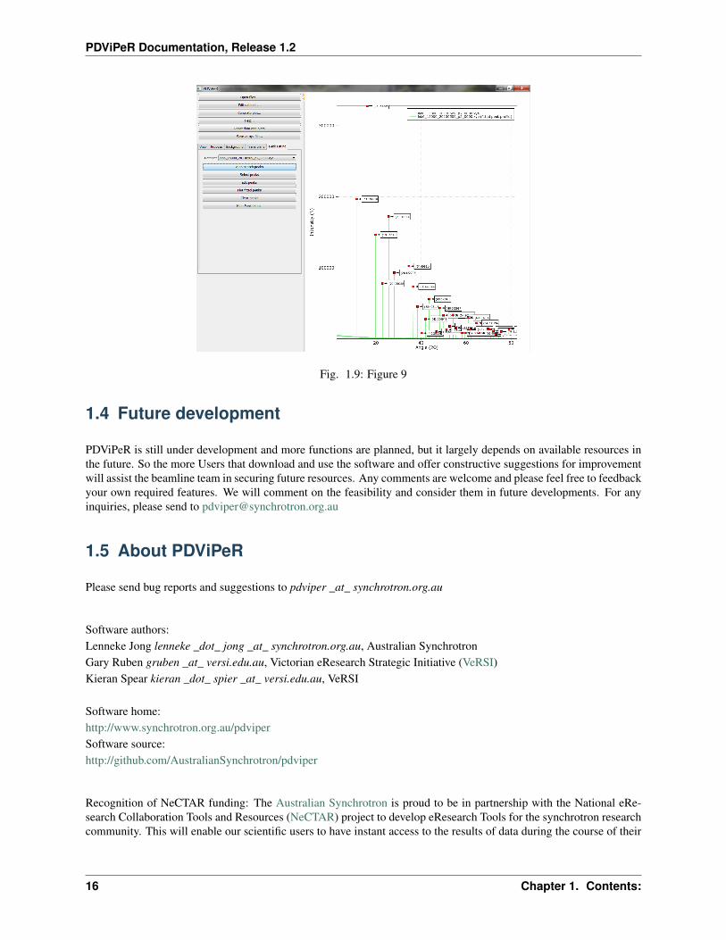
1.3.5 Peak fitting module

The peak fitting module allows users to manually or automatically select the location of peaks and to refine peakprofiles. The selected peaks profile data can subsequently be exported to an indexing program or be used for strain andparticle size analysis. Click the ‘Peak fitting’ tab from the explorer menu to show the peak fitting module. The useris presented with some basic peak analysis tasks, including, automatic and manual peak selection options, and peakfitting and refine options (Figure 9).

• Automatic peak search is performed by clicking the ‘Auto search peaks’ button. The ‘Edit peaks’ window willpop up to allow users to refine or just save the peak list into a .txt file. The peak position, intensity, and FWHMcan be refined.

• Manual peak selection is performed by clicking the ‘Select peaks’ button. To select individual peaks click neareach peak in the data plot window. Once all desired peaks are selected, just press ‘enter’ to finish.

Peak labels can be turned on and off by clicking the “hide peak labels” button. The fitted peak can be turn on and offby clicking the “plot fitted peak” button.

14 Chapter 1. Contents:

PDViPeR Documentation, Release 1.2

Fig. 1.8: Figure 8

1.3. How to use PDViPeR 15

PDViPeR Documentation, Release 1.2

Fig. 1.9: Figure 9

1.4 Future development

PDViPeR is still under development and more functions are planned, but it largely depends on available resources inthe future. So the more Users that download and use the software and offer constructive suggestions for improvementwill assist the beamline team in securing future resources. Any comments are welcome and please feel free to feedbackyour own required features. We will comment on the feasibility and consider them in future developments. For anyinquiries, please send to pdviper@synchrotron.org.au

1.5 About PDViPeR

Please send bug reports and suggestions to pdviper _at_ synchrotron.org.au

Software authors:Lenneke Jong lenneke _dot_ jong _at_ synchrotron.org.au, Australian SynchrotronGary Ruben gruben _at_ versi.edu.au, Victorian eResearch Strategic Initiative (VeRSI)Kieran Spear kieran _dot_ spier _at_ versi.edu.au, VeRSI

Software home:http://www.synchrotron.org.au/pdviperSoftware source:http://github.com/AustralianSynchrotron/pdviper

Recognition of NeCTAR funding: The Australian Synchrotron is proud to be in partnership with the National eRe-search Collaboration Tools and Resources (NeCTAR) project to develop eResearch Tools for the synchrotron researchcommunity. This will enable our scientific users to have instant access to the results of data during the course of their

16 Chapter 1. Contents:

PDViPeR Documentation, Release 1.2

experiment which will facilitate better decision making and also provide the opportunity for ongoing data analysis viaremote access.

1.6 .parab and .xy/.xye file formats

These are documented on the AS PD beamline website.

1.6. .parab and .xy/.xye file formats 17

PDViPeR Documentation, Release 1.2

18 Chapter 1. Contents:

CHAPTER 2

Modules

This section contains auto-generated documentation extracted from the processing module that contains the interpola-tion, alignment and merging algorithms.

2.1 processing

19

PDViPeR Documentation, Release 1.2

20 Chapter 2. Modules

CHAPTER 3

Indices and tables

• genindex

• modindex

• search

21