Embed Size (px)
Citation preview

Table of ContentsTopics:
1) Hydrologic Cycle and Hydrologic Budget
2) R i f ll Hi t i l St2) Rainfall: Historical Storms Design Storms
3) Abstractions: Rainfall Excess
4) Runoff Methods:
Small Catchments: Rational Method
Midsize Catchments: SCS TR55 MethodUnit Hydrograph Method
A diAppendices: A: Hydrologic Design Components for SCSTR 55 B: Hydrologic RoutingC: Groundwater: Well Hydraulics
2
C: Groundwater: Well HydraulicsD: Unit Hydrograph and Additional examples

Hydrologic Cycle and Terms
• Precipitation/Rainfall.
Discharge of water from the atmosphere.
• Rainfall excessRainfall excess.
Rainfall minus interceptiondepression storage
tievaporationinfiltration
• Runoff.Rainfall that appears in surface streamsRainfall that appears in surface streams
(includes subsurface quick return flow).
S f ff
3
• Surface runoff.Runoff which travels over the soil surface to the nearest stream.
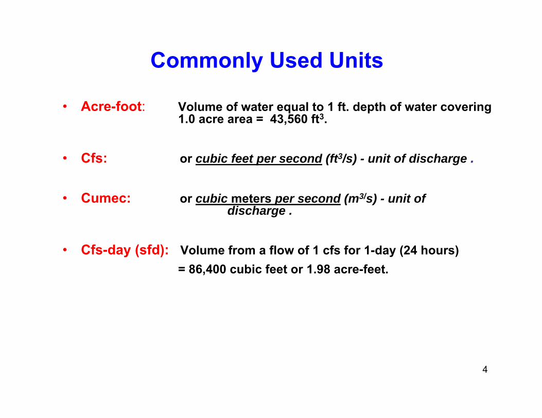
Commonly Used Units
• Acre-foot: Volume of water equal to 1 ft. depth of water covering 1.0 acre area = 43,560 ft3.
• Cfs: or cubic feet per second (ft3/s) - unit of discharge .
• Cumec: or cubic meters per second (m3/s) - unit of discharge .
• Cfs-day (sfd): Volume from a flow of 1 cfs for 1-day (24 hours) = 86,400 cubic feet or 1.98 acre-feet.
4
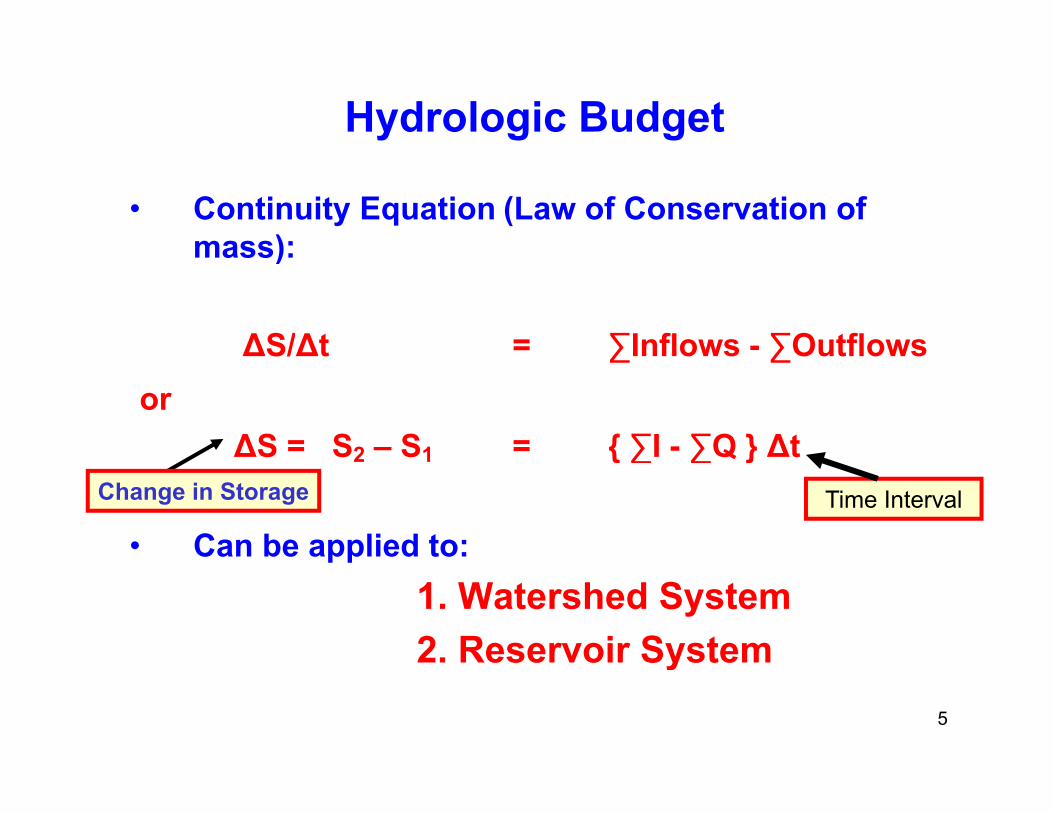
Hydrologic Budget
• Continuity Equation (Law of Conservation of mass):mass):
ΔS/Δt = ∑Inflows - ∑OutflowsΔS/Δt ∑Inflows ∑Outflowsor
ΔS = S2 – S1 = { ∑I - ∑Q } Δt2 1 { ∑ ∑Q }
• Can be applied to:
Change in Storage Time Interval
pp1. Watershed System2. Reservoir System
5
y
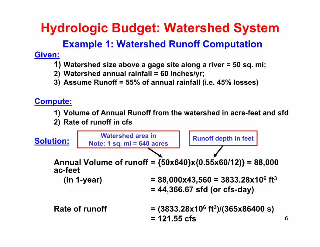
Hydrologic Budget: Watershed SystemExample 1: Watershed Runoff ComputationExample 1: Watershed Runoff Computation
Given:1) Watershed size above a gage site along a river = 50 sq. mi; 2) Watershed annual rainfall = 60 inches/yr; ) y ;3) Assume Runoff = 55% of annual rainfall (i.e. 45% losses)
Compute:1) Volume of Annual Runoff from the watershed in acre-feet and sfd2) Rate of runoff in cfs
S l tiWatershed area in Runoff depth in feetSolution:
Annual Volume of runoff = {50x640}x{0.55x60/12)} = 88,000 ac-feet
Note: 1 sq. mi = 640 acresRunoff depth in feet
ac-feet(in 1-year) = 88,000x43,560 = 3833.28x106 ft3
= 44,366.67 sfd (or cfs-day)
6Rate of runoff = (3833.28x106 ft3)/(365x86400 s)
= 121.55 cfs

Hydrologic Budget: Reservoir SystemExample 2: Reservoir Storage Computation
Given: During a 30 day period:1) Streamflow into the reservoir, Q = 5.0 m3/s2) Water supply withdrawal, W = 136 mgd3) Evaporation from the reservoir surface = 9.40 cm4) Average reservoir water surface = 3.75 km2
5) Beginning reservoir storage S1 = 12 560 ac- ft5) Beginning reservoir storage, S1 = 12,560 ac- ft
Continuity Equation: S2 = S1 + Q – W – E ( ll l it )(all volume units)
Note: Time period ∆t = 30 days = (30x86 400) sec7
Note: Time period ∆t = 30 days = (30x86,400) sec
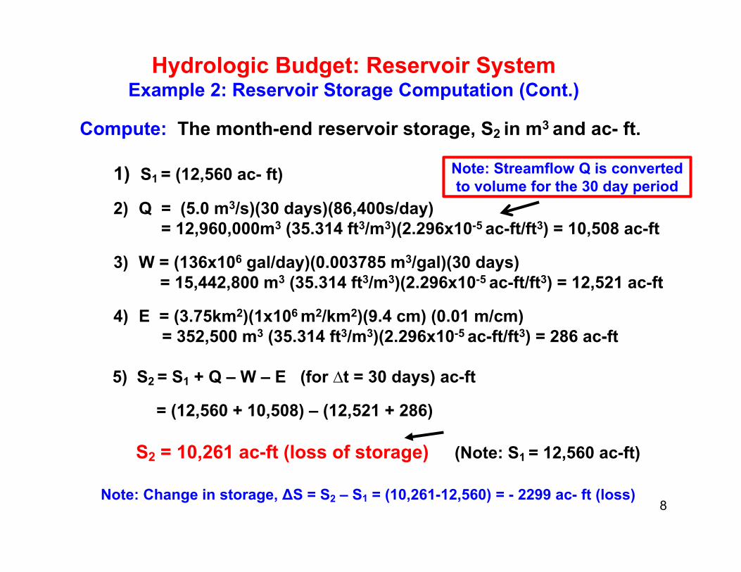
Hydrologic Budget: Reservoir SystemExample 2: Reservoir Storage Computation (Cont.)
Compute: The month-end reservoir storage, S2 in m3 and ac- ft.
1) S1 = (12,560 ac- ft) Note: Streamflow Q is converted 1) S1 (12,560 ac ft)
2) Q = (5.0 m3/s)(30 days)(86,400s/day)= 12,960,000m3 (35.314 ft3/m3)(2.296x10-5 ac-ft/ft3) = 10,508 ac-ft
to volume for the 30 day period
3) W = (136x106 gal/day)(0.003785 m3/gal)(30 days) = 15,442,800 m3 (35.314 ft3/m3)(2.296x10-5 ac-ft/ft3) = 12,521 ac-ft
4) E = (3.75km2)(1x10⁶ m2/km2)(9.4 cm) (0.01 m/cm) ) ( )( )( ) ( )= 352,500 m3 (35.314 ft3/m3)(2.296x10-5 ac-ft/ft3) = 286 ac-ft
5) S2 = S1 + Q – W – E (for ∆t = 30 days) ac-ft
= (12,560 + 10,508) – (12,521 + 286)
S2 = 10,261 ac-ft (loss of storage) (Note: S1 = 12,560 ac-ft)
8Note: Change in storage, ΔS = S2 – S1 = (10,261-12,560) = - 2299 ac- ft (loss)
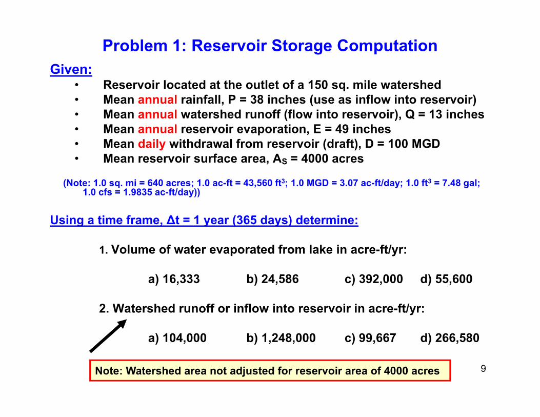
Problem 1: Reservoir Storage ComputationGiven:
• Reservoir located at the outlet of a 150 sq. mile watershed• Mean annual rainfall, P = 38 inches (use as inflow into reservoir)• Mean annual watershed runoff (flow into reservoir), Q = 13 inches• Mean annual reservoir evaporation E = 49 inches• Mean annual reservoir evaporation, E = 49 inches• Mean daily withdrawal from reservoir (draft), D = 100 MGD• Mean reservoir surface area, AS = 4000 acres
(Note: 1 0 sq mi = 640 acres; 1 0 ac ft = 43 560 ft3; 1 0 MGD = 3 07 ac ft/day; 1 0 ft3 = 7 48 gal;(Note: 1.0 sq. mi = 640 acres; 1.0 ac-ft = 43,560 ft3; 1.0 MGD = 3.07 ac-ft/day; 1.0 ft3 = 7.48 gal; 1.0 cfs = 1.9835 ac-ft/day))
Using a time frame, Δt = 1 year (365 days) determine:
1. Volume of water evaporated from lake in acre-ft/yr:
a) 16,333 b) 24,586 c) 392,000 d) 55,600
2. Watershed runoff or inflow into reservoir in acre-ft/yr:
a) 104 000 b) 1 248 000 c) 99 667 d) 266 580
9
a) 104,000 b) 1,248,000 c) 99,667 d) 266,580
Note: Watershed area not adjusted for reservoir area of 4000 acres

Problem 1: Reservoir Storage Computation (cont.)
3. Watershed runoff or inflow into reservoir in cfs:
a) 250.8 b) 143.7 c) 550.0 d) 85.6
4. Volume of rainfall input, P, to reservoir in acre-ft/yr
a) 152,000 b) 304,000 c) 12,667 d) 85,000
5. Mean draft, D in ac-ft/yr:
a) 100,000 b) 112,055 c) 185,250 d) 265,500
6 N t l / i f i t ΔS i ft/6. Net loss/gain of reservoir storage, ΔS in acre-ft/yr:
a) -16,280 b) 12,500 c) -11,721 d) 0
10
Computation of Critical (Maximum) SReservoir Storage
• Graphical Method:Mass Curve Analysis (Rippl Method)Mass Curve Analysis (Rippl Method)
A l ti l M th d• Analytical Method:Sequent Peak Method
11
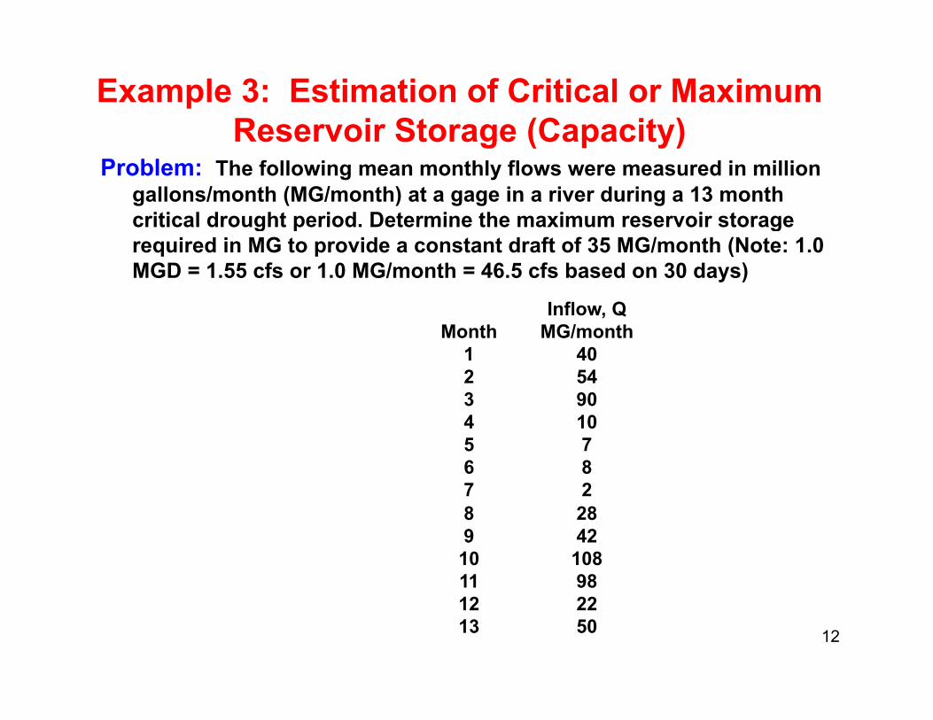
Example 3: Estimation of Critical or Maximum Reservoir Storage (Capacity)Reservoir Storage (Capacity)
Problem: The following mean monthly flows were measured in million gallons/month (MG/month) at a gage in a river during a 13 month critical drought period Determine the maximum reservoir storagecritical drought period. Determine the maximum reservoir storage required in MG to provide a constant draft of 35 MG/month (Note: 1.0 MGD = 1.55 cfs or 1.0 MG/month = 46.5 cfs based on 30 days)
Inflow, QInflow, QMonth MG/month
1 402 543 903 904 105 76 87 28 289 4210 10811 98
12
11 9812 2213 50

Example 3: Mass Curve Analysis for Estimating Critical Reservoir Capacity Rippl Method (cont )
600
Critical Reservoir Capacity- Rippl Method (cont.)
Tangent to Cum. Draft Line
400
500
n
Required Critical Reservoir Storage (Capacity)=(350-230) = 120 MG
P2
300
m. Q
or D
inG
/ M
onth
(350 230) 120 MG
P1
100
200
Cum M
G
Cumulative Inflow
Cumulative
P1 T1
01 2 3 4 5 6 7 8 9 10 11 12 13
Month
Draft
13
Month

Example 3: Analytical Solution (Sequent Peak Method) (cont.)
Inflow, Q Draft, D Cum. Q Cum. D Cum Q - Cum DMonth MG/month MG/month MG/month MG/month MG/month
1 40 35 40 35 5
) ( )
2 54 35 94 70 243 90 35 184 105 79 P14 10 35 194 140 545 7 35 201 175 266 8 35 209 210 -17 2 35 211 245 -348 28 35 239 280 -41 T19 42 35 281 315 -3410 108 35 389 350 3911 98 35 487 385 102 P212 22 35 509 420 89 T213 50 35 559 455 104 P3
Required Reservoir Storage = Max{ (P1-T1) or (P2 - T2) } = (79-(-41)) or (102 - 89)
14
= 120 MG

RAINFALLT t f i f ll tTwo types of rainfall events:
1) HISTORICAL:
– Spatially and temporally averaged hyetographs rainfall events– Based on measured rainfall depths using rain gages at a point
HyetographHyetograph
0 5
0.8
1.8
0.751
1.251.5
1.752
Rain
fall
((cm
)
A 12- hour historical rainfall event Incremental depths:Time (h): 0-3 3-6 6-9 9-12 Rainfall (cm): 0.50 0.80 1.80 0.40Intensity (cm/hr): 0 17 0 27 0 60 0 130.5 0.4
00.25
0.5
0 - 3 3 - 6 6 - 9 9 - 12
Time (h)
Ra Intensity (cm/hr): 0.17 0.27 0.60 0.13
2) DESIGN (or SYNTHETIC):
– Standardized temporal rainfall distributions (design storm hyetographs)
15
p ( g y g p )– Based on regionalized historical rainfall data for select duration and
frequency

Design Rainfall Intensity-Duration-Frequency (IDF)Intensity Duration Frequency (IDF)
Requires the following:
1) Frequency (F ) or average return period (T) (see Appendix A)1) Frequency (FR) or average return period (T) (see Appendix A)
Example: For T = 100 years, FR = 1/T = 1/100 = 0.01 or 1%
2) Duration td Usually assumed equal to time of concentration t c2) Duration, td
3) Design rainfall depth = (intensity x duration)
Obt i d f Based on T and td
Usually assumed equal to time of concentration, t c
Obtained from:
a) NWS TP 40 Regionalized Rainfallb) From Intensity Duration Frequency (IDF) Curves or Equations
Based on T and td
b) From Intensity Duration Frequency (IDF) Curves or Equations
4) Time (or temporal) distribution of rainfall depth
5) Spatial variation rainfall depth over a catchment
Rainfall Hyetograph
16Handled using an average rainfall depth
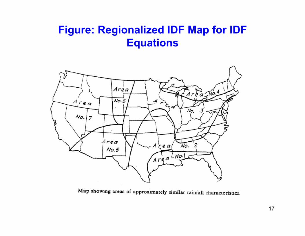
Figure: Regionalized IDF Map for IDF EquationsEquations
17

Table: Regionalized IDF Equations
18
a) From the IDF Curves for Louisville Kentucky:
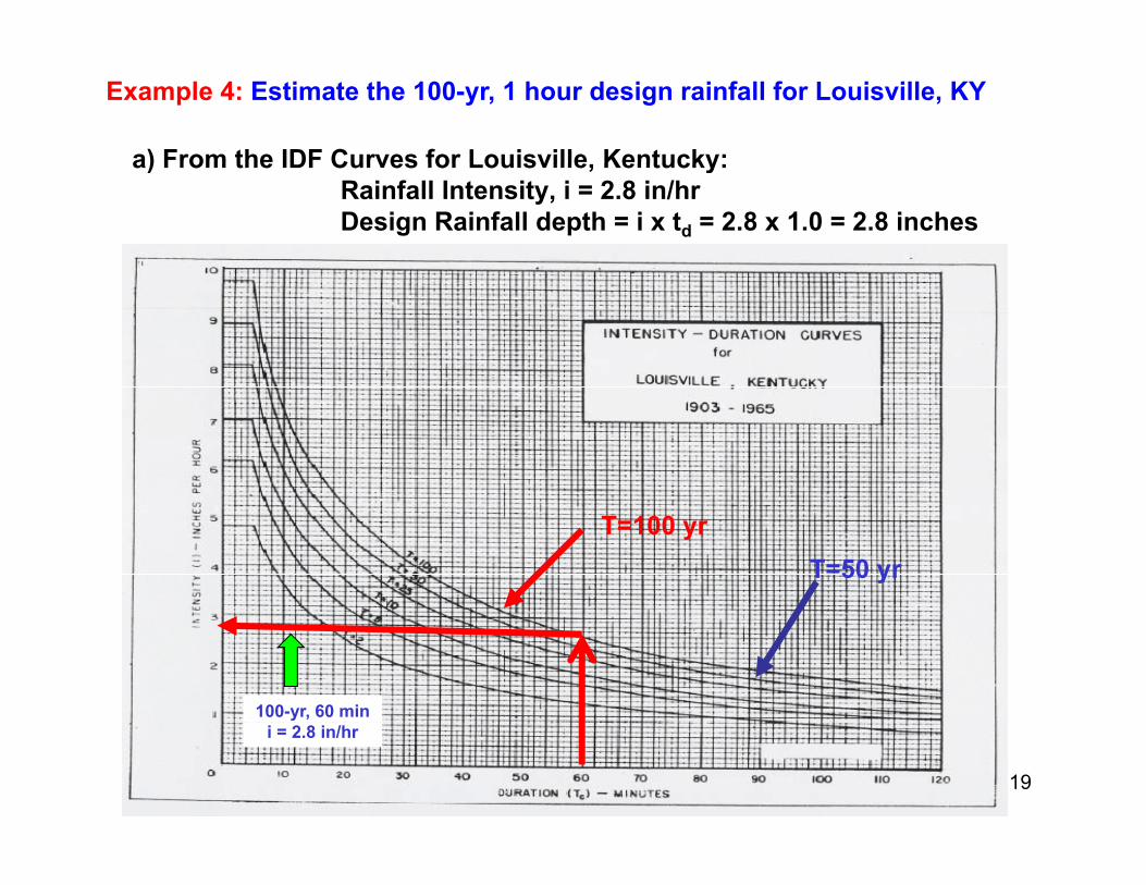
Example 4: Estimate the 100-yr, 1 hour design rainfall for Louisville, KY
a) From the IDF Curves for Louisville, Kentucky:Rainfall Intensity, i = 2.8 in/hr Design Rainfall depth = i x td = 2.8 x 1.0 = 2.8 inches
T=100 yrT=50 yr
100-yr, 60 min
19
i = 2.8 in/hr

Example 4: Estimate the 100-yr, 1 hour design rainfall for Louisville, KY (cont.)
b) From the IDF Map and Table (Slides 17 and 18) Louisville is in Region 3Region 3. Regional IDF equation for T =100 yr :i (mm/hr) = { 7370/(t+31) } where t = td in minutes
i = 7370/(60+31) = 80.989 mm/hr = 3.2 in/hr
Rainfall Depth = 3.2 in From Louisville IDF Curve P = 2.80 in (see previous slide)
• Note the difference between using a locally developed IDF curve versus using a regional equation
20
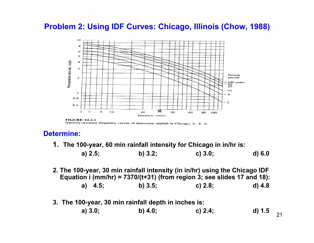
Problem 2: Using IDF Curves: Chicago, Illinois (Chow, 1988)
Determine:
30
1. The 100-year, 60 min rainfall intensity for Chicago in in/hr is:a) 2.5; b) 3.2; c) 3.0; d) 6.0
2. The 100-year, 30 min rainfall intensity (in in/hr) using the Chicago IDF Equation i (mm/hr) = 7370/(t+31) (from region 3; see slides 17 and 18):
a) 4.5; b) 3.5; c) 2.8; d) 4.8
21
3. The 100-year, 30 min rainfall depth in inches is:a) 3.0; b) 4.0; c) 2.4; d) 1.5

AbstractionsAbstractions
Effective Rainfall (or rainfall excess), Pe equals( ), e q
Rainfall (P) minus
Abstractions due to: fInfiltration
Depression Storage InterceptionInterception
22Rainfall Excess = Volume of Direct Runoff, Q
Abstractions (Cont.)( )
• Main Abstraction Process is Infiltration
• Interception and Depression Storage foccur in the early stages of event and can
be considered as initial losses
• Some methods for infiltration: • Infiltration Indices: Φ index• Runoff Coefficients: Rational Method – C• SCS Curve Number Method, CN• Infiltration Capacity Curves: Horton's
23
Infiltration Capacity Curves: Horton s
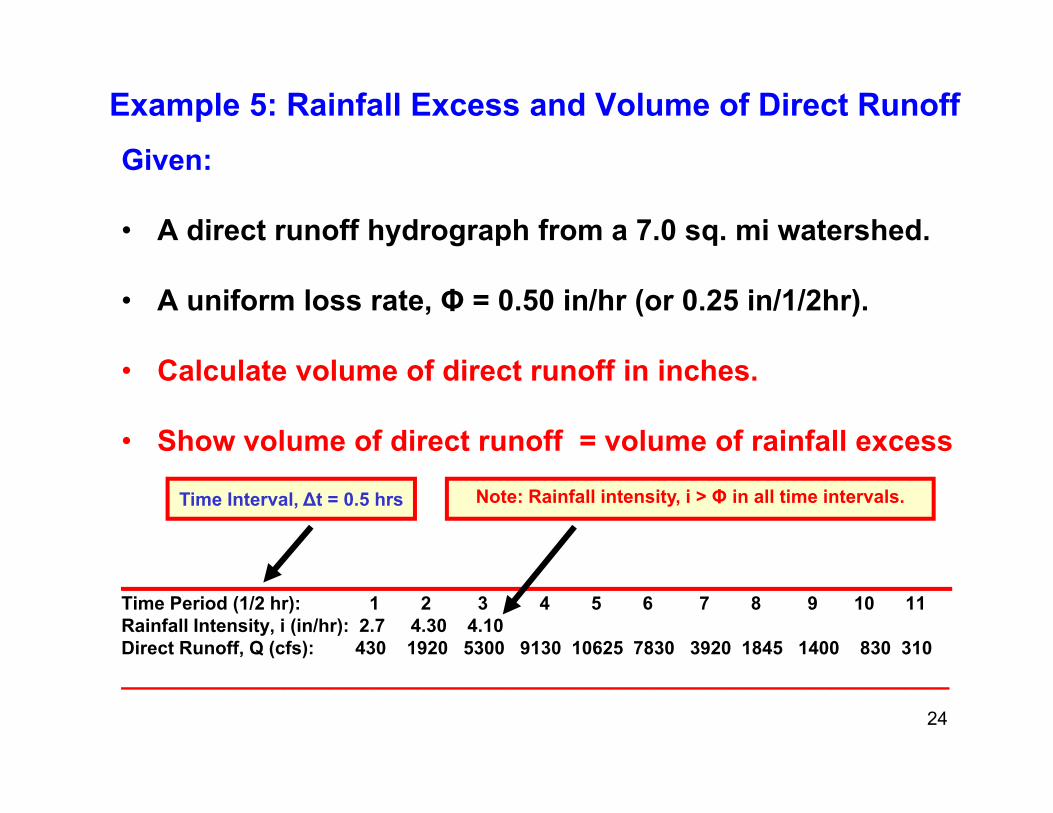
Example 5: Rainfall Excess and Volume of Direct RunoffGiGiven:
• A direct runoff hydrograph from a 7.0 sq. mi watershed.
• A uniform loss rate, Φ = 0.50 in/hr (or 0.25 in/1/2hr).
• Calculate volume of direct runoff in inches.
• Show volume of direct runoff = volume of rainfall excess
Time Interval, Δt = 0.5 hrs Note: Rainfall intensity, i > Φ in all time intervals.
________________________________________Time Period (1/2 hr): 1 2 3 4 5 6 7 8 9 10 11Rainfall Intensity, i (in/hr): 2.7 4.30 4.10Direct Runoff, Q (cfs): 430 1920 5300 9130 10625 7830 3920 1845 1400 830 310
24
________________________________________________________
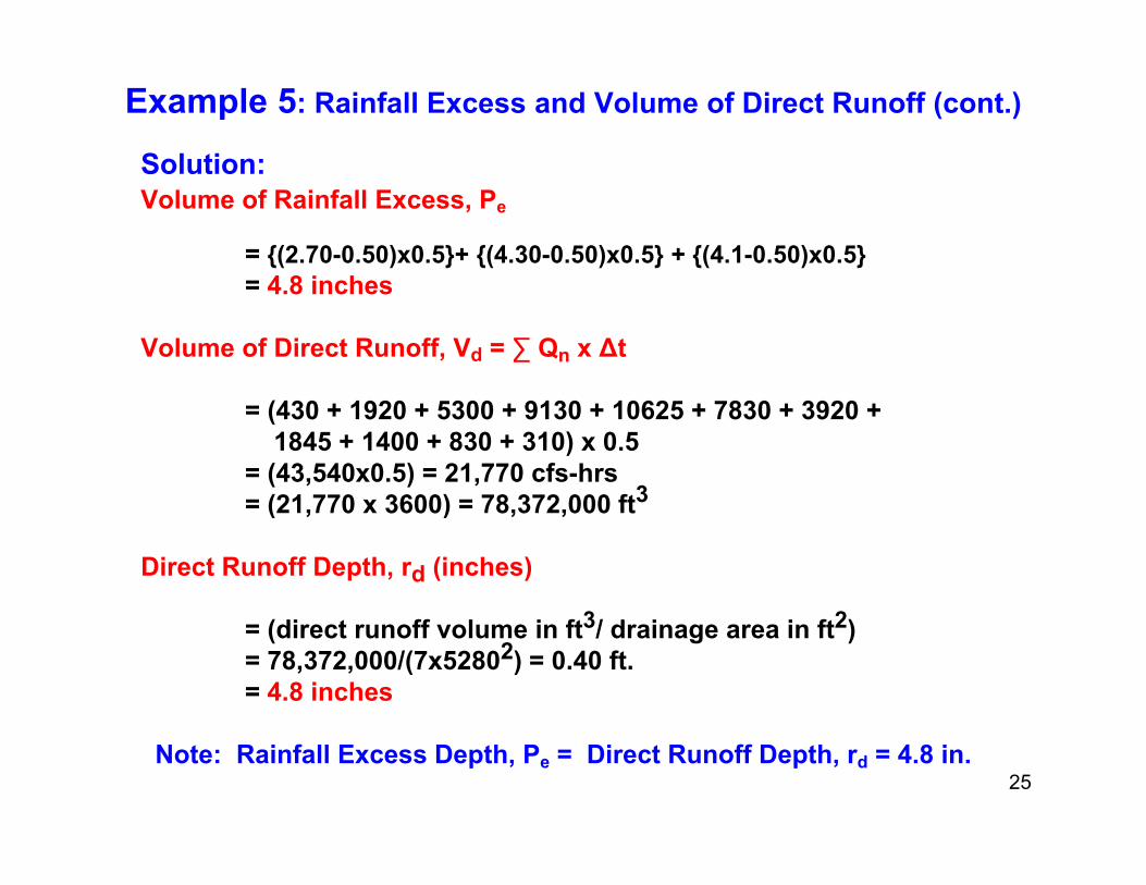
Example 5: Rainfall Excess and Volume of Direct Runoff (cont.)
Solution:Solution:Volume of Rainfall Excess, Pe
= {(2.70-0.50)x0.5}+ {(4.30-0.50)x0.5} + {(4.1-0.50)x0.5}= 4.8 inches
Volume of Direct Runoff, Vd = ∑ Qn x Δt
= (430 + 1920 + 5300 + 9130 + 10625 + 7830 + 3920 + 1845 + 1400 + 830 + 310) x 0.5
= (43,540x0.5) = 21,770 cfs-hrs (21 770 3600) 78 372 000 ft3= (21,770 x 3600) = 78,372,000 ft3
Direct Runoff Depth, rd (inches)
= (direct runoff volume in ft3/ drainage area in ft2) = 78,372,000/(7x52802) = 0.40 ft. = 4.8 inches
25Note: Rainfall Excess Depth, Pe = Direct Runoff Depth, rd = 4.8 in.
Runoff Methods
1. Peak Discharge, Qp, Methods:1. Peak Discharge, Qp, Methods:
• Rational Method
• SCS Curve Number Method(and TR 55 Graphical Peak Discharge Method)
2. Unit Hydrograph Method26
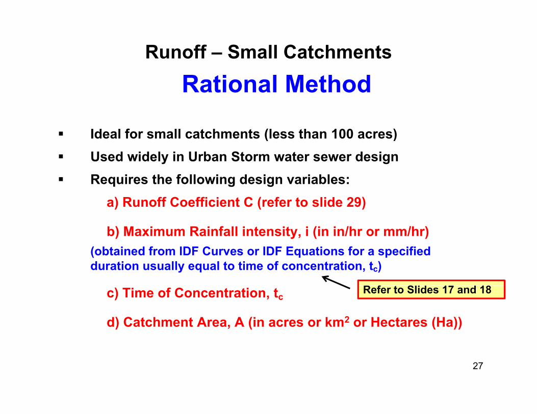
Runoff – Small Catchments
R ti l M th dRational Method
Id l f ll h (l h 100 )Ideal for small catchments (less than 100 acres)Used widely in Urban Storm water sewer designRequires the following design variables:Requires the following design variables:
a) Runoff Coefficient C (refer to slide 29)
b) Maximum Rainfall intensity i (in in/hr or mm/hr)b) Maximum Rainfall intensity, i (in in/hr or mm/hr)(obtained from IDF Curves or IDF Equations for a specified duration usually equal to time of concentration, tc)
f Sc) Time of Concentration, tc
d) Catchment Area, A (in acres or km2 or Hectares (Ha))
Refer to Slides 17 and 18
27
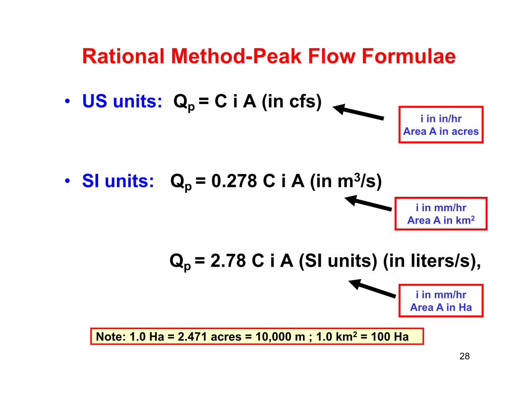
Rational Method-Peak Flow Formulae
• US units: Qp = C i A (in cfs) i in in/hr
SI it Q 0 278 C i A (i 3/ )
Area A in acres
• SI units: Qp = 0.278 C i A (in m3/s) i in mm/hr
Area A in km2
Qp = 2.78 C i A (SI units) (in liters/s), i in mm/hr
Area A in Ha
28
Note: 1.0 Ha = 2.471 acres = 10,000 m ; 1.0 km2 = 100 Ha

Table: Runoff Coefficients, CFor the Rational Method:
29

Time of Concentration, tc
Definition:
tC = ∑travel times from the hydraulically remotest point in a catchmentcatchment
= (Overland flow time) + (Channel or Pipe flow) time
Refer to Appendix A for Methods for Computing Time of Concentration
t3t4
Example: tc at this outlet
30
p= max (t1 + t2) or t3 or t4
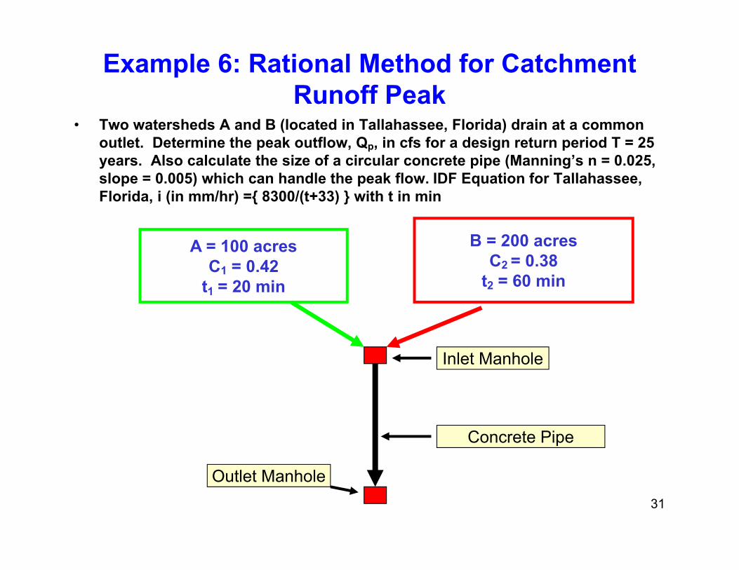
Example 6: Rational Method for Catchment Runoff Peak
• Two watersheds A and B (located in Tallahassee, Florida) drain at a common outlet. Determine the peak outflow, Qp, in cfs for a design return period T = 25 years. Also calculate the size of a circular concrete pipe (Manning’s n = 0.025, slope = 0 005) which can handle the peak flow IDF Equation for Tallahasseeslope = 0.005) which can handle the peak flow. IDF Equation for Tallahassee, Florida, i (in mm/hr) ={ 8300/(t+33) } with t in min
A = 100 acres B = 200 acresA 100 acresC1 = 0.42
t1 = 20 minC2 = 0.38
t2 = 60 min
Inlet Manhole
Concrete Pipe
31
Outlet Manhole

Example 6: Rational Method for Catchment Runoff Peak (cont.)
• Composite Cc = (C1A1 + C2A2)/(A1+A2) • = (0.42x100 + 0.38x200)/(100+200) = 0.39
Note for multiple areas: Q C (∑C /∑ ) ∑C
• Time of Concentration, tc = max ( t1, t2) = max (20, 60) = 60 min
Qp = Cc i AT = (∑Ci i /∑Ai) AT = i ∑CiAiwhere total area, A T = ∑A i
( ) ( )
• 25-year Rainfall intensity I for tc = 60 min = 3.5 in/hr
Tallahassee, FL, IDF Eq. Area 1 (slide 18)i (mm/hr) ={8300/(t+33)} with t in min
• Peak Flow Qp = CciA = 0.39x3.5x300 = 409.5 cfsFrom Manning’s (US Units)
Rational Method Formula (US units)
• Pipe diameter, D = { 2.16x409.5x0.020/ (0.005)0.5 }3/8 = 7.93 feet= 95 2 inches (Use 96 inch pipe)
From Manning’s (US Units)D = (2.16xQpn/√So)3/8
32
= 95.2 inches (Use 96 inch pipe)

Problem 3: Application of Rational Method in Storm Sewer Design
Given:IDF Equation for the area is:
i (in/hr) = 120T 0.175
(t + 27)(td + 27)where T = Return Period in years
td = Storm duration = time of concentration, tc (in minutes) , ( )
Pipe EB
Elv. E = 498.43 ft; Elv. B = 495.55Length of pipe EB = 450 ft
33
Determine Peak Flow from Sub-area Area III and Pipe size EB Using Rational Method

Problem 3: Application of Rational Method in Storm Sewer Design (cont.)
Answer the following questions for a rainfall event with a return period T = 5-yrs :
1) The maximum rainfall intensity i in in/hr is: a) 2.5; b) 5.2; c) 4.3; d) 3.5
2) The peak flow Qp (in cfs) using rational method formula) from Area III into inlet E is:
a) 5.5; b) 10.3; c) 15.2; d) 75.5Qp = CiA
3) The slope S0 of pipe EB is:a) 0.005; b) 0.00034; c) 0.0002; d) 0.0064
4) Th i d di t f i EB (i i h ) t4) The required diameter of sewer pipe EB (in inches) to handle peak flow Qp is (assume n =0.015):
a) 15.2; b) 32.6; c) 25.8; d) 20.5
34From Manning’s (US Units)
D = (2.16xQpn/√So)3/8
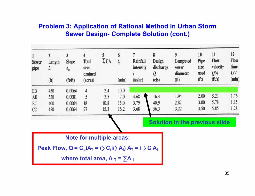
Problem 3: Application of Rational Method in Urban Storm Sewer Design- Complete Solution (cont.) g p ( )
Solution in the previous slide
Note for multiple areas:
Peak Flow, Q = CciAT = (∑Cii/∑Ai) AT = i ∑CiAi
where total area, A T = ∑A i
35
where total area, A T ∑A i
Runoff - Midsize Catchments:
SCS TR55 Method
36

Runoff - Midsize Catchments: SCS TR55 MethodRequires:
C l ti 24 h D i R i f ll d th P (i i h ) f l t d• Cumulative 24-hour Design Rainfall depth, P (in inches) for a selected return period, T (frequency)
37
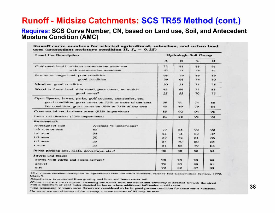
Runoff - Midsize Catchments: SCS TR55 Method (cont.)Requires: SCS Curve Number, CN, based on Land use, Soil, and Antecedent Moisture Condition (AMC)( )
38
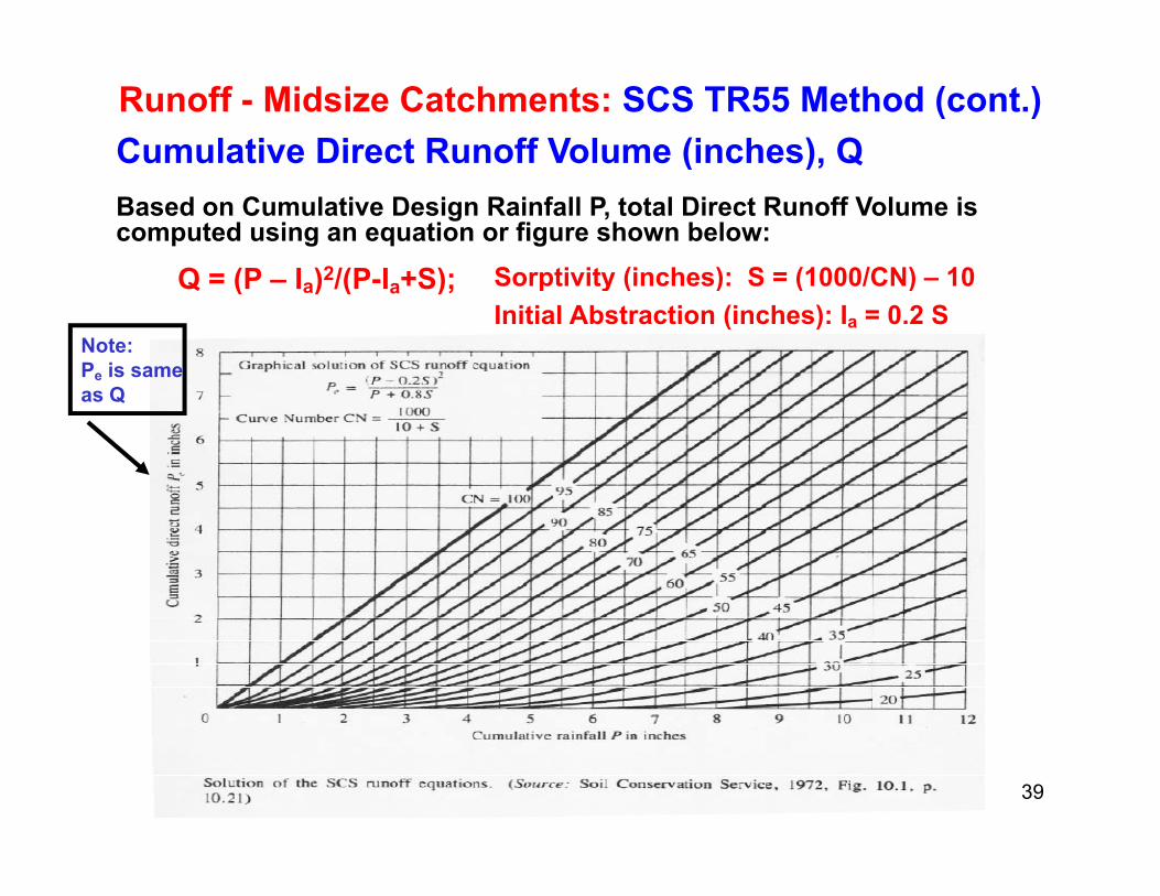
Runoff - Midsize Catchments: SCS TR55 Method (cont.)Cumulative Direct Runoff Volume (inches), Q( ),Based on Cumulative Design Rainfall P, total Direct Runoff Volume is computed using an equation or figure shown below:
Q = (P I )2/(P I +S); Sorptivity (inches): S = (1000/CN) – 10Q = (P – Ia)2/(P-Ia+S); Sorptivity (inches): S = (1000/CN) – 10Initial Abstraction (inches): Ia = 0.2 S
Note: Pe is same as Qas Q
39
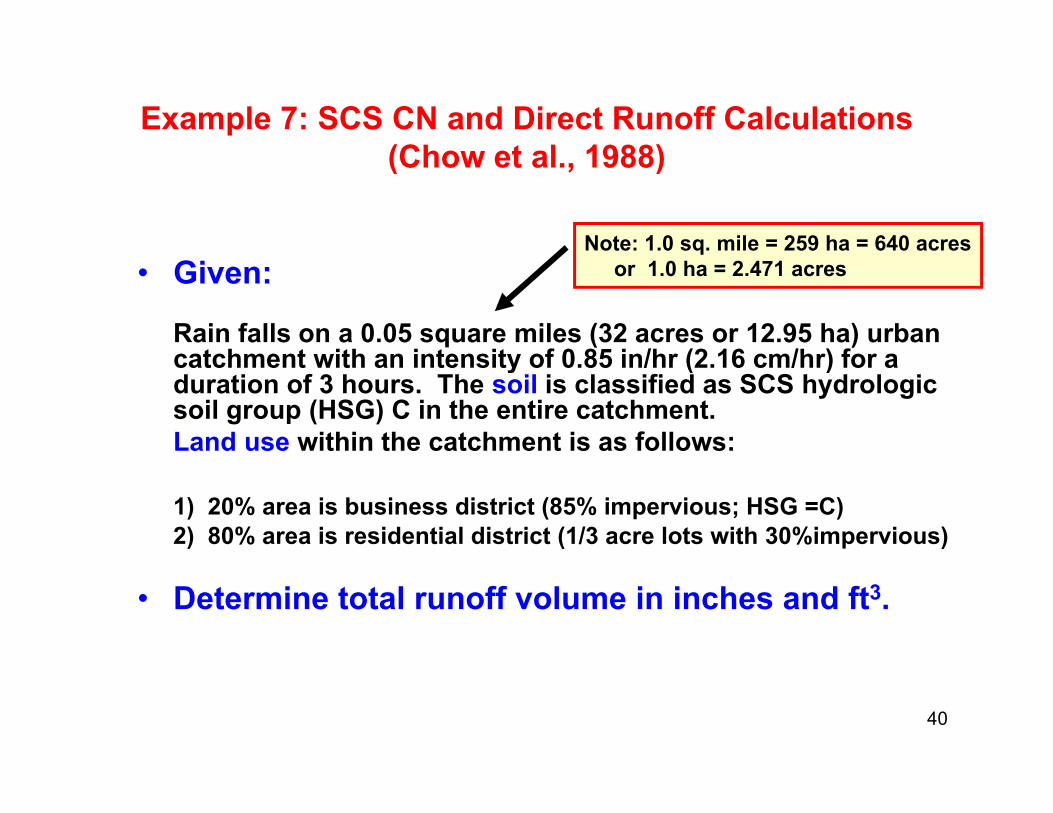
Example 7: SCS CN and Direct Runoff Calculations (Ch t l 1988)(Chow et al., 1988)
Note: 1.0 sq. mile = 259 ha = 640 acres• Given:
Rain falls on a 0.05 square miles (32 acres or 12.95 ha) urban catchment with an intensity of 0 85 in/hr (2 16 cm/hr) for a
qor 1.0 ha = 2.471 acres
catchment with an intensity of 0.85 in/hr (2.16 cm/hr) for a duration of 3 hours. The soil is classified as SCS hydrologic soil group (HSG) C in the entire catchment. Land use within the catchment is as follows:
1) 20% area is business district (85% impervious; HSG =C)2) 80% area is residential district (1/3 acre lots with 30%impervious)
• Determine total runoff volume in inches and ft3.
40

Example 7: SCS CN and Direct Runoff Calculations (cont.) (Chow et al., 1988)
S l tiSolution:
1. Determine SCS Composite CN:
Note: From CN Table for HSG C (Slide 38):Imperious Area CN = 98Open space in good condition CN =74
• Business District CN = ( 0.85x98 + 0.15x74 ) = 94
• Residential District (1/3 acre lots) CN = ( 0.30x98 + 0.70x74 ) = 81
• Composite CN for Catchment CN = ( 0.20x94 + 0.80x81 ) = 83.6
Note: In computing Composite CN in urban areas any area not urbanized is assumed to be open space in good hydrologic condition (see SCS Curve Number, CN Table foot-note 4 – Slide 38).
41
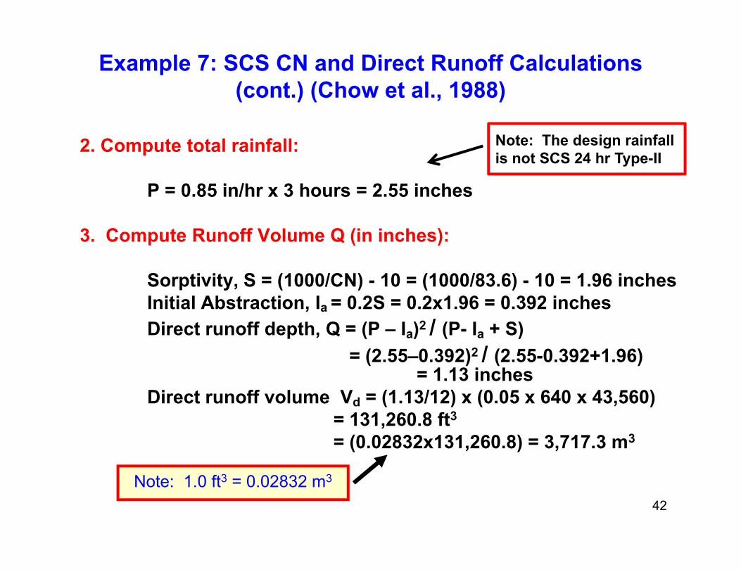
Example 7: SCS CN and Direct Runoff Calculations (cont.) (Chow et al., 1988)
2. Compute total rainfall: Note: The design rainfall is not SCS 24 hr Type-II
P = 0.85 in/hr x 3 hours = 2.55 inches
3. Compute Runoff Volume Q (in inches):
Sorptivity, S = (1000/CN) - 10 = (1000/83.6) - 10 = 1.96 inchesInitial Abstraction, Ia = 0.2S = 0.2x1.96 = 0.392 inchesDi t ff d th Q (P I )2 / (P I S)Direct runoff depth, Q = (P – Ia)2 / (P- Ia + S)
= (2.55–0.392)2 / (2.55-0.392+1.96) = 1.13 inches
Direct runoff volume V = (1 13/12) x (0 05 x 640 x 43 560)Direct runoff volume Vd = (1.13/12) x (0.05 x 640 x 43,560) = 131,260.8 ft3
= (0.02832x131,260.8) = 3,717.3 m3
42
Note: 1.0 ft3 = 0.02832 m3

Problem 4: Calculating SCS CN and Direct Runoff, Q
An undeveloped 1000 acre catchment currently is covered by pasture in good condition and is composed of hydrologic soil
C Thi i d l t it SCS CNgroup C. This gives a pre-development composite SCS CN equal to 74
A proposed urban development (post development) willA proposed urban development (post development) will change the land use to:
1) 55% 1/3 acre lots (30% impervious) CN = 81;1) 55% 1/3 acre lots (30% impervious), CN = 81;
2) 20 % in open space in good condition, CN = 74;
3) 25% in roads, sewers and parking lots, CN = 98.
N t R f t SCS CN T bl Slid 38 f b43
Note: Refer to SCS CN Table, Slide 38 for curve numbers.
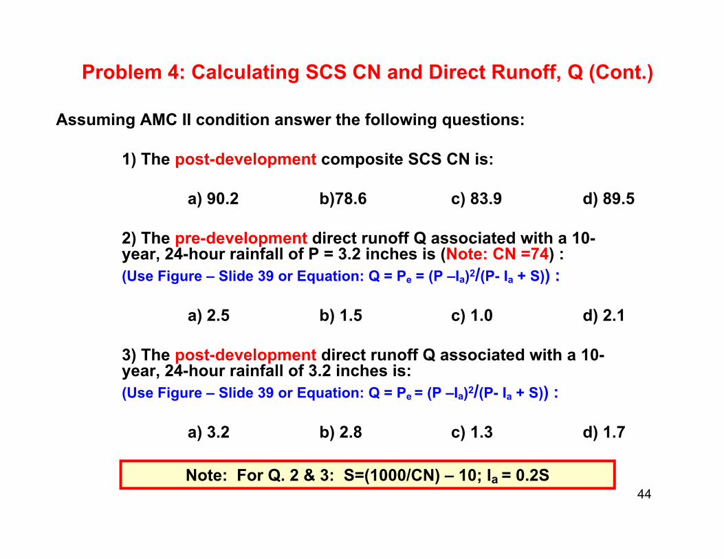
Problem 4: Calculating SCS CN and Direct Runoff, Q (Cont.)
Assuming AMC II condition answer the following questions:
1) The post-development composite SCS CN is:
a) 90.2 b)78.6 c) 83.9 d) 89.5
2) The pre-development direct runoff Q associated with a 10-) p p Qyear, 24-hour rainfall of P = 3.2 inches is (Note: CN =74) : (Use Figure – Slide 39 or Equation: Q = Pe = (P –Ia)2/(P- Ia + S)) :
a) 2 5 b) 1 5 c) 1 0 d) 2 1a) 2.5 b) 1.5 c) 1.0 d) 2.1
3) The post-development direct runoff Q associated with a 10-year, 24-hour rainfall of 3.2 inches is:
/(Use Figure – Slide 39 or Equation: Q = Pe = (P –Ia)2/(P- Ia + S)) :
a) 3.2 b) 2.8 c) 1.3 d) 1.7
44Note: For Q. 2 & 3: S=(1000/CN) – 10; Ia = 0.2S

Runoff - Midsize Catchments: SCS TR55 Method
P k Fl ( f ) Q A Q F
Peak Discharge, Qp computation:
• Peak Flow (cfs): Qp = qu A Q F
where: it k di h ( f / i/i )qu = unit peak discharge (cfs/sq. mi/in)
A = watershed size in sq. milesQ = Volume of direct runoff in inchesF = Pond Factor (depends on % natural storage in ponds
d l k A 1 0 if t li ibl )and lakes. Assume 1.0 if storage negligible)
•Requires:
U it k di h b d G hi l M th d• Unit peak discharge, qu, based on Graphical Method
• Time of Concentration, tc = (∑Overland +
45
, c (∑Channel Flow)

Runoff - Midsize Catchments: SCS TR55 MethodComputing Catchment’s Time of Concentration
SCS TR55 ses the follo ing flo pathsSCS TR55 uses the following flow paths for computing catchment's time of concentration:concentration:
1. Overland Sheet Flow (<300 feet)1. Overland Sheet Flow ( 300 feet)2. Overland Shallow Concentrated Flow3. Channel or Pipe Flow
46

SCS TR55 Method (cont.)1) Equations for Computing Overland Sheet Flow
Time:
US Units: t = 0.007(nL)0.8
P20.5S0.4
SI Units: t = 0.02887(nL)0.8
P20.5S0.4
hwhere:t = travel time in hours; S = average land slope in feet/foot (or meters/meter in SI)n = Manning's overland roughness coefficient (see Slide 48)n Manning s overland roughness coefficient (see Slide 48)L = overland flow distance in feet (or meters for SI units)P2 = 2-Year, 24-hour rainfall depth in inches (or cms for SI units)
47
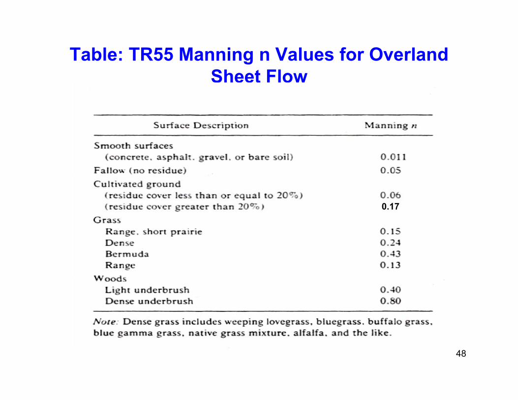
Table: TR55 Manning n Values for Overland Sheet FlowSheet Flow
0.17
48
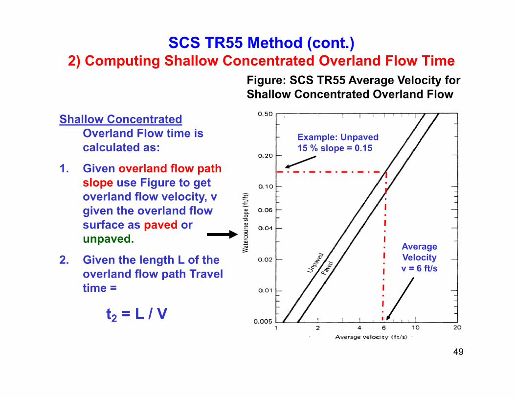
SCS TR55 Method (cont.) 2) Computing Shallow Concentrated Overland Flow Time
Shallow Concentrated
Figure: SCS TR55 Average Velocity for Shallow Concentrated Overland Flow
Overland Flow time is calculated as:
1. Given overland flow path
Example: Unpaved15 % slope = 0.15
pslope use Figure to get overland flow velocity, v given the overland flow surface as paved orsurface as paved or unpaved.
2. Given the length L of the overland flow path Travel
Average Velocity v = 6 ft/soverland flow path Travel
time =
t2 = L / V
49
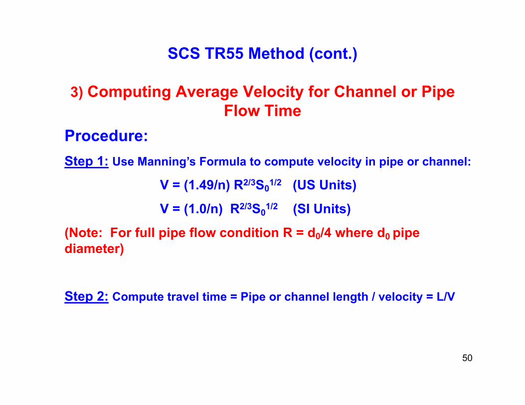
SCS TR55 Method (cont.)
3) Computing Average Velocity for Channel or Pipe Flow Time
Procedure:Step 1: Use Manning’s Formula to compute velocity in pipe or channel:
V = (1.49/n) R2/3S01/2 (US Units)
V = (1.0/n) R2/3S01/2 (SI Units)
(N t F f ll i fl diti R d /4 h d i(Note: For full pipe flow condition R = d0/4 where d0 pipe diameter)
Step 2: Compute travel time = Pipe or channel length / velocity = L/V
50

Example 8: TR-55 Time of Concentration Computation
A 300 acre watershed drains along the path ED→DC→CB→BA shown in the table below. Determine the time of concentration, tc using SCS TR55 method
Hydraulic Path Type of Flow Slope (%) Length (ft)
ED Overland Sheet Flow 5.0 100DC Overland Gutter Flow 1.5 300
(unpaved)CB Pipe Flow (d0 = 24 in; n = 0.015) 1.0 3000BA Open Channel Flow (y = 2 ft; n = 0.02) 0.5 5000
(For a wide rectangular: Hydraulic Radius R = flow depth, y)
Note: The pipe is 24 inches in diameter with a Manning’s n = 0.015The open channel is wide rectangular with main bank flow depth = 2.0 ft. and Manning’s n = 0.020.
51
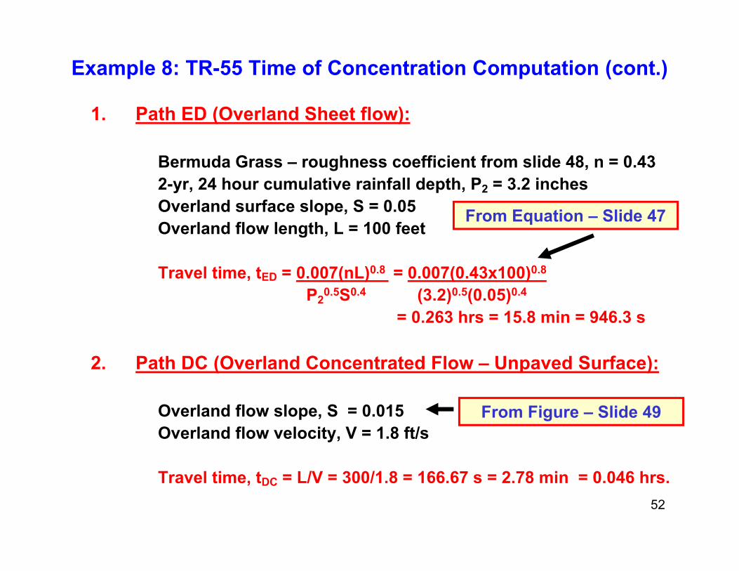
Example 8: TR-55 Time of Concentration Computation (cont.)
1. Path ED (Overland Sheet flow):
Bermuda Grass – roughness coefficient from slide 48, n = 0.432 24 h l i i f ll d h P 3 2 i h2-yr, 24 hour cumulative rainfall depth, P2 = 3.2 inchesOverland surface slope, S = 0.05Overland flow length, L = 100 feet
From Equation – Slide 47
Travel time, tED = 0.007(nL)0.8 = 0.007(0.43x100)0.8
P20.5S0.4 (3.2)0.5(0.05)0.4
= 0.263 hrs = 15.8 min = 946.3 s 0.263 hrs 15.8 min 946.3 s
2. Path DC (Overland Concentrated Flow – Unpaved Surface):
Overland flow slope, S = 0.015Overland flow velocity, V = 1.8 ft/s
From Figure – Slide 49
52
Travel time, tDC = L/V = 300/1.8 = 166.67 s = 2.78 min = 0.046 hrs.
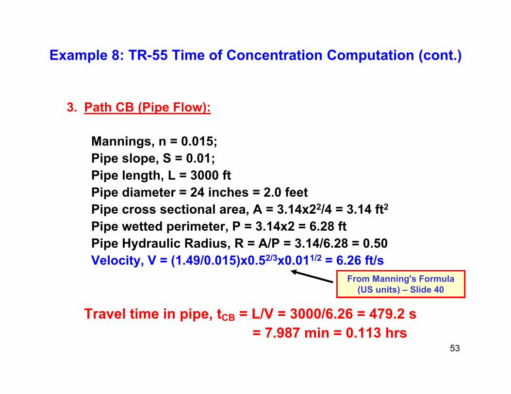
Example 8: TR-55 Time of Concentration Computation (cont.)
3. Path CB (Pipe Flow):
Mannings, n = 0.015; Pipe slope, S = 0.01; Pi l th L 3000 ftPipe length, L = 3000 ftPipe diameter = 24 inches = 2.0 feetPipe cross sectional area, A = 3.14x22/4 = 3.14 ft2
Pi tt d i t P 3 14 2 6 28 ftPipe wetted perimeter, P = 3.14x2 = 6.28 ftPipe Hydraulic Radius, R = A/P = 3.14/6.28 = 0.50Velocity, V = (1.49/0.015)x0.52/3x0.011/2 = 6.26 ft/s
Travel time in pipe, tCB = L/V = 3000/6.26 = 479.2 s
From Manning's Formula (US units) – Slide 40
53= 7.987 min = 0.113 hrs
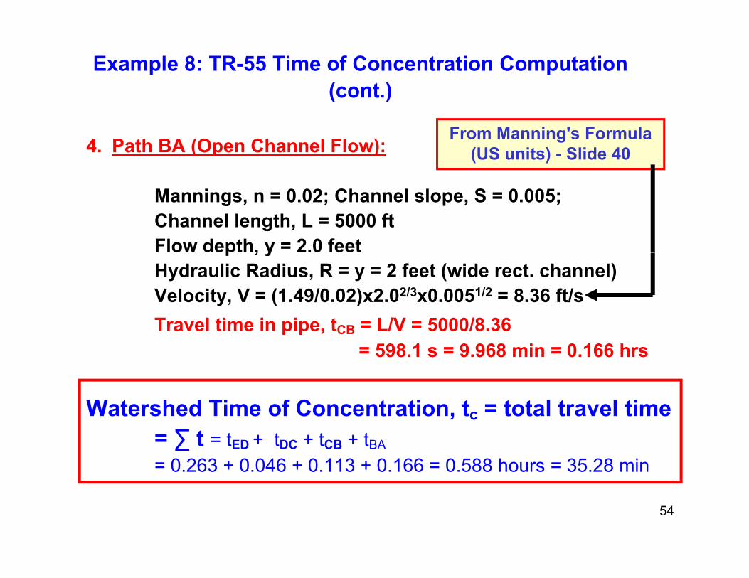
Example 8: TR-55 Time of Concentration Computation (cont.)
4. Path BA (Open Channel Flow):From Manning's Formula
(US units) - Slide 40
Mannings, n = 0.02; Channel slope, S = 0.005; Channel length, L = 5000 ftFlow depth, y = 2.0 feetp , yHydraulic Radius, R = y = 2 feet (wide rect. channel)Velocity, V = (1.49/0.02)x2.02/3x0.0051/2 = 8.36 ft/sTravel time in pipe tCB = L/V = 5000/8 36Travel time in pipe, tCB = L/V = 5000/8.36
= 598.1 s = 9.968 min = 0.166 hrs
Watershed Time of Concentration, tc = total travel time = ∑ t = tED + tDC + tCB + tBA
= 0.263 + 0.046 + 0.113 + 0.166 = 0.588 hours = 35.28 min
54
0.263 0.046 0.113 0.166 0.588 hours 35.28 min
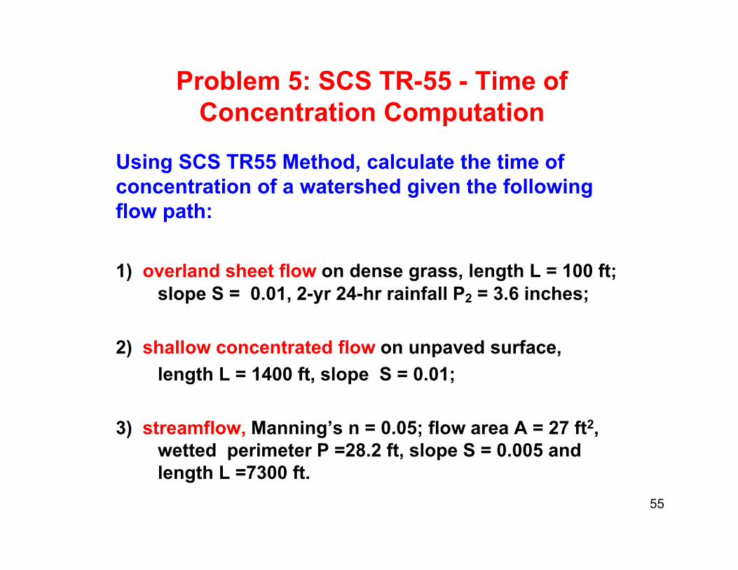
Problem 5: SCS TR-55 - Time of C t ti C t tiConcentration Computation
Using SCS TR55 Method, calculate the time of concentration of a watershed given the following flow path:
1) overland sheet flow on dense grass, length L = 100 ft; slope S = 0.01, 2-yr 24-hr rainfall P2 = 3.6 inches;
2) shallow concentrated flow on unpaved surface, length L = 1400 ft, slope S = 0.01;
3) streamflow, Manning’s n = 0.05; flow area A = 27 ft2, wetted perimeter P =28.2 ft, slope S = 0.005 and
55
length L =7300 ft.
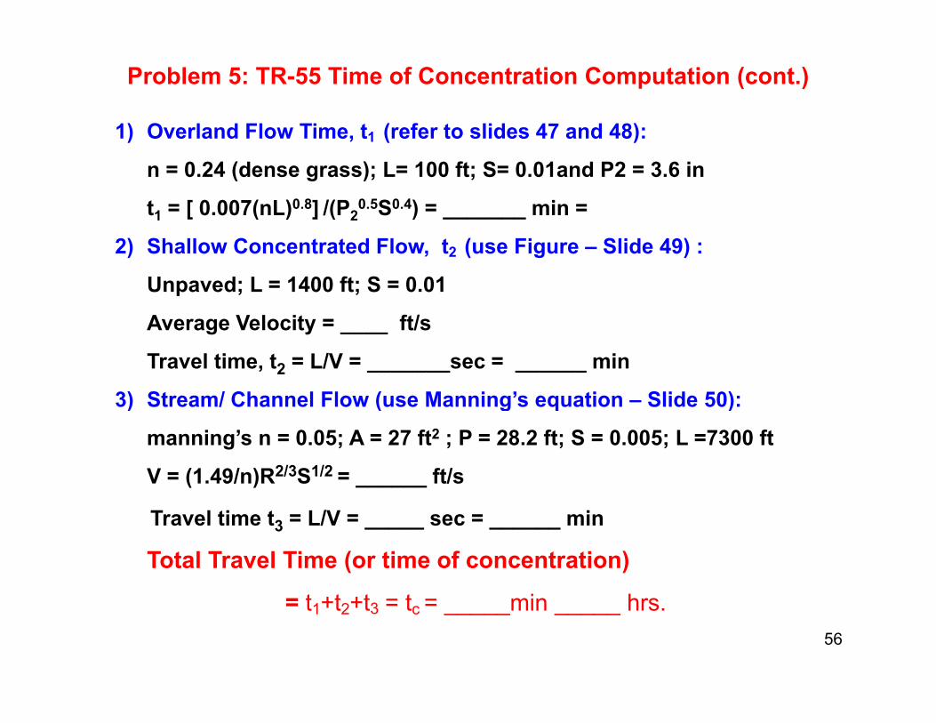
Problem 5: TR-55 Time of Concentration Computation (cont.)
1) Overland Flow Time t1 (refer to slides 47 and 48):1) Overland Flow Time, t1 (refer to slides 47 and 48):
n = 0.24 (dense grass); L= 100 ft; S= 0.01and P2 = 3.6 in
t1 = [ 0.007(nL)0.8] /(P20.5S0.4) = _______ min =
2) Shallow Concentrated Flow, t2 (use Figure – Slide 49) :
Unpaved; L = 1400 ft; S = 0.01
A V l it ft/Average Velocity = ____ ft/s
Travel time, t2 = L/V = _______sec = ______ min
3) Stream/ Channel Flow (use Manning’s equation – Slide 50):) ( g q )
manning’s n = 0.05; A = 27 ft2 ; P = 28.2 ft; S = 0.005; L =7300 ft
V = (1.49/n)R2/3S1/2 = ______ ft/s
Travel time t3 = L/V = _____ sec = ______ min
Total Travel Time (or time of concentration)
56
= t1+t2+t3 = tc = _____min _____ hrs.

SCS TR55 Method – Peak Discharge ComputationComputation
Steps:
1. Compute watershed composite curve number CN;2 Compute sorptivity S (inches) initial abstraction Ia2. Compute sorptivity, S (inches), initial abstraction, Ia
(inches) and Ia/P ratio;3. Compute direct runoff volume Q (inches);4 Compute unit peak discharge q (cfs/sq mi/inch) given4. Compute unit peak discharge, qu (cfs/sq. mi/inch) given
time of concentration, tc and Ia/P ratio from Figure in Slide 58 (or similar curve for Type I and III )
5 Determine the pond factor F5. Determine the pond factor, F.6. Compute peak discharge qp = qu Q A F
57

SCS TR55 Method – Peak Discharge Computation Figure: Unit Peak Discharge Curves-Type IIFigure: Unit Peak Discharge Curves Type II
Refer to USDA TR55 Manual for Type I-A, Type I-B and Type III Curves
58

Example 9: TR-55 Computation of Peak Flow U i SCSTR55 G hi l P k Di h M th dUsing SCSTR55 Graphical Peak Discharge Method
Given:Given:
• 250 acre (0.39 sq. miles) watershed;( q )• 25-year, 24hour Type II design rainfall P = 6 inches;• watershed time of concentration, tc = 1.50 hours;• composite SCS Curve number CN = 75• Neglect storage in lakes and ponds.
Compute the peak discharge qp.
59
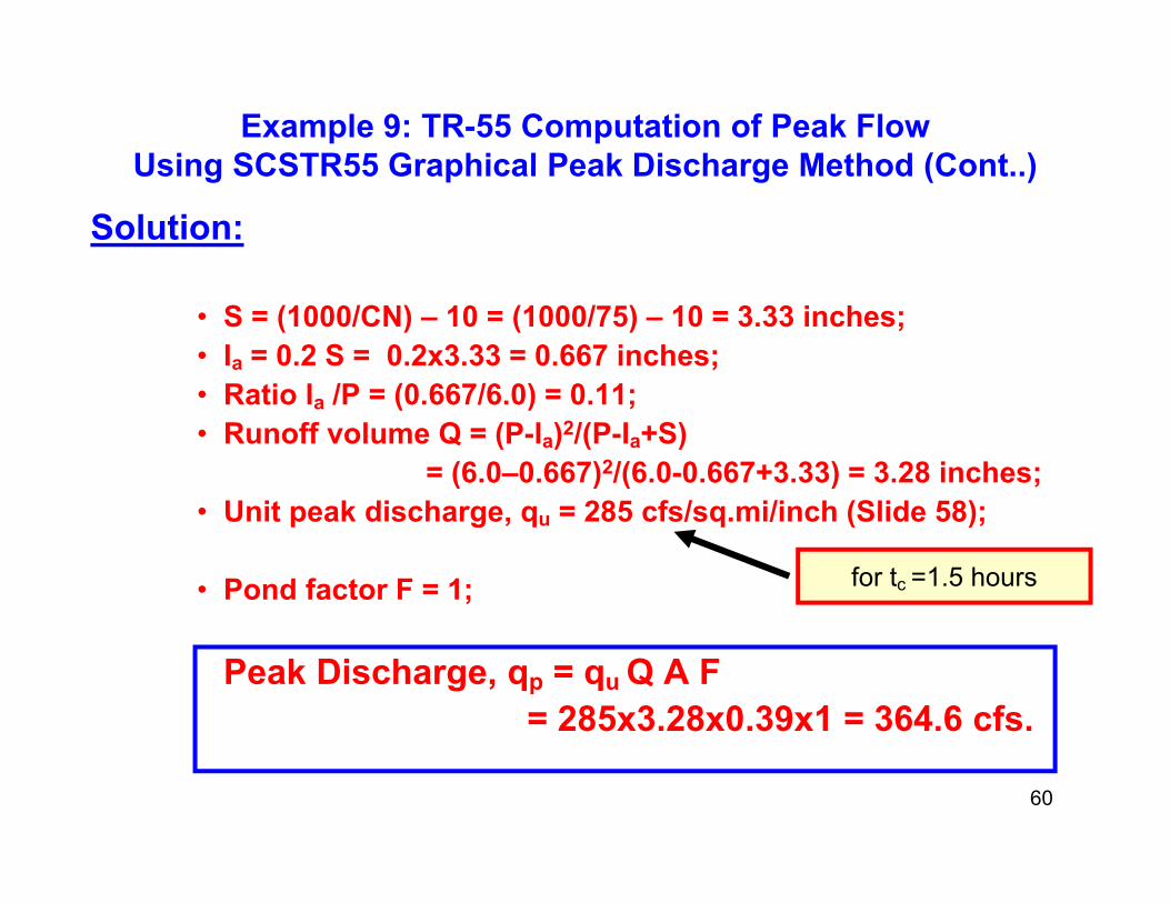
Example 9: TR-55 Computation of Peak Flow Using SCSTR55 Graphical Peak Discharge Method (Cont )Using SCSTR55 Graphical Peak Discharge Method (Cont..)
Solution:
• S = (1000/CN) – 10 = (1000/75) – 10 = 3.33 inches;• Ia = 0.2 S = 0.2x3.33 = 0.667 inches;• Ratio I /P = (0 667/6 0) = 0 11;• Ratio Ia /P = (0.667/6.0) = 0.11;• Runoff volume Q = (P-Ia)2/(P-Ia+S)
= (6.0–0.667)2/(6.0-0.667+3.33) = 3.28 inches;• Unit peak discharge q = 285 cfs/sq mi/inch (Slide 58);• Unit peak discharge, qu = 285 cfs/sq.mi/inch (Slide 58);
• Pond factor F = 1; for tc =1.5 hours
Peak Discharge, qp = qu Q A F = 285x3.28x0.39x1 = 364.6 cfs.
60

Runoff Midsize Catchments Unit Hydrograph MethodUnit Hydrograph Method
• Unit Hydrograph Definition:Unit Hydrograph Definition:The unit hydrograph of a watershed is defined a direct runoff hydrograph (DRH) resulting from 1 inch (or 1 cm in SI units) of excess rainfall generated uniformly over the drainage area at a constant rate for an effective duration tr (referred to as the Unit Hydrograph duration)r ( y g p )
(Adapted from Ponce 1989)
61
Ponce 1989)

Unit Hydrograph Properties(Adapted from Ponce 1989)(Adapted from Ponce 1989)
LinearitySuperposition
Lagging
62

Direct Runoff Convolution (Adapted from Chow el al (1988)
In the equations above:
Pm = rainfall excess pulses (inches or cms)
U it h d h di t f /i 3/ / )
N = M + J - 1Uj = unit hydrograph ordinates cfs/in or m3/s/cms)
Qn = Direct runoff ordinates (cfs)
N = number of non-zero direct runoff ordinates, Qn
63
M = number of rainfall excess pulses in the hyetograph, Pm
J = number of Unit Hydrograph ordinates, Uj
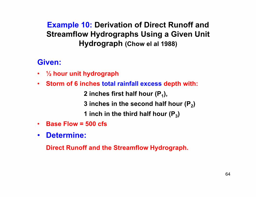
Example 10: Derivation of Direct Runoff and Streamflow Hydrographs Using a Given UnitStreamflow Hydrographs Using a Given Unit
Hydrograph (Chow el al 1988)
Given:Given:• ½ hour unit hydrograph• Storm of 6 inches total rainfall excess depth with: p
2 inches first half hour (P1), 3 inches in the second half hour (P2)1 inch in the third half hour (P3)
• Base Flow = 500 cfs
• Determine:• Determine: Direct Runoff and the Streamflow Hydrograph.
64
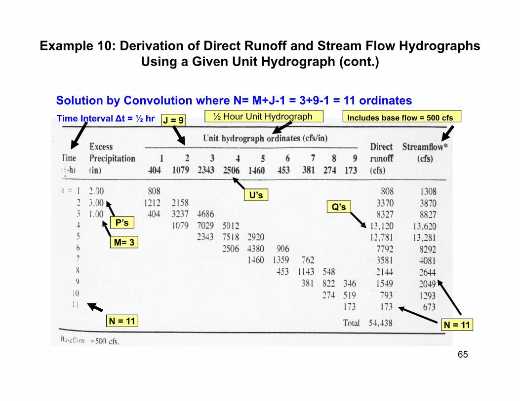
Example 10: Derivation of Direct Runoff and Stream Flow Hydrographs Using a Given Unit Hydrograph (cont.)
Solution by Convolution where N= M+J-1 = 3+9-1 = 11 ordinatesTime Interval Δt = ½ hr Includes base flow = 500 cfsJ = 9 ½ Hour Unit Hydrograph
P’s
U’sQ’s
M= 3
N = 11N = 11
65
N 11
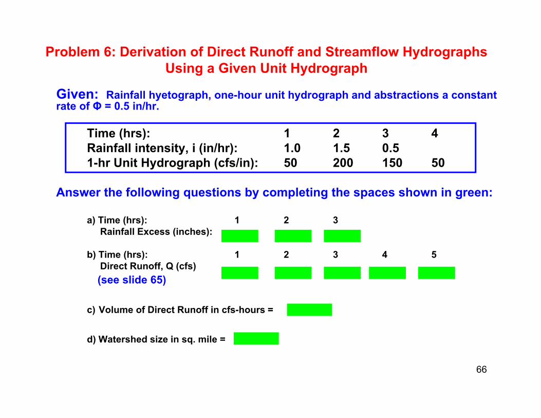
Problem 6: Derivation of Direct Runoff and Streamflow Hydrographs Using a Given Unit Hydrograph
Given: Rainfall hyetograph, one-hour unit hydrograph and abstractions a constant rate of Φ = 0.5 in/hr.
Ti (h ) 1 2 3 4Time (hrs): 1 2 3 4Rainfall intensity, i (in/hr): 1.0 1.5 0.51-hr Unit Hydrograph (cfs/in): 50 200 150 50
Answer the following questions by completing the spaces shown in green:
a) Time (hrs): 1 2 3Rainfall Excess (inches): ( )
b) Time (hrs): 1 2 3 4 5Direct Runoff, Q (cfs)(see slide 65)
c) Volume of Direct Runoff in cfs-hours =
d) Watershed size in sq mile =
66
d) Watershed size in sq. mile

Thank you for listening to the presentationThank you for listening to the presentation.
Remember to Review the following Appendix for:
1. Hydrologic Routing2. Groundwater Hydrology – Well Hydraulicsy gy y3. Additional examples on Unit Hydrograph
Good luck on the P.E. ExamQED
67
QED

REFERENCESREFERENCES1. Chow, Maidment, Mays, 1988. Applied Hydrology
2. Chow, ed. 1964. Handbook of Applied Hydrology
3 Domenico Schwartz 1998 Physical and Chemical Hydrogeology3. Domenico, Schwartz, 1998. Physical and Chemical Hydrogeology.
4. Freeze, Cherry, 1979. Groundwater
5. Maidment, ed. 1993. Handbook of Hydrology
6. Ponce, 1989. Engineering Hydrology
68

Answers• Problem 1 (Slide 9): 1) a; 2) a . • Problem 1 (Slide 10): 3) b; 4) c; 5) b; 6) c .• Problem 2 (Slide 21): 1) b; 2) d; 3) c.• Problem 3 (Slide 34): 1) c; 2) b; 3) d; 4) d• Problem 3 (Slide 34): 1) c; 2) b; 3) d; 4) d.• Problem 4 (Slide 44); 1) c; 2) c; 3) d.• Problem 5 (Slide 55): 1) Overland sheet flow: 0.296 hrs;
2) Overland Shallow Concentrated flow: 0.229 hrs3) Stream Flow: 0.991 hrs4) Total Time of Concentration = 1.515 hours.
• Problem 6 (Slide 66): a) Time (hrs): 1 2 3
• Rainfall excess (inches): 0.5 1.0 0 (M=2)
• b) Time (hrs): 1 2 3 4 5
• Direct runoff (cfs): 25 150 275 175 50 (N=5)
) V l f di t ff V 675 f h 2430 000 ft3• c) Volume of direct runoff, Vd = 675 cfs-hours = 2430,000 ft3
• d) Drainage Area = 0.697 sq. miles
• (Hint: use volume under unit hydrograph = 1 inch or Volume under direct runoff hydrograph
69
y g p

APPENDIX A
Hydrologic Design y g gComponents for
SCS TR55SCS TR55
70

Table: Design Frequency or Return Period for Various Hydraulic Structures
71
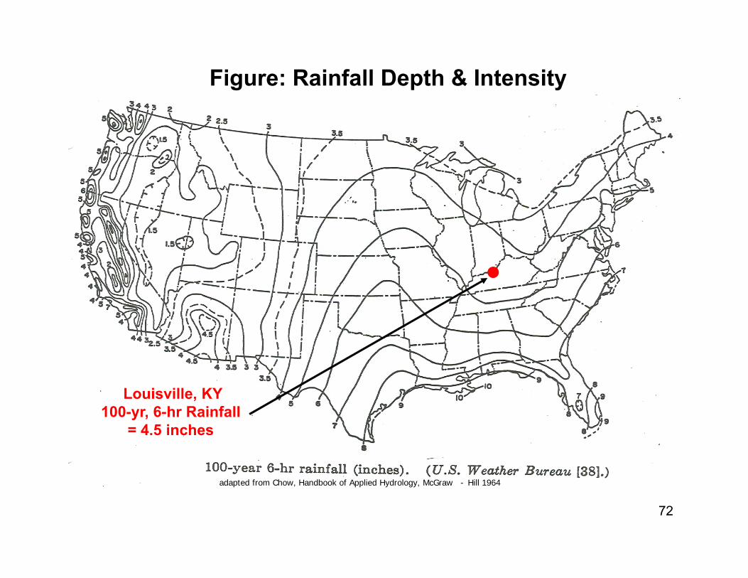
Figure: Rainfall Depth & Intensity
Louisville, KY
40
Louisville, KY100-yr, 6-hr Rainfall
= 4.5 inches
72
adapted from Chow, Handbook of Applied Hydrology, McGraw - Hill 1964
Methods for Computing Time of Concentration
• Formulas
– Example: Kirpich, SCS Average Velocity Charts
• Approximate Velocities
73
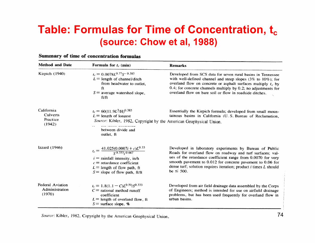
Table: Formulas for Time of Concentration, tc(source: Chow et al, 1988)(source: Chow et al, 1988)
74
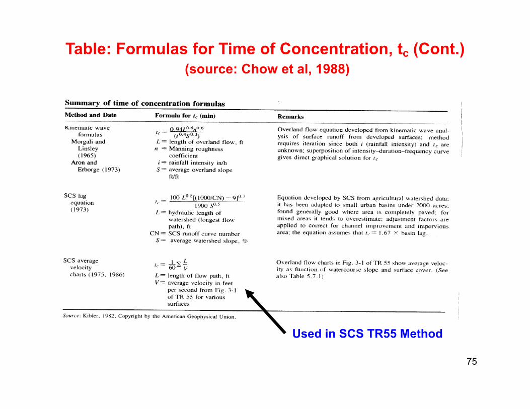
Table: Formulas for Time of Concentration, tc (Cont.)(source: Chow et al, 1988)( )
Used in SCS TR55 Method
75
Used in SCS TR55 Method

Table: Average Velocities for Different Flow Paths(source: Chow et al, 1988)
76
APPENDIX BAPPENDIX B
Hydrologic Routing
77
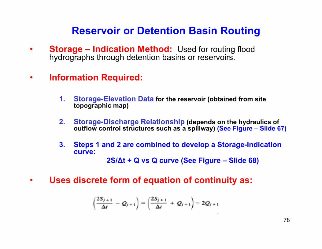
Reservoir or Detention Basin RoutingSt I di ti M th d• Storage – Indication Method: Used for routing flood hydrographs through detention basins or reservoirs.
• Information Required:• Information Required:
1. Storage-Elevation Data for the reservoir (obtained from site topographic map)p g p p)
2. Storage-Discharge Relationship (depends on the hydraulics of outflow control structures such as a spillway) (See Figure – Slide 67)
3. Steps 1 and 2 are combined to develop a Storage-Indication curve:
2S/Δt + Q vs Q curve (See Figure – Slide 68)
• Uses discrete form of equation of continuity as:
78
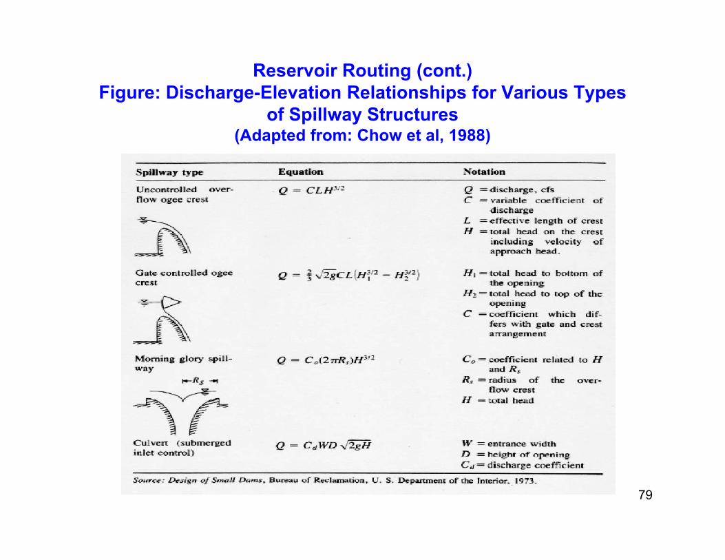
Reservoir Routing (cont.)Figure: Discharge-Elevation Relationships for Various Types
of Spillway Structures (Adapted from: Chow et al, 1988)
79

Reservoir Routing (cont.) Figure: Development of Storage Indication Curve
(Chow et al, 1988)
80

Reservoir Routing (cont.)Example 8: Developing a Storage Indication Curve.
Problem Statement:Storage vs outflow characteristics for a proposed reservoir are given below.Storage vs outflow characteristics for a proposed reservoir are given below. Calculate the storage-outflow function 2S/Δt + Q vs Q for each of the tabulated values if Δt = 2 hours. Plot a graph of the storage-outflow function.
________________________________________________________________________St S (106 3) 75 81 87 5 100 110 2Storage, S (106 m3): 75 81 87.5 100 110.2
Outflow, Q (m3/s): 57 227 519 1330 2270
________________________________________________________________________
Solution:
81
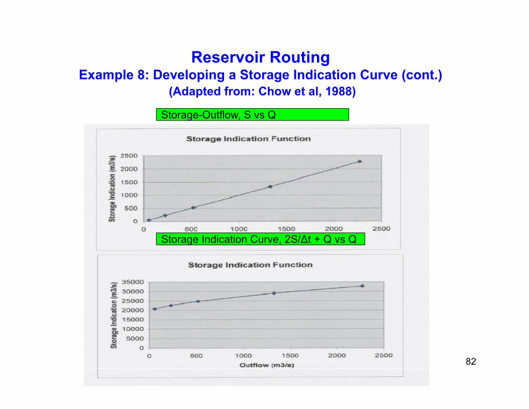
Reservoir Routing Example 8: Developing a Storage Indication Curve (cont )Example 8: Developing a Storage Indication Curve (cont.)
(Adapted from: Chow et al, 1988)
Storage-Outflow, S vs Q
Storage Indication Curve, 2S/Δt + Q vs Q
82
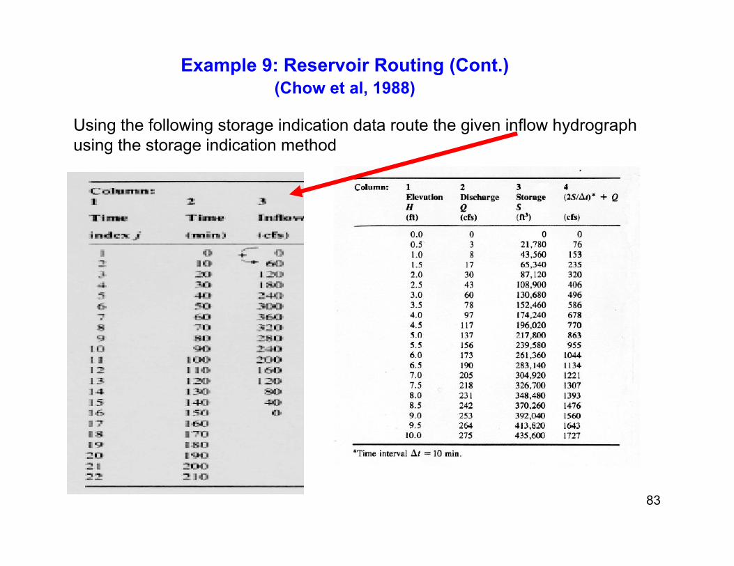
Example 9: Reservoir Routing (Cont.)(Chow et al, 1988)
Using the following storage indication data route the given inflow hydrograph using the storage indication method
83

Example 9 Reservoir Routing (Chow et al, 1988) (cont.):
Solution:From Storage Indication Equation
(2Sj+1/Δt + Qj+1) = (Ij+1 + Ij) + (2Sj/Δt - Qj)
From Storage Indication Curve Table Slide 73
outflow hydrograph
inflow hydrograph
Solve this equation for t ti t j 3
84
next time step j = 3
Column 5 Column 6
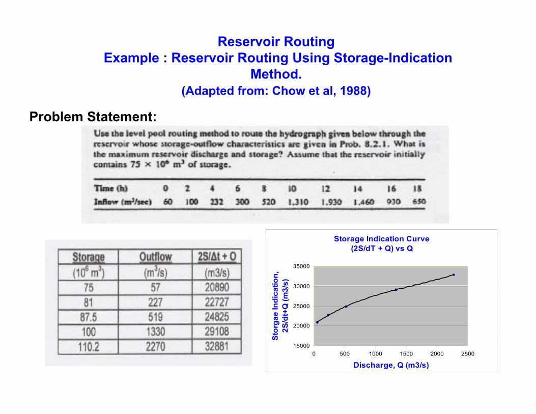
Reservoir Routing Example : Reservoir Routing Using Storage-Indication
MethodMethod. (Adapted from: Chow et al, 1988)
Problem Statement:
Storage Indication Curve(2S/dT + Q) vs Q
30000
35000
tion,
s)
20000
25000
30000
Stor
gae
Indi
cat
2S/d
t+Q
(m3/
s
85
150000 500 1000 1500 2000 2500
Discharge, Q (m3/s)
S
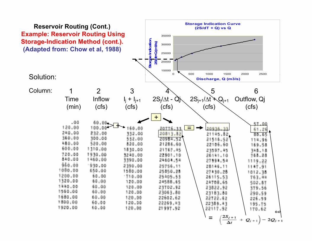
Reservoir Routing (Cont.)Example: Reservoir Routing Using Storage-Indication Method (cont.).
Storage Indication Curve(2S/dT + Q) vs Q
30000
35000
tion,
/s)g ( )
(Adapted from: Chow et al, 1988)
S l ti15000
20000
25000
30000
0 500 1000 1500 2000 2500
Stor
gae
Indi
cat
2S/d
t+Q
(m3/
1 2 3 4 5 6 Time Inflow Ij + Ij+1 2Sj/∆t - Qj 2Sj+1/∆t + Qj+1 Outflow, Qj( i ) ( f ) ( f ) ( f ) ( f ) ( f )
Solution:
Column:
Discharge, Q (m3/s)
(min) (cfs) (cfs) (cfs) (cfs) (cfs)
+=+
86=
APPENDIX CAPPENDIX C
Groundwater: Well HydraulicsWell Hydraulics
87
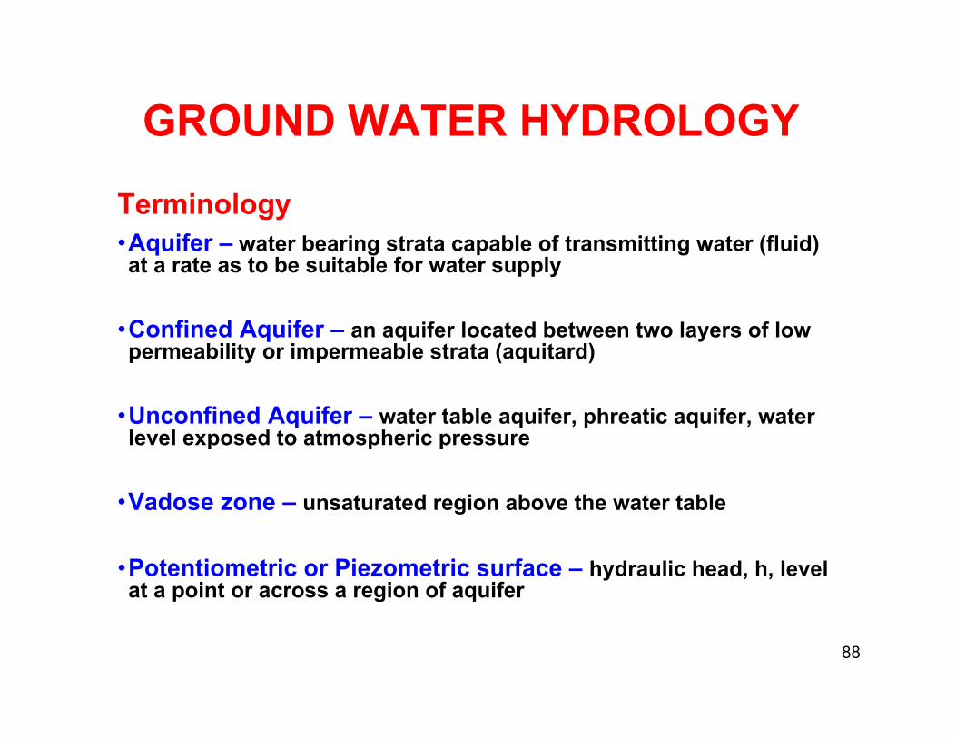
GROUND WATER HYDROLOGY
Terminology•Aquifer – water bearing strata capable of transmitting water (fluid) at a rate as to be suitable for water supply
C fi d A if if l t d b t t l f l•Confined Aquifer – an aquifer located between two layers of low permeability or impermeable strata (aquitard)
•Unconfined Aquifer water table aquifer phreatic aquifer water•Unconfined Aquifer – water table aquifer, phreatic aquifer, water level exposed to atmospheric pressure
•Vadose zone – unsaturated region above the water tableVadose zone unsaturated region above the water table
•Potentiometric or Piezometric surface – hydraulic head, h, level at a point or across a region of aquiferg
88

Fundamental Principles
Darcy’s Law: q = K iq ≡ specific discharge {L/T}q ≡ specific discharge {L/T}K ≡ hydraulic conductivity {L/T},
(ft/s, m/s)i ≡ hydraulic gradient = dh/dL
{dimensionless, L/L}
h = hydraulic head, h = ψ + zψΨ ≡ gage pressure head or water
pressure = pgage/γ {L}z ≡ elevation head {L}
Note: Ψ = 0 in saturated zone
z ≡ elevation head {L}
89
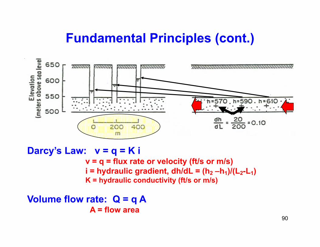
Fundamental Principles (cont.)
Darcy’s Law: v = q = K iv = q = flux rate or velocity (ft/s or m/s)i = hydraulic gradient dh/dL = (h h )/(L L )i = hydraulic gradient, dh/dL = (h2 –h1)/(L2-L1)K = hydraulic conductivity (ft/s or m/s)
Volume flow rate: Q = q AVolume flow rate: Q q AA = flow area
90
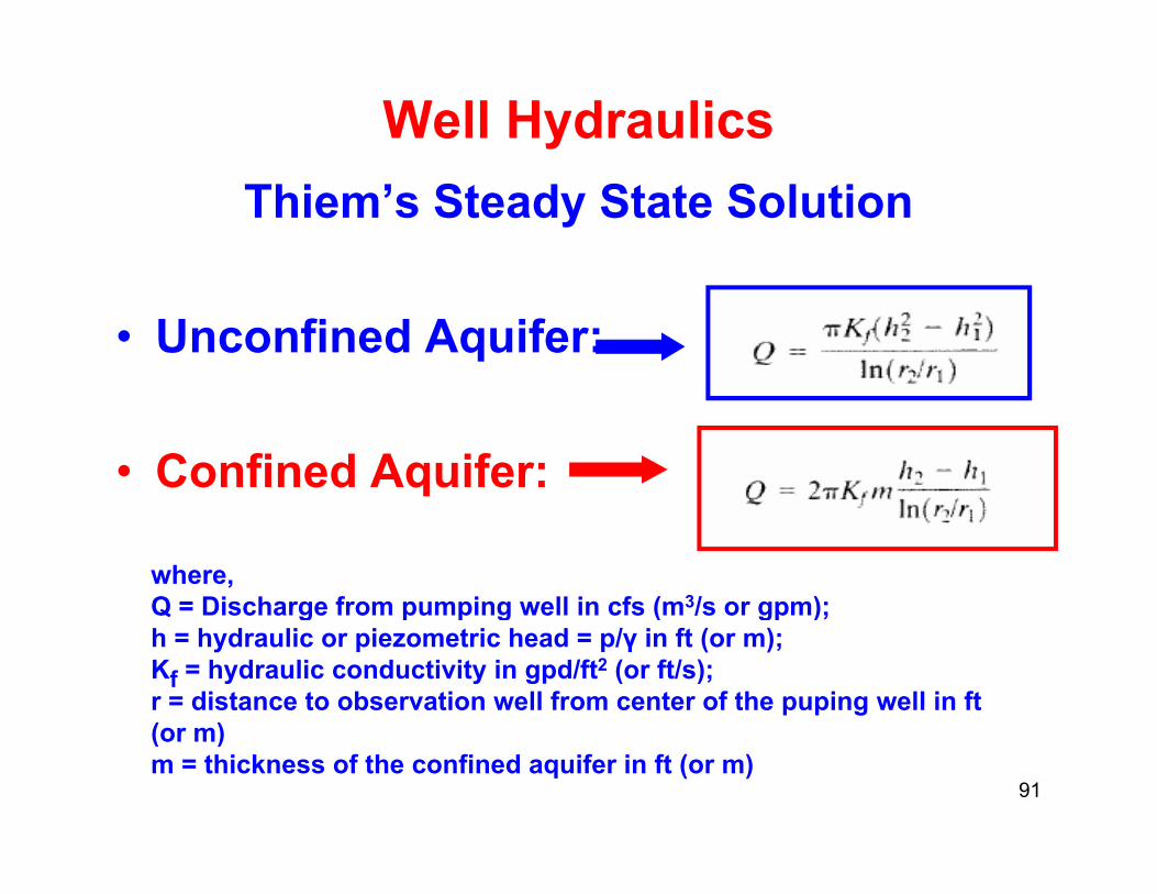
Well HydraulicsThiem’s Steady State Solution
• Unconfined Aquifer:
• Confined Aquifer:
where,Q = Discharge from pumping well in cfs (m3/s or gpm);Q g p p g ( gp );h = hydraulic or piezometric head = p/γ in ft (or m);Kf = hydraulic conductivity in gpd/ft2 (or ft/s);r = distance to observation well from center of the puping well in ft (or m)(or m)m = thickness of the confined aquifer in ft (or m)
91

Example: Thiem’s Steady State Solution - Unconfined AquiferAquifer
92

Example: Thiem’s Steady State Solution - Unconfined AquiferSolution Unconfined Aquifer
Given:
•A 20 inch diameter well fully penetrates a 100 ft deep unconfined aquifer;•Drawdowns at two observation wells located at 90 ft and 240 ft from the pumping well are 23 ft and 21.5 ft respectively;the pumping well are 23 ft and 21.5 ft respectively; •Hydraulic Conductivity of the aquifer is Kf = 1400 gpd/ft2 x ((1.55x10⁻⁶
cfs/gpd) = 2.17x10⁻³ ft/s•Determine: The discharge Q from the pumping well in gpm
Solution:Hydraulic heads: h1 = 100 – 23 = 77 ft (at r1 = 90 ft);
h2 = 100 – 21 5 = 78 5 ft (at r2 = 240 ft);h2 = 100 – 21.5 = 78.5 ft. (at r2 = 240 ft);Kf = 1400 gpd/ft2 x ((1.55x10⁻⁶ cfs/gpd) = 2.17x10⁻³ ft/s
Q = 3.14 K f (h22 – h1
2) / loge(r2/r1) - all in consistent units3 2 2
93
= 3.14 x 2.17x10-3 ( 78.52 – 772 ) / loge(240/90)= 1.62 cfs = 725.9 gpm
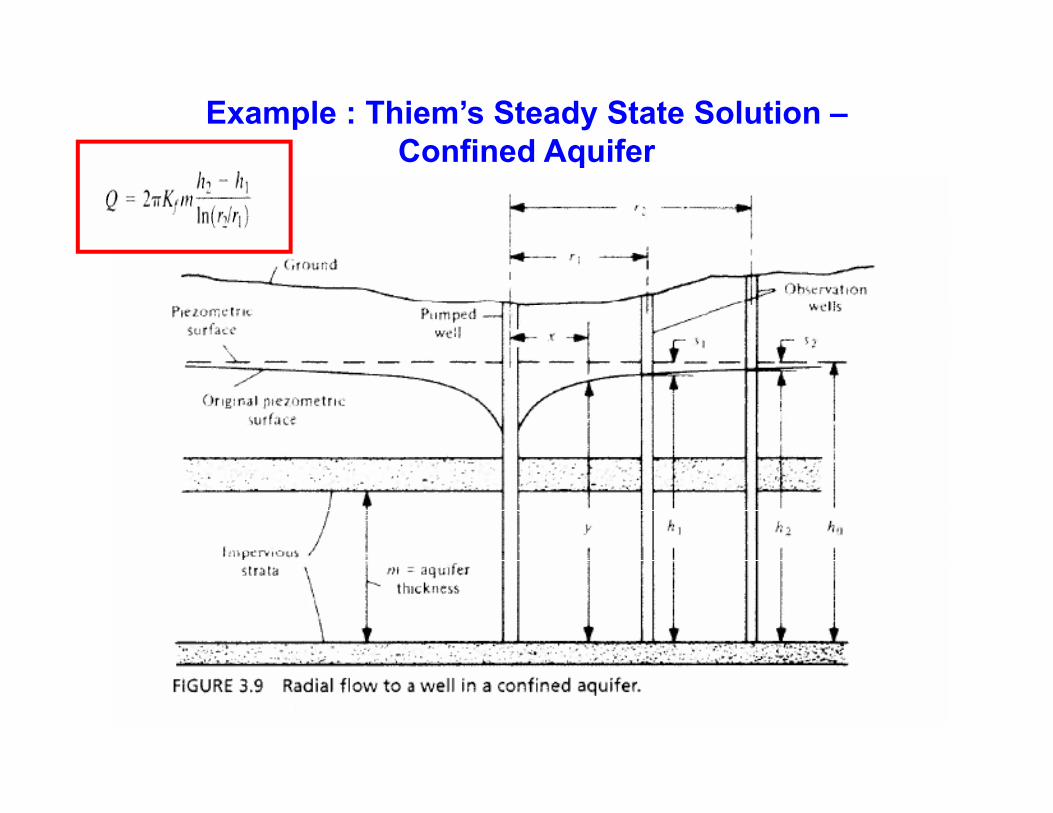
Example : Thiem’s Steady State Solution –Confined AquiferConfined Aquifer
94

Example : Thiem’s Steady State Solution –Confined AquiferConfined Aquifer
Problem: Determine the hydraulic conductivity, Kf , of an artesian aquifer (confined aquifer) pumped by a fully penetrating well. GiGiven:
1) Aquifer thickness, m = 100 feet2) Steady state pumping rate Q =1000 gpm = 2.232 cfs3) Drawdowns s at observation wells:3) Drawdowns, s, at observation wells:
Well 1: r1 = 50 ft; s1 = 10 (h1 = 100-10 = 90 ft)Well 2: r2 = 500 ft; s2 = 1 ft (h2 = 100-1= 99 ft)
Solution:Solution:Solve for Hydraulic Conductivity, Kf from Thiem’ssteady state equation for confined aquifer:
Kf = {Q (loge(r2/r1) }/ {(2 ∏ m (h2 – h1)} - all in consistent units= {2.232xloge(500/50)}/{2x3.14x100x(99-90)}= 9.093x10⁻⁴ ft/s or ft3/s.ft2
95
= (9.093x10⁻⁴ft3/s.ft2) x 646,323 gpd/ft2
= 587.7 gpd/ft2
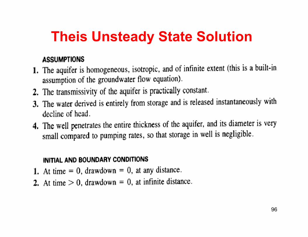
Theis Unsteady State Solutiony
96
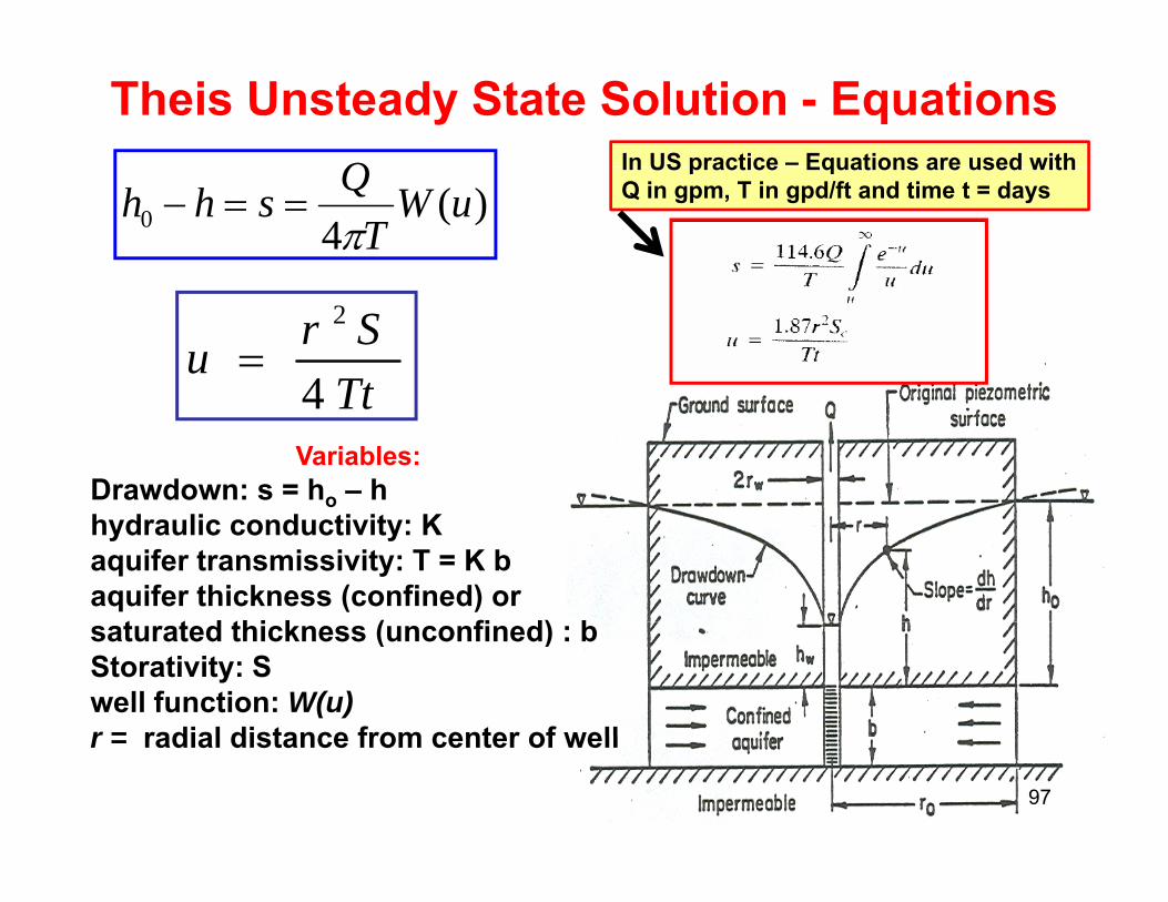
Theis Unsteady State Solution - EquationsQ In US practice – Equations are used with
)(40 uW
TQshhπ
==−In US practice Equations are used with Q in gpm, T in gpd/ft and time t = days
TtSru
4
2
=Tt4
Variables:Drawdown: s = ho – h hydraulic conductivity: K aquifer transmissivity: T = K baquifer thickness (confined) or
t t d thi k ( fi d) bsaturated thickness (unconfined) : bStorativity: S well function: W(u)r = radial distance from center of wellr = radial distance from center of well
97
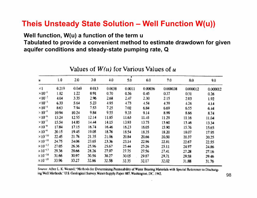
Well function, W(u) a function of the term u
Theis Unsteady State Solution – Well Function W(u))Well function, W(u) a function of the term uTabulated to provide a convenient method to estimate drawdown for given aquifer conditions and steady-state pumping rate, Q
98

Example: Theis MethodGiven: A well is pumped at Q = 5400 m3/dayAquifer properties:Aquifer properties: S = 0.0003; T = 2200 m2/day (0.0025 m2/s)C tCompute: Drawdown, s = h0-h , at t = 10 days, r = 20 m
Solution:Compute u = 1.36.10-6
Well Function: W(u) = 12.99( )
)(40 uW
TQshhπ
==−
Drawdown, s = {5400/(4x3.14x2200)} x 12.99 = 2.53 m99
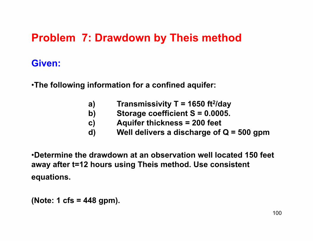
Problem 7: Drawdown by Theis method
Given:
•The following information for a confined aquifer:
a) Transmissivity T = 1650 ft2/daya) Transmissivity T 1650 ft /day b) Storage coefficient S = 0.0005.c) Aquifer thickness = 200 feet d) Well delivers a discharge of Q = 500 gpm) g gp
•Determine the drawdown at an observation well located 150 feet away after t=12 hours using Theis method. Use consistentaway after t 12 hours using Theis method. Use consistent equations.
100
(Note: 1 cfs = 448 gpm).

APPENDIX DAPPENDIX D
Unit Hydrograph
Additional ExamplesAdditional Examples
101
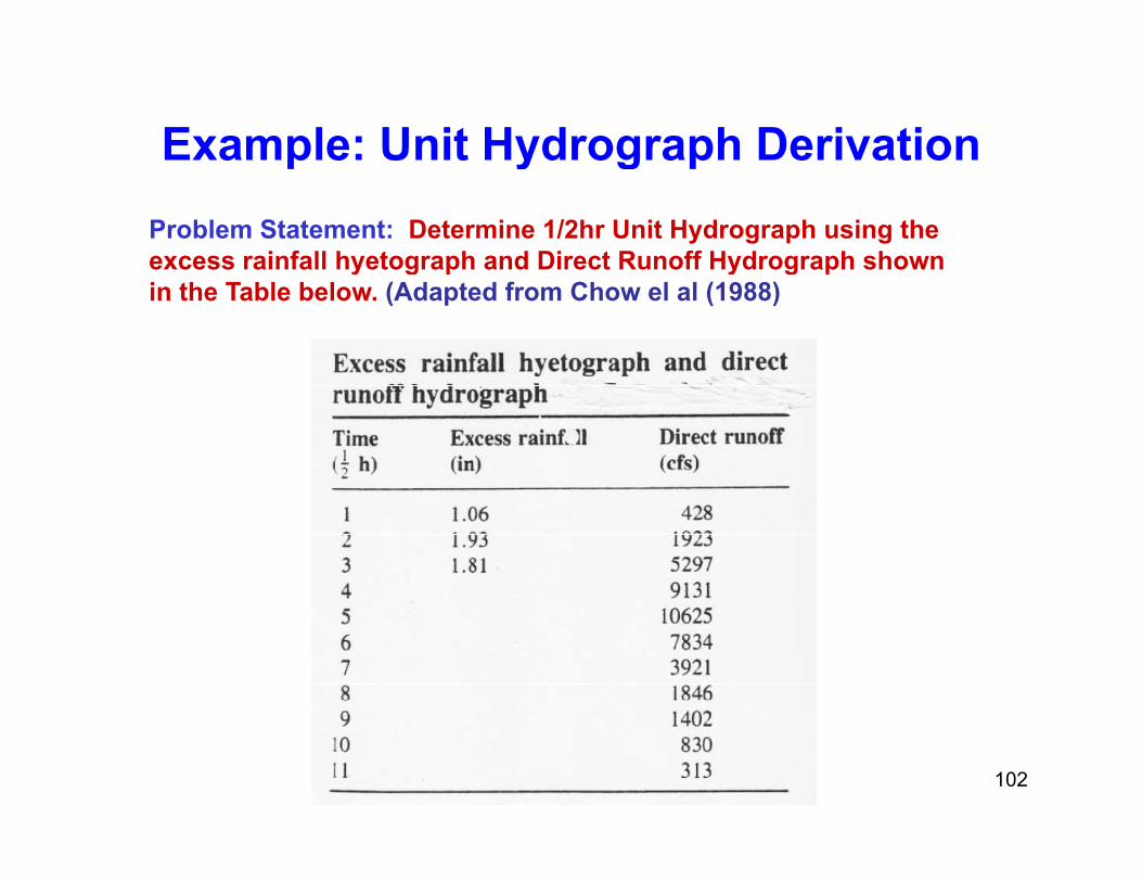
Example: Unit Hydrograph Derivationp y g pProblem Statement: Determine 1/2hr Unit Hydrograph using the excess rainfall hyetograph and Direct Runoff Hydrograph shown y g p y g pin the Table below. (Adapted from Chow el al (1988)
102
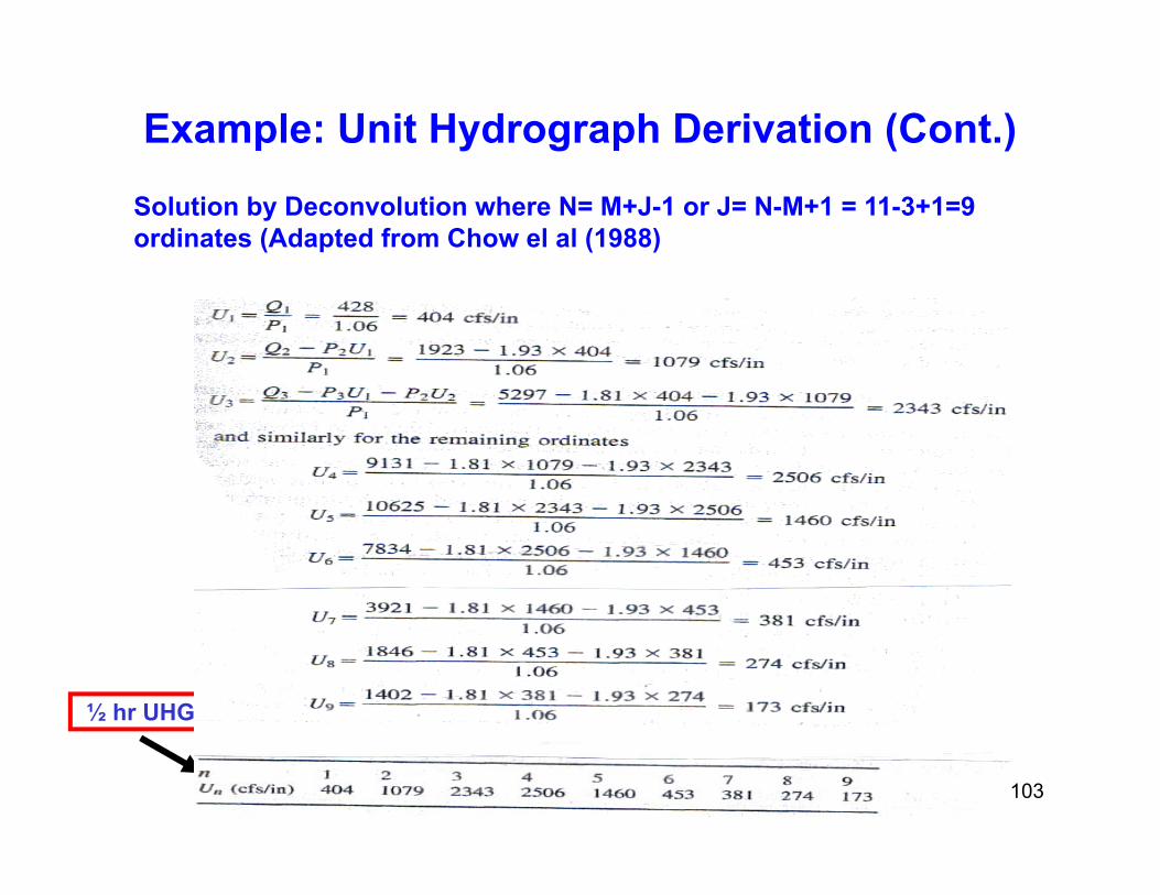
Example: Unit Hydrograph Derivation (Cont.)
Solution by Deconvolution where N= M+J-1 or J= N-M+1 = 11-3+1=9 ordinates (Adapted from Chow el al (1988)
½ hr UHG
103
Problem : Derivation of Direct Runoff and StreamflowHydrographs Using a Given Unit Hydrograph
Problem Statement:
104
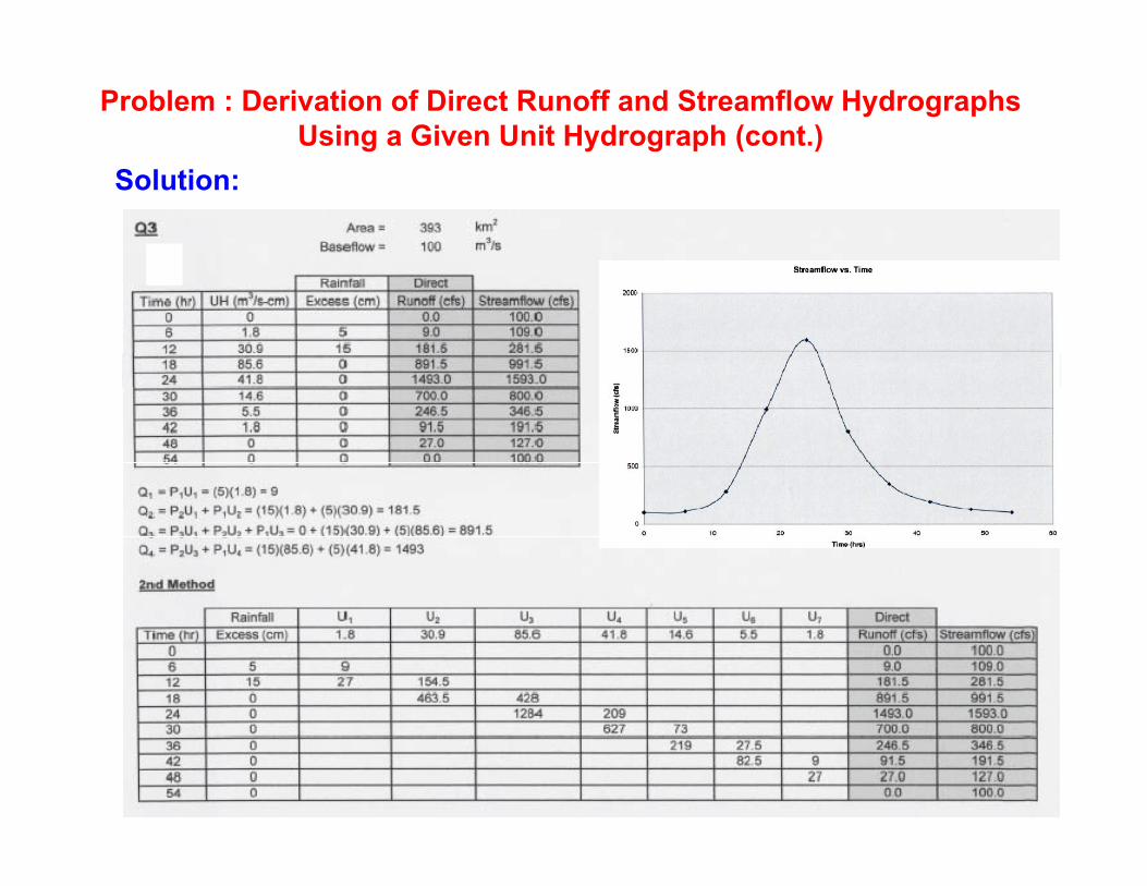
Problem : Derivation of Direct Runoff and Streamflow Hydrographs Using a Given Unit Hydrograph (cont.)
Solution:
105
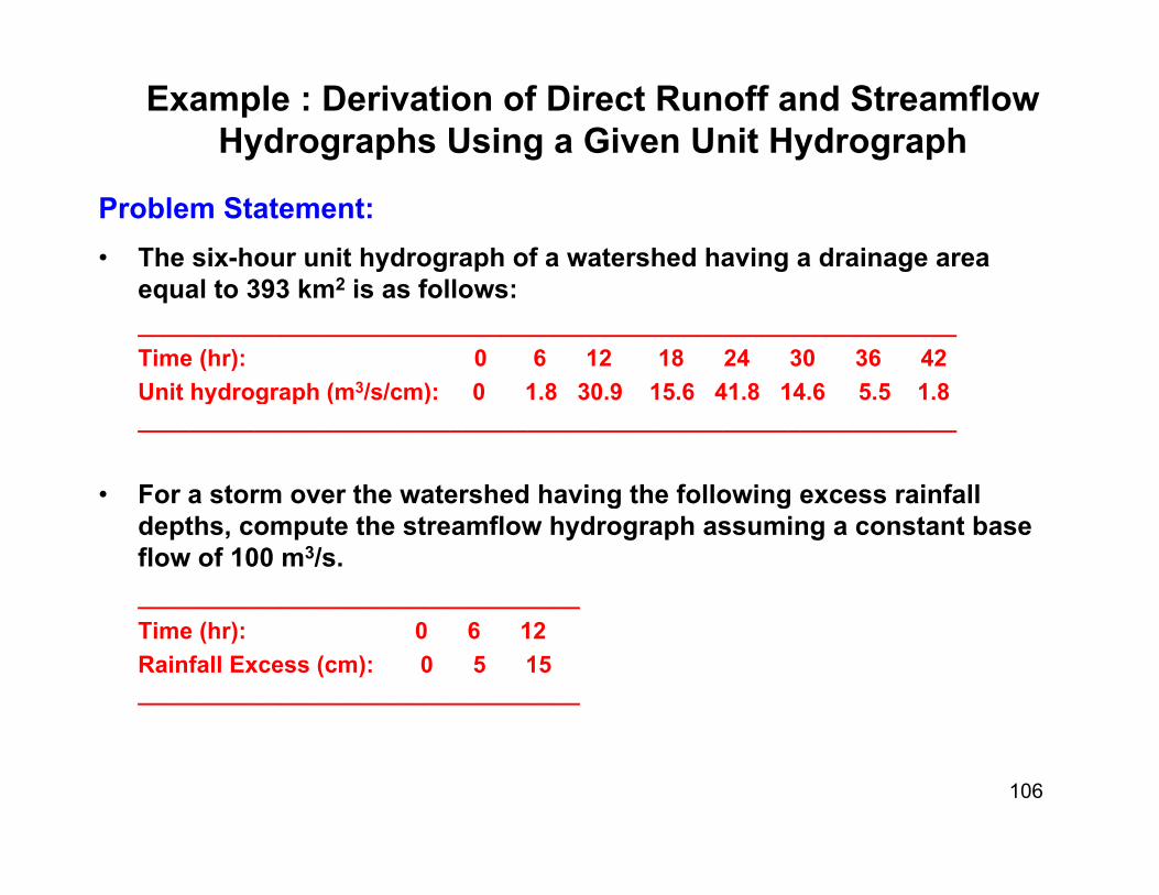
Example : Derivation of Direct Runoff and StreamflowHydrographs Using a Given Unit Hydrograph
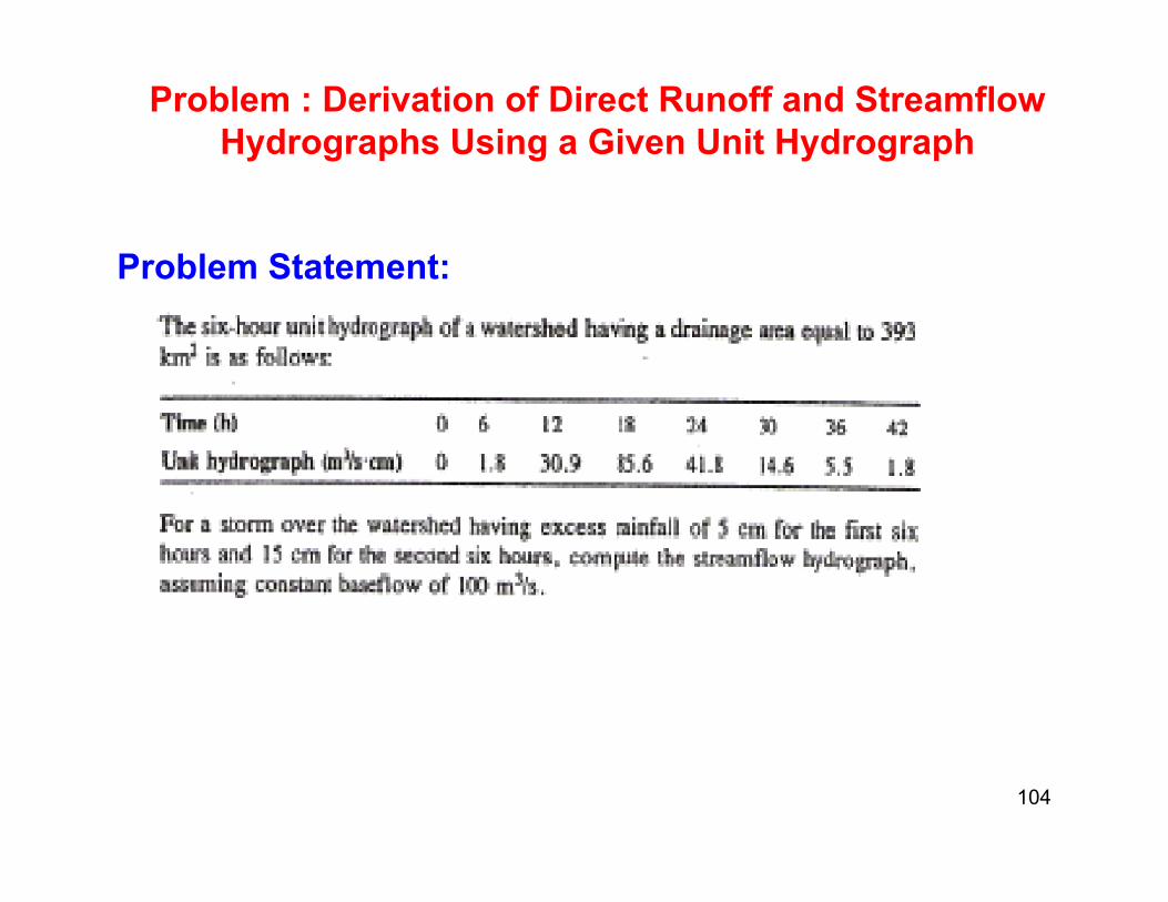
Problem Statement:• The six-hour unit hydrograph of a watershed having a drainage area
2equal to 393 km2 is as follows:_______________________________________________________________Time (hr): 0 6 12 18 24 30 36 42Unit hydrograph (m3/s/cm): 0 1 8 30 9 15 6 41 8 14 6 5 5 1 8Unit hydrograph (m3/s/cm): 0 1.8 30.9 15.6 41.8 14.6 5.5 1.8_______________________________________________________________
• For a storm over the watershed having the following excess rainfall g gdepths, compute the streamflow hydrograph assuming a constant base flow of 100 m3/s.__________________________________Time (hr): 0 6 12 Rainfall Excess (cm): 0 5 15__________________________________
106

Example: Derivation of Direct Runoff and Streamflow Hydrographs Using a Given Unit Hydrograph (cont.)
Solution:
107

Example: Unit Hydrograph Derivationp y g pProblem Statement: Determine 1/2hr Unit Hydrograph using the excess rainfall hyetograph and Direct Runoff Hydrograph shown y g p y g pin the Table below. (Adapted from Chow el al (1988)
108
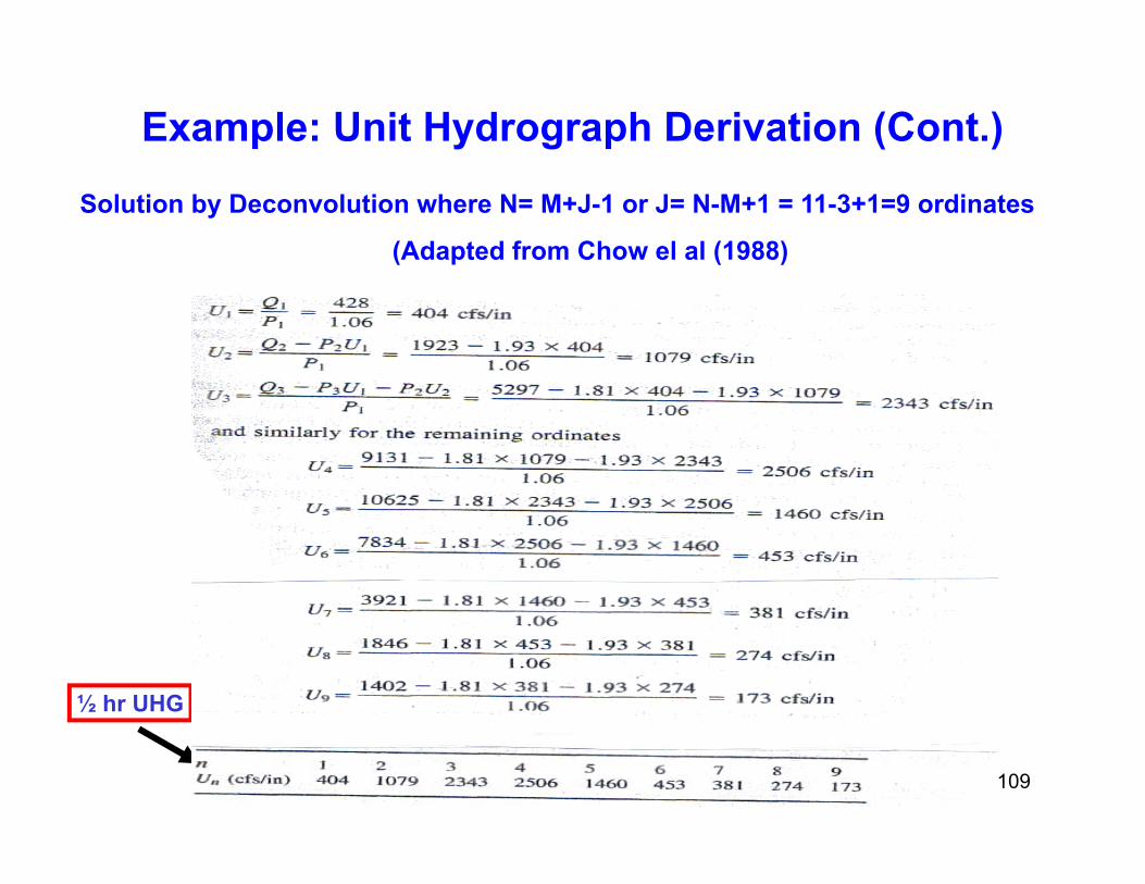
Example: Unit Hydrograph Derivation (Cont.)
Solution by Deconvolution where N= M+J-1 or J= N-M+1 = 11-3+1=9 ordinates
(Adapted from Chow el al (1988)
½ hr UHG
109