Embed Size (px)
Citation preview

7/21/2019 Pe Civil Hydrology Fall 2011
http://slidepdf.com/reader/full/pe-civil-hydrology-fall-2011 1/109
P.E. Civil Exam Review:
N.R. Bhaskar
Email: bhaskar louisville.edu
Phone: 502-852-4547
7/21/2019 Pe Civil Hydrology Fall 2011
http://slidepdf.com/reader/full/pe-civil-hydrology-fall-2011 2/109
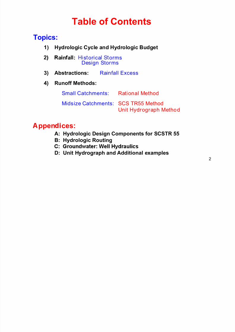
Table of Contents
Topics:
1) Hydrologic Cycle and Hydrologic Budget
a n a : s or ca orms
Design Storms
3) Abstractions: Rainfall Excess
4) Runoff Methods:
Small Catchments: Rational Method
Midsize Catchments: SCS TR55 Method
Unit Hydrograph Method
ppen ces:A: Hydrologic Design Components for SCSTR 55
B: Hydrologic Routing
2
D: Unit Hydrograph and Additional examples

7/21/2019 Pe Civil Hydrology Fall 2011
http://slidepdf.com/reader/full/pe-civil-hydrology-fall-2011 3/109
Hydrologic Cycle and Terms
• Precipitation/Rainfall.
Discharge of water
from the atmosphere.
• .
Rainfall minus interception
depression storageevapora on
infiltration
• Runoff.
(includes subsurface quick return flow).
3
• ur ace runo .
Runoff which travels over the soil surface to the nearest stream.
7/21/2019 Pe Civil Hydrology Fall 2011
http://slidepdf.com/reader/full/pe-civil-hydrology-fall-2011 4/109
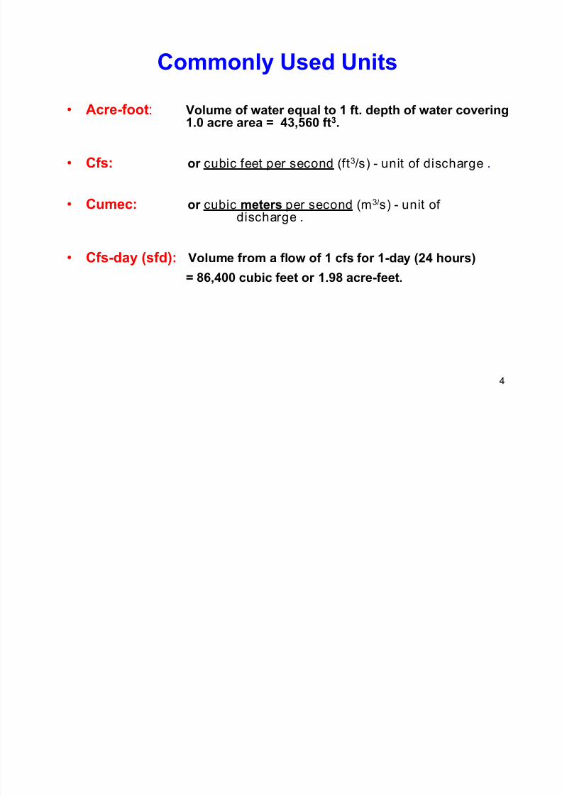
Commonly Used Units
• Acre-foot: Volume of water equal to 1 ft. depth of water covering1.0 acre area = 43,560 ft3.
• Cfs: or cubic feet per second (ft3/s) - unit of discharge .
• Cumec: or cubic meters per second (m3/s) - unit ofdischarge .
• Cfs-day (sfd): Volume from a flow of 1 cfs for 1-day (24 hours)
= 86,400 cubic feet or 1.98 acre-feet.
4
7/21/2019 Pe Civil Hydrology Fall 2011
http://slidepdf.com/reader/full/pe-civil-hydrology-fall-2011 5/109
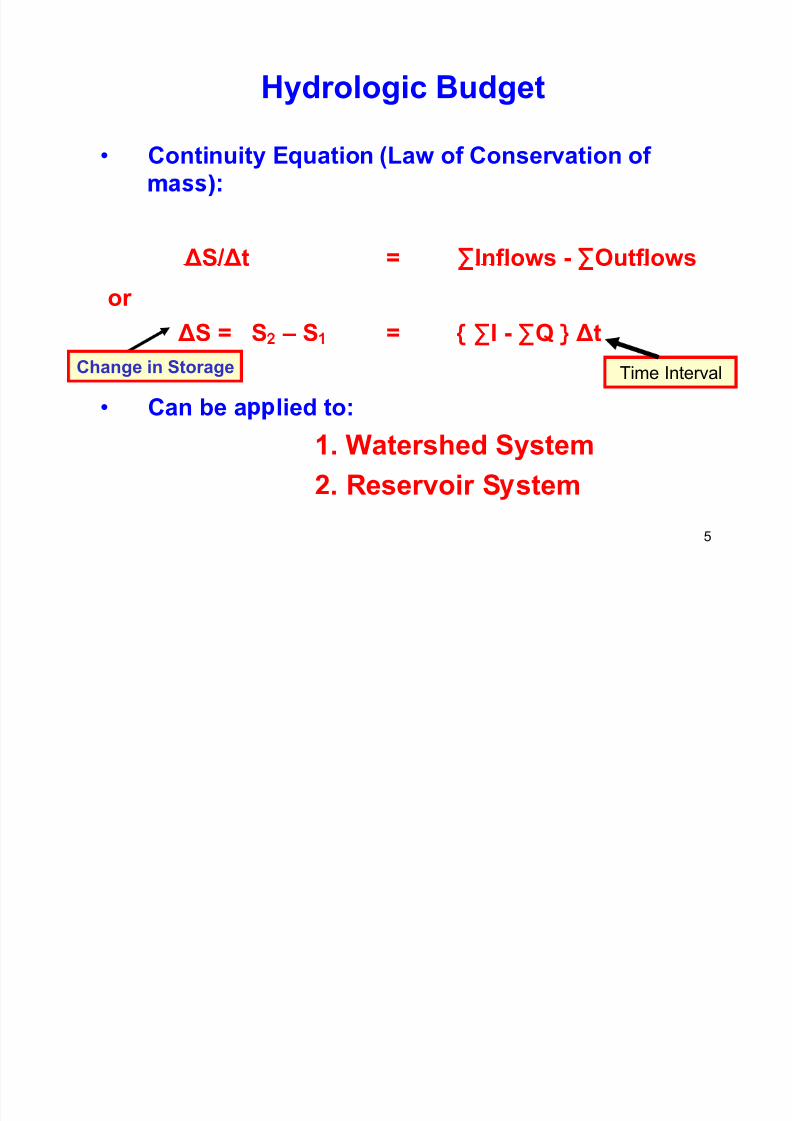
Hydrologic Budget
• Continuity Equation (Law of Conservation of
ΔS/Δt = Inflows - Outflows
or
ΔS = S – S = I - Q Δt
• Can be a lied to:
Change in Storage Time Interval
1. Watershed System
2. Reservoir S stem
5
7/21/2019 Pe Civil Hydrology Fall 2011
http://slidepdf.com/reader/full/pe-civil-hydrology-fall-2011 6/109
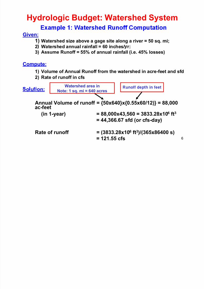
Hydrologic Budget: Watershed System
Given:
1) Watershed size above a gage site along a river = 50 sq. mi;
2 Watershed annual rainfall = 60 inches/ r;
3) Assume Runoff = 55% of annual rainfall (i.e. 45% losses)
Compute:
1) Volume of Annual Runoff from the watershed in acre-feet and sfd
2) Rate of runoff in cfs
Watershed area ino u on:
Annual Volume of runoff = {50x640}x{0.55x60/12)} = 88,000
Note: 1 sq. mi = 640 acres
(in 1-year) = 88,000x43,560 = 3833.28x106 ft3
= 44,366.67 sfd (or cfs-day)
6
Rate of runoff = (3833.28x106 ft3)/(365x86400 s)
= 121.55 cfs
7/21/2019 Pe Civil Hydrology Fall 2011
http://slidepdf.com/reader/full/pe-civil-hydrology-fall-2011 7/109
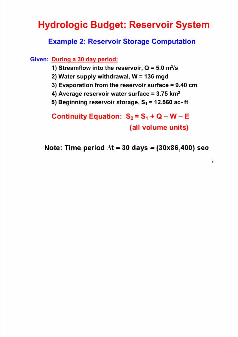
Hydrologic Budget: Reservoir System
Example 2: Reservoir Storage Computation
Given: During a 30 day period:
1) Streamflow into the reservoir, Q = 5.0 m3 /s
2) Water supply withdrawal, W = 136 mgd
3) Evaporation from the reservoir surface = 9.40 cm
4) Average reservoir water surface = 3.75 km
2
, ,
Continuity Equation: S2 = S1 + Q – W – E
a vo ume un s
= =
7
,

7/21/2019 Pe Civil Hydrology Fall 2011
http://slidepdf.com/reader/full/pe-civil-hydrology-fall-2011 8/109
Hydrologic Budget: Reservoir SystemExample 2: Reservoir Storage Computation (Cont.)
Compute: The month-end reservoir storage, S2 in m3 and ac- ft.
= - Note: Streamflow Q is converted
2) Q = (5.0 m3 /s)(30 days)(86,400s/day)= 12,960,000m3 (35.314 ft3 /m3)(2.296x10-5 ac-ft/ft3) = 10,508 ac-ft
to volume for the 30 day period
3) W = (136x106 gal/day)(0.003785 m3 /gal)(30 days)
= 15,442,800 m3 (35.314 ft3 /m3)(2.296x10-5 ac-ft/ft3) = 12,521 ac-ft
4 E = 3.75km2 1x10⁶ m2 /km2 9.4 cm 0.01 m/cm
= 352,500 m3 (35.314 ft3 /m3)(2.296x10-5 ac-ft/ft3) = 286 ac-ft
5) S2 = S1 + Q – W – E (for ∆t = 30 days) ac-ft
= (12,560 + 10,508) – (12,521 + 286)
S2 = 10,261 ac-ft (loss of storage) (Note: S1 = 12,560 ac-ft)
8Note: Change in storage, ΔS = S2 – S1 = (10,261-12,560) = - 2299 ac- ft (loss)

7/21/2019 Pe Civil Hydrology Fall 2011
http://slidepdf.com/reader/full/pe-civil-hydrology-fall-2011 9/109
Problem 1: Reservoir Storage Computation
Given:• Reservoir located at the outlet of a 150 sq. mile watershed
• Mean annual rainfall, P = 38 inches (use as inflow into reservoir)
• Mean annual watershed runoff (flow into reservoir), Q = 13 inches
• ,
• Mean daily withdrawal from reservoir (draft), D = 100 MGD• Mean reservoir surface area, AS = 4000 acres
. . . - , . . - . .1.0 cfs = 1.9835 ac-ft/day))
Using a time frame, Δt = 1 year (365 days) determine:
1. Volume of water evaporated from lake in acre-ft/yr:
a) 16,333 b) 24,586 c) 392,000 d) 55,600
2. Watershed runoff or inflow into reservoir in acre-ft/yr:
9
, , , , ,
Note: Watershed area not adjusted for reservoir area of 4000 acres
7/21/2019 Pe Civil Hydrology Fall 2011
http://slidepdf.com/reader/full/pe-civil-hydrology-fall-2011 10/109
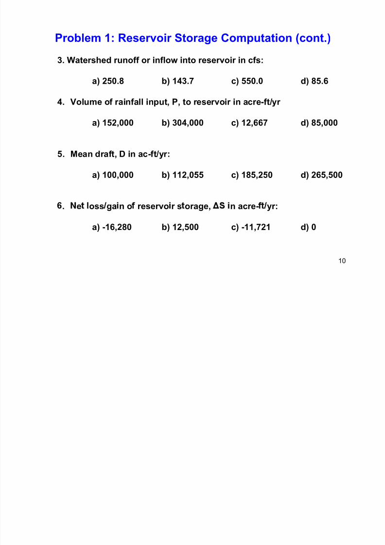
Problem 1: Reservoir Storage Computation (cont.)
3. Watershed runoff or inflow into reservoir in cfs:
a) 250.8 b) 143.7 c) 550.0 d) 85.6
4. Volume of rainfall input, P, to reservoir in acre-ft/yr
a) 152,000 b) 304,000 c) 12,667 d) 85,000
5. Mean draft, D in ac-ft/yr:
a) 100,000 b) 112,055 c) 185,250 d) 265,500
. e oss ga n o reservo r s orage, n acre- yr:
a) -16,280 b) 12,500 c) -11,721 d) 0
10
7/21/2019 Pe Civil Hydrology Fall 2011
http://slidepdf.com/reader/full/pe-civil-hydrology-fall-2011 11/109
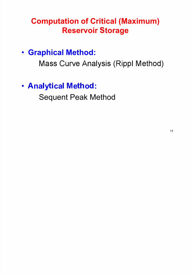
Computation of Critical (Maximum)
Reservoir torage
• Graphical Method:
• na y ca e o :
Sequent Peak Method
11
7/21/2019 Pe Civil Hydrology Fall 2011
http://slidepdf.com/reader/full/pe-civil-hydrology-fall-2011 12/109
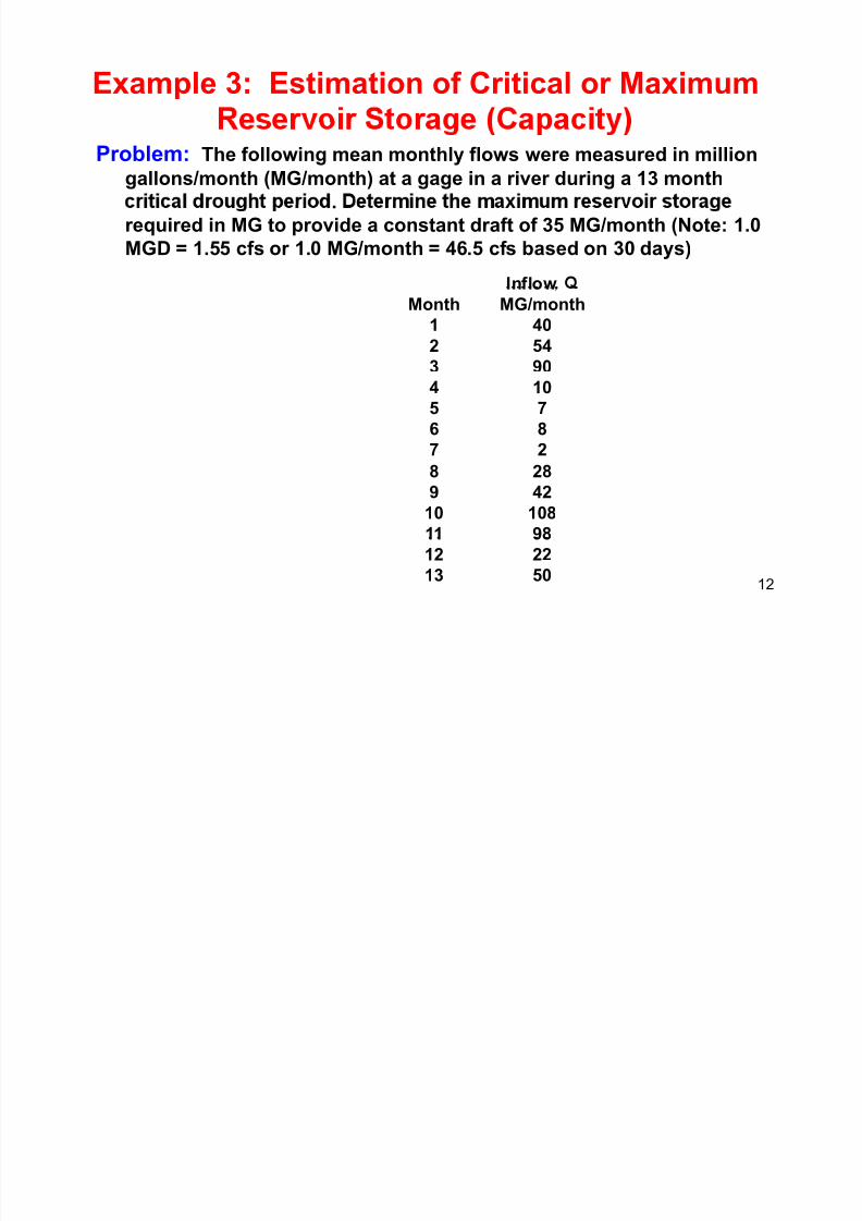
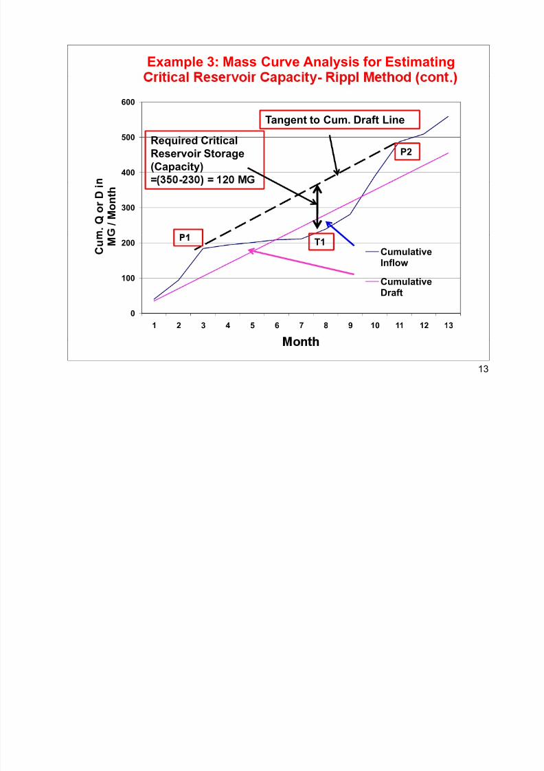
Example 3: Estimation of Critical or Maximum
Problem: The following mean monthly flows were measured in million
gallons/month (MG/month) at a gage in a river during a 13 month
.
required in MG to provide a constant draft of 35 MG/month (Note: 1.0MGD = 1.55 cfs or 1.0 MG/month = 46.5 cfs based on 30 days)
Inflow
Month MG/month
1 40
2 543 90
4 10
5 7
6 8
7 2
8 289 42
10 108
11 98
12
12 22
13 50
7/21/2019 Pe Civil Hydrology Fall 2011
http://slidepdf.com/reader/full/pe-civil-hydrology-fall-2011 13/109
Example 3: Mass Curve Analysis for Estimating
600
- .
Tangent to Cum. Draft Line
400
500 Required Critical
Reservoir Storage
(Capacity)
= - =
P2
300
. Q
o r D i
/
M o n t h
100
200 C u M
CumulativeInflow
Cumulative
T1
0
1 2 3 4 5 6 7 8 9 10 11 12 13
Draft
13
7/21/2019 Pe Civil Hydrology Fall 2011
http://slidepdf.com/reader/full/pe-civil-hydrology-fall-2011 14/109
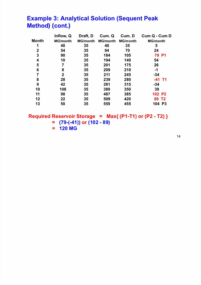
Example 3: Analytical Solution (Sequent Peak
Method cont.Inflow, Q Draft, D Cum. Q Cum. D Cum Q - Cum D
Month MG/month MG/month MG/month MG/month MG/month
1 40 35 40 35 5
2 54 35 94 70 24
3 90 35 184 105 79 P14 10 35 194 140 54
5 7 35 201 175 26
6 8 35 209 210 -1
7 2 35 211 245 -34
8 28 35 239 280 -41 T1
9 42 35 281 315 -34
10 108 35 389 350 39
11 98 35 487 385 102 P2
12 22 35 509 420 89 T2
13 50 35 559 455 104 P3
Required Reservoir Storage = Max{ (P1-T1) or (P2 - T2) }
= (79-(-41)) or (102 - 89)
14
= 120 MG
7/21/2019 Pe Civil Hydrology Fall 2011
http://slidepdf.com/reader/full/pe-civil-hydrology-fall-2011 15/109
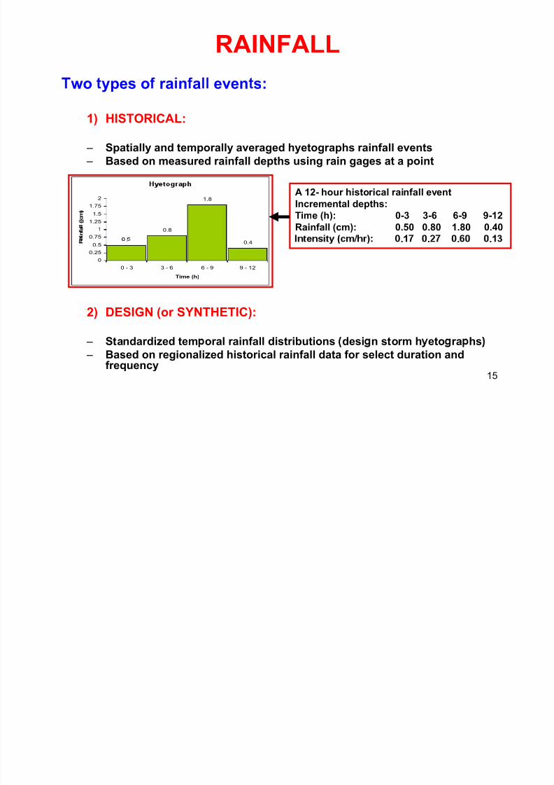
RAINFALL
wo ypes o ra n a even s:
1) HISTORICAL:
– Spatially and temporally averaged hyetographs rainfall events – Based on measured rainfall depths using rain gages at a point
0.8
1.8
0.75
1
1.25
1.5
1.75
2
i n f a l l ( ( c m )
A 12- hour historical rainfall event
Incremental depths:
Time (h): 0-3 3-6 6-9 9-12
Rainfall (cm): 0.50 0.80 1.80 0.40.
0.4
0
0.25
0.5
0 - 3 3 - 6 6 - 9 9 - 12
Time (h)
R . . . .
2) DESIGN (or SYNTHETIC):
– Standardized tem oral rainfall distributions desi n storm h eto ra hs
15
– Based on regionalized historical rainfall data for select duration andfrequency
7/21/2019 Pe Civil Hydrology Fall 2011
http://slidepdf.com/reader/full/pe-civil-hydrology-fall-2011 16/109
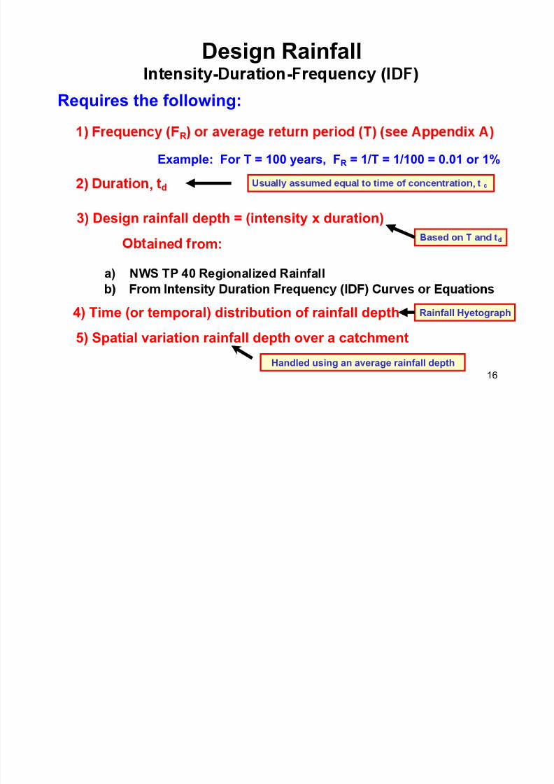
Design Rainfall
- -Requires the following:
R
Example: For T = 100 years, FR = 1/T = 1/100 = 0.01 or 1%
,
3) Design rainfall depth = (intensity x duration)
,
a ne rom:
a) NWS TP 40 Regionalized Rainfall
4) Time (or temporal) distribution of rainfall depth
5) Spatial variation rainfall depth over a catchment
Rainfall Hyetograph
16
Handled using an average rainfall depth
7/21/2019 Pe Civil Hydrology Fall 2011
http://slidepdf.com/reader/full/pe-civil-hydrology-fall-2011 17/109
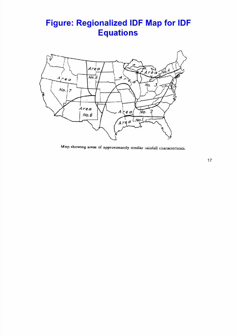
Figure: Regionalized IDF Map for IDF
17
7/21/2019 Pe Civil Hydrology Fall 2011
http://slidepdf.com/reader/full/pe-civil-hydrology-fall-2011 18/109
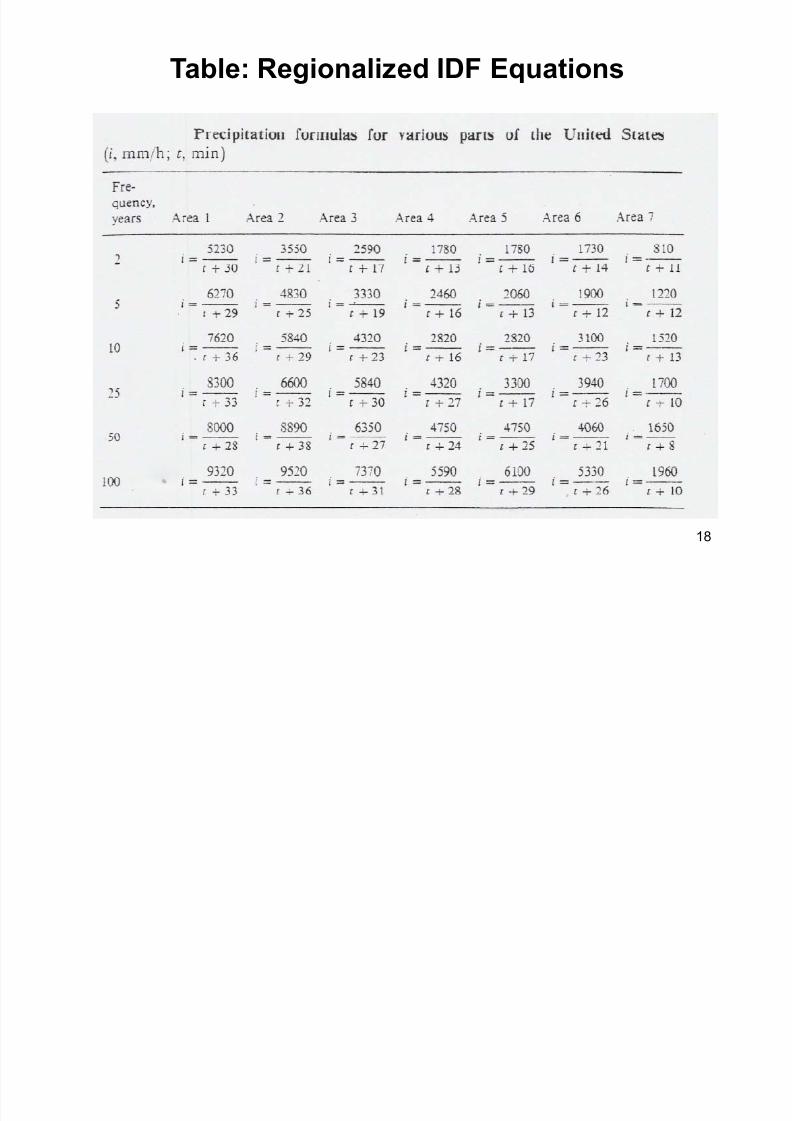
Table: Regionalized IDF Equations
18
7/21/2019 Pe Civil Hydrology Fall 2011
http://slidepdf.com/reader/full/pe-civil-hydrology-fall-2011 19/109
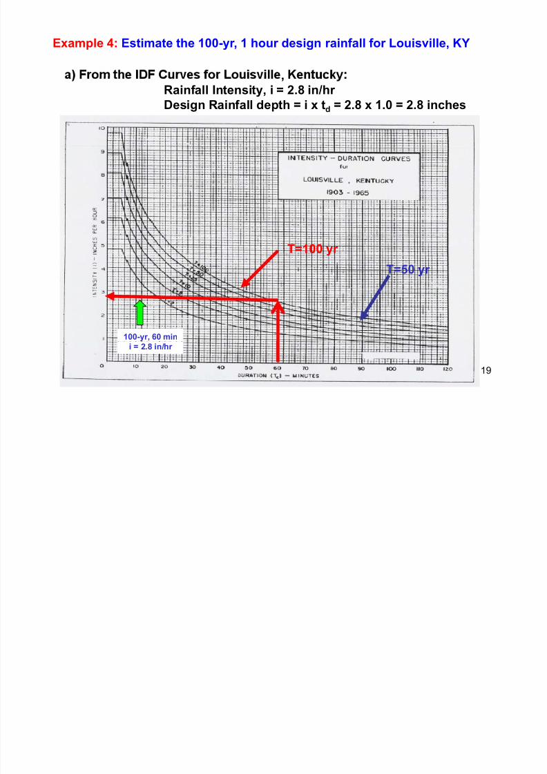
Example 4: Estimate the 100-yr, 1 hour design rainfall for Louisville, KY
,Rainfall Intensity, i = 2.8 in/hr
Design Rainfall depth = i x td = 2.8 x 1.0 = 2.8 inches
T=100 yr
T=50 yr
100-yr, 60 min
19
i = 2.8 in/hr
7/21/2019 Pe Civil Hydrology Fall 2011
http://slidepdf.com/reader/full/pe-civil-hydrology-fall-2011 20/109
Example 4: Estimate the 100-yr, 1 hour design rainfall for
Louisville, KY (cont.)
b) From the IDF Map and Table (Slides 17 and 18) Louisville is in
.
Regional IDF equation for T =100 yr :i (mm/hr) = { 7370/(t+31) } where t = td in minutes
i = 7370/(60+31)
= 80.989 mm/hr
= 3.2 in/hr
Rainfall Depth = 3.2 in From Louisville IDF Curve P = 2.80 in
(see previous slide)
• Note the difference between using a locally developedIDF curve versus using a regional equation
20
7/21/2019 Pe Civil Hydrology Fall 2011
http://slidepdf.com/reader/full/pe-civil-hydrology-fall-2011 21/109
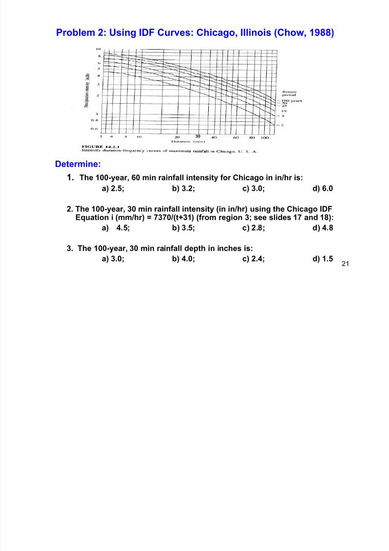
Problem 2: Using IDF Curves: Chicago, Illinois (Chow, 1988)
Determine:
30
1. The 100-year, 60 min rainfall intensity for Chicago in in/hr is:
a) 2.5; b) 3.2; c) 3.0; d) 6.0
2. The 100-year, 30 min rainfall intensity (in in/hr) using the Chicago IDFEquation i (mm/hr) = 7370/(t+31) (from region 3; see slides 17 and 18):
a) 4.5; b) 3.5; c) 2.8; d) 4.8
21
3. The 100-year, 30 min rainfall depth in inches is:
a) 3.0; b) 4.0; c) 2.4; d) 1.5
7/21/2019 Pe Civil Hydrology Fall 2011
http://slidepdf.com/reader/full/pe-civil-hydrology-fall-2011 22/109
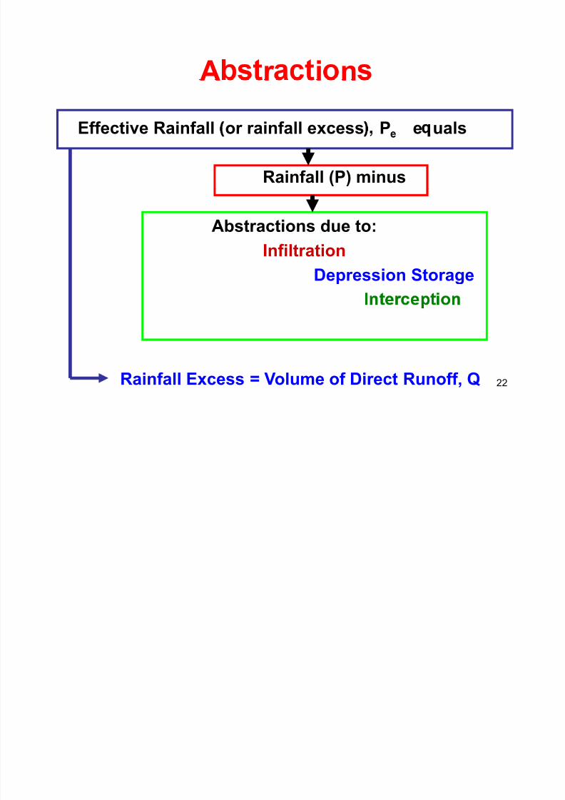
A r i nEffective Rainfall or rainfall excess P e uals
Rainfall (P) minus
Abstractions due to:Infiltration
Depression Storage
22Rainfall Excess = Volume of Direct Runoff, Q
7/21/2019 Pe Civil Hydrology Fall 2011
http://slidepdf.com/reader/full/pe-civil-hydrology-fall-2011 23/109
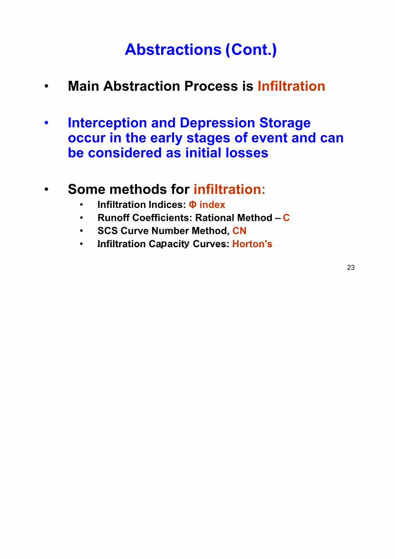
Abstractions Cont.
• Main Abstraction Process is Infiltration
• Interception and Depression Storageoccur in the early stages of event and canbe considered as initial losses
• Some methods for infiltration:• Infiltration Indices: Φ index
• Runoff Coefficients: Rational Method – C• SCS Curve Number Method, CN
• Infiltration Ca acit Curves: Horton's
23
7/21/2019 Pe Civil Hydrology Fall 2011
http://slidepdf.com/reader/full/pe-civil-hydrology-fall-2011 24/109
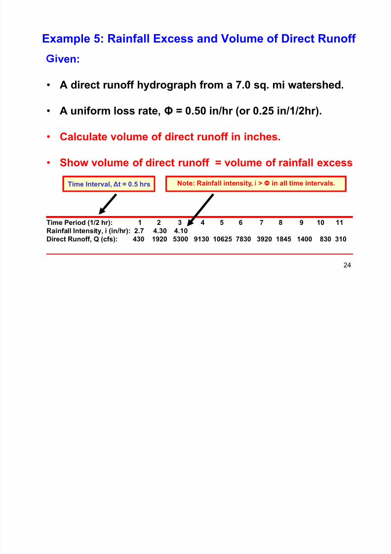
Example 5: Rainfall Excess and Volume of Direct Runoff
ven:
• A direct runoff hydrograph from a 7.0 sq. mi watershed.
• A uniform loss rate, Φ = 0.50 in/hr (or 0.25 in/1/2hr).
• Calculate volume of direct runoff in inches.
• Show volume of direct runoff = volume of rainfall excess
Time Interval, Δt = 0.5 hrs Note: Rainfall intensity, i > Φ in all time intervals.
________________________________________ Time Period (1/2 hr): 1 2 3 4 5 6 7 8 9 10 11
Rainfall Intensity, i (in/hr): 2.7 4.30 4.10
Direct Runoff, Q (cfs): 430 1920 5300 9130 10625 7830 3920 1845 1400 830 310
24
________________________________________________________
7/21/2019 Pe Civil Hydrology Fall 2011
http://slidepdf.com/reader/full/pe-civil-hydrology-fall-2011 25/109
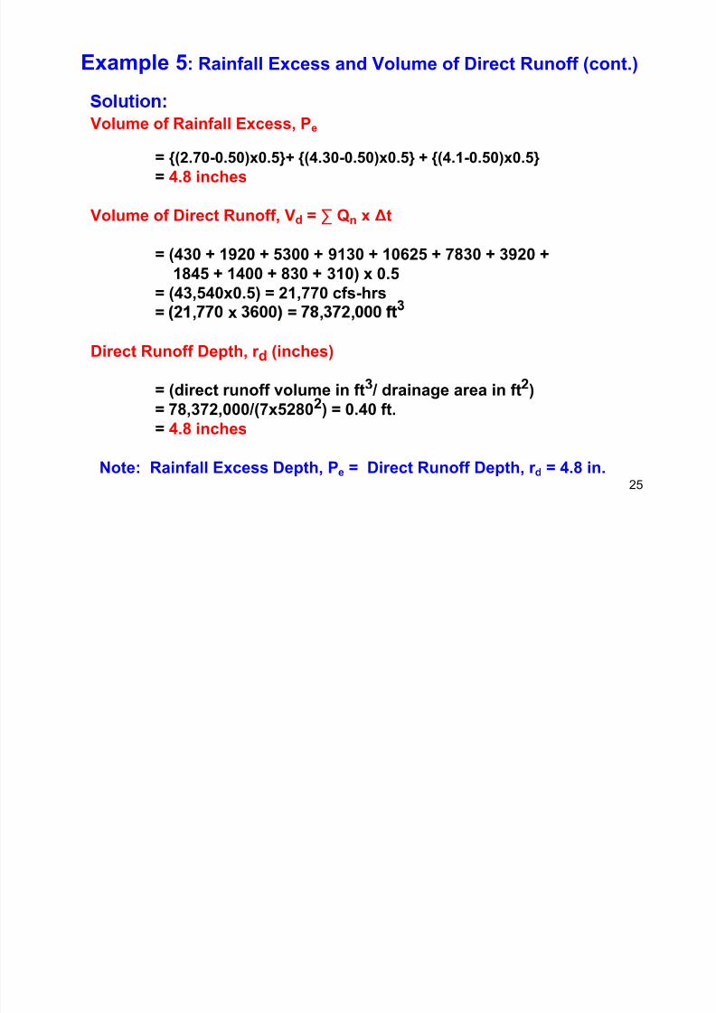
Example 5: Rainfall Excess and Volume of Direct Runoff (cont.)
Volume of Rainfall Excess, Pe
= {(2.70-0.50)x0.5}+ {(4.30-0.50)x0.5} + {(4.1-0.50)x0.5}
= 4.8 inches
Volume of Direct Runoff, Vd = ∑ Qn x Δt
= (430 + 1920 + 5300 + 9130 + 10625 + 7830 + 3920 +
1845 + 1400 + 830 + 310) x 0.5
= (43,540x0.5) = 21,770 cfs-hrs= , x = , ,
Direct Runoff Depth, r d (inches)
= (direct runoff volume in ft3 / drainage area in ft2)= 78,372,000/(7x52802) = 0.40 ft.
= 4.8 inches
25
Note: Rainfall Excess Depth, Pe = Direct Runoff Depth, r d = 4.8 in.
7/21/2019 Pe Civil Hydrology Fall 2011
http://slidepdf.com/reader/full/pe-civil-hydrology-fall-2011 26/109
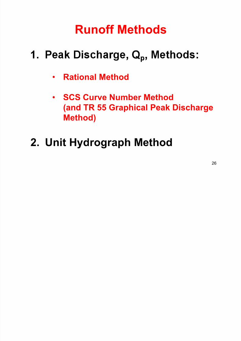
Runoff Methods
• Rational Method
• SCS Curve Number Method(and TR 55 Graphical Peak Discharge
Method)
2. Unit Hydrograph Method
26
7/21/2019 Pe Civil Hydrology Fall 2011
http://slidepdf.com/reader/full/pe-civil-hydrology-fall-2011 27/109
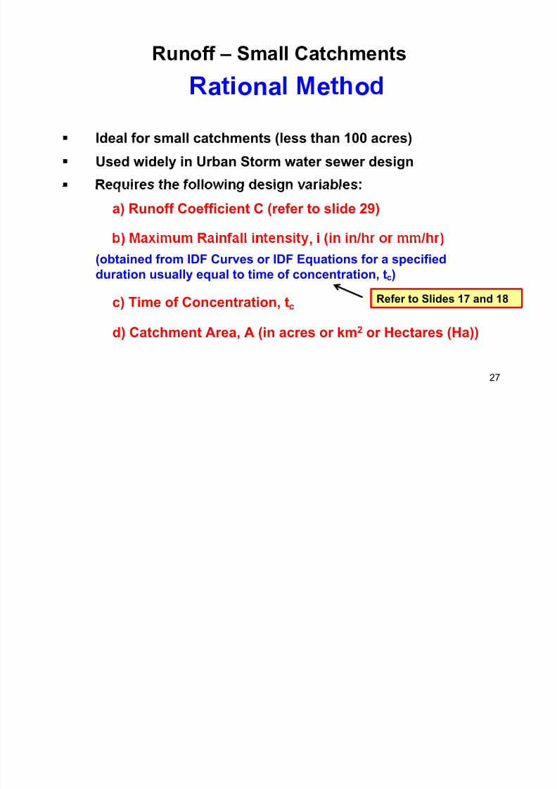
Runoff – Small Catchments
a ona e o
Ideal for small catchments (less than 100 acres)
Used widely in Urban Storm water sewer design
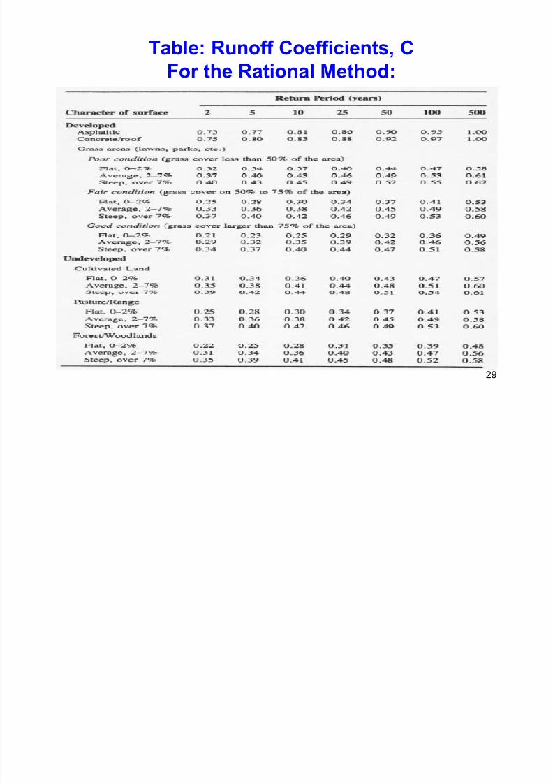
a) Runoff Coefficient C (refer to slide 29)
,
(obtained from IDF Curves or IDF Equations for a specified
duration usually equal to time of concentration, tc)
c) Time of Concentration, tc
d) Catchment Area, A (in acres or km2 or Hectares (Ha))
Refer to Slides 17 and 18
27
7/21/2019 Pe Civil Hydrology Fall 2011
http://slidepdf.com/reader/full/pe-civil-hydrology-fall-2011 28/109
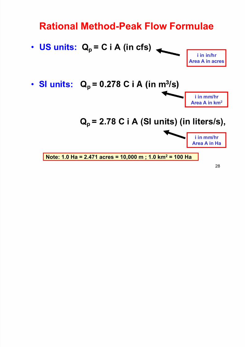
Rational Method-Peak Flow Formulae
• US units: Qp = C i A (in cfs)i in in/hr
Area A in acres
• un s: p = . n m s
i in mm/hr
Area A in km2
Qp = 2.78 C i A (SI units) (in liters/s),
i in mm/hr
Area A in Ha
28
Note: 1.0 Ha = 2.471 acres = 10,000 m ; 1.0 km2 = 100 Ha
7/21/2019 Pe Civil Hydrology Fall 2011
http://slidepdf.com/reader/full/pe-civil-hydrology-fall-2011 29/109
Table: Runoff Coefficients, C
For the Rational Method:
29

7/21/2019 Pe Civil Hydrology Fall 2011
http://slidepdf.com/reader/full/pe-civil-hydrology-fall-2011 30/109
Time of Concentration, tc
Definition:
tC = ∑travel times from thehydraulically remotest point in a
= (Overland flow time)
+ (Channel or Pipe flow) timeRefer to Appendix A for Methods for
Computing Time of Concentrationt3t4
Example: tc at this outlet
30
= max (t1 + t2) or t3 or t4
7/21/2019 Pe Civil Hydrology Fall 2011
http://slidepdf.com/reader/full/pe-civil-hydrology-fall-2011 31/109
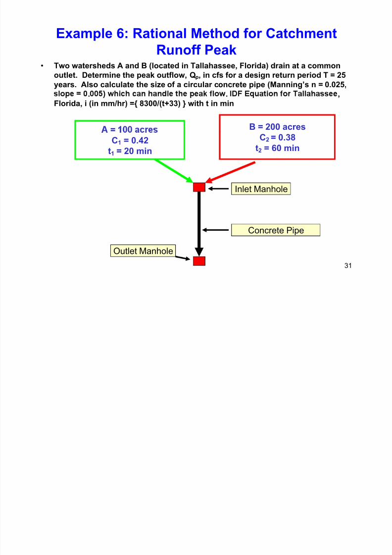
Example 6: Rational Method for Catchment
Runoff Peak• Two watersheds A and B (located in Tallahassee, Florida) drain at a common
outlet. Determine the peak outflow, Qp, in cfs for a design return period T = 25
years. Also calculate the size of a circular concrete pipe (Manning’s n = 0.025,
. . ,
Florida, i (in mm/hr) ={ 8300/(t+33) } with t in min
= B = 200 acres
C1 = 0.42
t1 = 20 min
C2 = 0.38
t2 = 60 min
Inlet Manhole
Concrete Pipe
31
Outlet Manhole

7/21/2019 Pe Civil Hydrology Fall 2011
http://slidepdf.com/reader/full/pe-civil-hydrology-fall-2011 32/109
Example 6: Rational Method for Catchment Runoff Peak (cont.)
• Composite Cc = (C1A1 + C2A2)/(A1+A2)
• = (0.42x100 + 0.38x200)/(100+200) = 0.39Note for multiple areas:
• Time of Concentration, tc = max ( t1, t2) = max (20, 60) = 60 min
Qp = Cc i AT = (∑Ci i /∑Ai) AT = i ∑CiAi
where total area, A T = ∑A i
• 25-year Rainfall intensity I for tc = 60 min = 3.5 in/hr
Tallahassee, FL, IDF Eq. Area 1 (slide 18)
i (mm/hr) ={8300/(t+33)} with t in min
• Peak Flow Qp = CciA = 0.39x3.5x300 = 409.5 cfs
Rational Method Formula (US units)
• Pipe diameter, D = { 2.16x409.5x0.020/ (0.005)0.5 }3/8 = 7.93 feet
rom ann ng s n s
D = (2.16xQpn/√So)3/8
32
.

7/21/2019 Pe Civil Hydrology Fall 2011
http://slidepdf.com/reader/full/pe-civil-hydrology-fall-2011 33/109
Problem 3: Application of Rational Method in Storm Sewer
Design
Given:
IDF Equation for the area is:
i (in/hr) = 120T 0.175
d
where T = Return Period in yearstd = Storm duration = time of
concentration, tc in minutes
Pipe EB
Elv. E = 498.43 ft; Elv. B = 495.55
Length of pipe EB = 450 ft
33
Determine Peak Flow from Sub-area Area III and
Pipe size EB Using Rational Method
7/21/2019 Pe Civil Hydrology Fall 2011
http://slidepdf.com/reader/full/pe-civil-hydrology-fall-2011 34/109
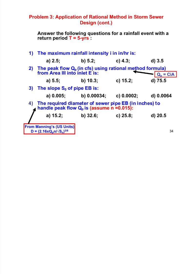
Problem 3: Application of Rational Method in Storm Sewer
Design (cont.)
Answer the following questions for a rainfall event with areturn period T = 5-yrs :
1) The maximum rainfall intensity i in in/hr is:a) 2.5; b) 5.2; c) 4.3; d) 3.5
2) The peak flow Qp (in cfs) using rational method formula)from Area III into inlet E is:
a) 5.5; b) 10.3; c) 15.2; d) 75.5
Qp = CiA
3) The slope S0 of pipe EB is:
a) 0.005; b) 0.00034; c) 0.0002; d) 0.0064
e requ re ame er o sewer p pe n nc es ohandle peak flow Qp is (assume n =0.015):
a) 15.2; b) 32.6; c) 25.8; d) 20.5
34
From Manning’s (US Units)
D = (2.16xQpn/√So)3/8
7/21/2019 Pe Civil Hydrology Fall 2011
http://slidepdf.com/reader/full/pe-civil-hydrology-fall-2011 35/109
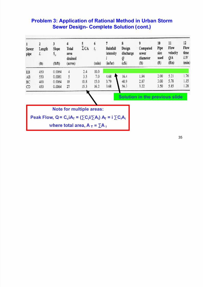
Problem 3: Application of Rational Method in Urban Storm
Sewer Desi n- Com lete Solution cont.
Solution in the previous slide
Note for multiple areas:
Peak Flow, Q = CciAT = (∑Cii/∑Ai) AT = i ∑CiAi
=
35
7/21/2019 Pe Civil Hydrology Fall 2011
http://slidepdf.com/reader/full/pe-civil-hydrology-fall-2011 36/109
Runoff - Midsize Catchments:
SCS TR55 Method
36
7/21/2019 Pe Civil Hydrology Fall 2011
http://slidepdf.com/reader/full/pe-civil-hydrology-fall-2011 37/109
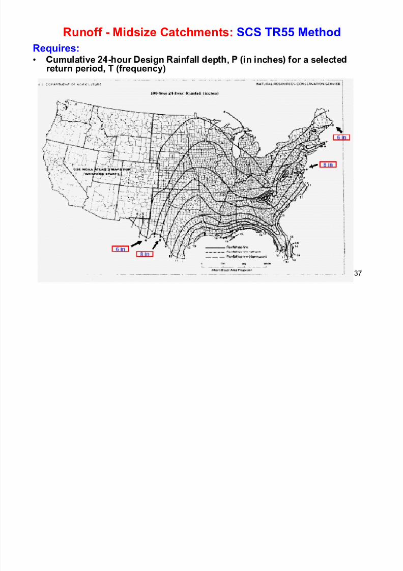
Runoff - Midsize Catchments: SCS TR55 Method
Requires:
• umu a ve - our es gn a n a ep , n nc es or a se ec ereturn period, T (frequency)
37
Runoff Midsize Catchments: SCS TR55 Method (cont )
7/21/2019 Pe Civil Hydrology Fall 2011
http://slidepdf.com/reader/full/pe-civil-hydrology-fall-2011 38/109
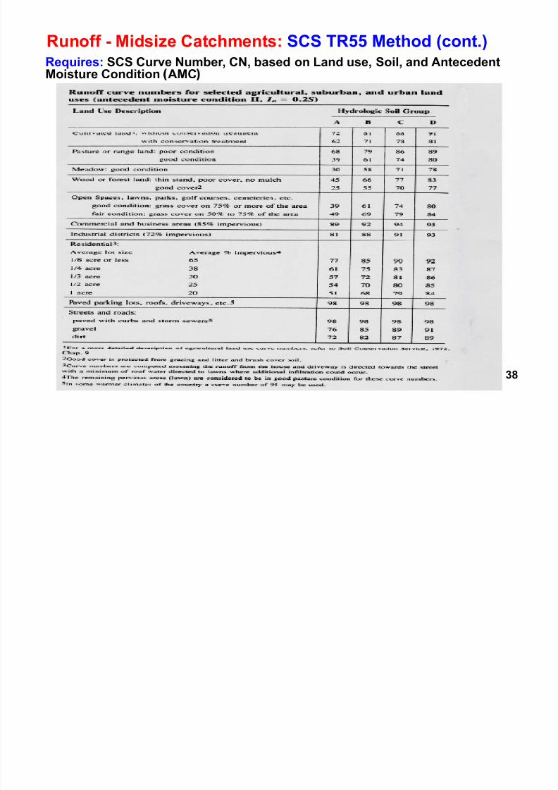
Runoff - Midsize Catchments: SCS TR55 Method (cont.)Requires: SCS Curve Number, CN, based on Land use, Soil, and AntecedentMoisture Condition AMC
38
7/21/2019 Pe Civil Hydrology Fall 2011
http://slidepdf.com/reader/full/pe-civil-hydrology-fall-2011 39/109
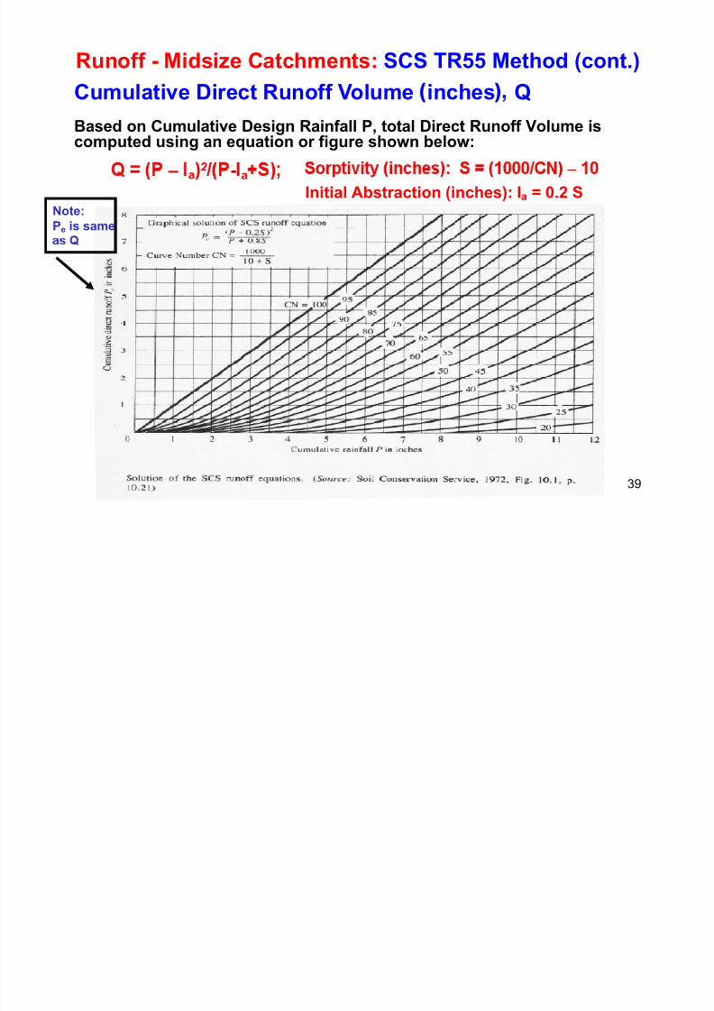
Runoff - Midsize Catchments: SCS TR55 Method (cont.)
Cumulative Direct Runoff Volume inches Q
Based on Cumulative Design Rainfall P, total Direct Runoff Volume iscomputed using an equation or figure shown below:
2 – – a - a
Initial Abstraction (inches): Ia
= 0.2 SNote:
Pe is same
39
7/21/2019 Pe Civil Hydrology Fall 2011
http://slidepdf.com/reader/full/pe-civil-hydrology-fall-2011 40/109
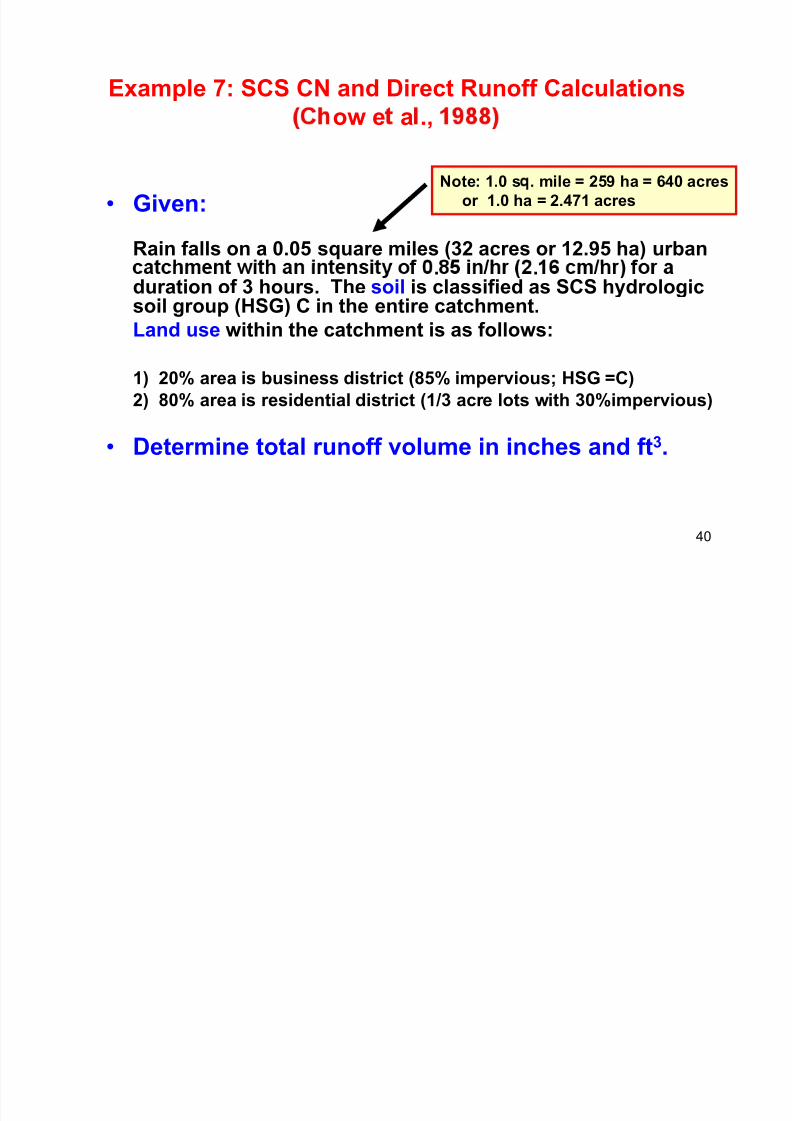
Example 7: SCS CN and Direct Runoff Calculations
ow e a .,
Note: 1.0 s . mile = 259 ha = 640 acres
• Given:
Rain falls on a 0.05 square miles (32 acres or 12.95 ha) urban
or 1.0 ha = 2.471 acres
. .duration of 3 hours. The soil is classified as SCS hydrologicsoil group (HSG) C in the entire catchment.
Land use within the catchment is as follows:
1) 20% area is business district (85% impervious; HSG =C)
2) 80% area is residential district (1/3 acre lots with 30%impervious)
• Determine total runoff volume in inches and ft3.
40
E l 7 SCS CN d Di t R ff C l l ti
7/21/2019 Pe Civil Hydrology Fall 2011
http://slidepdf.com/reader/full/pe-civil-hydrology-fall-2011 41/109
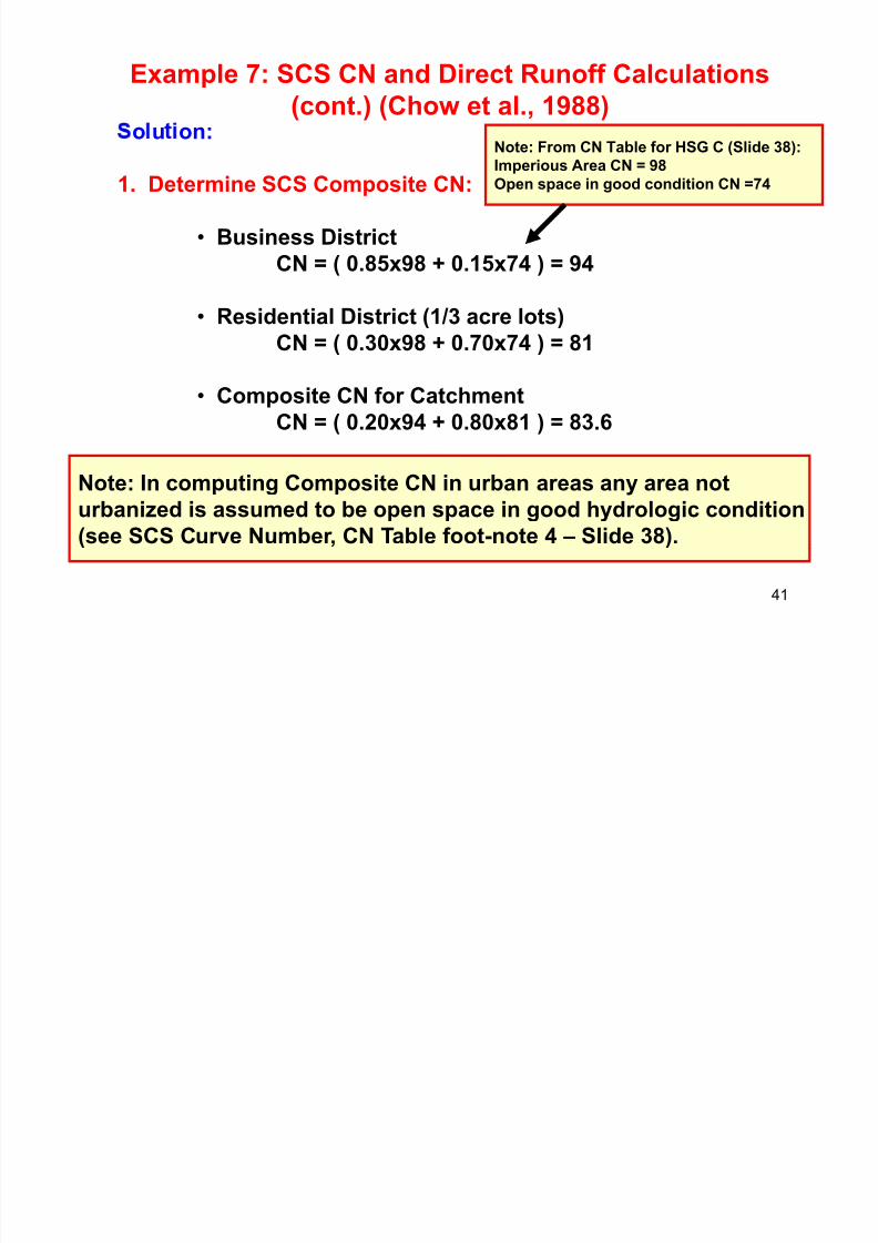
Example 7: SCS CN and Direct Runoff Calculations
(cont.) (Chow et al., 1988)
o u on:
1. Determine SCS Composite CN:
Note: From CN Table for HSG C (Slide 38):
Imperious Area CN = 98
Open space in good condition CN =74
• Business DistrictCN = ( 0.85x98 + 0.15x74 ) = 94
• Residential District (1/3 acre lots)
CN = ( 0.30x98 + 0.70x74 ) = 81
• Composite CN for Catchment
CN = ( 0.20x94 + 0.80x81 ) = 83.6
Note: In computing Composite CN in urban areas any area noturbanized is assumed to be open space in good hydrologic condition
(see SCS Curve Number, CN Table foot-note 4 – Slide 38).
41
E l 7 SCS CN d Di t R ff C l l ti
7/21/2019 Pe Civil Hydrology Fall 2011
http://slidepdf.com/reader/full/pe-civil-hydrology-fall-2011 42/109
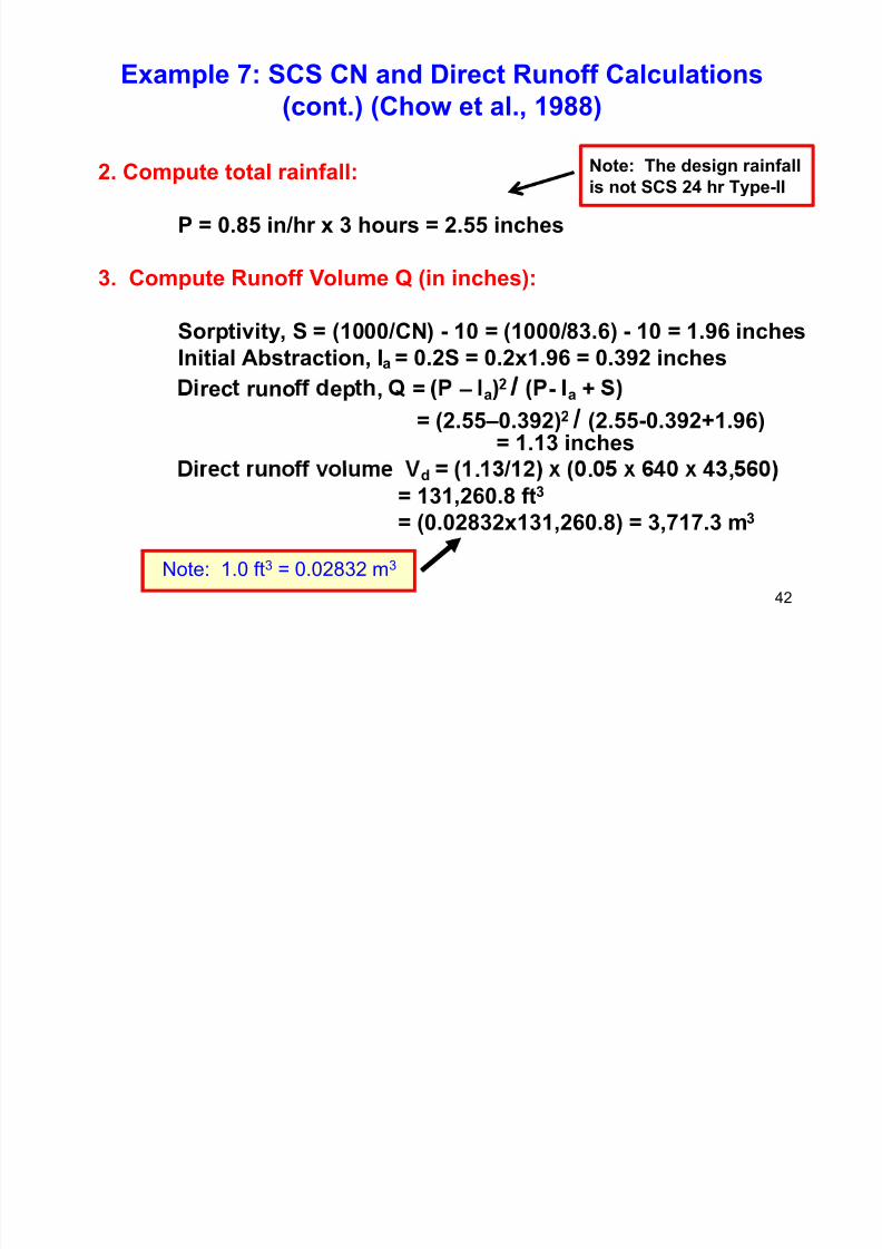
Example 7: SCS CN and Direct Runoff Calculations
(cont.) (Chow et al., 1988)
2. Compute total rainfall: Note: The design rainfall
is not SCS 24 hr Type-II
P = 0.85 in/hr x 3 hours = 2.55 inches
3. Compute Runoff Volume Q (in inches):
Sorptivity, S = (1000/CN) - 10 = (1000/83.6) - 10 = 1.96 inches
Initial Abstraction, Ia = 0.2S = 0.2x1.96 = 0.392 inchesrec runo ep , = – a
- a +
= (2.55–0.392)2 / (2.55-0.392+1.96)= 1.13 inches
d . . ,
= 131,260.8 ft3
= (0.02832x131,260.8) = 3,717.3 m3
42
Note: 1.0 ft3 = 0.02832 m3
7/21/2019 Pe Civil Hydrology Fall 2011
http://slidepdf.com/reader/full/pe-civil-hydrology-fall-2011 43/109
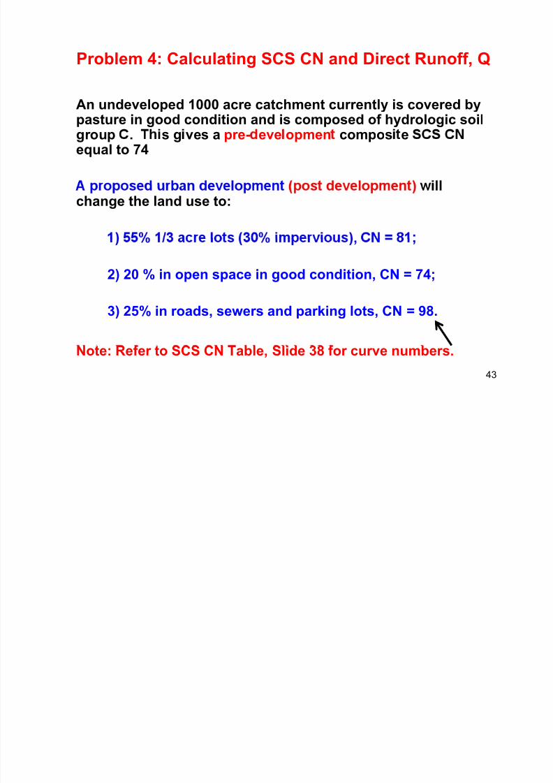
Problem 4: Calculating SCS CN and Direct Runoff, Q
An undeveloped 1000 acre catchment currently is covered bypasture in good condition and is composed of hydrologic soilgroup . s g ves a pre- eve opmen compos e
equal to 74
change the land use to:
,
2) 20 % in open space in good condition, CN = 74;
3) 25% in roads, sewers and parking lots, CN = 98.
43
Note: Refer to SCS CN Table, Slide 38 for curve numbers.
7/21/2019 Pe Civil Hydrology Fall 2011
http://slidepdf.com/reader/full/pe-civil-hydrology-fall-2011 44/109
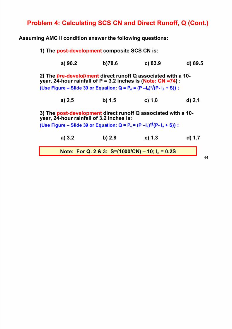
Problem 4: Calculating SCS CN and Direct Runoff, Q (Cont.)
Assuming AMC II condition answer the following questions:
1) The post-development composite SCS CN is:
a) 90.2 b)78.6 c) 83.9 d) 89.5
2 The re-develo ment direct runoff Q associated with a 10-year, 24-hour rainfall of P = 3.2 inches is (Note: CN =74) :
(Use Figure – Slide 39 or Equation: Q = Pe = (P –Ia)2 /(P- Ia + S)) :
. . . .
3) The post-development direct runoff Q associated with a 10-year, 24-hour rainfall of 3.2 inches is:
(Use Figure – Slide 39 or Equation: Q = Pe = (P –Ia)2 (P- Ia + S)) :
a) 3.2 b) 2.8 c) 1.3 d) 1.7
44
Note: For Q. 2 & 3: S=(1000/CN) – 10; Ia = 0.2S
R ff Mid i C t h t SCS TR55 M th d
7/21/2019 Pe Civil Hydrology Fall 2011
http://slidepdf.com/reader/full/pe-civil-hydrology-fall-2011 45/109
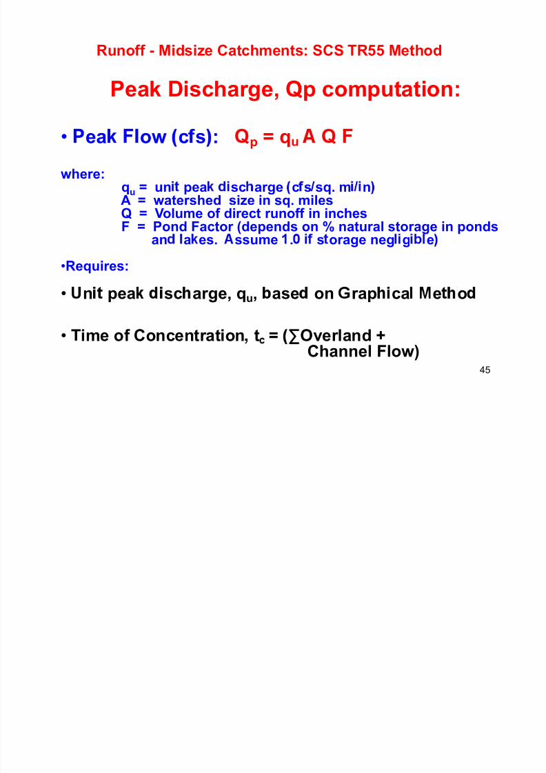
Runoff - Midsize Catchments: SCS TR55 Method
Peak Discharge, Qp computation:
• ea ow c s : p = qu
where:qu = un pea sc arge c s sq. m nA = watershed size in sq. milesQ = Volume of direct runoff in inches
F = Pond Factor (depends on % natural storage in pondsan a es. ssume . s orage neg g e
•Requires:
•n pea sc arge, q
u, ase on rap ca e o
• Time of Concentration t = Overland +
45
Channel Flow)
7/21/2019 Pe Civil Hydrology Fall 2011
http://slidepdf.com/reader/full/pe-civil-hydrology-fall-2011 46/109
Runoff - Midsize Catchments: SCS TR55 Method
Computing Catchment’s Time of Concentration
u w w
for computing catchment's time of
<
2. Overland Shallow Concentrated Flow
3. Channel or Pipe Flow
46
7/21/2019 Pe Civil Hydrology Fall 2011
http://slidepdf.com/reader/full/pe-civil-hydrology-fall-2011 47/109
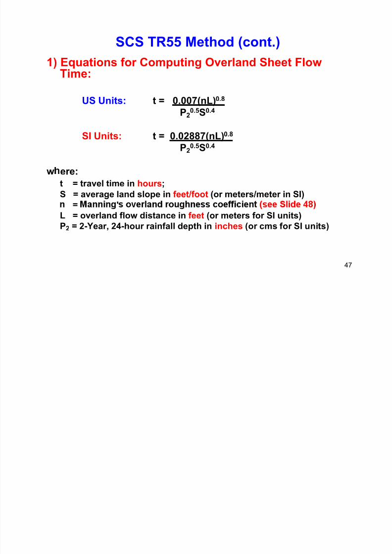
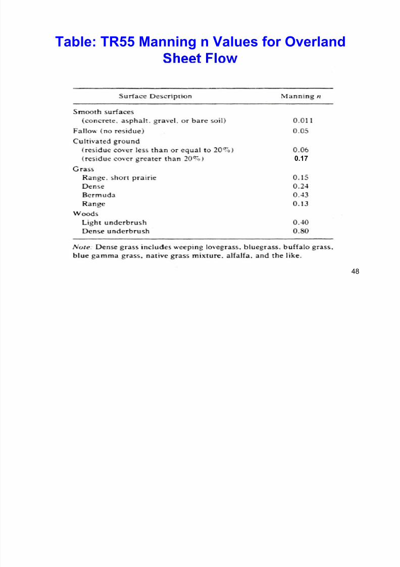
SCS TR55 Method (cont.)
1) Equations for Computing Overland Sheet FlowTime:
US Units: t = 0.007(nL)0.8
P20.5S0.4
SI Units: t = 0.02887(nL)0.8
P20.5S0.4
w ere:
t = travel time in hours;
S = average land slope in feet/foot (or meters/meter in SI)
= '
L = overland flow distance in feet (or meters for SI units)P2 = 2-Year, 24-hour rainfall depth in inches (or cms for SI units)
47
7/21/2019 Pe Civil Hydrology Fall 2011
http://slidepdf.com/reader/full/pe-civil-hydrology-fall-2011 48/109
Table: TR55 Manning n Values for Overland
0.17
48
SCS TR55 Method (cont.)
7/21/2019 Pe Civil Hydrology Fall 2011
http://slidepdf.com/reader/full/pe-civil-hydrology-fall-2011 49/109
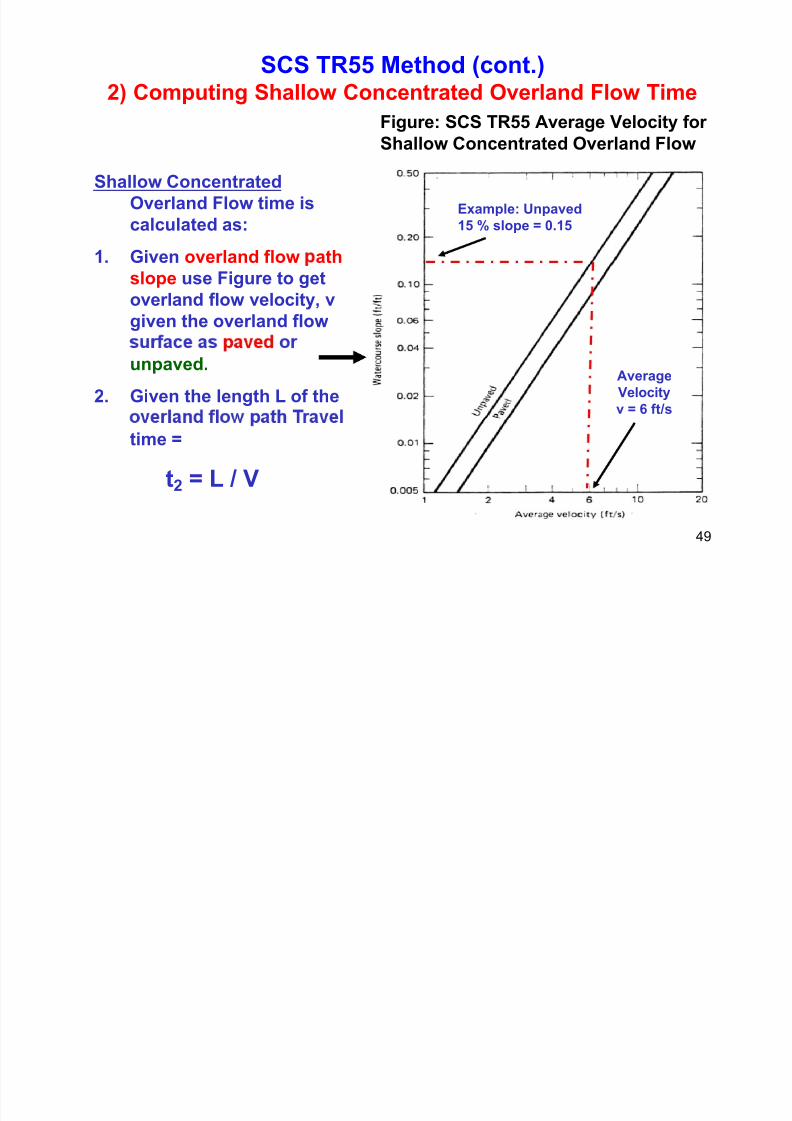
SCS TR55 Method (cont.)2) Computing Shallow Concentrated Overland Flow Time
Shallow Concentrated
Figure: SCS TR55 Average Velocity forShallow Concentrated Overland Flow
Overland Flow time is
calculated as:
1. Given overland flow ath
Example: Unpaved
15 % slope = 0.15
slope use Figure to get
overland flow velocity, v
given the overland flow
unpaved.
2. Given the length L of the
Average
Velocity
v = 6 ft/s
time =
t2 = L / V
49
SCS TR55 M th d ( t )
7/21/2019 Pe Civil Hydrology Fall 2011
http://slidepdf.com/reader/full/pe-civil-hydrology-fall-2011 50/109
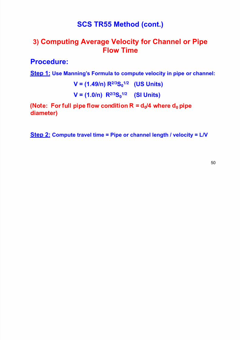
SCS TR55 Method (cont.)
3) Computing Average Velocity for Channel or Pipe
Flow Time
Procedure:
Step 1: Use Manning’s Formula to compute velocity in pipe or channel:
V = (1.49/n) R2/3S01/2 (US Units)
V = (1.0/n) R2/3S01/2 (SI Units)
o e: or u p pe ow con on = 0 w ere 0 p pe
diameter)
Step 2: Compute travel time = Pipe or channel length / velocity = L/V
50
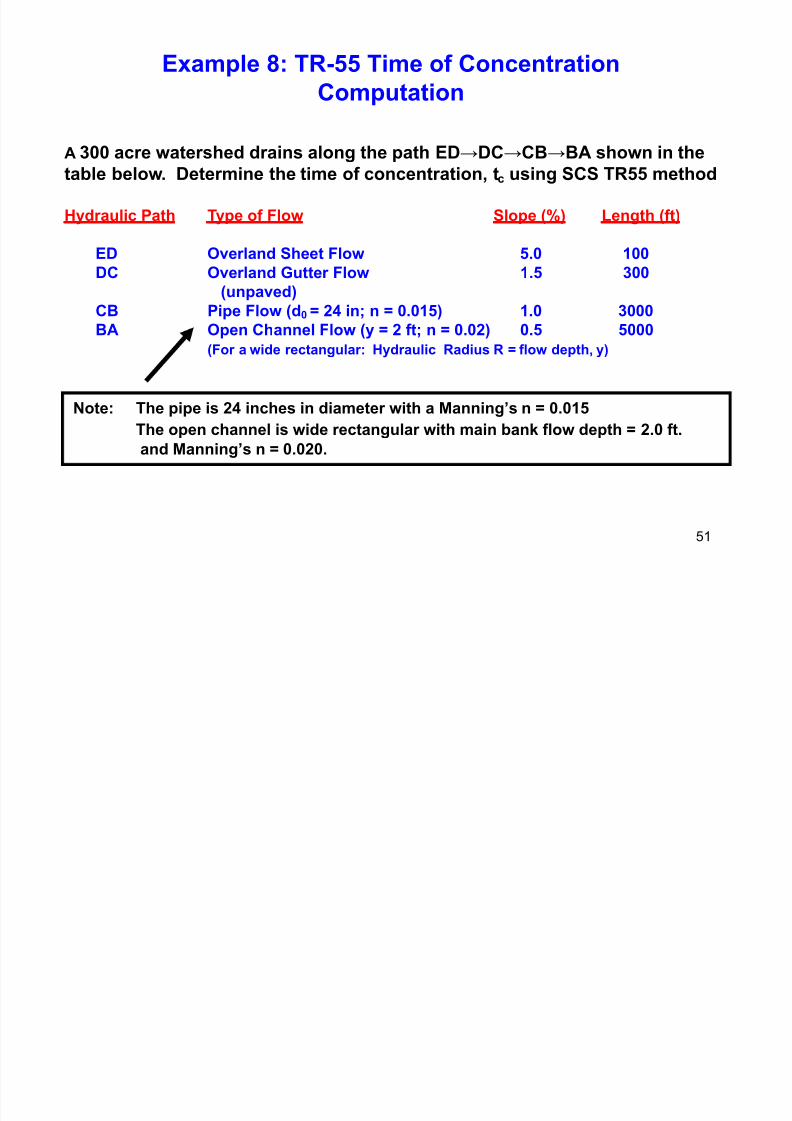
Example 8: TR-55 Time of Concentration
7/21/2019 Pe Civil Hydrology Fall 2011
http://slidepdf.com/reader/full/pe-civil-hydrology-fall-2011 51/109
p
Computation
A 300 acre watershed drains along the path ED→DC→CB→BA shown in the
table below. Determine the time of concentration, tc using SCS TR55 method
Hydraulic Path Type of Flow Slope (%) Length (ft)
ED Overland Sheet Flow 5.0 100
DC Overland Gutter Flow 1.5 300
(unpaved)
CB Pipe Flow (d0 = 24 in; n = 0.015) 1.0 3000
BA Open Channel Flow (y = 2 ft; n = 0.02) 0.5 5000(For a wide rectangular: Hydraulic Radius R = flow depth, y)
Note: The pipe is 24 inches in diameter with a Manning’s n = 0.015
The open channel is wide rectangular with main bank flow depth = 2.0 ft.
and Manning’s n = 0.020.
51
Example 8: TR-55 Time of Concentration Computation (cont.)
7/21/2019 Pe Civil Hydrology Fall 2011
http://slidepdf.com/reader/full/pe-civil-hydrology-fall-2011 52/109
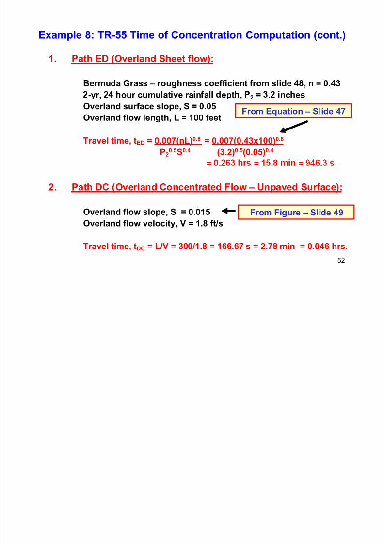
Example 8: TR 55 Time of Concentration Computation (cont.)
1. Path ED (Overland Sheet flow):
Bermuda Grass – roughness coefficient from slide 48, n = 0.43
-yr, our cumu at ve ra n a ept , 2 = . nc es
Overland surface slope, S = 0.05Overland flow length, L = 100 feet
From Equation – Slide 47
Travel time, tED = 0.007(nL)0.8 = 0.007(0.43x100)0.8
P20.5S0.4 (3.2)0.5(0.05)0.4
= = =
2. Path DC (Overland Concentrated Flow – Unpaved Surface):
Overland flow slope, S = 0.015Overland flow velocity, V = 1.8 ft/s
From Figure – Slide 49
52
Travel time, tDC = L/V = 300/1.8 = 166.67 s = 2.78 min = 0.046 hrs.
E l 8 TR 55 Ti f C t ti C t ti ( t )
7/21/2019 Pe Civil Hydrology Fall 2011
http://slidepdf.com/reader/full/pe-civil-hydrology-fall-2011 53/109
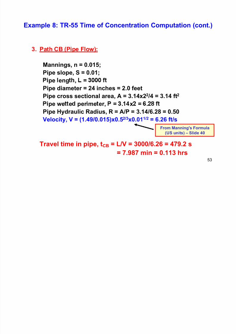
Example 8: TR-55 Time of Concentration Computation (cont.)
3. Path CB (Pipe Flow):
Mannings, n = 0.015;Pipe slope, S = 0.01;
pe eng , =
Pipe diameter = 24 inches = 2.0 feet
Pipe cross sectional area, A = 3.14x22 /4 = 3.14 ft2
pe we e per me er, = . x = .
Pipe Hydraulic Radius, R = A/P = 3.14/6.28 = 0.50
Velocity, V = (1.49/0.015)x0.52/3x0.011/2 = 6.26 ft/s
Travel time in pipe, tCB = L/V = 3000/6.26 = 479.2 s
From Manning's Formula
(US units) – Slide 40
53
= 7.987 min = 0.113 hrs
Example 8: TR-55 Time of Concentration Computation
7/21/2019 Pe Civil Hydrology Fall 2011
http://slidepdf.com/reader/full/pe-civil-hydrology-fall-2011 54/109
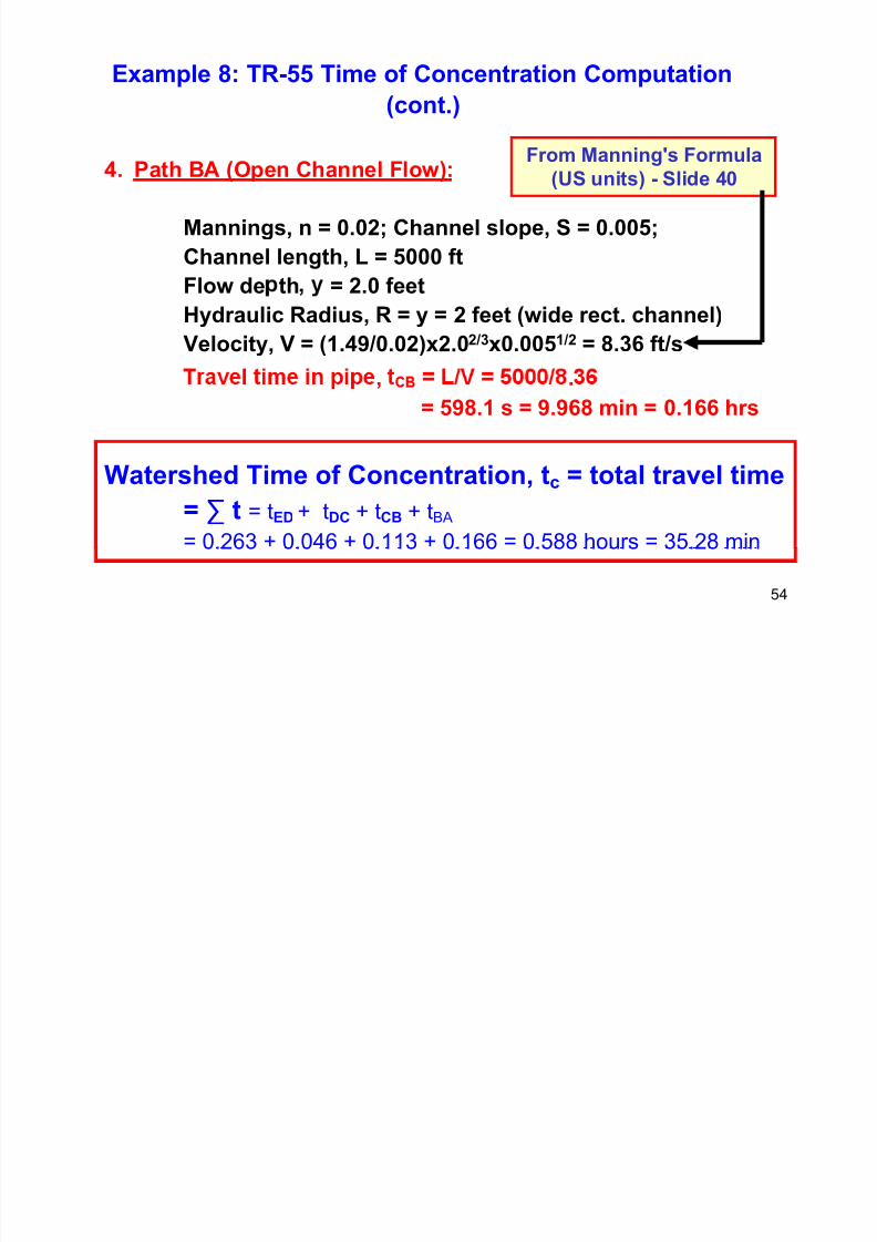
(cont.)
4. Path BA (Open Channel Flow):From Manning's Formula
(US units) - Slide 40
Mannings, n = 0.02; Channel slope, S = 0.005;
Channel length, L = 5000 ftFlow de th = 2.0 feet
Hydraulic Radius, R = y = 2 feet (wide rect. channel)
Velocity, V = (1.49/0.02)x2.02/3x0.0051/2 = 8.36 ft/s
, .
= 598.1 s = 9.968 min = 0.166 hrs
Watershed Time of Concentration, tc = total travel time= ∑ t = tED + tDC + tCB + tBA
= 0.263 + 0.046 + 0.113 + 0.166 = 0.588 hours = 35.28 min
54
Problem 5: SCS TR 55 Time of
7/21/2019 Pe Civil Hydrology Fall 2011
http://slidepdf.com/reader/full/pe-civil-hydrology-fall-2011 55/109
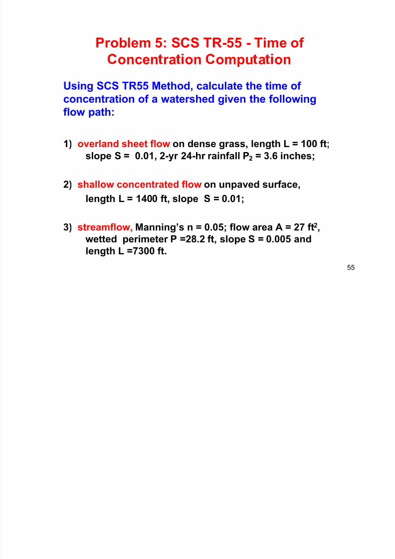
Problem 5: SCS TR-55 - Time of
oncen ra on ompu a on
Using SCS TR55 Method, calculate the time of
concentration of a watershed given the following
flow path:
1) overland sheet flow on dense grass, length L = 100 ft;
slope S = 0.01, 2-yr 24-hr rainfall P2 = 3.6 inches;
2) shallow concentrated flow on unpaved surface,
length L = 1400 ft, slope S = 0.01;
3) streamflow, Manning’s n = 0.05; flow area A = 27 ft2,
wetted perimeter P =28.2 ft, slope S = 0.005 and
55
length L =7300 ft.
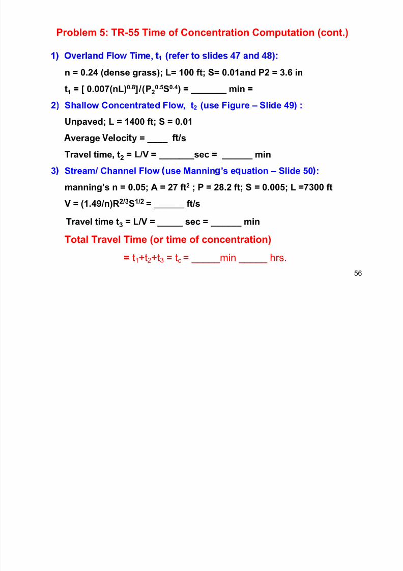
Problem 5: TR-55 Time of Concentration Computation (cont.)
7/21/2019 Pe Civil Hydrology Fall 2011
http://slidepdf.com/reader/full/pe-civil-hydrology-fall-2011 56/109
,
n = 0.24 (dense grass); L= 100 ft; S= 0.01and P2 = 3.6 in
t1 = [ 0.007(nL)0.8]/(P20.5S0.4) = _______ min =
2) Shallow Concentrated Flow, t2 (use Figure – Slide 49) :
Unpaved; L = 1400 ft; S = 0.01
verage e oc y = ____ s
Travel time, t2 = L/V = _______sec = ______ min
3 Stream/ Channel Flow use Mannin ’s e uation – Slide 50 :
manning’s n = 0.05; A = 27 ft2 ; P = 28.2 ft; S = 0.005; L =7300 ft
V = (1.49/n)R2/3S1/2 = ______ ft/s
Travel time t3 = L/V = _____ sec = ______ min
Total Travel Time (or time of concentration)
56
= t1+t2+t3 = tc = _____min _____ hrs.
SCS TR55 Method – Peak Discharge

7/21/2019 Pe Civil Hydrology Fall 2011
http://slidepdf.com/reader/full/pe-civil-hydrology-fall-2011 57/109
SCS TR55 Method Peak Discharge
Steps:
1. Compute watershed composite curve number CN;. , , ,
(inches) and Ia /P ratio;
3. Compute direct runoff volume Q (inches);
. , u .time of concentration, tc and Ia /P ratio from Figure inSlide 58 (or similar curve for Type I and III )
. , .
6. Compute peak discharge qp = qu Q A F
57
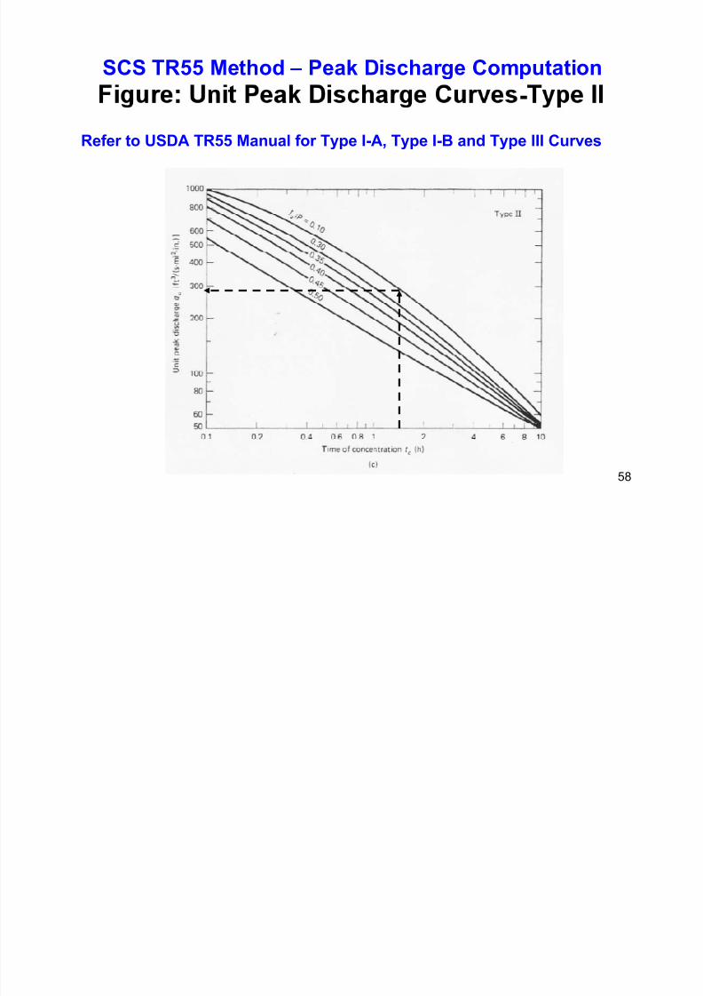
SCS TR55 Method – Peak Discharge Computation
7/21/2019 Pe Civil Hydrology Fall 2011
http://slidepdf.com/reader/full/pe-civil-hydrology-fall-2011 58/109
g p
- Refer to USDA TR55 Manual for Type I-A, Type I-B and Type III Curves
58
Example 9: TR 55 Computation of Peak Flow
7/21/2019 Pe Civil Hydrology Fall 2011
http://slidepdf.com/reader/full/pe-civil-hydrology-fall-2011 59/109
Example 9: TR-55 Computation of Peak Flow
s ng rap ca ea sc arge e o
• 250 acre (0.39 sq. miles) watershed;
• 25-year, 24hour Type II design rainfall P = 6 inches;
• watershed time of concentration, tc
= 1.50 hours;
• composite SCS Curve number CN = 75
• Neglect storage in lakes and ponds.
Compute the peak discharge qp.
59
Example 9: TR-55 Computation of Peak Flow
7/21/2019 Pe Civil Hydrology Fall 2011
http://slidepdf.com/reader/full/pe-civil-hydrology-fall-2011 60/109
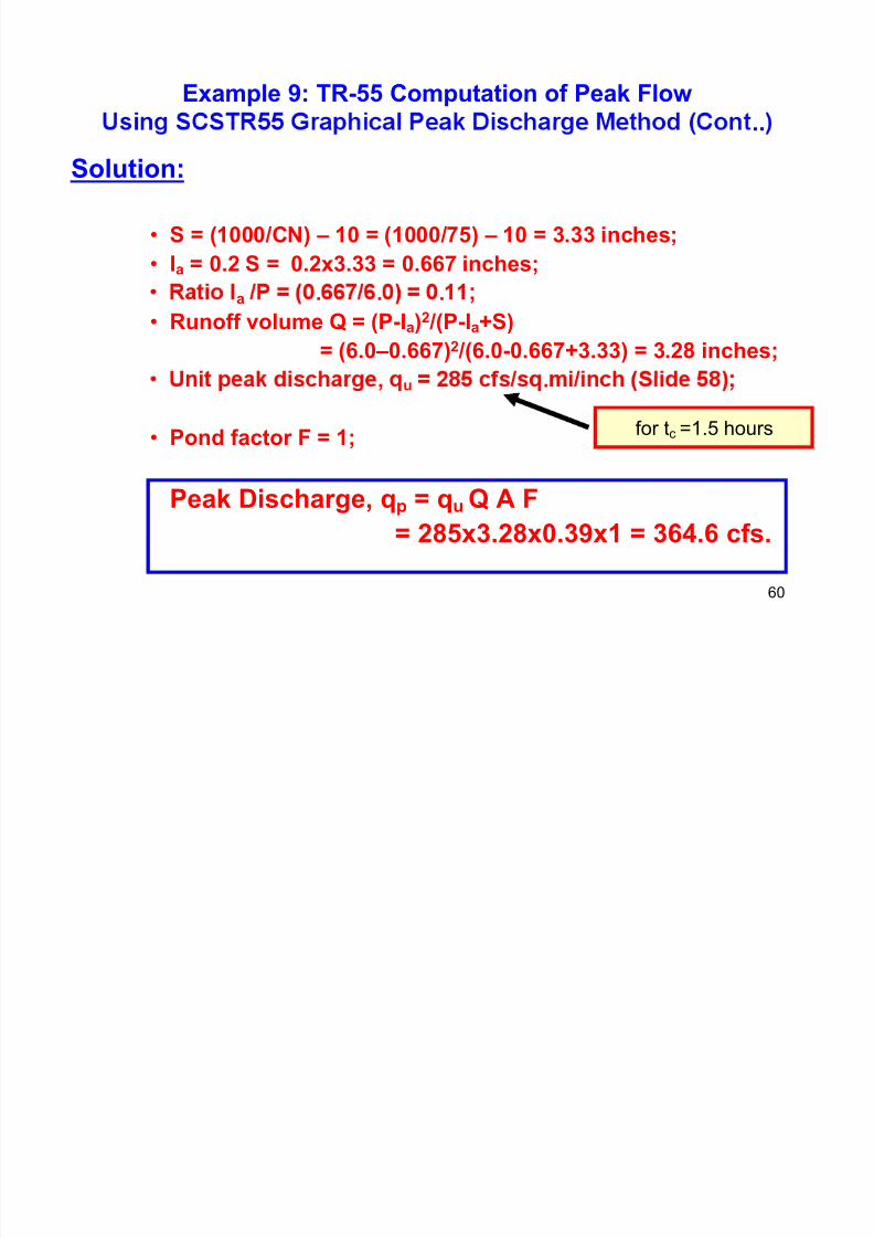
Example 9: TR 55 Computation of Peak Flow
..Solution:
• S = (1000/CN) – 10 = (1000/75) – 10 = 3.33 inches;
• Ia = 0.2 S = 0.2x3.33 = 0.667 inches;
a . . .
• Runoff volume Q = (P-Ia)2 /(P-Ia+S)
= (6.0–0.667)2 /(6.0-0.667+3.33) = 3.28 inches;
, u .
• Pond factor F = 1; for tc =1.5 hours
Peak Discharge, qp = qu Q A F
= 285x3.28x0.39x1 = 364.6 cfs.
60
Runoff Midsize Catchments
it H d h M th d
7/21/2019 Pe Civil Hydrology Fall 2011
http://slidepdf.com/reader/full/pe-civil-hydrology-fall-2011 61/109
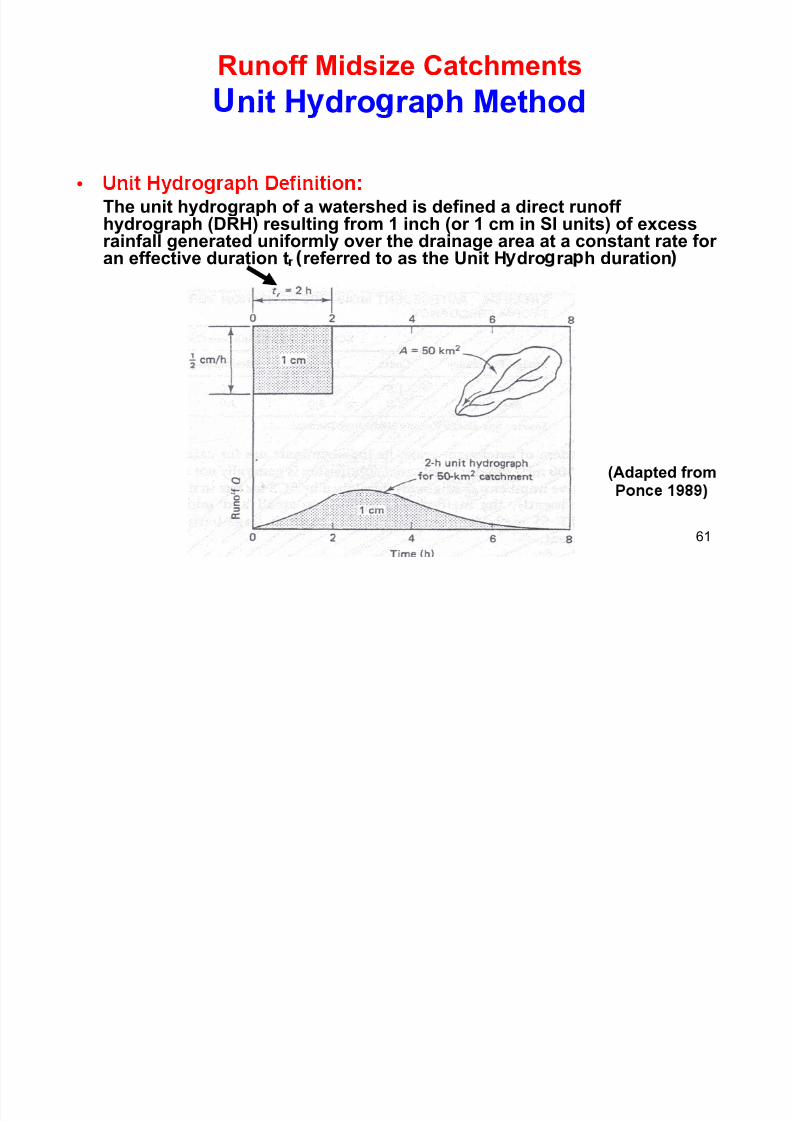
nit H dro ra h Method
• The unit hydrograph of a watershed is defined a direct runoff
hydrograph (DRH) resulting from 1 inch (or 1 cm in SI units) of excessrainfall generated uniformly over the drainage area at a constant rate foran effective duration t referred to as the Unit H dro ra h duration
(Adapted from
61
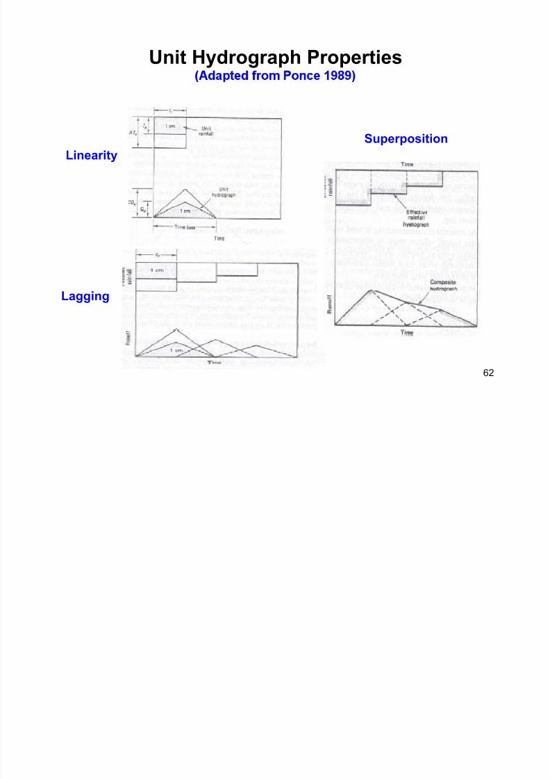
Unit Hydrograph Properties
7/21/2019 Pe Civil Hydrology Fall 2011
http://slidepdf.com/reader/full/pe-civil-hydrology-fall-2011 62/109
y g p p
Linearity
Superposition
Lagging
62
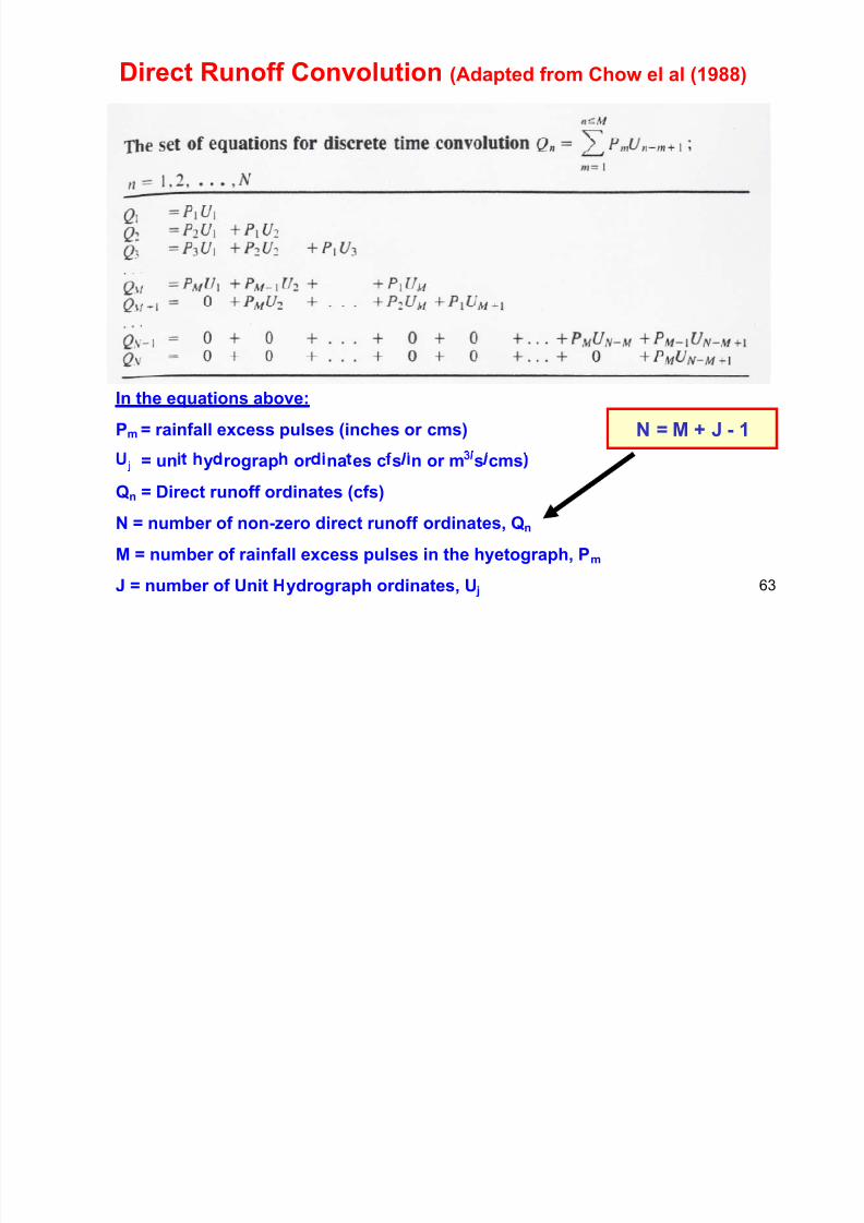
Direct Runoff Convolution (Adapted from Chow el al (1988)
7/21/2019 Pe Civil Hydrology Fall 2011
http://slidepdf.com/reader/full/pe-civil-hydrology-fall-2011 63/109
In the equations above:
Pm = rainfall excess pulses (inches or cms) N = M + J - 1
j = un y rograp or na es c s n or m s cms
Qn = Direct runoff ordinates (cfs)
N = number of non-zero direct runoff ordinates, Qn
63
M = number of rainfall excess pulses in the hyetograph, Pm
J = number of Unit Hydrograph ordinates, U j
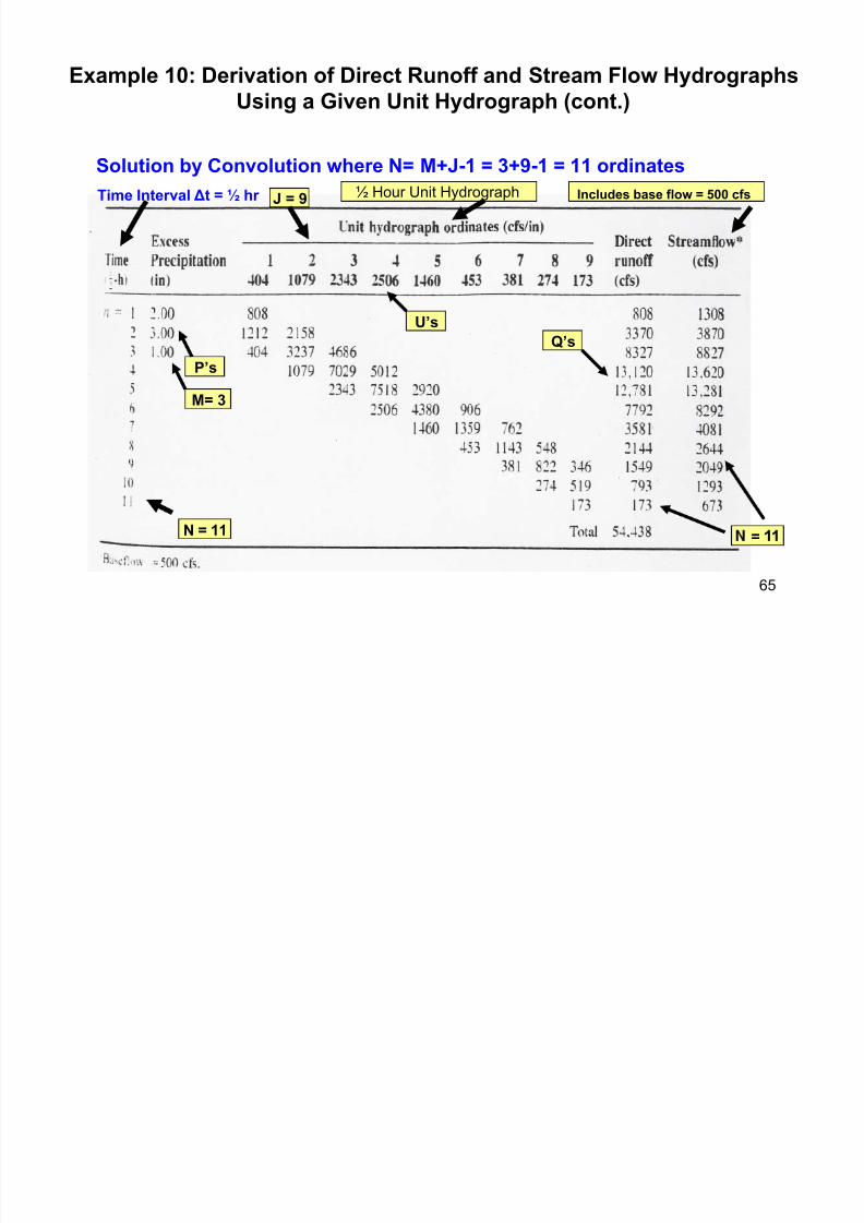
Example 10: Derivation of Direct Runoff and
7/21/2019 Pe Civil Hydrology Fall 2011
http://slidepdf.com/reader/full/pe-civil-hydrology-fall-2011 64/109
Streamflow H dro ra hs Usin a Given Unit
Hydrograph (Chow el al 1988)
• ½ hour unit hydrograph• Storm of 6 inches total rainfall excess de th with:
2 inches first half hour (P1),
3 inches in the second half hour (P2)
1 inch in the third half hour (P3)
• Base Flow = 500 cfs
•
Direct Runoff and the Streamflow Hydrograph.
64
Example 10: Derivation of Direct Runoff and Stream Flow Hydrographs
Using a Given Unit Hydrograph (cont )
7/21/2019 Pe Civil Hydrology Fall 2011
http://slidepdf.com/reader/full/pe-civil-hydrology-fall-2011 65/109
Using a Given Unit Hydrograph (cont.)
Solution by Convolution where N= M+J-1 = 3+9-1 = 11 ordinates
Time Interval Δt = ½ hr Includes base flow = 500 cfsJ = 9 ½ Hour Unit Hydrograph
P’s
U’s
Q’s
M= 3
=N = 11
65
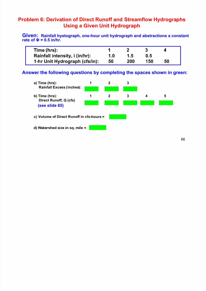
Problem 6: Derivation of Direct Runoff and Streamflow Hydrographs
Using a Given Unit Hydrograph
7/21/2019 Pe Civil Hydrology Fall 2011
http://slidepdf.com/reader/full/pe-civil-hydrology-fall-2011 66/109
Using a Given Unit Hydrograph
Given: Rainfall hyetograph, one-hour unit hydrograph and abstractions a constantrate of Φ = 0.5 in/hr.
me rs :
Rainfall intensity, i (in/hr): 1.0 1.5 0.5
1-hr Unit Hydrograph (cfs/in): 50 200 150 50
Answer the following questions by completing the spaces shown in green:
a) Time (hrs): 1 2 3
Rainfall Excess inches :
b) Time (hrs): 1 2 3 4 5
Direct Runoff, Q (cfs)
(see slide 65)
c) Volume of Direct Runoff in cfs-hours =
=
66
.

7/21/2019 Pe Civil Hydrology Fall 2011
http://slidepdf.com/reader/full/pe-civil-hydrology-fall-2011 67/109
.
Remember to Review the following
Appendix for:
1. Hydrologic Routing
2. Groundwater Hydrology – Well Hydraulics3. Additional examples on Unit Hydrograph
Good luck on the P.E. Exam
67
7/21/2019 Pe Civil Hydrology Fall 2011
http://slidepdf.com/reader/full/pe-civil-hydrology-fall-2011 68/109
1. Chow, Maidment, Mays, 1988. Applied Hydrology
2. Chow, ed. 1964. Handbook of Applied Hydrology
. , , . .
4. Freeze, Cherry, 1979. Groundwater
5. Maidment, ed. 1993. Handbook of Hydrology
6. Ponce, 1989. Engineering Hydrology
68
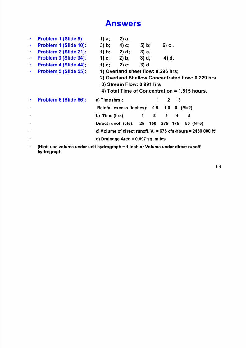
Answers
7/21/2019 Pe Civil Hydrology Fall 2011
http://slidepdf.com/reader/full/pe-civil-hydrology-fall-2011 69/109
• Problem 1 (Slide 9): 1) a; 2) a .• Problem 1 (Slide 10): 3) b; 4) c; 5) b; 6) c .
• Problem 2 (Slide 21): 1) b; 2) d; 3) c.
• .
• Problem 4 (Slide 44); 1) c; 2) c; 3) d.
• Problem 5 (Slide 55): 1) Overland sheet flow: 0.296 hrs;2) Overland Shallow Concentrated flow: 0.229 hrs
3) Stream Flow: 0.991 hrs
4) Total Time of Concentration = 1.515 hours.
• Problem 6 (Slide 66): a) Time (hrs): 1 2 3
• Rainfall excess (inches): 0.5 1.0 0 (M=2)
• b) Time (hrs): 1 2 3 4 5
• Direct runoff (cfs): 25 150 275 175 50 (N=5)
• c o ume o rect runo , d = c s- ours = , t
• d) Drainage Area = 0.697 sq. miles
• (Hint: use volume under unit hydrograph = 1 inch or Volume under direct runoff
h dro ra h
69
7/21/2019 Pe Civil Hydrology Fall 2011
http://slidepdf.com/reader/full/pe-civil-hydrology-fall-2011 70/109
APPENDIX A
H drolo ic Desi nComponents for
70
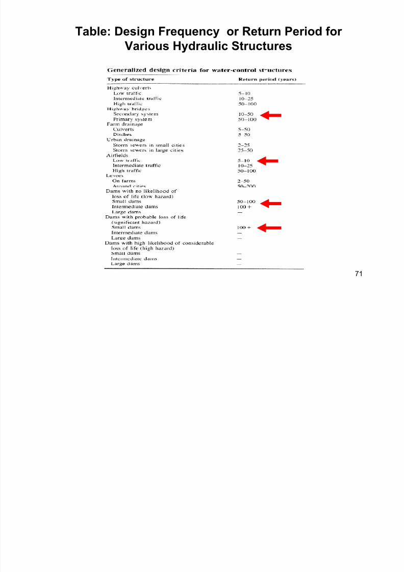
Table: Design Frequency or Return Period for
Various Hydraulic Structures
7/21/2019 Pe Civil Hydrology Fall 2011
http://slidepdf.com/reader/full/pe-civil-hydrology-fall-2011 71/109
71
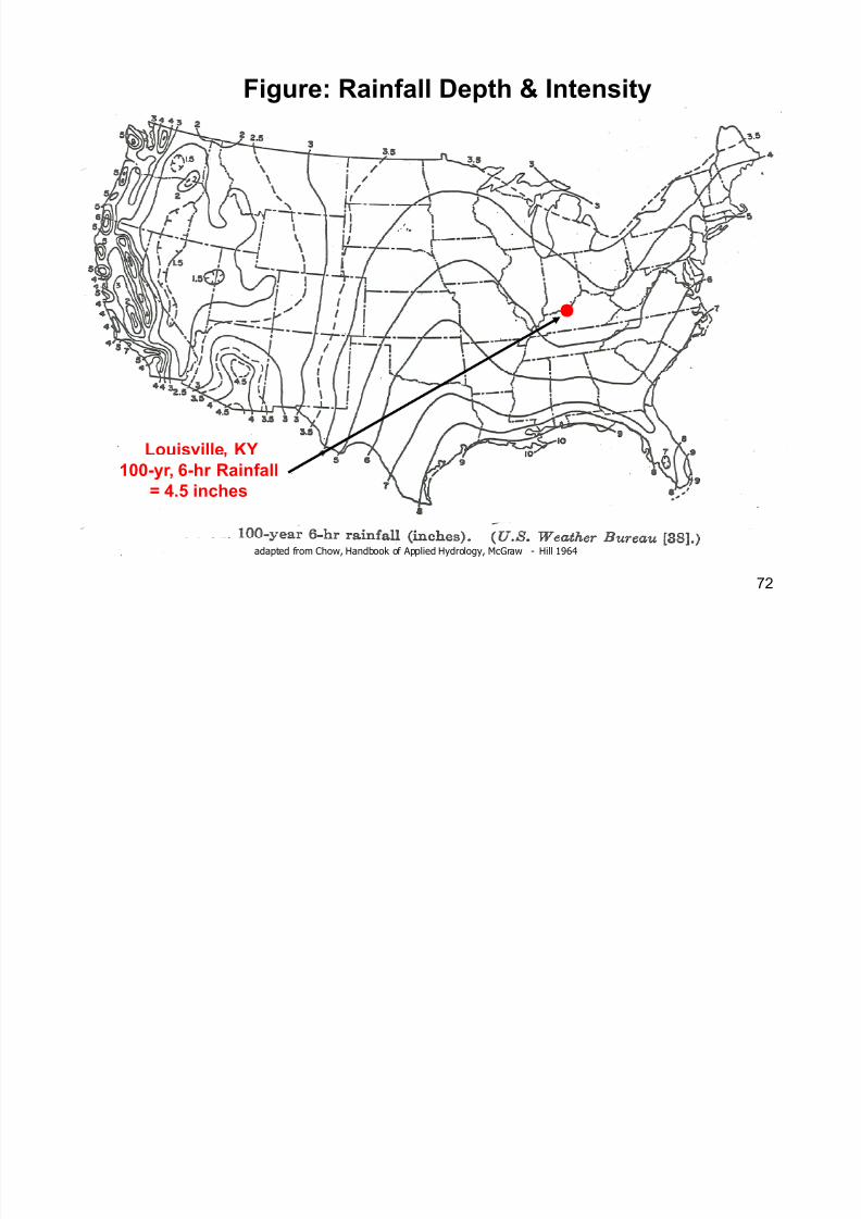
Figure: Rainfall Depth & Intensity
7/21/2019 Pe Civil Hydrology Fall 2011
http://slidepdf.com/reader/full/pe-civil-hydrology-fall-2011 72/109
Louisville KY
40
100-yr, 6-hr Rainfall
= 4.5 inches
72
adapted from Chow, Handbook of Applied Hydrology, McGraw - Hill 1964
Methods for Computing Time of

7/21/2019 Pe Civil Hydrology Fall 2011
http://slidepdf.com/reader/full/pe-civil-hydrology-fall-2011 73/109
g
Concentration
• Formulas
– Example: Kirpich, SCS Average Velocity Charts
• Approximate Velocities
73
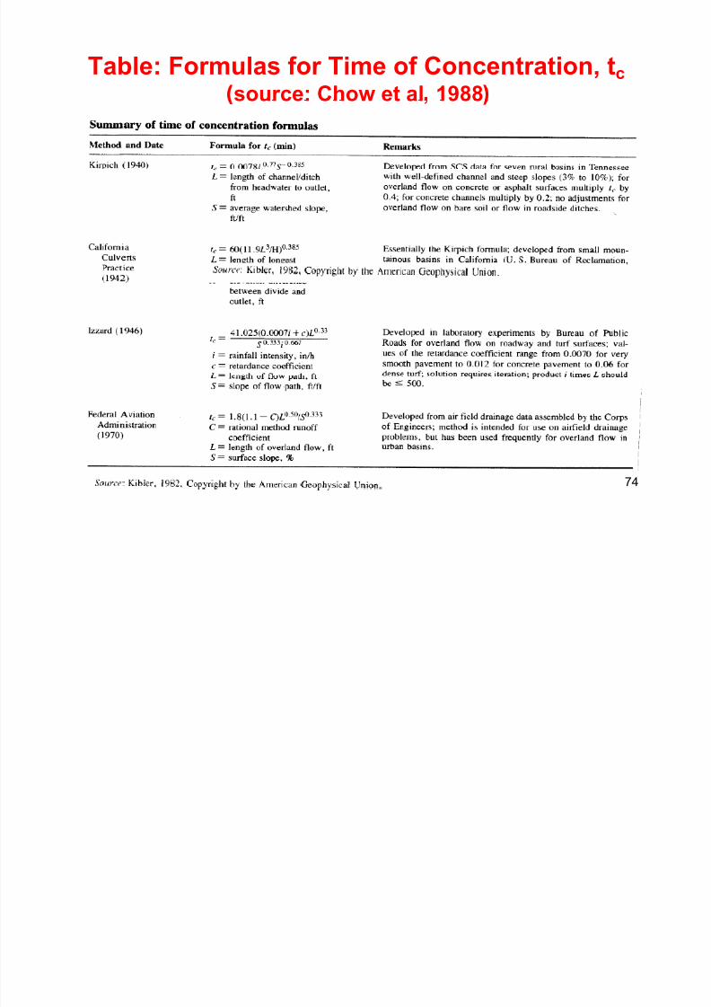
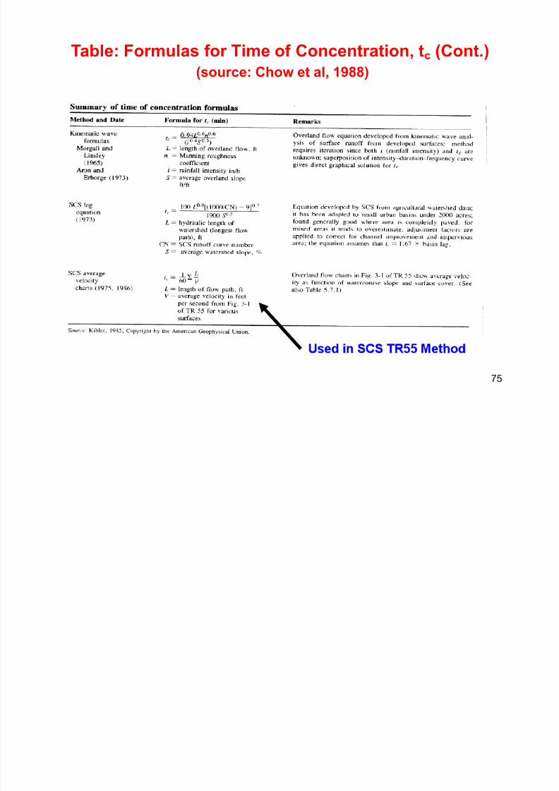
Table: Formulas for Time of Concentration, tc
source: Chow et al 1988
7/21/2019 Pe Civil Hydrology Fall 2011
http://slidepdf.com/reader/full/pe-civil-hydrology-fall-2011 74/109
source: Chow et al 1988
74
Table: Formulas for Time of Concentration, tc (Cont.)
(source: Chow et al, 1988)
7/21/2019 Pe Civil Hydrology Fall 2011
http://slidepdf.com/reader/full/pe-civil-hydrology-fall-2011 75/109
( )
75
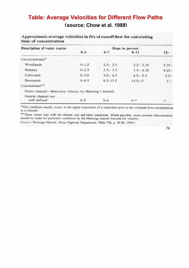
Table: Average Velocities for Different Flow Paths
source: Chow et al 1988
7/21/2019 Pe Civil Hydrology Fall 2011
http://slidepdf.com/reader/full/pe-civil-hydrology-fall-2011 76/109
76

7/21/2019 Pe Civil Hydrology Fall 2011
http://slidepdf.com/reader/full/pe-civil-hydrology-fall-2011 77/109
Hydrologic Routing
77
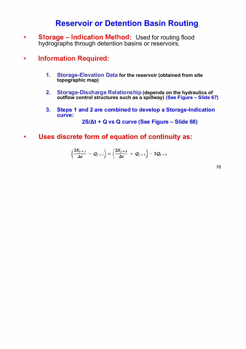
Reservoir or Detention Basin Routing
7/21/2019 Pe Civil Hydrology Fall 2011
http://slidepdf.com/reader/full/pe-civil-hydrology-fall-2011 78/109
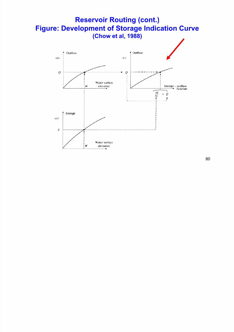
• orage – n ca on e o : Used for routing floodhydrographs through detention basins or reservoirs.
1. Storage-Elevation Data for the reservoir (obtained from sitetopographic map)
2. Storage-Discharge Relationship (depends on the hydraulics ofoutflow control structures such as a spillway) (See Figure – Slide 67)
3. Steps 1 and 2 are combined to develop a Storage-Indicationcurve:
2S/Δt + Q vs Q curve (See Figure – Slide 68)
• Uses discrete form of equation of continuity as:
78
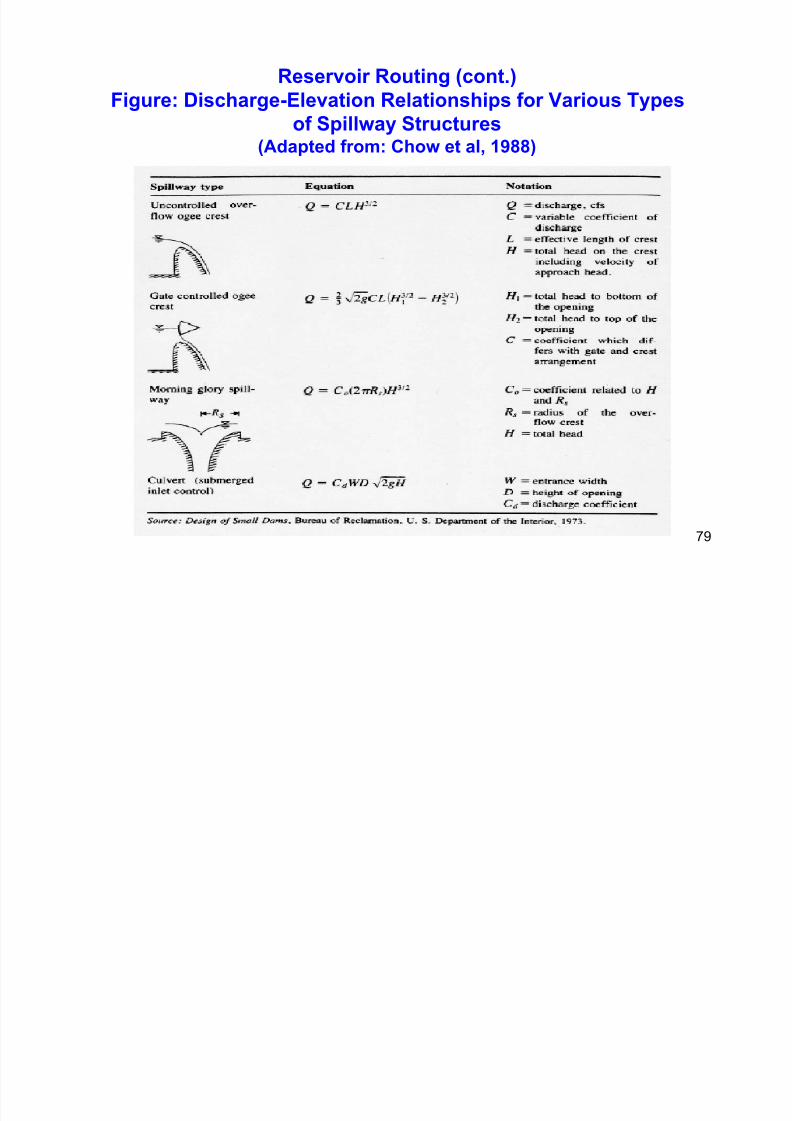
Reservoir Routing (cont.)
Figure: Discharge-Elevation Relationships for Various Types
7/21/2019 Pe Civil Hydrology Fall 2011
http://slidepdf.com/reader/full/pe-civil-hydrology-fall-2011 79/109
of Spillway Structures(Adapted from: Chow et al, 1988)
79
Reservoir Routing (cont.)
Figure: Development of Storage Indication Curve
7/21/2019 Pe Civil Hydrology Fall 2011
http://slidepdf.com/reader/full/pe-civil-hydrology-fall-2011 80/109
(Chow et al, 1988)
80
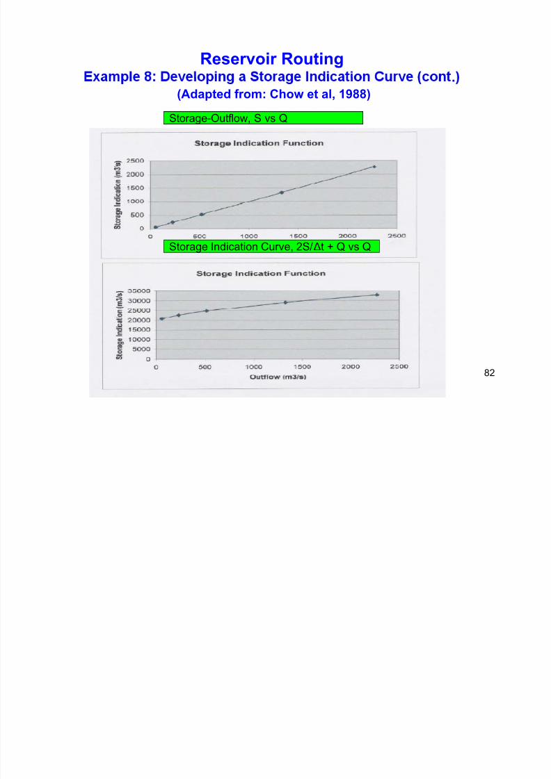
Reservoir Routing (cont.)
Example 8: Developing a Storage Indication Curve.

7/21/2019 Pe Civil Hydrology Fall 2011
http://slidepdf.com/reader/full/pe-civil-hydrology-fall-2011 81/109
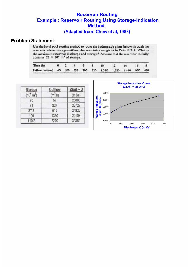
Problem Statement:
Stora e vs outflow characteristics for a ro osed reservoir are iven below.
Calculate the storage-outflow function 2S/Δt + Q vs Q for each of the tabulated
values if Δt = 2 hours. Plot a graph of the storage-outflow function.
________________________________________________________________________
orage, m : . .
Outflow, Q (m3 /s): 57 227 519 1330 2270
________________________________________________________________________
Solution:
81
Reservoir Routing.
7/21/2019 Pe Civil Hydrology Fall 2011
http://slidepdf.com/reader/full/pe-civil-hydrology-fall-2011 82/109
(Adapted from: Chow et al, 1988)
Storage-Outflow, S vs Q
Storage Indication Curve, 2S/ Δt + Q vs Q
82
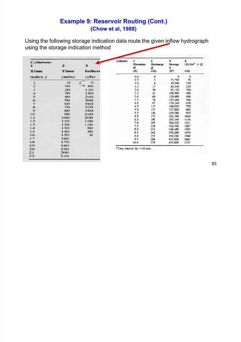
Example 9: Reservoir Routing (Cont.)
(Chow et al, 1988)
7/21/2019 Pe Civil Hydrology Fall 2011
http://slidepdf.com/reader/full/pe-civil-hydrology-fall-2011 83/109
Using the following storage indication data route the given inflow hydrographusing the storage indication method
83
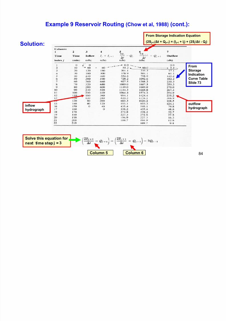
Example 9 Reservoir Routing (Chow et al, 1988) (cont.):
7/21/2019 Pe Civil Hydrology Fall 2011
http://slidepdf.com/reader/full/pe-civil-hydrology-fall-2011 84/109
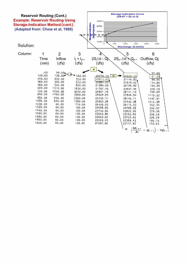
Solution:From Storage Indication Equation(2S j+1 /Δt + Q j+1) = (I j+1 + I j) + (2S j /Δt - Q j)
FromStorage
Indication
Curve Table
Slide 73
outflow
hydrographinflow
hydrograph
Solve this equation for
84
next t me step =
Column 5 Column 6
Reservoir Routing
Example : Reservoir Routing Using Storage-Indication
.
7/21/2019 Pe Civil Hydrology Fall 2011
http://slidepdf.com/reader/full/pe-civil-hydrology-fall-2011 85/109
(Adapted from: Chow et al, 1988)
Problem Statement:
Storage Indication Curve
(2S/dT + Q) vs Q
35000
i o n ,
s )
20000
25000
t o r g a e I n
d i c a
2 S / d t + Q
( m 3 /
85
15000
0 500 1000 1500 2000 2500
Discharge, Q (m3/s)
Reservoir Routing (Cont.)
Example: Reservoir Routing Using
Stora e-Indication Method cont. .
Storage Indication Curve
(2S/dT + Q) vs Q
35000
i o n ,
s )
i c a
( m 3
7/21/2019 Pe Civil Hydrology Fall 2011
http://slidepdf.com/reader/full/pe-civil-hydrology-fall-2011 86/109
(Adapted from: Chow et al, 1988)
15000
20000
25000
0 500 1000 1500 2000 2500
S t o r g a e I n d
2 S / d t + Q
1 2 3 4 5 6Time Inflow I j + I j+1 2S j/∆t - Qj 2S j+1/∆t + Q j+1 Outflow, Qj
o u on:
Column:
Discharge, Q (m3/s)
m n c s c s c s c s c s
+
=+
86
=
7/21/2019 Pe Civil Hydrology Fall 2011
http://slidepdf.com/reader/full/pe-civil-hydrology-fall-2011 87/109
Groundwater:
87
GROUND WATER HYDROLOGY
7/21/2019 Pe Civil Hydrology Fall 2011
http://slidepdf.com/reader/full/pe-civil-hydrology-fall-2011 88/109
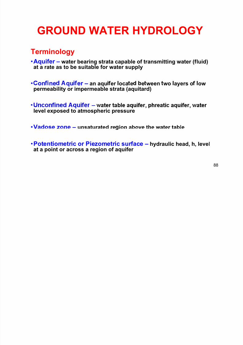
Terminology
•Aquifer – water bearing strata capable of transmitting water (fluid)at a rate as to be suitable for water supply
• on ne qu er – an aqu er oca e e ween wo ayers o owpermeability or impermeable strata (aquitard)
– , ,level exposed to atmospheric pressure
•Vadose zone – unsaturated re ion above the water table
•Potentiometric or Piezometric surface – hydraulic head, h, levelat a point or across a region of aquifer
88
Fundamental Principles
7/21/2019 Pe Civil Hydrology Fall 2011
http://slidepdf.com/reader/full/pe-civil-hydrology-fall-2011 89/109
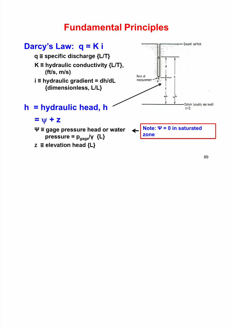
Darcy’s Law: q = K i
K ≡ hydraulic conductivity {L/T},
(ft/s, m/s)
i ≡ hydraulic gradient = dh/dL
{dimensionless, L/L}
h = hydraulic head, h
= + z
Ψ ≡ gage pressure head or waterpressure = pgage /γ {L}
Note: Ψ = 0 in saturated
zone
89
Fundamental Principles (cont.)
7/21/2019 Pe Civil Hydrology Fall 2011
http://slidepdf.com/reader/full/pe-civil-hydrology-fall-2011 90/109
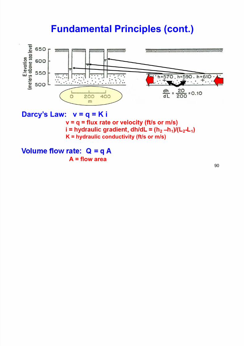
Darcy’s Law: v = q = K iv = q = flux rate or velocity (ft/s or m/s)
, 2 – 1 2- 1
K = hydraulic conductivity (ft/s or m/s)
= A = flow area
90
Well Hydraulics
Thi ’ St d St t S l ti
7/21/2019 Pe Civil Hydrology Fall 2011
http://slidepdf.com/reader/full/pe-civil-hydrology-fall-2011 91/109
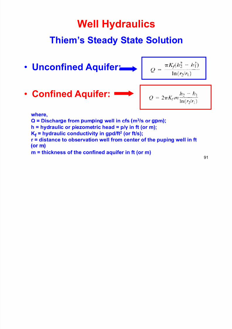
Thiem’s Steady State Solution
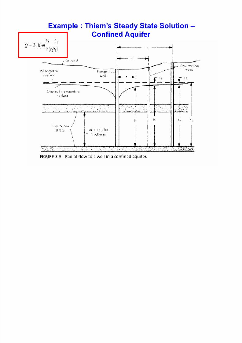
• Unconfined Aquifer:
• Confined Aquifer:
where,
Q = Dischar e from um in well in cfs m3 /s or m
h = hydraulic or piezometric head = p/γ in ft (or m);
Kf = hydraulic conductivity in gpd/ft2 (or ft/s);r = distance to observation well from center of the puping well in ft
m = thickness of the confined aquifer in ft (or m)91
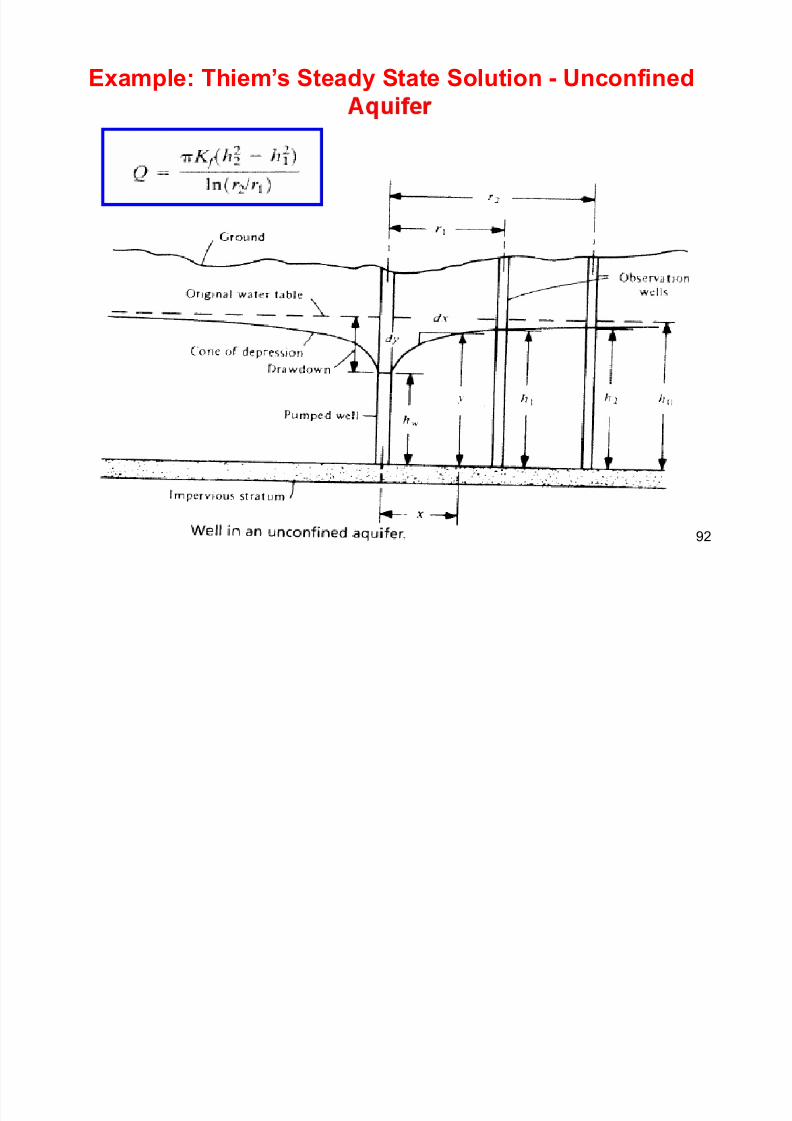
Example: Thiem’s Steady State Solution - Unconfined
7/21/2019 Pe Civil Hydrology Fall 2011
http://slidepdf.com/reader/full/pe-civil-hydrology-fall-2011 92/109
92
Example: Thiem’s Steady State
-
7/21/2019 Pe Civil Hydrology Fall 2011
http://slidepdf.com/reader/full/pe-civil-hydrology-fall-2011 93/109
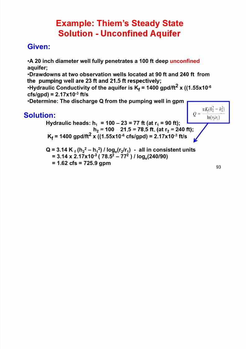
Given:
•A 20 inch diameter well fully penetrates a 100 ft deep unconfined
aquifer;
•Drawdowns at two observation wells located at 90 ft and 240 ft from
•Hydraulic Conductivity of the aquifer is Kf = 1400 gpd/ft2 x ((1.55x10⁻⁶
cfs/gpd) = 2.17x10⁻³ ft/s
•Determine: The discharge Q from the pumping well in gpm
Solution:Hydraulic heads: h1 = 100 – 23 = 77 ft (at r 1 = 90 ft);
= – = = . . .
Kf
= 1400 gpd/ft2 x ((1.55x10⁻⁶ cfs/gpd) = 2.17x10⁻³ ft/s
Q = 3.14 K f (h22 – h1
2) / loge(r 2 /r 1) - all in consistent units
93
= 3.14 x 2.17x10- ( 78.5 – 77 ) / loge(240/90)
= 1.62 cfs = 725.9 gpm
Example : Thiem’s Steady State Solution –
7/21/2019 Pe Civil Hydrology Fall 2011
http://slidepdf.com/reader/full/pe-civil-hydrology-fall-2011 94/109
94
Example : Thiem’s Steady State Solution –
P bl D t i th h d li d ti it K f t i
7/21/2019 Pe Civil Hydrology Fall 2011
http://slidepdf.com/reader/full/pe-civil-hydrology-fall-2011 95/109
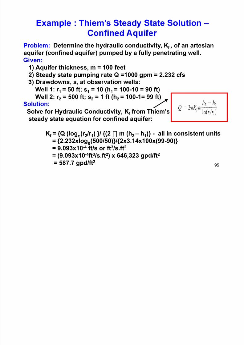
Problem: Determine the hydraulic conductivity, Kf , of an artesian
aquifer (confined aquifer) pumped by a fully penetrating well.
ven:
1) Aquifer thickness, m = 100 feet
2) Steady state pumping rate Q =1000 gpm = 2.232 cfs , ,
Well 1: r 1 = 50 ft; s1 = 10 (h1 = 100-10 = 90 ft)
Well 2: r 2 = 500 ft; s2 = 1 ft (h2 = 100-1= 99 ft)
Solve for Hydraulic Conductivity, Kf from Thiem’s
steady state equation for confined aquifer:
Kf = {Q (loge(r 2 /r 1) }/ {(2 ∏ m (h2 – h1)} - all in consistent units
= {2.232xloge(500/50)}/{2x3.14x100x(99-90)}= 9.093x10⁻⁴ ft/s or ft3 /s.ft2
95
= (9.093x10⁻⁴ft3 /s.ft2) x 646,323 gpd/ft2
= 587.7 gpd/ft2
Theis Unsteady State Solution
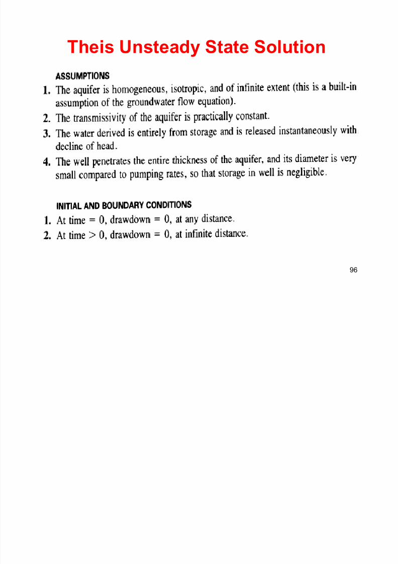
7/21/2019 Pe Civil Hydrology Fall 2011
http://slidepdf.com/reader/full/pe-civil-hydrology-fall-2011 96/109
96
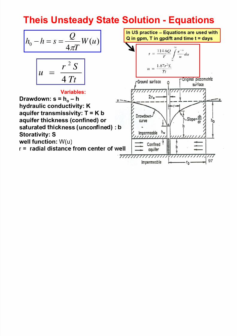
Theis Unsteady State Solution - Equations –
)(0 uWshh ==−
Q in gpm, T in gpd/ft and time t = days
7/21/2019 Pe Civil Hydrology Fall 2011
http://slidepdf.com/reader/full/pe-civil-hydrology-fall-2011 97/109
)(4
0 uW T
shhπ
gp , gp y
S r u
2
=
Variables:
Drawdown: s = ho – h
hydraulic conductivity: K
aquifer transmissivity: T = K b
aquifer thickness (confined) or
sa ura e c ness uncon ne :
Storativity: Swell function: W(u)
97
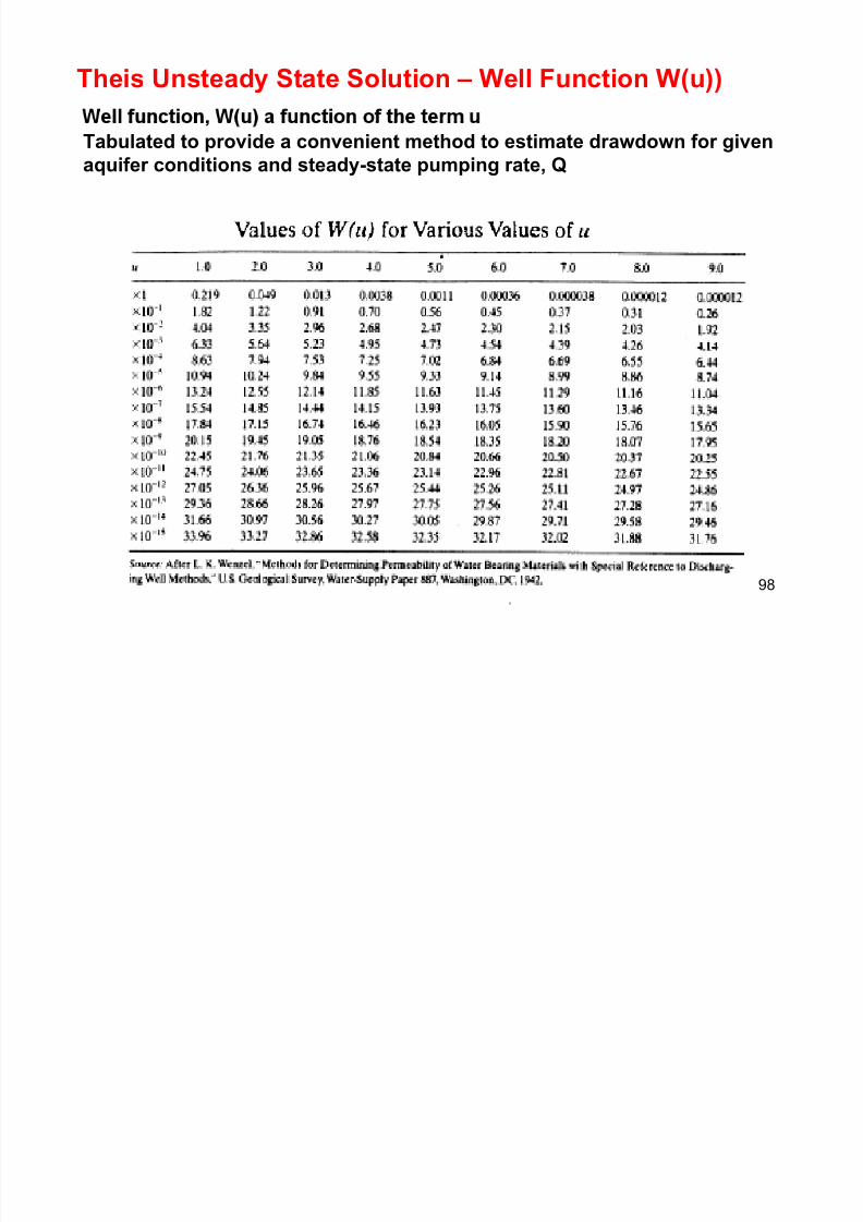
Theis Unsteady State Solution – Well Function W(u))
Tabulated to provide a convenient method to estimate drawdown for givenif diti d t d t t i t Q
7/21/2019 Pe Civil Hydrology Fall 2011
http://slidepdf.com/reader/full/pe-civil-hydrology-fall-2011 98/109
p gaquifer conditions and steady-state pumping rate, Q
98
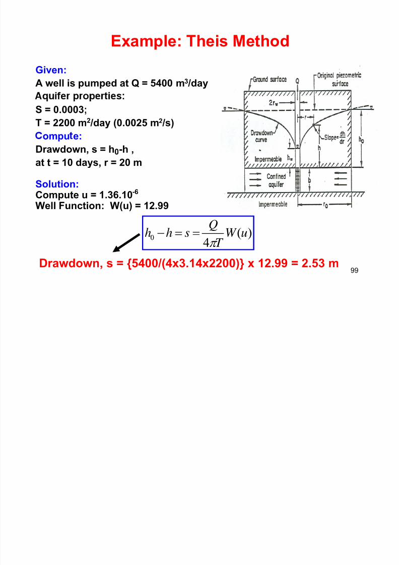
Example: Theis Method
Given:
7/21/2019 Pe Civil Hydrology Fall 2011
http://slidepdf.com/reader/full/pe-civil-hydrology-fall-2011 99/109
A well is pumped at Q = 5400 m3 /day
S = 0.0003;
T = 2200 m2 /day (0.0025 m2 /s)ompu e:
Drawdown, s = h0-h ,
at t = 10 days, r = 20 m
Solution:Compute u = 1.36.10-6
Well Function: W(u) = 12.99
)(4
0 uW T Qshhπ
==−
Drawdown, s = {5400/(4x3.14x2200)} x 12.99 = 2.53 m99
Problem 7: Drawdown by Theis method
Gi
7/21/2019 Pe Civil Hydrology Fall 2011
http://slidepdf.com/reader/full/pe-civil-hydrology-fall-2011 100/109
Given:
•The following information for a confined aquifer:
= 2
b) Storage coefficient S = 0.0005.
c) Aquifer thickness = 200 feet
d Well delivers a dischar e of Q = 500 m
•Determine the drawdown at an observation well located 150 feet
=
equations.
100
(Note: 1 cfs = 448 gpm).
7/21/2019 Pe Civil Hydrology Fall 2011
http://slidepdf.com/reader/full/pe-civil-hydrology-fall-2011 101/109
Unit Hydrograph
101
Exam le: Unit H dro ra h Derivation
P bl St t t D t i 1/2h U it H d h i th

7/21/2019 Pe Civil Hydrology Fall 2011
http://slidepdf.com/reader/full/pe-civil-hydrology-fall-2011 102/109
Problem Statement: Determine 1/2hr Unit Hydrograph using the
excess rainfall hyetograph and Direct Runoff Hydrograph shown
in the Table below. (Adapted from Chow el al (1988)
102
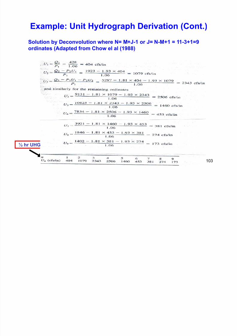
Example: Unit Hydrograph Derivation (Cont.)
Solution by Deconvolution where N= M+J-1 or J= N-M+1 = 11-3+1=9di t (Ad t d f Ch l l (1988)
7/21/2019 Pe Civil Hydrology Fall 2011
http://slidepdf.com/reader/full/pe-civil-hydrology-fall-2011 103/109
ordinates (Adapted from Chow el al (1988)
½ hr UHG
103
Problem : Derivation of Direct Runoff and Streamflow
Hydrographs Using a Given Unit Hydrograph
7/21/2019 Pe Civil Hydrology Fall 2011
http://slidepdf.com/reader/full/pe-civil-hydrology-fall-2011 104/109
Problem Statement:
104
Problem : Derivation of Direct Runoff and Streamflow Hydrographs
Using a Given Unit Hydrograph (cont.)
Solution:
7/21/2019 Pe Civil Hydrology Fall 2011
http://slidepdf.com/reader/full/pe-civil-hydrology-fall-2011 105/109
105
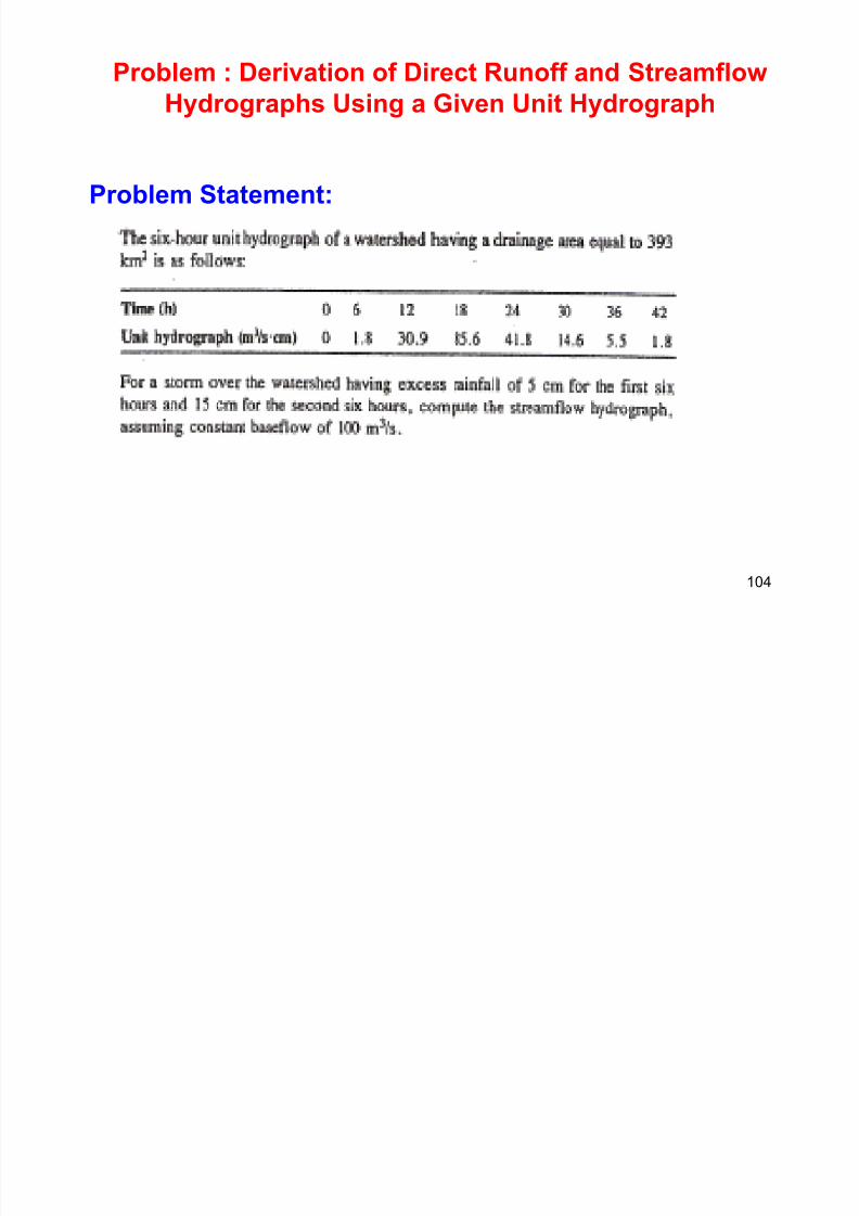
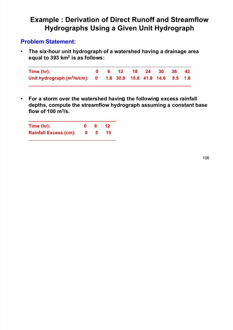
Example : Derivation of Direct Runoff and Streamflow
Hydrographs Using a Given Unit Hydrograph
Problem Statement:
7/21/2019 Pe Civil Hydrology Fall 2011
http://slidepdf.com/reader/full/pe-civil-hydrology-fall-2011 106/109
• The six-hour unit hydrograph of a watershed having a drainage area
equal to 393 km is as follows:
_______________________________________________________________
Time (hr): 0 6 12 18 24 30 36 42 . . . . . . .
_______________________________________________________________
• For a storm over the watershed havin the followin excess rainfall
depths, compute the streamflow hydrograph assuming a constant base
flow of 100 m3 /s.
__________________________________
Time (hr): 0 6 12
Rainfall Excess (cm): 0 5 15 __________________________________
106
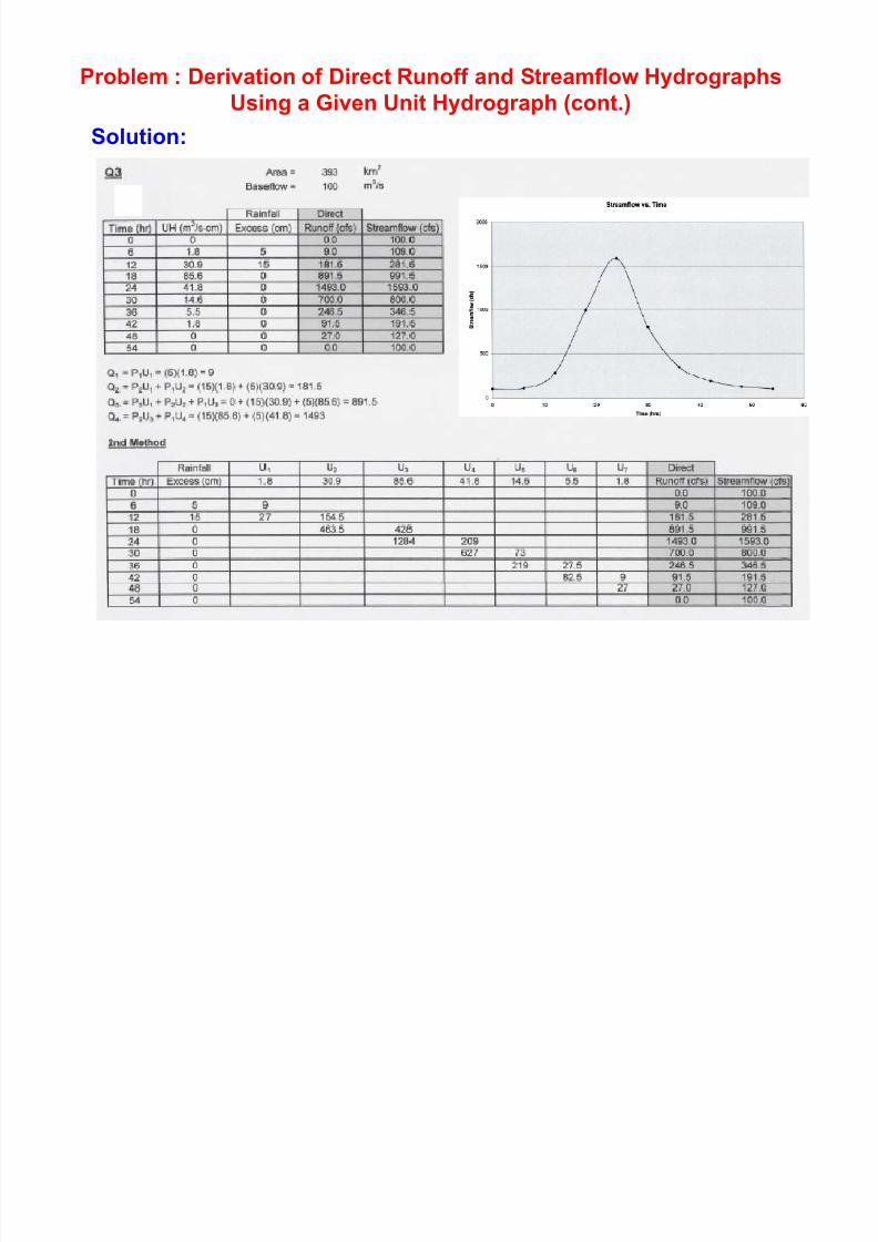
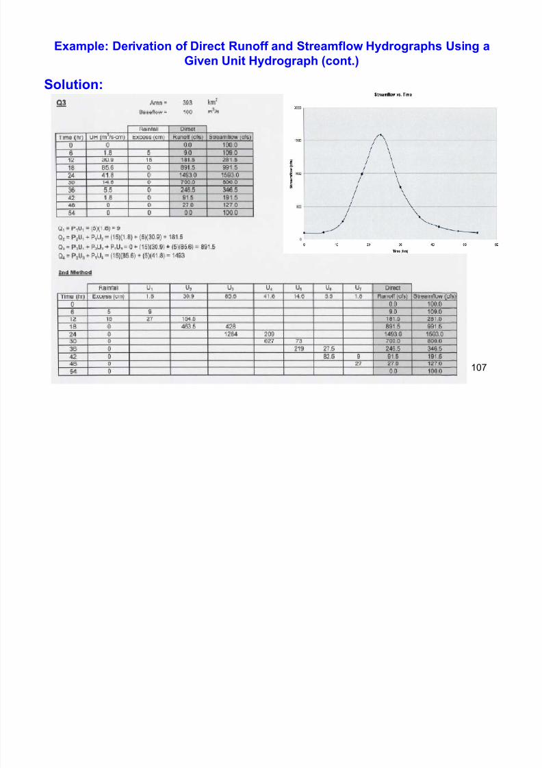
Example: Derivation of Direct Runoff and Streamflow Hydrographs Using a
Given Unit Hydrograph (cont.)
Solution:
7/21/2019 Pe Civil Hydrology Fall 2011
http://slidepdf.com/reader/full/pe-civil-hydrology-fall-2011 107/109
107
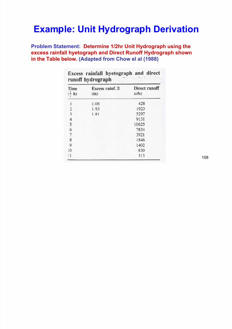
Exam le: Unit H dro ra h Derivation
Problem Statement: Determine 1/2hr Unit Hydrograph using the
7/21/2019 Pe Civil Hydrology Fall 2011
http://slidepdf.com/reader/full/pe-civil-hydrology-fall-2011 108/109
Problem Statement: Determine 1/2hr Unit Hydrograph using the
excess rainfall hyetograph and Direct Runoff Hydrograph shown
in the Table below. (Adapted from Chow el al (1988)
108
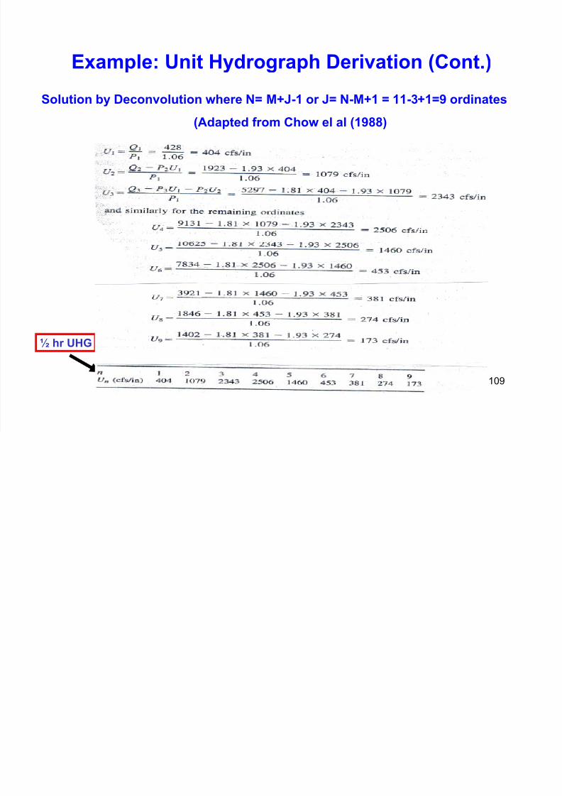
Example: Unit Hydrograph Derivation (Cont.)
Solution by Deconvolution where N= M+J-1 or J= N-M+1 = 11-3+1=9 ordinates
7/21/2019 Pe Civil Hydrology Fall 2011
http://slidepdf.com/reader/full/pe-civil-hydrology-fall-2011 109/109
(Adapted from Chow el al (1988)
½ hr UHG
109


![[Hydrology] groundwater hydrology david k. todd (2005)](https://img.pdfslide.net/doc/110x75/55a8e6001a28ab6c2f8b4687/hydrology-groundwater-hydrology-david-k-todd-2005-55b0d9a792c06.jpg)