Embed Size (px)
Citation preview

On relations between extreme value statistics, extreme random matrices andPeak-Over-Threshold method
Jacek Grela∗
LPTMS, CNRS, Univ. Paris-Sud, Universite Paris-Saclay, 91405 Orsay, France
Maciej A. Nowak†
M. Smoluchowski Institute of Physics and Mark Kac Complex Systems Research Centre,Jagiellonian University, Lojasiewicza 11, 30–348 Krakow, Poland
(Dated: November 20, 2017)
Using the thinning method, we explain the link between classical Fisher-Tippett-Gnedenko clas-sification of extreme events and their free analogue obtained by Ben Arous and Voiculescu in thecontext of free probability calculus. In particular, we present explicit examples of large random ma-trix ensembles, realizing free Weibull, free Frechet and free Gumbel limiting laws, respectively. Wealso explain, why these free laws are identical to Balkema-de Haan-Pickands limiting distributionfor exceedances, i.e. why they have the form of generalized Pareto distributions and derive a simpleexponential relation between classical and free extreme laws.
I. INTRODUCTION
Random matrix theory is one of the most universal probabilistic tools in physics and in several multidisciplinaryapplications [1]. In the limit when the size of the matrix tends to infinity, random matrix theory bridges to freeprobability theory, which can be viewed as an operator valued (i.e. non-commutative) analogue of the classical theoryof probability [2, 3]. Both calculi exhibit striking similarities. Wigner’s semicircle law can be viewed as an analogue ofnormal distribution, Marcenko-Pastur spectral distribution for Wishart matrices is an analogue of Poisson distributionin classical probability calculus, and Bercovici-Pata bijection [4] is an analogue of Levy stable processes classificationfor heavy-tailed distributions. It is therefore tempting to ask the question, how far can we extend the analogiesbetween these two formalisms?
Extreme value theory in classical probability is the prominent application of probability calculus for several problemsseeking extreme values for large number of random events. Its power comes from the fact, that it has universalprobabilistic laws - according to Fisher-Tippett-Gnedenko classification of extreme values [5], only three genericstatistics of extremes saturate all possibilities - Gumbel distribution, Frechet distribution and Weibull distribution.Beyond applications of extreme value theory in physics in the theory of disordered systems [6], seminal applicationsinclude insurance, finances, hydrology, mechanics, biology, computer science, and several others [7]. This is preciselyalso the domain of applications of random matrix theory. This coincidence raises a natural question - do we have ananalogue of extreme values limiting distributions for the spectra of very large random matrices, i.e does Fisher-Tippett-Gnedenko classification exists in free probability? The positive answer to this crucial question was provided more thena decade ago by Ben Arous and Voiculescu [8]. Using operator techniques, they have proven that free probability theoryhas also three limiting extreme distributions - free Gumbel, free Frechet and free Weibull distribution. Although thedomains of attraction are the same as in their classical counterparts, the functional form of these limiting distributionswas however different. In all three cases, there are represented by certain generalized Pareto distribution. Surprisingly,these were identical to the threefold classification of exceedances in extreme value theory, i.e. they were representedby Balkema-de Haan-Pickands [13, 14] classification in classical probability theory.
In this paper, we shed some light on these unexpected links. In the first section, we introduce a thinning approach toorder statistics, which allows us to re-express extreme values calculus in an intuitive way. This reformulation permitsus to understand the operator-valued approach of [8] in terms of the concepts of classical probability. Then weshow how this reformulation is equivalent to Peak-Over-Threshold method, which explains, why the free probabilityextreme laws are governed by generalized Pareto distributions. We stress that extreme laws in both calculi havestriking similarities - they admit not only the same domains of attraction, but even the same form of centering and
∗ [email protected]† [email protected]
arX
iv:1
711.
0345
9v2
[m
ath-
ph]
17
Nov
201
7

2
Thinning
Extreme Value Statistics
Extreme Matrix Statistics
Asymptotic Thinning
Classic Extreme Laws Free Extreme Laws POT Extreme Laws
Exponentiation
Peak-Over-Threshold
Generalized Pareto
FIG. 1. Flow diagram relating the thinning approach to different aspects of extreme value theory.
scaling constants. We address these coinciding features by finding a relation between classic and free/Peak-Over-Threshold extreme laws by an exponentiation. Finally, we exemplify our results by explicit calculations of extremelaws for random matrix ensembles, representing free Weibull, free Frechet and free Gumbel spectral laws, respectively.All aforementioned links between different phenomena investigated in the article are shown in the diagram in FigureI.
II. ORDER AND EXTREME VALUE STATISTICS
Extremes of random numbers are described by order statistics. Given a set of m random variables {x1, · · · , xm},we rearrange them in an ascending order {x(1), · · · , x(m)}. As an example, for a set of such variables the followinginequalities holds true
x(1) ≤ x(2) ≤ · · · ≤ x(m−1) ≤ x(m)
x3 ≤ xm−1 ≤ · · · ≤ x6 ≤ x2.
Typically one is interested in the extreme events and studies a particular element in the ordered set {x(1), · · · , x(m)}– either the largest x(m) or the smallest one x(1). One can study also the distributions of a subset of the ordered set– the n largest or smallest values.
In all these cases, the cumulative distribution function (or CDF) for the k-th order statistic x(k) of a sample of mvariables is given by:
P(m)(x(k) < x) =⟨θ(x− x(k)
)⟩P
=
m∑i=k
∑{σ}
∫ x
−∞dxσ(1) · · ·
∫ x
−∞dxσ(i) · · ·︸ ︷︷ ︸
i
∑{δ}
∫ ∞x
dxδ(1) · · ·∫ ∞x
dxδ(m−i)︸ ︷︷ ︸m−i
P (x1, ..., xm),
(1)
where P (x1, ..., xm) is the joint probability distribution function (PDF) of the not-ordered set of variables {x1, ..., xm},∑{σ} is the summation over i permutations of m indices and
∑{δ} is m− i permutations of remaining m− i elements.
Derivation of the above formula is straightforward when one realizes that in order for the variable to be a k-th orderstatistics x(k), its CDF P(m)(x(k) < x) comprises of all cases where at most m− k variables (i.e. 0, 1, 2 up to m− k)

3
are larger than x (the group of∫∞x
integrals) and the remaining k numbers are smaller than x (forming the group of∫ x−∞ integrals).
In the simplest case of identically and independently distributed (or i.i.d.) variables P (x1, ..., xm) =∏mi=1 p(xi) we
find∫ x−∞ p(t)dt = F (x) and
∫∞xp(t)dt = 1− F (x) which produces a well-known CDF:
P(m)(x(k) < x) =
m∑i=k
(m
i
)[F (x)]
i[1− F (x)]
m−i(2)
since∑{σ} =
(mi
)and
∑{δ} =
(m−im−i
)= 1. In particular, the distribution function of the largest value for k = m is
just P(m)(x(m) < x) = [F (x)]m
.
1. Thinning approach to order statistics
We describe a thinning procedure applied to order statistics. Consider the following problem – draw m i.i.d.variables {x1, · · · , xm} from parent PDF p(x) and CDF F (x), pick out the n largest ones {x(m) · · ·x(m−n+1)} andlook at their statistics. What will be the resulting probability density function (or PDF) and cumulative distribution
function (or CDF)? We find the thinned CDF F(m)k of the n largest values selected out of m values as a normalized
sum of n terms given by Eq. (2):
F(m)k (x) =
1
n
m∑i=m−n+1
P(m)(x(i) < x) (3)
with k = mn and the corresponding thinned PDF is found by differentiation p
(m)k (x) = d
dxF(m)k (x):
p(m)k (x) =
1
n
d
dx
m∑i=m−n+1
P(m)(x(i) < x). (4)
By using Eq. (2) and ddxP
(m)(x(i) < x) = m(m−1i−1)p(x) [F (x)]
i−1[1− F (x)]
m−i, the PDF reads
p(m)k (x) =
m
np(x)
[1−
m−n∑i=1
(m− 1
i− 1
)[F (x)]
i−1[1− F (x)]
m−i
], (5)
where the summation boundaries were changed by using an identity∑mi=1
(m−1i−1)
[F (x)]i−1
[1− F (x)]m−i
= 1. Cru-
cially, the presented approach is a generalization of the usual extreme value statistics (or EVS) as thinned CDF/PDFgiven by Eqs. (3) and (4) reduce to EVS counterparts for n = 1 (or k = m). Besides this special case, we considerlimit m,n→∞ with fixed ratio k = m/n where the sum in the thinned PDF of Eq. (5) is asymptotically given by
m−n∑i=1
(m− 1
i− 1
)[F (x)]
i−1[1− F (x)]
m−i ∼
{0, F (x) > α
1, F (x) < α, m, n→∞, and
m
nfixed, (6)
with α = k−1k and the details of this calculation are provided in App. A. We use the Heaviside theta function to
re-express Eq. (6) and write down a simple asymptotic thinned PDF pk(x) = limm,n→∞
p(m)k=m
n(x) as:
pk(x) = kp(x)θ(F (x)− α), (7)
where F (x) and p(x) are the parent CDF and PDF respectively. The definition Fk(x) =x∫−∞
dx′pk(x′) of the asymptotic
thinned CDF gives:
Fk(x) = k(F (x)− α)θ(F (x)− α). (8)
Interpretation of both asymptotic thinned PDF pk and CDF Fk is clear – picking n largest values out of m doesnot modify the shape of the parent distribution p(x) but truncates it up to a point x∗ such that F (x∗) = α. Thepoint x∗ is known in statistics as the last of the k-quantile and gives the point where the fraction of values smallerthan x∗ is α = k−1
k . Importantly, since the large n,m limit was taken the fraction α takes all real number between(0, 1). In the following Sections we continue with relating the asymptotic thinned PDF and CDF to random matricesand Peak-Over-Threshold method.

4
III. EXTREME MATRIX STATISTICS
Extreme statistics of matrices were introduced in general operator language in Refs. [8, 9] and the special case ofextreme matrices were discussed in detail in Ref. [10]. We first introduce these findings in what follows.
To quantify extremal features in a set of observables, a notion of order is indispensable – a characteristic of beingeither largest or smallest is needed. Although a natural inequality operator exists for real numbers (giving rise tostandard EVS) for other objects it may not be the case. Already the complex plane lacks such an ordering; z1 ≥ z2 fortwo complex numbers does not bear any natural interpretation. In particular, defining the order either by modulusor by comparing real and imaginary parts separately does not produce satisfactory results. To assess such problemsin full generality, the order theory developed two notions of partially and totally ordered set. A partially ordered setis endowed with a binary relation ≤ satisfying three conditions satisfied by all elements a, b, c in the set:
• a ≤ a (reflexivity)
• a ≤ b and b ≤ a → a = b (antisymmetry)
• a ≤ b and b ≤ c → a ≤ c (transitivity)
A totally ordered set is a partially ordered set with an additional property – for each a, b
• either a ≤ b or b ≤ a (totality)
Given these definitions, we reconsider the example of complex numbers – modulus-based ordering does not satisfythe antisymmetry property and the real-and-imaginary-based ordering is only partial. We are now ready to defineextreme cases of more exotic objects like matrices.
We focus on extremes in the space of Hermitian matrices. Consider finite N×N matrices with N distinct eigenvaluesλi and eigenvectors |ψi〉. A spectral order is defined for Hermitian matrices Ha, Hb in terms of the spectral projections:
Ha ≺ Hb ←→ E(Ha; [t,∞)) ≤ E(Hb; [t,∞)),
where the spectral projection for a matrix Ha is given by E(Ha; [t,∞)) =∑Ni=1 |ψi〉 〈ψi| θ(λi−t) and A ≤ B operation
on the space of Hermitian projections is defined as ∀x : xT (B − A)x ≥ 0. With this ordering, the definitions of min(∧) and max (∨) operations of Hermitian matrices are:
Ha ∧Hb ←→ E(Ha ∧Hb; [t,∞)) = E(Ha; [t,∞)) ∧ E(Hb; [t,∞)),
Ha ∨Hb ←→ E(Ha ∨Hb; [t,∞)) = E(Ha; [t,∞)) ∨ E(Hb; [t,∞)).(9)
If the matrices are random, the max operation becomes especially simple – given 2N eigenvalues of Ha, Hb, we pickout of them the N largest eigenvalues and form the spectrum of Ha∨Hb. Since a random matrix is unitarily invariant,eigenvalues alone fully specify the matrix. We state the maximal law for asymptotically large matrices given in Refs.[8, 10].
Define the asymptotic eigenvalue PDF (or the spectral density) of the random matrixH as ρH(t) = limN→∞
1N
⟨N∑i=1
δ(λi − t)⟩
where the average is taken wrt. a prescribed matrix PDF. Asymptotic eigenvalue CDF is in turn given by
FH(x) =x∫−∞
dtρH(t) of Ha, Hb. The asymptotic eigenvalue CDF of the maximum Ha ∨ Hb of two random ma-
trices Ha, Hb is given by:
FHa∨Hb(x) = max(0, FHa(x) + FHb(x)− 1).
As a special case, for a maximum of k i.i.d. matrices each with eigenvalue CDF FH(x) we find:
FH∨k(x) = max(0, kFH(x)− (k − 1)), (10)
where H∨k = H ∨ ... ∨H︸ ︷︷ ︸k terms
.

5
1. GUE case
It is instructive to show the spectrum of extremal matrices as given by Eq. (10) on a classic example. We computeboth eigenvalue PDF and CDF in the simplest case of Gaussian Unitary Ensemble where the matrix is drawn froma Gaussian distribution P (H)dH ∼ exp
(−N2 TrH2
)dH. The asymptotic eigenvalue PDF is given by the celebrated
Wigner’s semicircle law:
ρH(t) =1
2π
√4− t2. (11)
The corresponding eigenvalue CDF is given by
FH(x) =1
2+
1
4πx√
4− x2 +1
πarcsin
x
2. (12)
k=5
k=20
k=80ρH
vk
k=150
k=300
k=500
k=600
k=700
k=900
0.5 1.0 1.5 2.0
2
4
6
8
10
1.90 1.95 2.00 2.05
5
10
15
20
25
30
35
1.94 1.96 1.98 2.00 2.02 2.04
10
20
30
40
50
ρHvk ρH
vk
FIG. 2. Analytical (lines) and numerical (points) density of eigenvalues ρH∨k of the maximum matrix H∨k = H1 ∨H2 ∨ ..Hkwhere each Hi is of size 500× 500 and drawn from an Gaussian Unitary Ensemble and the ordering in the space of matrices isdefined by Eq. (9).
Using Eq. (10) and the above eigenvalue CDF, we compute the k-maximal CDF and the corresponding PDF bydifferentiation ρH∨k(x) = d
dxFH∨k(x). The resulting formula is again a semicircle however truncated to an interval(x−, 2):
ρH∨k(x) =k
2π
√4− x2, x ∈ (x−, 2), (13)
with an approximate boundary at x− ∼ 2−(3π2k
) 23 , obtained by imposing the normalization condition
∫ 2
x−ρH∨k(x)dx =
1.In Fig. 1 we present how the density behaves for different values of k – the distribution retains its shape shape in
all cases and becomes truncated into an interval (x−, 2). Moreover, for values of k ∼ 1000 we observe a deviationfrom the formula (13) – numerical distribution seem to develop a tail for x > 2 and is smoothened near x ∼ x−.
2. Equivalence between extreme matrices and the thinning method
We show how the extremal law for random matrices given by Eq. (10) is expressible as the thinning procedureintroduced in Sec. II 1. We rewrite the asymptotic thinning CDF given by Eq. (8):
Fk(x) = (kF (x)− (1− k))θ
(F (x)− 1− k
k
),
then, since θ(af) = θ(f) for a > 0 and max(0, f) = fθ(f), we have
Fk(x) = max(0, kF (x)− (1− k)).

6
There is an exact correspondence with the CDF given by Eq. (10). The parent CDF F (x) and asymptotic thinningCDF Fk(x) corresponds to the single random matrix CDF FH(x) and the k-maximal CDF FH∨k(x) respectively. Thisequivalence is given formally by the formula
FH∨k(x) = Fk(x). (14)
The matrix interpretation of the thinning method is understood by the following replacements:
• n,m (sample sizes) → N,M (matrix sizes)
• values → eigenvalues
• parent PDF p(x)/CDF F (x) → eigenvalue PDF ρH(x)/CDF FH(x)
a. Equivalence in the GUE case. We relate the extremal eigenvalue PDF to the asymptotic thinning PDF foundin Eq. (7) in the previous example of Gaussian Unitary Ensemble. By making replacements as in the above list,the thinning procedure is picking N largest eigenvalues out of M = kN eigenvalues drawn from ρH(x) which readilycoincides with the extremal law for matrices given by (13). We see it also in the formulas itself, Eq. (7) gives theasymptotic thinned PDF:
pk(x) = kρH(x)θ(FH(x)− α).
which agrees with Eq. (13) as kρH(x) = k2π
√4− x2. The Heaviside theta function gives the appropriate truncation
at FH(x∗) = α equivalent to∫ x∗−∞ ρH(x)dx = α = 1− 1
k . Since∫∞−∞ ρH(x)dx = 1, we find∫ ∞
x∗
kρH(x)dx = 1,
which is the normalization condition for the PDF ρH∨k given by Eq. (13). We conclude that x− = x∗ and consequentlyEq. (13) is recreated. The same calculation can be done to retrieve the CDF FH∨k given by Eq. (12).
All above considerations are true in the limit when the matrix sizes grow to infinity M,N →∞. This corresponds tothe free probability regime in which extreme matrix laws are valid. Importantly however, it is also possible to considerthe maximum principle also for finite matrices. In this case, the thinning method as described in Sec. II 1 no longerapplies as the eigenvalues are correlated and no longer drawn from a semicircle law. The correlations necessitatesthe use of the general formula given by Eq. (1) with P consisting of k eigenvalue PDFs and construct a correlatedthinning framework. Although the problem is harder, it is a promising direction through Coulomb gas techniques asproven useful in extracting extreme value statistics of highly correlated PDFs of eigenvalues (see Refs. [11, 12]).
IV. LINKING THINNING APPROACH AND PEAK-OVER-THRESHOLD METHOD
We turn to investigate an apparent connection between the thinning approach and Peak-Over-Threshold method asalready signalled in the initial work [8] on extreme matrices. The method is closely related to the notion of exceedanceswhich arise conditioned on the event that the random variable X is larger than some threshold u. For t ≥ u, theexceedance distribution function F[u](t) is then
F[u](t) = P(X < t|X > u) =P(X < t,X > u)
P(X > u)=F (t)− F (u)
1− F (u),
where we used the usual definition of conditional probability P(A|B) = P(A,B)/P(B) and parent CDF F (x). ThePeak-Over-Threshold method (or POT) developed in Refs. [14, 15] in turn looks at excess distribution functions ofevents X above some threshold u:
PPOT(X < u+ t|X > u) =F (u+ t)− F (u)
1− F (u). (15)
An excess of t is therefore a variant of the exceedance shifted by the threshold u itself, i.e. F[u](t+ u).In the following we provide a connection between POT method and the thinning approach. It is evident that both
methods study extremes – POT method looks at values above some threshold whereas the thinning apporach focuses

7
on a fraction k of largest values drawn from the sample of m observations. To establish the link, it suffices to relatethe POT threshold u to the thinning fraction k:
F (u) = 1− 1
k, (16)
with a known parent CDF F (x). This one-to-one relation dictates where one should position the threshold in orderto capture a fraction k of values in the sample. This relation is strict in the limit of large samples as only then theinter-sample fluctuations vanish. By the same reason, this relation makes sense for any real value of k.
We show now that both asymptotic thinned CDF and PDF given by Eqs. (8) and (7) respectively are related tothe POT excess distribution function PPOT and its derivative:
PPOT(X < u+ t|X > u) = Fk(u)(u+ t),
d
dtPPOT(X < u+ t|X > u) = pk(u)(u+ t),
(17)
where k(u) = 11−F (u) follows from the relation (16). By Eq. (8), the thinned CDF reads:
Fk(u)(u+ t) = k(u)
(F (u+ t)− 1 +
1
k(u)
)θ
(F (u+ t)− 1 +
1
k(u)
),
and by simply computing F (u+ t)− 1 + 1k(u) = F (u+ t)− F (u) and θ(F (u+ t)− F (u)) = θ(t) is rewritten as
Fk(u)(u+ t) =F (t+ u)− F (u)
1− F (u)θ(t),
which recreates the POT excess distribution function given by Eq. (15) given an implicit assumption that t > 0. Thisexpression is also exactly that of Df. 7.2 given in Ref. [8]. By similar computation one can show the PDF equivalencestated in Eq. (17) as
pk(u)(u+ t) =1
1− F (u)p(t+ u)θ(t),
where p(x) is the parent PDF. On the other hand, from the POT excess distribution function given by Eq. (15) wearrive at the same formula with the help of d
dtF (u+ t) = p(u+ t).
V. EXTREME LAWS OF VALUES, MATRICES AND POTS
Up to now, a close relation between extreme matrix statistics, Peak-Over-Threshold method and the thinningapproach was established. We investigate these links further from the point of view of extreme laws.
a. Classic extreme laws. We first revise the classic extreme laws arising when inspecting the distribution of thelargest value x(m) in the sample of m i.i.d. variables drawn from parent PDF p(x). An m-independent form of themaximal CDF Fmax(x) exists:
limm→∞
P(m)(x(m) < am + bmx) = Fmax(x), (18)
with m dependent constants am and bm representing centering and scaling respectively. There exist three limitingforms of Fmax(x) depending on the properties of the parent PDF as summarized in Tab. I (see Ref. [16] for apedagogical review).
The thinning approach encompasses these classic extreme laws as the special case k = m of Eq. (3) is P(x(m) <
x) = F(m)m (x).
b. Free extreme laws. Hihgly similar free (or matrix) extreme laws exist for the CDF of noncommutative (or free)random variables defined as the limit of the formula given by Eq. (10):
limk→∞
FH∨k(ak + bkx) = F free(x). (19)
with some scaling and centering constants ak, bk. The classic and free extreme laws are highly similar – they admit thesame domains of attraction, constants ak, bk and properties of the parent distributions. The expressions for extremeCDF’s are however different and summarized in Tab. II.

8
name Gumbel Frechet Weibull
properties ofparent PDF p(x)
tails falls off fasterthan any power of x
p(x) falls off as ∼ x−(γ+1)
and is infinitep(x) is finite, p(x) = 0 for x > x+
p(x) ∼ (x− x+)−γ−1
maximal CDF FmaxI (x) = exp
(−e−x
), x ∈ R Fmax
II (x) =
{0 , x < 0
exp(−x−γ
), x > 0
FmaxIII (x) =
{exp (−(−x)γ) , x < 0
1 , x > 0
an F−1(1− 1/n) 0 x+bn F−1(1− 1/(ne))− an F−1(1− 1/n) x+ − F−1(1− 1/n)
TABLE I. Table summarizing three classic extreme laws of Gumbel, Frechet and Weibull. Functional inverse of the parentCDF F is denoted by F−1.
name free/POT Gumbel free/POT Frechet free/POT Weibull
CDF Ffree/POTI (x) =
{0 , x < 0
1− e−x , x > 0F
free/POTII (x) =
{0 , x < 1
1− x−γ , x > 1F
free/POTIII (x) =
0 , x < −1
1− (−x)γ , x ∈ (−1, 0)
1 , x > 0
examples Free Gauss (ex. 6) Free Cauchy γ = 1 (ex. 4) Wigner’s semicircle γ = 3/2 (ex. 1)Free Levy-Smirnov γ = 1/2 (ex. 5) Marcenko-Pastur γ = 3/2 (ex. 2)
Free Arcsine γ = 1/2 (ex. 3)
TABLE II. Table summarizing free extreme laws and POT extreme laws along with concrete examples computed in Sec. V A 1.
c. POT extreme laws. Lastly, the Peak-Over-Threshold method produces a highly similar family of extreme lawunder the name of generalized Pareto distribution (see Ref. [13]). By definition (15), the limiting distribution reads:
limu→∞
PPOT(X < u+ au + bux|X > u) = FPOT(x),
for some constants au, bu which although different than in the classic and free cases, we can fix them by demandingthat extreme-matrix and POT limiting distributions are exactly the same FPOT(x) = F free(x). This is possible asthe constants are not unique. Moreover, from the point of view of previously derived equivalencies this is hardly asurprise - both free and POT extreme laws ought to be related as both are expressed by the same extremal PDF andCDF given by Eqs. (7) and (8) respectively.
Relation between the constants are found by
F free(x) = limk→∞
FH∨k(ak + bkx) = limk→∞
Fk(ak + bkx) = limu→∞
Fk(u)(ak(u) + bk(u)x
),
and using a well-known limit composition theorem: if limk→∞
fk = c, limu→∞
k(u) = ∞ and fk is continuous then
limu→∞
fk(u) = c. On the other hand, we find
FPOT(x) = limu→∞
PPOT(X < u+ au + bux|X > u) = limu→∞
Fk(u)
(u+ au + bux
),
which gives the relations between the constants:
FPOT(x) = F free(x) −→
{u+ au = ak(u)bu = bk(u)
. (20)
As was mentioned before, all three laws in the POT approach are typically expressed in terms of the generalizedPareto distribution Gβ(x):
Gβ≥0(x) =
{0, x < 0,
1− (1 + βx)−1β , x > 0,
and Gβ<0(x) =
0, x < 0,
1− (1 + βx)−1β , x ∈
(0,− 1
β
),
1, x > − 1β .
where limβ→0
(1− (1 + βx)−
1β
)= 1 − e−x. We find FPOT
I (x) = G0(x), FPOTII (x) = G1/γ(γ(x − 1)) and FPOT
III (x) =
G−1/γ(γ(x+ 1)) as can be seen also in Tab. II.

9
A. Relating classical and free/POT extreme laws via exponentiation
Although classical and free/POT extreme CDFs have different functional forms, they seem to be related by astriking expression
F free(x) ≈ 1 + lnFmax(x), or
Fmax(x) ≈ exp(F free(x)− 1
),
(21)
Such relation between the POT extreme and classical EVS has been observed in classical probbaility, see e.g. [7].Unfortunately, this relation is valid only for the functional forms (see Tabs. I and II) and not for whole functions astheir domains do not simply match up. In what follows we derive a slightly modified formula (21) with valid treatmentof domains by using the thinning method. This derivation highlights the bijection between free and classical extremestatistics.
The classic extreme laws Fmax are found from the extremal CDF given by Eq. (2)
P(m)m (x) = [F (x)]
mθ(F (x)) (22)
with the parent CDF F (x). The step function is added freely as the parent CDF is always a positive function. Onthe other hand, the free extreme laws F free arise from the asymptotic thinned CDF given by Eq. (8):
Fm(x) = m
(F (x)− 1 +
1
m
)θ
(F (x)− 1 +
1
m
),
where we set k → m for clarity. We formally solve above equation for F (x):
F (x) = 1 +1
m
(Fm(x)
Tm(x)− 1
)and let Tm(x) = θ
(F (x)− 1 + 1
m
)be the step function. We plug it back to Eq. (22), set x→ am+bmx with constants
given in Tab. I and consider the limit m→∞ to obtain the classic extreme law CDF according to Eq. (18):
Fmax(x) = limm→∞
P(m)m (am + bmx) = lim
m→∞
(θ(F (am + bmx))
[1 +
1
m
(Fm(am + bmx)
Tm(am + bmx)− 1
)]m). (23)
The ratio Fm/Tm in this formula is in turn expressed asymptotically by free extreme law CDF Eq. (19) and stepfunction T (x):
limm→∞
Fm(am + bmx)
Tm(am + bmx)=F free(x)
T (x), (24)
Thus, both step functions t(x), T (x) admit m-independent form given by
T (x) = limm→∞
θ
(F (am + bmx)− 1 +
1
m
),
t(x) = limm→∞
θ(F (am + bmx)).(25)
After plugging these definitions back into Eq. (23), we use finally the exponentiation formula limm→∞
(1 + x/m)m = ex
and the corrected formula (21) relating free and classic extreme laws reads
Fmax(x) = t(x) exp
(F free(x)
T (x)− 1
), (26)
where step functions t and T are defined in Eq. (25). Based on explicitly calculated examples in Sec. V A 1, wepropose the form for these functions:
• t(x) = θ(x) if the parent CDF belongs to the Frechet domain and t(x) = 1 if parent CDF belongs to eitherGumbel or Weibull domains whereas
• T (x) = θ(x+ α) with α = −1 for Frechet domain, α = 0 for Gumbel domain and α = 1 for Weibull domain.
10
To support the form of T (x), we rewrite the free CDFs of Tab. II with the use of step functions:
• Gumbel domain gives F freeI (x) = θ(x)(1− e−x),
• Frechet domain gives F freeII (x) = θ(x− 1)(1− x−γ),
• Weibull domain gives F freeIII (x) = θ(x+ 1) [1− θ(−x)(−x)γ ].
and observe how in all three above formulas, there is a corresponding T (x) step function present and cancelled in theratio.
1. Examples
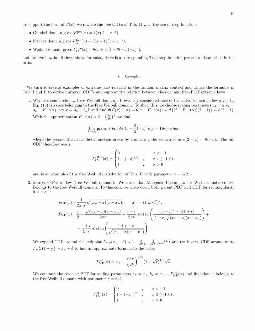
We turn to several examples of extreme laws relevant in the random matrix context and utilize the formulae inTab. I and II to derive universal CDF’s and support the relation between classical and free/POT extreme laws.
1. Wigner’s semicircle law (free Weibull domain). Previously considered case of truncated semicircle law given byEq. (13) is a case belonging to the Free Weibull domain. To show this, we choose scaling parameters ak = 2, bk =ak − F−1(α), set x = ak + bkx and find θ(F (x) − α) = θ(x − F−1(α)) = θ
((2− F−1(α))(x+ 1)
)= θ(x + 1).
With the approximation F−1(α) ∼ 2−(3π2k
) 23 we find:
limk→∞
pk(ak + bkx)bkdx =3
2(−x)
12 θ(x+ 1)θ(−x)dx,
where the second Heaviside theta function arises by truncating the semicircle as θ(2 − x) = θ(−x). The fullCDF therefore reads:
FGUEIII (x) =
0 , x < −1
1− (−x)3/2 , x ∈ (−1, 0)
1 , x > 0
,
and is an example of the free Weibull distribution of Tab. II with parameter γ = 3/2.
2. Marcenko-Pastur law (free Weibull domain). We check that Marcenko-Pastur law for Wishart matrices alsobelongs to the free Weibull domain. To this end, we write down both parent PDF and CDF for rectangularity0 < r < 1:
ρMP(x) =1
2πrx
√(x+ − x)(x− x−), x± = (1±
√r)2,
FMP(x) =1
2+
√(x+ − x)(x− x−)
2πr+
1− r2πr
arctan
((1− r)2 − x(1 + r)
(1− r)√
(x+ − x)(x− x−)
)+
− 1 + r
2πrarctan
(1 + r − x√
(x+ − x)(x− x−)
).
We expand CDF around the endpoint FMP(x+ − δ) ∼ 1− 23π
1(1+√r)2r3/4
δ3/2 and the inverse CDF around unity
F−1MP
(1− 1
k
)∼ x+ − δ to find an approximate formula to the latter
F−1MP(α) ∼ x+ −(
3π
2k
)2/3
(1 +√r)4/3
√r.
We compute the rescaled PDF for scaling parameters ak = x+, bk = x+ − F−1MP(α) and find that it belongs tothe free Weibull domain with parameter γ = 3/2:
FMPIII (x) =
0 , x < −1
1− (−x)3/2 , x ∈ (−1, 0)
1 , x > 0
.
11
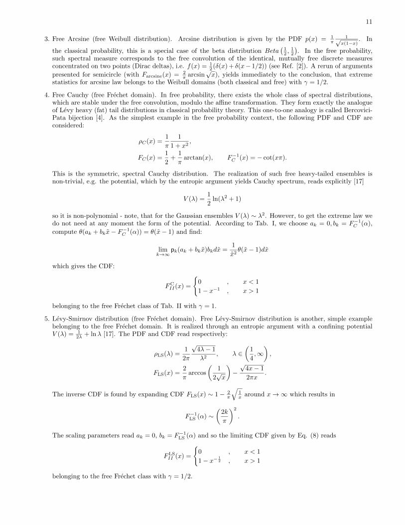
3. Free Arcsine (free Weibull distribution). Arcsine distribution is given by the PDF p(x) = 1π
1√x(1−x)
. In
the classical probability, this is a special case of the beta distribution Beta(12 ,
12
). In the free probability,
such spectral measure corresponds to the free convolution of the identical, mutually free discrete measuresconcentrated on two points (Dirac deltas), i.e. f(x) = 1
2 (δ(x) + δ(x− 1/2)) (see Ref. [2]). A rerun of arguments
presented for semicircle (with Farcsine(x) = 2π arcsin
√x), yields immediately to the conclusion, that extreme
statistics for arcsine law belongs to the Weibull domains (both classical and free) with γ = 1/2.
4. Free Cauchy (free Frechet domain). In free probability, there exists the whole class of spectral distributions,which are stable under the free convolution, modulo the affine transformation. They form exactly the analogueof Levy heavy (fat) tail distributions in classical probability theory. This one-to-one analogy is called Bercovici-Pata bijection [4]. As the simplest example in the free probability context, the following PDF and CDF areconsidered:
ρC(x) =1
π
1
1 + x2,
FC(x) =1
2+
1
πarctan(x), F−1C (x) = − cot(xπ).
This is the symmetric, spectral Cauchy distribution. The realization of such free heavy-tailed ensembles isnon-trivial, e.g. the potential, which by the entropic argument yields Cauchy spectrum, reads explicitly [17]
V (λ) =1
2ln(λ2 + 1)
so it is non-polynomial - note, that for the Gaussian ensembles V (λ) ∼ λ2. However, to get the extreme law wedo not need at any moment the form of the potential. According to Tab. I, we choose ak = 0, bk = F−1C (α),
compute θ(ak + bkx− F−1C (α)) = θ(x− 1) and find:
limk→∞
pk(ak + bkx)bkdx =1
x2θ(x− 1)dx
which gives the CDF:
FCII(x) =
{0 , x < 1
1− x−1 , x > 1
belonging to the free Frechet class of Tab. II with γ = 1.
5. Levy-Smirnov distribution (free Frechet domain). Free Levy-Smirnov distribution is another, simple examplebelonging to the free Frechet domain. It is realized through an entropic argument with a confining potentialV (λ) = 1
2λ + lnλ [17]. The PDF and CDF read respectively:
ρLS(λ) =1
2π
√4λ− 1
λ2, λ ∈
(1
4,∞),
FLS(x) =2
πarccos
(1
2√x
)−√
4x− 1
2πx.
The inverse CDF is found by expanding CDF FLS(x) ∼ 1− 2π
√1x around x→∞ which results in
F−1LS (α) ∼(
2k
π
)2
.
The scaling parameters read ak = 0, bk = F−1LS (α) and so the limiting CDF given by Eq. (8) reads
FLSII (x) =
{0 , x < 1
1− x− 12 , x > 1
belonging to the free Frechet class with γ = 1/2.

12
6. Free Gaussian (free Gumbel domain). To apply our procedure for this case, we have to choose the spectraldistribution whose tails fall faster than any power of x. We can use the powerful result [18, 19], noticing thatthe normal distribution is freely infinitely divisible. This implies, that there exists a random N × N matrixensemble, whose spectrum in the large N limit approaches the normal distribution. Entropic argument can evenhelp to find the shape of the confining potential yielding such distribution [20]
V (λ) = c+λ2
22F2
(1, 1;
3
2, 2;−λ
2
2
), c = −γ + log 2
2,
which is a solution to V (λ) = 1√2π
∫∞−∞ e−x
2/2 ln |x − λ|dx. Luckily, we do not need the shape of the potential
to find the free extreme laws. The resulting PDF, CDF, and inverse CDF (quantile) for the spectral normaldistribution read, respectively:
ρG(x) =1√2πe−x
2/2,
FG(x) =1
2
(1 + erf(x/
√2)), F−1G (x) =
√2erf−1(2x− 1).
According to the Table I, we set ak = F−1G (1−1/k), bk = F−1G (1−1/(ek))−F−1G (1−1/k) and so with x = ak+bkxwe have to perform the limit
limk→∞
pk(ak + bkx)bkdx = limk→∞
k√2πbke−[ak+bkx]2/2dx.
The limit is subtle, since the inverse error function develops the singularity when its argument approaches unity
erf−1(z)|z→1 ∼1√2
√ln
(2
π(z − 1)2
)− ln
(ln
(2
π(z − 1)2
)).
We set k =√
2πeu/2 and find asymptotic series for both scaling parameters ak ∼√u− lnu and bk ∼√
2 + u− ln(2 + u) −√u− lnu. These asymptotic expansions result in a2k ∼ u − lnu, akbk ∼ 1, b2k ∼ 1
u and
ln bk ∼ − 12 lnu which makes all divergent terms cancel out and only the akbk ∼ 1 survives, yielding
limk→∞
k√2πbke−[ak+bkx]2/2dx = e−xθ(x)dx,
which in turn gives the CDF:
FGI (x) =
{0 , x < 0
1− e−x , x > 0,
an instance of free Gumbel domain of Tab. II.
Other examples include e.g. several free infinite divisible gamma distributions [21], with the simplest p(x) = e−x
for non-negative x. Since F (x) = 1− e−x, the application of scaling and centering formulae from Table I yields,ak = ln k and bk = 1, which trivially reproduces the free Gumbel CDF.
We would like to stress that the same functional form of the PDF may lead to either classical or free Extreme ValueStatistics, depending if the PDF represents the one-dimensional,classical probability or represents spectral PDF of theensemble of asymptotically large matrices. Examples 3, 4 and 6 show it explicitly, for each domain: Weibull, Frechetand Gumbel, respectively.
VI. CONCLUSIONS
We have reformulated laws for extreme random matrices and Peak-Over-Threshold method as a thinning approachto order statistics (inspecting distributions of a subset of ordered variables). This reformulation allowed us to explainseveral noticed similarities between these different areas. In particular, we have provided explicit examples of randommatrix ensembles exhibiting universal laws of extreme statistics in free probability theory. The considered here ex-treme laws hold for the whole ensembles. They should be not confused with the issue of maximum single eigenvalue
13
distribution in Gaussian Unitary Ensemble or Wishart N by N ensembles, where universal Tracy-Widom distribu-tion [22] is separating weakly and strongly coupled phases corresponding to right and left shoulders of Tracy-Widomdistribution, corresponding to different speeds (N and N2, respectively) [23]. From the point of view of free extremetheory, both Gaussian Unitary Ensembles and Wishart ensembles belong to the free Weibull domain, since they havefinite spectral support.
Free and classical probability calculi have several striking similarities and we hope that this work will help tounderstand further the subtle relations between both calculi. Last but not least, since our approach is operationaland expressible in terms of large random matrix models, we anticipate practical applications of extreme randomensembles classification.
VII. ACKNOWLEDGMENTS
The authors appreciate discussions with M. Bozejko, S. Majumdar and D. V. Voiculescu, and comments from P.Warcho l and W. Tarnowski. The research was supported by the MAESTRO DEC-2011/02/A/ST1/00119 grant ofthe Polish National Center of Science.
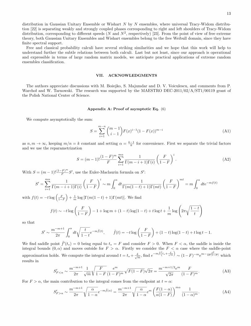
Appendix A: Proof of asymptotic Eq. (6)
We compute asymptotically the sum:
S =
m−n∑i=1
(m− 1
i− 1
)F (x)i−1(1− F (x))m−i (A1)
as n,m → ∞, keeping m/n = k constant and setting α = k−1k for convenience. First we separate the trivial factors
and we use the reparametrization
S = (m− 1)!(1− F )m
F
mα∑i=1
1
Γ(m− i+ 1)Γ(i)
(F
1− F
)i. (A2)
With S = (m− 1)! (1−F )m
F S′, use the Euler-Maclaurin formula on S′:
S′ =
mα∑i=1
1
Γ(m− i+ 1)Γ(i)
(F
1− F
)i∼ m
∫ α
0
dt1
Γ(m(1− t) + 1)Γ(mt)
(F
1− F
)mt= m
∫ α
0
dte−mf(t)
with f(t) = −t log(
F1−F
)+ 1
m log [Γ(m(1− t) + 1)Γ(mt)]. We find
f(t) ∼ −t log
(F
1− F
)− 1 + logm+ (1− t) log(1− t) + t log t+
1
mlog
(2π
√1− tt
)so that
S′ ∼ m−m+1
2π
∫ α
0
dt
√t
1− te−mf(t), f(t) = −t log
(F
1− F
)+ (1− t) log(1− t) + t log t− 1.
We find saddle point f ′(t∗) = 0 being equal to t∗ = F and consider F > 0. When F < α, the saddle is inside theintegral bounds (0, α) and moves outside for F > α. Firstly we consider the F < α case where the saddle-point
approximation holds. We compute the integral around t = t∗+ δ√m
, find e−mf
(t∗+
δ√m
)∼ (1−F )−mem−
δ2
2F (1−F ) which
results in
S′F<α ∼m−m+1
2π
1√m
√F
1− Fem
(1− F )m
√F (1− F )
√2π =
m−m+1/2em√2π
F
(1− F )m. (A3)
For F > α, the main contribution to the integral comes from the endpoint at t = α:
S′F>α ∼m−m+1
2π
√α
1− αe−mf(α) =
m−m+1
2π
√α
1− αem(F (1− α)
α(1− F )
)mα1
(1− α)m. (A4)
14
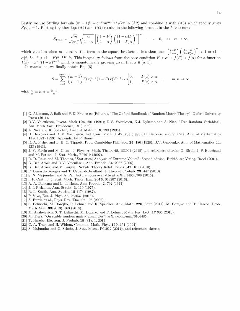
Lastly we use Stirling formula (m − 1)! ∼ e−mmm−1/2√2π in (A2) and combine it with (A3) which readily givesSF<α = 1. Putting together Eqs (A4) and (A2) results in the following formula in the F > α case:
SF>α ∼√m√
2πF
√α
1− α
[(1− F1− α
)((1− α)F
(1− F )α
)α]m−→ 0, as m→∞,
which vanishes when m → ∞ as the term in the square brackets is less than one:(
1−F1−α
)((1−α)F(1−F )α
)α< 1 or (1 −
α)α−1α−α < (1 − F )α−1F−α. This inequality follows from the base condition F > α → f(F ) > f(α) for a functionf(x) = x−α(1− x)α−1 which is monotonically growing given that x ∈ (α, 1).
In conclusion, we finally obtain Eq. (6):
S =
m−n∑i=1
(m− 1
i− 1
)F (x)i−1(1− F (x))m−i ∼
{0, F (x) > α
1, F (x) < α, m, n→∞,
with mn = k, α = k−1
k .
[1] G. Akemann, J. Baik and P. Di Francesco (Editors), ”The Oxford Handbook of Random Matrix Theory”, Oxford UniversityPress (2011).
[2] D.V. Voiculescu, Invent. Math 104, 201 (1991); D.V. Voiculescu, K.J. Dykema and A. Nica, ”Free Random Variables”,Am. Math. Soc., Providence, RI (1992).
[3] A. Nica and R. Speicher, Amer. J. Math. 118, 799 (1996).[4] H. Bercovici and D. V. Voiculescu, Ind. Univ. Math. J. 42, 733 (1993); H. Bercovici and V. Pata, Ann. of Mathematics
149, 1023 (1999), Appendix by P. Biane.[5] R. A. Fisher and L. H. C. Tippett, Proc. Cambridge Phil. Soc. 24, 180 (1928); B.V. Gnedenko, Ann. of Mathematics 44,
423 (1943).[6] J.-Y. Fortin and M. Clusel, J. Phys. A: Math. Theor. 48, 183001 (2015) and references therein; G. Biroli, J.-P. Bouchaud
and M. Potters, J. Stat. Mech., P07019 (2007).[7] R. D. Reiss and M. Thomas, ”Statistical Analysis of Extreme Values”, Second edition, Birkhauser Verlag, Basel (2001).[8] G. Ben Arous and D.V. Voiculescu, Ann. Probab. 34, 2037 (2006).[9] G. Ben Arous, and V. Kargin, Probab. Theory Relat. Fields 147, 161 (2010).
[10] F. Benaych-Georges and T. Cabanal-Duvillard, J. Theoret. Probab. 23, 447 (2010).[11] S. N. Majumdar, and A. Pal, lecture notes available at arXiv:1406.6768 (2015).[12] I. P. Castillo, J. Stat. Mech. Theor. Exp. 2016, 063207 (2016).[13] A. A. Balkema and L. de Haan, Ann. Probab. 2, 792 (1974).[14] J. I. Pickands, Ann. Statist. 3, 119 (1975).[15] R. L. Smith, Ann. Statist. 15 1174 (1987).[16] P. Vivo, Eur. J. Phys. 36, 055037 (2015).[17] Z. Burda et al., Phys. Rev. E65, 021106 (2002),[18] S. Belinschi, M. Bozejko, F. Lehner and R. Speicher, Adv. Math. 226, 3677 (2011); M. Bozejko and T. Hasebe, Prob.
Math. Stat. 33(2013), 363 (2013).[19] M. Anshelevich, S. T. Belinschi, M. Bozejko and F. Lehner, Math. Res. Lett. 17 905 (2010).[20] M. Tierz, ”On stable random matrix ensembles”, arXiv:cond-mat/0106485.[21] T. Hasebe, Electron. J. Probab. 19 (81), 1, 2014.[22] C. A. Tracy and H. Widom, Commun. Math. Phys. 159, 151 (1994).[23] S. Majumdar and G. Schehr, J. Stat. Mech., P01012 (2014), and references therein.