Embed Size (px)
Citation preview

Document de travail IDP (EA 1384) n°2013-13
Pecking order versus trade off theory and the issue of debt
constraint problem?
Mohamed Ramdani et Ludovic Vigneron
RIO – Risque, Information, Obligation

Pecking order versus trade off theory and the issue
of debt constraint problem?
Mohamed Ramdani et Ludovic Vigneron
Mohamed Ramdani
PRES Université Lille Nord de France, Université de Valenciennes et du Hainaut-
Cambrésis, IDP, EA1384, Valenciennes, France
Ludovic Vigneron
PRES Université Lille Nord de France, Université de Valenciennes et du Hainaut-
Cambrésis, IDP, EA1384, Valenciennes, France

1
“Pecking order versus trade off theory and
the issue of debt constraint problem?”
Mohamed Ramdani
Maître de Conférences
Université de Lille Nord de France - IDP
Institut du Développement et de la Prospective
Ludovic Vigneron1
Maître de Conférences
Université de Lille Nord de France - IDP
Institut du Développement et de la Prospective
Abstract:
This paper presents a new test investigating competing capital structure theories. Our test was
performed more particularly on a sample of French quoted firms. The question is which one
of pecking order or trade off theory can be considered as a better first order explanation for
firms’ behaviors. This test seeks to shed some new light on the issue of debt constraint
problem and its effects. We use both linear and un-linear specifications of the relationship
between the firm’s debt variation and financial deficit to deal with this difficulty. In the
classical linear context, our findings show that trade off theory dominates pecking order for
constrained firms whereas pecking order dominates trade off theory for unconstrained ones.
However, we will show the introduction of that un-linear specifications improves pecking
order adjustment and makes it difficult to distinguish which theory better fits.
Key words: Capital structure, Trade off theory, Pecking order theory, debt constraint
JEL classification: G32
1 Contact : [email protected]
2
INTRODUCTION
Financial structure puzzle is one of the oldest and more prolific research topics in corporate
finance. Since Modigliani and Miller (1958, 1963) seminal papers, many other articles have
dealt with the issue of firms’debt rational choice. Current debates focus on whether trade-off
or pecking order theory better explains companies’ behaviors. Shyam-Sunder and Myers
(1999) proposed a test to arbitrate between these two analyses and concluded in favor of
pecking order. But their results were contested by Chirinko and Singha (2000) and Frank and
Goyal (2003). One of the most important addressed criticisms is that their empirical evidence
did not perfectly reflect pecking order financing. Lemmon and Zender (2010) stated that this
relatively poor performance of Shyam-Sunder and Myers’ test could be explained through of
firms’ limited debt capacity and proposed a modified test to deal with this issue. They
considered an un-linear relationship between debt variation and need for external finance.
The new test we develop in this paper seeks to contribute to the pecking order versus trade off
debate. It considers the impact of difficulties that firms can face if they want to finance
important needs (or if they want to use the important excess in their internal resources) on
discriminatory power of previous test. We examine the question of which one these two
theories is a better first order explanation of firms’ financial behaviors considering debt
constraint problem. Our investigation was conducted in a different institutional context than
previous studies used to consider. More specifically a new dataset of French firms provided
different results from the previous studies which were mostly conducted in an Anglo-Saxon
context. Through the example of France and its economy based on a bank-centered financial
system, our data have allowed us to present original results. In our sample, pecking order
behavior must be more relevant because of difficulties in issuing equities in the French capital
market.
To start our analysis, we first replicate classical versions of pecking order theory tests by
financial deficit and trade off theory test by target adjustment through mean reversion. These
two dependent variables have a significant impact on the variations of the debt of firms. Then,
we consider differences in debt financial behaviors for constrained and unconstrained firms.
We clearly observe that access to debt is an important dimension to be considered especially
when the question of capital structure puzzle is at stake and when you consider pecking order
theory tests. For classical linear specifications of financial deficit, we document that, in the
case of debt constrained firms, target adjustment is a better first order explanation of debt

3
variation than financial deficit and, for unconstrained ones, we document that financial deficit
appears to be a better first order explanation for debt variation. For un-linear specifications,
more exploration is needed. Indeed, the relationship between financial deficit and debt
variations become more important and we can’t distinguish whether pecking order or trade off
theory is a better first order explanation for capital structure.
This article is organized as follows. Section one quickly discusses the literature about
financial structure and focuses on prior tests and develops our hypotheses. Section two
describes the dataset and specifications of our tests. Section three presents our main results we
obtained after we performed some robustness checks tests.
I. LITERATURE AND HYPOTHESES
A. LITERATURE
On perfect market contexts, the capital structure issue is irrelevant (Modigliani and Miller,
1958). The firms’ financing choice is only a question of cash flow allocation and it does not
influence the project choice or firm value. Modern financial theory goes beyond this
simplified analytical context. Two dominant classes of models are currently employed to
explain capital structure: trade-off and pecking order. Empirical researches continuously fuel
approaches without conclusive answers in favor of one or the other because they are not
mutually exclusive and do not fully explain firms’ behavior2.
For trade-off theory, firm capital structure choice results from an arbitrage between costs and
debt benefits. The most important explaining factors used in literature are tax reduction and
increases in bankruptcy costs. Bradley et al. (1984) present a static version of this class of
model in which firms choose optimal financial leverage balancing debt and equity finance to
maximize their value. They consider different tax rates for investors who buy bonds or
equities. They show that optimal debt level increases with both tax rate on equities and costs
of distress but decreases with tax rate on bonds. The main problem of these static models is
that they predict only one optimal solution that the firm must always met. This is not realistic.
For example, there are no retained earnings. This imperfect model requires the necessity to
use a new class of models, such as dynamic trade-off models in which the financing decision
2 For a more exhaustive review see Franck and Goyal (2007)

4
depends on the financing margin anticipated by the firm. These models include retained
earnings as internal equities and focus on the fact that the money which stay in the firm is not
taxed but the money paid out is taxed (Stiglitz, 1973). Following this approach, Kane et al.
(1984), Brennan and Schwartz (1984) show that firms rebalance their leverage to adapt
themselves after shocks and to converge to optimal structures. Fischer et al. (1989) introduce
transaction costs in the dynamic trade-off to obtain a more realistic rebalancing behavior. In
this context, convergence to optimal capital structure can be slower.
As regards, pecking order theory, there is not necessarily an optimal capital structure but a
hierarchy between different sources of funds which try to minimize asymmetric information
problems. Firms prefer internal to external financing and debt to equity. They first employ all
their retained earnings and then they use debt. Equities are issued after the firms’ debt
capacity is reached. Myers and Majluf (1984) are at the origin of this class of models. They
consider an adverse selection problem which leads good firms to prefer internal financing to
fund their positive net present value projects, because external investors will charge them at
the same level as bad firms. In this context, the cost of external equity can lead good firms to
give up profitable opportunities. External debts are not explicitly included in the analysis but,
as Myers (1984) notes, lenders priority over firm’s cash flow make debt less risky than equity
and so cheaper. Myers (2003) proposes a version of pecking order based on agency costs.
Managers always prefer internal financing because outside financing exposes them to
monitoring which reduces their perk consumption. If it is not enough, external equity issue is
not an inefficient solution because it leads to underinvestment. Managers limit profitable
projects they can undertake to preserve their perk consumption. External debt is a better
solution because of fix cash flow associate with which can discipline managers.
The main tests of current theories currently focus on two empirical strategies: target
adjustment of companies’ leverage for trade-off theories and debt funding of financial deficit
for pecking order theories.
The first strategy is the oldest approach (Taggart, 1977). It postulates that, because of random
exogenous shocks in their access to the different sources of funds, the capital structure of
firms may be different from the optimal structure, but they sequentially correct this fact by
issuing or buying back debts or equities to converge to the optimal structure. The tests consist
in two sequences. The first sequence consists in checking if the leverage ratio is effectively
adjusted to reach a target and the second one in measuring the speed of this adjustment. The

5
main difficulty here is to estimate optimal leverage. The most classic way to proceed is to use
the historical means of leverage as a proxy (Marsh, 1982; Jalilvand and Harris, 1984; Fama
and French, 2001). This method implicitly supposes that the firms’ characteristics which
influence optimal capital structure are relatively stable over time. More recently, more
sophisticated estimations for target leverage have been developed. Hovakimian et al. (2001)
use a two-stage method. In a first step, they use regression leverage over the firms’
characteristics and in a second step, they use obtained estimations minus the firm’s actual
leverage with control factors in a logit regression of financing choice of firm. Kotrajczyk and
levy (2003), Kayhan and Titman (2007) use the same kind of method. The main results of
these studies are that firms adjust their leverage to a target. The leverage in question is mean
reverting, but this move toward optimal ratio is relatively slow (Fama and French, 2002). In a
study about the United Kingdom and continual Europe, Wanzenried (2006) documents that
the speed of adjustment depends on the institutional context.
The second strategy was originally elaborated by Shyam-Sunder and Myers (1999). The
starting point is that in pecking order context, every need for external funds must be fulfilled
with debts because debts are cheaper than equities. So we must document a strictly
proportional link between the need for external funds, the firms’ financial deficit, and the
debts variation. When firms have a positive financial deficit, they must issue debts, and when
they have a negative one, they must pay back their debts. Unfortunately, studies based on this
method fail to find perfect correlation between changes in debt and financial deficit but they
document all the same evidences of a strong one. In France, we can refer to Aktas et al.
(2011) for very small business, or to Molay (2005) for big firms. Shyam-Sunder and Myers
(1999) compare these findings with the classical target adjustment method and conclude that
pecking order theory is more efficient to predict a firm’s behavior than trade-off theory. Frank
and Goyal (2003) contest this interpretation. They show over a larger and longer dataset that
the relations between debt variations and financial deficit depend on the period and the
category of the firms. They point at two paradoxical results which contradict pecking order
predictions. First, young and rapidly growing firms, for which adverse selection problems are
important, finance most of their needs by equities. Second, big and mature firms, for which
adverse selection problems are low, mostly rely on debts to finance their needs. Globally, in
line with Fama and French (2005), the authors document that too many issues of equities are
not launched at an appropriate time to support pecking order theory.

6
Chirinko and Singha (2000) propose a critical analysis of these two strategies. They point that
both test pecking order test by financial deficit and tradeoff test by target adjustment - are
misleading because their results can be explained by other factors. One of them is credit
constraint (Leary and Roberts, 2010). Lemmon and Zender (2010) address the problem and
offer a new test for pecking order theory. They modify Shyam-Sunder and Myers test by
using a quadratic specification for financial deficit. Their point is that if firms are constrained
in issuing debts, they cannot borrow more after a certain amount. So the link between
financial deficit and debt variation must be important before this limit and marginally small
after. In this context, they estimate that it is easier for companies to finance a small financial
deficit than a big one because of limited debt capacity. They offer evidence in line with this
hypothesis documenting that quadratic specifications significantly improve inference for
credit constrained firms and have no effect for unconstrained ones.
B. HYPOTHESES
Following Shyam-Sunder and Myers (1999), we have been conducting an analysis with the
two previously described empirical strategies. Our purpose is to test which theory, pecking
order or trade-off, is a better first order explanation for firm’s capital structure choice
considering the firm’s debt constraints.
Our starting point is the classic pecking order test based on financial deficit. Previous studies
document mixed results about the link between debt variation and financial deficit. The initial
hypothesis of a perfect correlation fails to fit the facts. Coefficients of regression documented
in literature are always smaller than 1. These results show that firms partially finance their
financial deficit with new equities. Taking into account these facts, following Aktas et al.
(2011), we consider a less restrictive hypothesis than the initial test. We only expect a positive
correlation between the firms’ debt variations and their financial deficit (hypothesis 1).
According to Leary and Robert (2010) and Lemmon and Zender (2010), the poor performance
of classic pecking order test is attributed to the firms’ debt constraints. Two causes can
explain the constraints. First, as Myers (1977) points out, firms can have so many debts that
every increase in debt reduces the total market value of their debt. Because of more probable
distress and implied costs, potential lenders will charge a higher rate which makes debts as
expensive as equities. Firms have issued too many debts in the past and they have reached the
limit. Second, as point Stiglitz and Weiss (1981), lenders can ration debt because of

7
asymmetric information problems. Because of adverse selection problems or anticipated
moral hazard problems, debt suppliers limit their lending to firms for which it is hard to assess
real risk. In this context, even good firms, those with low real risks, can be constrained for
their debt issuance because lenders cannot distinguish them from bad firms, those with high
real risks. The Equities issues subscribed by the CEO (Leland and Pile, 1977) and collateral
(Bester, 1987) can be used to mitigate these difficulties. Considering that it could be hard for
firms to issue debts, we expect that the link between the firms’ debt variations and their
financial deficit will be more important for unconstrained firms than for constrained ones
(hypothesis 2).
Previous empirical research documents disturbing results in pecking order theory point of
view for both young rapidly growing firms and large mature ones. Young rapidly growing
firms rely mostly on equities to finance their financial deficit and large mature firms on debts
(Frank and Goyal, 2003). Two opposite explanations are given. Halov and Heider (2011)
argue that the classic interpretation of debt in pecking order theory is misleading. Because of
asymmetric information problems, debts can be mispriced and finally more costly than
equities. In this context, more opaque firms, such as young and rapidly growing ones, prefer
equities to debts and mature ones prefer debts to equities. Lemmon and Zender (2010)
attribute these counter intuitive results to the firms’ debt constraints. Young firms face an
important mortality rate and have few tangible assets to offer as a warranty to debt suppliers.
These firms have no way to distinguish themselves if they are less risky. In this context,
young firms can quickly reach their limit debt ratio. Mature firms do not have to deal with this
kind of problems. To cope with the firm’s debt constraints in the pecking order test, Lemmon
and Zender (2010) use the quadratic specification for the relationship between debt variation
and financial deficit. The idea is that for debt constrained firms, a big deficit must be harder to
finance than a small one. Following this approach, we expect that the use of an un-linear
specification for financial deficit improves the inference quality of classic pecking order
behavior for firms suffering from debt constraints (hypothesis 3).
Our second point is the test for trade off theory through target adjustment. We use a mean
reverting process to model firms’ behavior. As in Shyam-Sunder and Myer (1999) or in Frank
and Goyal (2003), we estimate the target with the historical mean of debt ratio. Trade off
theory predicts that firms issue or pay back debts to meet their optimal debt ratio. This latter
maximizes the firm’s value by taking into account distress costs, taxes reduction associated

8
with debts and reduction of agency costs. This behavior is not affected by debt constraint
because if firms cannot adjust their ratio through debt variation, they can do it by variation of
equities. Previous studies find evidence of positive correlations between debt variations and
mean reverting factor even if, as for financial deficit in the pecking order theory, this
correlation appears relatively small. Fischer et al. (1989) attribute this fact to the cost of
transactions associated with adjustments. According to these elements, we expect a positive
correlation between debt variation and the mean reverting factor of debt ratio (hypothesis 4).
This correlation will not be different for debts of constrained and unconstrained firms
(hypothesis 5).
As previously discussed, the question of which theory, pecking order or trade off theory, can
be a better explain the firm’s capital structure, have not been answered yet. One difficulty is
that they are not mutually exclusive (Graham and Leary, 2011). Results of joint tests, tests on
the firm’s debt variations, including both financial deficit and target adjustment, depend on
the sample selection and the period during which they are performed (Frank and Goyal,
2003). Even if robustness of conclusion can be discussed, some regularity has been
documented. For example Psillaki and Daskalis (2009) show that determinants of capital
structure do not differ across countries in which a civil law system is prominent. Their study
focuses on four European countries including France. This particular context seems to be
favorable for the pecking order behavior. Even if we focus on big quoted firms, less
developed equity markets than US ones and bank centered financial system, limit possibilities
to issue external equities. So financial deficit is expected to be a better first order determinant
of debt variations than target adjustment (hypothesis 6).
II. DATA AND METHODOLOGY
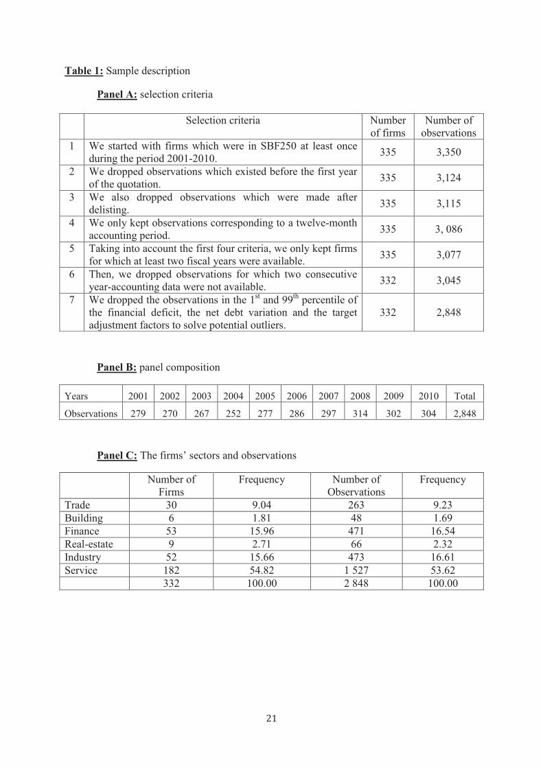
A. SAMPLE DESCRIPTION:
In order to conduct our investigation, we used a sample of 335 firms which were part of SBF
2503 at least once during the period 2001-2010. This choice has allowed us to work with a
sufficiently large number of firms which present differences in size and age and for which
information is easily available. Our data were extracted from both DIANE4 database, for
3 This index is composed by the 250 biggest market capitalizations trade in Paris stock exchange its base is
one thousand the 28th December 1990. 4 DIANE is edited by Bureau Van Dijk (92, rue de Richelieu 75002 PARIS)

9
accounting data, and Europe Daily5 database, for market ones. We did not consider
observations before Initial Public Offering (IPO) and after delisting. Mistakes and gaps in
data were either directly corrected with the information provided by alternative sources like
companies’ reports when it was possible or there were dropped when no data could be found.
Finally, we only kept the firms for which the financial statement for at least a two-year
consecutive twelve-month accounting period has available. From this preliminary database,
we computed the firms’ financial deficit, the net debt variation debt and the mean reversion of
financial leverage. Then we deleted the observations part of the 1st and the 99
th percentile of
these variables to solve the potential outlier problems. Table 1 offers details about our
sampling procedure and the main characteristics of the resulting sample. We have an
unbalanced panel with gaps. It includes 332 firms providing a total of 2,848 observations.
About 55% percent of these firms operate in the service sector, 16% in the finance sector and
15.5% in the industry sector.
In table 2, we present some descriptive statistics computed for our sample. Some points have
to be discussed before going further. First, we note an important heterogeneity between the
companies’ sizes and ages of the companies. We both have very old big firms and young
quoted small and medium-sized companies. The differences in total asset6 and market
capitalization are huge across the sample. Second, the proportion of tangible assets in total
assets is relatively low for the firms of our sample, a mean ratio of 5%. Two reasons explain
this low level: most of them belong to big groups with important long-term investments
and/or operate in the service sector. Third, the firms’ operating performance is also relatively
low with a mean return on assets (ROA) of -2.7% over the total period. About a third of the
observed, ROAs is negative. This proportion was more important after the beginning of the
financial crisis in 2007. Thirty-four percent of firms reported a negative operating income
after the crisis against 30% before. Fourth, statistics on total leverage and financial leverage
ratios indicate that total liabilities are composed on average for 47.9% of debts and 36.7% of
financial debts. These values are in line with 42% (without reprocessing) of the total leverage
documented by Molay (2005) over the first Paris market between 1995 and 2002. Aktas et al.
(2011), who worked on French very small businesses between 1998 and 2006, documented a
more important total leverage of 52% and a lower financial leverage of 20%. They attributed
5 Europe Daily is edited by EUROFIDAI and distributed by IODS (48, rue de Provence 75009 PARIS). 6 Every accounting data used in the study is reprocessed to provide a more informative content. We have
cancelled subscribed but not called stock, preliminary expenses, subscribed-called but not paid stock,
premium bonds. We have re-entered leasing and discounted bills.

10
the relatively high value of the total leverage to limited access to the primary equity market
and to the absence of the secondary market. Equities are mainly held by the owner’s family.
They explain the low financial leverage through credit rationing. The main external source of
debt for small firms is the trade credit offered by their suppliers. Fifth, in our sample, the
firm’s main source of debt is what we call other borrowing. It includes the partners’ current
accounts, the employee profit-sharing and so on. We qualify this form of debt as internal
debts. The second most important source of debt and the first external one are bank loans
which account for 25.2% of total debts. The second and third external source of debt is trade
credit, 18.2%. Bond issues are relatively small and only represent an average of 9.6% in total
debts. Most of the companies do not use the market debt. The median ratio of bond in debts is
0. Financial leasing is seldomly used. On average, this form of financing is inferior to 1%.
During the total period, less than half of our sample had had an ongoing contract.
B. METHODOLOGY:
In this subsection, we present our econometric models and briefly discus variables included in
the specifications. We provide summary statistics and synthetic definitions for those different
variables in table 2 and appendices 1 and 2. We test the hypothesis presented in section 2 on
our sample of 332 French quoted firms. Our methodology is inspired from the two step
procedure used by Lemmon and Zender (2010). In the first step, we build a proxy of debt
constraint and we use it to split our dataset in three groups using terciles. Then we have highly
constrained, moderately constrained and less constrained firms. In the second step, we run our
regressions inspired from Shyam-Sunder and Myer (1999) over the two extreme groups to
compare inference about our different specifications between the subsamples of the most and
least constrained firms.
In order to measure the debt constraint, we estimate the probability for a firm to issue public
debts as a function of its characteristics. Using this proxy, we follow the theoretical analysis
provided by Bolton and Freixas (2000). They show that the safest firms, those which can
borrow more easily because of their low probability of distress, prefer to issue public debt to
avoid cost of intermediation incurred with bank debt. Riskier firms borrow only from banks to
benefit from flexibility provided by these financial intermediaries. Holstrom and Tirole
(1997) reach the same conclusion. Lemmon and Zender (2010), following Almeida, Campello
and Weisbach (2004) and others, use the existence of a bond rating as proxy of public debt
use. We opt for a more direct measure. This choice is in line with Faulkender and Petersen

11
(2006) who asked whether the use of finance sources affected the capital structure choice. Our
method allows us to examine if access to bond market affects pecking order or target
adjustment behaviors. We use accounting data to infer if a firm has issued a new public debt
or not. We code a dummy variable whose value is 1 if the firm’s total outstanding public debt
increased between a period of two years and we use it as a dependent variable in a probit
regression over the firms’ characteristics. The explanatory variables are the firm’s size (ln
total assets), profitability (ROA), assets tangibility, leverage, age (ln age), risk (standard
deviation of stocks returns) and industry dummy variables (NAF2 Rev. 2 digit or big
sectors7). All variables are lagged for period 1. These variables are the same as those used by
Faulkender and Petersen (2006). Table 3 provides estimation results for three different
specifications in which we control or not for industrial sectors. We use predictions associate
with the first model to split our sample.
We performed the main tests over the entire sample, over the most constrained firms and the
least constrained firms. These tests are built on the same basis. We used regression to estimate
the variations of the net financial debt between two consecutive years over pecking order
and/or trade off factors. Contrary to other comparable studies, we opted for the net financial
debt which is computed by taking the total of the financial debts minus the firm’s treasury
assets. This choice allowed us to control the effect of the use of the treasury variations
required to the firm’s financial needs. All our estimations considered both the year and the
firm’s fixed-effects so that constant over time and over firm omitted variables were taken into
account.
To test hypothesis 1, we adopted the following econometric specification:
(1)
Where is the variation of net debts for the firm i over the t t-1 period, represents
the year fixed-effect, represents the firm’s fixed-effect and is the financial
deficit for the firm i over the t t-1. This last variable measures the needs for external funds.
We computed it as the sum of dividends paid plus the net investment expense plus the change
in working capital minus the operational cash flow after interests and taxes. Both variations of
net debts and financial deficit are standardized by total economic assets8 in t-1. We
extensively described the mechanism of this test in appendix 2. To test hypothesis 2, we run
7 Commerce, Construction, Finance, Real estate, Manufacturing, Service. 8 Net fixed assets plus working capital.

12
regression over subsamples of the most constrained or the least constrained firms and
compared . To test hypothesis 3, we introduced the square of in the regression
equation. A positive coefficient associated with the classic variable and a negative one
associated with the squared variable indicated that the debt variation increased with the
financial deficit up to a certain deficit level and after it increased more slowly.
To test hypothesis 4, in which we focus on the target adjustment process, we adopted the
following specifications:
(2)
Where is the target financial leverage ratio that we estimate by the average financial ratio
over the entire period of study and where is the financial leverage ratio in t-1,
represents the target adjustment factor. To test hypothesis 5, we run the regression
over the most constrainted and the least constrained firms and compared the results.
To test hypothesis 6, we adopted the following specifications:
(3)
We included both financial deficit and target adjustment factors in the regression equation.
This allowed us to compare pecking order and trade off theory as a first order explanation for
a firm’s variation when taking into account financial debts having an impact on debt
constraints.
In addition, in order to consider the potential effects of the debt constraint, we modified the
specifications.
(4)
We also added the squared of the financial deficit in the current equation.
III. RESULTS:
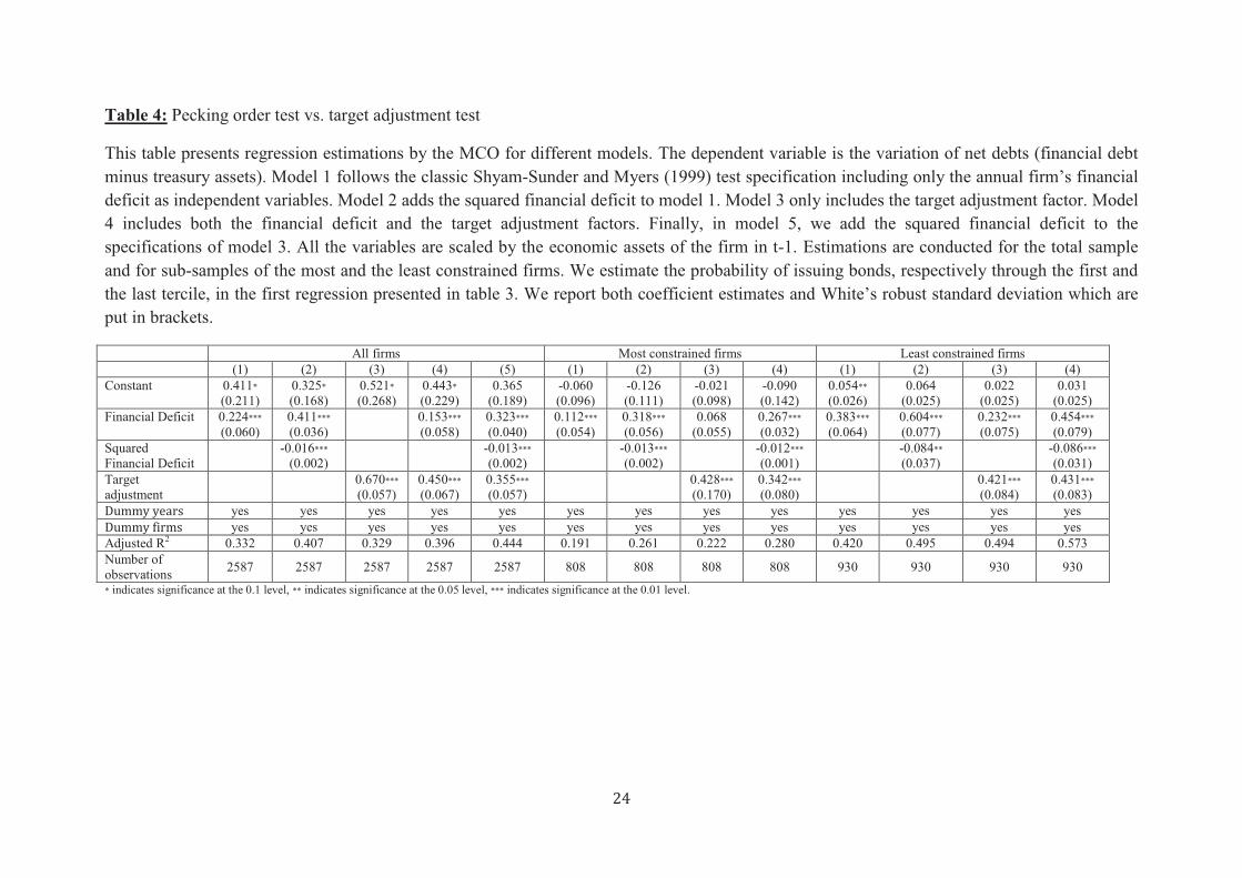
A. MAIN RESULTS:
Table 4 reports the results for the tests of our different hypotheses. In the first column, we
present the classic Shyam-Sunder and Myer (1999) test performed on variation of net debt for

13
the total sample. The coefficient associated with the financial deficit is 0.224. It is relatively
low but positive and significant, which is in line with our hypothesis 1. Previous studies
reported higher values but they did not correct for treasury variation. In the US context,
Shyam-Sunder and Myer (1999) documented a value of 0.79. Frank and Goyal (2003), who
performed the same test over a longer period in the US, globally documented 0.748, but only
0.33 after 1990. They concluded that pecking order had a decreasing explanatory power for
more recent years. Our results are close to them. For very small businesses in the French
context, Aktas et al. (2011) documented a coefficient of 0.79. This value was even more
important for the firms which had a positive deficit. We attribute the difference with our
findings mainly to difficulties that very small businesses encounter to issue equities compared
with quoted firms. A previous study, performed by Molay (2005) between 1995 and 2002,
documented a coefficient of 0.41 for quoted firms.
Relatively low values of pecking order adjustment, in our first regression, can be associated
with the firm’s debt constraints. Our estimates of the same model on sub-samples of the most
constrained and the least constrained firms are in line with this statement. We report a
coefficient of 0.112 with a relatively low adjusted R2 (0.191) for the first group and 0.383
with a higher adjusted R2 (0.420) for the second one. This difference is significant at the level
of 0.05. The value of the t of the Student, for the mean comparison test that we performed, is
2.296. This result is in agreement with the prediction formulated in hypothesis 2.
In the second column of the table, we use the Lemmon and Zender (2010) test for the entire
sample. The introduction of the squared financial deficit strongly improves the pecking order
adjustment. The coefficient associated with the linear specification is 0.224. In the un-linear
one, it is almost twice as high (0.411) and the coefficient associated with the squared term is
negative (-0.016) and significant. The adjusted R2 of the model also increased significantly. It
increased from 0.332 to 0.407. Even if difficulties to finance big deficits affect constrained
and unconstrained firms, the coefficient associated with the squared term is negative and
significant in both cases, for the most constrained firms, the un-linear transformation has an
more important impact on inference quality. The coefficient associated with the financial
deficit has almost tripled and the adjusted R2 has increased by a 7-point basis. For the least
constrained firms, the coefficient has only doubled and adjusted R2 has also increased also
about 7 basis points. This difference appears to be consistent with our hypothesis 3.

14
The test for our hypothesis 4 is presented in the third column of the table. The coefficient
associated with the target adjustment by mean reverting, 0.67, is positive and significant as
we expected. Its relatively low value, less than one, is generally attributed to the adjustment
cost. When we include this new factor in the previous regression equation, we document both
a lower coefficient for the target adjustment and for the financial deficit. The link between the
net debt variation and the new factor, which can be interpreted as the speed of adjustment to
optimal capital structure, is almost the same if we compare constrained and unconstrained
firms in both linear and un linear specifications of pecking order adjustment. The difference
between the coefficients for the two groups is not significantly different from 0. This report is
consistent with our hypothesis 5.
For our hypothesis 6, the most important one, we examine values of coefficients associated
with the financial deficit and target adjustment to determine which of pecking order theory or
trade off theory is the better first order explanation for a firm’s net debt variation. In the linear
specification regression, the target adjustment clearly appears to be the main factor with a
coefficient of 0.45 against 0.153 for the financial deficit in the total sample analysis. This
difference is even more important for the sub-sample of most constrained firms for which the
introduction of target adjustment makes the coefficient associated with the financial deficit is
not significantly different from 0. The results for least constrained firms are close to those
discussed on the total sample (0.421 against 0.232). In the un-linear specification regressions,
differences between pecking order and trade-off theory are not significant, and those on the
total sample as well as on each sub-sample. The introduction of a squared financial deficit,
aiming at controlling growing difficulties to deal with the biggest deficit, improve the
explanatory power of pecking order theory. This makes the question of which the theory
prevails. In each of our estimation, on sub-groups and on the total sample, we cannot tell
which theory prevails with any certainty. is not significantly different from in
quadratic context. So, we do not validate our last hypothesis.
B. ADDITIONAL RESULTS AND ROBUSTNESS CHECK TESTS:
In this section, we examine whether the results are robust for alternative measures of debt
constraints. We consider two categories of alternative ways to split the sample to distinguish
potentially most and less constraint firms. First, we consider the fact that firms issue or not
bonds instead of estimation then probability of doing it. Secondly, following Hadlock and
Pierce (2010) who recommended using the firms’ ages and sizes as proxies for financial

15
constraints, we split the sample on tercile for these two variables. Then, we oppose the
smallest firms in terms of total assets to the biggest ones in a first step, and the youngest ones
to oldest ones in a second step.
By computing the yearly firms’ probability to issue bonds with the view to assessing their
access to external financial debts, we consider both the firms that effectively follow this
framework and those whose characteristics allow them to do so bur do not. The procedure
gives us the possibility to work with more important groups of firms considered as debt
constrained or not. In table 5, we present alternative results associated with a more restrictive
approach to bond issues. We did not reproduce each test performed in table 4 but only the
most important ones. We provide new estimations for equations 1, 2 and 4. The first part of
the table presents the sample decomposition between the firms which issued bonds between
2001 and 2010 and those which did not. The second part presents the decomposition between
the firms that issued bonds at least once during the period of the study and those which did
not. Each time, we opposed the least debt-constrained firms to the most debt-constrained
ones. Results are globally consistent with conclusions provided by the analysis of the main
tests. The financial deficit and target adjustment factors are positive and significant. The
inclusion of a squared financial deficit in the regression improves the pecking order
adjustment for the most constrained firms but have no significant effect for the least
constrained ones. The financial deficit and target adjustment appear to have no significantly
different explanatory powers on variation of net financial debt for the least constrained firms
and for the most constrainted ones in un-linear specifications.
In the second robustness check tests, instead of focusing on the type of the debts firms issue in
order to assess their potential debt constraints, we used the firms’ sizes and ages to split our
sample. The smallest and the youngest firms are reputed to have a more limited access to
external finance than the biggest and oldest ones. As in the main tests, we compared extreme
terciles to document behavioral differences in terms of financial net debt variations. We
performed the same regressions as those in table 5. Estimation results are presented in table 6.
The sub-sample change slightly affects coefficients for pecking order and trade - off theory.
The conclusions about our different hypotheses are globally the same. If we want to explain a
firm’s capital structure evolution, we notice that the financial deficit and the target adjustment
are both positive and have significant factors. However, we cannot distinguish which one is a
better first order explanatory factor for the smallest and youngest firms, in the un-linear
specification. The only exception is for the biggest and oldest firms when we include a
16
squared financial deficit. We report a significant difference between the pecking order
adjustment and trade off theory. The first one appears to be more important than the second
one. In this particular context, the results we have found are consistent with our hypothesis 6.
Pecking order is a better first order determinant for big and old firms when you consider that
it is more difficult to finance a big financial deficit than a small one.
IV. CONCLUSION:
In this article, we have examined the question of whether pecking order or trade-off theory is
a better first order explanation for a firm’s capital structure choice. Previous tests, following
Shyam-Sunder and Myers (1999) methodology, produce mixt results (Frank and Goyal,
2003). These difficulties are attributed to the failure of tests based on financial deficit to
consider the impact of firms’ limited debt capacity (Leary and Roberts, 2010). Lemmon and
Zender (2010) provide a modified version of these tests of pecking order theory based on an
un-linear specification of the relationship between financial deficit and debt variation. In
doing so, they consider difficulties for debt-constrained firms to finance the biggest financial
deficits. We have adapted this framework to consider both pecking order and trade off theory
adjustment to firms’ behaviors. We have confronted the explanatory power of debt financial
deficit and target adjustment by taking into account the firms’ debt constraint problem using
an un-linear specification.
We have found evidence that both pecking order and trade off theory are relevant to explain
the firms’ debt variation. Considering the debt constraint problem through many proxies, we
have shown that the access to credit has a significant impact on the way that firms finance
their external needs of funds but has virtually no effect on speed in which they adjust their
capital structure. The tests performed on un-linear specifications of financial deficit clearly
show that it is more difficult for a firm to finance bigger deficits than smaller ones. This
phenomenon appears more important for firms identified as more likely to be debt-
constrained. In a linear context, a first set of tests showed that trade off theory better fits the
data than pecking order theory for debt-constrained firms whereas a second set of tests
demonstrated that pecking order theory better fits the data than trade off theory for
unconstrained ones. However, the introduction of un-linear specifications makes it hard to
distinguish which theory is a better first order explanation for the choice of the firms’ capital
structure.

17
This last result leaves the question unanswered. Other investigations have to be conducted to
reach a better understanding of the firms’ financial structure and debts. Alternative theories
have to be considered and evaluated relatively to pecking order and trade-off theories. Market
timing theory is one of those. It postulates that firms do not seek to reach an optimal capital
structure or do not seek to issue debts or equities to minimize their adverse selection
problems. Firms finance themselves according to the opportunities offered in the market
(Baker and Wurgler, 2002). Firms issue debts or equities when these financing means are
widely available at a good price. A much more recent study advocates a model of life patterns
in firmrs’financing choice (La Rocca et al. 2011). Firms start to rely on debts at the first stage
of their life-cycle and gradually, when they reach a more mature stage, substitute internal
capitals to debts. Kayhana and Titman (2007) provide evidences that the firms’ capital
structure depends on their history even if, over the long term, they tend to adjust their debts to
their target structure. Behavioral finance also investigates the field. Heaton (2002), Ayres de
Barros and Di Miceli da Silviera (2008) document that overconfident and optimistic managers
tend to use more often debts. The main difficulty to deal with these different theories of
capital structure is that they are not mutually exclusive. The problem is to find a hierarchy
between them and not to reject or accept one or another.

18
Bibliography:
· Aktas N., Bellettre I. and Cousin J.G., 2011, “Capital structure decision of French very
small businesses”, Finance, 32, 43-73.
· Ayeres D. de C. Barros and Di Miceli da Silvieira, 2008, “Overconfidence, managerial
optimism and the determinants of capital structure”, European Financial Management
Conference, Athen.
· Baker M. and Wurgler J., 2002, “Market timing and capital structure”, Journal of
Finance, 57, 1-30.
· Bester H., 1987, “The role of collateral in credit markets with imperfect information”,
European Economic Review, 31, 887-899.
· Bolton P. and Freixas X., 2000, “Equity, bonds and bank debt: capital structure and
financial market equilibrium under asymmetric information”, Journal of Political
Economy, 108, 324-351.
· Bradley M., Jarrell G. and E.H. Kim, 1984, “On the existence of an optimal capital
structure: theory and evidence”, Journal of Finance 39, 857-877.
· Brennan M.J. and Schwartz E., 1984, “Optimal financial policy and firm valuation”,
Journal of Finance 39, 593-607.
· Chirinko R.S. and Singha A.P., 2000, “Testing static tradeoff against pecking order
models of capital structure: a critical comment”, Journal of Financial Economics 58,
417-425.
· Fama E. and French K., 2005, “Financing decisions: Who issues stock?”, Journal of
Financial Economics, 76, 549-582.
· Fama E.F. and French K.R., 2001, “Disappearing dividends: changing firm
characteristics or lower propensity to par?”, Journal of Financial Economics, 60, 3-43.
· Fama E.F. and French K.R., 2002, “Testing the tradeoff and pecking order predictions
about dividends and debt”, Review of Financial Studies, 15, 1-33.
· Faulkender M. and Petersen M. A., 2006, “Does the source of capital affect capital
structure?”, Review of Financial Studies, 19, 45–79.
· Fischer E., Heinkel R. and Zechner J., 1989, “Dynamic capital structure choice: theory
and tests”, Journal of Finance 44, 19-40.
· Franck M. and Goyal V., 2007, “Trade off and pecking order theory of debt”, ed.
Eckbo E., Handbook of Corporate Finance: Empirical Corporate Finance, 1-82.
· Frank M. and Goyal V., 2003, “Testing the pecking order theory of capital structure”,
Journal of Financial Economics, 67, 217-248.
· Graham J. and Leary M., 2011, “A review of empirical capital structure research and
directions for the future”, Annual review of Finance, 3, 309-345.
· Hadlock C.J. and Pierce J.R., 2010, “New evidence on measuring financial
constraints: moving beyond the KZ index”, Review of Financial Studies, 213, 1909-
1940.
· Heaton J., 2002, “Managerial optimism and corporate finance”, Financial
Management, 31, 33-45.

19
· Halov N. and Heider F., 2005, “Capital structure, risk and asymmetric information”,
Quarterly Journal of Finance, 1, 767-809.
· Holstrom B. and Tirole J., 1997, “Financial intermadiation, loanable funds, and real
sector”, Quarterly Journal of Economics, 112, 663-691.
· Hovakimian A., Opler T. and Titman, 2001, “The debt-equity choice”, Journal of
Financial and Quantitative Analysis, 36, 1-24.
· Jalilvand A. and Harris R.S., 1984, “Corporate behavior in adjusting to capital
structure and dividend targets: an econometric study”, Journal of Finance, 39, 127-
145.
· Kane A., Marcus A.J. and McDonald R.L., 1984, “How big is the tax advantage to
debt?”, Journal of Finance 39, 841-853.
· Kayhan A. and Titman S., 2007, “Firms’ histories and their capital structures”, Journal
of Financial Economics, 83, 1-32.
· Kotrajczyk R.A. and Levy A., 2003, “Capital structure choice: macroeconomic
conditions and financial constraints”, Journal of Financial Economics, 68, 75-109.
· La Rocca M., La Rocca T. and Cariola A., 2011, “Capital structure decisions during a
firm’s life cycle”, Small Business Economics, 37, 107-130.
· Leland H. and Pile D., 1977, “Informational asymmetries, financial structure, and
financial intermediation”, Journal of Finance, 32, 371-387.
· Lemmon M.L. and Zender J. F., 2010, “Debt capacity and tests of capital structure
theories”, Journal of Financial and Quantitative Analysis 45, 1161-1187.
· Marsh P., 1982; “The choice between equity and debt: an empirical study”, Journal of
Finance, 37, 121-144.
· Modigliani F. and Miller M. H., 1958, “The cost of capital, corporate finance and the
theory of investment”, American Economic Review 48, 261-297.
· Modigliani F. and Miller M.H., 1963, “Corporate income taxes and the cost of capital:
A correction”, American Economic Review 53, 433-443.
· Molay E., 2005, “La structure financière du capital: tests empirique sur le marché
français”, Finance, Contrôle, Stratégie, 8, 153-175.
· Myers S.C. and Majluf N.S., 1984, “Corporate financing and investment decision
when firms have information that investors do not have”, Journal of Financial
Economics 13, 187-221.
· Myers S.C., 1977, “Determinants of corporate borrowing”, Journal of Financial
Economics, 5, 145-175.
· Myers S.C., 1984, “The capital structure puzzle”, Journal of Finance 39, 575-592.
· Myers S.C., 2003, “Financing of corporations”, in G. Constantinides, M. Harris and
Stulz R. (eds.) Handbook of Economics of Finance: Corporate Finance (Elsevier
North Holland).
· Psillaki M. and Daskalis N., 2009, “Are the determinants of capital structure country
or firm specific?”, Small Business Economics, 33, 319-333.
· Shyam-Sunder L. and Myers S.C., 1999, “Testing static tradeoff against pecking order
models of capital structure”, Journal of Financial Economics 51, 219-244.

20
· Stiglitz J.E. and Weiss A., 1981, “Credit rationing in markets with imperfect
information”, American Economic Review, 71, 393-410.
· Stiglitz J.E., 1973, “Taxation, corporate financial policy and the cost of capital”,
Journal of Public Economics 2, 784-793.
· Taggart R.A., 1977, “A model of corporate financing decisions”, Journal of Finance,
32, 1467-1484.
· Wanzenried G., 2006, “Capital structure dynamics in the UK and continental Europe”,
European Journal of Finance, 12, 693-716.
21
Table 1: Sample description
Panel A: selection criteria
Panel B: panel composition
Years 2001 2002 2003 2004 2005 2006 2007 2008 2009 2010 Total
Observations 279 270 267 252 277 286 297 314 302 304 2,848
Panel C: The firms’ sectors and observations
Number of
Firms
Frequency Number of
Observations
Frequency
Trade 30 9.04 263 9.23
Building 6 1.81 48 1.69
Finance 53 15.96 471 16.54
Real-estate 9 2.71 66 2.32
Industry 52 15.66 473 16.61
Service 182 54.82 1 527 53.62
332 100.00 2 848 100.00
Selection criteria Number
of firms
Number of
observations
1 We started with firms which were in SBF250 at least once
during the period 2001-2010. 335 3,350
2 We dropped observations which existed before the first year
of the quotation. 335 3,124
3 We also dropped observations which were made after
delisting. 335 3,115
4 We only kept observations corresponding to a twelve-month
accounting period. 335 3, 086
5 Taking into account the first four criteria, we only kept firms
for which at least two fiscal years were available. 335 3,077
6 Then, we dropped observations for which two consecutive
year-accounting data were not available. 332 3,045
7 We dropped the observations in the 1st and 99
th percentile of
the financial deficit, the net debt variation and the target
adjustment factors to solve potential outliers.
332 2,848

22
Table 2: Descriptive statistics
Mean Standard
deviation
Median Minimum Maximum
Accounting data
Total assets (in thousand Euros)
10 200 000 23 300 000 1 800 000 7 521 139 000 000
Asset tangibility 0.054 0.133 0.008 0.000 0.810
ROA -0.027 0.751 0.0006 -0.539 0.241
Total leverage 0.479 0.208 0.481 0.000 0.856
Financial leverage 0.367 0.186 0.385 0.000 0.777
Market data
Market capitalization (in thousand Euros)
3 200 000 11 200 000 148 000 2 390 60 500 000
Market to book ratio 5.143 78.976 1.740 -0.803 22.835
Stand. Dev. of returns 0.032 0.040 0.024 0.009 0.168
Other data
Age 44.30 33.66 35 2 177
Debt structure data (ratio of total debts)
Bond 0.096 0.216 0.000 0.000 0.895
Bank debt 0.252 0.284 0.134 0.000 0.958
Trade credit 0.182 0.221 0.087 0.000 0.875
Other debt 0.456 0.294 0.399 0.006 0.999
Leasing 0.009 0.056 0.000 0.000 0.265
Evolution variables
Net debt variation 0.053 0.451 0.002 -2.303 4.856
Financial deficit 0.135 0.773 0.001 -3.159 7.311
Target adjustment 0.060 0.267 0.024 -0.850 2.524

23
Table 3: Estimations of debt constraints
This table presents estimations for the probit model of debt constraint for different models.
The dependent variable is an indicator equal to 1 if the firm issues bonds during the year. The
independent variable includes the natural log of total assets, return on assets (ROA). We use
the following elements : the fraction of total assets invested in property, plants and equipment
(tangible assets), the market to book ratio, the firm’s leverage (financial debt over total
assets), the natural log of the firm’s age, the standard deviation of its stock return over the
year. Model 1 does not include industry indicators. Model 2 and 3 include industry indicators
which take into account two different classifications, the NAF2 rev 2 digits and a reduce one
including only six big sectors.
Dependent variable is 1 if the firm has issued
quoted debt during the year
Variables Model 1 Model 2 Model 3
Constant -5.890***
(0.333)
-5.569***
(0.489)
-5.653***
(0.351)
Ln(Total Assets) 0.240***
(0.017)
0.253***
(0.021)
0.232***
(0.018)
ROA -0.113***
(0.029)
-0.109***
(0.034)
-0.107***
(0.030)
Tangible asset
-0.517*
(0.2767)
-0.517
(0.456)
-0.523*
(0.320)
Market to Book ratio
-0.002
(0.001)
-0.003
(0.002)
-0.002
(0.001)
Leverage 0.962***
(0.159)
1.023***
(0.181)
0.939***
(0.162)
Ln(Firm Age)
-0.119***
(0.044)
-0.167***
(0.049)
-0.110***
(0.044)
Standard deviation of stock returns
2.456***
(0.588)
2.785***
(0.639)
2.615***
(0.614)
Industrial Indicators
no
yes
NAF2digit2
yes
6 big sectors
Number 2 947 2 337 2 647
Pseudo R2 17.09 17.67 17.73 * indicates significance at the 0.1 level, ** indicates significance at the 0.05 level, *** indicates significance at the 0.01 level.
24
Table 4: Pecking order test vs. target adjustment test
This table presents regression estimations by the MCO for different models. The dependent variable is the variation of net debts (financial debt
minus treasury assets). Model 1 follows the classic Shyam-Sunder and Myers (1999) test specification including only the annual firm’s financial
deficit as independent variables. Model 2 adds the squared financial deficit to model 1. Model 3 only includes the target adjustment factor. Model
4 includes both the financial deficit and the target adjustment factors. Finally, in model 5, we add the squared financial deficit to the
specifications of model 3. All the variables are scaled by the economic assets of the firm in t-1. Estimations are conducted for the total sample
and for sub-samples of the most and the least constrained firms. We estimate the probability of issuing bonds, respectively through the first and
the last tercile, in the first regression presented in table 3. We report both coefficient estimates and White’s robust standard deviation which are
put in brackets.
All firms Most constrained firms Least constrained firms
(1) (2) (3) (4) (5) (1) (2) (3) (4) (1) (2) (3) (4)
Constant 0.411*
(0.211)
0.325*
(0.168)
0.521*
(0.268)
0.443*
(0.229)
0.365
(0.189)
-0.060
(0.096)
-0.126
(0.111)
-0.021
(0.098)
-0.090
(0.142)
0.054**
(0.026)
0.064
(0.025)
0.022
(0.025)
0.031
(0.025)
Financial Deficit 0.224***
(0.060)
0.411***
(0.036)
0.153***
(0.058)
0.323***
(0.040)
0.112***
(0.054)
0.318***
(0.056)
0.068
(0.055)
0.267***
(0.032)
0.383***
(0.064)
0.604***
(0.077)
0.232***
(0.075)
0.454***
(0.079)
Squared
Financial Deficit
-0.016***
(0.002)
-0.013***
(0.002)
-0.013***
(0.002)
-0.012***
(0.001)
-0.084**
(0.037)
-0.086***
(0.031)
Target
adjustment
0.670***
(0.057)
0.450***
(0.067)
0.355***
(0.057)
0.428***
(0.170)
0.342***
(0.080)
0.421***
(0.084)
0.431***
(0.083)
Dummy years yes yes yes yes yes yes yes yes yes yes yes yes yes
Dummy firms yes yes yes yes yes yes yes yes yes yes yes yes yes
Adjusted R2 0.332 0.407 0.329 0.396 0.444 0.191 0.261 0.222 0.280 0.420 0.495 0.494 0.573
Number of
observations 2587 2587 2587 2587 2587 808 808 808 808 930 930 930 930
* indicates significance at the 0.1 level, ** indicates significance at the 0.05 level, *** indicates significance at the 0.01 level.

25
Table 5: Pecking order test for the sub-sample of bond issuers and not bond issuers
This table presents estimation of model 1, 2, 4 and focus on firms that issued bonds between 2001 and 2010, those which did not; those which
issued bonds at least once during the period of the study and those which did not. Variables and estimation methods are the same as in table 4.
We report both estimated coefficients estimated and White’s robust standard deviation which are reported in brackets.
Bond issuers Not bond issuers At least one-time bond issuer Never bond issuer
(1) (2) (4) (1) (2) (4) (1) (2) (4) (1) (2) (4)
Constant
Variables
0.113*
(0.068)
0.081
(0.078)
0.085
(0.086)
0.408***
(0.115)
0.443***
(0.110)
0.365***
(0.106)
0.064
(0.078)
0.042
(0.075)
0.045
(0.075)
0.416*
(0.216)
0.450***
(0.122)
0.365***
(0.117)
Financial
Deficit
0.380***
(0.146)
0.308**
(0.135)
0.387***
(0.150)
0.222***
(0.009)
0.151***
(0.010)
0.324***
(0.016)
0.457***
(0.021)
0.342***
(0.024)
0.369***
(0.031)
0.203***
(0.060)
0.137***
(0.011)
0.313***
(0.019)
Squared
Financial
Deficit
-0.102
(0.208)
-0.013***
(0.001)
-0.021
(0.016)
-0.012***
(0.001)
Target
Adjustment
0.287***
(0.093)
0.285***
(0.090)
0.458***
(0.032)
0.358***
(0.031)
0.309***
(0.034)
0.315***
(0.035)
0.476***
(0.042)
0.374***
(0.041)
Dummy Years yes yes yes yes Yes yes yes yes yes yes yes yes
Dummy Firms yes yes yes yes Yes yes yes yes yes yes yes yes
Adjusted R2 0.788 0.822 0.529 0.327 0.388 0.437 0.366 0.419 0.420 0.344 0.398 0.447
Number. of
observations 197 197 197 2390 2390 2390 967 967 967 1620 1620 1620
* indicates significance at the 0.1 level; ** indicates significance at the 0.05 level, *** indicates significance at the 0.01 level

26
Table 6: Pecking order test for subsamples (small-big / young- old firms)
This table presents estimations of model 1, 2 and 4 for four subsamples of observations: the smallest firms, those which are part of the first tercile
of the firms’ total assets, the biggest ones, those which are part of the last tercile of the firms’ total assets, the youngest ones, those which are part
of the first tercile of age, and the oldest ones, those which are part of the last tercile of age. Variables and estimation methods are the same as in
table 4. As previously, we report both coefficient estimates and White’s robust standard deviations which are put in brackets.
The smallest Firms The biggest Firms The youngest Firms The oldest Firms
(1) (3) (4) (1) (3) (4) (1) (3) (4) (1) (3) (4)
Constant Variables -0.039
(0.093)
0.001
(0.095)
-0.044
(0.102)
0.151*
(0.091)
0.171
(0.106)
0.119
(0.086)
0.525**
(0.232)
0.535**
(0.246)
0.438**
(0.201)
0.017
(0.024)
0.002
(0.026)
0.016
(0.026)
Financial Deficit 0.133***
(0.055)
0.091*
(0.056)
0.233***
(0.058)
0.401***
(0.061)
0.282***
(0.073)
0.504***
(0.064)
0.165**
(0.066)
0.114*
(0.066)
0.314***
(0.068)
0.381***
(0.087)
0.287***
(0.113)
0.469***
(0.092)
Squared Financial
Deficit
-0.008***
(0.003)
-0.087***
(0.033)
-0.012***
(0.003)
-0.081*
(0.043)
Target Adjustment
0.415***
(0.127)
0.360***
(0.128)
0.327***
(0.078)
0.358***
(0.071)
0.424***
(0.123)
0.307***
(0.112)
0.325**
(0.160)
0.359**
(0.154)
Dummy Years yes yes yes yes Yes yes yes yes yes yes yes yes
Dummy Firms yes yes yes yes Yes yes yes yes yes yes yes yes
Adjusted R2 0.257 0.296 0.325 0.442 0.484 0.577 0.368 0.406 0.458 0.257 0.294 0.341
Number of
observations 787 787 787 928 928 928 747 747 747 911 911 911
* indicates significance at the 0.1 level, ** indicates significance at the 0.05 level, *** indicates significance at the 0.01 level.

27
Appendix 1: Variables definition
Variable Description
Debt variation
Debt used to finance financial deficit
Debt [n] – Debt [n-1]
Debt is equal to bond issue + loan from credit
Institution + other financial debt – current bank
overdraft + lease purchase commitments
Financial Deficit
The amount that the firm has to finance computed as
follows:
Dividend + net investment that includes new leasing +
change in working capital – cash flow after interest
and taxes
Squared Financial Deficit
Squared Financial Deficit
Mean reverting The difference between the mean of leverage over the
total period minus leverage in t-1
Quoted Debt
Dummy variable equal to 1 when the firm has quoted
outstanding debt during the measurement
Ln(Total Assets)
Logarithm of net total assets
ROA
Ratio net earnings over total net assets
Asset tangibility
Ratio net value of tangible assets over total net assets
Market to Book
Ratio market value of equities over their accounting
value
Leverage
Ratio total debts over total assets
Ln(Firm Age)
Logarithm of the firm’s age
Standard deviation of stock returns
Standard deviation of daily stock returns (bought and
held)

28
Appendix 2: Calculation of the main elements of SM9 test - financial deficit and debt
variation
The starting point of the test is the fundamental accounting equality between total assets and
total liabilities. This equality reflects the fact that each expense can only be made if it is
financed. So, in a dynamic context, an increase (respectively a decrease) in assets is
automatically associated with an increase (decrease) in liabilities. We have the following
relationship where i index of the firms and t years.
To improve information quality of this identity in terms of financial consideration, assets and
liabilities are re-examined to oppose economic assets ( and invested capitals
( .
The evolution of economic assets - fixed assets and working capital - is equal to the evolution
of invested capitals.
We go further and decompose the variation relative to invested capitals, the variation relative
to stockholders’ equities (EQ) and the variation relative to net debts (D) - debts minus cash
and cash equivalents -.
This equation can also be reformulated so as to bring light on net equity issues, internal
finance and the issue of financial net debt issue.
So we have for: NEQ = new equity issue; REQ = equity repurchased; OCFIT = operating cash
flow after interest and taxes; DIV = paid dividend; ND = issue of new debt; RD = repaid debt.
Following this identity, it is easy to isolate financial deficit (DEF) which is the amount of
funds that the firm finances from external sources.
9 Shyam-Sunder and Myers (1999) test.

29
By dividing the above expression by economic assets in t-1 (ECOASi t-1), we can isolate
change in net debts and its relationship to the financial deficit.
We go back to our previous notation to consider global accounting information. Financial
deficit is fulfilling with change in net debt ratio and the difference between changes in equity
ratio and profit. This last point is specific the French context because accounting reports are
made before profit appropriation. Profit has to be neutralized to avoid double calculation of
internal finance.
When applying this equation, it is easy to see that the variation in leverage ratio from one year
to the next is necessarily explained by financial deficit and equity issuance.
In the pecking order context, as long as safe debts can be issued, firms never issue equities
because of the cost of asymmetric information. In order to verify this assertion, Shyam-
Sunder and Myers (1999) suggests regressing changes in leverage over financial deficit.
is the pecking order coefficient. It is expected that and . Debt variation
must be equal to the financial deficit if firms follow pecking order. Every positive financial
deficit is funded by issue of debts and every negative one allows firms to reduce their debts.

ITIS – Innovation, territoires et inclusion sociale
MDD – Mobilités et développement durable
RIO – Risque, information, organisation
DOBIM – Droit des obligations et activités bancaires et immobilières
THEMOS – Théorie, Modèles, Systèmes
Documents de travail récents
ü Joseph Hanna, «R&D rivalry and cooperation with spillovers cleanup costs: Industry organization
and welfare policy performances », [2013-03].
ü Naïké Lepoutre, « L’européanisation du contentieux des étrangers en situation irrégulière »,
[2013-04].
Romain Gosse, « L’exemple du principe d’intégration en droit de l’environnement », [2013-05].ü
Gabriela Condurache, « Européanisation par influence horizontale : l’exemple du statut des ü
agents publics », [2013-06].
Nadia Beddiar, « L’Européanisation par influence de règles incitatives, l’exemple du droit ü
pénitentiaire », [2013-07].
Aurélien Fortunato, « Les finalités de l’européanisation du droit – créer un modèle commun : ü
l’exemple des clauses restrictives de concurrence dans les contrats d’affaires », [2013-08].
Yves Mard et Ludovic Vigneron, « Does public/private status affect SMEs earnings management ü
practices ? A study on Franch case », [2013-09].
Joseph Hanna, « De la transposition des modèles alternatifs de l’économie dans la théorie pure ü
du commerce international », [2013-10].
Kirill Borissov, Joseph Hanna et Stéphane Lambrecht, « Heterogenous agents, public investment ü
and growth in an intertemporal voting equilibrium model », [2013-11].
Sylvain Petit, « Allers et retours entre théorie et empirique dans la literature du commerce ü
international: l’exemple du commerce intrabranche », [2013-12].
Responsable de l’édition des documents de travail de l’IDP : Sylvain Petit ([email protected])