Peer Effects in the Workplace

American Economic Review 2017, 107(2): 425–456 https://doi.org/10.1257/aer.20141300

425

Peer Effects in the Workplace†

By Thomas Cornelissen, Christian Dustmann, and Uta Schönberg*

Existing evidence on peer effects in the productivity of coworkers stems from either laboratory experiments or real-world studies referring to a specific firm or occupation. In this paper, we aim at providing more generalizable results by investigating a large local labor market, with a focus on peer effects in wages rather than productivity. Our estimation strategy—which links the average permanent productivity of workers’ peers to their wages—circumvents the reflection problem and accounts for endogenous sorting of workers into peer groups and firms. On average over all occupations, and in the type of high-skilled occupations investigated in studies on knowledge spillover, we find only small peer effects in wages. In the type of low-skilled occupations analyzed in extant studies on social pressure, in contrast, we find larger peer effects, about one-half the size of those identified in similar studies on productivity. (JEL J24, J31, J41, M12, M54)

The communication and social interaction between coworkers that necessarily occur in the workplace facilitate comparison of individual versus coworker produc-tivity. In this context, workers whose productivity falls behind that of coworkers, or falls short of a social norm, may experience personal feelings of guilt or shame. They may then act on these feelings by increasing their own efforts, a mechanism referred to in the economic literature as “peer pressure.” Social interaction in the workplace may also lead to “knowledge spillover” in which coworkers learn from each other and build up skills that they otherwise would not have. Such productivity enhanc-ing peer effects may exacerbate initial productivity differences between workers and increase long-term inequality when high-quality workers cluster together in the same peer groups. Moreover, while knowledge spillover is an important source of agglomeration economies (e.g., Lucas 1988; Marshall 1890), social pressure further implies that workers respond not only to monetary but also to social incentives, which may alleviate the potential free-rider problem inherent whenever workers work together in a team (Kandel and Lazear 1992).

* Cornelissen: Department of Economics, University of York, Heslington, York YO10 5DD, United Kingdom (e-mail: [email protected]); Dustmann: Department of Economics, University College London, 30 Gordon Street, London WC1H 0AX, United Kingdom, and CReAM (e-mail: [email protected]); Schönberg: Department of Economics, University College London, 30 Gordon Street, London WC1H 0AX, United Kingdom, CReAM, and IAB (e-mail: [email protected]). We are grateful to Josh Kinsler for comments and for sharing program code. Uta Schönberg acknowledges funding by the European Research Council (ERC) Starter grant SPILL. Christian Dustmann acknowledges funding by an ERC Advanced Grant. The authors declare that they have no relevant or material financial interests that relate to the research described in this paper.

† Go to https://doi.org/10.1257/aer.20141300 to visit the article page for additional materials and author disclosure statement(s).

mailto:[email protected]



426 THE AMERICAN ECONOMIC REVIEW FEBRUARY 2017

Despite the economic importance of peer effects, empirical evidence on such effects in the workplace is as yet restricted to a handful of studies referring to very specific settings, based on either laboratory experiments or on real-world data from a single firm or occupation. For instance, Mas and Moretti’s (2009) study of one large supermarket chain provides persuasive evidence that workers’ productivity increases when they work alongside more productive coworkers, a finding that they attribute to increased social pressure. Likewise, a controlled laboratory experiment by Falk and Ichino (2006) reveals that students recruited to stuff letters into enve-lopes work faster when they share a room than when they sit alone.1 For peer effects in the workplace induced by knowledge spillover, however, the evidence is mixed. Whereas Waldinger (2012) finds little evidence for knowledge spillover among scientists in the same department in a university, Azoulay, Graff Zivin, and Wang (2010) and Jackson and Bruegmann (2009) find support for learning from cowork-ers among medical science researchers and teachers, respectively.2 In a comprehen-sive meta-analysis of peer effects in coworker productivity covering both high- and low-skilled tasks, Herbst and Mas (2015) report a remarkable similarity between the cross-study average peer effect from laboratory experiments and field studies. Nonetheless, although existing studies provide compelling and clean evidence for the existence (or absence) of peer effects in specific settings, it is unclear to what extent their findings, which are all based on laboratory experiments or real-world studies referring to a specific firm or occupation, apply to the labor market in general.

In this paper, therefore, we go beyond the existing literature to investigate peer effects in the workplace for a representative set of workers, firms, and sectors. Our unique dataset, which encompasses all workers and firms in one large local labor market over nearly two decades, allows us to compare the magnitude of peer effects across detailed sectors. It thus provides a rare opportunity to investigate whether the peer effects uncovered in the literature are confined to the specific firms or sectors studied or whether they carry over to the general labor market, thus shedding light on the external validity of the existing studies. At the same time, our comparison of the magnitude of peer effects across sectors provides new evidence on what drives these effects, whether social pressure or knowledge spillover.

In addition, unlike the extant studies, our analysis focuses on peer effects in wages rather than productivity thereby addressing for the first time whether or not

1 Other papers focusing on social pressure include Kaur, Kremer, and Mullainathan (2010), who report pro-ductivity spillovers among data entry workers seated next to each other in an Indian company. Similarly, Bandiera, Barankay, and Rasul (2010) find that soft-fruit pickers in one large UK farm are more productive if at least one of their more able friends is present on the same field but less productive if they are the most able among their friends. Peer pressure is also a likely channel in the Chan, Li, and Pierce (2014) finding of peer effects in productivity among salespersons of a department store, and in the general pattern of network effects in the productivity of call center workers found by Lindquist, Sauermann, and Zenou (2015). In work that analyzes regional shirking differen-tials in a large Italian bank, Ichino and Maggi (2000) find that average peer absenteeism has an effect on individual absenteeism. A controlled field experiment by Babcock et al. (2015) suggests that agent awareness of their own efforts’ effect on known peer payoffs creates incentives possibly mediated by a form of social pressure.

2 In related work, Waldinger (2010) shows that faculty quality positively affects doctoral student outcomes, while Serafinelli (2013) provides evidence that worker mobility from high- to low-wage firms increases the produc-tivity of low-wage firms, which is consistent with knowledge spillover. The findings by Lindquist, Sauermann, and Zenou (2015) and De Grip and Sauermann (2012) suggest knowledge transfer to be a relevant source of produc-tivity spillover when trained and untrained workers interact. Other studies (e.g., Guryan, Kroft, and Notowidigdo 2009; Gould and Winter 2009) analyze such knowledge spillover between teammates in sports. For a nontechnical discussion of evidence and implications of peer effects in coworker productivity, see also Cornelissen (2016).

427Cornelissen et al.: Peer effeCts in the WorkPlaCeVol. 107 no. 2

workers are rewarded for a peer-induced productivity increase through wages. To do so, we first develop a simple theoretical framework in which peer-induced pro-ductivity effects arise because of both social pressure and knowledge spillover and translate into peer-related wage effects even when the firm extracts the entire surplus of the match. The rationale underlying this result is that, if a firm wants to ensure that workers remain with the company and exert profit-maximizing effort, it must compensate them for the extra disutility from exercising additional effort because of knowledge spillover or peer pressure.

In the subsequent empirical analysis, we then estimate the effect of the long-term or predetermined quality of a worker’s current peers—measured by the average wage fixed effect of coworkers in the same occupation and workplace (which we will refer to as “firms” for brevity)—on the current wage, a formulation that directly corresponds to our theoretical model. We implement this approach using an algo-rithm developed by Arcidiacono et al. (2012), which allows simultaneous estimation of both individual and peer group fixed effects. Because we link a worker’s wage to predetermined characteristics (i.e., the peers’ average worker fixed effect) rather than to peer group wages or effort, we avoid Manski’s (1993) reflection problem.

To deal with worker sorting (i.e., the fact that high-quality workers may sort into high-quality peer groups or firms), we extend the worker and firm fixed effects model pioneered by Abowd, Kramarz, and Margolis (1999) and estimated in for instance Card, Heining, and Kline (2013) and condition on an extensive set of fixed effects. First, by including worker fixed effects in our baseline specifica-tion, we account for the potential sorting of high-ability workers into high-ability peer groups. In addition, to account for the potential sorting of high-ability work-ers into firms, occupations, or firm-occupation combinations that pay high wages, we include firm-by-occupation fixed effects. To address the possibility that firms may attract better workers and raise wages at the same time, we further include time-varying firm fixed effects (as well as time-varying occupation fixed effects). As argued in Section IIA, this identification strategy is far tighter than most strategies used to estimate peer effects in other settings.

On average, we find only small, albeit precisely estimated, peer effects in wages: a one standard deviation increase in peer ability increases wages by 0.3 percentage points. Even if peer effects are small on average for a representative set of occupa-tions, they might still be substantial for specific occupations. In fact, the specific occupations and tasks analyzed in the existent studies on peer pressure (i.e., super-market cashiers, data entry workers, envelope stuffers, fruit pickers) are occupations in which there is more opportunity for coworkers to observe each other’s output, a prerequisite for peer pressure buildup. Similarly, the specific occupations and tasks analyzed in the studies on knowledge spillover (i.e., scientists, teachers) are high-skilled and knowledge intensive, making learning from coworkers particularly important.

In a second analytical step, therefore, we restrict our analysis to occupations sim-ilar to those studied in that literature. Nevertheless, in line with Waldinger (2012), in occupations for which we expect knowledge spillover to be important (i.e., occu-pations that are particularly innovative and demand high skills), we again find only small peer effects in wages. On the other hand, in occupations where peer pressure tends to be more important (i.e., where the simple repetitive nature of the tasks


makes output more easily observable to coworkers), we find larger peer effects. In these occupations, a 10 percent increase in peer ability increases wages by 0. 6–0.9 percent. Not only are these findings remarkably robust to a battery of robust-ness checks, but we provide several types of additional evidence for social pressure being their primary source. In comparison, Mas and Moretti (2009) and Falk and Ichino (2006), studying peer effects in productivity (rather than in wages) in one large supermarket chain and in a controlled laboratory experiment, find effects that are about twice as large. This difference may be because of productivity increases not translating one-for-one into wage increases.

Our results are important for several reasons. First, our finding of only small peer effects in wages on average suggests that the larger peer effects established in specific settings in existing studies may not carry over to the labor market in general. Overall, therefore, our results suggest that peer effects do not contribute much to inequality in the economy.3 Second, even though our results suggest that the findings of earlier studies cannot be extended to the entire labor market, they do indicate that they can be generalized beyond the single firm or single occupa-tion on which they are based. That is, our findings highlight larger peer effects in low-skilled occupations in which coworkers can, because of the repetitive nature of the tasks performed, easily judge each other’s output—which are exactly the type of occupations most often analyzed in earlier studies on peer pressure. Our findings also add to the existing studies by showing that in such situations, peer effects lead not only to productivity spillover but also to wage spillover, as yet an unexplored topic in the literature.

The remainder of the paper is structured as follows. The next section outlines a theoretical framework that links peer effects in productivity engendered by social pressure and knowledge spillover to peer effects in wages. It also clarifies the inter-pretation of the peer effect identified in the empirical analysis. Sections II and III then describe our identification strategy and our data, respectively. Section IV reports our results, and Section V summarizes our findings.

I. Theoretical Framework

To motivate our empirical analysis, we develop a simple principal-agent model of unobserved worker effort in which peer effects in productivity translate into peer effects in wages, and model two channels: knowledge spillover and social pres-sure. Here, we focus on the basics of the model, and delegate details to online Appendix A.

A. Basic Model

Production Function and Knowledge Spillover.—Consider a firm that employs N workers. In the theoretical analysis, we abstract from the endogenous sorting of workers into firms, which our empirical analysis takes into account. We next

3 Our general result of no strong peer effects within firms is in line with a recent paper by Bloom et al. (2015), who show that workers who work from home are somewhat more productive than those who come in to work.


suppose that worker i produces individual output f i according to the following pro-duction function:

f i = y i + ε i = a i + e i (1 + λ K _ a ~i ) + ε i ,

where y i is the systematic component of worker i’s productive capacity, depend-ing on individual ability a i , individual effort e i , and average peer ability (excluding worker i )

_ a ~i . In this production function, individual effort and peer ability are com-

plements, meaning that workers benefit from better peers only if they themselves expend effort. In other words, the return to effort is increasing in peer ability, and the greater this increase, the more important the knowledge spillover captured by the parameter λ K .4 The component ε i is a random variable reflecting output vari-ation that is beyond the workers’ control and has an expected mean of zero. Firm productivity simply equals the sum of worker outputs. Whereas a worker’s ability is exogenously given and observed by all parties, effort is an endogenous choice vari-able. As is standard in the principal agent literature, we assume that the firm cannot separately observe either worker effort e i or random productivity shocks ε i .

Cost of Effort and Social Pressure.—Because exerting effort is costly to the worker, we assume that in the absence of peer pressure, the cost of effort function is quadratic in effort: C ( e i ) = k e i 2 . As in Barron and Gjerde (1997), Kandel and Lazear (1992), and Mas and Moretti (2009), we introduce peer pressure by augmenting the individual cost of effort function C( · ) with a social “peer pressure” function P( · ) that depends on individual effort e i and average peer output

_ f ~i (excluding worker i ).

We propose a particularly simple functional form for the peer pressure function: P ( e i ,

_ f ~i ) = λ P (m − e i )

_ f ~i , where λ P and m can be thought of as both the “strength”

and the “pain” from peer pressure. The total disutility associated with effort thus becomes

c i = C ( e i ) + P ( e i , _ f ~i ) = k e i 2 + λ P (m − e i )

_ f ~i .

Although the exact expressions derived in this section depend on the specific func-tional form for the total disutility associated with effort, our general argument does not. This peer pressure function implies that the marginal cost of worker effort is

declining in peer output (i.e., ∂ 2 P ( e i ,

_ f ~i ) _______

∂ e i ∂ _ f ~i

= − λ P < 0) . This condition implies

that it is less costly to exert an additional unit of effort when the quality of one’s

4 It should be noted that, just as in extant studies, this formulation abstracts from the dynamic implications of knowledge spillover, and is best interpreted as one of contemporaneous knowledge spillover through assistance and cooperation between workers on the job. The underlying rationale is that workers with better peers are more pro-ductive on the job because they receive more helpful advice from their coworkers than if they were in a low-quality peer group. Moreover, although a high-quality coworker may still boost a worker’s productivity even when the two are no longer working together, one would still expect current peers to be more important than past peers. In addition, this specification assumes that own effort and time is required to “unlock” the potential of one’s peers’ ability. This assumption of complementarity between knowledge spillover and effort provision is one of the drivers of why knowledge spillover translates into wages in our model: workers exposed to better peers exert higher effort, for which they have to be compensated in terms of higher wages.


peers is high than when it is low. We further assume that, like Barron and Gjerde (1997), workers dislike working in a high-pressure environment—which amounts to imposing a lower bound on the parameter (capturing the “pain from peers”) in the peer pressure function P( · ) (see online Appendix A.1 for details).

Wage Contracts and Worker Preferences.—Firms choose a wage contract that provides their workers with the proper incentives to exert effort. Because the firm cannot disentangle e i and εi, however, it cannot contract a worker’s effort directly but must instead contract output f i . As is typical in the related literature, we restrict the analysis to linear wage contracts. Contrary to the standard principal agent model, we assume that not only firms but also workers are risk neutral, an assump-tion that simplifies our analysis without being a necessary condition for our general argument.

B. The Worker’s Maximization Problem

Because of risk neutrality, workers maximize their expected wage minus the combined cost of effort. As shown in online Appendix A.2, this leads to the first order condition

(1) e i = λ P ___ 2k

_ e ~i + b ___ 2k

+ λ P + b λ K _______ 2k

_ a ~i for i = 1, … , N,

where b denotes the slope of the wage contract with respect to worker output. This first order condition not only highlights that equilibrium effort is increasing in peer ability (see last term), either because of peer pressure λ P or knowledge spillover λ K , but also that peer pressure ( λ P > 0) leads to a social multiplier effect whereby the more effort exerted by peers, the more effort exerted by the worker ( e i is increasing in _ e ~i ).

C. The Firm’s Optimization Problem

Firms choose the intercept and slope (or incentive) parameter of the wage con-tract by maximizing expected profits, EP = ∑ i E [ f i − w i ] , taking into account the workers’ optimal effort levels e i ⁎ , subject to the participation constraint that work-ers receive a utility that is at least as high as the outside option v( a i ) : E U i ≥ v( a i ) . Assuming that the participation constraint holds with equality so that the firm pushes the worker’s wage to her reservation utility, the firm ultimately rewards the worker for the outside option v ( a i ) , the cost of effort C ( e i ⁎ ) , and the disutility from peer pressure P ( e i ⁎ ,

_ y ~i ) :

(2) E w i = v ( a i ) + C ( e i ⁎ ) + P ( e i ⁎ , _

y ~i ) .

We can then derive the firm’s first order condition and an expression for the slope b ∗ of the optimal wage contract as detailed in online Appendix A.3.


D. The Effect of Peer Quality on Wages

We obtain the average effect of peer ability on wages—our parameter of interest in the empirical analysis—by differentiating equation (2) and taking averages:

(3) 1 __ N ∑

i dE w i ____

d _ a ~i = 1 __

N ∑ i b ⁎ ∂ f i ___ ∂ e i

d e i ⁎ ____ d _ a ~i

Wage response to own effort increase

+ 1 __ N ∑

i

∂ P ( e i , _

y ~i ) ________ ∂ _ y ~i d _ y ~i ____

d _ a ~i

Wage response to disutility

from social pressure

,

where all terms are evaluated at optimal effort levels and at the optimal b . The first term captures the wage response to the increase in workers’ own effort and consists

of three parts which are all positive: the slope of the wage contract, b ⁎ , the marginal

effect of effort on productivity, ∂ f i __ ∂ e i

, and the effect of peer ability on equilibrium

effort, d e i ⁎ ___ d _ a ~i

(see equation (1)). The second term is likewise positive and captures that

higher peer ability is associated with higher peer output ( d _ y ~i ___ d _ a ~i

> 0) , which causes

additional “pain” from peer pressure ( ∂ P ( e i ,

_ y ~i ) ______ ∂ _ y ~i > 0) for which the worker has to

be compensated. Our model thus predicts that the average effect of peer ability on wages will be unambiguously positive—because better peers induce the worker to exert more effort and to work under pressure, for which the firm has to compensate the worker.

II. Empirical Implementation

In our empirical analysis, we seek to estimate the average effect of peer ability on wages as derived in equation (3). While in the model above we abstract from worker sorting, our empirical analysis needs to take account of nonrandom allocation of workers to firms and unobserved background characteristics. As we describe in detail below, to deal with worker sorting, our baseline empirical strategy extends the worker and firm fixed effects model pioneered by Abowd, Kramarz, and Margolis (1999) and conditions on an extensive set of fixed effects. We define a worker’s peer group as all workers working in the same ( three-digit) occupation and in the same firm in period t (see Section IIIB for a detailed discussion of the peer group definition).

A. Baseline Specification and Identification

First, we estimate the following baseline wage equation:

(4) ln w iojt = a i + γ _ a ~i,ojt + x iojt ′ β + ω ot + δ jt + θ oj + v iojt .

Here ln w iojt is the individual log real wage, x iojt is a vector of time-varying char-acteristics with an associated coefficient vector β, i indexes workers, o indexes occupations, j indexes workplaces or production sites (which we label “firms” for simplicity), t indexes time periods, and a i is a worker fixed effect. The term

_ a ~i,ojt


corresponds to _

a ~i in the theoretical model, and is the average worker fixed effect in the peer group, computed by excluding individual i. The coefficient γ is the param-eter of interest and measures (a positive monotone transformation of) the spillover

effect in wages ( 1 __ N ∑ i dE w i ___ d _ a ~i

in equation (3)) which embodies not only the direct

effect of peer ability on wages, holding peer effort constant, but also the social mul-tiplier effect arising from workers’ effort reactions in response to increases in the current effort of their peers.5 Identifying this reduced-form or total effect of peers’ long-term productivity on wages requires conditioning on

_ a ~i,ojt as a measure of the

peers’ long-term productivity (a predetermined characteristic), but not conditioning on contemporaneous peer effort or productivity (or as a proxy thereof, peers’ current wages).6

Nonetheless, identifying the causal peer effect γ is challenging because of con-founding factors such as shared background characteristics. Here, we first discuss the conditions required for a causal interpretation of the peer effect γ assuming that a i and

_ a ~i,ojt in equation (4) are observed. Then, in Section IIC, we outline the

issues arising from the fact that a i and _

a ~i,ojt are unobserved and must be estimated. While we are confident that our estimation strategy results in unbiased estimates of the effect of peer quality on wages, we will argue that any possible remaining bias is likely to be upward, so that our estimates are upper bounds of peer effects.

Peer quality may affect a worker’s wage simply because high-quality work-ers sort into high-quality peer groups or high-quality firms, leading to a spurious correlation between peer quality and wages. Our estimation strategy accounts for the endogenous sorting of workers into peer groups or firms by including control variables and multiple fixed effects. First, because our baseline specification in equation (4) includes worker fixed effects, it accounts for the potential sorting of high-ability workers into high-ability peer groups.7 Second, time-varying occupa-tion effects ω ot are included to capture diverging time trends in occupational pay differentials. Moreover, our inclusion of time-varying firm fixed effects δ jt controls for shocks that are firm specific. Finally, by controlling for firm specific occupation effects θ oj , we allow for the possibility that a firm may pay specific occupations rel-atively well (or badly) compared to the market.

Estimation of γ in equation (4) exploits two sources of variation: changes in peer quality for workers who switch peer groups (after having controlled for the accom-panying changes in firm and occupation specific fixed effects), and changes in peer quality for workers who remain with their peer group, induced by other workers joining or leaving the peer group. Focusing on the latter source of variation, our identification strategy can essentially be understood as a difference-in-differences estimator. To see this, denote by a ̃ iojt the peer group quality purged from effects of observables ( x iojt ) and occupation-specific shocks common to all firms in the

5 It should be noted that the theoretical wage equation in (3) refers to wage levels, whereas the empirical wage equation in (4) is estimated in logs. Since the logarithm is a positive monotone transformation, the key prediction of our model carries over to log wages: In the presence of knowledge spillover or peer pressure, both wage levels and log wages are increasing in peer ability (i.e., γ > 0 ).

6 Therefore, there is no reflection problem in estimating the peer effect γ in equation (4) (Manski 1993). 7 Since x iojt in equation (4) includes quadratics in age and firm tenure, the worker fixed effects are net of age and

job tenure, and the average peer fixed effect does not capture effects of peer age or peer job tenure.


economy ( ω ot ) .8 Suppose further for simplicity that all firms consist of two occu-pations only, denoted by o and o′. First differencing of equation (4) for peer group stayers eliminates the time-constant worker and firm-occupation fixed effects a i and θ oj —and more generally any time-constant effects such as a match-specific effects m ioj —but does not remove the firm-specific shock common to all occupa-tions in the firm ( Δ δ jt ) : Δln w iojt = γΔ a ̃ iojt + Δ δ jt + Δ v iojt . This effect can be eliminated through differencing a second time, between occupations o and o′ in the same firm that experienced different changes in peer quality:

(5) Δ ‾ ln w ojt s ⏟

first difference

− Δ ‾ ln w o′ jt s

second difference

= γ (Δ a ̃ – ojt s − Δ a ̃ –

o′jt s ) + (Δ _ v ojt s − Δ _ v o′jt s ) .

This firm-level regression consistently estimates γ provided that cov (Δ a ̃ –

ojt s − Δ a ̃ – o′jt s , Δ v – ojt s − Δ v – o′jt s ) = 0. This condition says that peer group

stayers in both occupations in the firm experience the same time shock, which corre-sponds to the standard common time trend assumption in difference-in-differences estimation.

Our identification assumptions are considerably weaker than the assumptions typ-ically invoked in the education literature, which seek to identify exogenous spillover effects (e.g., the impact of the share of girls, Blacks, immigrants, or grade repeaters on individual performance). The most common approach in these studies—measur-ing grade-level peer characteristics and exploiting within-school variation over time (e.g., Gould, Lavy, and Paserman 2009; Hanushek et al. 2003; Hoxby 2000; Lavy and Schlosser 2011; Lavy, Paserman, and Schlosser 2012)—does not allow for the possibility that the average quality of students (in our case, workers) in the school (firm) changes over time, or that the school’s effect on student performance (wages) may vary over time. Other research employs an alternative approach: measuring peer characteristics at the classroom level and exploiting within-school grade-year variation (e.g., Ammermueller and Pischke 2009; Betts and Zau 2004; McEwan 2003; Vigdor and Nechyba 2007). This technique, however, requires random assign-ment of students into classrooms within the school (equivalent to occupations within a firm), thereby ruling out within-school student tracking. Our analysis, in contrast, can account for nonrandom selection into occupations within firms by including firm-specific occupation effects.

B. Within–Peer Group Estimator

One remaining concern may be the possible presence of time-varying peer group-specific wage shocks that are correlated with shocks to peer group quality, violating the common time trend assumption highlighted above. The existence of such shocks is likely to lead to a bias. For example, a firm may adopt a new tech-nology specific to one occupation only, simultaneously raising wages and worker

8 That is, a ̃ iojt is the residual from the regression of _

a ~i,ojt on x iojt and ω ot .


quality in that occupation relative to other occupations in the firm, implying that cov (Δ a ̃ –

ojt s − Δ a ̃ – o′jt s , Δ v – ojt s − Δ v – o′jt s ) > 0.

One way to deal with this problem is to condition on the full set of time-varying peer group fixed effects p ojt . Note that the parameter γ remains identified because focal worker i is excluded from the average peer group quality. As a result, the average peer group quality of the same group of workers differs for each worker, and a – ~i,ojt differs for each worker within a peer group at any given point in time. Using only within–peer group variation for identification yields the following esti-mation equation:9

(6) ln w iojt = a i + γ a – ~i,ojt + x iojt T β + p ojt + ε iojt .

This within–peer group estimator, however, although it effectively deals with unob-served time-varying peer group characteristics, employs only limited and specific variation in

_ a ~i,ojt . That is, as shown in online Appendix B, the spillover effect in

equation (6) is identified only if peer groups vary in size. The advantage of being able to control for time-varying shocks to the peer group is thus countered by the disadvantage that only one particular type of variation is used to identify the effect. The within–peer group estimator in equation (6), therefore, serves as a robustness check only, rather than as our main specification.

C. Estimation

Whereas our discussion so far assumes that the individual and average worker fixed effects a i and

_ a ~i,ojt are observed, they are in fact unobserved and must be

estimated. The multiplication of _

a ~i,ojt and γ , both parameters to be estimated, turns equations (4) and (6) into nonlinear least squares problems. Because the fixed effects are high dimensional (i.e., we have approximately 600,000 firm years, 200,000 occupation-firm combinations, and 2,100,000 workers), using standard nonlinear least squares routines to solve the problem is infeasible. Rather, we adopt the alternative estimation procedure suggested by Arcidiacono et al. (2012), which is detailed in online Appendix C. An appealing characteristic of this estimation pro-cedure is that the nonlinear least squares estimator for γ is consistent as the sample size grows in panels with a limited number of time periods , even though the indi-vidual worker fixed effects a i are generally inconsistent in this situation. This result, however, requires further assumptions in addition to those we discussed above for the case when a i and

_ a ~i,ojt are observed (see Theorem 1 in Arcidiacono et al.

2012). Most importantly, the error terms between any two observations ( v iojt in our equation (4) baseline specification and ε iojt in our equation (6) within–peer group estimator) must be uncorrelated. This assumption not only rules out serially cor-related wage shocks, but also, in our baseline regression, any wage shocks common to the peer group, even those uncorrelated with peer group quality. This additional assumption is necessary for consistent estimation when a i and

_ a ~i,ojt are unobserved

because peer group-specific wage shocks affect not only peer group member wages

9 Because the fixed effects δ jt , ω ot , and θ oj do not vary within peer groups at any given point in time, they are absorbed by p ojt .


but also estimated fixed effects in panels with a short T. Any such impact could lead to a spurious correlation between individual wages and the estimated worker fixed effects in the peer group even when the peer group-specific wage shocks are uncor-related with the true worker fixed effects in the peer group.

Results from a Monte Carlo study discussed in online Appendix F.1 show that while serial correlation of a plausible magnitude hardly biases peer effect estimates in our application, time-varying random peer group level shocks are likely to lead to an upward bias in panels with short T. However, under realistic assumptions the bias is not large enough to spuriously generate the level of peer effects that we find in low-skilled repetitive occupations. Moreover, results from the Monte Carlo study confirm that even if time-varying peer group shocks were present, the within–peer group estimator of equation (6) deals directly with the bias problem—as it condi-tions on peer-group level wage shocks.

III. Data

Our dataset comes from over three decades of German social security records that cover every man and woman in the system observed on June 30 of each year. This dataset is particularly suited for the analytical purpose because it includes identifiers for single production sites or workplaces (referred to as “firms” for simplicity), as well as detailed occupational codes that distinguish 331 occupations. Such detail allows us to define peer groups of coworkers in the same firm who are likely to inter-act. We can also observe all workers in each firm, which allows precise calculation of the average peer group characteristics and ensures that our findings are represen-tative of both the firms and the workers.

A. Sample Selection

Focusing on the years 1989–2005, we select all workers aged between 16 and 65 in one large metropolitan labor market, the city of Munich and its surrounding dis-tricts.10 Because most workers who change jobs remain in their local labor market, concentrating on one large metropolitan labor market rather than a random sample of workers ensures that our sample captures most worker mobility between firms, which is important for our identification strategy of estimating firm and worker fixed effects. Since only the fixed effects within a group of firms connected by worker mobility are identified relative to each other, we restrict our sample to the biggest connected mobility group (which makes up 99.5 percent of the initial sample; see Section IIIE for more details).11

Because the wages of part-time workers and apprentices cannot be meaningfully compared to those of regular full-time workers, we base our estimations on full-time

10 We focus on the large metropolitan labor market rather than Germany as a whole in order to reduce the computational burden, which is far higher than in conventional linear worker and firm fixed effects models (as in, e.g., Card, Heining, and Kline 2013), due to the inclusion of average peer quality in addition to firm-by-time and firm-by occupation-effects. Robustness checks we provide below and comparisons between the Munich area and Germany as a whole discussed in online Appendix F.2 suggest that results for the whole of Germany would not be very different.

11 Two firms are directly connected if worker mobility is observed between them in any sample period. A “connected mobility group” is the group of firms that are either directly or indirectly (via other firms) connected.


workers not in apprenticeship. Additionally, to ensure that every worker is matched with at least one peer, we drop peer groups ( firm-occupation-year combinations) with only one worker.

B. Definition of the Peer Group

We define the worker’s peer group as all workers employed in the same firm and the same three-digit occupation, the smallest occupation level available in the social security data. These include detailed occupational definitions such as bricklayers, florists, plumbers, pharmacists, and high school teachers. Defining the peer group at the three-digit (as opposed to the one- or two-digit) occupation level not only ensures that workers in the same peer group are likely to interact with each other, a prerequisite for knowledge spillover, but also that workers in the same peer group perform similar tasks and are thus likely to judge each other’s output, a prerequisite for peer pressure buildup. Occupations at the two-digit level, in contrast, often lump together rather different occupations. For example, the three-digit occupation of a cashier is part of the same two-digit occupation as accountants and computer and data processing consultants. In online Appendix D, we show that defining the peer group as too large or too small is likely to lead to attenuation bias of the true peer effect. However, the robustness and placebo tests in Tables 6 and 7 suggest that our peer group definition at the three-digit occupation level is the most plausible.

C. Isolating Occupations with High Levels of Peer Pressure and Knowledge Spillover

One important precondition for the buildup of peer pressure is that workers can mutually observe and judge each other’s output, an evaluation facilitated when tasks are relatively simple and standardized but more difficult when job duties are diverse and complex. To identify occupations characterized by more standardized tasks, for which we expect peer pressure to be important, we rely on a further data source, the 1991/1992 wave of the Qualification and Career Survey (see Gathmann and Schönberg 2010, for a detailed description). In addition to detailed questions on task usage, respondents are asked how frequently they perform repetitive tasks and tasks that are predefined in detail. From the answers, we generate a combined score on which to rank occupations. We then choose the set of occupations with the highest incidence of repetitive and predefined tasks, which encompasses 5 percent of the workers in our sample (see column 1 of online Appendix Table F.3 for a full list of the occupations in this group). This group of most repetitive occupations includes agricultural workers, the subject of the Bandiera, Barankay, and Rasul (2010) study, and cashiers, the focus of the Mas and Moretti (2009) study. The remaining occupa-tions are mostly low-skilled manual occupations, such as unskilled laborers, pack-agers, or metal workers.

For robustness, we also estimate peer effects for the exact same occupations as in the extant studies using real-world data—that is, cashiers (Mas and Moretti 2009), agricultural helpers (Bandiera, Barankay, and Rasul 2010), and data entry workers (Kaur, Kremer, and Mullainathan 2010)—as well as for a handpicked set of low-skilled occupations in which, after initial induction, on-the-job learning is


limited. This subgroup, which includes waiters, cashiers, agricultural helpers, vehi-cle cleaners, and packagers among others, makes up 14 percent of the total sample (see column 2 of online Appendix Table F.3 for a full list). Unlike the 5 percent most repetitive occupations, this group excludes specialized skill craft occupations in which learning may be important, such as ceramic workers or pattern makers.

To isolate occupations in which we expect high knowledge spillover, we select the 10 percent most skilled occupations in terms of workers’ educational attain-ment (average share of university graduates), which includes not only the scien-tists, academics, and teachers used in previous studies, but also professionals such as architects and physicians. As a robustness check, we also construct a combined index based on two additional items in the Qualification and Career Survey: whether individuals need to learn new tasks and think anew, and whether they need to exper-iment and try out new ideas. From this index, we derive the 10 percent of occupa-tions with the highest scores, which again includes scientists and academics but also musicians and IT specialists. We further handpick a group of occupations that appear very knowledge intensive, including doctors, lawyers, scientists, teachers, and academics (see columns 3 to 5 of online Appendix Table F.3 for a full list of occupations in these three groups).

It should be noted that when focusing on occupational subgroups, we still estimate the model on the full sample and allow the peer effect to differ for both the respective subgroups and the remaining occupations. Doing so ensures that we use all informa-tion available for firms and workers, which makes the estimated firm-year and worker fixed effects—and hence the measure for average peer quality—more reliable.

D. Wage Censoring

As is common in social security data, wages in our database are right censored at the social security contribution ceiling. Such censoring, although it affects only 0.7 percent of the wage observations in the 5 percent most repetitive occupations, is high in occupations with high expected knowledge spillover. We therefore impute top-coded wages using a procedure similar to that employed by Dustmann, Ludsteck, and Schönberg (2009) and Card, Heining, and Kline (2013) (see online Appendix E for details). Whether or not we impute wages, however, our results remain similar even in the high-skilled occupations with high censoring. This finding is not surpris-ing given that censoring generally causes the distributions of both worker fixed effects and average peer quality to be compressed in the same way as the dependent variable, meaning that censoring need not lead to a large bias in the estimated peer effect.

E. Descriptive Statistics

In Table 1, we compare the 5 percent most repetitive occupations, in which we expect particularly high peer pressure, and the 10 percent most skilled occupations, in which we expect high knowledge spillover, against all occupations in our sample. Clearly, the 5 percent most repetitive occupations are low-skilled occupations: nearly half (47 percent) the workers have no post-secondary education (compared to 17 per-cent in the full sample and 4 percent in the skilled occupations sample) and virtually no worker has graduated from a college or university (compared to 18 percent in the


full sample and 80 percent in the skilled occupations sample). As expected, the learn-ing content in the 5 percent most repetitive occupations is low, while it is high in the 10 percent most skilled occupations, as implied by responses to whether individuals need to learn new tasks or to experiment with new ideas. The median peer group size of three or four workers per peer group is similar in all three samples. Not surpris-ingly, peer group size is heavily skewed, with the mean peer group size exceeding the median peer group size by a factor of about 3–4 in the three samples.

To identify peer effects in wages, individual wages must be flexible enough to react to peer quality induced changes in productivity. The evidence presented in Figure 1 and the bottom half of Table 1 illustrates that despite relatively high col-lective bargaining coverage rates in Germany, there is substantial wage variation across coworkers in the same occupation and firm.12 First, the within–peer group standard deviation of the log wage residuals (obtained from a regression of log wages on quadratics in age and firm tenure and aggregate time trends) accounts for a considerable share of the overall standard deviation: about half in the full sample

12 Collective bargaining agreements in Germany allow for substantial real wage flexibility. First, nothing pre-vents firms from paying wages above the level stipulated by collective agreements, or to pay extra bonuses based on performance. About 90 percent of workers receive some form of wage supplement on top of their wage base (own calculations based on the German Socio-Economic Panel 1994–2006). Second, wages are usually tied to job titles, not to occupations. Hence within occupations in the same firm, there can be different ranks of job titles into which workers can be promoted based on their productivity. Third, collectively bargained wage floors are agreed in nominal terms, which allows for real wage cuts by freezing nominal wages.

Table 1—Skill Content, Peer Group Size, and Wage Flexibility for Different Occupational Groups

All occupations

5 percentmost repetitive

occupations

10 percent most skilledoccupations

Skill contentShare without postsecondary education 0.17 0.47 0.04Share with university degree 0.18 0.01 0.80To what extent does the following occur in your daily work? (0 = never, … , 4 = all the time) Need to learn new tasks and think anew 2.25 1.36 2.98 Need to experiment and try out new ideas 1.80 0.96 2.56

Peer group sizeMedian 3 4 3Mean 9.3 12.3 13.1

Wage flexibilityStandard deviation of log real wage (imputed) 0.472 0.326 0.371Standard deviation of log real wage residuala 0.377 0.308 0.365 Within–peer group standard deviation of log real wage residuala 0.243 0.200 0.269Probability of >5 percent real wage cut (peer group stayers) 0.088 0.130 0.034Average wage growth 0.022 0.016 0.023

Notes: The table compares all occupations (N = 12,832,842 worker-year observations) with the 5 percent most repetitive occupations (N = 681,391) and the 10 percent most skilled occupations (N = 1,309,070). See online Appendix Table F.3 for a full list of occupations, and Section IIIC of the text for the definition of repetitive and skilled occupations.

a Residual from a log-wage regression, after controlling for aggregate time effects, education, and quadratics in firm tenure and age.

Sources: German social security data, one large local labor market, 1989–2005, combined with information from Qualification and Career Survey 1991/1992.


(0.24 versus 0.47), about two-thirds in the 5 percent most repetitive occupations sample (0.20 versus 0.33), and about three quarters in the 10 percent most skilled occupations sample (0.27 versus 0.37). Second, real wages are downwardly flexi-ble: about 9 percent of peer-group stayers in the full sample, 3 percent in the skilled occupations sample, and 13 percent in the repetitive occupations sample experience a real wage cut from one year to another of at least 5 percent. Third, as the figures in the last row of Table 1 illustrate, average real wage growth over our sample period was positive and in the order of 2 percent per year, implying that decreases in pro-ductivity can be accommodated by raising wages more slowly rather than actually cutting nominal or real wages.

We provide additional information on the structure of our sample in Table 2. Our overall sample consists of 2,115,544 workers, 89,581 firms, and 1,387,216 peer groups; workers are observed on average for 6.1 time periods and there are 2.3 peer groups on average per firm and year. Separately identifying worker, firm-occupation and firm-time fixed effects requires worker mobility between occupations and firms. In our sample, workers have on average worked for 1.6 firms and in 1.4 differ-ent occupations. This amount of mobility is sufficient to identify firm-year and firm-occupation fixed effects for nearly the entire sample: the biggest connected groups for firm-time effects and firm-occupation fixed effects contain 99.4 percent and 98.3 percent of the original observations, respectively, compared to 99.5 per-cent for the more standard firm fixed effects.13

13 Note that all firm stayers are “movers” between firm-time units so that it is not surprising that the connected group is nearly as large for firm-by-time fixed effects as for the firm fixed effects. Further note that unlike standard

0.00

0.05

0.10

0.15

0.20

0.25

0.30

0.35

0.40

0.45

0.50

All occupations

5% most repetitiveoccupations

10% most skilledoccupations

Standard deviation of log real wage

Standard deviation of residualized log real wages

Within–peer group standard deviation of residualized log real wages

Figure 1. Variability of Wages Across and Within Peer Groups

Notes: The figure compares all occupations (N = 12,832,842), the 5 percent most repetitive occupations (N = 681,391), and the 10 percent most skilled occupations (N = 1,309,070) in terms of the variability of wages. Residualized wages are computed from a log-wage regression controlling for aggregate time effects, education, and quadratics in firm tenure and age.

Source: German social security data, one large local labor market, 1989–2005


In our baseline specification based on equation (4), the standard deviation of the estimated worker fixed effects for the full sample ( a i in equation (4)) is 0.32 or 70 percent of the overall standard deviation of log wages. The average worker fixed effects in the peer group (excluding the focal worker

_ a ~i,ojt in equation (4)) has a

standard deviation of 0.24, which is about 50 percent of the overall standard devia-tion of the log wage.

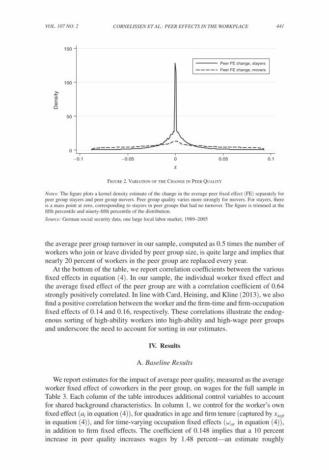
As explained in Section IIA, our baseline specification identifies the causal effect of peers on wages by exploiting two main sources of variation in peer quality: changes to the peer group make-up as workers join and leave the group, and moves to new peer groups by the focal worker. In Figure 2, we plot the kernel density esti-mates of the change in a worker’s average peer quality from one year to the next separately for those who remain in the peer group (stayers) and those who leave (movers). Not surprisingly, the standard deviation of the change in average peer quality is more than three times as high for peer group movers than for peer group stayers (0.20 versus 0.06; see also Table 2). Yet even for workers who remain in their peer group, there is considerable variation in average peer quality from one year to the next, corresponding to roughly 20 percent of the overall variation in average peer quality. As expected, for peer group stayers, the kernel density has a mass point at zero, corresponding to stayers in peer groups that no worker joins or leaves. Nonetheless, peer groups without turnover are rare. In our sample, 90 percent of observations are in peer groups with at least some worker turnover. At 20 percent,

firm-fixed effects, the firm-occupation fixed effects are identified not only through worker mobility across firms, but also through worker mobility between occupations within firms.

Table 2—Structure of Sample

Panel structure(i) Number of workers 2,115,544 (ii) Number of firms 89,581 (iii) Number of peer groups (occupations within firm years) 1,387,216(iv) Average number of time periods per worker 6.07(v) Number of peer groups per firm year 2.30(vi) Average number of employers per worker 1.60(vii) Average number of occupations per worker 1.40(viii) Share of mobility group with identified firm fixed effects 0.995(ix) Share of mobility group with identified firm-time fixed effects 0.994(x) Share of mobility group with identified firm-occupation fixed effects 0.983

Variation in wages, peer quality, and worker turnover(xi) Standard deviation worker fixed effect 0.32(xii) Standard deviation average peer fixed effect 0.24(xiii) Standard deviation change of average peer fixed effect from t − 1 to t 0.09(xiv) Standard deviation change of average peer fixed effect from t − 1 to t − Movers 0.20(xv) Standard deviation change of average peer fixed effect from t − 1 to t − Stayers 0.06(xvi) Share of worker-year observations in peer groups with turnover 0.90(xvii) Average share of workers replaced by turnover 0.20(xviii) Correlation worker fixed effect/average peer fixed effect 0.64(xix) Correlation worker fixed effect/ firm-time effect 0.14(xx) Correlation worker fixed effect/ firm-occupation effect 0.16

Notes: The table shows descriptive statistics describing the panel structure of the dataset, as well as the variation in wages, peer quality and worker turnover which we exploit in subsequent estimations. N = 12,832,842.



the average peer group turnover in our sample, computed as 0.5 times the number of workers who join or leave divided by peer group size, is quite large and implies that nearly 20 percent of workers in the peer group are replaced every year.

At the bottom of the table, we report correlation coefficients between the various fixed effects in equation (4). In our sample, the individual worker fixed effect and the average fixed effect of the peer group are with a correlation coefficient of 0.64 strongly positively correlated. In line with Card, Heining, and Kline (2013), we also find a positive correlation between the worker and the firm-time and firm-occupation fixed effects of 0.14 and 0.16, respectively. These correlations illustrate the endog-enous sorting of high-ability workers into high-ability and high-wage peer groups and underscore the need to account for sorting in our estimates.

IV. Results

A. Baseline Results

We report estimates for the impact of average peer quality, measured as the average worker fixed effect of coworkers in the peer group, on wages for the full sample in Table 3. Each column of the table introduces additional control variables to account for shared background characteristics. In column 1, we control for the worker’s own fixed effect ( a i in equation (4)), for quadratics in age and firm tenure (captured by x iojt in equation (4)), and for time-varying occupation fixed effects ( ω ot in equation (4)), in addition to firm fixed effects. The coefficient of 0.148 implies that a 10 percent increase in peer quality increases wages by 1.48 percent—an estimate roughly

0

0 0.05 0.1−0.05−0.1

50

De

nsi

ty

100

150

x

Peer FE change, stayers

Peer FE change, movers

Figure 2. Variation of the Change in Peer Quality

Notes: The figure plots a kernel density estimate of the change in the average peer fixed effect (FE) separately for peer group stayers and peer group movers. Peer group quality varies more strongly for movers. For stayers, there is a mass point at zero, corresponding to stayers in peer groups that had no turnover. The figure is trimmed at the fifth percentile and ninety-fifth percentile of the distribution.



similar in magnitude to those reported by Lengermann (2002) and Battisti (2013) in a related specification. While this specification accounts for the possibility that work-ers employed in high-wage firms work with better peers, it does not allow for firms which overpay specific occupations relative to the market to attract better workers into these occupations. To deal with this type of worker sorting, we control in column 2 for firm-occupation fixed effects ( θ oj in equation (4)) instead of simple firm fixed effects. This specification produces a much smaller estimate: a 10 percent increase in peer quality now increases the individual wage by only 0.66 percent. It does not yet filter out time-varying shocks at firm level common to all occupations in the firm. Such shocks turn out to be important: When adding time-varying firm fixed effects ( δ jt in equation (4)) in column 3, we find that a 10 percent increase in peer quality raises individual wages by merely 0.1 percent. Translated into standard deviations, this out-come implies that a one standard deviation increase in peer ability increases wages by 0.3 percentage points or 0.6 percent of a standard deviation. This effect is about 10–15 times smaller than the effects previously identified for productivity among supermar-ket cashiers in a single firm (Mas and Moretti 2009) and students carrying out a simple task in an experiment (Falk and Ichino 2006)—which incidentally are very close to the average effect reported by Herbst and Mas (2015) from a larger range of studies mostly covering specific field or lab settings. Therefore, we do not confirm similarly large spillover effects in wages for a representative set of occupations and firms.

B. Effects for Occupational Subgroups

Repetitive Occupations.—Even if peer effects in wages are small on average for a representative set of occupations, they might still be substantial for specific occupations. Hence, in panel A of Table 4, we report the results for the 5 percent

Table 3—Peer Effects in the Full Sample

Observables, occupation-year, and

firm fixed effects(1)

Plus firm-occupation

fixed effects(2)

Plus firm-occupation and firm-year fixed

effects(3)

Average peer fixed effect 0.148 0.066 0.011(0.002) (0.002) (0.001)

Worker fixed effects Yes Yes Yes

Occupation × year effects Yes Yes Yes

Firm effects Yes — —

Occupation × firm effects — Yes Yes

Firm × year effects — — Yes

Notes: The table shows the effect of average peer quality on the individual log wage in the overall sample. Peer quality is measured as the average fixed worker effect of the coworkers in the same three-digit occupation at the same firm in the same point of time. In column 1, we only control for worker fixed effects, firm fixed effects, occupation-by-year fixed effects, and quadratics in age and firm tenure. We then successively add firm-occupation fixed effects (column 2), and firm-by-year fixed effects (column 3). Specification (3) corresponds to the baseline specification described in equation (4) in the text. Coefficients can approximately be interpreted as elasticities, and the coefficient of 0.011 in the baseline specification in column 3 implies that a 10 percent increase in average peer quality increases wages by 0.1 percent. Bootstrapped standard errors with clustering at firm level in parentheses. N = 12,832,842.



of occupations with the most repetitive and predefined tasks, in which we expect particularly high peer pressure. These occupations also more closely resemble those used in earlier studies on peer pressure. The first three columns in the table refer to the baseline specification given by equation (4) and condition on occupation-year, firm-year, and firm-occupation fixed effects, meaning that they correspond to speci-fication (3) in the previous table.

For these repetitive occupations, we find a substantially larger effect of peer qual-ity on wages than in the full sample: a 10 percent increase in peer quality raises wages by 0.64 percent (see column 1) compared to the effect of 0.1 percent in the full sample (see column 3 of Table 3). This outcome implies that a one standard devi-ation increase in peer quality increases the wage by 0.84 percent, about one-half the size of the peer effects in coworker productivity identified by Mas and Moretti (2009) and Falk and Ichino (2006) and in the meta-analysis by Herbst and Mas (2015).

Table 4—Peer Effects in Subsamples of Occupations

Panel A. Peer effects for subsamples of low-skilled occupations

Baseline specification of equation (4)

Within–peer group estimator of

equation (6)

5% most repetitive

occupations

As in case

studies

Low learning content

5% most repetitive

occupations (1) (2) (3) (4)

Average peer fixed effect 0.064 0.067 0.052 0.061(0.0070) (0.0116) (0.0031) (0.006)

Panel B. Peer effects for subsamples of high-skilled occupations

Baseline specification of equation (4)

Within–peer group estimator of

equation (6)

10% most skilled

occupations

10% most innovative

occupations

High learning content

10% most skilled

occupations (1) (2) (3) (4)

Average peer fixed effect 0.013 0.007 0.017 0.016 (0.0039) (0.0044) (0.0028) (0.004)

Notes: The first three columns of the table replicate the baseline peer effects estimates of column 3 in Table 3 for different occupational groups. See online Appendix Table F.3 for a full list of occupations in each of the subsamples used in this table, and Section IIIC in the text for a description of the way in which the different subsamples were constructed. In panel A, column 1, we show the effect for the 5 percent most repetitive occupations. In panel A, col-umn 2, we show the effect for agricultural helpers, cashiers and data entry workers, which have been used in related case-studies on peer effects in the workplace. In panel A, column 3, we report the effect for occupations character-ized by standardized tasks (as the 5 percent most repetitive occupations) and limited learning content (i.e., cashiers, warehouse workers, drivers, removal workers, cleaners, agricultural helpers, and waiters). In panel B, column 1 we present results for the 10 percent most skilled occupations, as measured by the share of workers with a college degree in that occupation. In panel B, column 2 we present results for the 10 percent most innovative occupations, defined by occupation averages of workers’ responses to an index of how frequently they need to experiment with new ideas. In panel B, column 3 we present results for occupations with complex tasks and a high learning content (such as doctors, lawyers, scientists, teachers, and academics). In column 4, we present the within–peer group esti-mate for, as in column 1, the 5 percent most repetitive and 10 percent most skilled occupations, see equation (6) in the text. The within-estimator is based on pre-estimated worker fixed effects from the baseline model in equation (4) in the text. Bootstrapped standard errors with clustering at firm level in parentheses. N = 12,832,842.



Column 2 of panel A shows the peer effect for the three occupations used in earlier studies (agricultural helpers, cashiers, and data entry workers), which is remarkably similar in magnitude to that for the 5 percent most repetitive occupations shown in column 1. Column 3 reports the results for the handpicked group of occupations in which we expect easily observable output and, following initial induction, lim-ited on-the-job learning. The estimated effect for this occupational group is slightly smaller than that for the 5 percent most repetitive occupations sample but still about five times as large as the effect for the full occupational sample.

Column 4 reports estimates using the within–peer group estimator for the 5 per-cent most repetitive occupations (see equation (6)). As we point out above, this estimator is robust to unobserved time-varying peer group wage shocks that are correlated with shocks to true or estimated peer group quality. The estimated peer effects based on the within–peer group specification is very close to the effect derived in the respective baseline specification. This similarity in estimates corroborates that time-varying peer group-specific wage shocks are not important, and provides reas-surance that we are picking up a true peer effect rather than a spurious correlation.

High-Skilled Occupations.—In panel B of Table 4, we restrict the analysis to particularly high-skilled and innovative occupations with a high scope for learning, in which we expect knowledge spillover to be important. Yet regardless of how we define high-skilled occupations (columns 1 to 3), and whether or not we exploit variation in peer ability within peer groups only (column 4), peer effects in these groups are small and resemble those in the full sample. Overall, therefore, we iden-tify sizeable peer effects in wages only in occupations characterized by standard-ized tasks and low learning content, which are exactly the occupations in which we expect peer pressure to matter and which closely resemble the specific occupations investigated in the extant studies on peer pressure.

By looking at the 5 percent most repetitive and the 10 percent most skilled occu-pations we have distinguished between the two extreme ends of the two indexes of repetitiveness and skill from which the definition of these groups was derived. In Figure 3 we show results from a more complete analysis that lets the peer effect coefficient vary by bins of these two indexes. They show a symmetric pattern, with highest peer effects in the most repetitive/least skilled categories, smallest peer effects in the middle categories, and again slightly higher but still small effects in the least repetitive/most skilled categories.14 The U-shape of the estimated peer effects in these indexes provides support for our hypothesis that peer pressure and knowledge spillover are two possible mechanisms for peer effects, where the former operates predominantly in the most repetitive (and least skilled) occupations, while the latter is most pronounced in the least repetitive and most skilled occupations.

C. Timing of Effects

Figure 4 provides a first visual impression of the timing of the wage response to a change in peer quality in the 5 percent most repetitive occupations where peer

14 The skill and repetitiveness indexes are strongly correlated with a correlation coefficient of −0.76.


effects are largest. Panels A and B show the evolutions of peer quality and residual-ized wages (purged of the observables and fixed effects included in equation (4)) of peer group stayers experiencing an exceptionally large rise or fall in peer quality (of at least 0.055), while panel C depicts the corresponding evolutions for peer group movers experiencing an increase in peer quality (of at least 0.10). The figures illus-trate that for both peer group stayers and movers, the increase (or decrease) in peer quality is accompanied by an immediate increase (or decrease) in wages in the same year, with little evidence for dynamic effects.15

We analyze the timing of peer effects more systematically in Table 5, by includ-ing lags and leads of peer quality (computed from the estimated worker fixed effects from the baseline model). In column 1 of Table 5, we first augment our baseline model by adding the quality of a worker’s peers in two future periods (t + 1 and t + 2). The inclusion of future peer quality represents a placebo test, as workers cannot feel peer pressure or learn from colleagues whom they have not yet met. Reassuringly, we find that the effect of future peers is essentially zero in both repet-itive (panel A) and high-skilled occupations (panel B), whereas the effect of current peers remains of the same magnitude as in our baseline specification.

In column 2 of Table 5, we add the average worker fixed effects for the peer group lagged by one and two periods into our baseline regression. The effects of lagged peer quality are informative about the mechanisms for peer effects: If peer effects are generated by peer pressure, then past peers should be irrelevant conditional on current peers in that workers should feel peer pressure only from these latter. If, on the other hand, peer effects result from learning, both past and current peers should matter,

15 It should be noted that any visual illustration of the relationship between two continuously varying variables (peer quality and wages) in an event study graph will necessarily select the underlying sample and reduce the sam-ple size. For instance, workers in the most repetitive occupations who have been with the same firm for at least five periods, and have experienced a rise in peer quality of at least 0.055 in period zero (the “event”), are more likely to be in small peer groups, because the average of peer quality is more variable in small groups and thus large rises are more common. It should therefore not be surprising if the graphical examples slightly deviate from the overall estimates that use the entire sample.

5%most repetitive

5−25%

25−50%

50−75%

75−90%

10%least repetitive

−0.02 0 0.02 0.04 0.06 −0.02 0 0.02 0.04 0.060.08

5%least skilled

5−25%

25−50%

50−75%

75−90%

10% most skilled

Peer effect

Panel A. Peer effect against repetitiveness index Panel B. Peer effect against skill index

95% lower CI/upper CI

Per

cent

ile r

ange

s of

re

petit

iven

ess

inde

x

Per

cent

ile r

ange

s of

sk

ill in

dex

Figure 3. Additional Heterogeneity of the Peer Effect across Bins of the Repetitive and Skilled Index

Notes: The graphs plot the peer effect across bins of the repetitiveness and the skill index. The bottom bar in panel A of the figure corresponds to the 5 percent most repetitive occupations used in previous tables (as in column 1, panel A of Table 4), and the top bar in panel B of the figure corresponds to the 10 percent most skilled occupations used in previous tables (as in column 1, panel B of Table 4).Source: German social security data, one large local labor market, 1989–2005


Panel A. Rise in peer quality: Stayers

Panel B. Fall in peer quality: Stayers

Panel C. Rise in peer quality: Movers

0.68

0.7

0.72

0.74

0.76

0.78

0.72

0.65

0.7

0.75

0.8

0.85

0.74

0.76

0.78

0.8

0.054

0.052

0.05

0.048

0.046

Pee

r qu

ality

Pee

r qu

ality

Pee

r qu

ality

Res

idua

lized

wag

es

0.054

0.08

0.06

0.04

0.02

0.052

0.05

0.048

0.046

Res

idua

lized

wag

esR

esid

ualiz

ed w

ages

−3 −2 −1 0 1

Event time

−3 −2 −1 0 1

Event time−3 −2 −1 0 1

Event time

−3 −2 −1 0 1

Event time−3 −2 −1 0 1

Event time

−3 −2 −1 0 1

Event time

Figure 4. Wage Variation Induced by Changes in Peer Quality (5 Percent Most Repetitive Occupations)

Notes: The figures show, for the 5 percent most repetitive occupations, the evolution of peer quality with an excep-tionally large rise and fall in peer quality (greater than 0.055 from period −1 to period 0) on the left-hand side, and the corresponding evolution of residualized wages for peer group stayers (in panels A and B) in these peer groups on the right-hand side. Average peer quality and residualized wages are shown three periods before and two periods after the large change in peer quality. Panel C shows the evolution of peer quality and residualized wages for individuals who have moved peer group in period 0 and experienced an accompanying rise in peer quality of greater than 0.10, but have stayed in the same peer group in the pre and post periods. Residualized wages have been obtained by a regression of the wage level on fixed effects and observables and are purged of the observables and fixed effects included in baseline equation (4) in the text (except for peer effects, which are not netted out). Sample sizes: 3,432 individuals (panel A), 326 individuals (panel B), 4,989 individuals (panel C).Source: German social security data, one large local labor market, 1989–2005


since the skills learned from a coworker should be valuable even after the worker or coworker has left the peer group. We find that in the repetitive sector, the average quality of lagged peers has almost no effect on current wages, suggesting that knowl-edge spillover is not the primary channel of the peer effects in that sector. Relative to the contemporaneous effect, the lagged effects are slightly more important in skilled occupations (columns 2 and 3 of panel B Table 5), but overall effects continue to be very small. The general pattern of results that only contemporary peer quality matters does not change when including lags and leads jointly in column 3 of Table 5.

D. Geographically and Economically Close Workers Outside of the Immediate Peer Group

In Table 6, we further assess whether the quality of workers outside of the imme-diate peer group affects wages. While providing a test of whether our peer group

Table 5—Timing of Effects

(1) (2) (3)

Panel A. Five percent most repetitive occupationsAverage peer fixed effect 0.066 0.046 0.036

(0.005) (0.005) (0.007)Average peer fixed effect, t + 1 0.006 0.003

(0.005) (0.006)Average peer fixed effect, t + 2 0.001 0.004

(0.005) (0.006)Average peer fixed effect, t − 1 0.0006 0.008

(0.004) (0.005)Average peer fixed effect, t − 2 −0.007 −0.001

(0.004) (0.005)

Observations 392,937 392,937 250,911

Panel B. Ten percent most skilled occupationsAverage peer fixed effect 0.017 0.020 0.016

(0.003) (0.004) (0.005)Average peer fixed effect, t + 1 −0.002 0.007

(0.004) (0.006)Average peer fixed effect, t + 2 −0.006 −0.017

(0.003) (0.007)Average peer fixed effect, t − 1 −0.002 0.004

(0.004) (0.005)Average peer fixed effect, t − 2 0.008 0.012

(0.005) (0.006)

Observations 815,052 815,052 522,338

Notes: The table investigates the dynamic effects of average peer quality on log wages, based on pre-estimated fixed effects from the baseline specification. Panel A shows results for the group of the 5 percent most repetitive occupations, as in column 1, panel A of Table 4. Panel B reports results for the group of the 10 percent most skilled occupations, as in column 1, panel B, of Table 4. In column 1 we add the peer quality of the focal worker’s future peers from the periods t + 1 and t + 2 to our baseline specification as a placebo test. In column 2 we add the average fixed effects of the lagged peer group to equation (4). In column 3 we present a more complete specification including both leads and lags. Bootstrapped standard errors with clustering at firm level in parentheses.



definition is appropriate, the results also shed light on the potential channel of peer effects. In the case of peer pressure, the relevant peers are contemporaneous cowork-ers in the immediate peer group within the firm who frequently interact and carry out comparable tasks, as peer pressure can only build up if workers work alongside each other and can observe and compare each other’s output. If, in contrast, peer

Table 6—Other Peer Groups Inside and Outside the Firm

5% most repetitive occupations

10% most skilled occupations

(1) (2)

Panel A. Economically close and far peer groups within the same firm(i) Other occupation in the same firm with above-median −0.0006 −0.0005

closeness (“close”) (0.0009) (0.0011)(ii) Other occupation in the same firm with below-median −0.0009 0.0007

closeness (“far”) (0.0005) (0.0012)(iii) “Closest” other occupation in the same firm −0.0162 0.0097

(0.0050) (0.0037)(iv) “Farthest” other occupation in the same firm −0.020 −0.018

(0.004) (0.003)

Panel B. Economically close peer groups in other firms(i) Average worker fixed effect of own peer group 0.0841 0.0134

(0.0034) (0.0031)(ii) Average worker fixed effect in economically close peer −0.0012 −0.0004

groups in other firms (0.0015) (0.0010)(iii) Average worker fixed effect of joiners’ past peers −0.0008 0.0002

(0.0007) (0.0006)

Panel C. Geographically close peers outside the firm(i) Average worker fixed effect of own peer group 0.0758 0.0202

(0.0074) (0.0038)(iii) Average peer fixed effect in municipality 0.0029 −0.0035

(0.0043) (0.0033)

Notes: The table reports effects on log wages of the peer quality in peer groups that are economically or geographi-cally close (or far) to the focal worker’s own peer group. Column 1 shows the results for the group of the 5 percent most repetitive occupations, as in column 1, panel A of Table 4. Column 2 reports results for the group of the 10 per-cent most skilled occupations, as in column 1, panel B, of Table 4. In rows (i) and (ii) of panel A, we report results when the peer group consists of workers from a randomly chosen three-digit occupation (other than the worker’s own occupation) in the same firm; distinguishing whether the randomly assigned peer group is from an economi-cally “close” or an economically “far” occupation, where economic closeness is measured by worker flows between occupations in the overall sample. A pair of occupations is defined as “close” if the proportion of workers switch-ing between these occupations is above median, and “far” if it is below median. This specification drops firm-year observations with only one occupation. In rows (iii) and (iv) of panel A, we show the effect of peer quality in the economically closest and farthest three-digit occupation (other than the worker’s own occupation) in the same firm, where closeness is again measured by worker flows between occupations in the overall sample. This specification is based on firm-year observations with at least three occupations per firm. In panel B, we report results when adding peer quality of workers in peer groups in other firms that are economically close to the focal worker’s peer group to our baseline specification, where we again measure economic closeness by worker flows in the overall sample. In row (ii), we report the coefficient on the average worker fixed effect of workers who in year t are in peer groups ( firm-occupation combinations) in other firms that at any point during the observation period have exchanged work-ers with the focal worker’s peer group. In row (iii), we report the coefficient on the peer quality of the past peers of recent joiners to the focal worker’s peer group. For this we first identify the peer groups from which new joiners to the focal peer group came (i.e., the peer groups in which the joiners were in t − 1) and compute the average worker fixed effect of the workers who were in these peer groups in t − 1 but who did not join the focal peer group t. In panel C, we augment the baseline model by adding the average peer quality of workers living in the same munic-ipality who are employed in the same occupation (but not necessarily in the same firm) as the focal worker. This equation is run on a sample for the period 1999–2010 because the indicator of the municipality of residence is only available from 1999. Bootstrapped standard errors with clustering at firm level in parentheses.



effects result from knowledge spillover, a much wider group of peers is potentially relevant, since knowledge spillover is not restricted to occur within the firm only. In fact, knowledge spillover is often assumed to operate through interactions of workers who do not necessarily work in the same firm but are geographically or economically close (see, e.g., Lucas 1988; Moretti 2004).

In panel A of Table 6, we estimate the effects of the quality of workers in other occupations within the same firm on wages. In rows (i) and (ii) of panel A, we ran-domly choose a three-digit occupation (other than the worker’s own occupation) in the same firm, and distinguish whether the randomly assigned occupation is eco-nomically close or far, as measured by observed worker flows between occupations in the overall sample.16 The results show that in both the repetitive and skilled sec-tor, the quality of coworkers in other occupations within the same firm has virtually no impact on wages, no matter whether the occupation is close or far. We corrobo-rate these findings in rows (iii) and (iv) of panel A, where we display the impact on wages of the quality of workers in the economically closest and farthest occupation (relative to the focal worker’s own occupation) in the same firm, again measuring economic closeness by observed worker flows between occupations in the overall sample. Overall, these findings provide strong evidence for the validity of defining the peer group as workers from the same three-digit occupation in the same firm, and speak against knowledge spillover or peer pressure across occupations within the same firm.

In panel B of Table 6, we augment our baseline model by adding the quality of workers in other firms that are economically close (in terms of worker flows) to the focal worker’s peer group. First, we include the average peer fixed effect of workers who in year t are in peer groups ( firm-occupation combinations) in other firms that at any point during the observation period have exchanged workers with the focal worker’s peer group. Second, we identify the peer groups from which new joiners to the focal peer group came (i.e., the peer groups in which the joiners were in t − 1), and we add the average worker fixed effect of the workers who were in these peer groups in t − 1 but who did not join the focal peer group (i.e., the joiners’ past peers). Effects from these economically close workers in other firms are virtually zero, providing little evidence for knowledge spillover across peer groups in differ-ent firms linked by worker mobility.

In panel C of Table 6 we augment our baseline model by adding the average fixed effect of all workers residing in the same municipality and working in the same occupation (but not necessarily in the same firm) as the focal worker. We find that peer quality in the municipality has no effect on wages, whereas the effect of peer quality in the firm remains unchanged.

In sum, the results in Table 6 provide little evidence of knowledge spillover or peer pressure from workers outside the immediate peer group. Rather, they suggest that peer effects in the repetitive sector are confined to the same three-digit occupa-tion and firm, as one would expect if peer pressure is the main driving force behind peer effects.

16 We define a pair of occupations as “close” if the proportion of workers switching between these occupations is above median, and “far” if it is below median.


E. Robustness Checks

As Table 7 shows, estimated peer effects remain robust to a number of alter-native specifications for both the repetitive (column 1) and the high-skilled sector (column 2). As a point of reference, row (i) replicates the results from the baseline specification of column 1, Table 4.

As illustrated in Figure 2, our baseline specification exploits two sources of vari-ation in peer quality: changes to the peer group makeup as coworkers join and leave the group, and moves to new peer groups by the focal worker. Unlike the latter, the former controls for the presence of time-constant match-specific effects m ioj that are correlated with peer ability (as first differencing eliminates these for peer group stayers, but not for peer group movers). Rows (ii) and (iii) show that both sources of variation lead to very similar peer effects, indicating that our baseline peer estimates are not biased because of match-specific shocks.17

In row (iv), we report results when the censored wage observations are not imputed. In row (v), we relax the assumption that observable characteristics have the same effects in repetitive occupations and high-skilled occupations. In row (vi), we extend our estimation sample to include not only the metropolitan area of Munich, but also additional surrounding rural areas. In row (vii), we add to the regression the average observed characteristics (firm tenure, age, and schooling) of peers. In rows (viii) and (ix), we display peer effect estimates separately for small (≤ 10) and large (> 100) peer groups.18 Remarkably, for both repetitive and high-skilled occupations, all these different specifications yield similar estimates as the baseline estimates reported in Table 4.

The evidence presented in panel A of Table 6 suggests that workers rarely interact with coworkers outside the same three-digit occupation in the firm, supporting the definition of the peer group as workers from the same three-digit occupation, rather than the same two- or one-digit occupation, in the same firm. In row (x) of Table 7, we display peer effect estimates for a narrower peer group definition where we split peer groups at the three-digit occupational level further up into two age groups (above and below median age). Interestingly, the peer effect drops by more than 50 percent, which is in line with the hypothesis that the exclusion of relevant peers from the peer group leads to an attenuation bias. Overall, this drop, in conjunction with the findings in panel A of Table 6, suggests that our baseline peer group defini-tion at the three-digit occupational level is the most plausible.19

17 This is in line with Card, Heining, and Kline (2013) and Card, Cardoso, and Kline (2016), who show that once firm fixed effects are accounted for, match-specific effects are not an important determinant of worker mobility.

18 In online Appendix Table F.4, we display estimates for finer peer group size and firm size categories. The estimates are very similar across the different categories of peer group and firm sizes for both most repetitive and high-skilled occupations.

19 As a further robustness check, we have instrumented, for the 5 percent most repetitive occupations, the change in peer quality by the average quality of leavers from the peer group who in t − 1 were close to retirement age; the rationale being that leaving into retirement may be more exogenous than other reasons for the turnover of peers. This gives us a strong first stage ( F-value 151.1) with expected negative sign. The IV peer effect coefficient is 0.041, not too far off our baseline estimate of 0.064, although imprecisely estimated and not statistically significant; see Table F.5 in the online Appendix.


F. Heterogeneous Peer Effects

We now provide additional evidence that peer effects in the 5 percent most repet-itive occupations—where we have found the strongest effects—are driven primarily by peer pressure, by investigating heterogeneity in peer effects in that sector.

Age and Job Tenure.—In the low-skilled, repetitive occupations we consider, we expect that almost all the on-the-job learning takes place when workers are young or have only just joined the peer group. In panel A of Table 8, we there-fore allow the peer effect in the 5 percent most repetitive occupations to differ for older (age >35 years) and younger workers (age ≤35 years) and for workers who

Table 7—Robustness Checks

5% most repetitive occupations

10% most skilled occupations

(1) (2)

(i) Baseline 0.064 0.013(0.0070) (0.0039)

(ii) Separate effect for stayers 0.061 0.014(0.006) (0.003)

(iii) Separate effect for movers 0.073 0.006(0.006) (0.004)

(iv) Wage not imputed 0.086 0.017(0.007) (0.007)

(v) Varying coefficients on observables 0.082 0.007(0.008) (0.004)

(vi) Expansion of sample to larger region 0.082 0.014 with additional rural areas (0.008) (0.002)

(vii) Include peer observables 0.071 0.010(0.006) (0.005)

(viii) Peer groups size ≤10 0.068 0.014(0.002) (0.001)

(ix) Peer groups size >100 0.081 0.014(0.004) (0.003)

(x) Peer group defined by age groups within 0.032 0.006 three-digit occupations (0.007) (0.004)

Notes: The table reports a number of robustness checks for the effect of average peer quality on log wages. The first column refers to the group of the 5 percent most repetitive occupations and the second column refers to the group of the 10 percent most skilled occupations. For compar-ison, we replicate the results from the respective baseline specifications of column 1, Table 4 in row (i). In rows (ii) and (iii), we show separate peer effects for stayers and movers. Workers are defined as stayers in periods when they are in the same firm and occupation in period t as in period t − 1, and as movers when they switch the firm or occupation between periods t − 1 and t. In row (iv), we do not impute censored wage observations. In row (v), we allow the coef-ficients on the observable characteristics (quadratics in age and firm tenure) to vary between the 5 percent most repetitive (or 10 percent most skilled) occupations and the remaining occu-pations. In row (vi) we extend our estimation sample to include not only the metropolitan area of Munich, but also additional surrounding rural areas. In row (vii), we augment the baseline model by adding peer averages of observed characteristics (firm tenure, age, and schooling). In rows (viii) and (ix), we report the peer effect coefficient for small and large peer groups respectively. In row (x), we report results for an alternative narrower peer group definition at the three-digit-occupation-age-firm level. Bootstrapped standard errors with clustering at firm level in parentheses. N = 12,832,842.



have been with the peer group for more or less than two years. Although we do find that peer effects are larger for younger workers, which is in line with knowl-edge spillover, we also find positive peer effects for older workers. Moreover, peer effects vary little with tenure in the peer group. Both these findings are difficult to reconcile with peer effects arising from knowledge spillover alone. It should also be noted that although the smaller peer effect for older workers is consistent with knowledge spillover, it is also in line with younger workers responding more strongly to peer pressure or suffering more from the “pain” of peer pressure than older or more experienced workers.

Symmetry of Effects.—In panel B of Table 8 we investigate whether improve-ments in the average peer group quality have similar effects as deteriorations. To this

Table 8—Heterogeneous Peer Effects (5% Most Repetitive Occupations)

Panel A. Heterogeneous effects by age and peer group tenureAge ≤ 35 years Age > 35 years

Average peer fixed effect 0.081 0.053(0.005) (0.005)

Peer group tenure < 2 Peer group tenure ≥ 2Average peer fixed effect 0.058 0.066

(0.007) (0.006)

Panel B. Symmetry of peer effects (first differences, peer group stayers, pre-estimated effects)Negative change Positive change

Change in average peer fixed effect 0.055 0.048(0.010) (0.008)

Panel C. Heterogeneous effects by relative position within the peer groupFocal worker below median

Focal workerabove median

Average peer fixed effect 0.066 0.032(0.006) (0.006)

Panel D. Distinguishing between top versus bottom peers ( pre-estimated)Top versus bottom peers

Average fixed effect of middle 80% peers 0.072(0.0045)

Average fixed effect of top 10% of peers 0.004(0.0018)

Average fixed effect of bottom 10% of peers 0.007(0.0017)

Notes: The table investigates possible heterogeneous effects of peer quality in the 5 percent most repetitive sector. In panel A we allow the effect of average peer quality on log wages to differ between workers below and above age 35, and between workers who have been in the peer group more and less than two years. In panel B we inves-tigate whether improvements and deteriorations in average peer quality have similarly sized effects. To do this, we adopt an approach similar to Mas and Moretti (2009) and regress, for peer group stayers, the change in log wages on the change in peer group quality (using the pre-estimated worker fixed effects from our baseline specification), and allow this effect to vary according to whether peer group quality improved or deteriorated. In panel C we let the peer effect vary by whether the focal worker is above or below the peer-group mean of ability (as measured by the pre-estimated worker fixed effects from the baseline model). In panel D, we split the worker’s peers up into the mid-dle 80 percent, top 10 percent, and bottom 10 percent according to their ability ranking. This specification is again based on pre-estimated worker fixed effects, and is run on the sample for the middle 80 percent of workers only.



end, using the peer group stayers, we regress the change in log wages on the change in peer group quality (using the pre-estimated worker fixed effects from our baseline specification) and allow this effect to vary according to whether peer group quality improves or deteriorates (see Mas and Moretti 2009, for a similar specification). Our results show relatively symmetric effects for both improvements and deterio-rations. This once again points against knowledge spillover as the primary driver behind peer effects in the repetitive sector, as it is unlikely that workers immediately “unlearn” skills when peers get worse.

Low- versus High-Ability Workers.—In panel C of Table 8, we explore whether the peer effects in wages differ for low- versus high-ability workers in the peer group (i.e., workers with a worker fixed effect, pre-estimated from our baseline specification, below and above the median in the firm-occupation). Like Mas and Moretti (2009), we find that peer effects are almost twice as large for low- as for high-ability workers. One possible explanation is that low-ability workers increase their effort more than high-ability workers in response to an increase in peer quality (i.e., the peer effect in productivity is higher for low- than for high-ability workers). If this latter does indeed explain peer effect differences between low- and high-ability workers, then, as Mas and Moretti (2009) emphasize, firms may want to increase peer group diversity—and maximize productivity—by grouping low-ability with high-ability workers.

Our model, however, also suggests an alternative interpretation; namely, that low-ability workers suffer more from the pain of peer pressure than high-ability workers, leading to higher peer effects in wages for low- than high-ability workers, even when peer effects in productivity are the same.20 If such “pain” is the reason for the larger peer effects among the low-ability workers, then firms may prefer homogeneous peer groups over diverse peer groups because they will save wage costs without lowering productivity.

Bottom versus Top Peers.—Whereas all our previous specifications estimate the effect of average peer quality on wages, in panel D of Table 8, we estimate the effect of the quality of the top and bottom workers in the peer group on wages. To do so, we split the peer group into three groups: the top 10 percent, the middle 80 percent, and the bottom 10 percent of peers based on the estimated worker fixed effects from our baseline regression.21 We then regress individual wages on the average worker fixed effect for the three groups, controlling for the same covariates and fixed effects as in our baseline specification and restricting the sample to workers in the middle group. We find that the effect of the average peer quality in the middle group on wages is similar to our baseline effect, while the average productivities of peers in

20 In our model, low- and high-ability workers increase their effort by the same amount in response to an increase in peer ability (see online Appendix equation (A.2)), meaning that the peer effect in productivity is the same for both groups. Note, however, that the rate at which higher peer ability translates into “pain” from peer pressure,

∂ P ( e i ,

_ y ~i ) _______ ∂ _ y ~i = λ P (m − e i ⁎ ) varies inversely with a worker’s own optimal effort e i ⁎ , which in turn varies positively

with individual ability (see online Appendix equation (A.4)), implying that the pain from peer pressure for a given

increase in peer ability is higher for low-ability than for high-ability workers. 21 Although these shares are quite exact in large peer groups, in small peer groups, the top and bottom do not

exactly equal 10 percent. For example, in a peer group with four workers, one worker falls at the top, one at the bottom, and two in the middle.


the bottom or top groups have no significant effect on wages. Hence, our baseline peer effects are neither driven entirely by very bad workers nor driven entirely by very good workers. This observation rules out a simple chain production model in which team productivity is determined by the productivity of the “weakest link in the chain”; that is, the least productive worker. It also suggests that the peer effects in the 5 percent most repetitive occupations are not driven solely by the most pro-ductive workers in the peer group, even though these latter may increase overall peer group productivity by motivating and guiding their coworkers.22

V. Conclusions

Although peer effects in the classroom have been extensively studied in the liter-ature (see Sacerdote 2011, for an overview), empirical evidence on peer effects in coworker productivity is as yet restricted to a handful of studies based on either lab-oratory experiments or real-world data from a single firm or occupation. Our study sheds light on the external validity of these studies by carrying out the first investi-gation to date into peer effects in a general workplace setting. Unlike the previous research, our study focuses on peer effects in wages rather than in productivity.

On average we find only small, albeit precisely estimated, peer effects in wages, suggesting that the larger peer effects found in existing studies may not carry over to the labor market in general. Yet our results also reveal larger peer effects in low-skilled occupations where coworkers can easily observe each other’s output, which are exactly the occupations most often analyzed in the previous studies on peer pres-sure. In these types of occupations, therefore, the findings of previous studies extend beyond the specific firms or tasks which they explore. Our results also indicate that in this segment of the labor market, productivity spillovers translate into wage spill-overs—a dynamic as yet unexplored in the literature—and suggest that indeed peer pressure, and not knowledge spillover, is the main source of the peer effect.

Overall, we conclude that peer effects in the workplace, despite being important in some specific settings, do not importantly affect the wage setting of firms, nor do they contribute significantly to overall inequality in the labor market.

REFERENCES

Abowd, John M., Francis Kramarz, and David N. Margolis. 1999. “High Wage Workers and High Wage Firms.” Econometrica 67 (2): 251–333.

Ammermueller, Andreas, and Jorn-Steffen Pischke. 2009. “Peer Effects in European Primary Schools: Evidence from the Progress in International Reading Literacy Study.” Journal of Labor Econom-ics 27 (3): 315–48.

Arcidiacono, Peter, Gigi Foster, Natalie Goodpaster, and Josh Kinsler. 2012. “Estimating Spillovers Using Panel Data, with an Application to the Classroom.” Quantitative Economics 3 (3): 421–70.

Azoulay, Pierre, Joshua S. Graff Zivin, and Jialan Wang. 2010. “Superstar Extinction.” Quarterly Journal of Economics 125 (2): 549–89.

22 In an interesting study in a technology-based services company, Lazear, Shaw, and Stanton (2015) find that the quality of bosses has significant effects on the productivity of their subordinates. While it might be tempting to interpret the quality of the top 10 percent of peers in our study as a proxy for boss quality, we prefer not to interpret our findings as informative on boss effects: first, we cannot ascertain whether more able peers are indeed more likely to become team leaders or supervisors, and second, bosses need not necessarily belong to the same occupa-tion as their subordinates and thus need not be in the same peer group as defined by our data.

http://pubs.aeaweb.org/action/showLinks?crossref=10.1111%2F1468-0262.00020

http://pubs.aeaweb.org/action/showLinks?crossref=10.1086%2F603650

http://pubs.aeaweb.org/action/showLinks?crossref=10.3982%2FQE145

http://pubs.aeaweb.org/action/showLinks?crossref=10.1162%2Fqjec.2010.125.2.549


Babcock, Philip, Kelly Bedard, Gary Charness, John Hartman, and Heather Royer. 2015. “Letting Down the Team? Social Effects of Team Incentives.” Journal of the European Economic Associa-tion 13 (5): 841–70.

Bandiera, Oriana, Iwan Barankay, and Imran Rasul. 2010. “Social Incentives in the Workplace.” Review of Economic Studies 77 (2): 417–58.

Barron, John M., and Kathy Paulson Gjerde. 1997. “Peer Pressure in an Agency Relationship.” Jour-nal of Labor Economics 15 (2): 234–54.

Battisti, Michele. 2013. “High Wage Workers and High Wage Peers.” University of Munich Ifo Work-ing Paper 168.

Betts, Julian R., and Andrew Zau. 2004. “Peer Groups and Academic Achievement: Panel Evi-dence from Administrative Data.” http://legacy.iza.org/iza/en/webcontent/events/transatlantic/papers_2004/betts.pdf (accessed December 2, 2016).

Bloom, Nicholas, James Liang, John Roberts, and Zhichun Jenny Ying. 2015. “Does Working from Home Work? Evidence from a Chinese Experiment.” Quarterly Journal of Economics 130 (1): 165–218.

Card, David, Ane Rute Cardoso, and Patrick Kline. 2016. “Bargaining, Sorting, and the Gender Wage Gap: Quantifying the Impact of Firms on the Relative Pay of Women.” Quarterly Journal of Eco-nomics 131 (2): 633–86.

Card, David, Jorg Heining, and Patrick Kline. 2013. “Workplace Heterogeneity and the Rise of West German Wage Inequality.” Quarterly Journal of Economics 128 (3): 967–1015.

Chan, Tat Y., Jia Li, and Lamar Pierce. 2014. “Compensation and Peer Effects in Competing Sales Teams.” Management Science 60 (8): 1965–84.

Cornelissen, Thomas. 2016. “Do Social Interactions in the Workplace Lead to Productivity Spillover among Co-Workers?” IZA World of Labor 314 (November).

Cornelissen, Thomas, Christian Dustmann, and Uta Schönberg. 2017. “Peer Effects in the Workplace: Dataset.” American Economic Review. https://doi.org/10.1257/aer.20141300.

De Grip, Andries, and Jan Sauremann. 2012. “The Effects of Training on Own and Co-worker Produc-tivity: Evidence from a Field Experiment.” Economic Journal 122 (560): 376–99.

Dustmann, Christian, Johannes Ludsteck, and Uta Schonberg. 2009. “Revisiting the German Wage Structure.” Quarterly Journal of Economics 124 (2): 843–81.

Falk, Armin, and Andrea Ichino. 2006. “Clean Evidence on Peer Effects.” Journal of Labor Econom-ics 24 (1): 39–57.

Gathmann, Christina, and Uta Schonberg. 2010. “How General Is Human Capital? A Task-Based Approach.” Journal of Labor Economics 28 (1): 1–49.

Gould, Eric D., Victor Lavy, and M. Daniele Paserman. 2009. “Does Immigration Affect the Long-Term Educational Outcomes of Natives? Quasi-Experimental Evidence.” Economic Journal 119 (540): 1243–69.

Gould, Eric D., and Eyal Winter. 2009. “Interactions between Workers and the Technology of Production: Evidence from Professional Baseball.” Review of Economics and Statistics 91 (1): 188–200.

Guryan, Jonathan, Kory Kroft, and Matthew J. Notowidigdo. 2009. “Peer Effects in the Workplace: Evidence from Random Groupings in Professional Golf Tournaments.” American Economic Jour-nal: Applied Economics 1 (4): 34–68.

Hanushek, Eric A., John F. Kain, Jacob M. Markman, and Steven G. Rivkin. 2003. “Does Peer Ability Affect Student Achievement?” Journal of Applied Econometrics 18 (5): 527–44.

Herbst, Daniel, and Alexandre Mas. 2015. “Peer Effects on Worker Output in the Laboratory General-ize to the Field.” Science 250 (6260): 545–49.

Hoxby, Caroline. 2000. “Peer Effects in the Classroom: Learning from Gender and Race Variation.” National Bureau of Economic Research Working Paper 7867.

Ichino, Andrea, and Giovanni Maggi. 2000. “Work Environment and Individual Background: Explain-ing Regional Shirking Differentials in a Large Italian Firm.” Quarterly Journal of Economics 115 (3): 1057–90.

Jackson, C. Kirabo, and Elias Bruegmann. 2009. “Teaching Students and Teaching Each Other: The Importance of Peer Learning for Teachers.” American Economic Journal: Applied Economics 1 (4): 85–108.

Kandel, Eugene, and Edward P. Lazear. 1992. “Peer Pressure and Partnerships.” Journal of Political Economy 100 (4): 801–17.

Kaur, Supreet, Michael Kremer, and Sendhil Mullainathan. 2010. “Self-Control and the Development of Work Arrangements.” American Economic Review 100 (2): 624–28.

http://legacy.iza.org/iza/en/webcontent/events/transatlantic/papers_2004/betts.pdf

http://legacy.iza.org/iza/en/webcontent/events/transatlantic/papers_2004/betts.pdf

http://pubs.aeaweb.org/action/showLinks?crossref=10.1093%2Fqje%2Fqju032

http://pubs.aeaweb.org/action/showLinks?system=10.1257%2Faer.100.2.624



http://pubs.aeaweb.org/action/showLinks?system=10.1257%2Fapp.1.4.34


http://pubs.aeaweb.org/action/showLinks?crossref=10.1093%2Fqje%2Fqjv038


http://pubs.aeaweb.org/action/showLinks?crossref=10.1002%2Fjae.741


http://pubs.aeaweb.org/action/showLinks?crossref=10.1093%2Fqje%2Fqjt006

http://pubs.aeaweb.org/action/showLinks?crossref=10.1111%2Fj.1468-0297.2012.02500.x

http://pubs.aeaweb.org/action/showLinks?crossref=10.1111%2Fjeea.12131


http://pubs.aeaweb.org/action/showLinks?crossref=10.1126%2Fscience.aac9555


http://pubs.aeaweb.org/action/showLinks?crossref=10.1287%2Fmnsc.2013.1840

http://pubs.aeaweb.org/action/showLinks?crossref=10.1162%2Fqjec.2009.124.2.843

http://pubs.aeaweb.org/action/showLinks?crossref=10.1111%2Fj.1467-937X.2009.00574.x

http://pubs.aeaweb.org/action/showLinks?crossref=10.1162%2Frest.91.1.188


Lavy, Victor, M. Daniele Paserman, and Analia Schlosser. 2012. “Inside the Black Box of Ability Peer Effects: Evidence from Variation in the Proportion of Low Achievers in the Classroom.” Economic Journal 122 (559): 208–37.

Lavy, Victor, and Analia Schlosser. 2011. “Mechanisms and Impacts of Gender Peer Effects at School: Corrigendum.” American Economic Journal: Applied Economics 3 (3): 1–33.

Lazear, Edward P., Kathryn L. Shaw, and Christopher T. Stanton. 2015. “The Value of Bosses.” Jour-nal of Labor Economics 33 (4): 823–61.

Lengermann, Paul. 2002. “Is It Who You Are, Where You Work, or with Whom You Work? Reassess-ing the Relationship between Skill Segregation and Wage Inequality.” Longitudinal Employer––Household Dynamics Technical Paper TP-2002-10.

Lindquist, Matthew, Jan Sauermann, and Yves Zenou. 2015. “Network Effects on Worker Productiv-ity.” CEPR Discussion Paper 10928.

Lucas, Robert E., Jr. 1988. “On the Mechanics of Economic Development.” Journal of Monetary Eco-nomics 22 (1): 3–42.

Manski, Charles F. 1993. “Identification of Endogenous Social Effects: The Reflection Problem.” Review of Economic Studies 60 (3): 531–42.

Marshall, Alfred. 1890. Principles of Economics. New York: Macmillan.Mas, Alexandre, and Enrico Moretti. 2009. “Peers at Work.” American Economic Review 99 (1):

112–45.McEwan, Patrick J. 2003. “Peer Effects on Student Achievement: Evidence from Chile.” Economics

of Education Review 22 (2): 131–41.Moretti, Enrico. 2004. “Workers’ Education, Spillovers, and Productivity: Evidence from Plant-Level

Production Functions.” American Economic Review 94 (3): 656–90.Sacerdote, Bruce. 2011. “Peer Effects in Education: How Might They Work, How Big Are They, and

How Much Do We Know Thus Far?” In Handbook of Economics of Education, Vol. 3, edited by Erik Hanushek, Stephen Machin, and Ludger Woessmann, 249–77. Amsterdam: Elsevier.

Serafinelli, Michel. 2013. “Good Firms, Worker Flows and Productivity.” https://www.economics.utoronto.ca/public/workingPapers/tecipa-538.pdf (accessed December 2, 2016).

Vigdor, Jacob L., and Thomas Nechyba. 2007. “Peer Effects in North Carolina Public Schools.” In Schools and the Equal Opportunity Problem, edited by Ludger Woessman and Paul E. Peterson, 73–101. Cambridge, MA: MIT Press.

Waldinger, Fabian. 2010. “Quality Matters: The Expulsion of Professors and the Consequences for PhD Student Outcomes in Nazi Germany.” Journal of Political Economy 118 (4): 787–831.

Waldinger, Fabian. 2012. “Peer Effects in Science: Evidence from the Dismissal of Scientists in Nazi Germany.” Review of Economic Studies 79 (2): 838–61.

https://www.economics.utoronto.ca/public/workingPapers/tecipa-538.pdf

http://pubs.aeaweb.org/action/showLinks?system=10.1257%2F0002828041464623


http://pubs.aeaweb.org/action/showLinks?crossref=10.1093%2Frestud%2Frdr029


http://pubs.aeaweb.org/action/showLinks?system=10.1257%2Faer.99.1.112


http://pubs.aeaweb.org/action/showLinks?crossref=10.1016%2F0304-3932%2888%2990168-7

http://pubs.aeaweb.org/action/showLinks?crossref=10.1016%2FS0272-7757%2802%2900005-5



Documents

Peer Effects in the Workplace