Peer Migration in China

Yuyu ChenPeking University

Ginger JinUniversity of Maryland & NBER

Yang YuePeking University

In collaboration with a local government of China

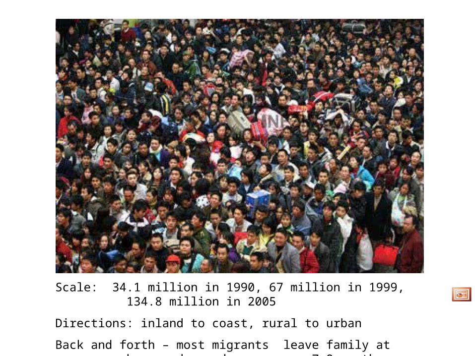
Scale: 34.1 million in 1990, 67 million in 1999, 134.8 million in 2005

Directions: inland to coast, rural to urban

Back and forth – most migrants leave family at home and spend on average 7-8 months a year in the city,

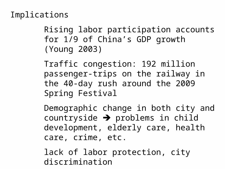
Implications

Rising labor participation accounts for 1/9 of China’s GDP growth (Young 2003)

Traffic congestion: 192 million passenger-trips on the railway in the 40-day rush around the 2009 Spring Festival

Demographic change in both city and countryside problems in child development, elderly care, health care, crime, etc.

lack of labor protection, city discrimination

unemployment waves due to economic recession

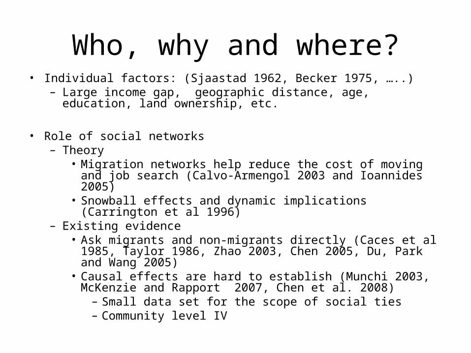
Who, why and where?• Individual factors: (Sjaastad 1962, Becker 1975, …..)

– Large income gap, geographic distance, age, education, land ownership, etc.

• Role of social networks– Theory

• Migration networks help reduce the cost of moving and job search (Calvo-Armengol 2003 and Ioannides 2005)

• Snowball effects and dynamic implications (Carrington et al 1996)

– Existing evidence• Ask migrants and non-migrants directly (Caces et al 1985,

Taylor 1986, Zhao 2003, Chen 2005, Du, Park and Wang 2005)

• Causal effects are hard to establish (Munchi 2003, McKenzie and Rapport 2007, Chen et al. 2008)

– Small data set for the scope of social ties– Community level IV

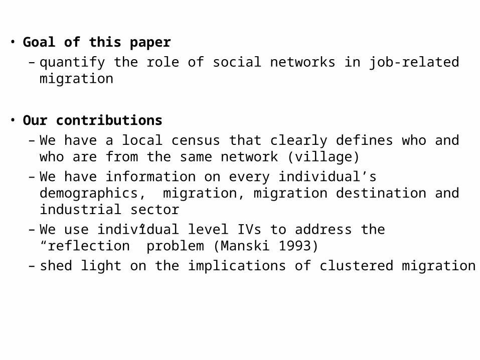
• Goal of this paper

– quantify the role of social networks in job-related migration

• Our contributions

– We have a local census that clearly defines who and who are from the same network (village)

– We have information on every individual’s demographics, migration, migration destination and industrial sector

– We use individual level IVs to address the “reflection” problem (Manski 1993)

– shed light on the implications of clustered migration

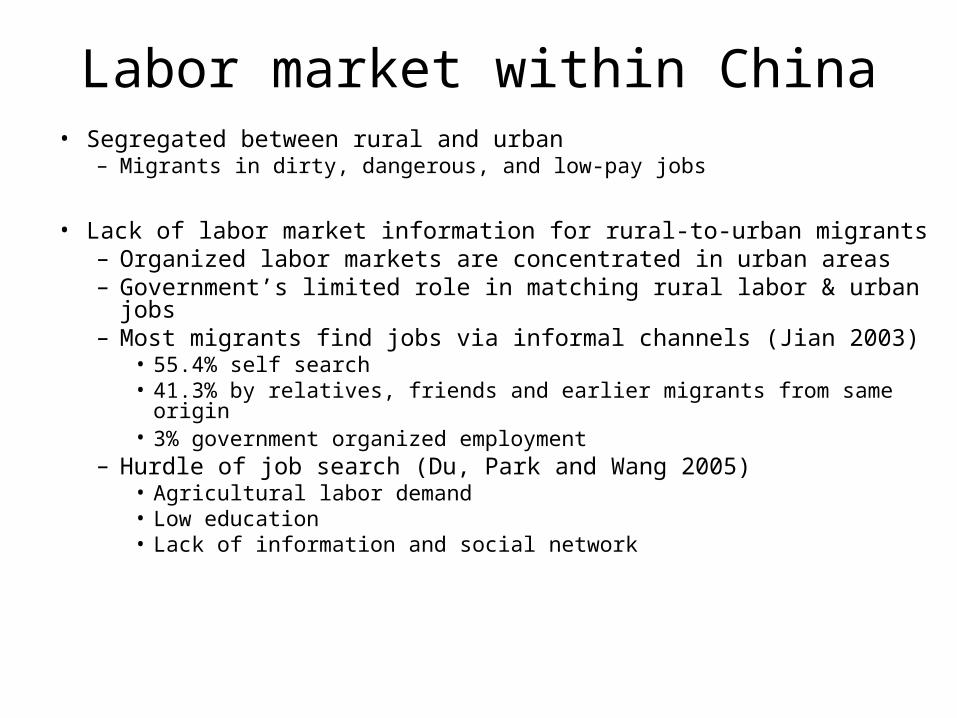
Labor market within China• Segregated between rural and urban

– Migrants in dirty, dangerous, and low-pay jobs

• Lack of labor market information for rural-to-urban migrants– Organized labor markets are concentrated in urban areas– Government’s limited role in matching rural labor & urban jobs– Most migrants find jobs via informal channels (Jian 2003)

• 55.4% self search• 41.3% by relatives, friends and earlier migrants from same origin• 3% government organized employment

– Hurdle of job search (Du, Park and Wang 2005)• Agricultural labor demand• Low education• Lack of information and social network

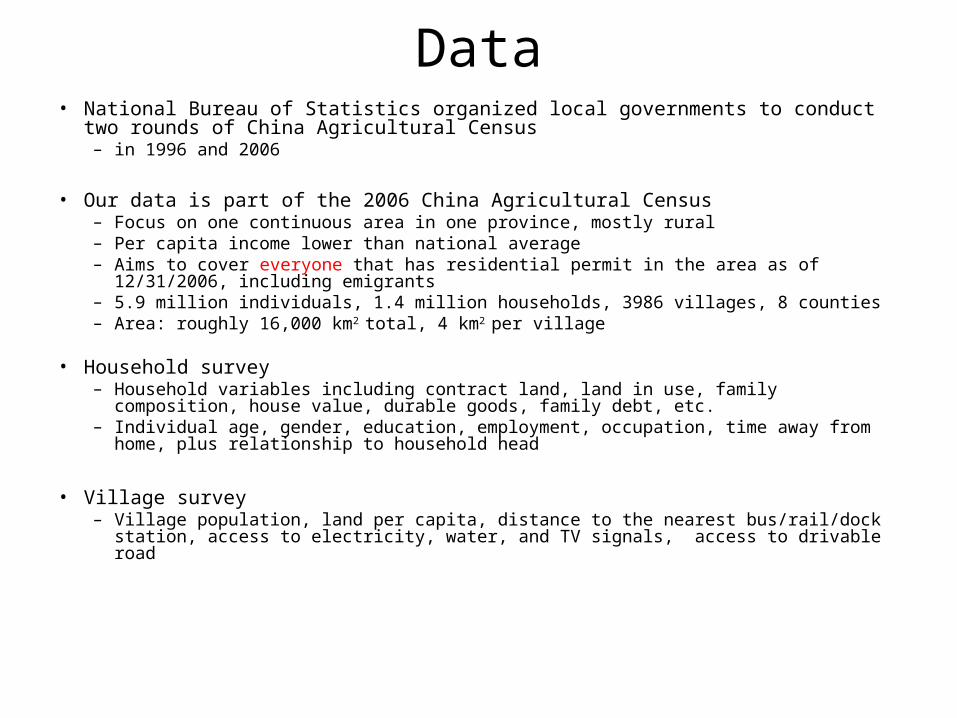
Data• National Bureau of Statistics organized local governments to conduct two rounds of

China Agricultural Census– in 1996 and 2006

• Our data is part of the 2006 China Agricultural Census– Focus on one continuous area in one province, mostly rural– Per capita income lower than national average– Aims to cover everyone that has residential permit in the area as of 12/31/2006, including

emigrants– 5.9 million individuals, 1.4 million households, 3986 villages, 8 counties– Area: roughly 16,000 km2 total, 4 km2 per village

• Household survey– Household variables including contract land, land in use, family composition, house value,

durable goods, family debt, etc. – Individual age, gender, education, employment, occupation, time away from home, plus

relationship to household head

• Village survey– Village population, land per capita, distance to the nearest bus/rail/dock station, access to

electricity, water, and TV signals, access to drivable road

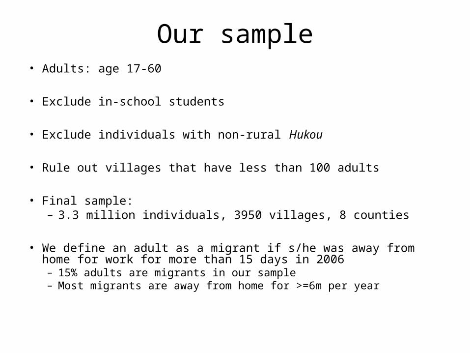
Our sample• Adults: age 17-60

• Exclude in-school students

• Exclude individuals with non-rural Hukou

• Rule out villages that have less than 100 adults

• Final sample: – 3.3 million individuals, 3950 villages, 8 counties

• We define an adult as a migrant if s/he was away from home for work for more than 15 days in 2006– 15% adults are migrants in our sample– Most migrants are away from home for >=6m per year

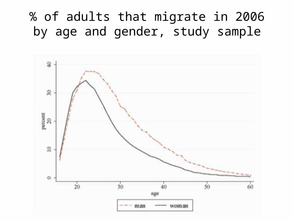
% of adults that migrate in 2006by age and gender, study sample

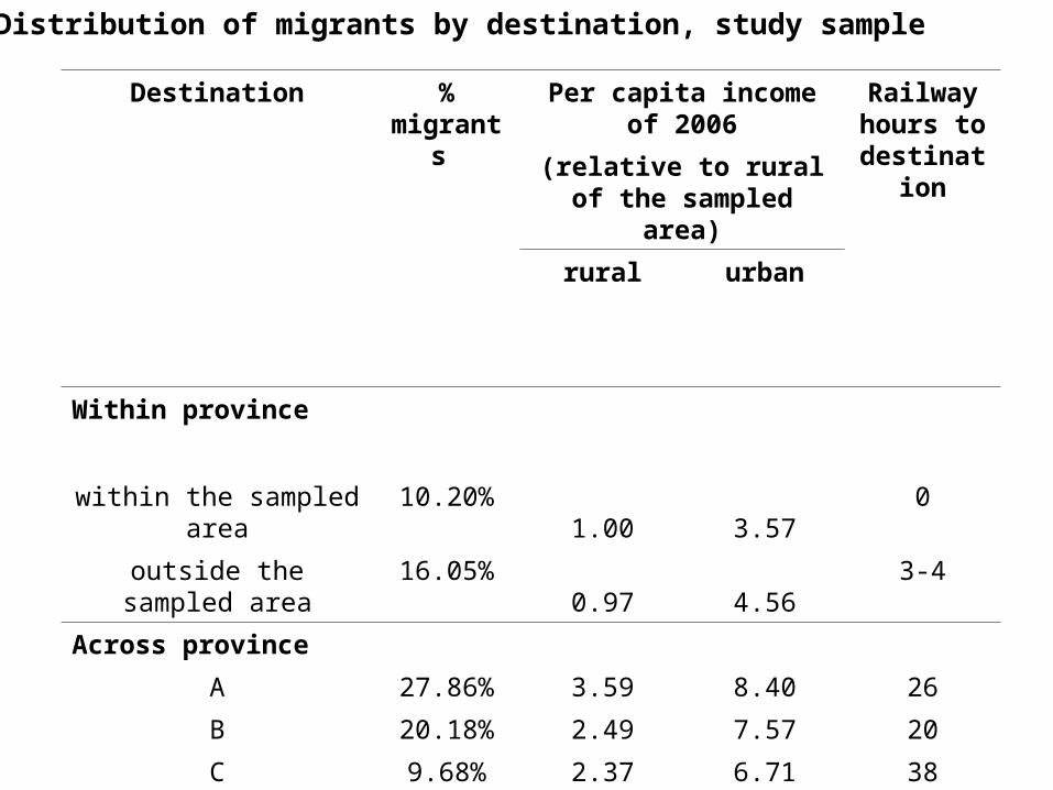
Distribution of migrants by destination, study sample

Destination % migrants

Per capita income of 2006 Railway hours to

destination(relative to rural of the

sampled area)

rural urban

Within province

within the sampled area 10.20% 1.00 3.57 0

outside the sampled area 16.05% 0.97 4.56 3-4

Across province

A 27.86% 3.59 8.40 26

B 20.18% 2.49 7.57 20

C 9.68% 2.37 6.71 38

D 4.85% 1.10 5.07 10.5

E 3.53% 2.85 6.83 36

F 1.92% 4.47 10.98 26.5

G 0.20% 1.41 5.57 6.5

H 0.63% 1.47 4.51 13

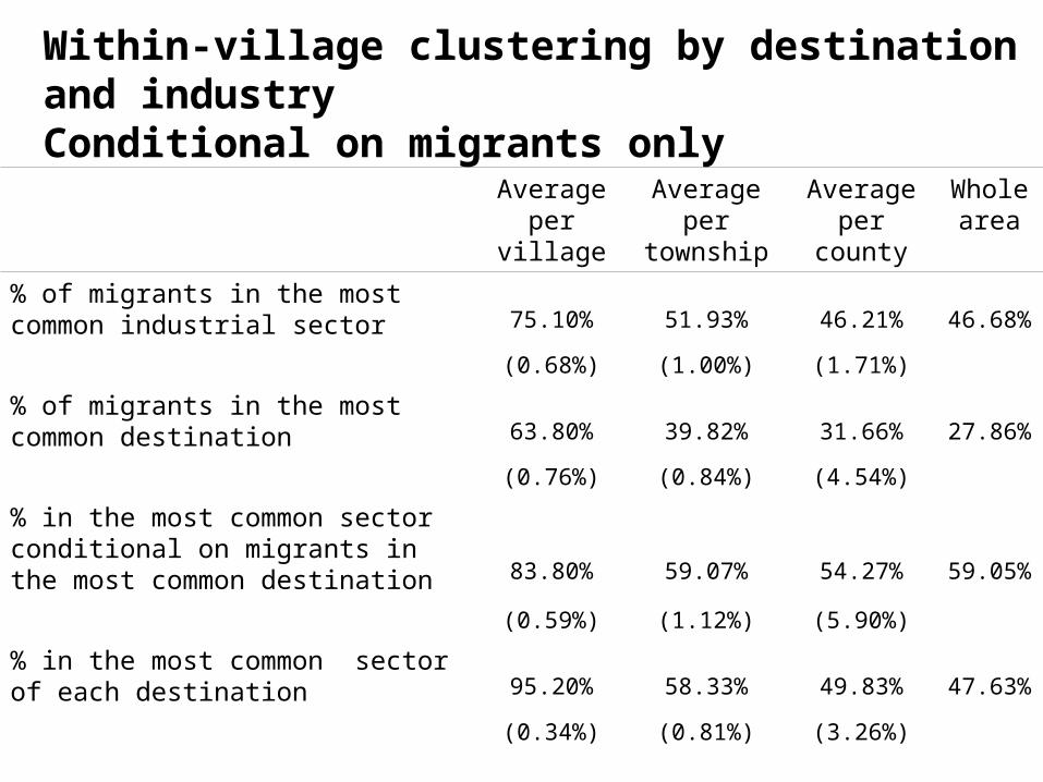
Within-village clustering by destination and industryConditional on migrants only

　 Average per village

Average per township

Average per county

Whole area

% of migrants in the most common industrial sector 75.10% 51.93% 46.21% 46.68%

(0.68%) (1.00%) (1.71%)

% of migrants in the most common destination 63.80% 39.82% 31.66% 27.86%

(0.76%) (0.84%) (4.54%)

% in the most common sector conditional on migrants in the most common destination 83.80% 59.07% 54.27% 59.05%

(0.59%) (1.12%) (5.90%)

% in the most common sector of each destination 95.20% 58.33% 49.83% 47.63%

(0.34%) (0.81%) (3.26%)

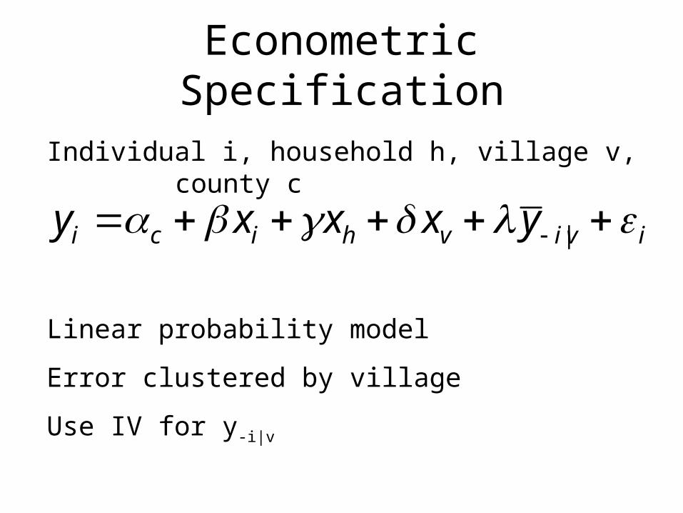
Econometric Specification

|i c i h v i v iy x x x y

Individual i, household h, village v, county c

Linear probability model

Error clustered by village

Use IV for y-i|v

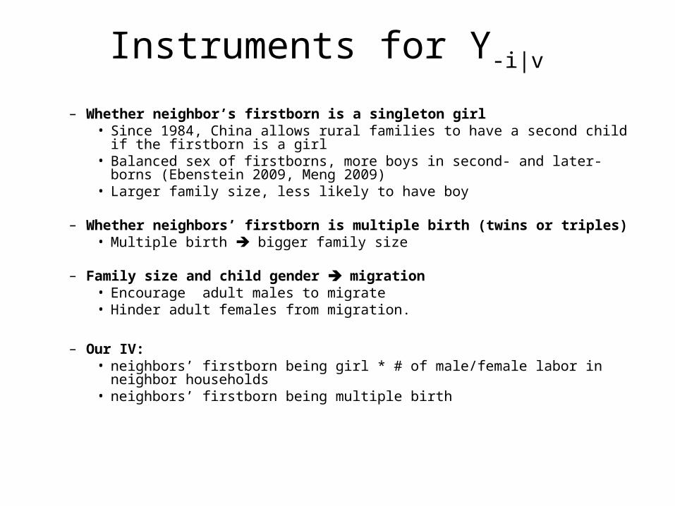
Instruments for Y-i|v

– Whether neighbor’s firstborn is a singleton girl• Since 1984, China allows rural families to have a second child if the firstborn

is a girl• Balanced sex of firstborns, more boys in second- and later-borns (Ebenstein

2009, Meng 2009)• Larger family size, less likely to have boy

– Whether neighbors’ firstborn is multiple birth (twins or triples)• Multiple birth bigger family size

– Family size and child gender migration• Encourage adult males to migrate • Hinder adult females from migration.

– Our IV: • neighbors’ firstborn being girl * # of male/female labor in neighbor

households• neighbors’ firstborn being multiple birth

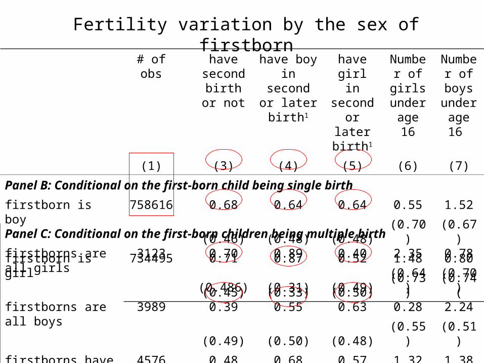
  # of obs have second birth or

not

have boy in second or later birth1

have girl in second or later birth1

Number of girls under age 16

Number of boys under

age 16

  (1) (3) (4) (5) (6) (7)

Panel B: Conditional on the first-born child being single birth

firstborn is boy 758616 0.68 0.64 0.64 0.55 1.52

(0.46) (0.48) (0.48) (0.70) (0.67)

firstborn is girl 734495 0.71 0.87 0.52 1.48 0.80

  (0.45) (0.33) (0.50) (0.73) (0.74(Panel C: Conditional on the first-born children being multiple birth

firstborns are all girls 3123 0.70 0.89 0.40 2.35 0.78

(0.486) (0.31) (0.49) (0.64) (0.70)

firstborns are all boys 3989 0.39 0.55 0.63 0.28 2.24

(0.49) (0.50) (0.48) (0.55) (0.51)

firstborns have mixed gender

4576 0.48 0.68 0.57 1.32 1.38

  (0.50) (0.46) (0.49) (0.59) (0.56)

Fertility variation by the sex of firstborn

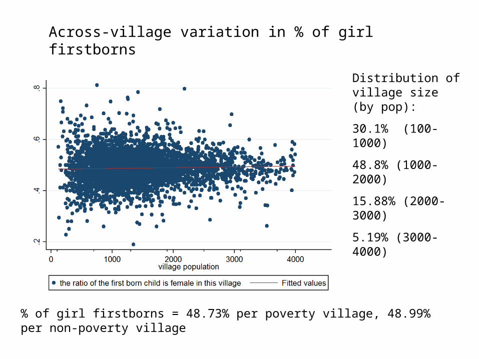
Across-village variation in % of girl firstborns

Distribution of village size (by pop):

30.1% (100-1000)

48.8% (1000-2000)

15.88% (2000-3000)

5.19% (3000-4000)

% of girl firstborns = 48.73% per poverty village, 48.99% per non-poverty village

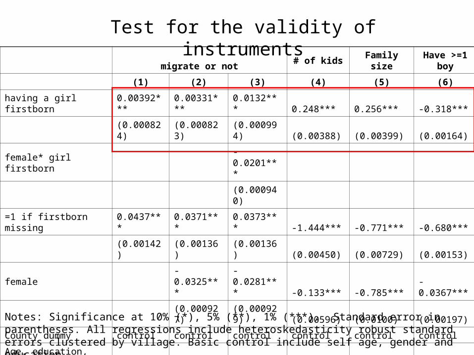
Notes: Significance at 10% (*), 5% (**), 1% (***). Standard error in parentheses. All regressions include heteroskedasticity robust standard errors clustered by village. Basic control include self age, gender and education.

Test for the validity of instruments

migrate or not# of kids Family size

Have >=1 boy

(1) (2) (3) (4) (5) (6)

having a girl firstborn 0.00392*** 0.00331*** 0.0132*** 0.248*** 0.256*** -0.318***

(0.000824) (0.000823) (0.000994) (0.00388) (0.00399) (0.00164)

female* girl firstborn -0.0201***

(0.000940)

=1 if firstborn missing 0.0437*** 0.0371*** 0.0373*** -1.444*** -0.771*** -0.680***

(0.00142) (0.00136) (0.00136) (0.00450) (0.00729) (0.00153)

female -0.0325*** -0.0281*** -0.133*** -0.785*** -0.0367***

(0.000927) (0.000929) (0.00596) (0.0100) (0.00197)

County dummy control control control control control control

Age, education,distance to station

No Yes Yes Yes Yes Yes

Observations 3,327,996 3,327,996 3,327,996 1,153,804 1,153,804 1,153,804

Level of Observations individual individual individual household household household

R square 0.0879 0.2016 0.2017 0.5298 0.1986 0.4667

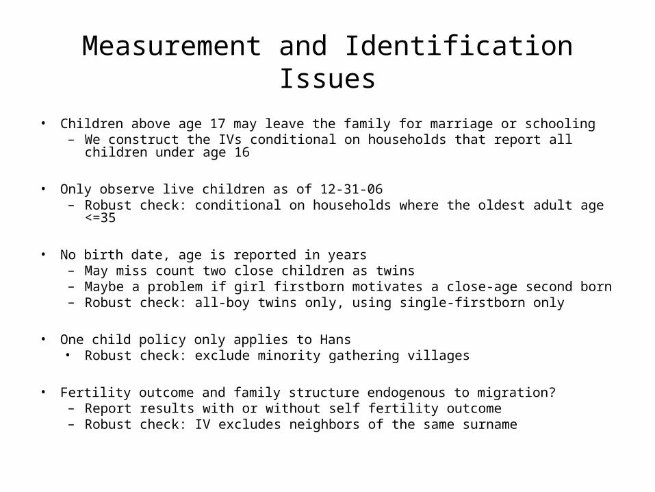
Measurement and Identification Issues

• Children above age 17 may leave the family for marriage or schooling– We construct the IVs conditional on households that report all children under

age 16

• Only observe live children as of 12-31-06– Robust check: conditional on households where the oldest adult age <=35

• No birth date, age is reported in years – May miss count two close children as twins– Maybe a problem if girl firstborn motivates a close-age second born– Robust check: all-boy twins only, using single-firstborn only

• One child policy only applies to Hans• Robust check: exclude minority gathering villages

• Fertility outcome and family structure endogenous to migration?– Report results with or without self fertility outcome– Robust check: IV excludes neighbors of the same surname

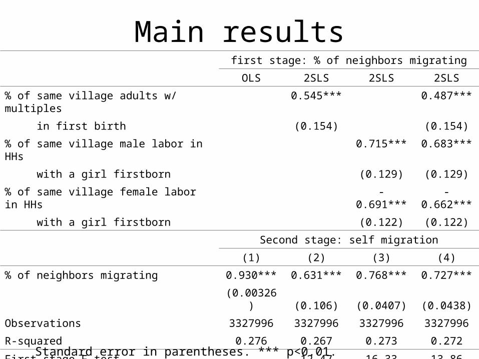
Main results

iy

Standard error in parentheses. *** p<0.01.

first stage: % of neighbors migrating

OLS 2SLS 2SLS 2SLS

% of same village adults w/ multiples 0.545*** 0.487***

in first birth (0.154) (0.154)

% of same village male labor in HHs 0.715*** 0.683***

with a girl firstborn (0.129) (0.129)

% of same village female labor in HHs -0.691*** -0.662***

with a girl firstborn (0.122) (0.122)

　 Second stage: self migration

(1) (2) (3) (4)

% of neighbors migrating 0.930*** 0.631*** 0.768*** 0.727***

(0.00326) (0.106) (0.0407) (0.0438)

Observations 3327996 3327996 3327996 3327996

R-squared 0.276 0.267 0.273 0.272

First stage F test 12.47 16.33 13.86

Weak IV test (conditional LR) [0.57,0.67] [0.72,0.79] [0.69,0.74]

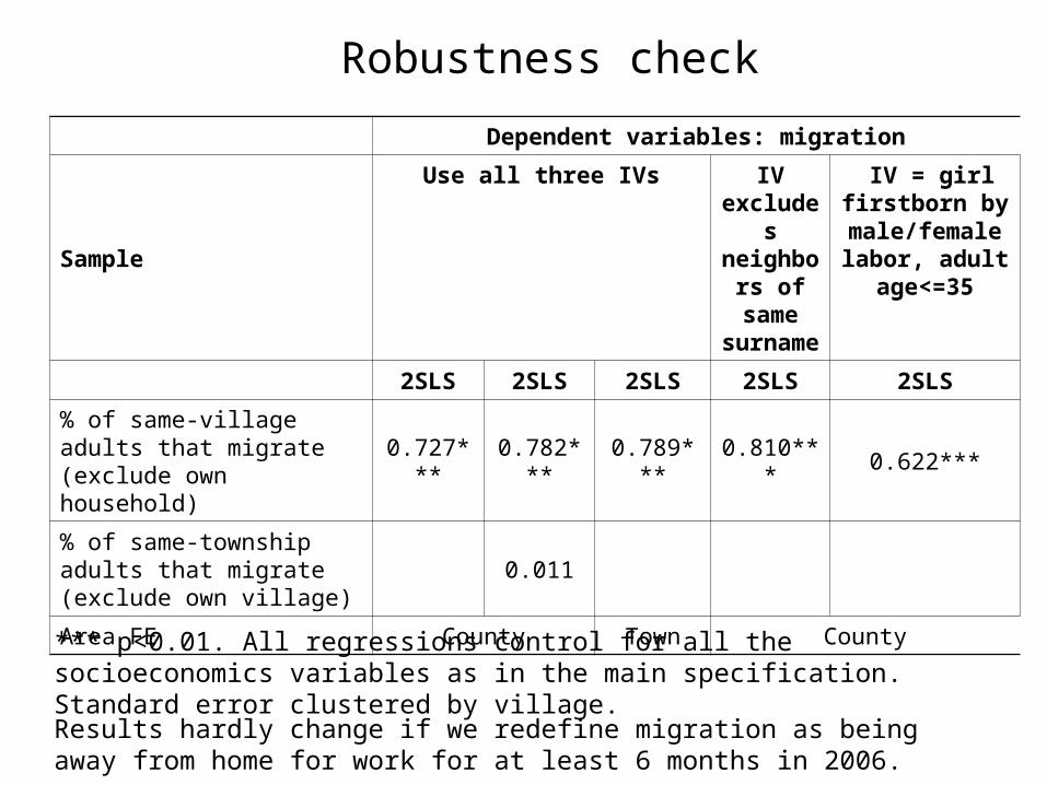
Dependent variables: migration

Sample

Use all three IVs IV excludes

neighbors of same surname

IV = girl firstborn by male/female labor, adult

age<=35

2SLS 2SLS 2SLS 2SLS 2SLS

% of same-village adults that migrate (exclude own household)

0.727*** 0.782*** 0.789*** 0.810*** 0.622***

% of same-township adults that migrate (exclude own village)

0.011

Area FE County Town County

Robustness check

Results hardly change if we redefine migration as being away from home for work for at least 6 months in 2006.

*** p<0.01. All regressions control for all the socioeconomics variables as in the main specification. Standard error clustered by village.

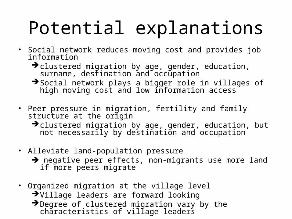
Potential explanations• Social network reduces moving cost and provides job information

clustered migration by age, gender, education, surname, destination and occupation

Social network plays a bigger role in villages of high moving cost and low information access

• Peer pressure in migration, fertility and family structure at the originclustered migration by age, gender, education, but not

necessarily by destination and occupation

• Alleviate land-population pressure negative peer effects, non-migrants use more land if more peers

migrate

• Organized migration at the village levelVillage leaders are forward lookingDegree of clustered migration vary by the characteristics of

village leaders

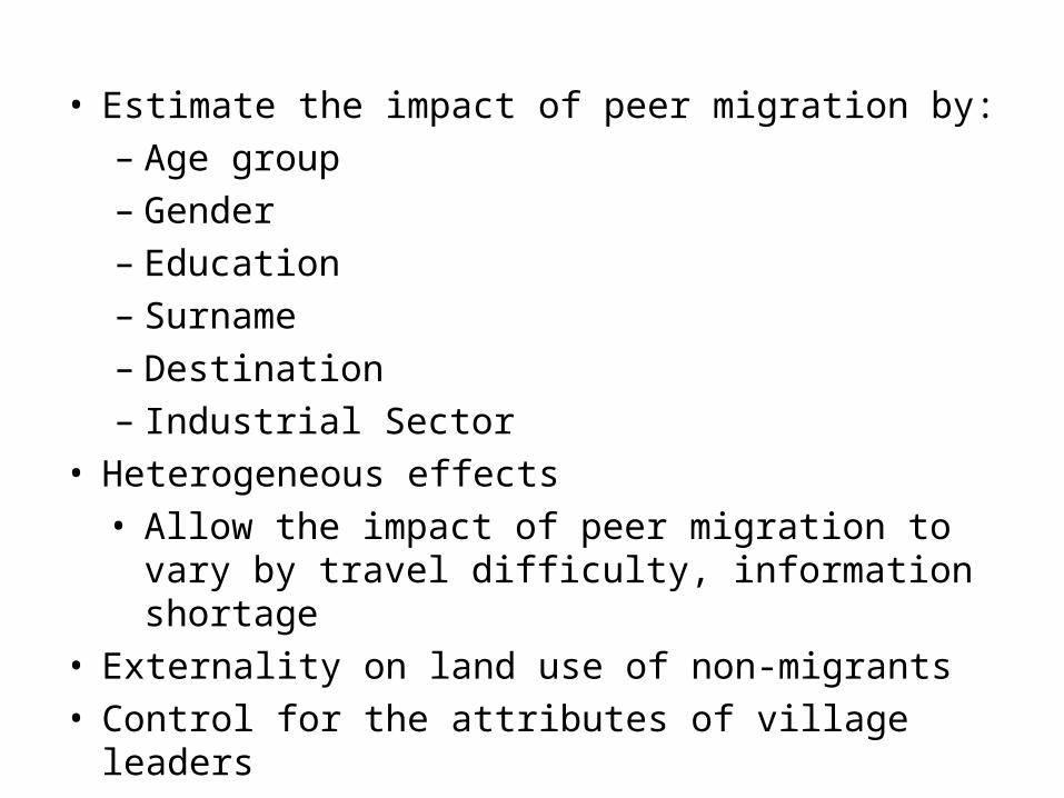
• Estimate the impact of peer migration by:

– Age group

– Gender

– Education

– Surname

– Destination

– Industrial Sector

• Heterogeneous effects

• Allow the impact of peer migration to vary by travel difficulty, information shortage

• Externality on land use of non-migrants

• Control for the attributes of village leaders

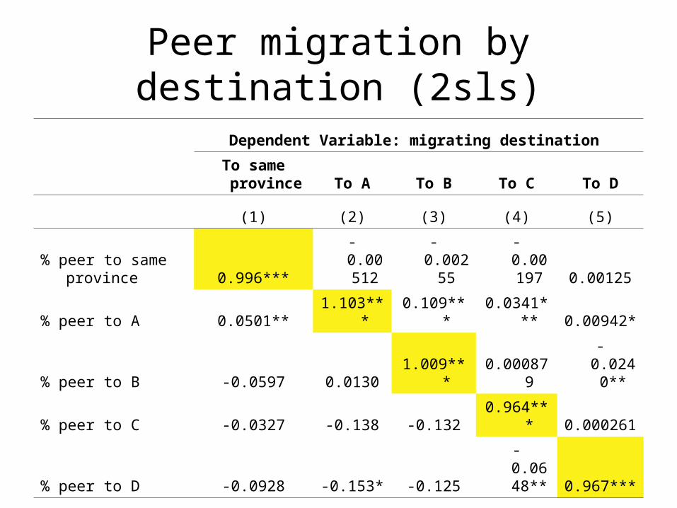
Peer migration by destination (2sls)

　 Dependent Variable: migrating destination

To same

province To A To B To C To D

　 (1) (2) (3) (4) (5)

% peer to same province 0.996*** -0.00512 -0.00255 -0.00197 0.00125

% peer to A 0.0501** 1.103*** 0.109*** 0.0341*** 0.00942*

% peer to B -0.0597 0.0130 1.009*** 0.000879 -0.0240**

% peer to C -0.0327 -0.138 -0.132 0.964*** 0.000261

% peer to D -0.0928 -0.153* -0.125 -0.0648** 0.967***

Observations 3327996 3327996 3327996 3327996 3327996

R-squared 0.102 0.106 0.097 0.068 0.043

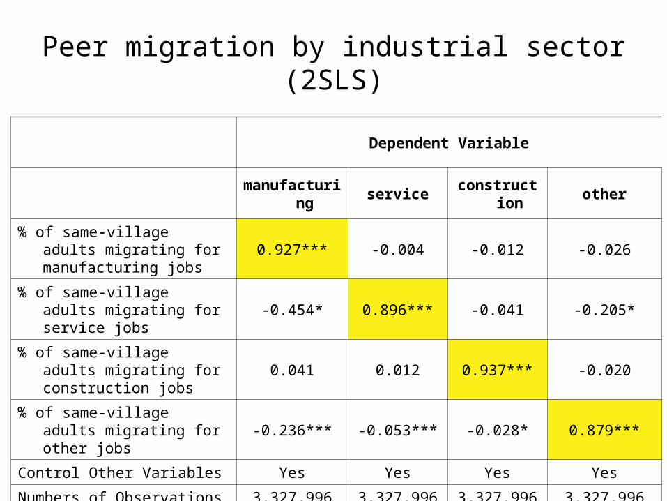
Peer migration by industrial sector (2SLS)

Dependent Variable

manufacturing service construction other

% of same-village adults migrating for manufacturing jobs

0.927*** -0.004 -0.012 -0.026

% of same-village adults migrating for service jobs

-0.454* 0.896*** -0.041 -0.205*

% of same-village adults migrating for construction jobs

0.041 0.012 0.937*** -0.020

% of same-village adults migrating for other jobs

-0.236*** -0.053*** -0.028* 0.879***

Control Other Variables Yes Yes Yes Yes

Numbers of Observations 3,327,996 3,327,996 3,327,996 3,327,996

R-squared 0.190 0.065 0.071 0.132

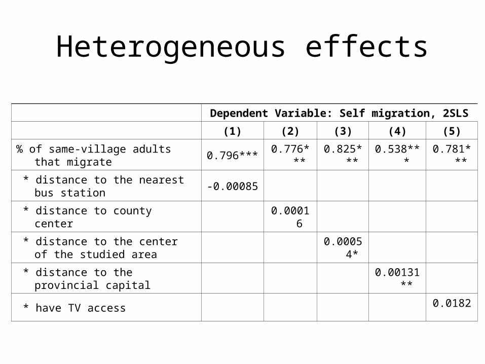
Heterogeneous effects

Dependent Variable: Self migration, 2SLS

(1) (2) (3) (4) (5)

% of same-village adults that migrate 0.796*** 0.776*** 0.825*** 0.538*** 0.781***

* distance to the nearest bus station -0.00085

* distance to county center 0.00016

* distance to the center of the studied area

0.00054*

* distance to the provincial capital 0.00131**

* have TV access 0.0182

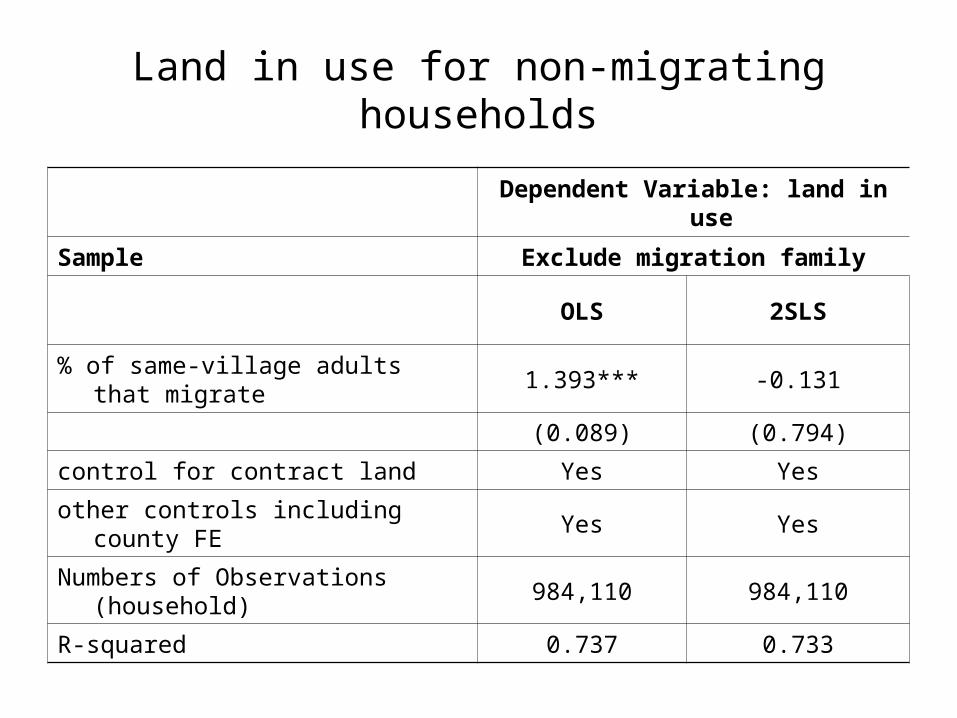
Land in use for non-migrating households

Dependent Variable: land in use

Sample Exclude migration family

OLS 2SLS

% of same-village adults that migrate 1.393*** -0.131

(0.089) (0.794)

control for contract land Yes Yes

other controls including county FE Yes Yes

Numbers of Observations (household) 984,110 984,110

R-squared 0.737 0.733

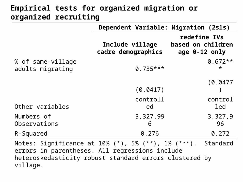
Empirical tests for organized migration or organized recruiting

  Dependent Variable: Migration (2sls)

Include village cadre demographics

redefine IVs based on children age 0-12 only

% of same-village adults migrating 0.735*** 0.672***

(0.0417) (0.0477)

Other variables controlled controlled

Numbers of Observations 3,327,996 3,327,996

R-Squared 0.276 0.272

Notes: Significance at 10% (*), 5% (**), 1% (***). Standard errors in parentheses. All regressions include heteroskedasticity robust standard errors clustered by village.

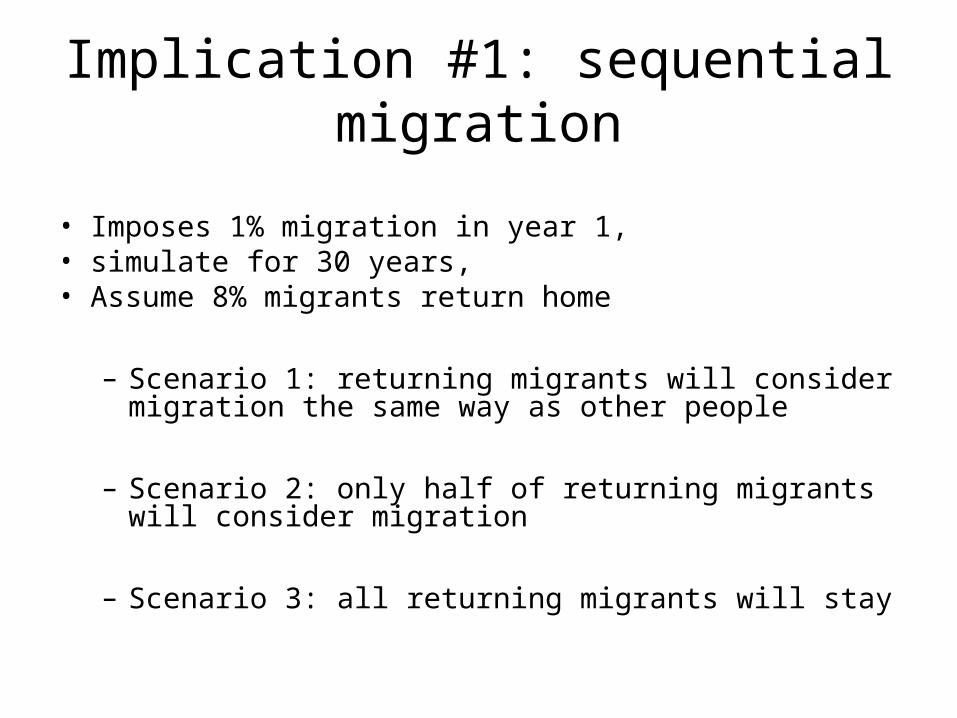
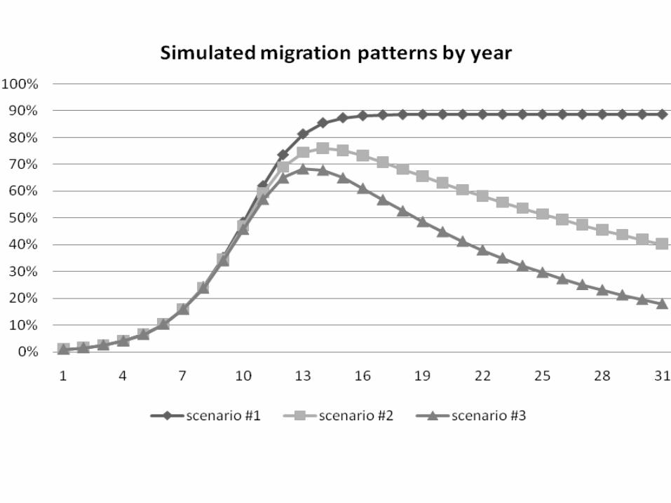
Implication #1: sequential migration

• Imposes 1% migration in year 1, • simulate for 30 years, • Assume 8% migrants return home

– Scenario 1: returning migrants will consider migration the same way as other people

– Scenario 2: only half of returning migrants will consider migration

– Scenario 3: all returning migrants will stay

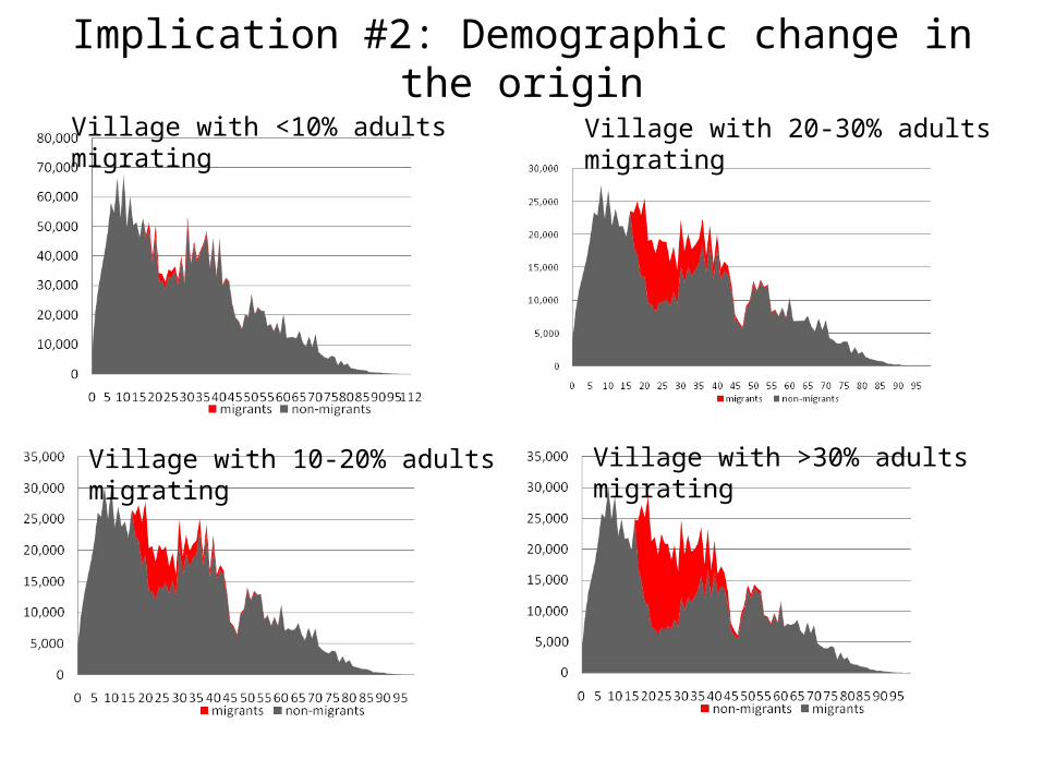
Implication #2: Demographic change in the origin

Village with <10% adults migrating

Village with 10-20% adults migrating Village with >30% adults migrating

Village with 20-30% adults migrating

Other implications• Traffic congestion

– Clustered migration aggravates the problem

• Agricultural productivity– Zero effect after using IV

• Macro vulnerability– It is estimated that 20 out of the 130+ million rural-to-urban

migrants lose or could not find job in early 2009. For a typical migrating family, income from city employment accounts for 40% of total family income

– Clustered migration establishes strong employment link between origin and destination

– Cluster migration reduces the origin’s ability to diversify unemployment risk

Conclusion• Social networks defined by rural co-villagers have large,

significant, causal effects in self migration within China

• Migration is clustered by age, gender, education, surname, destination and industrial sector

• Find evidence for many mechanisms, but the evidence is the strongest for the mechanism of social networks in reducing moving cost and providing job information

• Clustered migration has serious implications in many important areas

• Caveat: one area, cross-sectional, no data on migration history

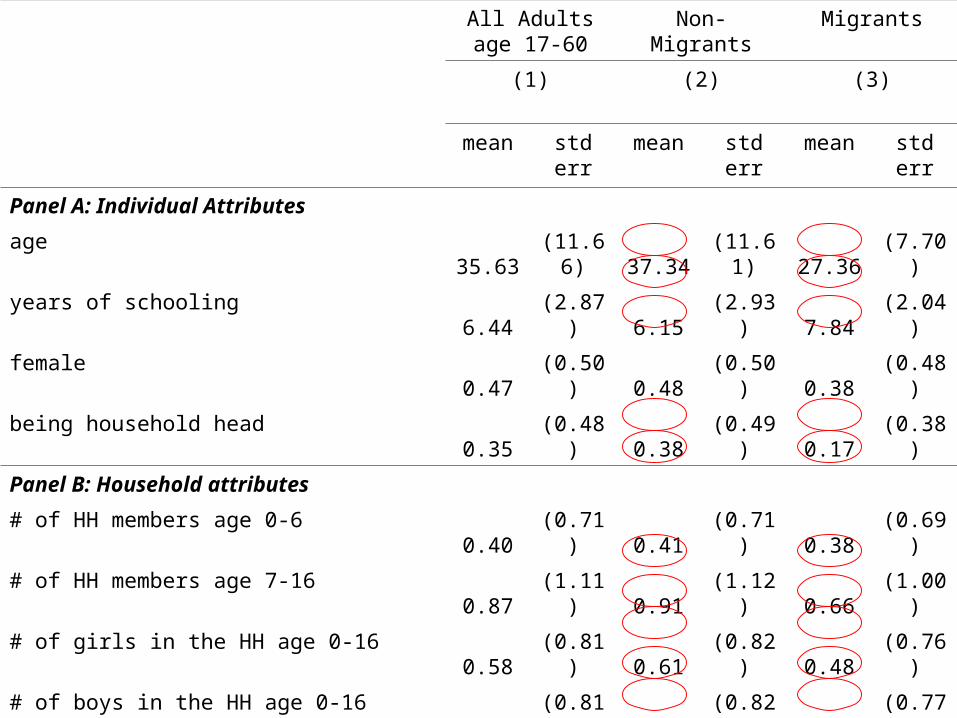
  All Adults age 17-60

Non-Migrants Migrants

(1) (2) (3)

mean std err mean std err mean std err

Panel A: Individual Attributes

age 35.63 (11.66) 37.34 (11.61) 27.36 (7.70)

years of schooling 6.44 (2.87) 6.15 (2.93) 7.84 (2.04)

female 0.47 (0.50) 0.48 (0.50) 0.38 (0.48)

being household head 0.35 (0.48) 0.38 (0.49) 0.17 (0.38)

Panel B: Household attributes

# of HH members age 0-6 0.40 (0.71) 0.41 (0.71) 0.38 (0.69)

# of HH members age 7-16 0.87 (1.11) 0.91 (1.12) 0.66 (1.00)

# of girls in the HH age 0-16 0.58 (0.81) 0.61 (0.82) 0.48 (0.76)

# of boys in the HH age 0-16 0.68 (0.81) 0.71 (0.82) 0.55 (0.77)

Has any boy in the HH? (age 0-16) 0.49 (0.50) 0.51 (0.50) 0.41 (0.49)

estimated house value (10,000 yuan) 2.36 (2.80) 2.37 (2.87) 2.28 (2.43)

have any outstanding loans 0.14 (0.34) 0.13 (0.34) 0.15 (0.36)

contract land (mu)5 3.45 (2.54) 3.44 (2.55) 3.48 (2.45)

land in use (mu)5 4.13 (3.04) 4.15 (3.04) 3.99 (3.06)