Peer-to-Peer Coordination of Autonomous Sensors inHigh-Latency Networks using

Distributed Scheduling and Data Fusion∗

Lambert Meertens and Stephen Fitzpatrick

December 2001

Kestrel Institute Technical Report KES.U.01.09Kestrel Institute, 3260 Hillview Avenue,

Palo Alto, CA 94304, USAmeertens@kestrel.edu & fitzpatrick@kestrel.edu

Project: e-Merge-ANThttp://ants.kestrel.edu/

Abstract

This report details an approach to the real-time coordination of large networks of short-range sensorsthat communicate over short-range, low-bandwidth, high-latency radio channels.

Each sensor is limited in the distance over which it can scan and in the type of data that it can acquire, sonearby sensors must collaborate to acquire complementary data for accomplishing such tasks as multiple-target detection and tracking.

Operational limitations on sensors and real-time requirements on tasks restrict the number of tasksin which a given sensor can collaborate. The quality with which a given task is accomplished and thecost incurred are affected by which particular sensors collaborate in achieving the task. Consequently, acoordination mechanism is required to optimize collaboration.

The coordination mechanism reported is fully distributed — each sensor decides for itself which mea-surements it should take to achieve optimal collaboration with nearby sensors, based what it knows abouttheir intended measurements, and informs those sensors of its own intentions so that they can likewiseoptimize their own measurements.

In order to determine which measurements are optimal, a sensor must have knowledge about the targetsthat are the intended subjects of the measurements. To this end, each sensor exchanges measurement datawith nearby sensors, and operates a data fusion process to maintain local target estimates.

The reported coordination mechanism is claimed to be scalable, low-cost, adaptive and robust.

Keywords: distributed constraint optimization, distributed scheduling, distributed resource manage-ment

∗This work is sponsored in part by DARPA through the ‘Autonomous Negotiating Teams’ program under contract #F30602-00-C-0014, monitored by the Air Force Research Laboratory. The views and conclusions contained in this document are those of the authorsand should not be interpreted as representing the official policies, either expressed or implied, of the Defense Advanced Research ProjectsAgency or the U.S. Government.

Contents

1 Introduction 1

2 Example Application: Target Tracking 2

2.1 The Sensors: Simple Active Radars . . . . . . . . . . . . . . . . . . . . . . . . . . . . . . 2

2.2 Target Tracking . . . . . . . . . . . . . . . . . . . . . . . . . . . . . . . . . . . . . . . . . 3

2.3 Broadcast Communication . . . . . . . . . . . . . . . . . . . . . . . . . . . . . . . . . . . 4

3 World Estimates and Quality Metrics 4

3.1 Trajectories . . . . . . . . . . . . . . . . . . . . . . . . . . . . . . . . . . . . . . . . . . . 6

3.2 Measurements and Sensor Models . . . . . . . . . . . . . . . . . . . . . . . . . . . . . . . 7

3.3 Data Fusion . . . . . . . . . . . . . . . . . . . . . . . . . . . . . . . . . . . . . . . . . . . 8

3.4 Coordination Mechanism . . . . . . . . . . . . . . . . . . . . . . . . . . . . . . . . . . . . 9

4 Proximate Metric 9

4.1 Proximate Metric with respect to Probability Distributions over Trajectories . . . . . . . . . 11

4.2 Quality of Measurements with respect to Single Trajectory . . . . . . . . . . . . . . . . . . 12

4.3 Measurement Feasibility . . . . . . . . . . . . . . . . . . . . . . . . . . . . . . . . . . . . 15

4.4 Overall Quality (including Operational Cost) . . . . . . . . . . . . . . . . . . . . . . . . . 16

5 Coordination Mechanism 17

5.1 Local World Estimates . . . . . . . . . . . . . . . . . . . . . . . . . . . . . . . . . . . . . 17

5.2 Local Schedules . . . . . . . . . . . . . . . . . . . . . . . . . . . . . . . . . . . . . . . . . 18

5.3 Local Schedule Quality Metrics . . . . . . . . . . . . . . . . . . . . . . . . . . . . . . . . 18

5.4 Distributed Coordination Mechanism . . . . . . . . . . . . . . . . . . . . . . . . . . . . . . 19

6 Radar Example: Further Details 21

6.1 Target Models . . . . . . . . . . . . . . . . . . . . . . . . . . . . . . . . . . . . . . . . . . 21

6.2 Schedules . . . . . . . . . . . . . . . . . . . . . . . . . . . . . . . . . . . . . . . . . . . . 22

6.3 Local Metrics . . . . . . . . . . . . . . . . . . . . . . . . . . . . . . . . . . . . . . . . . . 22

6.4 Search . . . . . . . . . . . . . . . . . . . . . . . . . . . . . . . . . . . . . . . . . . . . . . 24

7 Conclusion 25

iii

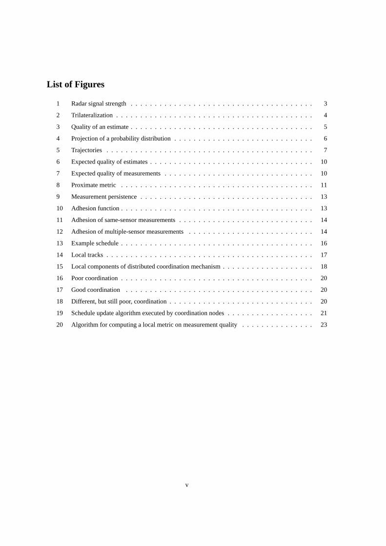
List of Figures

1 Radar signal strength . . . . . . . . . . . . . . . . . . . . . . . . . . . . . . . . . . . . . . 3

2 Trilateralization . . . . . . . . . . . . . . . . . . . . . . . . . . . . . . . . . . . . . . . . . 4

3 Quality of an estimate . . . . . . . . . . . . . . . . . . . . . . . . . . . . . . . . . . . . . . 5

4 Projection of a probability distribution . . . . . . . . . . . . . . . . . . . . . . . . . . . . . 6

5 Trajectories . . . . . . . . . . . . . . . . . . . . . . . . . . . . . . . . . . . . . . . . . . . 7

6 Expected quality of estimates . . . . . . . . . . . . . . . . . . . . . . . . . . . . . . . . . . 10

7 Expected quality of measurements . . . . . . . . . . . . . . . . . . . . . . . . . . . . . . . 10

8 Proximate metric . . . . . . . . . . . . . . . . . . . . . . . . . . . . . . . . . . . . . . . . 11

9 Measurement persistence . . . . . . . . . . . . . . . . . . . . . . . . . . . . . . . . . . . . 13

10 Adhesion function . . . . . . . . . . . . . . . . . . . . . . . . . . . . . . . . . . . . . . . . 13

11 Adhesion of same-sensor measurements . . . . . . . . . . . . . . . . . . . . . . . . . . . . 14

12 Adhesion of multiple-sensor measurements . . . . . . . . . . . . . . . . . . . . . . . . . . 14

13 Example schedule . . . . . . . . . . . . . . . . . . . . . . . . . . . . . . . . . . . . . . . . 16

14 Local tracks . . . . . . . . . . . . . . . . . . . . . . . . . . . . . . . . . . . . . . . . . . . 17

15 Local components of distributed coordination mechanism . . . . . . . . . . . . . . . . . . . 18

16 Poor coordination . . . . . . . . . . . . . . . . . . . . . . . . . . . . . . . . . . . . . . . . 20

17 Good coordination . . . . . . . . . . . . . . . . . . . . . . . . . . . . . . . . . . . . . . . 20

18 Different, but still poor, coordination . . . . . . . . . . . . . . . . . . . . . . . . . . . . . . 20

19 Schedule update algorithm executed by coordination nodes . . . . . . . . . . . . . . . . . . 21

20 Algorithm for computing a local metric on measurement quality . . . . . . . . . . . . . . . 23

v

1 Introduction

There is currently interest in using large networks of simple sensors to perform traditional sensingtasks(such as target detection and tracking) in a way that has low set-up and maintenance costs. For example, onescenario envisions the deployment of tens of thousands of small, cheap, battery-powered, short-range sensorsthat use low-power radios for communicating measurements and to coordination inter-sensor collaborationon target detection and tracking.

Inter-sensorcollaborationis required because an individual sensor may be capable of scanning only a limitedgeographical area and acquiring only partial information about a target; for example, it may be capable ofdetermining the distance from itself to the target, but not the direction. Consequently, several sensors needto collaborate to acquire complementary data that isfusedto produce complete target estimates. To ensurehigh-quality data fusion, the sensors may need to take their measurements approximately simultaneously.

The objective of the network’scoordination mechanismis to determine which sensors should collaborate andwhich measurements each should take — typically, there are many possible combinations of sensors thatcould achieve a given task (such as tracking a target) and each sensor could usefully participate in severaltasks but it is limited in the number of tasks in which it can participate at any given time. Thequality of theestimates produced by the data fusion process and thecostof achieving the given tasks (measured, e.g., interms of the energy used) can be significantly affected by the coordination decisions.

The tasks that are to be achieved by the sensor network are dynamic:

• As targets move, the set of sensors that can scan the targets changes.

• New targets are detected by background scans, giving rise to new tracking tasks.

• Tracked targets move beyond the range of the sensor network, causing a tracking task to becomeobsolete.

Moreover, the status of the sensor network is typically dynamic; e.g., hardware may fail.

As circumstances change, the sensors must re-coordinate to adapt, and coordination itself must be robustagainst hardware failure. Because there are temporal requirements on the tasks (e.g., a given target willbe within range of a given sensor for only a limited period), coordination must be achieved in real-time.Moreover, the number of sensors is expected to be high (e.g.,105) so coordination must be scalable.

Given these requirements, a highly-distributed coordination mechanism seems appropriate:

• The distance over which communication can take place in a single ‘hop’ is limited by the power ofthe radio transmitter. A distributed coordination mechanism allows most decisions to be made locally,using only single-hop communication, which in turn allows the network to adapt quickly.

• For non-trivial sensors, coordination is likely to be combinatorially hard. A distributed coordinationmechanism allows the computational costs to be spread over many computational units. The objectiveis to have a scalable coordination mechanism, in which, e.g., the number of computational units growslinearly with the number of sensors and the load on each computational unit remains fixed.

• A distributed coordination mechanism is inherently more robust against hardware failure. For example,the failure of a few computational units should not cause the failure of the entire coordination network,and hence the entire sensor network.

Of course, distributing the coordination mechanism raises it own potential problems: each component of thedistributed mechanism needs to adapt the behavior of the sensors under its control quickly enough to keepapace with changes in target number and/or behavior, but each component must also have regard for the ac-tions being performed by nearby sensors (under the control of other coordination components) in order to

1

ensure high quality collaboration between the sensors. That is, there is a need to balance speed of adapta-tion against ‘coherence’ of decisions made by autonomous but interacting components of the coordinationmechanism.

The remainder of this report describes a highly-distributed coordination mechanism in which each sensor hasits own coordination component, which interacts with other coordination components using a peer-to-peer,stochastic, hill-climbing optimization algorithm. An example involving simple radar sensors is given.

The structure of the remainder of this report is as follows:

• The radar sensor hardware is described along with some details of the communication infrastructure.

• The problem to be solved is defined in terms of the quality of target tracking that is expected to arisefrom a proposed vector of measurements, given current target tracks, models of target behavior and sen-sor models. It is argued that coordinating sensors based directly on this criterion is too computationallyexpensive for real-time systems.

• An alternative problem is introduced: optimizing the expected quality of sensing. Although sensingquality is, in this report, only heuristically related to track quality, it is conjectured that attaining high-quality sensing should lead to high-quality target tracks.

• A distributed coordination mechanism is then introduced that uses local information and local sensorinteraction to approximately solve the problem of optimizing sensing quality.

• The main details of implementing the coordination mechanism for the radar example are given.

2 Example Application: Target Tracking using Simple Radars & Lo-cal Broadcast Communication

The distributed coordination mechanism reported here is intended to be mostly generic or at least readilyadaptable to various types of sensors. Nevertheless, some design decisions are motivated by a particularapplication, involving simple radar sensors detecting and tracking standardized targets moving in a plane.This section describes the hardware and communication infrastructure, and some preliminary details aboutwhat measurements are needed for target tracking.

2.1 The Sensors: Simple Active Radars

The sensors are fixed-frequency, continuous-wave radars. A single sensor is comprised of three emitter-detector pairs and one sampler (an analogue-to-digital converter). Each detector can receive only the signalfrom its corresponding emitter after reflection off a target. At any given time, the sampler can measure thestrength of the radar signal received by one and only one of the detectors. For a single measurement, thesampler is used in one of two possible modes:

• in amplitude-only mode, the sampler reports the maximum signal amplitude measured over a period ofapproximately 0.6 seconds;

• in amplitude-and-frequency mode, the sampler reports both the maximum signal amplitude measuredand the Doppler shift between the emitted and reflected signals; the time required for this mode dependson the Doppler frequency and varies between approximately 0.6 and 1.8 seconds.

2

Remitter/detector 2

mid-beam

emitter/detector 3mid-beam

emitter/detector 1 mid-beam

Target

Sensorθ

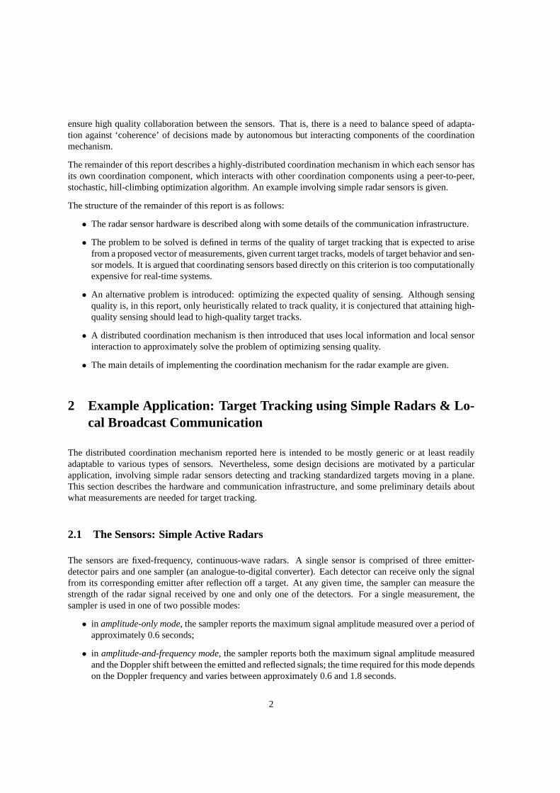
Figure 1: Signal strength detected by a radar depends on emitter-target distance and angle

The signal’s amplitude corresponds to a set of target positions, as follows. The emitter-detector pairs areoriented at 120o intervals in the plane (see Figure 1). The signal produced by an emitter is predominantlydirected forward, along the emitter’smid-beam: the signal strength expected to be detected from astandardtarget is modeled by the equation

m(R, θ) = Ke−(θ/A)2/R2 (1)

whereR is the sensor-target distance,θ is the angle between the emitter’s mid-beam and the target (0o ≤ θ ≤180o), andK andA are constants.

The emitters, detectors and sampler are subject to random noise (both internal and environmental) that limitsthe effective range of the sensors. The constantA is about 40o so that, for example, a target that is at mid-beam will produce a signal that ise9/4 ≈ 9.5 times larger than a target that is at the same distance from thesensor but that is 60o off mid-beam.

If a radar beam reflects off several targets simultaneously, the reading produced by the detector is essentiallya random combination of what the individual targets would produce separately, and is effectively useless.

The measured signal’s frequency is Doppler shifted by an amount that is directly proportional to the target’sradial speed.

Each emitter can be independently activated or deactivated. While an emitter is active, it consumes power,regardless of whether or not its detector is being sampled. If a deactivated emitter is activated, the emittedbeam is unstable and does not give reliable measurements for approximately 2 seconds.

2.2 Target Tracking

The measurements taken by a single sensor are sufficient to allow target detection (the presence of a targetnearby is indicated by a strong signal) but they are not sufficient to allow a target to be tracked: for example,a given signal amplitude indicates only that a target is at some point along a contour in the plane — it doesnot indicate where on the contour.

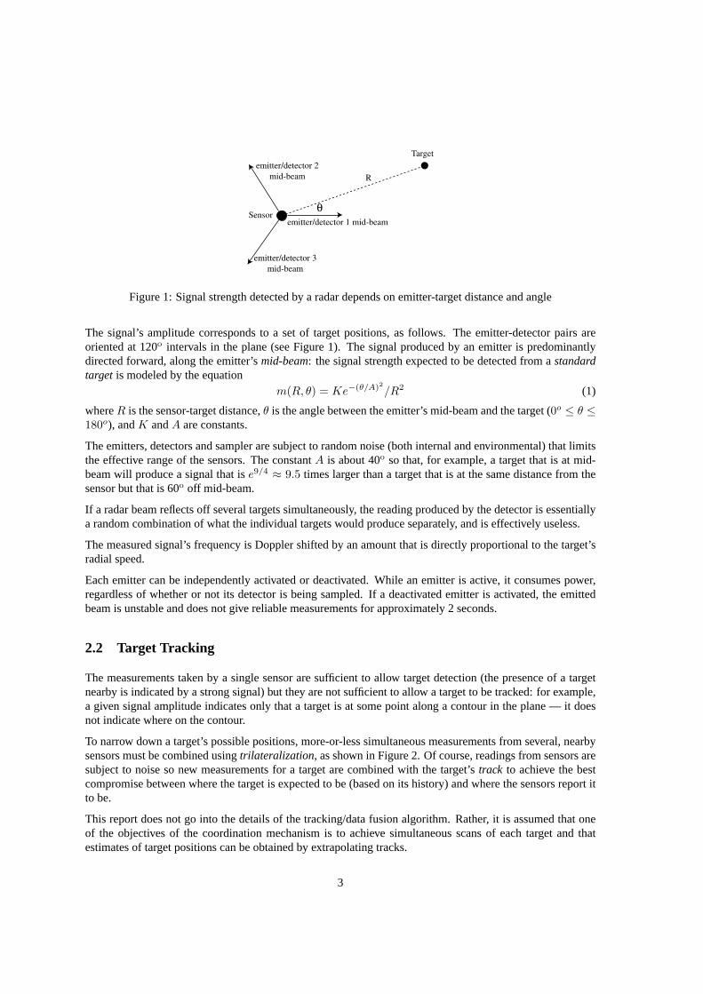
To narrow down a target’s possible positions, more-or-less simultaneous measurements from several, nearbysensors must be combined usingtrilateralization, as shown in Figure 2. Of course, readings from sensors aresubject to noise so new measurements for a target are combined with the target’strack to achieve the bestcompromise between where the target is expected to be (based on its history) and where the sensors report itto be.

This report does not go into the details of the tracking/data fusion algorithm. Rather, it is assumed that oneof the objectives of the coordination mechanism is to achieve simultaneous scans of each target and thatestimates of target positions can be obtained by extrapolating tracks.

3

TargetEstimate

Measurement Contours

Figure 2: Determining a target’s position using trilateralization

2.3 Broadcast Communication

Each radar sensor has a radio transmitter and receiver that can be used to communicate measurements and ar-bitrary data in short bursts (message lengths should preferably be kept below 100 bytes). In the demonstrationapplication, communication operates on a fixed frequency in broadcast mode on a fixed, cyclic schedule: thatis, in every cycle of the schedule, each sensor has a fixed time period during which it can transmit without in-terfering with other transmissions. The communication range is limited by the effective physical transmissionrange, so ‘broadcast’ mode is really a dense, local, multicast mode.

The number of sensors that are within communication range (and thus that are capable of interfering witheach other’s transmissions) is likely to be high relative to the number of messages that can be sent per second(the minimum duration of a message is determined by the likely size of messages and the communicationbandwidth and latency). Consequently, the period of the communication schedule, and thus the average timebetween a sensor determining that it has information to send and being able to send it, is likely to be large.

In other words, communication is likely to have higheffectivelatency even if the underlying communicationfabric’s latency is only moderate. This is expected to be true even if other, scalable communication schemesare used. High-latency communication is an underlying assumption of the rationale for the coordinationmechanism reported here.

Two final issues should be noted in passing: (1) transmission interferes with sampling, so the communicationand sensing schedules need to be compatible; (2) execution of the communication schedule is achieved au-tonomously by each sensor based on its local clock (which is synchronized with other sensors’ clocks using asimple, distributed protocol whose communication piggy-backs on transmissions for measurements and otherdata).

3 World Estimates and Quality Metrics

The objective of a sensor network is to cost-effectively maintain an estimate of certain properties of the realworld. For example, for a single target, a network’s estimate may include the target’s position, velocity,acceleration, facing (i.e., orientation relative to velocity), etc. The cost of operating the network may bemeasured as the amount of battery energy consumed, for example.

The following assumption is made:

Assumption 1 (Separable targets)A world state is a finite map from some uninterpreted domain oftargetsto single-target information.In other words, the world is assumed to be made up of separately identifiable targets, for each of which

4

S1

S2

S3 S1

S2

S3

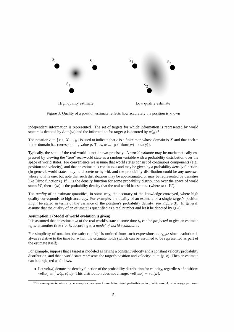
High quality estimate Low quality estimate

Figure 3: Quality of a position estimate reflects how accurately the position is known

independent information is represented. The set of targets for which information is represented by worldstatew is denoted bydom(w) and the information for targetg is denoted byw(g).1

The notatione ≡ x ∈ X → y is used to indicate thate is a finite map whose domain isX and that eachxin the domain has corresponding valuey. Thus,w ≡ g ∈ dom(w) → w(g).

Typically, the state of the real world is not known precisely. Aworld estimatemay be mathematically ex-pressed by viewing the “true” real-world state as a random variable with a probability distribution over thespace of world states. For convenience we assume that world states consist of continuous components (e.g.,position and velocity), and that an estimate is continuous and may be given by a probabilitydensityfunction.(In general, world states may be discrete or hybrid, and the probability distribution could be anymeasurewhose total is one, but note that such distributions may be approximated or may be represented by densitieslike Dirac functions.) Ifω is the density function for some probability distribution over the space of worldstatesW , thenω(w) is the probability density that the real world has statew (wherew ∈W ).

The quality of an estimate quantifies, in some way, the accuracy of the knowledge conveyed, where highquality corresponds to high accuracy. For example, the quality of an estimate of a single target’s positionmight be stated in terms of the variance of the position’s probability density (see Figure 3). In general,assume that the quality of an estimate is quantified as a real number and let it be denoted byζ(ω).

Assumption 2 (Model of world evolution is given)It is assumed that an estimateω of the real world’s state at some timet0 can beprojectedto give an estimateεt0tω at another timet > t0 according to amodel of world evolutionε.

For simplicity of notation, the subscript ‘t0’ is omitted from such expressions asεt0tω since evolution isalways relative to the time for which the estimate holds (which can be assumed to be represented as part ofthe estimate itself).

For example, suppose that a target is modeled as having a constant velocity and a constant velocity probabilitydistribution, and that a world state represents the target’s position and velocity:w ≡ 〈p, v〉. Then an estimatecan be projected as follows.

• Letvel(ω) denote the density function of the probability distribution for velocity, regardless of position:vel(ω) ≡

∫ω〈p, v〉 dp. This distribution does not change:vel(εtω) = vel(ω).

1This assumption is not strictly necessary for the abstract formulation developed in this section, but it is useful for pedagogic purposes.

5

v

p

ω

v

p

ω

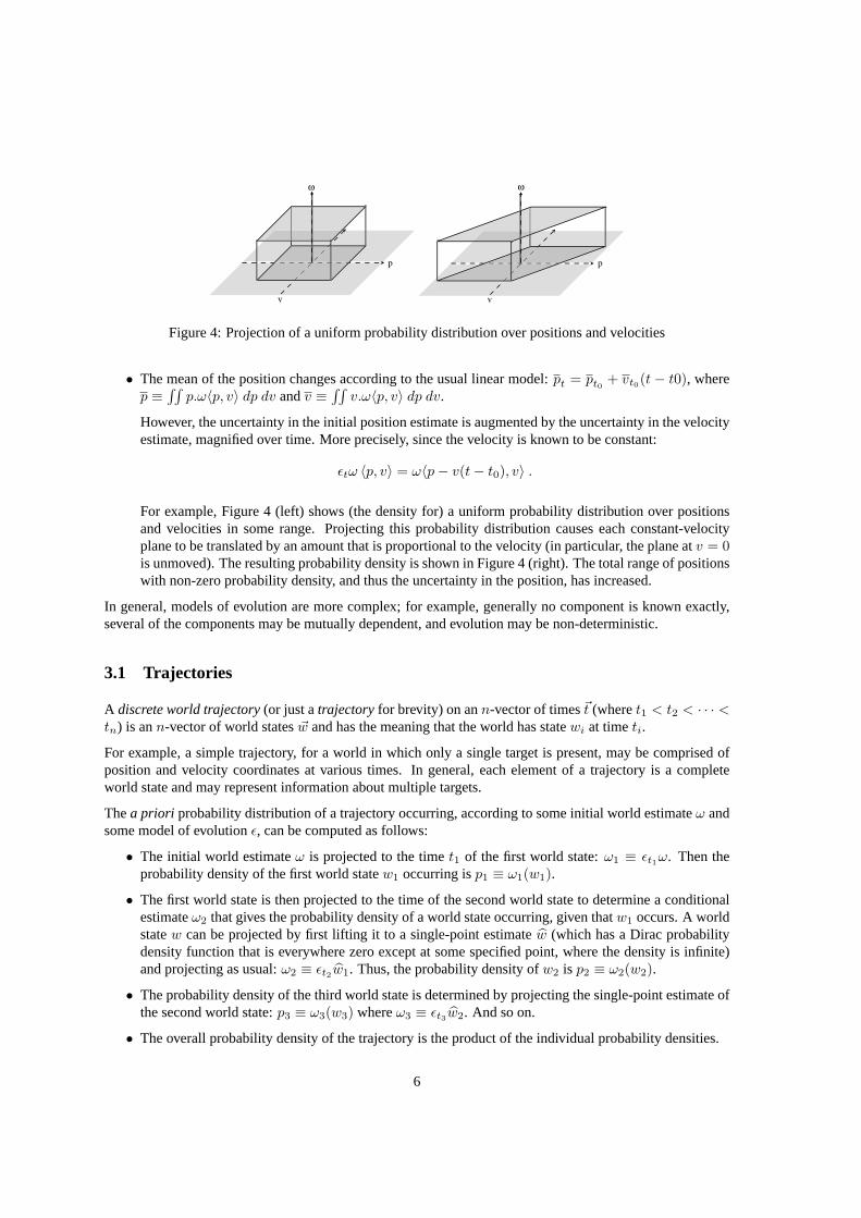
Figure 4: Projection of a uniform probability distribution over positions and velocities

• The mean of the position changes according to the usual linear model:pt = pt0 + vt0(t − t0), wherep ≡

∫∫p.ω〈p, v〉 dp dv andv ≡

∫∫v.ω〈p, v〉 dp dv.

However, the uncertainty in the initial position estimate is augmented by the uncertainty in the velocityestimate, magnified over time. More precisely, since the velocity is known to be constant:

εtω 〈p, v〉 = ω〈p− v(t− t0), v〉 .

For example, Figure 4 (left) shows (the density for) a uniform probability distribution over positionsand velocities in some range. Projecting this probability distribution causes each constant-velocityplane to be translated by an amount that is proportional to the velocity (in particular, the plane atv = 0is unmoved). The resulting probability density is shown in Figure 4 (right). The total range of positionswith non-zero probability density, and thus the uncertainty in the position, has increased.

In general, models of evolution are more complex; for example, generally no component is known exactly,several of the components may be mutually dependent, and evolution may be non-deterministic.

3.1 Trajectories

A discrete world trajectory(or just atrajectoryfor brevity) on ann-vector of times~t (wheret1 < t2 < · · · <tn) is ann-vector of world states~w and has the meaning that the world has statewi at timeti.

For example, a simple trajectory, for a world in which only a single target is present, may be comprised ofposition and velocity coordinates at various times. In general, each element of a trajectory is a completeworld state and may represent information about multiple targets.

Thea priori probability distribution of a trajectory occurring, according to some initial world estimateω andsome model of evolutionε, can be computed as follows:

• The initial world estimateω is projected to the timet1 of the first world state:ω1 ≡ εt1ω. Then theprobability density of the first world statew1 occurring isp1 ≡ ω1(w1).

• The first world state is then projected to the time of the second world state to determine a conditionalestimateω2 that gives the probability density of a world state occurring, given thatw1 occurs. A worldstatew can be projected by first lifting it to a single-point estimatew (which has a Dirac probabilitydensity function that is everywhere zero except at some specified point, where the density is infinite)and projecting as usual:ω2 ≡ εt2w1. Thus, the probability density ofw2 is p2 ≡ ω2(w2).

• The probability density of the third world state is determined by projecting the single-point estimate ofthe second world state:p3 ≡ ω3(w3) whereω3 ≡ εt3w2. And so on.

• The overall probability density of the trajectory is the product of the individual probability densities.

6

A B C

E F

D0.5

0.5

0.8

0.2

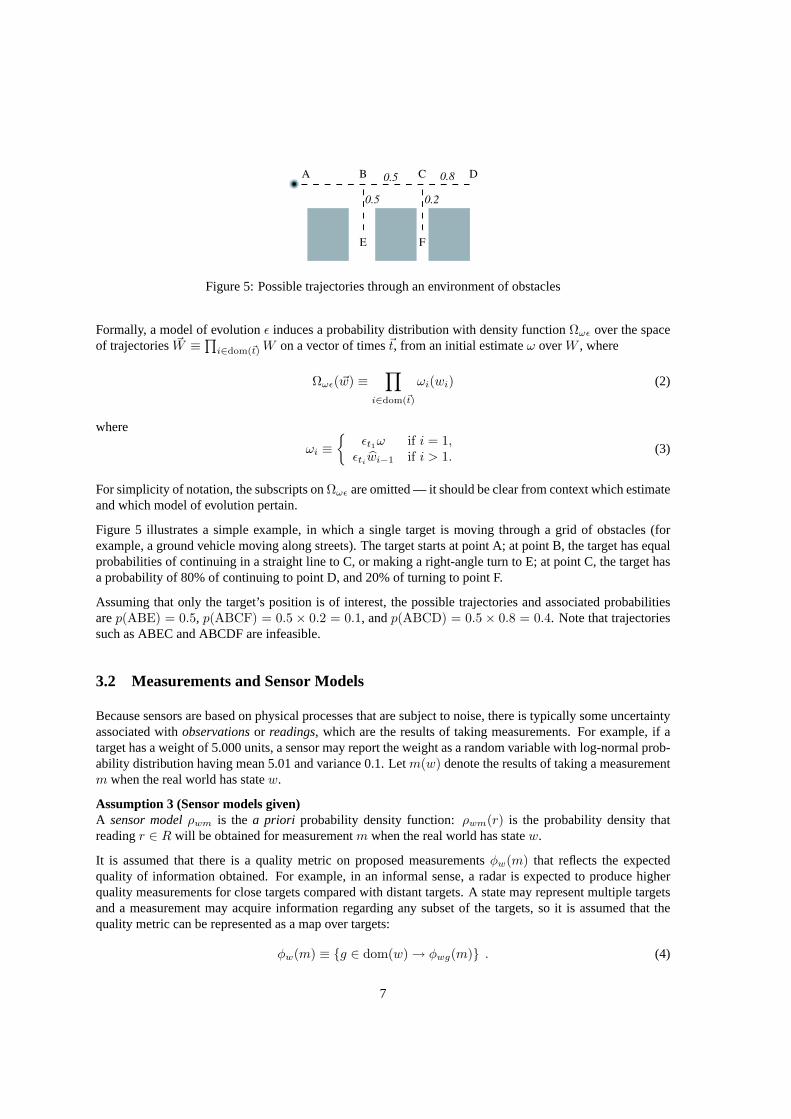
Figure 5: Possible trajectories through an environment of obstacles

Formally, a model of evolutionε induces a probability distribution with density functionΩωε over the spaceof trajectories~W ≡

∏i∈dom(~t)W on a vector of times~t, from an initial estimateω overW , where

Ωωε(~w) ≡∏

i∈dom(~t)

ωi(wi) (2)

where

ωi ≡

εt1ω if i = 1,εtiwi−1 if i > 1. (3)

For simplicity of notation, the subscripts onΩωε are omitted — it should be clear from context which estimateand which model of evolution pertain.

Figure 5 illustrates a simple example, in which a single target is moving through a grid of obstacles (forexample, a ground vehicle moving along streets). The target starts at point A; at point B, the target has equalprobabilities of continuing in a straight line to C, or making a right-angle turn to E; at point C, the target hasa probability of 80% of continuing to point D, and 20% of turning to point F.

Assuming that only the target’s position is of interest, the possible trajectories and associated probabilitiesarep(ABE) = 0.5, p(ABCF) = 0.5× 0.2 = 0.1, andp(ABCD) = 0.5× 0.8 = 0.4. Note that trajectoriessuch as ABEC and ABCDF are infeasible.

3.2 Measurements and Sensor Models

Because sensors are based on physical processes that are subject to noise, there is typically some uncertaintyassociated withobservationsor readings, which are the results of taking measurements. For example, if atarget has a weight of 5.000 units, a sensor may report the weight as a random variable with log-normal prob-ability distribution having mean 5.01 and variance 0.1. Letm(w) denote the results of taking a measurementm when the real world has statew.

Assumption 3 (Sensor models given)A sensor modelρwm is the a priori probability density function:ρwm(r) is the probability density thatreadingr ∈ R will be obtained for measurementm when the real world has statew.

It is assumed that there is a quality metric on proposed measurementsφw(m) that reflects the expectedquality of information obtained. For example, in an informal sense, a radar is expected to produce higherquality measurements for close targets compared with distant targets. A state may represent multiple targetsand a measurement may acquire information regarding any subset of the targets, so it is assumed that thequality metric can be represented as a map over targets:

φw(m) ≡ g ∈ dom(w) → φwg(m) . (4)

7

For the radar example, the basis of the measurement quality metricfor a single targetis Equation 1 whichpredicts how strong a signal should be obtained from a target. However, the quality metric should probablynot bedirectlyproportional to the signal strength: an example is given in Equation 13.

When multiple targets are present, interference may occur; i.e., the readings acquired by a sensor may notbe a simple union of the readings that would be received for each target if it alone were present. A simpleexample of interference is one target blocking another target from the view of a line-of-sight sensor.

For non-interfering targets, φwg(m) can be defined for an individual target without regard to other targets;i.e., φwg(m) ≡ φw(g)(m) whereφw(g)(m) denotes the quality of a measurement for a single target in theabsence of other targets.

For the radar example, interference can be accounted for by the following formula:

φwg(m) ≡ max

0, φw(g)(m)−∑

g′∈dom(w)\g

φw(g′)(m)

. (5)

• In the case where one signal is much stronger than the others: for the target that produces the strongestsignal, the leftφw(g) term will dominate and the resulting quality will be almost the same as if onlythis target were present; for the other targets, the sum term will dominate and the overall quality metricwill be zero.

• In the case where there are several strong signals, the sum term will always be larger than or comparableto the leftφw(g) term and the quality metric for every target will be low.

3.3 Data Fusion

The data fusion processor computes estimates of the real world from readings. Informally, anon-lineor real-time data fusion processorD may be characterized by the equationω′ = Dω~r whereω′ is a new estimatecomputed from an existing estimateω and a vector of readings~r acquired by measurements~m at times~t.

Given aproposedvector ofn measurements, let~R denote the space of possible vectors of readings:~R ≡∏i=1,...,nRi whereRi is the space of possible readings for theith proposed measurement.

Let Pω ~m denote the density function of the probability distribution for the vectors of readings. This proba-bility density is determined by the initial world estimateω, the model of evolutionε and the sensor modelsρi:

• The initial estimate and the model of evolution determine a probability density functionΩ over possibletrajectories on~t.

• For each trajectory, the probability density for the possible vectors of sensor readings is determinedfrom the sensor models and the individual world states that comprise the trajectory.

• The overall probability density for a vector of readings is a weighted sum of the single-trajectoryprobability densities.

GivenPω ~m, theexpectedquality of the new estimate is

[[ζ(ω′)]] =∫

~R

Pω ~m(~r).ζ(Dω~r) d~r . (6)

8

3.4 Coordination Mechanism

The following assumption is made:

Assumption 4 (Uncoupled sensor network and targets)The actions of the sensor network do not affectthe evolution of the world state.

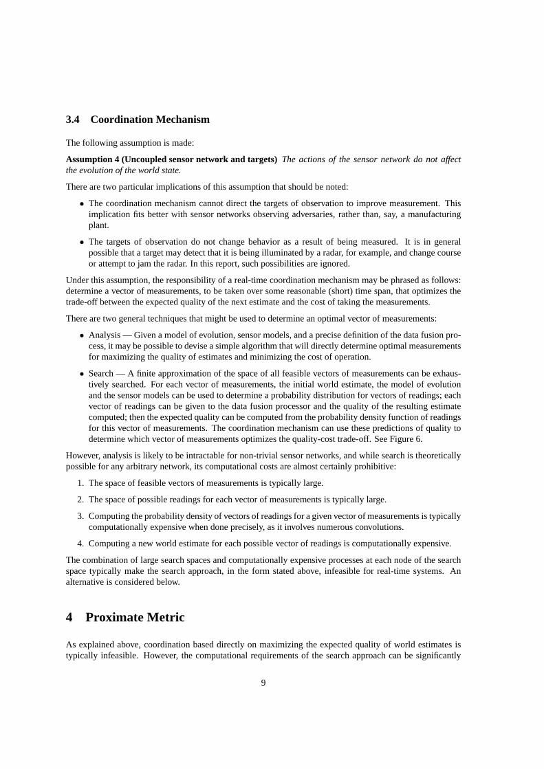
There are two particular implications of this assumption that should be noted:

• The coordination mechanism cannot direct the targets of observation to improve measurement. Thisimplication fits better with sensor networks observing adversaries, rather than, say, a manufacturingplant.

• The targets of observation do not change behavior as a result of being measured. It is in generalpossible that a target may detect that it is being illuminated by a radar, for example, and change courseor attempt to jam the radar. In this report, such possibilities are ignored.

Under this assumption, the responsibility of a real-time coordination mechanism may be phrased as follows:determine a vector of measurements, to be taken over some reasonable (short) time span, that optimizes thetrade-off between the expected quality of the next estimate and the cost of taking the measurements.

There are two general techniques that might be used to determine an optimal vector of measurements:

• Analysis — Given a model of evolution, sensor models, and a precise definition of the data fusion pro-cess, it may be possible to devise a simple algorithm that will directly determine optimal measurementsfor maximizing the quality of estimates and minimizing the cost of operation.

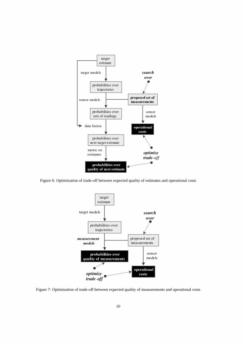
• Search — A finite approximation of the space of all feasible vectors of measurements can be exhaus-tively searched. For each vector of measurements, the initial world estimate, the model of evolutionand the sensor models can be used to determine a probability distribution for vectors of readings; eachvector of readings can be given to the data fusion processor and the quality of the resulting estimatecomputed; then the expected quality can be computed from the probability density function of readingsfor this vector of measurements. The coordination mechanism can use these predictions of quality todetermine which vector of measurements optimizes the quality-cost trade-off. See Figure 6.

However, analysis is likely to be intractable for non-trivial sensor networks, and while search is theoreticallypossible for any arbitrary network, its computational costs are almost certainly prohibitive:

1. The space of feasible vectors of measurements is typically large.

2. The space of possible readings for each vector of measurements is typically large.

3. Computing the probability density of vectors of readings for a given vector of measurements is typicallycomputationally expensive when done precisely, as it involves numerous convolutions.

4. Computing a new world estimate for each possible vector of readings is computationally expensive.

The combination of large search spaces and computationally expensive processes at each node of the searchspace typically make the search approach, in the form stated above, infeasible for real-time systems. Analternative is considered below.

4 Proximate Metric

As explained above, coordination based directly on maximizing the expected quality of world estimates istypically infeasible. However, the computational requirements of the search approach can be significantly

9

targetestimate

probabilities overtrajectories

proposed set ofmeasurements

probabilities oversets of readings

probabilities overnext target estimate

probabilities overquality of next estimate

target models

sensor models

data fusion operationalcosts

sensormodels

searchover

optimizetrade-off

metric onestimates

Figure 6: Optimization of trade-off between expected quality of estimates and operational costs

targetestimate

probabilities overtrajectories

proposed set ofmeasurements

probabilities overquality of measurements

target models

operationalcosts

sensormodels

searchover

optimizetrade -off

measurementmodels

Figure 7: Optimization of trade-off between expected quality of measurements and operational costs

10

S1

S2

S3

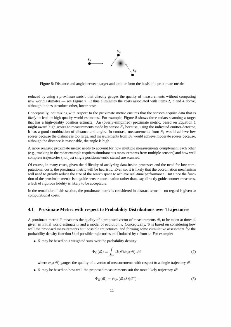
Figure 8: Distance and angle between target and emitter form the basis of a proximate metric

reduced by using aproximate metricthat directly gauges the quality of measurements without computingnew world estimates — see Figure 7. It thus eliminates the costs associated with items 2, 3 and 4 above,although it does introduce other, lower costs.

Conceptually, optimizing with respect to the proximate metric ensures that the sensors acquire data that islikely to lead to high quality world estimates. For example, Figure 8 shows three radars scanning a targetthat has a high-quality position estimate. An (overly-simplified) proximate metric, based on Equation 1might award high scores to measurements made by sensorS3 because, using the indicated emitter-detector,it has a good combination of distance and angle. In contrast, measurements fromS1 would achieve lowscores because the distance is too large, and measurements fromS2 would achieve moderate scores because,although the distance is reasonable, the angle is high.

A more realistic proximate metric needs to account for how multiple measurements complement each other(e.g., tracking in the radar example requires simultaneous measurements from multiple sensors) and how wellcomplete trajectories (not just single positions/world states) are scanned.

Of course, in many cases, given the difficulty of analyzing data fusion processes and the need for low com-putational costs, the proximate metric will be heuristic. Even so, it is likely that the coordination mechanismwill need to greatly reduce the size of the search space to achieve real-time performance. But since the func-tion of the proximate metric is to guide sensor coordination rather than, say, directly guide counter-measures,a lack of rigorous fidelity is likely to be acceptable.

In the remainder of this section, the proximate metric is considered in abstract terms — no regard is given tocomputational costs.

4.1 Proximate Metric with respect to Probability Distributions over Trajectories

A proximate metricΨ measures the quality of a proposed vector of measurements~m, to be taken at times~t,given an initial world estimateω and a model of evolutionε. Conceptually,Ψ is based on considering howwell the proposed measurements suit possible trajectories, and forming some cumulative assessment for theprobability density functionΩ of possible trajectories on~t induced byε from ω. For example:

• Ψ may be based on a weighted sum over the probability density:

ΨΩ(~m) ≡∫

~W

Ω(~w)ψ~w(~m) d~w (7)

whereψ~w(~m) gauges the quality of a vector of measurements with respect to a single trajectory~w.

• Ψ may be based on how well the proposed measurements suit the most likely trajectory~w∗:

ΨΩ(~m) ≡ ψ~w∗(~m).Ω(~w∗) . (8)

11

While this form of metric is presumably less reliable than the weighted-sum form, it may be usefulfor simple target models because its computation may be much less expensive. This form will be usedbelow in the radar example. (The quality metric includes a factor,Ω(~w∗), for how likely is the mostlikely trajectory because a trajectory that is highly likely to occur may warrant greater expenditure bythe sensor network than a trajectory that is unlikely to occur.)

Regardless of which form is chosen, the basis of the metric is the single-trajectory metricψ~w(~m) — this isconsidered in the next section.

4.2 Quality of Measurements with respect to Single Trajectory

Given a trajectory~w of world states at times~t, the qualityψ~w(~m) of a proposed vector of measurements~m (also at times~t) is a function of two terms: (i) the quality of data acquired by each measurement of itscorresponding world state, and (ii) how well the measurements complement each other.

In general, these two terms are highly application-specific — they essentially are heuristics that attempt tocharacterize the type of sensing that is likely to lead to good tracking. Here, forms appropriate for the radarexample are considered.

Section 3.2 refines term (i) into a map from individual targets in the world state to single-measurement,single-target metricsφw(m) ≡ g → φwg(m) and gives a form forφwg(m) that accounts for the possibilityof target interference.

The form of term (ii) is based on the requirement that two or three measurements from different sensors betaken approximately simultaneously, which can be accommodated using a combination of two functions:

• persistence — a function that associates a measurement with the period of time over which it couldusefully be combined with other measurements;

• adhesion — a function that, for a given timet, computes the combined quality that arises from allmeasurements whose persistence functions indicate that they can usefully contribute at timet.

These two functions and their combination are detailed below.

4.2.1 Persistence

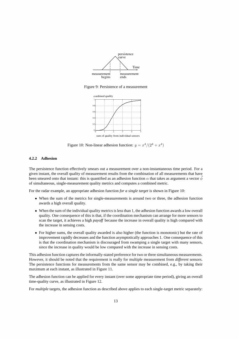
A measurement’s persistence function relates the measurement’seffectivequality at any arbitrary time to themeasurement’s peak quality (which occurs at the mid-point of the period over which the measurement wastaken). A persistence function can have arbitrary form, but typically it drops off monotonically (to zero)with distance from the measurement’s mid-point. For example, Figure 9 shows a ‘triangular’ persistencefunction.2

Specifically, for a measurement whose mid-point is at timet0 and whose quality att0 is φ0, the effectivequality at timet is given by

φt ≡ φ0π(t− t0) (9)

where the persistence functionπ has range[0, 1]. Note thatφ0 is a map from targets to single-target qualitymetrics whereasπ(t− t0) is a scalar, so computing their product involves scaling each single-target metric inφ0 uniformly, as detailed in Section 4.2.4.

2‘Persistence’ is somewhat a misnomer since there is a periodbeforethe measurement is performed for which the function is non-zero.

12

Time

measurementbegins

measurementends

persistencecurve

Figure 9: Persistence of a measurement

0

0.2

0.4

0.6

0.8

1

0 1 2 3 4 5

combined quality

sum of quality from individual sensors

Figure 10: Non-linear adhesion function:y = x4/(24 + x4)

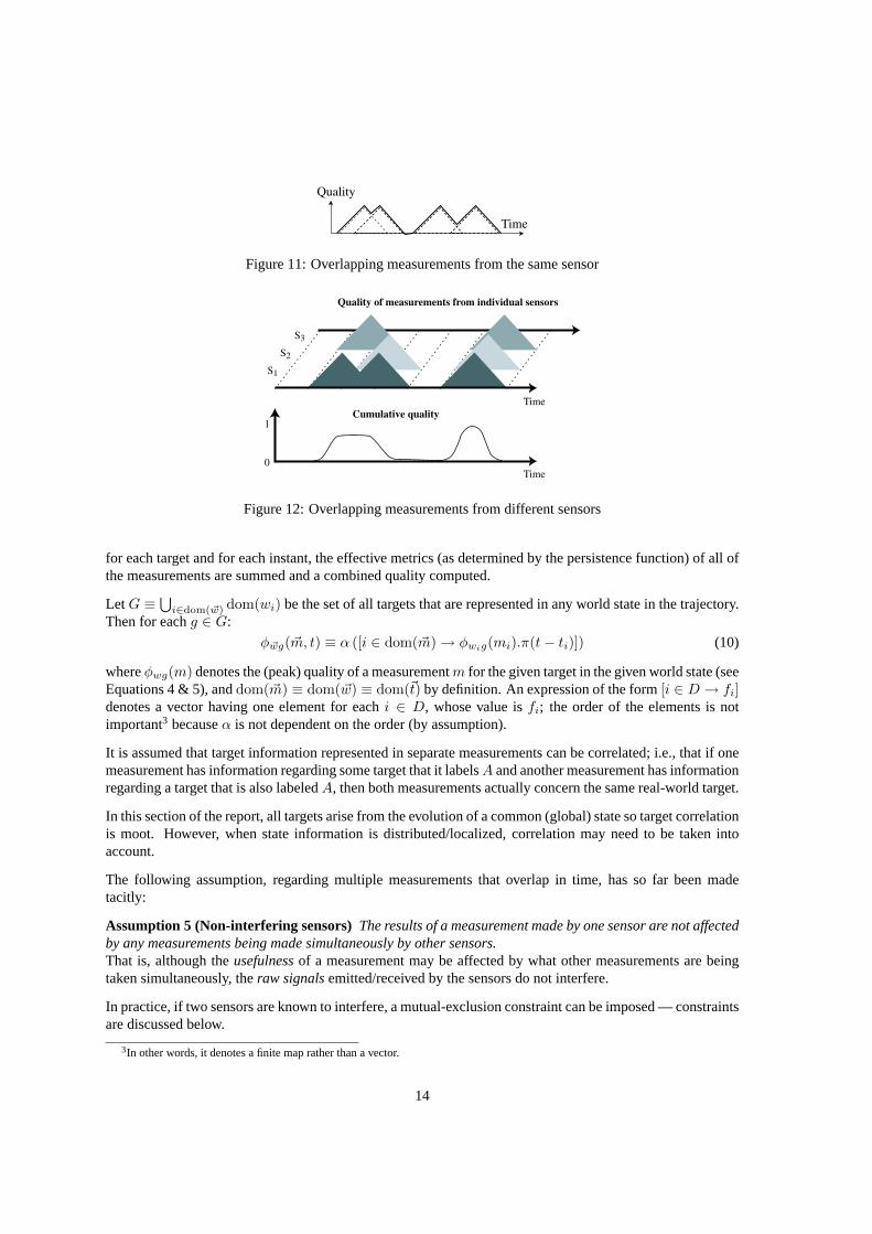
4.2.2 Adhesion

The persistence function effectively smears out a measurement over a non-instantaneous time period. For agiven instant, the overall quality of measurement results from the combination of all measurements that havebeen smeared onto that instant: this is quantified as an adhesion functionα that takes as argument a vector~φof simultaneous, single-measurement quality metrics and computes a combined metric.

For the radar example, an appropriate adhesion functionfor a single targetis shown in Figure 10:

• When the sum of the metrics for single-measurements is around two or three, the adhesion functionawards a high overall quality.

• When the sum of the individual quality metrics is less than 1, the adhesion function awards a low overallquality. One consequence of this is that, if the coordination mechanism can arrange for more sensors toscan the target, it achieves a highpayoff because the increase in overall quality is high compared withthe increase in sensing costs.

• For higher sums, the overall quality awarded is also higher (the function is monotonic) but the rate ofimprovement rapidly decreases and the function asymptotically approaches 1. One consequence of thisis that the coordination mechanism is discouraged from swamping a single target with many sensors,since the increase in quality would be low compared with the increase in sensing costs.

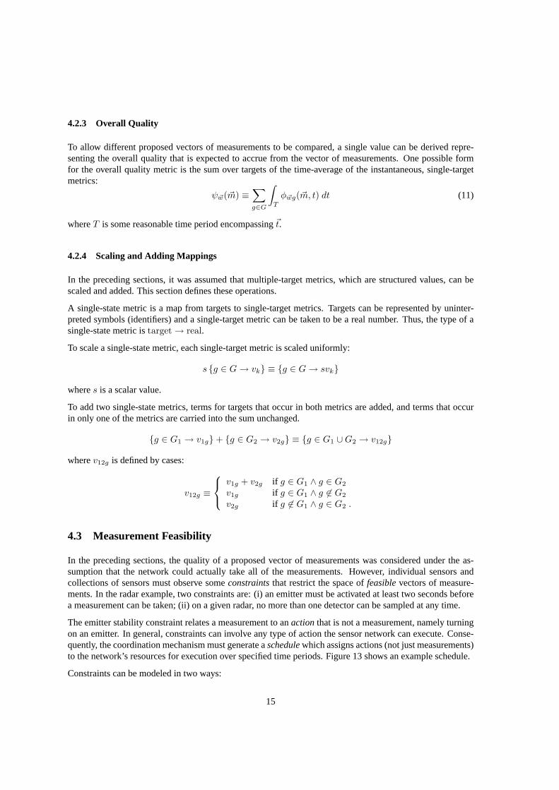
This adhesion function captures the informally-stated preference for two or three simultaneous measurements.However, it should be noted that the requirement is really for multiple measurement fromdifferentsensors.The persistence functions for measurements from the same sensor may be combined, e.g., by taking theirmaximum at each instant, as illustrated in Figure 11.

The adhesion function can be applied for every instant (over some appropriate time period), giving an overalltime-quality curve, as illustrated in Figure 12.

Formultipletargets, the adhesion function as described above applies to each single-target metric separately:

13

Quality

Time

Figure 11: Overlapping measurements from the same sensor

0

1

S1

S2

S3

Time

Time

Quality of measurements from individual sensors

Cumulative quality

Figure 12: Overlapping measurements from different sensors

for each target and for each instant, the effective metrics (as determined by the persistence function) of all ofthe measurements are summed and a combined quality computed.

LetG ≡⋃

i∈dom(~w) dom(wi) be the set of all targets that are represented in any world state in the trajectory.Then for eachg ∈ G:

φ~wg(~m, t) ≡ α ([i ∈ dom(~m) → φwig(mi).π(t− ti)]) (10)

whereφwg(m) denotes the (peak) quality of a measurementm for the given target in the given world state (seeEquations 4 & 5), anddom(~m) ≡ dom(~w) ≡ dom(~t) by definition. An expression of the form[i ∈ D → fi]denotes a vector having one element for eachi ∈ D, whose value isfi; the order of the elements is notimportant3 becauseα is not dependent on the order (by assumption).

It is assumed that target information represented in separate measurements can be correlated; i.e., that if onemeasurement has information regarding some target that it labelsA and another measurement has informationregarding a target that is also labeledA, then both measurements actually concern the same real-world target.

In this section of the report, all targets arise from the evolution of a common (global) state so target correlationis moot. However, when state information is distributed/localized, correlation may need to be taken intoaccount.

The following assumption, regarding multiple measurements that overlap in time, has so far been madetacitly:

Assumption 5 (Non-interfering sensors)The results of a measurement made by one sensor are not affectedby any measurements being made simultaneously by other sensors.That is, although theusefulnessof a measurement may be affected by what other measurements are beingtaken simultaneously, theraw signalsemitted/received by the sensors do not interfere.

In practice, if two sensors are known to interfere, a mutual-exclusion constraint can be imposed — constraintsare discussed below.

3In other words, it denotes a finite map rather than a vector.

14

4.2.3 Overall Quality

To allow different proposed vectors of measurements to be compared, a single value can be derived repre-senting the overall quality that is expected to accrue from the vector of measurements. One possible formfor the overall quality metric is the sum over targets of the time-average of the instantaneous, single-targetmetrics:

ψ~w(~m) ≡∑g∈G

∫T

φ~wg(~m, t) dt (11)

whereT is some reasonable time period encompassing~t.

4.2.4 Scaling and Adding Mappings

In the preceding sections, it was assumed that multiple-target metrics, which are structured values, can bescaled and added. This section defines these operations.

A single-state metric is a map from targets to single-target metrics. Targets can be represented by uninter-preted symbols (identifiers) and a single-target metric can be taken to be a real number. Thus, the type of asingle-state metric istarget → real.

To scale a single-state metric, each single-target metric is scaled uniformly:

s g ∈ G→ vk ≡ g ∈ G→ svk

wheres is a scalar value.

To add two single-state metrics, terms for targets that occur in both metrics are added, and terms that occurin only one of the metrics are carried into the sum unchanged.

g ∈ G1 → v1g+ g ∈ G2 → v2g ≡ g ∈ G1 ∪G2 → v12g

wherev12g is defined by cases:

v12g ≡

v1g + v2g if g ∈ G1 ∧ g ∈ G2

v1g if g ∈ G1 ∧ g 6∈ G2

v2g if g 6∈ G1 ∧ g ∈ G2 .

4.3 Measurement Feasibility

In the preceding sections, the quality of a proposed vector of measurements was considered under the as-sumption that the network could actually take all of the measurements. However, individual sensors andcollections of sensors must observe someconstraintsthat restrict the space offeasiblevectors of measure-ments. In the radar example, two constraints are: (i) an emitter must be activated at least two seconds beforea measurement can be taken; (ii) on a given radar, no more than one detector can be sampled at any time.

The emitter stability constraint relates a measurement to anactionthat is not a measurement, namely turningon an emitter. In general, constraints can involve any type of action the sensor network can execute. Conse-quently, the coordination mechanism must generate aschedulewhich assigns actions (not just measurements)to the network’s resources for execution over specified time periods. Figure 13 shows an example schedule.

Constraints can be modeled in two ways:

15

Period Resource Action0.00–0.01 radar 1 activate emitters 0 & 12.00–2.60 radar 1 sample detector 02.00–2.01 radar 2 activate emitter 22.60–3.20 radar 1 sample detector 13.20–3.21 radar 1 deactivate emitters 0 & 14.00–4.60 radar 2 sample detector 2

Figure 13: Example of a schedule

Hard constraints: a constraint is hard if its violation to any degree renders the violating measurementsuseless. For example, if a measurement is scheduled for an emitter that has been activated for 1.9seconds, then no quality accrues from the measurement.

Soft constraints: a constraint is soft if its violation results in apenaltybeing assessed against the quality ofthe vector of measurements — typically, the magnitude of the penalty increases monotonically withthe magnitude of the violation. For example, if the emitter activation constraint is modeled as a softconstraint, then a delay of 1.99 seconds before a measurement is taken would incur a small penaltycompared with that incurred for a delay of only 1.9 seconds.

Soft constraints are particularly useful when transformational search techniques (such as hill climbing orsimulated annealing) are used, in which an existing schedule is manipulated by local transform operations(such as swapping the order of two successive measurements, or transferring a measurement from one sensorto another). For such techniques, soft constraints smooth the search space and allow transformations to takeplace over schedules that would be forbidden under a hard constraint formulation, which in turn improvesconvergence properties (by reducing the number of small-scale, non-global optima).

Moreover, soft constraints tend to better capture physical systems, since there is typically some variancein physical processes: for example, it may not take an emitterexactly2.0 seconds to stabilize every time.Consequently, all constraints in this report will be assumed to be soft.

Given a schedule of actionsA and a set of soft constraintspi, the total constraint violation penalty isthe sum of the penalties for the individual constraints:P (A) ≡

∑i pi(A). (Note that each constraint can

incorporate an appropriate weighting factor.)

4.4 Overall Quality (including Operational Cost)

Given a schedule of actions, it is typically straightforward to assess the cost of executing the schedule. Forthe radar example, the main cost is the energy consumed by emitters: when an emitter is active, it consumesenergy at a constant rate, regardless of whether or not its detector is being sampled. This energy cost can becomputed from the times at which the emitters are activated and deactivated.

The details of how to assess costs do tend to be application specific, so they will not be considered furtheruntil Section 6 which gives details for the radar example. However, it is assumed that, for a scheduleA,the costsC(A) can be assessed on a scale that is commensurate with the measurement qualityMωε(A) andthe penalty metricP (A) so that an overall quality metricQ(A) can be determined. For this report, a simplelinear combination is assumed:

Qωε(A) ≡Mωε(A)− P (A)− C(A) . (12)

16

S1

S2

S3

S5

S4 S6

S7

S8

ω1 ω2

Figure 14: Fusion nodes in different parts of the network receive different measurements

An action schedule contains measurement and non-measurement actions. To determine its measurement qual-ity, the non-measurement actions are expunged to give a vector of measurements~m andΨΩ(~m) computed(see Section 4.1).

5 Coordination Mechanism

Equation 12 defines a metric functionQωε for assessing, with respect to an existing world estimate and modelof evolution, the quality of a proposed schedule of actions to be executed by a sensor network.

The responsibility of the network’s coordination mechanism may be loosely defined as determining a sched-ule that optimizesQωε. Given that a sensor network is subject to changing circumstances (such as hardwarefailing and targets not following predictions), areal-timecoordination mechanism must continually updatethe network’s schedule to maintain optimality as it learns new information about the real world.

In other words, adaptation of the sensor network to changes in the real world occurs through continualrescheduling. It would seem desirable that adaptation occur quickly, but this may not be possible in adistributed environment due to communication latency. How coordination can operate in a distributed en-vironment is considered in detail in the following sections.

5.1 Local World Estimates

The coordination mechanism is based upon knowledge of the real world, as represented by a world estimate.In order to achieve a scalable, distributed coordination mechanism, it is necessary to distribute the worldestimate as a collection of local world estimates and to maintain each local world estimate using only localmeasurements.

In this report, each sensorSj is uniquely, tightly coupled with afusion nodethat maintains a local worldestimateωj that represents information about nearby targets. Each fusion node maintains its estimate basedon readings acquired by its own sensor and on readings received from nearby sensors — each fusion nodeperiodically broadcasts its sensor’s measurements.

Since any two fusion nodes may be within communication range of different sets of sensors, the readings thatthey receive may differ, and consequently the local estimates they compute may differ. For example, Figure 14illustrates two target estimates,ω1 computed by sensorS2’s fusion node and based on measurements fromS1, S2 andS3, and estimateω2 computed by sensorS6’s fusion node and based on measurements fromS6, S7

17

CoordinationNode

ExecutionNode

TrackingNode

Sensor

localworld estimate

localschedule

instructionsreadings

measurements fromnearby sensors

schedules fromnearby sensors

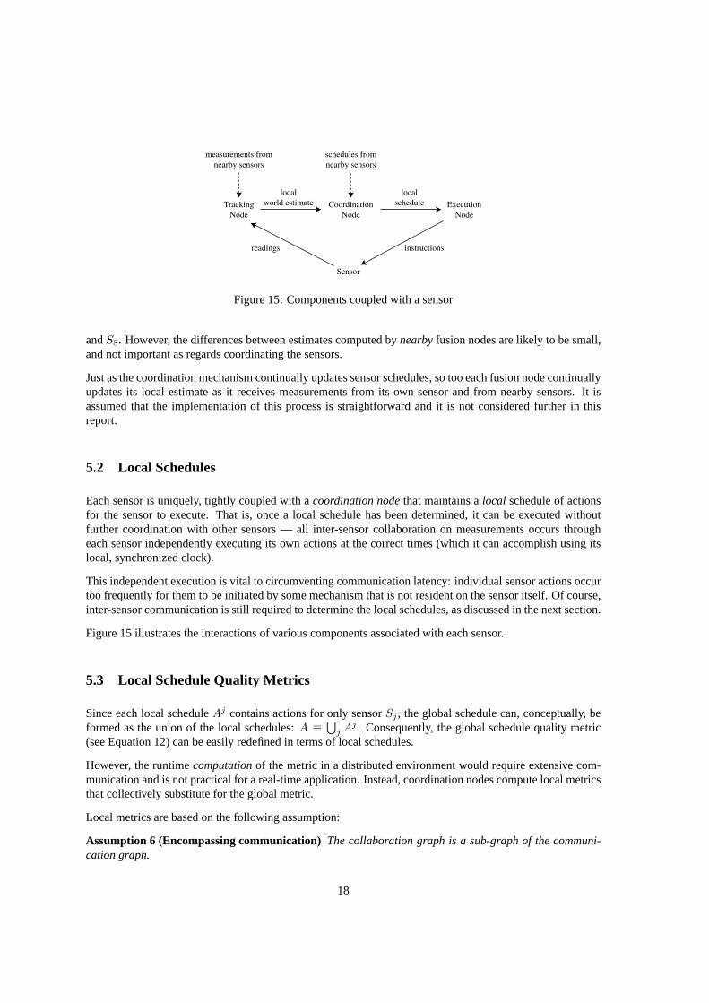
Figure 15: Components coupled with a sensor

andS8. However, the differences between estimates computed bynearbyfusion nodes are likely to be small,and not important as regards coordinating the sensors.

Just as the coordination mechanism continually updates sensor schedules, so too each fusion node continuallyupdates its local estimate as it receives measurements from its own sensor and from nearby sensors. It isassumed that the implementation of this process is straightforward and it is not considered further in thisreport.

5.2 Local Schedules

Each sensor is uniquely, tightly coupled with acoordination nodethat maintains alocal schedule of actionsfor the sensor to execute. That is, once a local schedule has been determined, it can be executed withoutfurther coordination with other sensors — all inter-sensor collaboration on measurements occurs througheach sensor independently executing its own actions at the correct times (which it can accomplish using itslocal, synchronized clock).

This independent execution is vital to circumventing communication latency: individual sensor actions occurtoo frequently for them to be initiated by some mechanism that is not resident on the sensor itself. Of course,inter-sensor communication is still required to determine the local schedules, as discussed in the next section.

Figure 15 illustrates the interactions of various components associated with each sensor.

5.3 Local Schedule Quality Metrics

Since each local scheduleAj contains actions for only sensorSj , the global schedule can, conceptually, beformed as the union of the local schedules:A ≡

⋃j A

j . Consequently, the global schedule quality metric(see Equation 12) can be easily redefined in terms of local schedules.

However, the runtimecomputationof the metric in a distributed environment would require extensive com-munication and is not practical for a real-time application. Instead, coordination nodes compute local metricsthat collectively substitute for the global metric.

Local metrics are based on the following assumption:

Assumption 6 (Encompassing communication)The collaboration graph is a sub-graph of the communi-cation graph.

18

In other words, if two sensors are capable of usefully collaborating on scanning a target, then they are capa-ble of communicating. For flat geographies and for homogeneous sensors, this assumption is satisfied if thecommunication range is twice the useful sensing range.4

Given this assumption, if every coordination node broadcasts its sensor’s schedule then each coordinationnode will know the schedules of all sensors with which direct collaboration may be useful. A local qualitymetric can be based on this knowledge, as follows.

LetHj be the set of (other) sensors with which sensorj can communicate. LetAjk(wherek ∈ Hj) bej’scopy ofk’s schedule. Then the fragment of the global schedule that is known toj is Aj ≡ Aj ∪

⋃k A

jk andj’s local quality metric isQj

ωjε ≡ Qωjε(Aj). Note that the metric is with respect to the local world estimateωj .

The global quality metric can, presumably, be expressed as a function of the local quality metrics (withappropriate account taken of the fact that each measurement may be incorporated into multiple local metrics).In general, the relationship between the global and local metrics is not simple. For example, consider aprocess in which each coordination node simultaneously changes its local schedule so as to optimize its localmetric, and assume that a stable set of local schedules is found; i.e., for everyj, Aj optimizesQj givenAjk

(k ∈ Hj). Even though every local schedule is, in a sense, locally optimal, there is no guarantee that thecombined schedule optimizes the global metric.

Nevertheless, this is essentially the process that is followed by the distributed coordination mechanism de-scribed below. The fact that global optimality is not guaranteed is viewed as a sacrifice that is required toachieve scalability and real-time responsiveness. Whether or not this sacrifice is worthwhile can only bedetermined in the context of a particular application.

5.4 Distributed Coordination Mechanism

Given the comments of the preceding sections, the objective of a distributed coordination mechanism is todetermine a set of local schedulesAj such that each local quality metricQj is optimized byAj given j’scopiesAjk (k ∈ Hj) of the local schedules of the sensors with whichj might collaborate.

To maintain scalability and real-time responsiveness, the local schedules must be determined in parallel.However, doing so raises the danger ofincoherencein which one node’s copies of its neighbors’ schedulesare being rendered obsolete even while that node is trying to optimize its own schedule with respect to them.

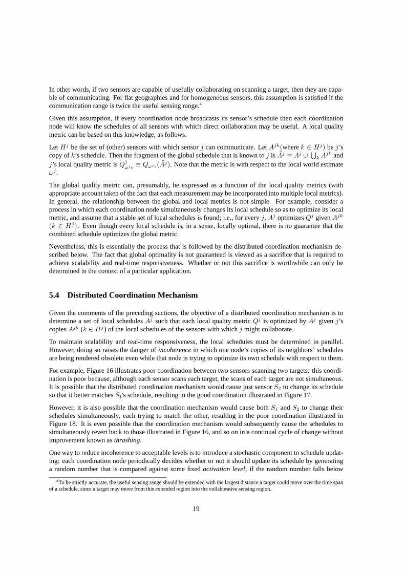
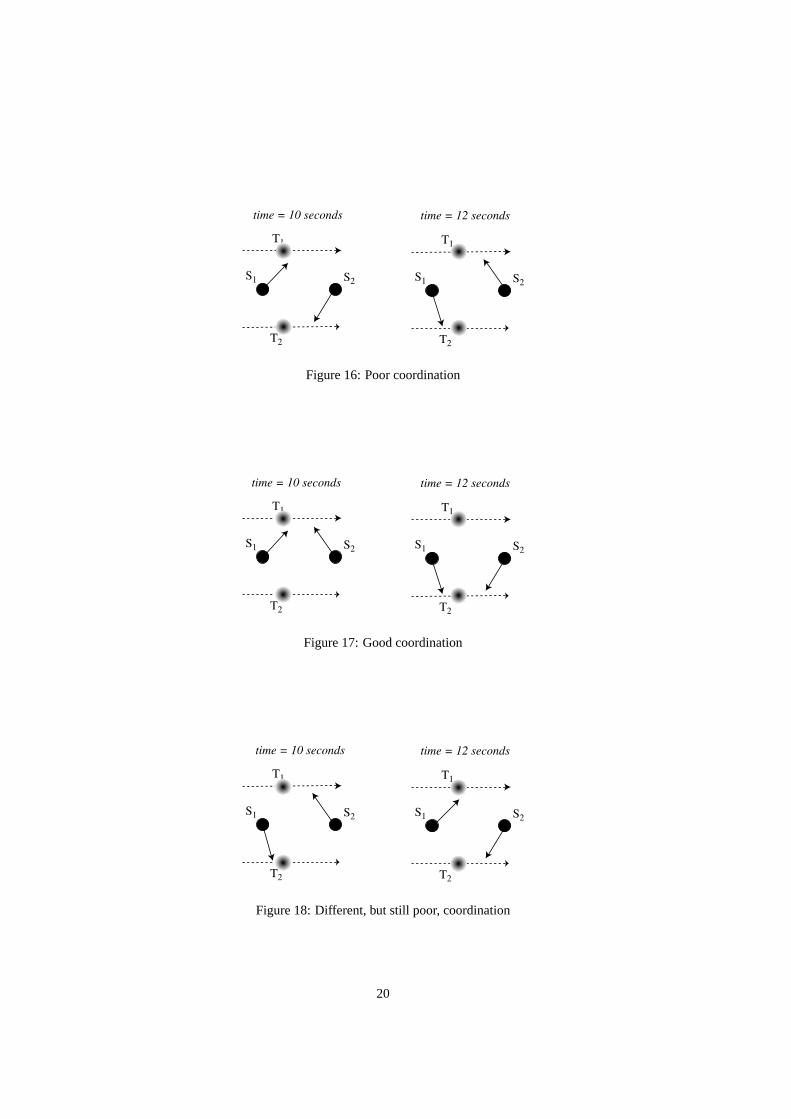
For example, Figure 16 illustrates poor coordination between two sensors scanning two targets: this coordi-nation is poor because, although each sensor scans each target, the scans of each target are not simultaneous.It is possible that the distributed coordination mechanism would cause just sensorS2 to change its scheduleso that it better matchesS1’s schedule, resulting in the good coordination illustrated in Figure 17.

However, it is also possible that the coordination mechanism would cause bothS1 andS2 to change theirschedules simultaneously, each trying to match the other, resulting in the poor coordination illustrated inFigure 18. It is even possible that the coordination mechanism would subsequently cause the schedules tosimultaneously revert back to those illustrated in Figure 16, and so on in a continual cycle of change withoutimprovement known asthrashing.

One way to reduce incoherence to acceptable levels is to introduce a stochastic component to schedule updat-ing: each coordination node periodically decides whether or not it should update its schedule by generatinga random number that is compared against some fixedactivation level; if the random number falls below

4To be strictly accurate, the useful sensing range should be extended with the largest distance a target could move over the time spanof a schedule, since a target may move from this extended region into the collaborative sensing region.

19

S1 S2

T2

T1

S1 S2

T2

T1

time = 10 seconds time = 12 seconds

Figure 16: Poor coordination

S1 S2

T2

T1

S1 S2

T2

T1

time = 10 seconds time = 12 seconds

Figure 17: Good coordination

S1 S2

T2

T1

S1 S2

T2

T1

time = 10 seconds time = 12 seconds

Figure 18: Different, but still poor, coordination

20

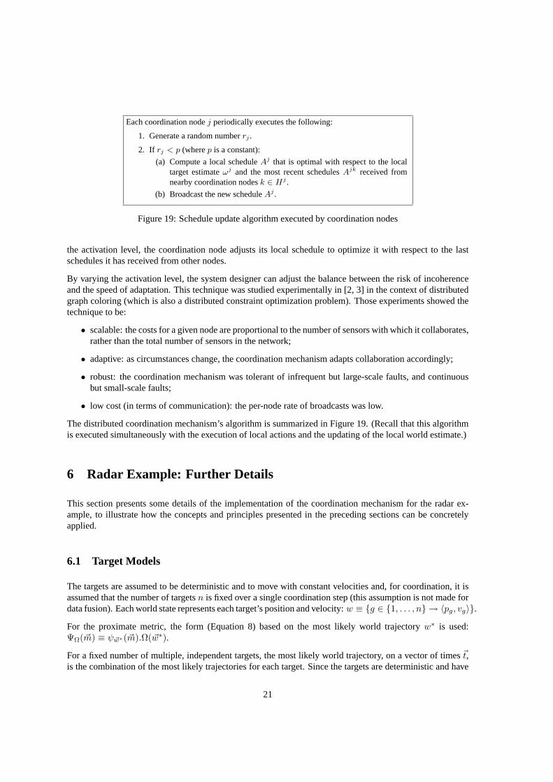
Each coordination nodej periodically executes the following:

1. Generate a random numberrj .

2. If rj < p (wherep is a constant):

(a) Compute a local scheduleAj that is optimal with respect to the localtarget estimateωj and the most recent schedulesAjk received fromnearby coordination nodesk ∈ Hj .

(b) Broadcast the new scheduleAj .

Figure 19: Schedule update algorithm executed by coordination nodes

the activation level, the coordination node adjusts its local schedule to optimize it with respect to the lastschedules it has received from other nodes.

By varying the activation level, the system designer can adjust the balance between the risk of incoherenceand the speed of adaptation. This technique was studied experimentally in [2, 3] in the context of distributedgraph coloring (which is also a distributed constraint optimization problem). Those experiments showed thetechnique to be:

• scalable: the costs for a given node are proportional to the number of sensors with which it collaborates,rather than the total number of sensors in the network;

• adaptive: as circumstances change, the coordination mechanism adapts collaboration accordingly;

• robust: the coordination mechanism was tolerant of infrequent but large-scale faults, and continuousbut small-scale faults;

• low cost (in terms of communication): the per-node rate of broadcasts was low.

The distributed coordination mechanism’s algorithm is summarized in Figure 19. (Recall that this algorithmis executed simultaneously with the execution of local actions and the updating of the local world estimate.)

6 Radar Example: Further Details

This section presents some details of the implementation of the coordination mechanism for the radar ex-ample, to illustrate how the concepts and principles presented in the preceding sections can be concretelyapplied.

6.1 Target Models

The targets are assumed to be deterministic and to move with constant velocities and, for coordination, it isassumed that the number of targetsn is fixed over a single coordination step (this assumption is not made fordata fusion). Each world state represents each target’s position and velocity:w ≡ g ∈ 1, . . . , n → 〈pg, vg〉.

For the proximate metric, the form (Equation 8) based on the most likely world trajectoryw∗ is used:ΨΩ(~m) ≡ ψ~w∗(~m).Ω(~w∗).

For a fixed number of multiple, independent targets, the most likely world trajectory, on a vector of times~t,is the combination of the most likely trajectories for each target. Since the targets are deterministic and have

21

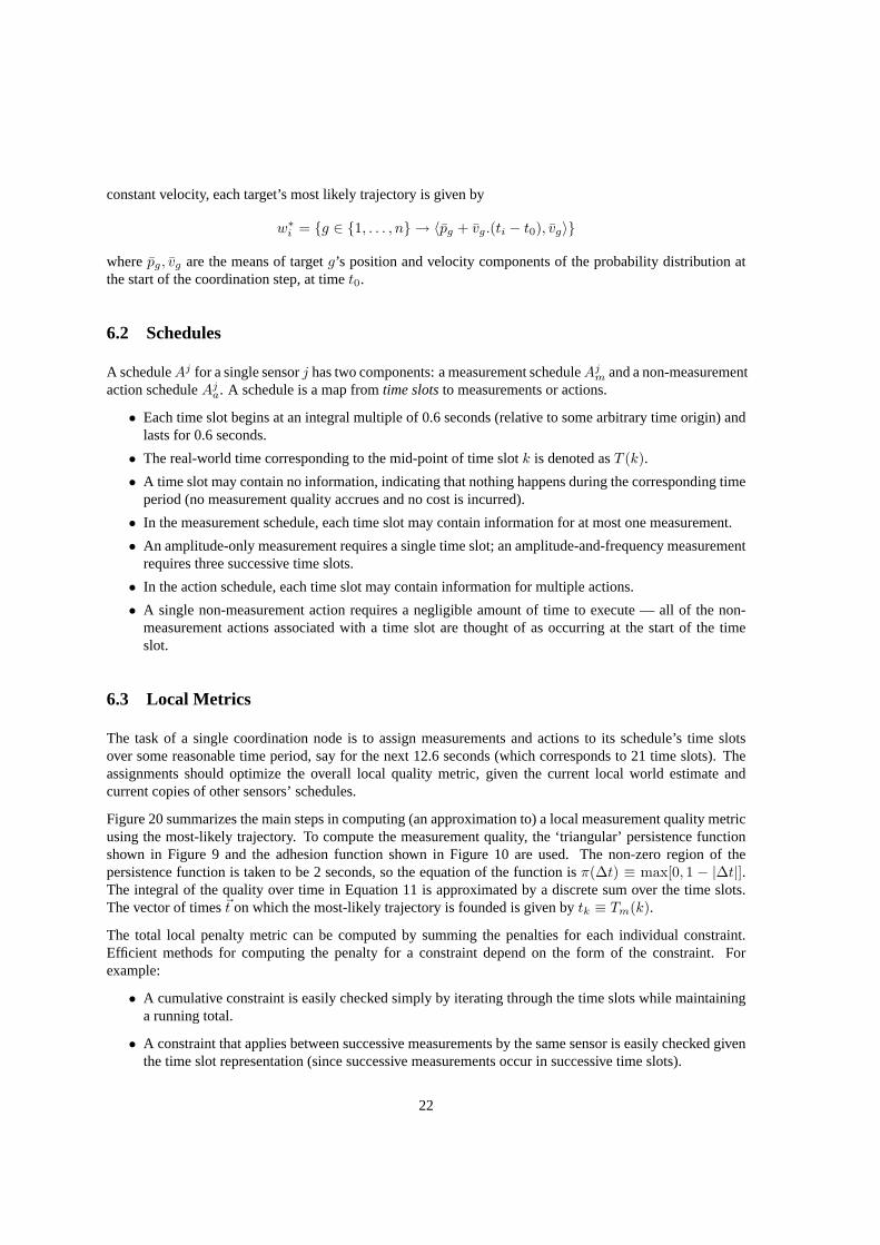
constant velocity, each target’s most likely trajectory is given by

w∗i = g ∈ 1, . . . , n → 〈pg + vg.(ti − t0), vg〉

wherepg, vg are the means of targetg’s position and velocity components of the probability distribution atthe start of the coordination step, at timet0.

6.2 Schedules

A scheduleAj for a single sensorj has two components: a measurement scheduleAjm and a non-measurement

action scheduleAja. A schedule is a map fromtime slotsto measurements or actions.

• Each time slot begins at an integral multiple of 0.6 seconds (relative to some arbitrary time origin) andlasts for 0.6 seconds.

• The real-world time corresponding to the mid-point of time slotk is denoted asT (k).

• A time slot may contain no information, indicating that nothing happens during the corresponding timeperiod (no measurement quality accrues and no cost is incurred).

• In the measurement schedule, each time slot may contain information for at most one measurement.

• An amplitude-only measurement requires a single time slot; an amplitude-and-frequency measurementrequires three successive time slots.

• In the action schedule, each time slot may contain information for multiple actions.

• A single non-measurement action requires a negligible amount of time to execute — all of the non-measurement actions associated with a time slot are thought of as occurring at the start of the timeslot.

6.3 Local Metrics

The task of a single coordination node is to assign measurements and actions to its schedule’s time slotsover some reasonable time period, say for the next 12.6 seconds (which corresponds to 21 time slots). Theassignments should optimize the overall local quality metric, given the current local world estimate andcurrent copies of other sensors’ schedules.

Figure 20 summarizes the main steps in computing (an approximation to) a local measurement quality metricusing the most-likely trajectory. To compute the measurement quality, the ‘triangular’ persistence functionshown in Figure 9 and the adhesion function shown in Figure 10 are used. The non-zero region of thepersistence function is taken to be 2 seconds, so the equation of the function isπ(∆t) ≡ max[0, 1 − |∆t|].The integral of the quality over time in Equation 11 is approximated by a discrete sum over the time slots.The vector of times~t on which the most-likely trajectory is founded is given bytk ≡ Tm(k).

The total local penalty metric can be computed by summing the penalties for each individual constraint.Efficient methods for computing the penalty for a constraint depend on the form of the constraint. Forexample:

• A cumulative constraint is easily checked simply by iterating through the time slots while maintaininga running total.

• A constraint that applies between successive measurements by the same sensor is easily checked giventhe time slot representation (since successive measurements occur in successive time slots).

22

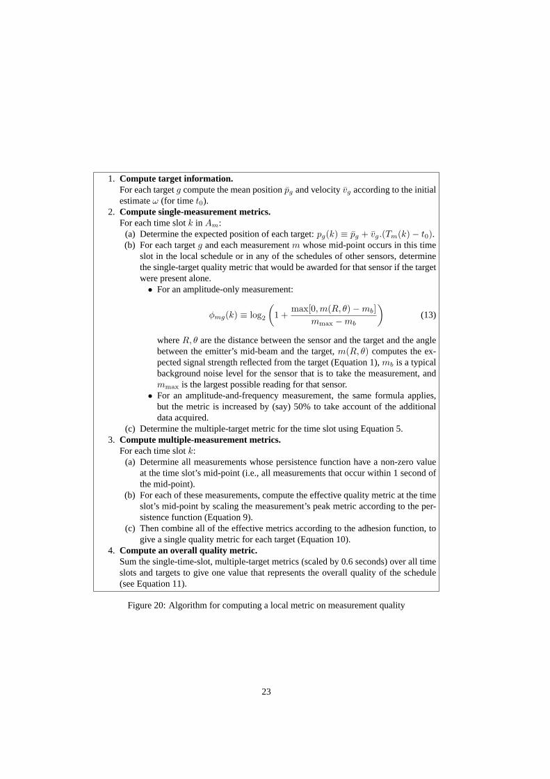
1. Compute target information.For each targetg compute the mean positionpg and velocityvg according to the initialestimateω (for time t0).

2. Compute single-measurement metrics.For each time slotk in Am:

(a) Determine the expected position of each target:pg(k) ≡ pg + vg.(Tm(k)− t0).(b) For each targetg and each measurementm whose mid-point occurs in this time

slot in the local schedule or in any of the schedules of other sensors, determinethe single-target quality metric that would be awarded for that sensor if the targetwere present alone.• For an amplitude-only measurement:

φmg(k) ≡ log2

(1 +

max[0,m(R, θ)−mb]mmax −mb

)(13)

whereR, θ are the distance between the sensor and the target and the anglebetween the emitter’s mid-beam and the target,m(R, θ) computes the ex-pected signal strength reflected from the target (Equation 1),mb is a typicalbackground noise level for the sensor that is to take the measurement, andmmax is the largest possible reading for that sensor.

• For an amplitude-and-frequency measurement, the same formula applies,but the metric is increased by (say) 50% to take account of the additionaldata acquired.

(c) Determine the multiple-target metric for the time slot using Equation 5.3. Compute multiple-measurement metrics.

For each time slotk:(a) Determine all measurements whose persistence function have a non-zero value

at the time slot’s mid-point (i.e., all measurements that occur within 1 second ofthe mid-point).

(b) For each of these measurements, compute the effective quality metric at the timeslot’s mid-point by scaling the measurement’s peak metric according to the per-sistence function (Equation 9).

(c) Then combine all of the effective metrics according to the adhesion function, togive a single quality metric for each target (Equation 10).

4. Compute an overall quality metric.Sum the single-time-slot, multiple-target metrics (scaled by 0.6 seconds) over all timeslots and targets to give one value that represents the overall quality of the schedule(see Equation 11).

Figure 20: Algorithm for computing a local metric on measurement quality

23

• A constraint between non-successive actions (such as the emitter stabilization constraint that requiresa two second delay between an emitter being activated and a measurement being taken) may be morecostly to assess. In general, each action can be interpreted as a transition function on an abstract modelof the sensor. For example, if emitter 1 is off when the action ‘activate emitter 1’ is processed, theaction causes the state of emitter 1 to switch to ‘on’ and causes a record of when 1 was last activatedto be updated.

By processing the actions in order, the effect of the schedule on the sensor can be simulated. Then theemitter stabilization constraint can be checked by determining the difference between each measure-ment’s starting time and the most recent time the appropriate emitter was activated.

• Constraints between measurements on different sensors can be checked because the other sensors’schedules are known.

The cost of executing a schedule can be determined using a simulation of the schedule’s effect on the sensor(as discussed above). For example, every time the simulation determines that an emitter is deactivated, anenergy cost can be assessed based on when the emitter was last activated.

Note: in order to produce an accurate simulation, the state of the sensor at the start of the coordination stepmust be known. This can be determined either by querying the hardware for its true state, or querying somemodel maintained by the execution node.

6.4 Search

The size of the search space for even a local schedule is large. Neglecting everything except amplitude-onlymeasurements, there are four possible choices for each time slot: a measurement one of the three detectors orno measurement. If the schedule extends over 21 time slots, the number of combinations is421 ≈ 4× 1012.This is probably too large for a generative search technique even if pruning is used.

Consequently, a transformational search algorithm is used. An initial schedule is computed by independentlychoosing for each time slot an amplitude-only measurement that maximizes the single-measurement qual-ity — collaboration, feasibility and operational costs are ignored. This schedule is then iteratively improvedusing hill-climbing on the full quality metric via transformations that include:

• Removing a measurement from a time slot, so that no measurement is performed.

• Changing the detector that is sampled in a time slot.

• Changing three successive amplitude-only measurements into an amplitude-and-frequency measure-ment.

• Inserting and removing emitter activation and deactivation actions.

(Of course, finite differencing techniques should be applied to the computation of the quality metric describedin the preceding section, so that the quality can be cheaply recomputed after transformation.)

Given that the coordination mechanism is subject to real-time constraints, it may happen that it cannot com-plete its search in time. Fortunately, a feasible schedule can be quickly extracted for execution:

• Because measurements are assigned to discrete time slots, the constraint that only one detector can besampled at any given time is automatically satisfied.

• The emitter stabilization constraint can be enforced by finding each emitter activation and removing allmeasurements involving the just-activated emitter that occur in the next three or four time slots.

24

The resulting schedule, of course, is probably not optimal (even in a local sense). However, as the executionnode begins processing the schedule, the coordination node can continue to improve it. In particular, there isstill time to change actions that are not scheduled to begin for another few seconds: consequently, the searchshould first focus on the initial section of the schedule and improve later sections only when the initial sectionhas attained sufficiently high quality.

If the transformational search algorithm ranks candidate transformations according to potential quality im-provement, then a simple way to assign more attention to the initial section of the schedule is to magnify itscontribution to the quality metric. This has the advantage of notentirelyneglecting later parts of the schedule.

Of course, it may happen that even with its ongoing, anytime search approach, the coordination node issimply incapable of producing schedules of sufficiently high quality in the time and with the computationalpower available. To determine if this is so, a detailed analysis of the probability distribution of schedulesand consequent computational costs associated with the search and metric algorithms may be performed.Alternatively, the approach can be validated experimentally.

7 Conclusion

This report details a scalable, distributed, real-time coordination mechanism for local sensors interactingover a local, high-latency communication fabric. The general problem is defined as achieving high-qualityestimates of the real world while minimizing operational costs.

Because the general problem is typically too computationally expensive for real-time systems, a simplerproblem is introduced — achieving high-quality sensing while minimizing operational costs. It is hoped thatsolving the simpler problem will lead to world estimates of acceptable quality.

An approximate form of the problem of achieving high-quality sensing is defined for distributed systems inwhich communication latency requires all interaction to be local. A practical implementation is consideredfor a network of simple radar sensors.

An experimental assessment of the coordination mechanism for the radar network should be available in asubsequent report.

It may be speculated that the heuristic components of the definition of sensing quality could be made rig-orous in information-theoretic terms by considering entropic metrics on world estimates and the amount ofinformation conveyed by measurements, under the assumption that high-quality estimates are those that havehigh information content. This would be an interesting topic for further research.

References

[1] The ANTs Challenge Problem,http://ants.kestrel.edu/challenge-problem/index.html

[2] Soft, Real-Time, Distributed Graph Coloring using Decentralized, Synchronous, Stochastic, Iterative-Repair, Anytime Algorithms. A Framework, Stephen Fitzpatrick & Lambert Meertens, Technical ReportKES.U.01.05, Kestrel Institute, May 2001

[3] An Experimental Assessment of a Stochastic, Anytime, Decentralized, Soft Colourer for Sparse GraphsTo appear: Proceedings of SAGA 2001,1st Symposium on Stochastic Algorithms, Foundations and Ap-plications, Berlin, 13-14 December 2001, Springer-Verlag.

25