Embed Size (px)
Citation preview
Pegasus Lectures, Inc.
Volume II
Companion Presentation
Frank R. MielePegasus Lectures, Inc.
Ultrasound Physics & Instrumentation4th Edition
Pegasus Lectures, Inc.
License Agreement
This presentation is the sole property of Pegasus Lectures, Inc.
No part of this presentation may be copied or used for any purpose other than as part of the partnership program as described in the
license agreement. Materials within this presentation may not be used in any part or form outside of the partnership program. Failure to follow
the license agreement is a violation of Federal Copyright Law.
All Copyright Laws Apply.
Pegasus Lectures, Inc.
Volume II Outline
Chapter 7: Doppler
Chapter 8: Artifacts
Chapter 9: Bioeffects
Chapter 10: Contrast and Harmonics
Chapter 11: Quality Assurance
Chapter 12: Fluid Dynamics
Level 2
Chapter 13: Hemodynamics
Pegasus Lectures, Inc.
Energy
Potential Energy: Energy which is stored -- the ability to do work
Kinetic Energy: Energy which is related to motion – proportional to the velocity squared
Conservation of Energy: Energy is always conserved – energy is never lost, only converted between forms
Pegasus Lectures, Inc.
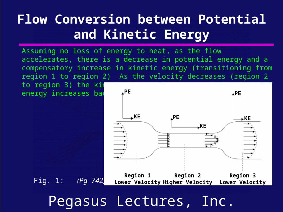
Assuming no loss of energy to heat, as the flow accelerates, there is a decrease in potential energy and a compensatory increase in kinetic energy (transitioning from region 1 to region 2) As the velocity decreases (region 2 to region 3) the kinetic energy decreases and the potential energy increases back to the same level as in region 1.
Flow Conversion between Potential and Kinetic Energy
Fig. 1: (Pg 742)
PE
KE PE
KE
PE
KE
Region 1Lower Velocity
Region 2Higher Velocity
Region 3Lower Velocity
Pegasus Lectures, Inc.
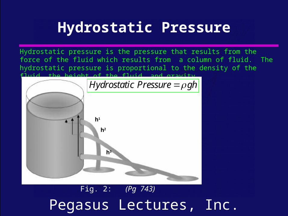
Hydrostatic pressure is the pressure that results from the force of the fluid which results from a column of fluid. The hydrostatic pressure is proportional to the density of the fluid, the height of the fluid, and gravity.
Hydrostatic Pressure
Fig. 2: (Pg 743)
h1
h2
h3
Hydrostatic Pressure gh
Pegasus Lectures, Inc.
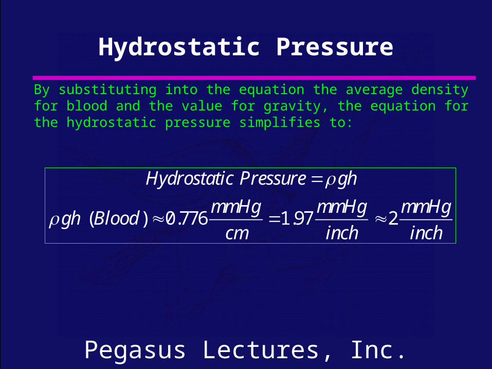
By substituting into the equation the average density for blood and the value for gravity, the equation for the hydrostatic pressure simplifies to:
Hydrostatic Pressure
( ) 0.776 1.97 2
Hydrostatic Pressure gh
mmHg mmHg mmHggh Blood
cm inch inch
Pegasus Lectures, Inc.
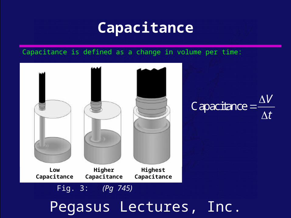
Capacitance is defined as a change in volume per time:
Capacitance
Fig. 3: (Pg 745)
LowCapacitance
HigherCapacitance
HighestCapacitance
CapacitanceV
t
Pegasus Lectures, Inc.
The principal relationships that constitute the resistance equation are developed throughout the next group of slides. Instead of just writing the equation outright, we will consider different physical situations to gain an intuitive understanding of these relationships.
Developing the Resistance Equation
Pegasus Lectures, Inc.
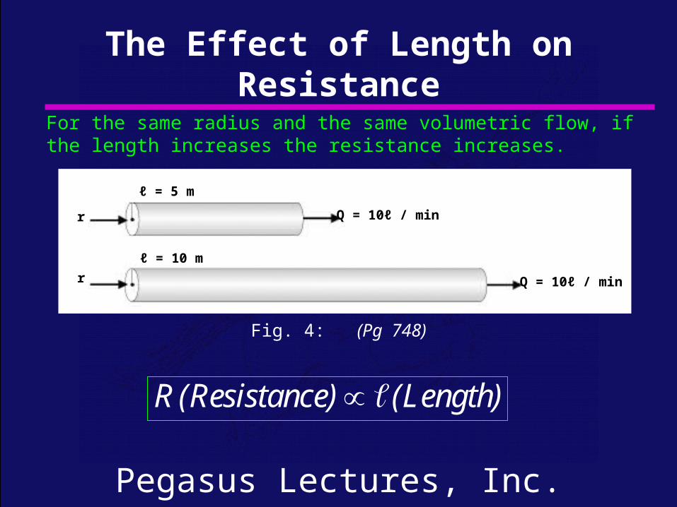
For the same radius and the same volumetric flow, if the length increases the resistance increases.
The Effect of Length on Resistance
Fig. 4: (Pg 748)
ℓ = 5 m
ℓ = 10 m
Q = 10ℓ / min
Q = 10ℓ / min
r
r
R (Resistance) (Length)
Pegasus Lectures, Inc.
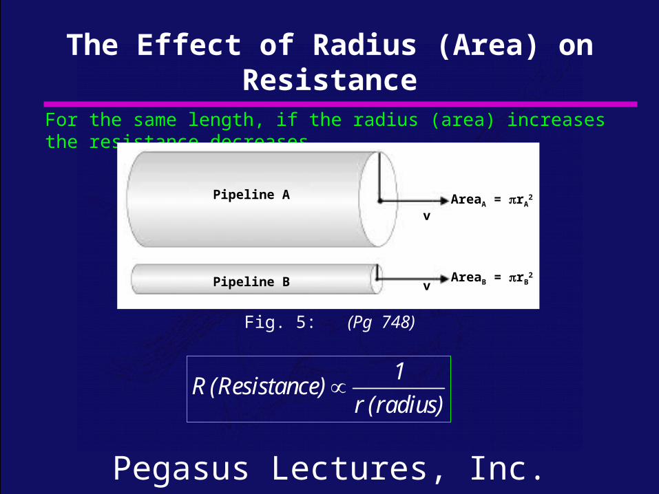
The Effect of Radius (Area) on Resistance
For the same length, if the radius (area) increases the resistance decreases.
Fig. 5: (Pg 748)
Pipeline A
Pipeline B
v
v
AreaA = rA2
AreaB = rB2
1R (Resistance)
r (radius)
Pegasus Lectures, Inc.
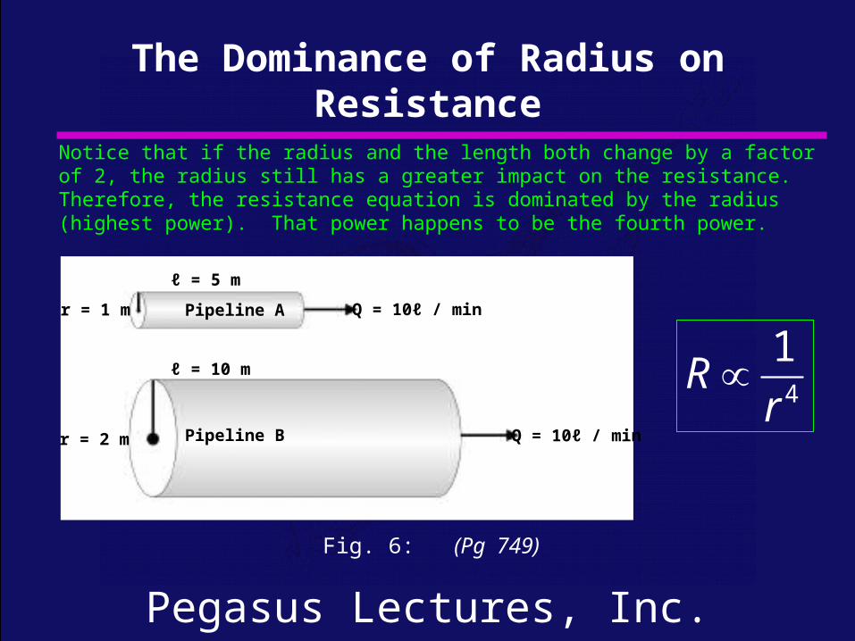
The Dominance of Radius on Resistance
Notice that if the radius and the length both change by a factor of 2, the radius still has a greater impact on the resistance. Therefore, the resistance equation is dominated by the radius (highest power). That power happens to be the fourth power.
Pipeline A
Pipeline B
Q = 10ℓ / min
Q = 10ℓ / min
r = 1 m
r = 2 m
ℓ = 5 m
ℓ = 10 m
Fig. 6: (Pg 749)
4
1R
r
Pegasus Lectures, Inc.
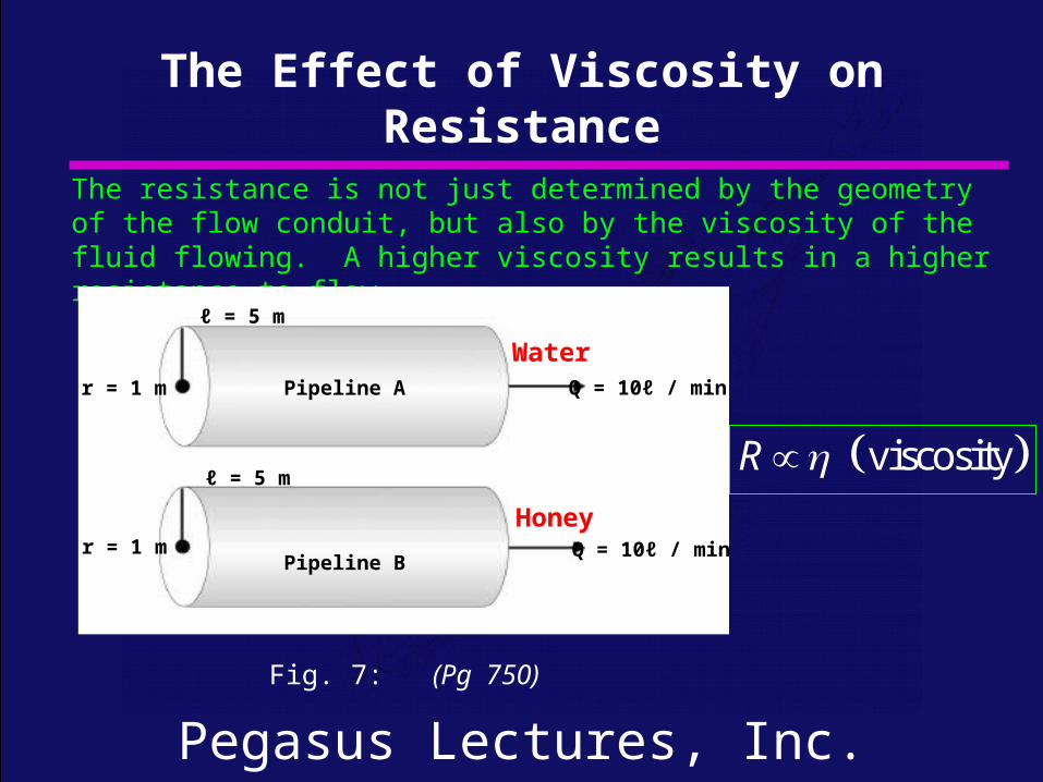
The Effect of Viscosity on Resistance
The resistance is not just determined by the geometry of the flow conduit, but also by the viscosity of the fluid flowing. A higher viscosity results in a higher resistance to flow.
Fig. 7: (Pg 750)
Pipeline A
Pipeline B
Q = 10ℓ / min
Q = 10ℓ / min
r = 1 m
r = 1 m
ℓ = 5 m
ℓ = 5 m
Water
Honey
viscosityR
Pegasus Lectures, Inc.
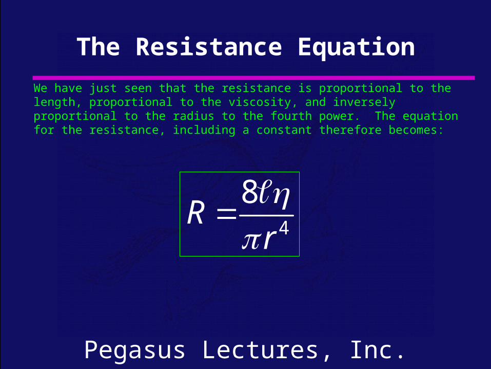
We have just seen that the resistance is proportional to the length, proportional to the viscosity, and inversely proportional to the radius to the fourth power. The equation for the resistance, including a constant therefore becomes:
The Resistance Equation
4
8R
r
Pegasus Lectures, Inc.
The principal relationships that constitute the continuity equation are developed throughout the next group of slides. As with the resistance equation, instead of just writing the equation outright, we will consider different physical situations to gain an intuitive understanding of these relationships.
Developing the Continuity (Volumetric Flow) Equation
Pegasus Lectures, Inc.
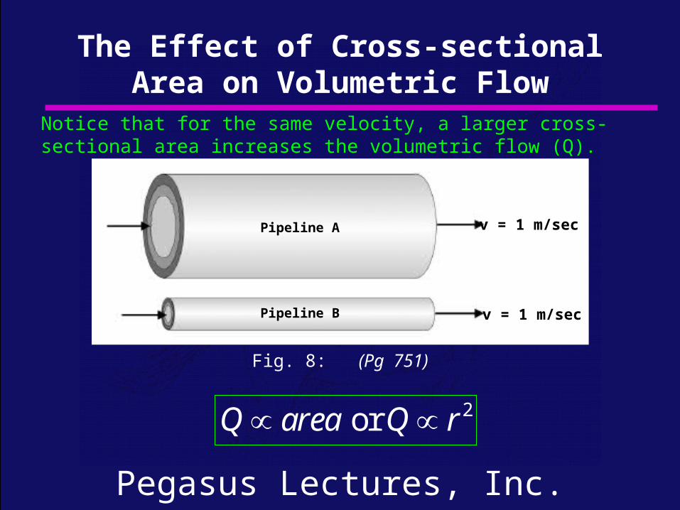
The Effect of Cross-sectional Area on Volumetric Flow
Notice that for the same velocity, a larger cross-sectional area increases the volumetric flow (Q).
Fig. 8: (Pg 751)
Pipeline A
Pipeline B
v = 1 m/sec
v = 1 m/sec
2 or Q area Q r
Pegasus Lectures, Inc.
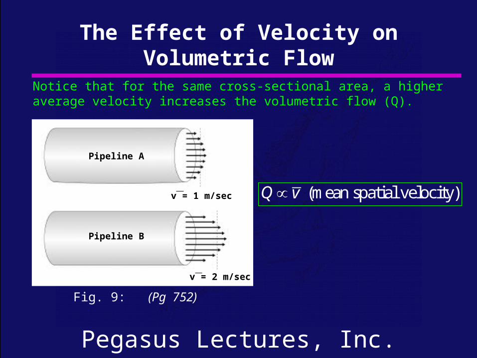
The Effect of Velocity on Volumetric Flow
Notice that for the same cross-sectional area, a higher average velocity increases the volumetric flow (Q).
Fig. 9: (Pg 752)
Pipeline A
Pipeline B
v = 1 m/sec
v = 2 m/sec
(mean spatial velocity)Q v
Pegasus Lectures, Inc.
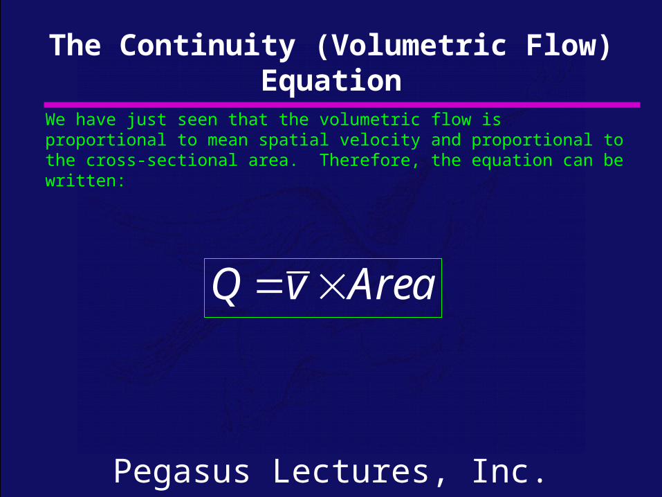
We have just seen that the volumetric flow is proportional to mean spatial velocity and proportional to the cross-sectional area. Therefore, the equation can be written:
The Continuity (Volumetric Flow) Equation
Q v Area
Pegasus Lectures, Inc.
The principal relationships that constitute the equation for the simplified law of hemodynamics are developed throughout the next group of slides. As with the resistance equation and the flow equation (continuity equation), instead of just writing the equation outright, we will consider different physical situations to gain an intuitive understanding of these relationships.
Developing the Simplified Law of Hemodynamics
Pegasus Lectures, Inc.
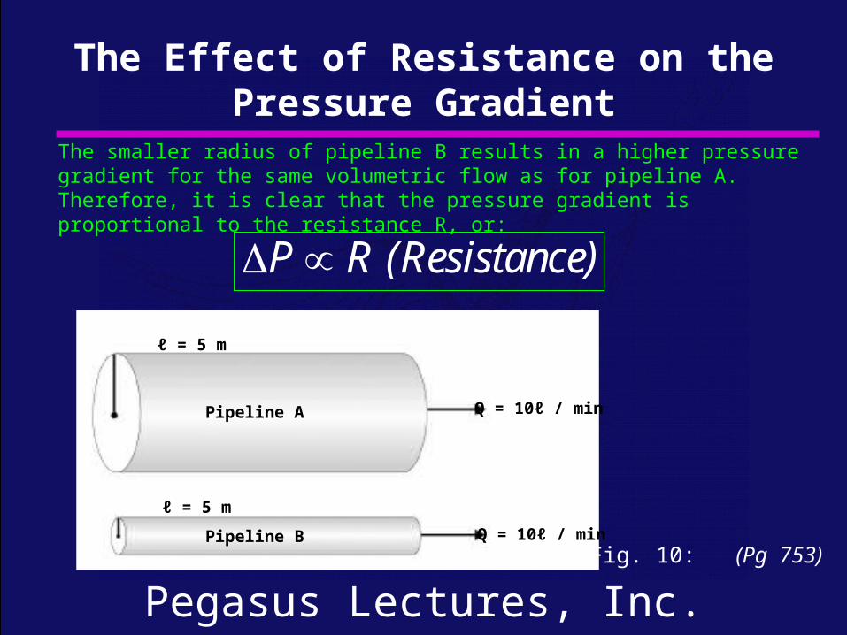
The Effect of Resistance on the Pressure Gradient
The smaller radius of pipeline B results in a higher pressure gradient for the same volumetric flow as for pipeline A. Therefore, it is clear that the pressure gradient is proportional to the resistance R, or:
Fig. 10: (Pg 753)
Pipeline A
Pipeline B
Q = 10ℓ / min
Q = 10ℓ / min
ℓ = 5 m
ℓ = 5 m
P R (Resistance)
Pegasus Lectures, Inc.
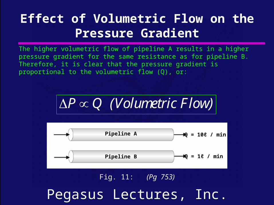
Effect of Volumetric Flow on the Pressure Gradient
Fig. 11: (Pg 753)
Pipeline A
Pipeline B
Q = 10ℓ / min
Q = 1ℓ / min
The higher volumetric flow of pipeline A results in a higher pressure gradient for the same resistance as for pipeline B. Therefore, it is clear that the pressure gradient is proportional to the volumetric flow (Q), or:
P Q (Volumetric Flow)
Pegasus Lectures, Inc.
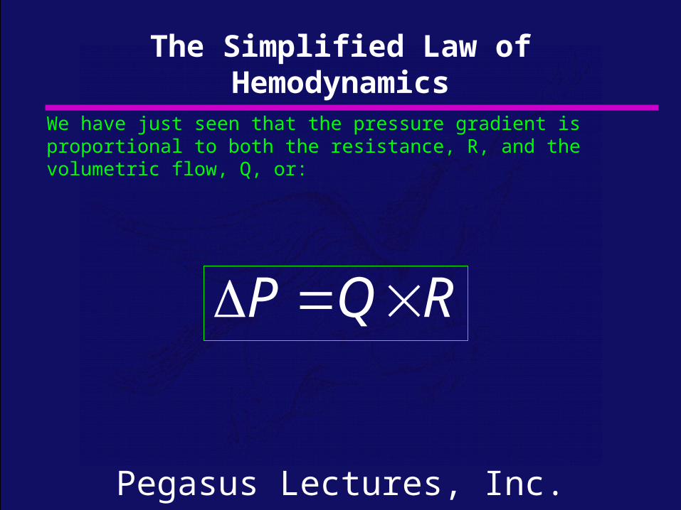
We have just seen that the pressure gradient is proportional to both the resistance, R, and the volumetric flow, Q, or:
The Simplified Law of Hemodynamics
P Q R
Pegasus Lectures, Inc.
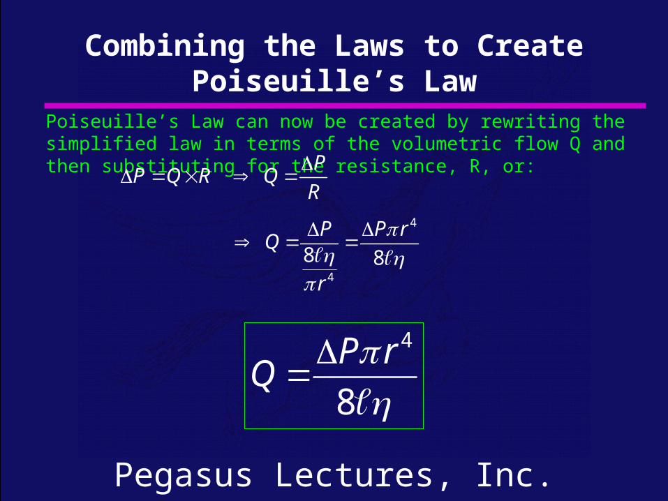
Combining the Laws to Create Poiseuille’s Law
Poiseuille’s Law can now be created by rewriting the simplified law in terms of the volumetric flow Q and then substituting for the resistance, R, or:
4
4
8 8
PP Q R Q
R
P P rQ
r
4
8
P rQ
Pegasus Lectures, Inc.
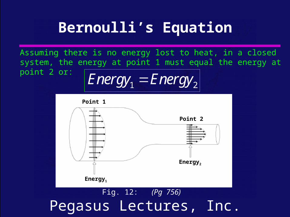
Bernoulli’s Equation
Point 2
Point 1
Energy1
Energy2
Assuming there is no energy lost to heat, in a closed system, the energy at point 1 must equal the energy at point 2 or:
1 2Energy Energy
Fig. 12: (Pg 756)
Pegasus Lectures, Inc.
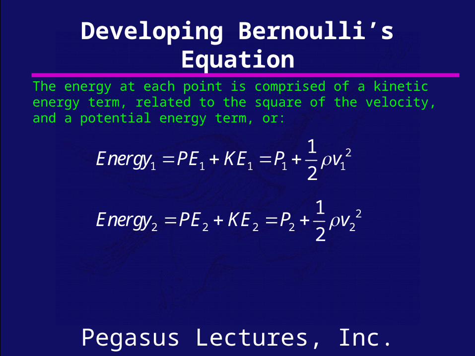
Developing Bernoulli’s Equation
The energy at each point is comprised of a kinetic energy term, related to the square of the velocity, and a potential energy term, or:
21 1 1 1 1
22 2 2 2 2
1
2
1
2
Energy PE KE P v
Energy PE KE P v
Pegasus Lectures, Inc.
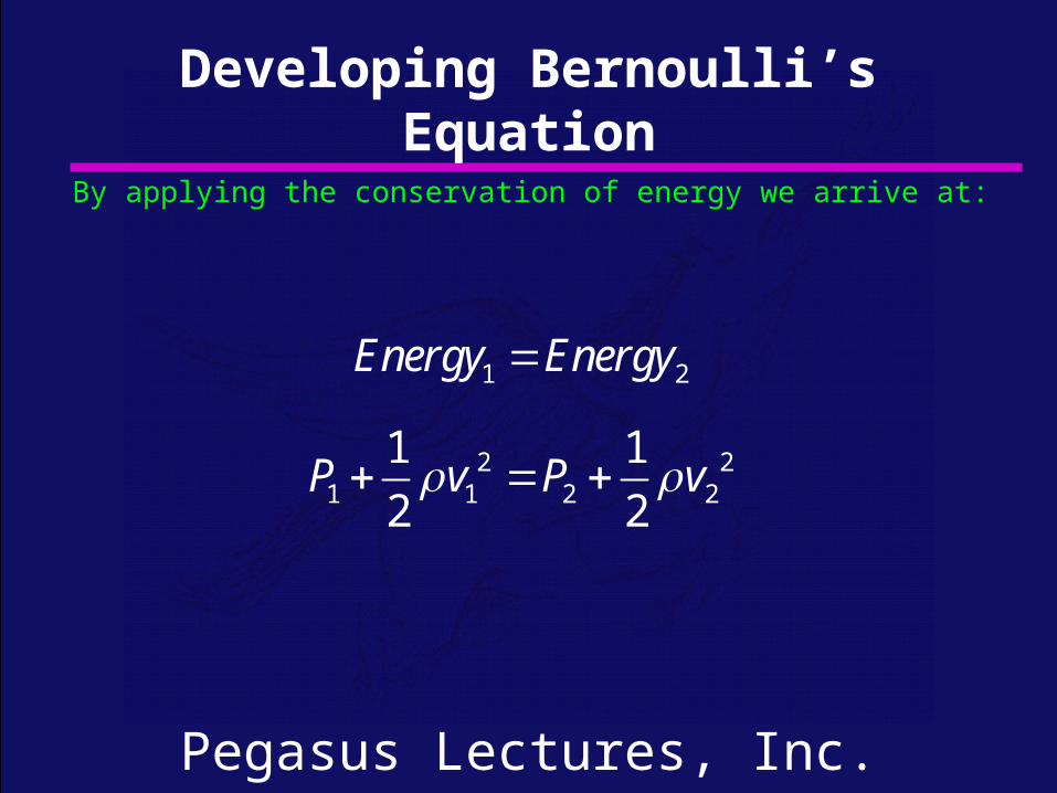
Developing Bernoulli’s Equation
By applying the conservation of energy we arrive at:
1 2
2 21 1 2 2
1 1
2 2
Energy Energy
P v P v
Pegasus Lectures, Inc.
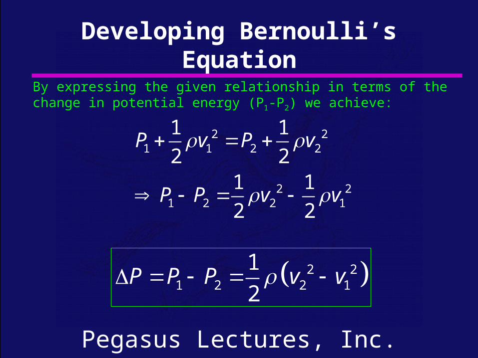
Developing Bernoulli’s Equation
By expressing the given relationship in terms of the change in potential energy (P1-P2) we achieve:
2 21 1 2 2
2 21 2 2 1
1 1
2 21 1
2 2
P v P v
P P v v
2 21 2 2 1
1
2P P P v v
Pegasus Lectures, Inc.
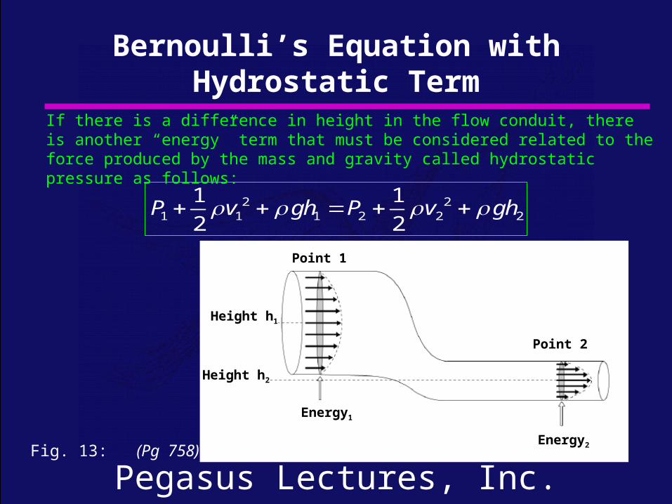
Bernoulli’s Equation with Hydrostatic Term
Height h1
Height h2
Energy1
Energy2
Point 2
Point 1
If there is a difference in height in the flow conduit, there is another “energy” term that must be considered related to the force produced by the mass and gravity called hydrostatic pressure as follows:
2 21 1 1 2 2 2
1 1
2 2P v gh P v gh
Fig. 13: (Pg 758)
Pegasus Lectures, Inc.
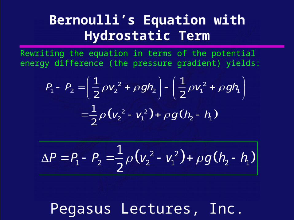
Bernoulli’s Equation with Hydrostatic Term
Rewriting the equation in terms of the potential energy difference (the pressure gradient) yields:
2 21 2 2 2 1 1
2 22 1 2 1
1 1
2 2
1
2
P P v gh v gh
v v g h h
2 21 2 2 1 2 1
1
2P P P v v g h h
Pegasus Lectures, Inc.
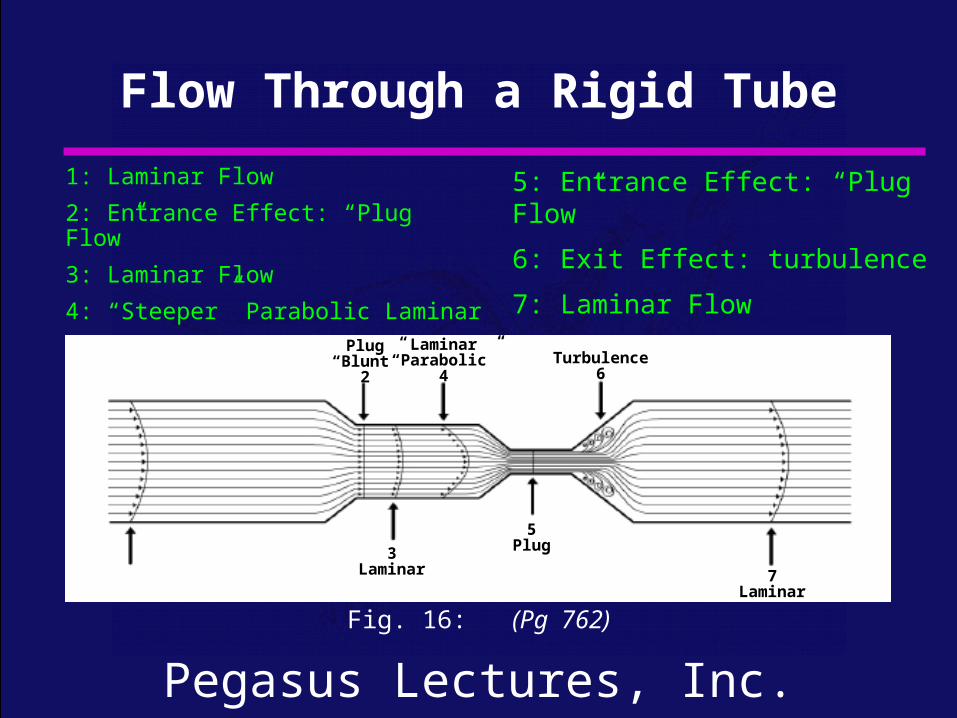
1: Laminar Flow
2: Entrance Effect: “Plug Flow”
3: Laminar Flow
4: “Steeper” Parabolic Laminar
Flow Through a Rigid Tube
Fig. 16: (Pg 762)
1Laminar
Plug“Blunt”
2
Laminar“Parabolic”
4Turbulence
6
3Laminar 7
Laminar
5Plug
5: Entrance Effect: “Plug Flow”
6: Exit Effect: turbulence
7: Laminar Flow
Pegasus Lectures, Inc.
Flow Examples
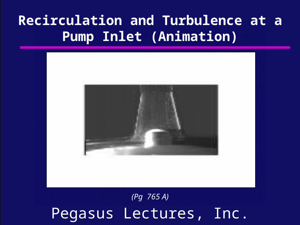
The following slides are taken from the animation CD demonstrating various flow conditions and states (videos courtesy of Flometrics of Solana Beach California). It is very beneficial to review the animation CD for more in depth descriptions.
Pegasus Lectures, Inc.
Recirculation and Turbulence at a Pump Inlet (Animation)
(Pg 765 A)
Pegasus Lectures, Inc.
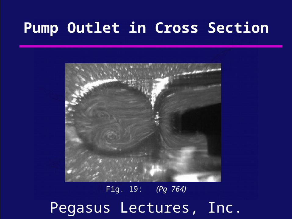
Pump Outlet in Cross Section
Fig. 19: (Pg 764)
Pegasus Lectures, Inc.
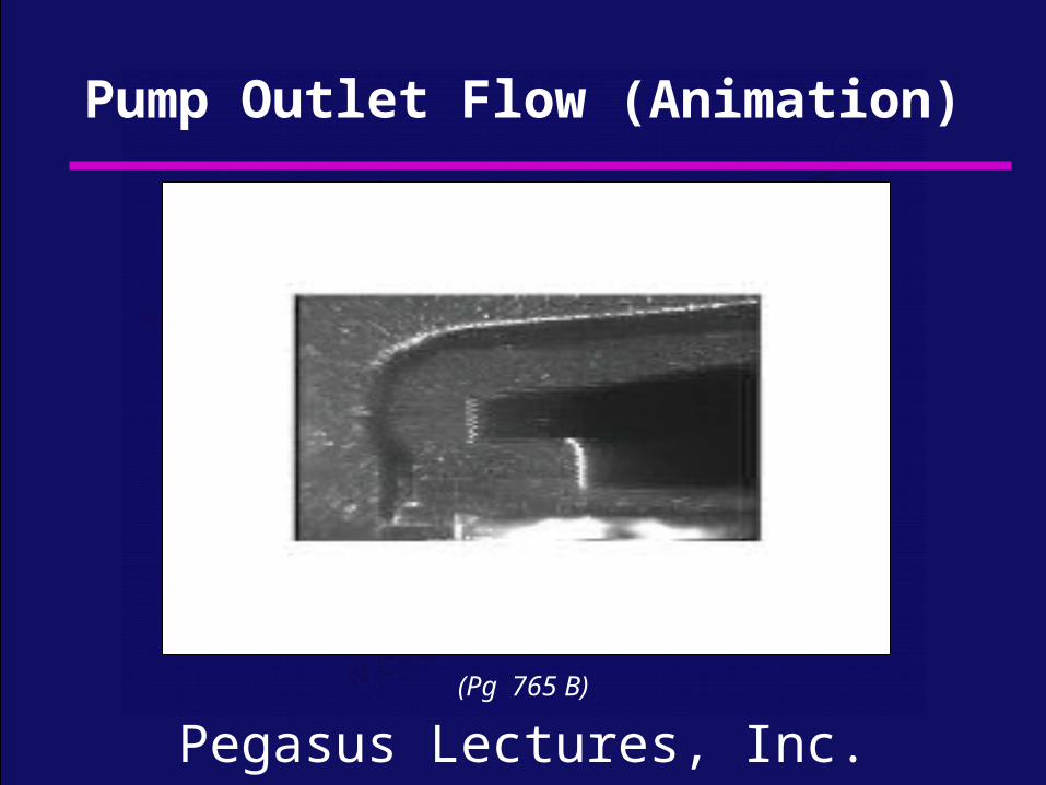
Pump Outlet Flow (Animation)
(Pg 765 B)
Pegasus Lectures, Inc.
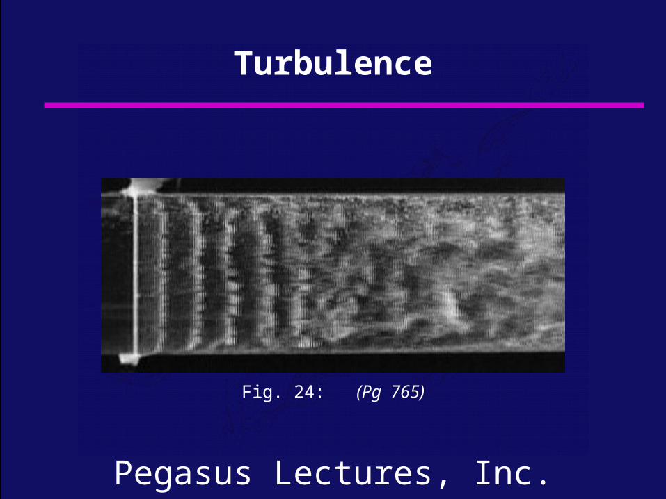
Turbulence
Fig. 24: (Pg 765)
Pegasus Lectures, Inc.
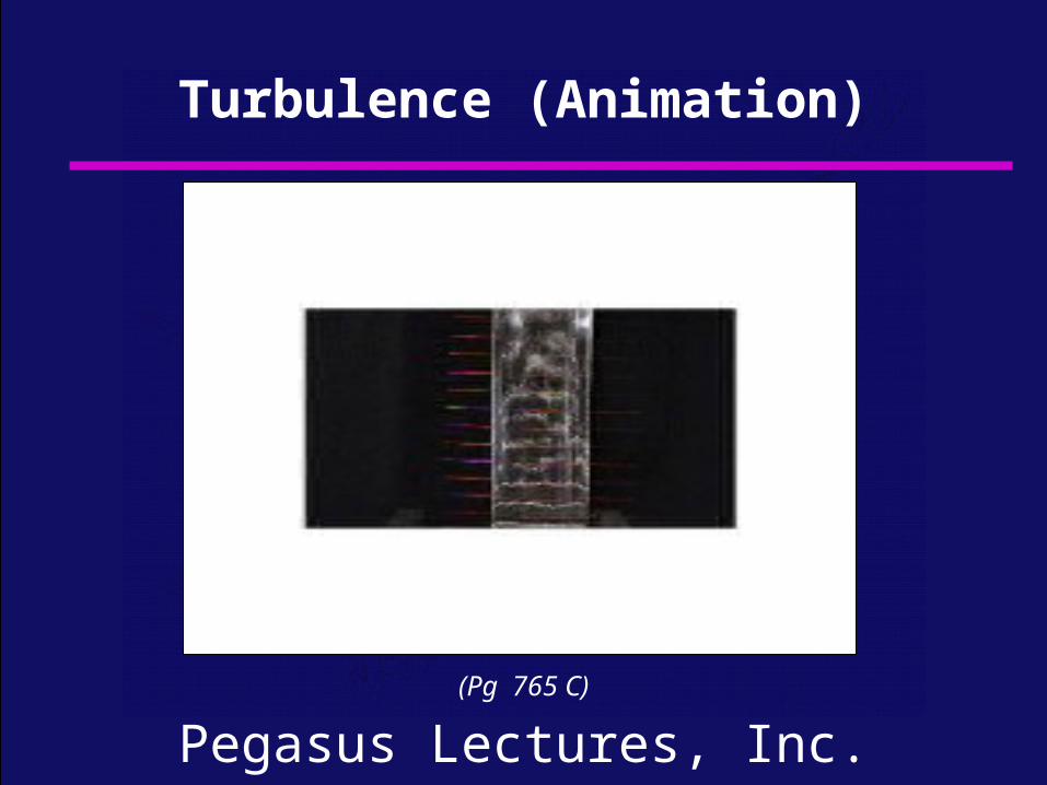
Turbulence (Animation)
(Pg 765 C)
Pegasus Lectures, Inc.
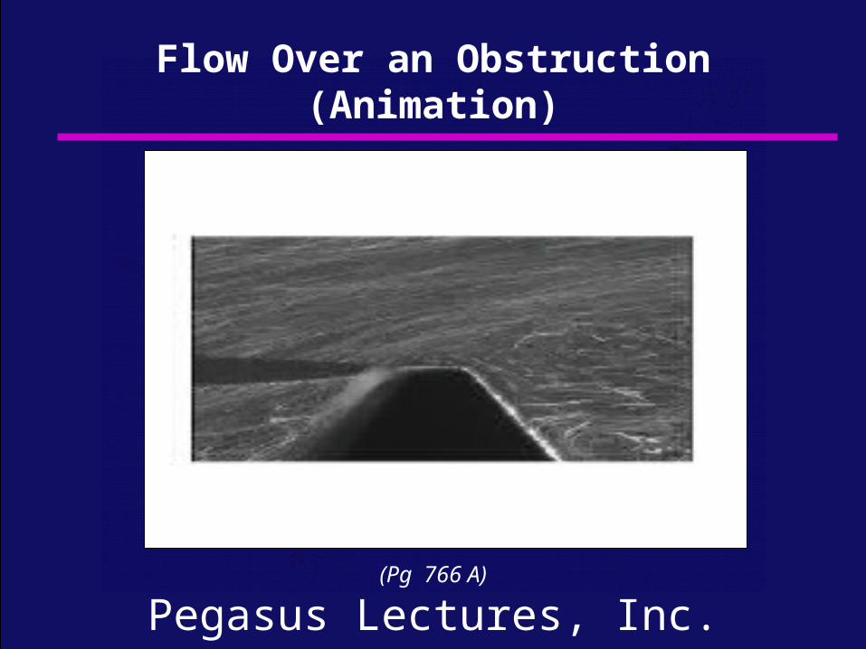
Flow Over an Obstruction (Animation)
(Pg 766 A)
Pegasus Lectures, Inc.
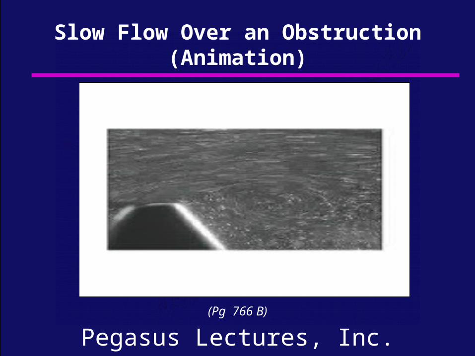
Slow Flow Over an Obstruction (Animation)
(Pg 766 B)
Pegasus Lectures, Inc.
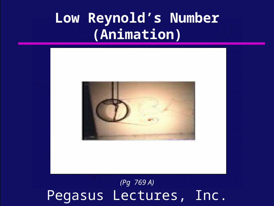
Low Reynold’s Number (Animation)
(Pg 769 A)
Pegasus Lectures, Inc.
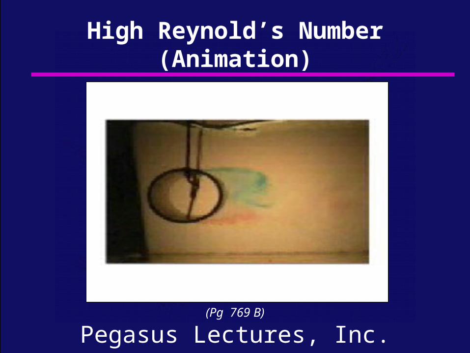
High Reynold’s Number (Animation)
(Pg 769 B)
Pegasus Lectures, Inc.
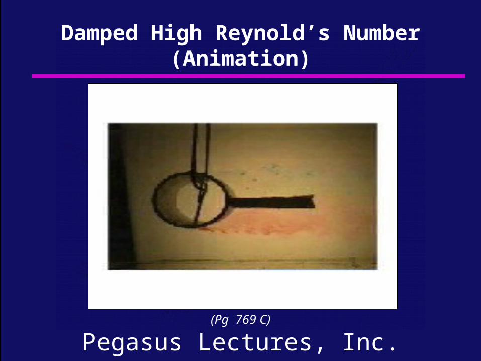
Damped High Reynold’s Number (Animation)
(Pg 769 C)
Pegasus Lectures, Inc.
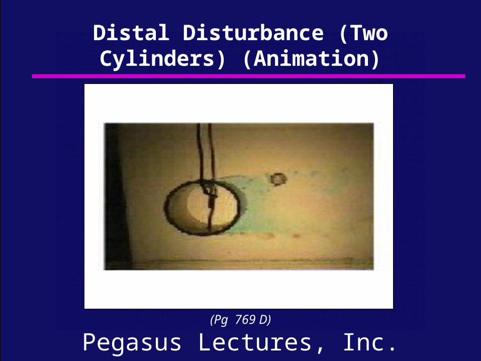
Distal Disturbance (Two Cylinders) (Animation)
(Pg 769 D)
Pegasus Lectures, Inc.
Add Title
Blank Slide:
This blank slide is here to help facilitate adding new content. If you would like to add material to this presentation, copy this slide and place in the correct location.