Embed Size (px)
Citation preview
12TH INTERNATIONAL DEPENDENCY AND STRUCTURE MODELLING CONFERENCE, DSM’10 22 – 23 JULY 2010, CAMBRIDGE, UK
PEM – A NEW MATRIX METHOD FOR SUPPORTING THE LOGIC PLANNING OF SOFTWARE DEVELOPMENT PROJECTS Zsolt Tibor Kosztyán and Judit Kiss University of Pannonia
Keywords: project scheduling, Dependency Structure Matrix (DSM), Stochastic Network Planning Method (SNPM), Project Expert Matrix (PEM)
1 INTRODUCTION Nowadays the notion of ’project’ is often used, however, it is important to make difference between projects. In the followings we make distinction between two groups. In the first group there are those projects (e.g construction projects) that follow the same technological order and building up from the same tasks according to a fixed order. In the second group there are projects requiring a more complexed planning (e.g. product development or software development projects), as the order of tasks can be handled in a more flexible way therefore the technological order is less fixed. In some cases the realisation of some functions/tasks can become uncertain due to time and/or resource constraint(s).
2 PROJECT SCHEDULING METHODS Network planning methods are mainly used for planning and scheduling projects (PMBOK, 2006). However, Critical Path Method (Kelley and Walker, 1959) and Metra Potential Method (or Precedence Diagramming Method) (Fondahl, 1961) can only handle tasks with given duration, the Program (or Project) Evaluation and Review Technique can handle stochastic durations (Fulkerson, 1962), while Graphical Evaluation and Review Technique can also handle decision events (Pritsker, 1966). These methods were developed for the scheduling of traditional projects, so at product or software development projects they can only be used partially or not at all, because these network planning methods cannot handle the specialities of these projects.
2.1 The principles of matrix methods The beginning of the development of network planning methods dates back to the 1950s, while matrix methods came to exist in the 1980s due to the work of Donald V. Steward. His Design/Dependency Structure Matrix (DSM) can be applied in different areas from system modelling to project scheduling; the practical application possibilities were primarily proven to be effective in case of product development projects (Steward, 1981). The rows and columns of the matrix show project tasks in the same order, and the marks in the matrix cells (with black or ’X’) refer to the precedence relations between tasks. Initially only the evidence of strict relations was marked with the help of DSM, but these did not provide any special information about the relation (dsmweb.org).
2.2 Improved matrix methods In case of the Numerical DSM (NDSM) the precedence relations are not just signed but also weighted according to different viewpoints. These relation/dependency weights could fall to different categories or in some cases (e.g. dependency strength) the weights are represented with numbers between 0 and 1. The bigger the value, the stronger the relation is. Primarily this method was developed for supporting system analyses or product development processes, later it was used for analysing and planning of projects as well (dsmweb.org). During a research at the University of Pannonia a new method was developed, namely Stochastic Network Planning Method (SNPM), which is independent from the NDSM. It is similar in appearance but different in semantics. In the SNPM the importance of a relation is represented with a value between 0 and 1. 0 shows a total independence, 1 shows certain relation, and the value between 0 and
97
1 shows uncertain or possible relation between tasks. If the values of cells are probabilities of the relation instead of the importance, it is signed with p(A,B)�[0,1] in case of tasks A and B, then 1-p(A,B) shows the probability that there is no relation between the two tasks. If 1-p(A,B)=p(A,B)=0,5, then the relation between these two tasks is indifferent, so the tasks can be realised sequentially and parallelly with the same probability (Kosztyán et al., 2008). Relations between tasks can be treated as probability if there are some a priori information about possible technological order from similar projects which were realised previously (in this case they are objective probabilities); or rather possible technological relations can be formed based on the opinions of different experts (in this case they are subjective probabilities). The diagonal does not play a role, so the values in the diagonal cells can be signed with 0 or with empty cells as well (Kosztyán et al., 2008). Since the relations are weighted according to their importance, it can be assumed that different graphs can be depicted from the matrix as a result. According to the importance of the relations it can be decided whether the realisation or the omission of the possible relation is more practical. Prior experience of similar projects, the constraints, the objective function (e.g. the most occurrence project scenario, minimal lead time, the least resource using, or combination of multiple objective functions) can influence this decision.
2.3 Specialities and application possibilities of PEM SNPM can be used in many cases, however, this method cannot handle all problems. For example in IT projects, especially in the case of software development it is possible that the order of some tasks can be reversed or tasks can be left out or replaced with other tasks (Kiss and Kosztyán, 2009a). These cases cannot be represented in SNPM, because this method can “only” handle the possible relations. We enhanced the SNPM and created the Project Expert Matrix (PEM). PEM can handle the possible occurrence of tasks as well, because the importance/probability of the task realisations can be represented in the diagonal of the matrix. Mark ‘X’ or 1 shows the certain tasks, the value between 0 and 1 shows the uncertain or possible tasks. If the values in the PEM diagonal show the (relative) priority/importance of the realisation and information about the cost, time and resource need are given, then the following exercise can be defined: A project scenario has to be determined that includes the most tasks within the given time, cost and resource limit. This process can be interesting in case of the so-called agile project planning that is used primarily at IT development projects (Kiss and Kosztyán, 2009b). In this paper we propose a solution to this problem. The agile project planning technique used at IT projects puts the concept of project management up-side-down. At the traditional project planning the goal of the realisation and the tasks are given, so the challenge is to determine the project scenario with the smallest cost, resource and time need. At agile projects the constraints are the time, the cost and the resources, while the goal is to realise as much of the tasks as possible (Dalcher, 2009). The agile project planning lacks a comprehensive support methodology as well as software support. It is difficult to use the traditional network planning methods, because they cannot handle the possible tasks. However, PEM can help the project experts to set the importance of the task realisation and to determine the omittable task. In the analysing phase of IT software development projects the so-called MoSCoW Analysis is a frequently applied method (Tierstein 1977). With MoSCoW Analysis those tasks/functions are defined that � have to be realised certainly, because it is the condition of the contract (Must have); � are not parts of the conditions of the contract, but they can be realized with a later modification, or
can contain useful functions (Should have); � although can be realized, but they require either too much cost/resources or too much time (Could
have). This analysis includes not only the tasks above (marked with M, S and C), but also those tasks, that will not realise in this project (Won’t have). Value 1 shows the certain tasks, value above 0.5 shows the tasks which have to be realized practically, value below 0.5 shows the omittable tasks and 0 shows the not-realising tasks in this project. It is possible to rank the tasks according to their importance.
98
The values of PEM can be calculated with taking logic plans of previous similar projects or experts’ opinions into account. If tasks are determined based on previous projects, then the occurrence probabilities of tasks are objective; and if the occurrence of tasks are determined based on the experts’ opinions, then the occurrence probabilities of tasks are subjective. At summarization of the different plans into PEM matrix it is practical to use the geometric mean instead of the arithmetic mean because of the independence of these opinions and experience. Diagonal values of PEM can be determined using votes employed in complex group decision making methods. These votes can be derived from the opinions of experts inside or outside of the company or from the stakeholders of prior projects as well. The votes can be calculated with equal or with different weights depending on various viewpoints (e.g. constraints or objective functions). Votes can be summarized with the help of complex group decision making methods, like KIPA or AHP (Analytic Hierarchy Process).
2.4 Determining possible logic plans from the PEM A two-step algorithm was developed to determine all possible deterministic solutions represented by the DSM matrices or in graphs which stem from the PEM that includes stochastic tasks and relations. The uncertainty of the PEM derives from the possibility of some tasks and relations, because a possible task and relation between tasks can be either realised, or not. If it is realised, then the occurrence probability of the project scenario is calculated with the value in the matrix (p), and if not then the occurrence probability is calculated with the complement (1-p). Firstly the PEM is regarded on the level of the tasks so all possible solutions have to be determined focusing on the values in the diagonal of the matrix. All possible combinations have to be created from the PEM, where each possible task can be realised (1) or not (0). This way SNPM matrices or project scenarios can be determined. Secondly SNPM matrices are regarded on the level of the precedence relations of which values are in the off-diagonal cells of the matrix. All possible combinations have to be created to each SNPM matrix to determine the case whether there is relation between two tasks (1) or whether there is not (0). These possible combinations can be represented with DSM matrices and/or representation graphs as well. In this way DSM matrices or project structures are determined. When determining the project scenarios it is necessary to define the tasks that have to be realised within a given time, cost and resource limit. It is the answer to the question: WHAT are those tasks which have to be realized in the course of the project. If the project scenario is determined, another question occurs: HOW, in what kind of logic order has the project be realised.
2.5 Selection methods Some algorithms were developed for ranking the possible solutions and choosing the best solutions. The Project Scenario/Structure Selection Method (PSSM) begins with the definition of tasks, and then they can be ranked according to their importance/probabilities in descending order. Since the tasks signed with 1 are the certain ones and the tasks with priority/probability 0 will not be realised, these tasks do not influence the number of possible project scenarios. It depends on the number of the uncertain/possible tasks (S and C). If it is k, then 2k is the number of possible project scenarios. The selecting process of the best project structure from the project scenarios is the same process as at PSSM. PEM can be extended, so more data can be depicted simultaneously assigning to the tasks (importance/probability, duration, resource and cost needs) and to the relations (importance, possible delay). If the exercise is to determine the logic plan with the highest priority/probability within a given time and resource limit, then time and resource needs are the constraints. The primary objective function is the determining of the project structure with the maximal (relative) priority/probability. The secondary objective function is selecting the project structure with the maximal (relative) priority within the time and resource constraints. The possible project scenario/project structure is determined with the help of PSSM method. A new agile project scheduling method (APS – Agile Project Scheduling) can take multiple objective functions into account at the same time, so it can determine the (optimal) resource allocation within time, cost and resource constraints.
99
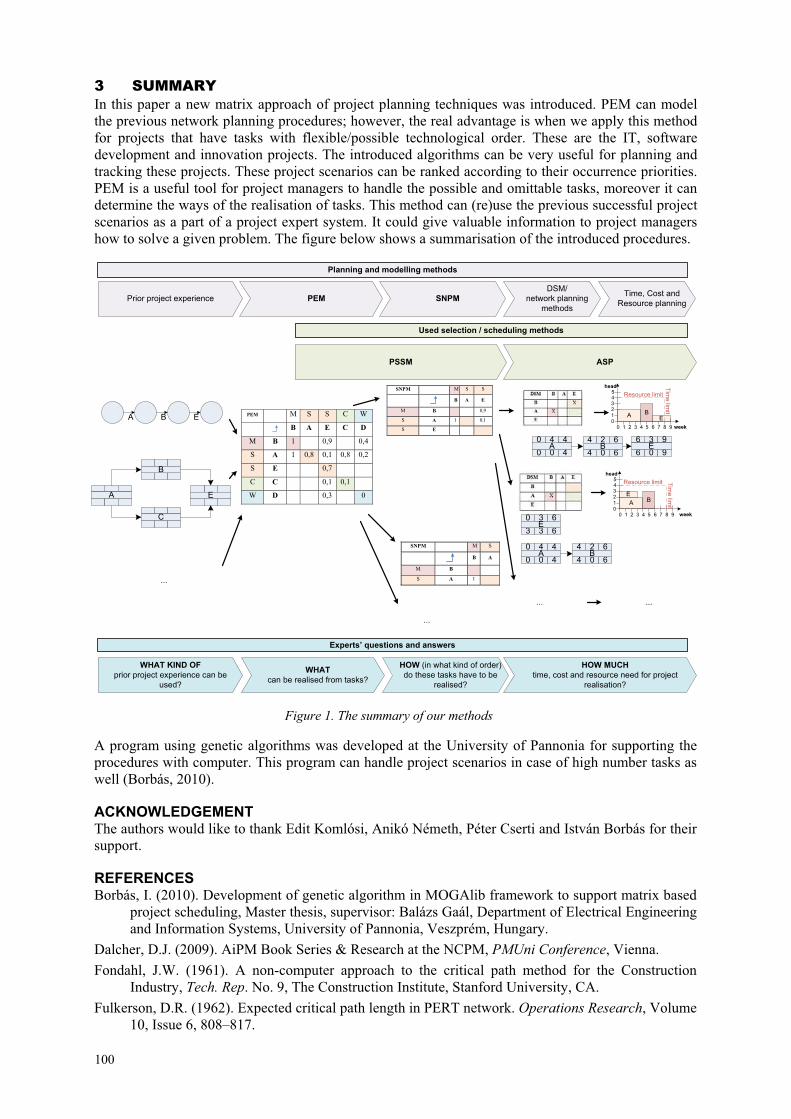
3 SUMMARY In this paper a new matrix approach of project planning techniques was introduced. PEM can model the previous network planning procedures; however, the real advantage is when we apply this method for projects that have tasks with flexible/possible technological order. These are the IT, software development and innovation projects. The introduced algorithms can be very useful for planning and tracking these projects. These project scenarios can be ranked according to their occurrence priorities. PEM is a useful tool for project managers to handle the possible and omittable tasks, moreover it can determine the ways of the realisation of tasks. This method can (re)use the previous successful project scenarios as a part of a project expert system. It could give valuable information to project managers how to solve a given problem. The figure below shows a summarisation of the introduced procedures.
Prior project experience PEM SNPMDSM/
network planning methods
Time, Cost and Resource planning
A B E
A
B
C
E
4 40 0 40
A2 6
4 0 64
B3 9
6 0 96
E
4 40 0 40
A2 6
4 0 64
B
3 63 3 60
E
0 1 2 3 4 5 6 7 8 9012345
week
head
A BE
Resource limit
Time lim
it
0 1 2 3 4 5 6 7 8 9012345
week
head
A BE
Resource limit Time lim
it
...
...
... ...
WHAT KIND OFprior project experience can be
used?
WHATcan be realised from tasks?
HOW (in what kind of order) do these tasks have to be
realised?
HOW MUCH time, cost and resource need for project
realisation?
SNPM M S S
B A E
M B 0,9
S A 1 0,1
S E
SNPM M S
B A
M B
S A 1
PEM M S S C W
B A E C D
M B 1 0,9 0,4
S A 1 0,8 0,1 0,8 0,2
S E 0,7
C C 0,1 0,1
W D 0,3 0
ASP
Used selection / scheduling methods
Experts’ questions and answers
Planning and modelling methods
PSSM
...
Figure 1. The summary of our methods
A program using genetic algorithms was developed at the University of Pannonia for supporting the procedures with computer. This program can handle project scenarios in case of high number tasks as well (Borbás, 2010).
ACKNOWLEDGEMENT The authors would like to thank Edit Komlósi, Anikó Németh, Péter Cserti and István Borbás for their support.
REFERENCES Borbás, I. (2010). Development of genetic algorithm in MOGAlib framework to support matrix based
project scheduling, Master thesis, supervisor: Balázs Gaál, Department of Electrical Engineering and Information Systems, University of Pannonia, Veszprém, Hungary.
Dalcher, D.J. (2009). AiPM Book Series & Research at the NCPM, PMUni Conference, Vienna. Fondahl, J.W. (1961). A non-computer approach to the critical path method for the Construction
Industry, Tech. Rep. No. 9, The Construction Institute, Stanford University, CA. Fulkerson, D.R. (1962). Expected critical path length in PERT network. Operations Research, Volume
10, Issue 6, 808–817.
100
Kelley Jr., J.E. and Walker, M.R. (1959). Critical Path Planning and Scheduling: An Introduction. Mauchly Associates, Ambler, PA.
Kiss, J. and Kosztyán, Zs.T. (2009a). The importance of logic planning in case of IT and innovation projects, AVA (International Congress on the Aspects and Vision of Applied Economics and Informatics), Debrecen.
Kiss, J. and Kosztyán, Zs.T. (2009b). Handling the Specialties of Agile IT Projects with a New Planning Method, CONFENIS (The Enterprise Information Systems International Conference on Research and Practical Issues of EIS), Gy�r, Hungary.
Kosztyán, Zs.T., Fejes, J. and Kiss, J. (2008). Handling stochastic network structures in project scheduling, Szigma XXXIX. pp. 85-103.
MIT DSM Research Group (2005). MIT DSM Web Site, http:// www.dsmweb.org/ Pritsker, A.A. (1966). GERT: Grafical Evaluation and Review Technique, MEMORANDUM, RM-
4973-NASA. Project Management Institute (2006). A Guide to the Project Management Body of Knowledge
(PMBOK® Guide – 3rd Edition), ISBN 963 05 8401 8. Steward, D. (1981). System Analysis and Management: Structure, Strategy, and Design, New York:
Petrocelli Books Tierstein, L.M. (1997). Managing a Designer/2000 Project. New York Oracle User Group. Fall ’97.
http://www.wrsystems.com/whitepapers/managedes2k.pdf. Retrieved 2008-05-31.
Contact: Judit Kiss University of Pannonia Department of Management Egyetem utca 10. 8200 Veszprém Hungary Phone: +36/88/624-243 Fax: +36/88/624-524 E-mail: [email protected]
101
BY MODELLING DEPENDENCIESMANAGING COMPLEXITY
PEM – A New Matrix Method for Supporting the Logic Planning of Software Development Projectsp j
Zsolt Tibor KosztyánJudit KissJudit Kiss
University of Pannonia, Hungary
BY MODELLING DEPENDENCIESMANAGING COMPLEXITY
IndexIndex
• Specialities of IT projects
f• Process of traditional project planning
• Agile project management approach
for supporting IT projects
• Storing prior project experience
• How can values of the PEM be determined?
• Selecting the tasks
• Sharing prior project experience
• Selecting the optimal solution
• An existing, practical IT project
• Results – Using genetic algorithm
12th International DSM Conference 2010- 2
Results Using genetic algorithm• Summary
102
BY MODELLING DEPENDENCIESMANAGING COMPLEXITY
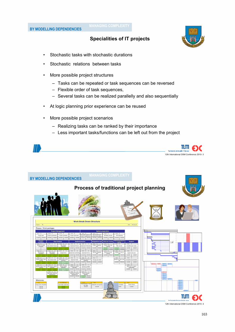
Specialities of IT projectsSpecialities of IT projects
• Stochastic tasks with stochastic durations
• Stochastic relations between tasks
• More possible project structures
– Tasks can be repeated or task sequences can be reversed– Flexible order of task sequences– Flexible order of task sequences,– Several tasks can be realized parallelly and also sequentially
• At logic planning prior experience can be reused• At logic planning prior experience can be reused
• More possible project scenarios
– Realizing tasks can be ranked by their importance– Less important tasks/functions can be left out from the project
12th International DSM Conference 2010- 3
BY MODELLING DEPENDENCIESMANAGING COMPLEXITY
Process of traditional project planningProcess of traditional project planning
Work Break Down StructureProject: Date: 2010,05,29
Phases / Work packages
4.1.1 4.1.3 4.1.4 4.1.5 4.2.2 4.2.3 4.2.4 4.2.5
17,12,07 18,01,08 14,01,08 13,06,08 14,01,08 13,06,08 02,06,08 13,06,08 20,12,07 28,01,08 15,01,08 28,03,08 14,01,08 13,06,08 15,01,08 15,03,08
Project close down SAP AuthorithyProject controllingProject coordination SAP Basis services
System preparation
Project startCheck SAP readiness of local IT infrastructure
Z…
Project Management
Plan & build local IT infrastructure updates
4.3.1 4.4.1 A 4.4.6 F 4.5.1 A 4.5.6 F 4.6.1 4.7.1 4.8.1 4.9.1
- - 28,01,08 28,02,08 28,01,08 28,02,08 25,02,08 04,04,08 25,02,08 04,04,08 31,03,08 04,04,08 04,02,08 21,03,08 22,02,08 04,04,08 12,05,08 13,06,0828,01,08 29,02,08 28,01,08 29,02,08 04,02,08 in progress 22,02,08 in progress
4.3.2 4.4.2 B 4.4.7 G 4.5.2 B 4.5.7 G 4.6.2 4.7.2 4.8.2 4.9.2
14,01,08 25,01,08 28,01,08 28,02,08 28,01,08 28,02,08 25,02,08 04,04,08 25,02,08 04,04,08 07,04,08 11,04,08 21,04,08 30,05,08 04,03,08 30,03,08 12,05,08 13,06,0814 01 08 25 01 08 28 01 08 29 02 08 28 01 08 29 02 08
(End) User Training
Implement Finance
Execute integration test
Prepare (End) user training
Implement Production
Final preparation & go liveImplementation
Plan cut over
Prepare & Test cut over
Execute end user training
Gap Analysis
Design formsGap analysis Controlling
Gap analysis Production
Implement FormsImplement Controlling
Initialize template processes
Gap analysis Finance
Support
Prepare integration test
Integration testProject enabling
Briefing local consultants
Support end users
Complete open issues
14,01,08 25,01,08 28,01,08 29,02,08 28,01,08 29,02,08
4.3.3 4.4.3 C 4.4.8 H 4.5.3 C 4.5.8 H 4.6.3 4.8.3 4.9.3
14,01,08 25,01,08 28,01,08 28,02,08 20,02,08 07,03,08 25,02,08 04,04,08 25,02,08 04,04,08 14,04,08 18,04,08 01,05,08 09,05,08 12,05,08 13,06,0814,01,08 25,01,08 28,01,08 29,02,08 28,01,08 in progress
4.3.4 4.4.4 D 4.4.9 I 4.5.4 D 4.5.9 I 4.9.4
15,01,08 25,01,08 28,01,08 28,02,08 28,01,08 07,03,08 25,02,08 04,04,08 25,02,08 04,04,08 02,06,08 13,06,0815,01,08 25,01,08 28,01,08 29,02,08 28,01,08 in progress
4.4.5 E 4.5.5 E 4.5.10 J
Implement Logistic Execution
Implement add ons & interfaces
Ch R t
Interfacing RAMIR
Implement SalesDesign add ons and interfaces
Execute cut over & go-live
Fix bugs and retestGap analysis SalesPrepare Project Team Training
G l i M t i l I l t M t i l
Hand over to support organization
Gap analysis Logistic execution
Design RAMIR integration
Complete documentation
Execute Project Team Training
28,01,08 28,02,08 25,02,08 04,04,08 25,02,08 04,04,0828,01,08 29,02,08 25,02,08 in progress
Milestones4.1.6
Change Request Handling
29,02,0818,04,08
4.8.4
Go live completed
4.6.4
04,04,08
4.1.2 4.4.10 Mile Stone
Gap analyis Materials Management
15,01,08
Gap designs approvedProject start completed
09,05,08
Implementation ready for I-test
Implement Material Management
4.5.11
15,01,08 28,02,08
Integration test passed
13,06,08
Project closed
12th International DSM Conference 2010- 4
103

BY MODELLING DEPENDENCIESMANAGING COMPLEXITY
Agile project management approach for supporting IT projects
j gTraditional
project planning gAgile project
planning
Scope Time BudgetFixed
Time Budget ScopeVariable
12th International DSM Conference 2010- 5
Time
(Dalcher, 2009)
BY MODELLING DEPENDENCIESMANAGING COMPLEXITY
Storing prior project experienceStoring prior project experience
Project Project ExpertExpert MatrixMatrix
PEM A B C D E
A 1 0.9 0.7 0.3 0
B 0 0.8 0.4 0.6 0.25
C 0 0 1 0.5 0.5
D 0 0 0 0.3 1
E 0 0 0 0 1
12th International DSM Conference 2010- 6
…104
BY MODELLING DEPENDENCIESMANAGING COMPLEXITY
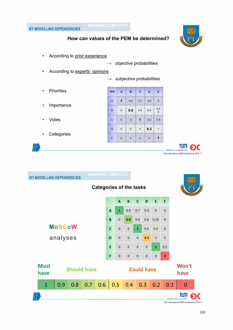
How can values of the PEM be determined?How can values of the PEM be determined?
• According to prior experience• According to prior experience� objective probabilities
• According to experts’ opinionsAccording to experts opinions� subjective probabilities
P i iti• Priorities
• Importance
PEM A B C D E
A 1 0.9 0.7 0.3 0
Importance
• Votes
B 0 0.8 0.4 0.6 0.25
C 0 0 1 0.5 0.5
• CategoriesD 0 0 0 0.3 1
E 0 0 0 0 1
12th International DSM Conference 2010- 7
BY MODELLING DEPENDENCIESMANAGING COMPLEXITY
Categories of the tasks
A B C D E F
Categories of the tasks
A 1 0.9 0.7 0.3 0 0
B 0 0.8 0.4 0.6 0.25 0
C 0 0 1 0.5 0.5 0
D 0 0 0 0 3 1 0
MoSCoW
analyses D 0 0 0 0.3 1 0
E 0 0 0 0 1 0,3
F
analyses
MMust h
SShould have CCould haveWWon't h
F 0 0 0 0 0 0
have have
1 0.9 0.8 0.7 0.6 0.5 0.4 0.3 0.2 0.1 0
12th International DSM Conference 2010- 8
105

BY MODELLING DEPENDENCIESMANAGING COMPLEXITY
Sequentially or parallelly?Sequentially or parallelly?
M 1
A B C D E S0.90.80.7STi Tj
Ti ?A 1 0.9 0.7 0.3 0
B 0 0.8 0.4 0.6 0.25
0.70.60.5
S
TjC 0 0 1 0.5 0.5
D 0 0 0 0.3 1
C 0.40.30.2
E 0 0 0 0 1
W
0.20.10
12th International DSM Conference 2010- 9
BY MODELLING DEPENDENCIESMANAGING COMPLEXITY
Selecting the tasksSelecting the tasksStep 1
B d tBudget
……
12th International DSM Conference 2010- 10
Selected tasks: A, C, E, B, D
106
BY MODELLING DEPENDENCIESMANAGING COMPLEXITY
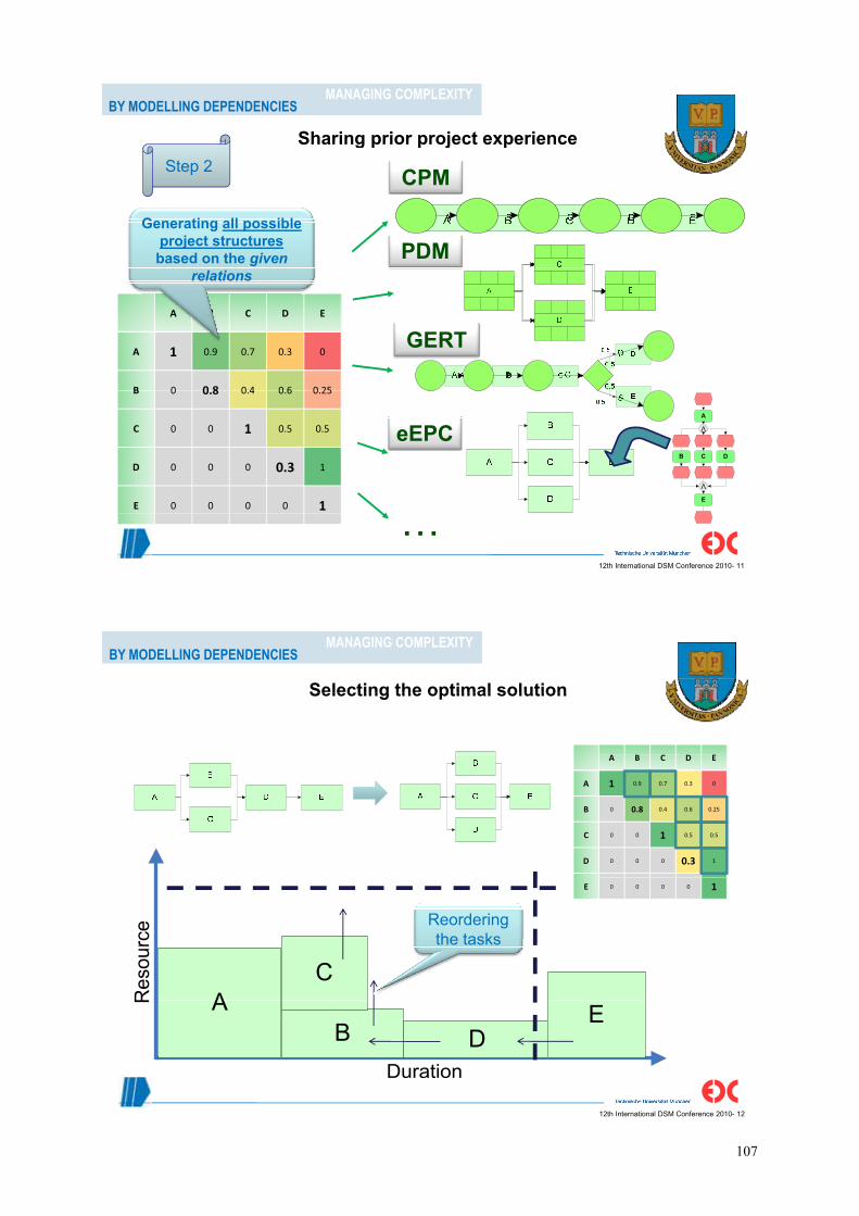
Sharing prior project experienceg p p j p
CPMStep 2
PDMGenerating all possible
project structures based on the given
A B C D E
relations
GERTA 1 0.9 0.7 0.3 0
B 0 0 8 0 4 0 6 0 25
eEPC
B 0 0.8 0.4 0.6 0.25
C 0 0 1 0.5 0.5A
V
D 0 0 0 0.3 1
E 0 0 0 0 1
DB C
V
E
12th International DSM Conference 2010- 11
…
BY MODELLING DEPENDENCIESMANAGING COMPLEXITY
Selecting the optimal solutionSelecting the optimal solution
A B C D E
A 1 0.9 0.7 0.3 0
B 0 0.8 0.4 0.6 0.25
C 0 0 1 0.5 0.5
D 0 0 0 0.3 1
E 0 0 0 0 1
Reorderingthe tasksthe tasks
12th International DSM Conference 2010- 12
107
BY MODELLING DEPENDENCIESMANAGING COMPLEXITY
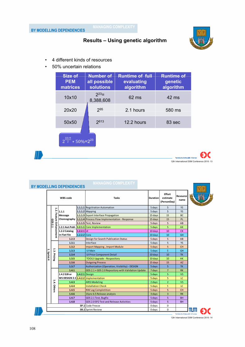
Results – Using genetic algorithmResults Using genetic algorithm
4 diff t ki d f• 4 different kinds of resources• 50% uncertain relations
Size of Number of Runtime of full Runtime ofSize of PEM
matrices
Number of all possiblesolutions
Runtime of fullevaluatingalgorithm
Runtime of genetic
algorithm223=10x10 223=
8,388,608 62 ms 42 ms
20x20 295 2.1 hours 580 ms20x20 2 2.1 hours 580 ms
50x50 2613 12.2 hours 83 sec
�����
� � ���=223
12th International DSM Conference 2010- 13
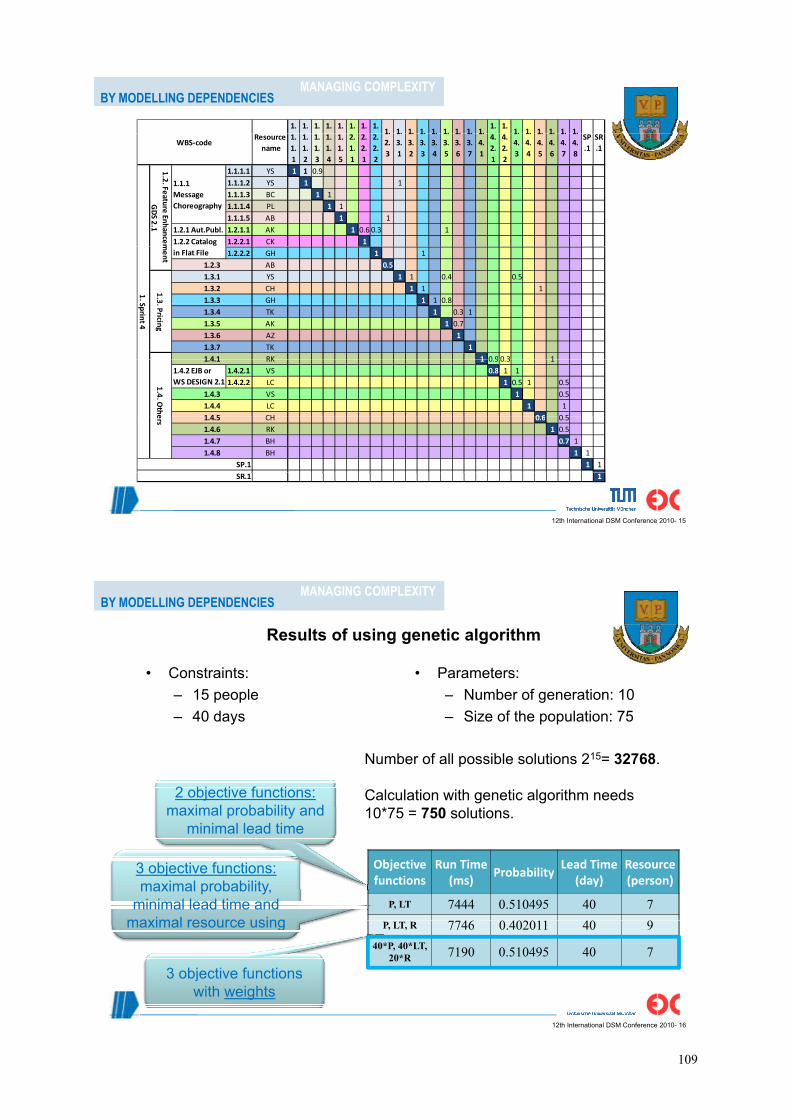
BY MODELLING DEPENDENCIESMANAGING COMPLEXITY
Tasks DurationEffort
estimateResource
WBS code Tasks Duration estimate (PersonDay)
name
1.1.1.1 Regsitration Automation 5 days 5 YS1.1.1.2 Mapping 5 days 5 YS1 1 1 3 Export Interface Propagation 15 days 15 BC
WBS-code
1.1.1 Message
1.2. Fe
1.1.1.3 Export Interface Propagation 15 days 15 BC1.1.1.4 Process Flow Implementation - Response 15 days 15 PL1.1.1.5 Test, Review 5 days 5 AB
1.2.1 Aut.Publ. 1.2.1.1 Core Implementation 5 days 5 AK1.2.2.1 UI 10 days 10 CK
Message Choreography
1.2.2 Catalog
eature Enhance mG
DS 2.1
1.2.2.2 Core 10 days 10 GHDesign for Search Publication Status 5 days 5 ABInterface 5 days 5 YSImport Mapping , Import Module 5 days 5 CHUI M i 5 d 5 GH
1 .1
1.3.11.3.21 3 3
in Flat File
ment
1.2.3
UI Main 5 days 5 GH UI Price Component Detail 10 days 10 TK TOOLS Upgrade - Respository 10 days 10 AKOutgoing Process 15 days 15 AZAuthorization (Operation, Visibility) - DESIGN 5 days 5 TK
.3. Pricing
. Sprint 4
1.3.31.3.41.3.51.3.61.3.7 ( p y) y
GDS 2.1 + GDS 2.0 Repository with Validation Update 7 days 7 RK1.4.2.1 Design 5 days 5 VS1.4.2.2 Implementation 5 days 5 LC
ARIS Modeling 2 days 2 VSI ll i Ch k 5 d 5 LC
1.4.1
1.4.31 4 4
1.4.2 EJB or WS DESIGN 2.11.4. O
Installation Check 5 days 5 LCNW Log Completition 5 days 5 CH1Sync 6.5 Release analysis 3 days 3 RKGDS 2.1 Test, Bugfix 5 days 5 BHGDS 2.0 SP2 Test and Release Activities 5 days 5 BH1.4.8
1.4.41.4.51.4.61.4.7
Others
12th International DSM Conference 2010- 14
yCode Freeze 0 days 0Sprint Review 0 days 0
SP.1SR.1
108
BY MODELLING DEPENDENCIESMANAGING COMPLEXITY
1. 1. 1. 1. 1. 1. 1. 1.1. 1. 1. 1. 1. 1. 1. 1. 1.
1. 1.1. 1. 1. 1. 1. 1.
Resource name
1.1.1
1.1.2
1.1.3
1.1.4
1.1.5
2.1.1
2.2.1
2.2.2
1.2.3
1.3.1
1.3.2
1.3.3
1.3.4
1.3.5
1.3.6
1.3.7
1.4.1
4.2.1
4.2.2
1.4.3
1.4.4
1.4.5
1.4.6
1.4.7
1.4.8
SP.1
SR.1
1.1.1.1 YS 1 1 0.91.1.1.2 YS 1 1
WBS-code
1.1.1
1.2. F
1.1.1.3 BC 1 11.1.1.4 PL 1 11.1.1.5 AB 1 1
1.2.1 Aut.Publ. 1.2.1.1 AK 1 0.6 0.3 11.2.2.1 CK 1
Message Choreography
1.2.2 Catalog
eature Enhance mG
DS 2.1
1.2.2.2 GH 1 1AB 0.5YS 1 1 0.4 0.5CH 1 1 1GH 1 1 0.8
1. 3
1. S
1.3.11.3.21.3.3
in Flat File
ment
1.2.3
TK 1 0.3 1AK 1 0.7AZ 1TK 1RK 1 0 9 0 3 11 4 1
3. Pricing
Sprint 4
1.3.41.3.51.3.61.3.7
RK 1 0.9 0.3 11.4.2.1 VS 0.8 1 11.4.2.2 LC 1 0.5 1 0.5
VS 1 0.5LC 1 1CH 0 6 0 5
1.4.1
1.4.31.4.41 4 5
1.4.2 EJB or WS DESIGN 2.11.4. O
the
CH 0.6 0.5RK 1 0.5BH 0.7 1BH 1 1
1 11.4.8
SP.1
1.4.51.4.61.4.7
ers
12th International DSM Conference 2010- 15
1SR.1
BY MODELLING DEPENDENCIESMANAGING COMPLEXITY
Results of using genetic algorithmResults of using genetic algorithm
• Constraints:15 people
• Parameters:Number of generation: 10– 15 people
– 40 days– Number of generation: 10– Size of the population: 75
2 objective functions: i l b bilit d
Number of all possible solutions 215= 32768.
Calculation with genetic algorithm needs 10* 0 l i
Objective Run Time Lead Time Resource
maximal probability and minimal lead time
3 bj ti f ti
10*75 = 750 solutions.
Objective functions
Run Time (ms)
ProbabilityLead Time
(day)Resource (person)
P, LT 7444 0.510495 40 746 0 402011 40 9
3 objective functions: maximal probability,
minimal lead time and maximal resource using P, LT, R 7746 0.402011 40 9
40*P, 40*LT, 20*R 7190 0.510495 40 7
maximal resource using
3 objective functions
12th International DSM Conference 2010- 16
3 objective functionswith weights
109
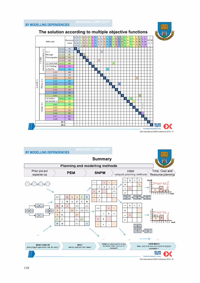
BY MODELLING DEPENDENCIESMANAGING COMPLEXITY
The solution according to multiple objective functionsg p j
Resource name
1.1.1.1
1.1.1.2
1.1.1.3
1.1.1.4
1.1.1.5
1.2.1.1
1.2.2.1
1.2.2.2
1.2.3
1.3.1
1.3.2
1.3.3
1.3.4
1.3.5
1.3.6
1.3.7
1.4.1
1.4.2.1
1.4.2.2
1.4.3
1.4.4
1.4.5
1.4.6
1.4.7
1.4.8
SP.1
SR.1
WBS-code
1.1.1.1 YS 1 1 1.1.1.2 YS 1 1 1.1.1.3 BC 1 1 1.1.1.4 PL 1 1 1.1.1.5 AB 1 1
1.2. Feature En hG
DS 2 .
1.1.1 Message Choreography
1.2.1 Aut.Publ. 1.2.1.1 AK 1 1 . 11.2.2.1 CK 1 1.2.2.2 GH 1 1
AB 1 YS 1 1 . .
hancement
.1
1.2.2 Catalog in Flat File
1.2.31.3.1
CH 1 1 1 GH 1 1 . TK 1 . 1 AK 1 . AZ 1 1.3.6
1. Sprint 4
1.3. Pricing
1.3.21.3.31.3.41.3.5
TK 1 RK 1 1
1.4.2.1 VS 1 1 1 1.4.2.2 LC 1 1 .
VS 1 1
1.3.7
1.4
1.4.11.4.2 EJB or WS DESIGN 2.1
1.4.3LC 1 1 CH 1 . RK 1 1 BH 1 1 BH 1 1
. Others
1.4.41.4.51.4.61.4.71.4.8
12th International DSM Conference 2010- 17
BH 1 1 1 1 1
SP.1SR.1
1.4.8
BY MODELLING DEPENDENCIESMANAGING COMPLEXITY
Summary
SNPM M S S
� B A E
DSM B A E
B X
A XM B 0.9
S A 1 0.1
S E
PEM M S S C W
� B A E C D
E
M B 1 0.9 0.4
S A 1 0.8 0.1 0.8 0.2
S E 0.7
SNPM M S
� B A
B
DSM B A E
B
A X
C C 0.1 0.1
W D 0.3 0
M B
S A 1
E
12th International DSM Conference 2010- 18
110