Embed Size (px)
Citation preview

Percolation, statistical topography, and transport in random media
M. B. Isichenko
institute for Fusion Studies, The University of Texas at Austin, Austin, Texas 78712and Kurchatov Institute ofAtomic Energy, 129182 Moscow, Russia
A review of classical percolation theory is presented, with an emphasis on novel applications to statisticaltopography, turbulent diffusion, and heterogeneous media. Statistical topography involves the geometri-cal properties of the isosets (contour lines or surfaces) of a random potential f(x). For rapidly decayingcorrelations of g, the isopotentials fall into the same universality class as the perimeters of percolationclusters. The topography of long-range correlated potentials involves many length scales and is associatedeither with the correlated percolation problem or with Mandelbrot's fractional Brownian reliefs. In allcases, the concept of fractal dimension is particularly fruitful in characterizing the geometry of randomfields. The physical applications of statistical topography include diffusion in random velocity fields, heatand particle transport in turbulent plasmas, quantum Hall effect, magnetoresistance in inhomogeneousconductors with the classical Hall effect, and many others where random isopotentials are relevant. Ageometrical approach to studying transport in random media, which captures essential qualitative featuresof the described phenomena, is advocated.
CONTENTSI. Introduction
A. GeneralB. Fractals
II. PercolationA. Lattice percolation and the geometry of clustersB. Scaling and distribution of percolation clustersC. The universality of critical behaviorD. Correlated percolationE. Continuum percolation
III. Statistical TopographyA. Spectral description of random potentials and Gaussi-
anityB. Brownian and fractional Brownian reliefsC. Topography of a monoscale relief
1. Two dimensions2. Three dimensions
D. Monoscale relief on a gentle slopeE. Multiscale statistical topography
1. Two dimensions2. Three dimensions3. Correlated cluster density exponent4. An example: Potential created by disordered
charged impurities5. DifBculties of the method of separated scales
F. Statistics of separatricesIV. Transport in Random Media
A. Advective-diffusive transport1. When is the effective transport diffusive, and what
are the bounds on effective diffusivity?2. Effective diffusivity: Simple scalings3. Diffusion in two-dimensional random, steady flows4. Lagrangian chaos and Kolmogorov entropy5. Diffusion in time-dependent random flows6. Anomalous diffusion
a. Superdiffusionb. Subdiffusion
B. Conductivity of inhomogeneous media1. Keller-Dykhne reciprocity relations2. Systems with inhomogeneous anisotropy
a. Polycrystalsb. Plasma heat conduction in a stochastic mag-
netic field
3. Magnetoresistance of inhomogeneous media with
961961963967968976977978979984
985988992992994994996997999999
10001000100110021003
100410051008101010131016101610191022102210241024
1026
the Hall effecta. The method of reciprocal mediab. Determination of effective conductivity using
an advection-diffusion analogyC. Classical electrons in disordered potentials
V. Concluding remarksAcknowledgmentsReferences
10271028
102810301033103310331033
I. INTRODUCTION
A. General
The percolation problem describes the simplest possi-ble phase transition with nontrivial critical behavior.The pure geometrical nature of this transition and itscompelling application to diverse physical problems havedrawn the attention of many researchers, and the per-colation theory is well reviewed (Shante and Kirkpatrick,1971; Essam, 1972; Kirkpatrick, 1973; Stauffer, 1979; Es-sarn, 1980; Kesten, 1982; Deutscher et al. , 1983; Zallen,1983; Shklovskii and Efros, 1984; Stauffer, 1985; Sokolov,1986). The general formulation of the percolation prob-lem is concerned with elementary geometrical objects(spheres, sticks, sites, bonds, etc. ) placed at random in ad-dimensional lattice or continuum. The objects have awell-defined connectivity radius A,o, and two objects aresaid to communicate if the distance between them is lessthan A,o. One is interested in how many objects can forma cluster of communication and, especially, when andhow the clusters become infinite. The control parameteris evidently the density no of the objects (their averagenumber per unit volume), or the dimensionless filling fac-tor g=npk, o. The percolation threshold, g=g„corre-sponds to the minimum concentration at which aninfinite cluster spans the space Thus the. percolationmodel exhibits two essential features: critical behaviorand long-range correlations near the critical value of the
Reviews of Modern Physics, Vol. 64, No. 4, October 1992 Copyright 1992 The American Physical Society 961

962 M. B. Isichenko: Percolation, statistical topography, and transport in random media
control parameter q.This model is relevant for a number of transport prob-
lems in disordered media exhibiting critical behavior,such as electron localization (Anderson, 1958; Ziman,1969) and hopping conduction in amorphous solids (Zal-len, 1983; Shklovskii and Efros, 1984). Other applica-tions of percolation theory may concern the spreading ofdisease in a garden or, say, the critical concentration ofbribe takers to impede the normal functioning of agovernment.
Not only critical phenomena can be associated withthe percolation model. Consider, for example, thediffusion of a passive tracer in a two-dimensional, steady,incompressible random fIow
tion transition enter the result because the large value ofthe control parameter (I' ))1) picks up a near-critical (inthe sense of the contour percolation) set of streamlinesdominating the effective transport. Unlike the transportprocesses occurring on the percolation clusters (Aharony,1984; Orbach, 1984; Rammal, 1984; O'Shaughnessy andProcaccia, 1985a, 1985b; Hans and Kehr, 1987; Harris,1987; Havlin and Ben-Avraham, 1987), the motion alongincompressible streamlines represents transport aroundthe percolation clusters.
The appearance of formula (1.3) leaves little hope forits derivation using a regular perturbation-theory methodin solving the advection-diffusion equation
v(x, y) =Vg(x, y) Xz, Bn
at+vVn=D Vn (1.4)
where g(x,y) is a random stream function. The stream-lines of this Sow are the contours of P. The geometry ofthe streamlines is associated with the geometry of per-colation clusters as follows. Let us call "objects" the re-gions where g(x,y) is less than a specified constant levelh. If z =f(x,y) is imagined to be the elevation of a ran-dom landscape and h designates the level of Aooding,then the objects are the lakes. Two neighboring lakes"communicate" if they merge into a bigger lake, which isa "cluster. " So the contours g(x,y) =h present the coast-lines of the lakes, that is, the envelopes of the clusters.The control parameter of this percolation problem is thelevel h such that at some critical level, h =h„ the lakesform an infinite ocean and among the contoursg(x,y) = Ii, there is at least one infinitely long.
Flow (1.1), however, includes streamlines lying at alllevels, and its transport properties show no critical be-havior in the only relevant control parameter (Pecletnumber)
0P=0
(1.2)
which is the ratio of the root-mean-square stream func-tion $0 and the molecular diffusivity Do of the tracer.Nevertheless, if the Peclet number is large, P))1, thetransport shows long correlation because the tracer parti-cles advected along very large streamlines diffuse veryslowly from these lines to more typical short closed linesand hence provide a significant coherent contribution tothe turbulent diffusivity D*. The larger the Peclet num-ber, the longer and narrower the bundles of streamlinesthat dominate the effective transport in the consideredAow. Under certain constraints, the effective diffusivityscales as (Isichenko et al. , 1989)
D*=D0P' ', P ))1, (1.3)
where the exponent 10/13 is expressible in terms of thecritical exponents of two-dimensional percolation theory(Sec. IV.A.3).
The effective diffusion in a random Aow presents an ex-ample of a long-range correlated phenomenon withoutcritical behavior. The critical exponents of the percola-
for the tracer density n. Instead, geometrical argumentscan be used to reduce the advective-diffusive problem tothe problem of random contours, whose critical behavioris not amenable to any kind of a perturbation analysis butis well described in terms of percolation theory.
The problem of critical phenomena (cf. Domb et al.1972—1988) is among the most difficult in nonlinearphysics. This is well manifested by the fact that severaldecades separate the Boltzmann-Gibbs statisticalmechanics and the first solution of the Ising model byOnsager (1944). After Wilson (1971a, 1971b, 1975) intro-duced the renormalization-group technique to the theoryof phase transitions, the number of solvable critical mod-els rapidly increased (Ma, 1976; Baxter, 1982). Some ofthe analytical results on percolation criticality were ob-tained relatively recently (den Nijs, 1979; Saleur and Du-plantier, 1987).
The value of the available results on critical behaviorsis grossly increased by the universality of critical exponents describing the behavior of the order parameterand of other physical quantities near the critical point(Sec. II.C). Universality implies that the set of criticalexponents is structurally stable —that is, it does notchange under a small perturbation of the model itself,provided that the perturbation does not introduce longcorrelations that decay slower than certain algebraicfunctions. This universality leads to the possibility ofnew applications of critical phenomena theory that mightgo far beyond the phase-transition problems in statisticalphysics.
There exists a class of problems of transport in randomand disordered media that can be reduced to the statisti-cal properties of contours (isolines or isosurfaces) of ran-dom potentials. The geometrical properties of randomisosets are studied in the framework of statistical topogra-phy (Ziman, 1979; Isichenko and Kalda, 1991b). In thesimplest case of a potential characterized by a single scaleof length and a rapidly decaying correlation function, thestatistical topography problem can be mapped onto thestandard percolation problem, where the random con-tours are associated with percolation perimeters (Secs.II.E and III.C). In two dimensions the basic percolation
Rev. Mod. Phys. , Vol. 64, No. 4, October 1992

M. B. lsichenko: Percolation, statistical topography, and transport in random media 963
exponents are known exactly (Sec. II.A), thereby present-ing all necessary characteristics of the long-range contourbehavior. For the case of algebraic behavior in the ran-dom potential correlator, the topography involves essen-tially many length scales, but still can be studied usingthe formalism of fractional Brownian functions (Sec.III.B), the long-range correlated percolation problem(Sec. II.D), or a renormalization-group-style technique ofthe separation of scales (Sec. III.E) built on the knowledgeof the monoscale percolation exponents.
The paper concentrates on various physical applica-tions of percolation theory and statistical topography,such as the quantized Hall conductance (Secs. III.D andIII.E.4) and the processes of transport in classical ran-dom media, including advection-diff'usion transport (Sec.IV.A) or inhomogeneous conductors (Sec. IV.B). TheAows discussed in the context of advection-diffusion arenot necessarily of hydrodynamic origin. The focus ofSecs. IV.A.4 and IV.A.5 is primarily on transport in tur-bulent plasmas, including the diffusion of stochasticmagnetic-field lines and charged particles, whereas Sec.IV.B.3.b deals with an electrostatic potential advected byabstract (nonphysical) flows, a problem arising when theeffective conductivity of inhomogeneous media (polycrys-tals, for example) in a strong magnetic field is calculated.
The outline of the paper is presented by the table ofcontents, and so is not repeated here. Two remarks re-garding the organization of the review are in order, how-ever. Section I.B serves as a terse introduction to thefractal geometry that is heavily used throughout the pa-per. Those readers who are familiar with fractals maywish to skip this discussion. It is included here, since incertain quarters —for example, in the plasma physicscommunity —fractals are, regrettably, scarcely used andthe necessity to refer to the original texts would makethis paper difficult to read. Secondly, it should be notedthat Sec. II adds to the existing excellent reviews of per-colation theory (Stauffer, 1979; Essam, 1980; Deutscheret a/. , 1983; Zallen, 1983; Shklovskii and Efros, 1984;Stauff'er, 1985) only a moderate amount of new discussionregarding the problems of correlated percolation (Sec.II.D) and continuum percolation (Sec. II.E). Readers fa-miliar with percolation theory may wish to begin withSec. III.
B. Fractals
An essentially geometrical approach to studying trans-port processes requires a concise characterization of ran-dom fields. The fractal dimension serves such a purpose.Introduced originally by Hausdorff (1918) and Besicov-itch (1929), the concept of fractional, or generalized, di-mension was first used in fairly abstract mathematicalstudies on number theory (Besicovitch, 1935a, 1935b;Good, 1941). The fractal dimension was introduced in aphysical context by Mandelbrot (1975a, 1977, 1982,1983), whose works generated a widespread interest in
fractal geometry (Pietronero and Tosatti, 1986; Paladinand Vulpiani, 1987; Feder, 1988; Peitgen and Saupe,1988; Voss, 1989). Fractal dimensions were reported fornumerous environmental data (Burrough, 1981) and evenfor space-time (Zeilinger and Svozil, 1985). The mostsensible physical applications of fractals are concernedwith fluid turbulence (Mandelbrot, 1975b; Procacia,1984; Sreenivasan and Meneveau, 1986; Benzi et al. ,1991;Constantin et al. , 1991),chaotic attractors (Kaplanand Yorke, 1979; Mori, 1980; Farmer et al. , 1983;Grassberger and Procaccia, 1983), electron localization(Levy and Souillard, 1987), and critical phenomena(Suzuki, 1983), including the transition to chaos in classi-cal systems (Jensen et al. , 1985). Of course, there aremany others (Mandelbrot, 1983; Feder, 1988; Falconer,1990; Bunde and Havlin, 1991).
We begin our discussion of fractals with somewhatabstract mathematical definitions to be followed by morespecific physical examples. The original Hausdorff-Besicovitch definition of the "dimensional number" D ofa set of points F embedded in a d-dimensional space is asfollows. Let F be covered by the "boxes" U&, U2, . . .(meaning FC U, U U2 U. . . ) having the diameters (max-imum linear size measured in the d space) A. „A,2, . . . , re-spectively. Denote by U(F, A, ) the set of all possible cov-erings of F with A, ; + A, . Then the "exterior s-dimensionalmeasure" M, (F) is defined as
M, (F)= lim infA,~+0 U{F,A, )
(1.5)
Another definition of dimension, which is due to Kol-mogorov (1958; see also Kolmogorov and Tikhomirov,1959) and also known as capacity, is
logN&Dz = —lim
A, ~+0 logA,(1.7)
where the couering number N& is the minimum numberof d-dimensional hypercubes of side I, needed to coverthe set F. Due to the presence of infimum in formula(1.5) over all possible coverings with variable box sizes,the Hausdorff dimension is generally not greater than theKolmogorov capacity (Ruelle, 1989): DH ~ Dz. TheHausdorff and Kolmogorov dimensions are usuallyequivalent, DH =Dx =D (Young, 1982, 1984—), except forsomewhat pathological cases. An interesting example ofan object with different Hausdorff and Kolmogorov di-mensions is presented by the algebraic spiral r (P) =Pa &0, where r and P are the polar radius and angle, re-spectively (Vassilicos and Hunt, 1991). Being clearlydifferent from conventional fractals (and therebymotivating the term "E fractal" as opposed to standard"H fractals"), such a spiral still has the nontrivial Kol-mogorov capacity,
Finally, if M, (F)=0 for s&DH, and M, (F)= ~ fors(DH, then DB is the dimensional number, " or theHausdorff dimension, of F:
D =Hi fnI sM, (F)=OJ =sup(s: M, (F)= ~ J . (1.6)
Rev. Mod. Phys. , Vol. 64, No. 4, October 1992

M. B. Isichenko: Percolation, statistical topography, and transport in random media
2D& =max 1, 1+(X
(1.8)
~ ~ ~~ gaa ~ ~~ ~ ~~ga~ ~ ~~ ~ ~~ ga~ ~ ~~ ~ ~
gaga
~ ~~ ~ ~~ls~ ~ ~~ ~ ~~ga~ ~ a~ ~ ~aga~ ~~ ~ ~~gas ~ ~~ ~ s~ga~ ~ s
~ ~ ~ a a ~ a ~ ~ ~ ~ a ~ s ~ ~ s ~ a ~ a ~ s s~ gs aga aga aga aga aga aga ags~ s ~ ~ a ~ ~ ~ ~ ~ ~ ~ ~ ~ s ~ a ~ a ~ a ~ ~ a
~ $ ~ ~ ~ ~ a ~ ~ s ~ a a a~5$ $$$ $5$ ala $5$~ ~ a ~ a ~ ~ ~ ~ a ~ ~ ~ a a
~ ~ ~ ~ ~ ~ ~ ~ ~ ~ ~ ~ $ ~ ~ a s ~ $ ~ ~ a ~ s~ $5$ ala $5$ $5$ $5$ s ~a $$$
~ a ~ ~ ~ ~ a ~ ~ a a ~ a ~ ~ s ~ a ~ ~ ~ ~ s s~ ~ a ~ a a ~ $ ~ $ as ~ $$~Qssga ~Qasgsags~ ~ ~ ~ ~ ~ ~ ~ ~ ~ ~ a ~ $$
~ ~ ~ ~ s ~ ~ a s~ ga ~ gs aga~ a ~ ~ s a ~ ~ s
~ ~ ~ ~ ~ ~ ~ ~ s ~ ~ a ~ ~ ~~gsaga ~SssNtas5~ ~ ~ ~ ~ ~ ~ sas ~ ~ ~ a ~~ ~ s ~ aasaasa ~ a ~ assassins s~ gs saba aga sees aga aga ass spa~ ~ ~ s ~ ~ ~ ~ ~ ~ ~ aa ~ a ~ ssa ~ a&as
~ a ~ ~ ~ a ~ ~ s ~ ~ ~ ~ s ~~ Qs spa sees aga sgs~ ~ ~ ~ ~ a ~ a a ~ ~ s a s
~ ~ ~ $ ~ a ~ ~ ~ ~ s s a s ~ a s s ~ s a ~ ~ ~~gssgsagsagasgaagasgaags~ s ~ ~ ~ ~ ~ ~ s ~ s ~ ~ ~ a ~ s ~ s ~ ssa ~
FIG. 1. Sierpinski carpet produced by removing from a squareits central part with the size one-third the square edge. Thenthe procedure is repeated with each of the eight remainingparts, and so on ad infinitum. At the nth step of the procedure,it takes N„=8" squares of the size A,„=3 " to cover the remain-ing set, leading to the fractal dimensionD = —logN„ /logk. „=log, 8.
associated with a single accumulation point at the origin.However, for any e) 0, a variable-size covering (with thebox sizes A, , depending algebraically on tt ) can be foundsuch that the sum of A, ,
'. +' tends to zero as X~O. That is,the Hausdorff' dimension of the spiral is unity: DH =1.The pathology of this example extends to the violation ofcross-section rule (1.15).
For "well-behaved" sets, both the HausdorfF dimensionDH and the capacity Dz are equal to the topological di-mension E, which is an integer, such as E =0 {a set ofisolated points), E =1 (a curve), E =2 (a surface), andE = 3 (a region of finite volume). It is believed (Vassilicosand Hunt, 1991), though not proved in general, thatwhenever DH )E, the Hausdorff and the Kolmogorov di-mensions are the same, DH=Dz =D. The generalizeddimension D of a set I' satisfies the evident inequalitiesE(F)~ D (F) ~ d and D (F') ~ D (F), if F'CF, and can inprinciple take on arbitrary fractional (and even irrational)value, such as log8/log3=1. 893. . . for the Sierpinskicarpet shown in Fig. 1. Mandelbrot (1982) proposed theterm fractais for the sets whose dimensional number D isgreater than the topological dimension E. For this case,Mandelbrot coined the term fractal dimension for D.The rigorous theory of fractal sets can be found in thebooks of Falconer (1985, 1990). In what follows, we re-strict ourselves to a more qualitative discussion.
The most appealing property of fractals is their self-similarity, or scaling, meaning that some parts of a wholeare similar, after rescaling, to the whole. For example,the upper-left square comprising one-ninth the area ofthe Sierpinski carpet (Fig. 1) can be magnified 3 times toreproduce the original carpet. This is an example of ex-act self-similarity. Exactly self-similar structures can beof two distinct kinds: the ones with global self-similarity(like the Sierpinski carpet) and locally self-similar sets,
FIG. 2. Computer-generated trail of a Brownian particle. Atany resolution of the trajectory, it asymptotically covers a finitearea on the plane, because the fractal dimension D =2.
D
~min + ~ + ~max ' (1.9)
Expression (1.9) replaces the more mathematicaldefinition (1.7} of the fractal dimension D and is actually
whose accumulation points are isolated. The algebraicspiral r(P)=P (which is not a fractal in Mandelbrot'ssense) is an example of local self-similarity with respectto only its center.
For fractals involving random element, one speaksabout a statistical self-similarity, meaning equivalent,after the proper rescaling, statistical distributions charac-terizing the geometry of a part and of the whole fractal.Examples of random fractals are the trajectory of a parti-cle pursuing Brownian motion (E =1,D =2; see Fig. 2)and the infinite cluster near the percolation threshold(E = 1 and D =91/48 for d =2 and =2.50 for d =3).
It is important to note that virtually no physical objectin real space qualifies for the formal definition of a fractalinvolving a nontrivial (i.e., D )E) Hausdorff-Besicovitchdimension {1.6}, because each physical model has certainlimits of applicability expressed in the length scales in-volved. Instead, physical fractals are defined as geometri-cal objects having sufIIiciently wide scaling range[A, ;„,A, „]specifying the length scales of self-similar be-havior. As soon as the ratio A, „/A, ;„becomes a largeparameter, one can spead about a fractal. Specifically, inthe scaling range the covering number N& is proportionalto A, . If one restricts oneself to the region of the size
,„(the upper limit of the scaling range), then the cov-ering number N& is clearly 1; hence
max
Rev. Mod. Phys. , Vol. 64, No. 4, October 1992

M. B. Isichenko: Percolation, statistical topography, and transport in random media 965
M(a)= a
~mina+~min ~ (1.10)
expressing the suitably normalized "mass" (for the num-ber of points, curve length, or other natural measure) in-side a circle of radius a whose center lies on the fractal.
Using formula (1.9), one can measure the fractal di-mension of curves (topological dimension E =1) by acompass. Let A, be the compass step. Then the measuredlength is
used in the computation of D using box-counting algo-rithms (Feder, 1988). Furthermore, definition (1.9) gen-eralizes the Hausdorff-Besicovitch-Kolmogorov defini-tions (which all correspond to the limiting case A, ;„=0)in that the fractal dimension can also characterize thelong-scale behavior. For example, an infinite percolationcluster at the percolation threshold is statistically self-similar in the scaling range of [A,o, oo ], where A,o is thesize of communicating objects (Kapitulnik et al. , 1984).In fact, a percolation cluster is one of the most popularmodels of a fractal. The long-range correlations in virtu-ally all critical phenomena imply statistical self-similarityin a diverging scaling range, which makes fractalgeometry quite a suitable language to describe the geome-trical aspects of phase transitions (Gefen et al. , 1980;Suzuki, 1986).
In general, A, ,„ in (1.9) can be replaced by a smallervariable radius, a ~ I, ,„, and, putting k =k;„,we obtainthe radius-mass relation
D
surprisingly difFerent and equals 1/H for 1/2&H & 1,due to the impact of the fractal anisotropy on the com-pass measuring (Mandelbrot, 1985).
In Table I we tabulate the fractal dimensions and scal-ing ranges of some geometrical objects discussed in thispaper. Notice that the same objects can have differentvalues of fractal dimension in different scaling ranges.
To calculate the fractal dimension of more complicat-ed objects involving cross sections of fractals by a plane,a line, or the intersection of severa1 fractals, a simple for-mula can be used. Consider two fractals, F, and F2, withthe fractal dimensions D& and D2, respectively, in a d-dimensional cube with the edge a. According to Eq.
D,.(1.9), the covering number of F, is Nz(F, )=(a/A. , ) '. Ifthe cube is divided into boxes with size k, then F,. will in-tersect the following fraction of boxes:
' d —D,.
pi(F;)=N&(F;) (1.12)a a
Suppose that there is no specific correlation in the posi-tion of F, and F2. Then we would find the fraction pi (F)of A, foxes covering the intersection F =F, A F2 as
1 2' 2d —D —D
p. (F)=p~(F»p~(F2) =— (1.13)a
Comparing (1.13) with the relation pi (F)=Ni (F)(A, /a)"~(A, /a)", we find the fractal dimension of the in-tersection (Mandelbrot, 1984)
D =D(+D2 —d . (l.14)
L (A, )=ANi —-A,mRX g] D
The observation that there is no "actual" length of acoastline, meaning that the result of measurement alge-braically depends on the accuracy of A, , became one ofthe stimuli for introducing the concept of fractals (Man-delbrot, 1967, 1975b).
Normally, different measurements of the fractal dimen-sion yield the same result. One, however, should be cau-tious when dealing with seIf-affine fractals, that is, withthose reproducing themselves after rescalings that aredifterent in different directions. Usually, the distance insuch objects is measured in different directions by quanti-ties of different physical dimensionality, such as time andlength. For the fractal dimension to be meaningful, onehas to switch to nondimensional variables, a procedureinvolving certain units of measure (seconds, centimeters,etc.). Hence the scaling range of self-affine fractals maydepend on the units used. A pitfall is that, for self-aftinefractals, the "box-counting dimension" [Eq. (1.9)] and the"compass dimension" [Eq. (1.11)] may be different (Man-delbrot, 1985). An example of a self-affine fractal is thegraph [t,BH(t)] of a fractional Brownian function BH(t),whose definition and properties are discussed in Sec.III.B. While the box-counting (Hausdorff or Kolmo-gorov) dimension of the fractional Brownian graphequals 2 —H (0 & H & 1), its compass dimension is
A corollary of the intersection rule (1.14) concerns thecross sections of fractals by regular shapes. LetD2 =E2 =d —1 be the dimension of a plane in the space(d =3) or of a line in the plane (d =2). Then the fractaldimension of the cross section is I less than that of thefractal F&.
D =D, + +D~ —(N —1)d . (1.16)
Of course, formulas (1.14)—(1.16) are valid as long asD &0; otherwise, the intersection is essentially empty.Mandelbrot (1984) suggests to use negative D's as themeasure of how empty the intersection is, meaning howfast the expected measure of the intersection vanishes asthe lower limit A. ;„ofthe scaling range approaches zero.The scaling range of the intersection of several fractals isthe intersection of individual scaling ranges, unless one ofthe fractals is self-affine. For example, the self-af5nity ofthe fractional Brownian graph (D =2—H) leads to anupper bound on its scaling range (see Table I) that de-pends on the units of measure. This bound can be liftedby taking a cross section: The fractional Brownian zero-
(1.15)
A generalization of the intersection rule (1.14) for thecase of X independent intersecting fractals reads
Rev. Mod. Phys. , Vo). 64, No. 4, October 1992

966 M. B. Isichenko: Percolation, statistical topography, and transport in random media
set (D =1 —H) is a self-similar fractal in an unboundedscaling range.
For regular shapes (K fractals) such as the spiralr((b)={b, the argument of "no specific correlation"breaks down, leading to the violation of the cross-section
rule (1.15): One can easily check that the Koimogorovcapacity of the spiral's linear cross sectionIx„=(22m�), n = 1,2, . . . J equals (Vassilicos andHunt, 1991)Dlt = 1/(1+a), difFering from Dz —1, where
Dz is determined by formula (1.8).
TABLE I. Fractal dimensions and scaling ranges of some geometrical sets.
Object
Fractional Brownian hypersurface*[x,BH{x}] in a (d+1) space,( [BH(x1) BH(x2)]'&'"=b lx) —x21",0&H&1
Fractal dimension Scaling range
[0 b 1/(1 —H)]
[b1/(1 —H) ~ ]
Section
III.B
Fractional Brownian trail [x(t)=BH(t) I
in d dimensionsmin( 1/H, d) [0, oo] III.B
Zero-set of the fractionalBrownian function: [x: BH(x) =0)
[0, oo] III.B
Connected piece of the above isosetwith the diameter a
(10—3H)/7, d =2, d H, d&3 [O,a] III.E
Connected contour piece (diameter a) ofa monoscale {Ao) random potential )t){x,yi
[~o al III.C
Same for a multiscale potentiall{~ ~ AH, A,o & A, & A, , —
—,' & H & 1
(10—3H) /7 [A(), A, ][A, ,a]
III.E
Finite percolation cluster (a »A, o)
on a lattice with the period A,o in d
dimensions
48' d =2=2.50, d =3 [~o a] II.A
Infinite cluster near the percolation thresholdwith the correlation length g))Ao
II.A
Backbone of an infinite cluster1.6,1.7,
d =2d=3 II.A
External hull of a finite percolation cluster
Red bonds of an incipient {g=oo )
infinite cluster
d 2
d —P/v, d ~3
1/v
[~o,a]
[~o ~l
II.A
II.A
Infinite self-avoiding random walk (SAW)on a 2D lattice with the period ko
3 [~o ~l II.A
Infinite smart kinetic walk (SKW)on the same lattice
[~o ~ 1 II.A
Correlated percolation cluster( —1/v & H & 0) with the diameter a
[)(.o, a] II.D
External hull of a correlated percolationcluster ( —1/v&H &0)
(10—3H/7, d =2Id+PH' d~3 [)(.o, a] II.D
Chaotic attractor (size a) of a three-dimensional dynamical system with Lyapunovexponents —A3 & A) & A2=0
*Self-affine fractal. The box-counting dimension is shown.
2+A, /~A,~ [O,a] I.B,
IV.B.2
Rev. Mod. Phys. , Vol. 64, No. 4, October 199~

M. B. lsichenko: Percolation, statistical topography, and transport in random media 967
Among the most intensively studied fractal objects arechaotic, or "strange, " attractors that present a genericinvariant set for dissipative dynamical systems with thephase-space dimension d & 3 (Ott, 1981; Lichtenberg andLieberman, 1983; Eckmann and Ruelle, 1985; Ruelle,1989). The first example of such an attractor was studiedby Lorenz (1963). The motion on the attractor is charac-terized by (a) the sensitivity to the initial conditions, thatis, exponentially diverging neighboring orbits, and (b) ex-ponentially shrinking phase-space volume. Interms of the characteristic Lyapunov exponents,A, ~ A2 ~ . ~ Ad, describing the eigenvalue growthrates of the edges of an infinitesimal phase-space hyper-cube, this means that A, )0, whereas g~ i A; (0. Ka-plan and Yorke (1979) conjectured that the fractal di-mension of a chaotic attractor be given by the simple for-mula
(1.17)
D =2+A, y~A, ~. (1.18)
Thus the fractal dimension of a chaotic attractor in athree-dimensional phase space lies between 2 and 3, be-cause the chaotic behavior (A, )0) of self-avoiding orbitsis not possible on manifolds with dimension 2 or less. Weshall encounter somewhat unusual application of strangeattractors and the formula (1.18) to the problem ofeffective conductivity of polycrystals (Sec. IV.B.2.a).
The concept of fractal dimension describes onlygeometrical or static properties of self-similar objects.The characterization of dynamical properties of fractals,such as the fraction of time spent by a particle in a givensubset of an attractor (Grassberger, 1983b), the relativeintensity of energy dissipation in turbulence (Frisch andParisi, 1985), or the relative intensity of passive scalargradients or frozen-in vector fields in chaotic advection(Ott and Antonsen, 1988, 1989), involves a continuousfamily of exponents (Hentschel and Procaccia, 1983b)
X~
log g pfi=1
logA,(1.19)
Here p;(g; ~,p;=I) is the corresponding "relative im-
portance, " also called probability measure or mass densi-
ty, of the subset U, (A, ) C:Fcontained inside the ith cover-
ing box with the edge A, . In the limit q ~0 Eq. (1.19) be-
where j is the maximum integer for which g;, A; &0.Young (1982) showed that formula (1.17) is exact ford =3. [The Mori (1980) formula for D coincides with(1.17) for d =3, but is incorrect in higher dimensions. ]Notice that one of the Lyapunov exponents of acontinuous-time dynamical system is necessarily zero (inthe direction of the phase-space Bow unless the orbit ter-minates in a fixed point). This leads to furthersimplification of the Kaplan-Yorke formula for d =3(Ai )O=A2) A3y ~A3~ )A, ):
comes the fractal dimension (1.7). For q' & q one hasD ~ ~D . For a homogeneous fractal, " whose parts areequally important, the probability measure is constant,p;
—=Xz ', and the generalized dimension D equals thefractal dimension D (F) for all q.
The set I" can be represented as a union of a continu-ous family of subsets I', each being a fractal of the frac-tal dimension f (a) (D (F) and characterized by the alge-braic singularity in the probability measure, p;(A, ) ~iP.The generalized dimension Dq is related to the +-singularity dimension f (a) as (Jensen et al. , 1985; Hal-sey et al. , 1986)
D (F)= min [qa —f (a)] .1 (1.20)
The continuously changed generalized dimension D andthe corresponding "spectrum of singularities" f (a)present the mathematical formalism of the theory of mul-tifracta/s (Paladin and Vulpiani, 1987; Feder, 1988; Man-delbrot, 1990, 1991; Aharony and Harris, 1992). Theself-similarity property of multifractals is more compli-cated than that of homogeneous fractals and is describesin terms of mu/tisca/ing (Jensen et a/. , 1991).
In this paper, we are primarily concerned with homo-geneous fractals, such as percolating streamlines of an in-compressible random Aow. For the purpose of advectivetransport, the streamlines are homogeneous fractals dueto the Liouville theorem applied to the Hamiltonianequations of tracer particle motion. That is, the proba-bility of the particle presence in different equally sizedboxes covering the particle orbit is approximately thesame.
l~. PEReOLATlO~
In this section a brief review is given of lattice and con-tinuum percolation theories with an emphasis on theuniversality of critical behavior. In the long run, thisuniversality enables the success in applying percolationtheory to a number of problems that seem to be very farfrom the origin one introduced by Broadbent and Ham-mersley (1957). An incomplete list of problems to whichpercolation theory has been applied includes hoppingconduction in semiconductors (Seager and Pike, 1974;Shklovskii and Efros, 1984), gelation in polymers (deGennes, 1979a; Family, 1984), electron localization indisordered potentials (Ziman, 1969, 1979; Thouless,1974), the quantum Hall effect (Trugman, 1983), fiux vor-tex motion (Trugman and Doniach, 1982) and intergrainJosephson contacts (Gurevich et al. , 1988) in supercon-ductors, the gas-liquid transition in colloids (Safranet a/. , 1985), permeability of porous rocks (Sahimi, 1987;Thompson et al. , 1987) and of fractured hard rocks (Bal-berg et al. , 1991), plasma transport in stochastic magnet-ic fields (Kadomtsev and Pogutse, 1979; Yushmanov,1990b; Isichenko, 1991b), turbulent diffusion (Gruzinovet al. , 1990), epidemic processes (Grassberger, 1983a),and forest fires (MacKay and Jan, 1984).
Rev. Mod. Phys. , Vol. 64, No. 4, October 1992

968 M. B. Isichenko: Percolation, statistical topography, and transport in random media
The goal of this section is not to compete with majorreviews on percolation theory (Shante and Kirkpatrick,1971; Essam, 1972, 1980; Kirkpatrick, 1973; Stauffer,1979, 1985; Deutscher et al. , 1983; Zallen, 1983;Shklovskii and Efros, 1984; Sokolov, 1986), but rather toserve as a precursor to further discussion. We also sup-plement earlier review articles by covering recent analyti-cal and numerical results related to hull exponents, corre-lated percolation, and continuum percolation. We adopta qualitative physical approach, appealing to heuristic ar-guments rather than to rigorous mathematical proofs.Those who are interested in the mathematical founda-tions of percolation theory are referred to the mono-graphs by Kesten (1982) and Grimmett (1989).
In this section, we focus primarily on the geometricalproperties of percolation clusters that are described bythe so-called static exponents. A variety of dynamicproperties of percolation clusters, including conductionand random walks on clusters, their elastic properties,etc., are given lesser discussion. Review of the dynamicsof percolation clusters and of other fractals is given byAharony (1984), Orbach (1984), Rammal (1984), Havlinand Ben-Avraham (1987), Hans and Kehr (1987), Harris(1987), Harris, Meir, and Aharony (1987), and Bouchaudand Georges (1990).
In Sec. II.A the simplest conceptual problem of ran-dom percolation on a periodic lattice is discussed, and areview of the exponents of critical behavior near the per-colation threshold is given. The scaling theory of per-colation clusters, which relates different percolation ex-ponents, is outlined in Sec. II.B. The universality of criti-cal exponents —that is, their insensitivity to thegeometry of the underlying lattice —is discussed in Sec.II.C. Correlated percolation is reviewed in Sec. II.D. InSec. II.E we discuss various formulations of the continu-um percolation problem that are free from lattice con-straints.
A. Lattice percolation and the geometry of clusters
This new kind of mathematical problem grew out ofthe question of percolation of a Auid through a porousmedium or a maze, thus resulting in the term "percola-tion problem. " Broadbent and Hammersley, the found-ers of the percolation theory, coined the term "percola-tion" as opposed to the term "diffusion. " According toBroadbent and Hammersley (1957), if diff'usive processesinvolve a random walk of a particle in a regular medium,then percolation processes involve a regular motion (e.g.,fluid or electric current flow) through a random medium.The simplest problem of this kind can be formulated asfollows. Given a periodic lattice embedded in a d-dimensional space and the probability p for each site ofthe lattice to be "occupied" (and hence with the probabil-
ity 1 —p to be "empty" ), what is the distribution of result-
ing clusters over sizes and other geometrical parameters?A cluster means (by definition) a conglomerate of occu-pied s sites, which communicate via the nearest-neighbor
~ I w ~ ~
J!o 8 ~OMg---0 I ~
~ ~
sN l ~I I
I
y y ~ OR ~ QI +/I I
AM�)I I I I I/ 45
II
tip I IIII I I lO
=e, i
INN "=
FIG. 3. Site percolation clusters on a 2D square lattice at
p =0.45 (a},p =0.5927=p, (b), and p =0.7 (c).
rule (Fig. 3). In percolation theory special attention isgiven to the percolation threshold, p =p„at which aninfinite cluster spans the lattice. Besides this site percolation, one can introduce the idea of bond percolation, withclusters of connected conducting bonds (Fig. 4). Thebonds are conducting with the probability p and, corre-spondingly, blocked with the probability 1 —p. The siteand the bond percolation problems are very similar toeach other. There also exists a hybrid site-bond formula-tion of the percolation problem (Heermann and Stauffer,1981). To be specific, we discuss lattice percolation main-
ly with the example of the site problem.Statistically, one can describe the cluster distribution
by the cluster density n, (p), which is the number of clus-ters including exactly s occupied sites per unit volume. Itis convenient to choose the unit volume corresponding toone site of the lattice. For sufficiently small s, the densityn, (p) can be calculated in a straightforward way by sim-
ply counting the number of permissible configurations("lattice animals" ) of a cluster (de Gennes et al. , 1959;Sykes and Essam, 1964a; Sykes and Glen, 1976; Sykeset al. , 1976a, 1976b, 1976c; Essam, 1980). These expres-sions for n, (p) are polynomial functions of p. For exam-
ple, a cluster consisting of a single site on a two-dimensional square lattice means the occupancy of the
Rev. Mod. Phys. , Vol. 64, No. 4, October 1992

M. B. Isichenko: Percolation, statistical topography, and transport in random media 969
probabilities of certain lattices can be simply related toeach other (Sykes and Essam, 1963, 1964b). Supposethere exists a one-to-one correspondence between thebonds of two lattices A and B. Suppose further that, if abond on lattice A is conducting, then the correspondingbond on lattice B is blocked, and vice versa. If, undersuch a convention, the percolation through lattices A
and B is mutually exclusive, then these two lattices aresaid to be matching, or dual: A =B . geometrically,the corresponding bonds of matching lattices "cut eachother" (see Fig. 5). The simplest examples of matchinglattices are triangular (T) and honeycomb (H); the squarelattice (S) is self-matching: S =S*. The critical proba-bilities of matching lattices are complementary:
p, ( A, b)+p, (A *,b)=1, (2.1)
where b means the bond problem. It immediately follows
that the critical probability for the two-dimensional
square lattice is
p, (S,b) = (2 2)
(c)
One can similarly introduce matching between bond and
site lattices. For example, the sites of the triangular lat-tice match the bonds of the square lattice [Fig. 5(c)];
FICx. 4. Bond percolation clusters on a 2D triangular lattice at
p =0.25 (a), p =0.3473=p, (b), and p =0.45 (c).
site (probability p) and the emptiness of the four nearestneighbors [probability (1—p) ]. Hence n&(p)=p(1 —p) .Analogously, n2(p) =2p (1—p), n3(p) =2p (1—p)+4p (1—p), etc. For higher s, the calculation of n, (p)becomes increasingly cumbersome and is best performedby computer (Martin, 1974).
The percolation problem would be somewhat tediouswere the cluster distribution a smooth function of theprobability p, as suggested by the above series expansionsfor finite s. The central point of the theory is that, foreach lattice, there exists a critica/ probability p„0 &p, & 1, at which an infinite cluster definitely (i.e., withthe probability 1) appears. The existence of this criticaltransition —the percolation threshold —is heuristicallyevident from the following argument. For p = 1 —c,0&@.«1, the percolation to infinity through occupiedsites cannot be destroyed by removing a small fraction c.
of sites [Fig. 3(c)]. On the other hand, for small p « 1, itis clearly exponentially improbable to percolate to a largedistance a through occupied sites; hence, for a ~~, theprobability of finding such a cluster tends to zero. Thus,for p « 1 there is no infinite cluster [Fig. 3(a)]. This indi-cates the existence of a critical probability p, [Fig. 3(b)],which, roughly speaking, is "of the order of 1/2. "
The value of the critical probability p, depends on thedimension of space d, the kind of problem (site or bond),and the type of lattice. In two dimensions, p, can be cal-culated exactly in some cases due to the fact that critical
I
II
II
II
III««4
I II I
«4««. «+«- --4I II I
II
lI
II
IIIII
II
II
II
1
III
(b)
(c)
FICx. 5. Pairs of two-dimensional matching lattices, one shown
by solid lines (for bonds) and filled circles (for sites) and the oth-er by dashed lines and empty circles: {a) square-lattice bondproblem is self-matching; (b) honeycomb and triangular latticesare bond matching; (c) square bonds match triangular sites.
Rev. Mod. Phys. , Vol. 64, No. 4, October 1992

970 M. B. Isichenko: Percolation, statistical topography, and transport in random media
Square
Lattice
TABLE II. Percolation thresholds for some lattices.
o.so"'1/23( c )
0.499+0.004 ' '
0.499""
Site
O.S9O+O O1O"'0 591+0 0054(b)
O.S3+O.OO2"'0.5927+0.00003 ' '
0 59273(6) (b)
Triangular O.33"'2 sin(m/18) =0.347 296 " 1/23( c )
O.SOO+O. OOS" b'
Honeycomb 661(a)
1 —2sln(~/18) =0.6527014 " O.7O+O. O1"'0.697+0.004"' '
0.698+0.003 "Simple Cubic O.24"'
O.247+O. OOS"'0 248+0 0019(b)
0.2479+0.004""0.2488+0.000 2' "
0.307+0.010 "0.320+0.004 ' '
0.318+0.002' ' '
0 3] 17+Q QOQ 39 ~3(b) ~~(a)
Body-centered cubic 0.178+0.OO5"'Q. 1795+0.000 3""0.18025+0.000 15' "
0.243+0.010 "O.2S4+O. OO44'b'
0.2464+ 0.000 7' ""
Face-centered cubic O. 119+O.OO2"'0.1190+0.000 5' "o 1198+0 ooo 3'"'
O. 19S+O.OOS"'O.2O8+O. OO3 S4'b'
O. 1998+O.OOO6'""
Diamond 0388+0 05 "0.3886+0.000 5'"' o.42s+o.o12"'
0.4299+0.000 8' "''Domb and Sykes (1060).Sykes and Essam (1964a).
'Sykes and Essam (1963, 1964b).Dean and Bird (1967).Sykes et al. {1976a,1976b, 1976c).Fogelholm (1980).Ziff (1986).
8Kertesz (1986).Heermann and StauA'er (1981).
' Onizuka (1975)."G-aunt and Sykes (1983).
Adler et aI. (199Q)' Kertesz et al. (1982).' Dunn et al. (1975).
"From series expansion.'"'Monte Carlo simulation."Exact.
hence
p, ( T,s) = 1 p, (S,b) =—,'— (2.3)
For matching bond problems on triangular and honey-comb lattices, Sykes and Essam (1963, 1964b) found anadditional exact relation for critical probabilities thatyields
1 —3p, (T,b)+p, (T,b)=0;hence
(2.4)
p, ( T, b) = 1 p, (H, b) =2 sin(m —I1 8) . (2.5)
In the three-dimensional case, no percolation thresholdis known exactly; only numerical data are available.Table II shows the values of p, for the simplest lattices.At first glance, there is no apparent rule describing thevalues of the critical probabilities p, for difFerent lattices.
An approximate rule, however, was found by Scher andZallen (1970), who noticed that for each dimension thereexists an invariant that is almost independent of the typeof lattice. This invariant, P, =fp„ is the critical fractionof space occupied by spheres (discs in 2D) of the bond-length diameter, positioned in the occupied sites of thelattice. The quantity f is called the "filling factor" of thelattice and denotes the volume fraction occupied by mu-tually touching spheres positioned at each site. The criti-cal space occupation probability equals $, =0.44+0.02in two dimensions; P, =0.154+0.005 in three dimen-sions.
The decrease in critical probability with increasing di-mension d is well understood. For example, 2D bondclusters on a square lattice (S) are nothing more than aplanar cross section of 3D bond clusters on a simple cu-bic lattice (SC) at the same probability p. Even thoughall 2D clusters are finite (p (p, (S,b) =0.5), they can be-
Rev. Mod. Phys. , Vol. 64, No. 4, October 1992

M. B. Isichenko: Percolation, statistical topography, and transport in random media 971
g sn, (P)+P (P)=P .$=1
(2.6)
In the subcritical case, p &p„P (p) is identically zero.For p &p„P (p) is positive; consequently, in the vicinityof the percolation threshold, the function P (P) is non-
analytic. There is extensive numerical evidence for the
long to an infinite 3D cluster communicating via thethird dimension (p &P, (SC,b) =0.248). The latticefilling factor f is also smaller for higher dimensions:
f (S)=n/4, f (SC)=n./8.A more fundamental difference between two- and
three-dimensional percolation is that in 3D one can in-troduce two nontrivial critical probabilities, p, =—p„&p, 2.Following the original motivation of Broadbent andHammersley (1957), let us call the clusters of occupiedsites (or conducting bonds) "wet." The second criticalprobability p, 2 specifies the threshold of percolationthrough "dry" clusters of vacant sites (or blocked bonds)corresponding to the occurrence probability 1 —p. Sincethe wet and the dry percolation problems are identical,we conclude that p,z= 1 —p„.
In two dimensions, simultaneous percolation throughboth wet and dry clusters is impossible unless these clus-ters cross each other (as is the case for bonds on a tri-angular lattice). This well manifests itself by the fact thatthe critical percolation probabilities p, are not less than —,
(with the mentioned exception for the triangle bonds; seeTable II). For P, & —,
' (square sites, honeycomb sites, andbonds) and 1 —P, &p &P„ there is percolation throughneither wet nor dry clusters.
In three dimensions, one generally has P, & —,' (see Table
II) so that p„&P,2. The presence for p, i &p &P,2 of bothwet and dry infinite clusters rejects the existence ofdifferent nonintersecting, isotropic paths to infinity.(This is why freeway overpasses are made three dimen-sional. ) The difference between two and three dimensionsbecomes especially distinct for percolation in the contin-uum (Sec. II.E), where the image of "wet" and "dry"areas may be given a more literal sense by consideringcoastlines arising during the wooding of a random reliefz =g(x). This issue will be given further discussion inthe context of statistical topography (Sec. III).
The cluster density n, (P) accounts only for finite-sizeclusters. The infinite cluster is characterized by the den-sity P „(P), which denotes the probability for a given siteto belong to the infinite cluster. [Sometimes P (p) isdefined as the conditional probability for a given occupiedsite to belong to the infinite cluster. These twodefinitions of P (p) differ by the factor of p, which isunimportant for the critical behavior near p =p, .] It canbe shown (Kikuchi, 1970; Newman and Schulman, 1981)that, in two or three dimensions, there exists either exact-ly one (for p &P, ) or no (for p &P, ) infinite cluster. Thesum of all the probabilities that a given site belongs to ei-ther a finite-size cluster or the infinite cluster must equal
p (the probability to be simply occupied):
power dependence
(2.7)
where 8(x) is the Heaviside step function. The exponent
p is one of the standard set of critical exponentsa, p, y, . . . (Domb et a/. , 1972—1988) that govern the be-havior of different quantities near the critical point:
s~ g n, (P) o- IP—P, I
$=1(2.8a)
(2.8b)
s~ g s n, (p) ~ Ip—p, I
$=1(2.8c)
SH y sn, (p, )e "'~H'"$=1
(2.8d)
(2.8e)
In Eqs. (2.8), the operator S„denotes the main singular(as a function of x) part of the subsequent expression.Specifically, this operator yields zero when applied to ananalytic function. "Singular" in this context means afunction that is either discontinuous or has a discontinu-ous derivative of some order at p =p, . All expressions(2.8) assume Ip
—p, I «1, 0&H «1. Equation (2.8b) isa direct consequence of Eqs. (2.6) and (2.7). The quantity
g(P) in Eq. (2.8e) is the so-called correlation, or coherencelength, which is a characteristic size of the cluster distri-bution (see Sec. II.B). This is not an average radius ofpercolation clusters (the average linear size is of the orderof the lattice period, as small clusters still dominate), butis rather a maximum size above which the clusters are ex-ponentially scarce. The correlation length g(p) is also theupper bound of the scaling range where percolation clus-ters behave self-similarly and hence may be characterizedby a fractal dimension (Stanley, 1977, 1984; Margolinaet al. , 1982; Kapitulnik et al. , 1984). Equivalently, thecorrelation length separates an algebraic behavior of acluster correlation function (Shklovskii and Efros, 1984)from its exponential decay.
Table III summarizes the percolation critical ex-ponents. These exponents depend only on the dimensionof the space and not on the type of lattice or the kind ofpercolation problem (see Sec. II.C). As discussed in Sec.II.B, phenomenological (scaling) arguments can be usedto derive relations between the critical exponents enter-ing Eqs. (2.8), so that only two of them are left to be cal-culated from first principles. The choice of these two"basic" exponents is relative; to be specific, we considerthe correlation length exponent v and the infinite clusterdensity exponent p as the basic percolation exponents. Intwo dimensions (d =2), these indices are known analyti-cally (den Nijs, 1979; Pearson, 1980; Baxter, 1982), name-
ly, v=4/3 and p=5/36. For d =3, only numerical esti-mates are available: v=0. 90 and P= 0.40 (see Table III).
In the analogy that can be drawn between the percola-
Rev. Mod. Phys. , Vol. 64, No. 4, October 1992

M. B. Isichenko: Percolation, statistical topography, and transport in random media
Exponent
(x —2 vd
TABLE HI. Percolation critical exponents.
2/3(d, e)
5/36=0. 13888' ' '"'O 1S+O O3"'0.138+0.007 "O. 14+O.O2'('
d =3—O.64+0.OS"'
0.39+0.07 "'0.454+0.OO8""0.45+0.2"'O.43+O.O4""0.405+0.025' "
43/18 =2.388 82.38+0.02 "243+0 03 "2.43+O.O4"'2.39+0.02""
1.70+0. 11 "1.73+0.03 "1.63+O.2"'1.91+0.01'"'1 8OS+O 02'""1.77+0.02' '"'
91/S =18.2"" 4.81+O.144"
4/31, 2, 3(d)
1.34+0.02"'1.343+0.019 "1 33+0 0'7' "1 35+0 0314(b)
1.35+o.o6'"b'3330{7 ~17(b)
O.82+O.OS""0 89+0 0113(b)
0.91+0.08' ' '
0.88+0.02""O.94+O.O2""O.88+O.OS""O 9OS+0 O23'"'
1.2S+O.OS'""1.1O+O.OS'"b'
3021(f)
1.25+0, 1
1 28+0 0324(b)
1 27+0 0425(b)
1.31+0 041.22+O. O8 "(b)
4/327(g )
1.24+O. OS"")1.32+0.0S'"'
1.6+0.1' ' '
1.72S+O.OOS""'1 422(c)
1.70+0.05' ' '
1.75+0. 1'"b'50+0 1023(f)
9v/4=2 002.46+O. 1'"'1 95+0 1
r=(2vd —Ii}/(vd —P} 187/91 =2.054 9'2.O+O. 1"'
2.19+0 01' ' '
d, =d —P/v 91/48=1 89583' "1.88+O.O2"(b)
91/48+1 /
2.484+0.O12"'2.51+0.025 ' '
2.S+O.OS""'2.S29+O.O16'""2 4930(b)
7/4= 1.751.75+O. OS'4'b'
1.74+O. O2'"b'
1.76+0.01'""1.751+0.0021.75O+O. O02'""
33,30, 12(d)cc
/g dc2 548+0 01412(b)
1.6O+O. OS""'1.62+O. O240
""'1.61+O.O1"'b'
1.77+0.071.74+0.04
d„b = 1/V d,„=3/4'"'0 75+O O1""'
0743(b)
Rev. Mod. Phys. , Vol. 64, No. 4, October 1992

M. B. Isichenko: Percolation, statistical topography, and transport in random media 973
TABLE III. (Continued).
Exponent d=3
dmin 1.18+0.0844'b'
1.17+0.0151.10+0.05""'1.132+0.003"'b'1.021+0.0051.15+0.02 " '
1.35+0.051.26+0.06""&
'den Nijs (1979).Pearson (1980).Nienhuis (1982).Gaunt and Sykes (1983).
'Dunn et al. (1975).Sykes et al. (1976a, 1976b, 1976c).Elan et al. (1984).Gawlinski and Stanley (1977).Grassberger (1986a).
' Adler et al. (1990)."Lee (1990).'~Strenski et al. (1991).' Heermann and Stauffer (1981).'"Kertesz et al. (1982)."Vicsek and Kertesz (1981).' Mitescu et al. {1982).' Kertesz (1986).' Straley {1977).' Kirkpatrick (1973).
Qnizuka (]975).'Smith and Lobb (1979).Webman et al. (1976).Clerc et al. (1980).Derrida and Vannimenus (1982).Li and Strieder (1982).
2 Fogelholm (1980).Family and Coniglio (1985).
Murat gt gh. (1986).Nagatani (1986).Margolina et al. (1982).
"Gouyet et al. (1988).Saleur and Duplantier (1987).Stauffer (1979).MacKay and Jan (1984).
'Voss (1984).Grossman and Aharony (1986).ZifT' (1986).Grassberger (1986b)~
Herrmann et al. (1984)." Herrmann and Stanley (1984)."'Laidlaw et ah. (1987)." Coniglio (1981)." Pike and Stanley (1981).
Alexandrowicz (1980).Edwards and Kerstein (1985).Grassberger (1985).
"From series expansion.' 'Monte Carlo lattice simulation."Monte Carlo continuum simulation.' 'Exact."From scaling relations.' 'Experiment.' 'Flory (1969) approximation.
tion problem and magnetic phase transitions (Stauffer,1979), the sums on the left-hand sides of Eqs. (2.8) can beregarded as free energy (2.8a), spontaneous magnetiza-tion (2.8b), susceptibility (2.8c), and magnetization (2.8d)in the external field H. In these terms, the probabilitydiff'erence p —p, corresponds to the temperaturedifference T, —T, so that subcritical (finite) clusterspresent a high-temperature (disordered) phase, and thesupercritical infinite cluster spans the space to form alow-temperature (ordered) phase. Hence the infinite clus-ter density P „(p) plays the role of the order parameter ofthe percolation phase transition (Kikuchi, 1970).
The lattice percolation problem can be placed amongother discrete lattice phase-transition models, such as theIsing (1925) model, the q-state Potts model (Potts, 1952;Nienhuis et al. , 1979), the n-vector model 0 (n) (Stanley,1968; Nienhuis, 1982), and others (Baxter, 1982). The Is-ing model, which was historically the first analyticallysolved phase-transition model, is the particular case ofO(n) for n =1 and also of the q-state Potts model for df =(100—x )/48, (2.9)
q =2. The percolation problem corresponds to a properlimit of the Potts model for q ~ 1 (Fortuin andKasteleyn, 1972). Trugman (1986) suggested amaximum-entropy method to define a generalizedinhomogeneous-system model incorporating percolationand other models as special cases.
In two dimensions, there is a powerful technique forthe calculation of various critical exponents. This tech-nique is based on the representation of Coulomb gas in-troduced, in its most convenient form, by KadanofF(1978). A review of the results obtained by this methodcan be found in Nienhuis (1984).
Another approach for possibly exact evaluation of crit-ical exponents in two dimensions is based on the confor-mal invariance technique (Polyakov, 1970; Belavin et al. ,1984; Dotsenko and Fateev, 1984; Saleur, 1987). Thismethod predicts a discrete series of "permissible" fractaldimensions (Kac, 1979; Larsson, 1987),
Rev. Mod. Phys. , Vol. 64, No. 4, October 1992

974 M. B. Isichenko: Percolation, statistical topography, and transport in random media
TABLE IV. Exactly known fractal dimensions of 2D objectsand their correspondence to the conformal series.
Qbject
Percolation clusterHullSKWUnscreened perimeterSAWRed bonds
Fractal dimension=(100—x )/48
91/48'7/47/4'
4/34, 2, 5
4/3'3/4
'Kapitulnik et al. (1984).Saleur and Duplantier (1987).Weinrib and Trugman (198S}.Grossman and Aharony (1986, 1987).
'Duplantier and Saleur (1987).Nienhuis (1982).Coniglio (1981).
where x is an integer. Speculating on the correspondencebetween various objects (e.g. , clusters and their subsets)and conformal fields, one can pick a conformal dimension(2.9) closest to a numerical value and claim an exact re-sult (Larsson, 1987). All analytically known fractal di-mensions associated with 20 percolation clusters andrandom walks belong to this list of "magic numbers" (seeTable IV).
When analytical results were not available, the mostaccurate estimates for critical probabilities and criticalexponents were obtained using the series-expansionmethod (Sykes and Essam, 1964a; Sykes et al. , 1976a,1976b, 1976c; Adler et al. , 1990). The idea of themethod (Domb and Sykes, 1960) is to represent divergingsums, such as the one in Eq. (2.8c), in the form of seriesin p (low-density expansion) or 1 —p (high-density expan-sion) using the lattice animal enumeration. The criticalbehavior is then studied by locating the nearest singularpoint of the series on the real positive axis of p, usinglow-order Pade approximants (cf. Baker and Graves-Monris, 1981).
The critical exponents introduced above are referred toas static exponents because they characterize only thegeometry and distribution of clusters. Percolation clus-ters are usually used for modeling such physical objectsas amorphous solids (Zallen, 1983), composite materials(Garland and Tanner, 1978), porous rock (Thompsonet al. , 1987), polymers (de Gennes, 1979b; Family, 1984),etc. In studying various physical properties of disorderedmedia (conductivity, elasticity, permeability, etc. ), thecorresponding properties of percolation networks are de-scribed in terms of dynamic exponents. The simplestproblem of this kind, associated with the appearance ofan infinite cluster, is the problem of long-range conduc-tance in a random resistor network (Kirkpatrick, 1973;Skal and Shklovskii, 1974; Shklovskii and Efros, 1984;Harris, 1987; Havlin and Ben-Avraham, 1987). For bondpercolation where each "conducting" bond has a fixedresistance of 1, while "blocked" bonds have an infiniteresistance, the large-scale behavior of the system under-
goes a sharp transition from an insulator (p &p, ) to aconductor (p)p, ). Near the percolation threshold, thelong-range direct-current conductivity o.d, has a singular-ity of the form
od, ~(p —P, )"8(p —p, ) . (2.10)
The conductivity exponent p is one of the dynamic ex-ponents. The value of @=1.3 is relatively well estab-lished for two dimensions. In the three-dimensional case,the computation is more expensive and reported resultsare more controversial, @=1.7—1.9 (see Table III). Theprocesses of ac conductivity in random resistor networksare described by a set of new exponents studied theoreti-cally by Bergman and Imry (1977) and Hui and Stroud(1985) and experimentally by Yoon and Lee (1990).
Another dynamical property of percolation clustersand other fractals is how they support propagation ofclassical or quantum waves. A new dynamic exponent awas introduced by Levy and Souillard (1987; see alsoAharony and Harris, 1990) to describe the superlocalization of the electron wave function g(x) ~ exp( —x'),x ~ ~, where g is a solution of the Schrodinger equationwith a potential V(x) concentrated on a fractal set.
The static critical exponents a, P, y, 5, and v charac-terize the distribution of clusters. For many applications,the structure of an individual cluster is also important.Let us introduce for brevity some terms characterizingthe geometry of a percolation cluster. We shall call s (thenumber of sites belonging to the cluster) the "clustermass" and a (the maximum linear size of the cluster) the"cluster diameter, " or simply the "size." [Notice thatsome authors refer to the number of sites s an the "size."Sometimes the "mean cluster size" is defined as the ratioof sums on the left-hand side of Eqs. (2.8c) and (2.8b).We shall not follow this notation. ] The mass s and the
dsize a of a large cluster are related by s (a) ~ a ', which isthe radius-mass relation (1.10) for a fractal. Of course,the fractal dimension d, is an invariant. What changeswith the probability p, or with the size a, is the scalingrange, which is [Ao, a] for a finite cluster and [Ao, g'(p)]for the infinite one.
The fractal dimension d, of a percolation cluster canbe expressed through other exponents. To establish thisrelation, let us notice that the density P (p) of theinfinite cluster is its mass-to-volume ratio M(a)/a ata ))g(p). Writing this relation at the lower limit of itsapplicability, a =g(p), we find M [g(P)]=g (p)P„(p).On the other hand, we have M(a) =(a/Ao) ' for
d
Ao & a & g(p). Using this radius-mass relation at theupper limit a =g(p) and Eqs. (2.7) and (2.8e), we con-clude (Kapitulnik et al. , 1984)
(2.11)
[Notice that in the early work by Stanley (1977), whoproposed to describe near-critical percolation clusters byan "e6'ective dimension, " an incorrect equation for thedimension was given (d„=d —2/3/v). ] Thus the fractal
Rev. Mod. Phys. , Vol. 64, No. 4, October 1992

M. B. Isichenko: Percolation, statistical topography, and transport in random media 975
dimension d, of a percolation cluster is always smallerthan the dimension d of the ambient space, due tonumerous "holes" in the cluster. In two dimensions,d, =91/48=1.90; for d =3, d, =2.5 (see Table III).
For the problem of the electrical conductivity of a ran-dom resistor network and other dynamic properties,another object is relevant —the "backbone" of an infinitepercolation cluster. The conductivity problem is moreconvenient to describe in terms of bond percolation. Thebackbone is defined as the network of unblocked connect-ed bonds, through which one can go to infinity by at leasttwo nonintersecting paths (Fig. 6). In other words, thebackbone is a set of bonds, through which electriccurrent would Row were a voltage applied to the clusterat infinitely remote electrodes. The rest of the cluster isreferred to as a collection of "dead" or "dangling ends. "A dangling end can be disconnected from the cluster bycutting a single bond.
Similar to the fractal dimension d, of the whole clus-ter, one can introduce the backbone fractal dimension db.This exponent was determined numerically by Herrmannand Stanley (1984), who found di, =1.62+0.02 for d =2and db=1. 74+0.04 for d =3. The inequality db &d,means that almost all of the mass of a large cluster isconcentrated in its dangling ends. The closest conformaldimension (2.9) to the 2D d„value is (at x =5 )
25/16=1. 56, which lies slightly beyond the reported sta-tistical error. This discrepancy raised questions into theuniversality of the "magic numbers" (2.9) (Larsson,1987).
The backbone, in turn, can be divided into multiply-connected paths (Harris, 1983). For example, the singlyconnected bonds carry all the current Bowing throughthe cluster; hence these bonds are sometimes called "red"(Stanley, 1984; another term for this object is "cutting
bonds"). Coniglio (1981) found that the fractal dimen-sion of the set of red bonds is simply related to the corre-lation length exponent v: d,b=1/v. In two dimensionsd,b =3/4, which corresponds to the conformal dimension(2.9) at x =8. The red bonds are present only in the "in-cipient" infinite cluster —that is, the infinite cluster atp =p, . The backbone of a supercritical infinite cluster(p )p, ) has a networklike structure and, as the hole sizesin the network are bounded from above by a finite corre-lation length g(p), the singly connected (generally, finitelyconnected) bonds do not exist.
From the viewpoint of conduction, a percolation back-bone behaves as a multifractal, where the natural mea-sure of fractal inhomogeneity is the Ohmic dissipationdensity (Paladin and Vulpiani, 1987).
The minimum-distance path connecting two remotepoints on a near-critical cluster was invoked for the mod-el of "growing clusters" (Alexandrowicz, 1980; Stanley,1984; Grassberger, 1985). The minimum or chemicalpath has the fractal dimension d;„=1.1. If this objectcorresponds to a conformal field, the Larsson (1987) con-jecture that d;„=17/16 may be valid; this is the closestconformal dimension (at x =7) to the numerical data (seeTable III).
Another geometrical characteristic of a cluster is itsouter perimeter, or "hull" I.&, defined as the number ofempty sites that (a) are adjacent to the cluster sites and(b) can be related to infinity via a chain of empty sitesconnected as either nearest or next-to-nearest neighbors.The need to consider next-to-nearest-neighbors emptysites is to guarantee that the hull penetrate between thenext-to-nearest-neighbors occupied sites belonging to thecluster. The hull may be represented as a continuous lineof the length Li, (d =2) or a surface of the area I.i,(d =3), enveloping the cluster from outside (see Fig. 7).Without restriction (b), one would have the full (outer
FICx. 6. Schematic of an in6nite bond cluster on a 2D squarelattice. The backbone is shown in heavy lines, the danglingends in light lines. Markers denote a minimum path on thebackbone.
FICx. 7. Finite cluster {dashed lines), its external hull {heavycurve), and the unscreened perimeters {light curve).
Rev. Mod. Phys. , Vol. 64, No. 4, October 1992

M. B. Isichenko: Percolation, statistical topography, and transport in random media
and inner) perimeter, which scales directly proportionalto the cluster mass s (Reich and Leath, 1978). In two di-Inensions, the outer and the inner perimeters are topolog-ically disconnected and the external hull mass L, I, is muchless than the cluster mass s. This leads to the existence ofa nontrivial, for d =2, hull exponent dh, which is thefractal dimension of the hull. The hull measure LI, is ex-pressed through its size a as follows:
d~L~ o-a (2.12)
The hull exponent in two dimensions was computed byZiff (1986), who found di, = 1.750+0.002 (see also data inTable III). Sapoval et ar. (1985) and Bunde and Gouyet(1985) argued on a similarity between difFusion fronts andpercolation hulls that led to the heuristic conjecture forthe hull exponent
dI, =1+I/v=7/4, d =2 . (2.13)
Later analytical study of Saleur and Duplantier (1987)confirmed result (2.13) from first principles.
The properties of an internal hull, that is, of a line en-veloping an internal hole in the cluster, are very similarto those of the external hull. Indeed, an internal hull canbe considered to be the external hull of a complementarycluster of vacant sites (probability 1 —p) that fills up ahole in the original cluster.
One can introduce hull critical exponents analogouslyto those associated with clusters themselves. For exam-ple, the beta exponent ph is defined similarly to Eq.(2.11), di, =d —Pi /v, vt
—=v. The values PI =1/3, yI =2for d =2 suggest that percolation hulls are simpler ob-jects than the underlying percolation clusters and are ofindependent significance. Weinrib and Trugman (1985)showed that percolation hulls are associated with a spe-cial kind of random walk called a "smart kinetic walk"(SKW), which can be generated with no regard to clus-ters (Ziff et al. , 1984; Ziff, 1986, 1989). Further impor-tance of percolation hulls lies in their ability to model thefronts of diffusion-limited aggregation (Meakin and Fam-ily, 1986) and contour sets of random functions (see Secs.II.E and III.C).
Grossman and Aharony (1986, 1987) found that prop-erties of external perimeters of percolation clusters canbe drastically changed by only a slight modification ofthe perimeter definition. They defined another "un-screened" or "accessible" perimeter as the set of emptysites neighboring the occupied cluster sites and related toinfinity through a chain of empty nearest neighbors only(in contrast to the "natural" hull definition that allowsalso for next-to-nearest neighbors in the chain). The un-
screened perimeter can be presented as the "hull of thehull" (see Fig. 7). The numerical result d„=1.37+0.03(Grossman and Aharony, 1986) for the unscreened per-imeter of a 2D percolation cluster was quite difterentfrom the prediction of Eq. (2.13). A similar result for themodified perimeter, d„=1.343+0.002, was reported byMeakin and Family (1986).
Saleur and Duplantier (1987) noticed that a "natural"
hull, or a smart kinetic walk with the fractal dimensiondI, =7/4, is equivalent to a self-avoiding walk (SAW) atthe 0 point describing a collapse transition of a polymerchain in a solvent (de Gennes, 1979a), which is an unsta-ble tricritical point (Lawrie and Sarbach, 1984; Duplan-tier and Saleur, 1987). The Grossman-Aharonymodification of the hull definition corresponds, in theseterms, to an increase in the repulsive interaction of thepolymer chain that drives its fractal dimension to thestandard excluded-volume SAW value d sAw =4/3(Nienhuis, 1984). In Sec. III.C.1 we argue that the natu-ral hull, rather than the unscreened perimeter, representsthe scaling properties of the isolines of a random"monoscale" potential g(x,y).
For three dimensions, due to the multiconnected topol-ogy of the external boundary of a cluster, it was conjec-tured (Stauffer, 1979; Sokolov, 1986; Gouyet et aI , 1988.;Strenski et al. , 1991) that the external hull comprises afinite fraction of the net cluster perimeter; hence the frac-tal dimensions of the cluster and of its hull are the same:
di, =d, =d —P/v, d =3 . (2.14)
B. Scaling and distribution of percolation clusters
Percolation clusters belong to the class of randomphysical fractals (Gefen et al. , 1981; Kapitulnik et al. ,1984; Mandelbrot and Given, 1984). Here "random" isan antonym of "deterministic, "which describes such reg-ular structures as the Sierpinski carpet (Fig. 1). Unlikedeterministic fractals, percolation clusters are not exact-ly, but only statistically, self-similar. "Physical, " mean-ing an opposite of "mathematical, " implies a finite rangeof this self-similarity. For a single finite cluster, the scal-ing range is I k,o, a], where A,o is the period of the latticeand a is the size of the cluster. For the distribution of allclusters, the range of self-similarity is [Ao, g(p) ]; at p =p,this range becomes infinite.
Given the "basic" exponents v, which governs the be-havior of the coherence length g (2.8e), and the infinitecluster density exponent P, the remaining critical ex-ponents entering Eqs. (2.8) can be obtained phenomeno-logically using scaling or self-similarity arguments. Todo so, we first find the asymptotics of the cluster densityn, (p) for s »1. Suppose ~p
—p, ~((1,so that g(p) &&A.o.
Let us call clusters of linear size lying between a and 2athe "a clusters. " Since there is no characteristic scale be-tween A,o and g(p), the density N, of a clusters (theirnumber per unit volume) must behave algebraically witha, which is the only kind of dependence without acharacteristic scale: N, =(ko/a)", A,o(a (g(p). On theother hand, on scales A, & g(p) the self-similarity ischanged by the statistical uniformity in the cluster distri-bution; that means that the g(p) clusters have a density ofapproximately g (p). Thus x must equal the space di-mension d, and we find
(2.15)
Rev. Mod. Phys. , Vol. 64, No. 4, October 1992

M. B. Isichenko: Percolation, statistical topography, and transport in random media 977
where C, is a coeKcient of the order of unity. The distri-bution (2.15) implies a dense packing of a clusters inspace for each a H [A,p, g'(p)]. For a )g'(p), the algebraicdependence (2.15) is changed by an exponential decay(Stauffer, 1985). Notice that formula (2.15) is valid forboth under- and supercritical cases. At p &p„ the finiteclusters lie in the holes inside the infinite cluster, wherethe correlation length g'(p) is the maximum size of thehole. In other words, if the cluster size essentiallyexceeds the correlation length, this cluster is almost sure-ly infinite.
The density of a clusters (2.15) enables us to calculatethe distribution of clusters over masses. For the given
dsize a, a clusters have typically the mass s (a) =(a/A. p) ',hence
2s (a)N — g 1l —S(Q)n ( )
s =s(a)(2.16)
Equations (2.15) and (2.16) lead to the following equationfor the density of s clusters:
n, =C2 s, 1&(s (&s(g),
with the exponent (Stauffer, 1979)
1+ d 2vd —p7-= 1+d, vd —P
The equation
(2.17)
(2.18)
s(g) =Ap
(2.19)
is the characteristic mass of the largest finite cluster,where
1a=Vdc
1
vd —P(2.20)
Once the distribution of clusters over masses (2.17) isknown, it is easy to calculate the rest of the critical ex-ponents defined in Eqs. (2.8). The result is
vda=2 —vd, y=vd —2P, 5= —1 . (2.21)
C. The Universality of critical behavior
A fundamental concept in the physics of phase transi-tions is the universality of critical exponents. This con-
If one is interested in the cluster distribution both inthe scaling region, 1 &s &s(g), and in the region of ex-ponential decay, s )s(g), a more general formulation ofthe self-similar distribution may be used. Stauffer (1979)gives the universal scaling in the form
n(p)=s 'f((p —p)s ) Ip p I (&1, s))1,(2.22)
where the universal function f (z) is finite for z~0 andfalls off exponentially for IzI~~. Equation (2.22) is ageneralization of our simple argument.
cept reduces the enormous number of different models toa few universality classes whose sets of critical indices areto be calculated and tabulated. This happy circumstanceby no means implies that the calculation of the exponentsis easy. In a sense, it is the job for the whole physics ofcritical phenomena (Domb et al. , 1972—1988). In theseterms, the percolation problem belongs to one of the sim-plest universality classes, which is usually called theuniversality class of random, or uncorrelated, percolationIt was established that the critical exponents v and p, aswell as all others, do not depend on the kind of lattice(e.g., square, triangular, etc.) or the kind of percolationproblem (site or bond). The only "crude" parameter thataffects the value of the exponents is the dimension d ofthe ambient space. This statement has been confirmed bya vast variety of numerical experiments and is not subjectto any serious doubt. (For a partial violation of univer-sality in continuum models, see Sec. II.E.)
There may be seen a certain analogy between theuniversality of critical behavior in lattice models and theuniversal behavior of singularities of differentiable map-
pings studied in the framework of the catastrophe theory(Poston and Stewart, 1978; Arnold, 1983). In both casesthe corresponding power exponents are structurallystable; that is, they are unchanged by a small perturba-tion of the lattice model or the mapping, respectively. Aprincipal difference between critical phenomena anduniversal catastrophes is that the critical exponents de-scribe long-range (in real physical space) correlated be-havior, whereas the catastrophe theory deals with thenonanalytical expansion of the inverse mapping (withrespect to the original differentiable one) near the singu-lar point.
The property of universality complies with the long-range self-similarity of percolation clusters. On spatialscales much longer than the lattice period ko, the fine tex-ture of the lattice is "invisible" and thus cannot affect thelong-range scaling properties of clusters near the percola-tion threshold. Formal renormalization-group argu-ments in favor of the equivalence between the site andthe bond percolation were given in Nakanishi and Rey-nolds (1979) and Shapiro (1979). The universality sug-gests that one may consider the percolation problem onan irregular lattice, or even without any lattice, and toexpect the same critical behavior as in regular-latticemodels. This leads to the idea of continuum percolation(Sec. II.E) that exhibits critical properties similar to thoseof the lattice percolation problem.
One may change not only the lattice but also the rulesof the game on it. Kertesz et al. (1982) studied the per-colation model with restricted valence. In this model,the number of occupied nearest neighbors of a site shouldnot exceed the valence v; otherwise, the occupation of thesite is prohibited. If v equals the coordination number(i.e., the number of the nearest neighbors of a given siteon the lattice), the percolation is unrestricted. It wasfound that, while the percolation threshold depends on v,the correlation length exponent v is invariant.
Rev. Mod. Phys. , Vol. 64, No. 4, October 1992

978 M. B. lsichenko: Percolation, statistical topography, and transport in random media
One may also test the patience of universality in otherways. For example, the definition of connectivity can bechanged from the nearest-neighbor rule to the next-to-nearest neighbor. In general, one can introduce therange of interaction, or the connectivity range R, suchthat any two sites separated by a distance less than R areascribed to the same cluster. Due to the better connec-tivity of sites, the percolation threshold p, (R ) is de-creased for larger R, with the apparent scaling ofp, (R) ~R for R much greater than the lattice constantA p. Nevertheless, the exponents of this long-range con-nected percolation at finite R, studied by Quinn et al.(1976), Hoshen et al. (1978), and Gouker and Family(1983), did not sow noticeble difFerences from those of thestandard nearest-neighbor (R =A,o) percolation. A non-trivial scaling, however, may arise in the limit R ~~.Aharony and Stauffer (1982) provided a qualitative argu-ment where, for large but finite connectivity radius R, theuniversal percolation scalings do hold in the immediatevicinity of the critical probability p, (R); however, as Rgoes to infinity, the width of this scaling region shrinks as
/p—p, (R)i ~R '"" "' R»A,p, (R)
(2.23)
Interestingly, outside the range (2.23), namely, for
((1,0 p, (R)
(2.24)
another nontrivial scaling takes place corresponding tothe so-called classical or eff'ective-medium percolation ex-ponents v= —,', 13=1, etc., which are exact in the dimen-
sions d ~ 6 (Stauffer, 1979). This conjecture wasconfirmed by the two-dimensional variable-R computa-tion of Gouker and Family (1983), who convincinglytraced both the standard percolation behavior v=4/3and the classical limit v= —,'. This example demonstratesthe typical crossover behavior from one universality classto another, as the parameters of a system are changed.
Bearing in mind the universality of critical exponentsagainst finite connectivity length, so much more surpris-ing were the numerical results of Meakin and Family(1986) and Grossman and Aharony (1986, 1987), who re-
ported the fractal dimension d„of the external perimeterof a 2D percolation cluster to be unambiguously less than
dI, =—,' under only a slight modification in the definition
of the perimeter (see Sec. II.A). This observation led
Grossman and Aharony to assume a. hierarchy of hull
fractal dimensions depending on the definition of thehull. Saleur and Duplantier (1987) ruled out this possi-bility by arguing that only two perimeter exponents arepossible, dh =—' (for the "natural hull" —SKW) and
d„= 4 (for the "unscreened perimeter" —SAW). This
conjecture appears to recover the concept of universality(although now more sophisticated).
Into the same class of universality may fall problems ofquite difterent natures. Alexandrowicz (1980) proposed amodel of a "critically branched self-avoiding walk"
(CBSAW), which belongs to the universality class of ran-dom percolation, meaning that some of the CBSAW crit-ical characteristics scale similarly to those of percolationclusters. Such an ansatz appeared to be quite useful forthe computation of clusters. In a similar sense, we shallrefer the contours of certain random potentials to theuniversality class of random percolation, meaning thesame long-range scaling and distribution properties of thecontours as those of the corresponding percolation hulls(see Sec. III).
The term "uncorrelated percolation" is not accidental.If one gradually introduces growing long-range correla-tions between sites or bonds, one will ultimately drive thepercolation problem beyond the boundaries of its un-correlated universality class.
D. Correlated percolation
The standard formulation of the lattice percolationproblem assumes independent occupation of sites,characterized by a single parameter —the probability p.This simplified model does not take into account possiblecorrelations that are present in most applications of in-terest. To allow for correlations, one can characterizethe system by an infinite set of random variables 0;,which are umty at occupied sites (i is the site number)and zero at vacant sites. The average value of 0; is theoccupation probability, (8;)=p. If the 8; are indepen-dent, then the standard ("random") percolation model isrecovered. In general, the site correlations are most sim-
ply characterized by the occupation correlation function
cs(x; —x )=(O, g ) —p~ . (2.25)
For the percolation model to be viable, the critical be-havior should be insensitive to short-range correlations,when the correlation function (2.25) falls off sufficientlyfast (say, exponentially) at large distance ~x;
—xj ~~ ~.Harris (1974) studied the effect of short correlations onthe cluster scaling in the model of a phase transition withrandomly fIuctuating local critical temperature. He de-rived the following criterion for the irrelevance of theAuctuations:
(2.26)
Using Eq. (2.21), the Harris criterion (2.26) can beequivalently written as a(0. The idea of this result isthat the behavior of a long-range, near-critical cluster isdetermined by the occupation probability p~=(0;)~averaged over a size of the order of the correlation lengthg(p). The fluctuation of p& can be estimated using thestandard "X '~ rule, " where X ~ g" is proportional tothe number of sites in a box with the size
5p&/p& ~ g~ . If we now require that 5@& be less than
the critical proximity ~p—p, ~
~ g ~, then we arrive atinequality (2.26). As this criterion is fulfilled in any di-mension (see Table III), we conclude that short-rangecorrelations do not drive the percolation problem from
Rev. Mod. Phys. , Vol. 64, No. 4, October 1992

M. B. lsichenko: Percolation, statistical topography, and transport in random media
its standard universality class. In a more general context,the Harris criterion (2.26) determines the condition of theirrelevance of short-range "quenched" disorder for criti-cal behavior (Weinrib and Halperin, 1983).
The critical behavior, however, can drastically changefor correlated percolation, when the occupancy ofdifferent sites are long-range correlated. Mathematically,this is expressed by a slow (e.g., algebraic) decay of thecorrelation function (2.25). One such example is the Is-ing model, where the probabilities are proportional to theBoltzmann factor exp( E/T) —with the energy E deter-mined self-consistently from the resulting distribution ofsites (Coniglio et al. , 1977; Penrose et al. , 1978). Thisanalogy is straightforward only in two dimensions, wherethe critical points of the magnetic and the percolationtransition are the same (in 3D they are different).
In another approach to correlated percolation (Wein-rib, 1984) the occupation probabilities p; are consideredto be random numbers defined by their average (p; ) =pand the correlation function
c (x, —x, )=(p,p) &—p'. (2.27)
(2.28)
and instead of (2.26) we obtain the following criterion ofthe irrelevance of correlations:
K& —1/v. (2.29)
So this formulation involves a two-step process. First,random p; are drawn for each site; next, the site occupan-cy is generated according to the probabilities p,-:
8; =8(p; r), whe—re r is a random variable uniformly dis-tributed in [0,1] and 8(x) is the Heaviside step function.Upon substituting the expression for 8, into Eq. (2.25),we conclude that the two correlation functions are thesame: cs(p) =c~(p) —=c (p).
It is believed that, although insufhcient for a completecharacterization of the distribution of p, , the two-pointcorrelation function c (p) contains enough information todetermine the critical behavior. For an algebraically de-caying correlation, c(p) ~p, H &0, the criterion ofuniversality can be obtained analogously to the Harriscriterion (2.26). Here, the fiuctuation of the average oc-cupation probability over the correlation scale g can becalculated to be
1/2Qp ( ( (p p )z ) )i n ~ g
d f c (—p )pd ldp 0 gH
(2.30) corresponds to the threshold proximity ~p—p, ~
balanced by the probability fiuctuation (2.28).Isichenko and Kalda (1991b) have used a heuristic
scale-separation method to conjecture that the beta ex-ponent of correlated percolation is the same as in randompercolation,
P(H)=P, —I/v&H &0, (2.31)
a result different from the renormalization-group expan-sion in a series of powers of (6—d) (Weinrieb, 1984; fordetailed discussion, see Sec. III.E.5). The same methodapplied to the 2D hull exponent evaluation leads to theresult (see Sec. III.E)
di, (H) = 1+(1—H)(dh —1) 10—3H7
d =2, —1/v&H &0 . (2.32)
The correlated hull exponent (2.32) is identified with thefractal dimension of a contour line of a random functionwith a power-law correlator. As a three-dimensional hullhas the same fractal dimension as the cluster, we con-clude analogously to (2.14) that
d& (H) =d, (H) =d P(H) /v(—H) =3+PH,d =3, —1/v&H &0 . (2.33)
For correlated percolation, the same scaling argumentsare valid as those used in the random percolation prob-lem. In particular, one can calculate other correlated ex-ponents, a, y, 5, using relations similar to (2.21). Noticethat formula (2.13) for the hull exponent cannot be sim-
ply generalized for the correlated percolation problem orfor higher dimensions. Relations (2.13) and (2.32) are notconsequences of scaling arguments but are rather first-principle results.
When the correlation function exponent H approacheszero from below, the correlation length exponent (2.30)tends to plus infinity, implying the presence of an infinitecluster for an arbitrary probability p —that is, the per-colation threshold disappears. This behavior withoutthreshold is extended to the case of gromi'ng correlationswith 0 &H & 1, whose continuum analog is studied in theframework of the theory of fractional Brownian func-tions (Sec. III.B). Although the exponent v has nodefinite meaning in this case, the hull exponent (2.32) isstill sensible, describing the fractal dimension of (indivi-dual) fractional Brownian islands (Sec. III.E).
For a slower falloff of the correlation function,—I /v &H & 0, the percolation problem becomes essen-tially correlated. In this case, the critical behavior be-comes different; in particular, the exponent v is replacedby a new one (Weinrib and Halperin, 1983; Weinrib,1984),
(2.30)
Here the tilde distinguishes the correlated percolation ex-ponent from that of the uncorrelated percolation. Result
E. Continuum percolation
Although the lattice formulation of the percolationproblem is very convenient for both analytical and nu-
merical studies, most natural disordered systems lackperfect lattice structure and require a different approach.The universality of percolation critica1 exponents we11
withstands moderate violence such as introducing short-range correlations or changing the type of lattice within
Rev. Mod. Phys. , Vol. 64, No. 4, October 1992

980 M. B. Isichenko: Percolation, statistical topography, and transport in random media
(a)
FIG. 8. The "Swiss-cheese" model. (a) The problem of circularvoids in a background 2D transport medium. The sites of theequivalent lattice lie in the vertices of the Voronoi polyhedra(the sets of points from which a given void center is the closestone). The edges of the polyhedra represent bonds (solid lines).(b) A "neck" lying between three spherical voids.
the same dimensionality. This invokes the idea that thevery existence of a lattice is unnecessary. The continuumpercolation problem has various formulations, amongwhich the following three are the most popular.
(a) In the problem of voids, or "Swiss-cheese" model(Halperin et a/. , 1985), equally sized (or size-distributed)spherical voids are placed at random in a uniform trans-port medium (Fig. 8). The spherical holes are allowed tooverlap with one another. At a critical value of thehole-volume fraction, the infinite cluster of the underly-ing medium ceases to exist and the system fails to sup-port any transport or to exhibit a mechanical rigidity.The "Swiss-cheese" model may be appropriate fordescribing transport and elastic properties of porousmedia.
(b) In the problem of spheres, or "inverted Swiss-cheese" model, also known as the problem of random sites
FIG. 9. Problem of random sites (overlapping discs).
(5=1—exp( —i)), (2.34)
which is valid in the limit of a large number of objects.The model of random sites was used to describe hoppingconduction in doped semiconductors (Shklovskii andEfros, 1984) and phase transitions in ferromagnetics(Abrikosov, 1980).
(c) In the potential model, a smooth random functiontit(x) is considered, and one is interested in the geometryof regions where P(x)(h =const (see Fig. 10). Thismodel was invoked for the processes of localization ofquasiclassical electrons (Ziman, 1969; Zallen and Scher,197-1) where g(x) is the potential created by disorderedimpurities and h is the energy of an electron. The in-equality p(x) (h then specifies the classically allowedarea for the electron. Above a critical energy levelh =h„a connected subset (cluster) of the allowed regionstretches to infinity and electrons can conduct electriccurrent; otherwise, on a macroscopic scale the systembehaves like an insulator. The potential model is alsorelevant for the quantized Hall eff'ect (Trugman, 1983).To describe critical levels of the potential continuummodel, Zallen and Scher (1971) used the compelling de-vice of a "fiooded landscape, " where P(x,y) stands forthe shape of the Earth relief and h denotes the water lev-el; so the inequality g(x,y) ( h describes the ffooded area.At sufficiently low h, one clearly has only "ponds" and"lakes" in an infinite land [Fig. 10(a)], whereas at higherlevels there will be localized islands in an infinite ocean[Fig. 10(c)]. The specification of two-dimensionalgeometry implies the impossibility of the simultaneousexistence of both land and marine paths to infinity for ageneric isotropic landscape. This leads to the existenceof a sharp transition, at a certain critical level h =h„from percolating land to percolating ocean, when the lastinfinite land path disappears and the first infinite sea pathis conceived. Thus at this critical level h =h, there does
(Skal and Shklovskii, 1973; Pike and Seager, 1974), theroles of the two different media are switched: Thespheres support the transport and the substrate does not(Fig. 9). One may introduce a "hard core" to model an"excluded volume" repulsive interaction between thespheres (Gawlinski and Redner, 1983; Balberg, 1987a).Such interaction is nothing more than a short-rangecorrelation, which can shift the percolation threshold butleaves the critical exponents intact. At a critical fillingfactor, it= 4vrnr for d =3 and il=mnr for d =2 (wheren is the density and r the radius of the spheres or discs),the overlapping spheres form an infinite cluster, and thesystem is able to support a long-range current. It wasfound that the critical parameter equals q, =1.1 in twodimensions, and il, =0.35 in three dimensions (see TableV). The percolation threshold i), is only slightly changedby the interaction of spheres (Pike and Seager, 1974; Buger al. , 1985). The fraction p of volume occupied by ran-domly overlapping objects is less than il (and of courseP ( 1) and is determined by the simple formula (Shanteand Kirkpatrick, 1971)
Rev. Mod. Phys. , Vol. 64, No. 4, October 1992

M. B. lsichenko: Percolation, statistical topography, and transport in random media 981
TABLE V. Percolation thresholds in continuum models.
Model
Overlapping diskswith the density n
and the radius R,g=~R n
gc
1.12+0.06"'1.16+0.02' '
1.128+0.005 "1 1314"1.175"("
0.674+0.04"'O.6SS*0.OOS"'0.676+0.002' '
0 677(b)
0.691
Overlapping squareswith the density n
and the side R,g=nR
Overlapping, random-angle sticks withthe density n and thelength R, g=nR2
1.10"'1.11+0.04 "1 1O+O OS"'
5.71+0.12"'
o.667"'0.670+0.013'"'o.66s"'
Potential model Not defined /27(c)
041' '
O.3S7"'
Overlapping sphereswith the density n
and the radius R,g= 4mnR'
0.350+0.008"'O.34SO"'0349' 0355'" '
0.295+0.006' '
0.294"'0.294' 0.299' '
Overlapping cubeswith the density n
and the side R,g=nR'
0 32511(f) O.277"'
Potential model Not defined 0.17+0.01' "'Pike and Seager (1974).Vicsek and Kertesz (1981).Gawlinski and Stanley (1977).Lee (1990).Domb and Sykes (1960).Gawlinski and Redner (1983).Zallen and Scher (1971).Smith and Lobb (1979).Weinrib (1982).
' Skal et al. {1973)."Alon et al. (1990).
"Monte Carlo simulation.' 'Calculated using formula (2.34)."Exact for a statistically sign-symmetric potential.' 'Photolithographic film experiment."For the square modulus of a complex Gaussian random field.'"Direct-connectedness expansion.
exist an infinite coastline —a contour of the potentialg(x, y) enveloping an incipient infinite cluster [Fig. 10(b)].For a random function g(x), whose statistical propertiesare equivalent to those of —g(x) [without any loss ofgenerality we may put the average (g(x)) =0], the signsymmetry leads to the critical level h, =0 and the area-occupation fraction P, =
—,' (Zallen and Scher, 1971). This
result is due to the unique value of the percolation levelin two dimensions.
In the three-dimensional case, there may exist simul-taneous percolation through both 3D "land" and 3D"ocean, "as the topology of space admits nonintersecting,statistically isotropic paths to infinity. So one may intro-duce two percolation levels, h, i(
—=h, ) and h, 2, such thatfor h (h„ there is percolation only through land[P(x)) Ii], for h )h, 2 there is percolation only through
sea [P(x) &Ii], and in the interval h„&h &h, 2 the seaand the land percolate simultaneously. For a sign-symmetric distribution of g(x), one has h„=—h, 2&0(Shklovskii and Efros, 1984).
Zallen and Scher (1971)proposed to use, instead of thelevel h, the fraction of "wet" volume,
(t =P(h)= f P(h')dh', (2.35)
where P(h) is the distribution function of h =.g at apoint x, and the stationarity of the potential g(x)—thatis, the independence of P (h ) of x—is assumed. The criti-cal area fraction, P, = —,', for a 2D sign-symmetric [i.e.,P(h)=P( —h)] potential is somewhat higher than thecritical space occupation probability for lattices (Scherand Zallen, 1970), P, (2D lattice) =0.44+0.02. Unlike
Rev. Mod. Phys. , Vol. 64, No. 4, October 1992

982 M. B. Isichenko: Percolation, statistical topography, and transport in random media
(b)
(c)
FICi. 10. Potential continuum percolation model in two dimensions: (a) undercritical level h (h, ; (b) critical level h =O=h, ; (c)overcritical level h & h„(d) the equivalent lattice of the potential lt(x, y). Squares and circles denote maxima and minima of g, re-spectively. The steepest descent/ascent paths, connecting the maxima and the minima, cross at the saddle points (shown by +).Bonds on the equivalent lattice connect adjacent minima and are "conducting" (shown heavy) if the corresponding saddle point liesbelow h =h, =0. To model a random potential, the quasiperiodic function g(x)=g, , sin(k;x+0, ) was taken, where %=25,k;=(cosa;, sina;), and a; and 8; are random numbers uniformly distributed in [0,2']. The window size is 100X100 (a)—(c) and45 X 45 (d). [This stream function satisfies the time-independent 2D Euler equation for an incompressible ideal Quid:a(1(,v'1() za(x,y) =0.]
Rev. Mod. Phys. , Vol. 64, No. 4, October f 992

M. B. Isichenko: Percolation, statistical topography, and transport in random media 983
the critical level h„ the three-dimensional value ofP, =0.15 (Zallen and Scher, 1971) is much more univer-sal with respect to particular models of the potential.This quantity turned out to be very close to the corre-sponding lattice critical volume fraction, P, (3D lat-tice) =0.154+0.005. Skal et al. (1973) confirmed thisconjecture by calculating (t, for several different Gauss-ian 3D potentials, which all gave very close results:
Q, =0.17+0.01.The percolation thresh olds in the continuum are
known mainly from Monte Carlo computation, althoughsome analytical approaches were worked out recently(Alon et a/. , 1990, 1991). The percolation thresholds ofsome continuum models are summarized in Table V. '
It was established (Pike and Seager, 1974; Geiger andStanley, 1982; Elan et al. , 1984) that the static exponentsdescribing the geometrical properties of continuum clus-ters near the percolation threshold are in the sameuniversality class as those of lattice models in corre-sponding dimensions. The dynamic exponents, on thecontrary, were found to be not universal, varying fromone continuum model to another. (There does exist theuniversality of the transport exponents within the sub-class of lattice models. ) Feng et al. (1987) explained theuniversality of static exponents and the nonuniversalityof dynamic exponents using mappings of continuummodels onto irregular-lattice models.
The Swiss-cheese model is mapped onto bond percola-tion for a lattice whose bonds are the boundaries of theVoronoi polyhedra constructed around the voids (Elanet al. , 1984). A bond is blocked if the corresponding pairof voids are overlapping (Fig. 8). In the inverted Swiss-cheese model, the sites of the equivalent lattice lie in thecenters of the spheres (Fig. 9).
The mapping of the potential model onto a lattice wasproposed by Ziman (1969) and, more explicitly, by Wein-rib (1982). In these constructions, the sites are associatedwith the local minima of g(x), and the bonds comethrough saddle points connecting two valleys [Fig. 10(d)].Then the contour lines are the external and internal per-imeters of the bond percolation clusters on the equivalent(irregular) lattice. Two neighboring fiooded valleys forma connected lake if the water level h exceeds the elevationg, of the mountain pass (saddle) between them. So theinequality g, &h means that the bond coming throughthe saddle is conducting, whereas at g, )h it is blocked:8;=8[h —g, (x;)]. The bond probability p(h)=(8;) isthen given by
p(h)= I P, (i', )dg, , (2.36)
where P, (g, ) is the density of saddle points per unit f in-
In many references cited in Table V the critical parameter8, =2"g, ("the average number of bonds per site") is used. Forthe sake of uniformity the threshold values are recalculated in
terms of the critical filling factor g, .
terval. Similarly, the bonds on the equivalent lattice forthe potential —1t(x) connect maxima of g(x) and comethrough its saddles. In two dimensions, through a non-degenerate saddle point come only two (mutually perpen-dicular) lines of steepest descent; hence the equivalentlattice of —P(x) matches that of P(x) [see Fig. 10(d)]. Inthe case of a statistically sign-symmetric potential f(x),where the critical probabilities of these two lattices arethe same, we obtain p, =
—,'; hence h, =0.Trugman and Doniach (1982) established the mapping
of a potential model, where the potential g(x) wasdefined at random in the sites x; of a triangular latticeand linearly interpolated between these sites, to the lat-tice site percolation problem. For the case of a sym-metric distribution of g(x; ), they related the exact criti-cal level h, =0 to the exact critical probability
p, (T,s)= —,' (see Table II). Gruzinov et al. (1990) used a
similar approach in which one starts from a degenerate,periodic potential P(x), then lifts the degeneracy by asmall random perturbation (Fig. 11). This proceduremaps the potential continuum problem onto the bondpercolation problem on a square lattice with p, (S,b) =
—,'.The existence of these mappings clearly explains the
universality of static critical exponents in the absence oflong correlations in the potential g(x). In Sec. III.C weshow that the criterion for the universality of critical be-havior in the potential continuum model is thesuSciently fast decay of the correlator,
C(p)=(g(x+p)itj(x)) =O(p ') . (2.37)
For the power-law behavior C (p) ~p, —1/v & H & 0,
x
FIG. 11. Level lines i((x,y) =h of the potentiallt(x, y)=siux siny +@it,(x,y), e &&1, ~h~ & e, where f, takes onindependent random values with zero mean and unit variance inthe unperturbed saddle points (where sinx siny =0). The con-tours of this potential represent the external and internal hullsof bond percolation clusters [p (h) = 1/2+h /e] on a 2D squarelattice with the sites [(x,y): sinx siuy = —1]. At h =0 there ex-
ists an infinite contour corresponding to the external hull of thecritical infinite cluster [p (0)= z =p, ].
Rev. Mod. Phys. , Vol. 64, No. 4, October 1992

984 M. B. lsichenko: Percolation, statistical topography, and transport in random media
the continuum potential model is mapped onto the corre-lated percolation problem (Sec. II.D).
Regarding the dynamic characteristics, their universal-ity may indeed break, even with universal static ex-ponents, due to broadly varied "strengths of the bonds"resulting from the mapping. Consider, for example, theSwiss-cheese model. Random overlapping of voids leadsto randomly varying widths of "necks" (bonds) passingbetween three neighboring spherical holes [Fig. 8(b)].The probability distribution of the neck widths remainsfinite for the width tending to zero; hence the equivalentlattice resistor network has a broad (power-law) distribu-tion of the bond resistances, in contrast to the standardlattice problem where each resistance is either zero or 1.This state of affairs leads to a possible change in trans-port exponents (Sen et a/. , 1984; Halperin et al. , 1985;Bunde et al. , 1986; Lubensky and Tremblay, 1986;Machta et al. , 1986; Machta, 1988). Feng et al. (1987)analyzed the bond strengths and found that in all threetwo-dimensional continuum models the conductivity ex-ponent p is the same as in a standard lattice model,whereas in the 30 Swiss-cheese model p exceeds its lat-tice counterpart. The inverted Swiss-cheese model andthe potential model preserve the universal (lattice) valueof the conductivity exponent p in three dimensions. Asimilar analysis was done for the elasticity and permea-bility exponents. The discussion of experimental data onnonuniversal conductivity in carbon-black-polymer com-posites was given by Balberg (1987b).
Due to the diversity of various continuum models, ofwhich we discussed only the simplest, the concept ofuniversality of the continuum has a broader sense. Here,the universality means the invariance of critical ex-ponents with respect to gradually changed parameters ofthe random ensemble (voids, potentials, etc. ), providedthat these parameters lie within well-defined boundariesof the corresponding universality class. In other words,the critical exponents are piecewise constant functions ofthe parameters of the model. In these terms, the corre-lated percolation is not universal, because its critical ex-ponents (2.30)—(2.33) can depend continuously on the pa-rameter H. One may call such a behavior a continuousuniversality class.
Another approach to the concept of universality canbe suggested that does not deal with an ensemble. In-stead, a particular realization of, say, potential g(x) canbe considered and the corresponding critical indices in-troduced. Then the potential is infinitesimally perturbedby a smooth function whose correlator decays su%cientlyfast, and the new critical exponents are determined. Iffor any such perturbation the exponents remain exactlythe same, then the initial potential f(x) is said to bestructurally stable. The concept of structural stability isthe central one in the catastrophe theory (Poston andStewart, 1978; Arnold, 1978, 1983). In various applica-tions, one is usually concerned not with an ensemble ofrandom potentials but rather with a unique but genericrealization, if there are no special reasons for the poten-tial to be degenerate in one way or another. The intuitive
notion of "generic" corresponds to the well-formalizedconcept of "structurally stable. "
For a structurally unstable (degenerate) function, thecritical behavior may be different. Trugman and %'einrib(1985) proposed an interesting example of continuouspercolation for the potential W(x)=[/(x) —ho], where
ho equals the critical level of P(x). Such a system exhib-its exotic behavior: its percolation threshold is zero interms of both the critical level h, and the critical volumefraction P„and the exponents are different from those ofthe universality class of random percolation. The"$,=0" potential W(x) is structurally unstable: anymismatch of h~ from the critical level of P(x) drives theproblem to the universality class of standard percolation.
In summary, continuum percolation theory treats theconnectivity properties of randomly distributed objects;it has much in common with lattice percolation.Specifically, the contour lines and surfaces of a randompotential are associated with the hulls of percolation clus-ters. In the next section, we discuss the statistics of con-tours in more detail. For various applications, one mayalso be interested in the geometry of more complicatedobjects, such as the regions occupied by level contourswith diameters of the given order a, regardless of the lev-el h. These and other issues mill be discussed in theframework of a more general statistical topography, forwhich continuum percolation should be regarded as aprerequisite.
III. STATISTICAL TOPOGRAPHY
The term "statistical topography" was introduced byZiman (1979) for the theory of the shapes of randomfields, with a special emphasis on the contour lines andsurfaces of a random potential g(x). One of the firststudies on this subject was undertaken by Rice (1944,1945), who was basically concerned with random func-tions of one variable, in respect to the noise effects ontelephone transmission. For a Gaussian noise g(t), Ricederived the expected frequency of the crossings P(t) =hfor a given sensitivity threshold h. Longuet-Higgins(1957a, 1957b, 1957c, 1957d) generalized Rice's approachto a two-dimensional random function 1((x,y) and ap-plied its topographic properties to the specks and twin-kles on a random water surface (Longuet-Higgins, 1960a,1960b, 1960c). The statistics of contour lines were alsoinvoked for studying the information contents of two-dimensional images, for example, in television (Swerling,1962). A mathematical survey of the statistical topogra-phy of Gaussian random fields was given by Adler (1981).
The most compelling example of statistical topographyis presented by the diverse and whimsical patterns of nat-ural coastlines and islands. The geographical considera-tions apparently inspired Mandelbrot (1967) to introducethe concept of fractals. After enjoying a considerabledescriptive success, this approach gained predictive forcewith the introduction of "fractional Brownian functions"(Mandelbrot, 1975b; Berry and Hannay, 1978; Berry and
Rev. Mod. Phys. , Vo1. 64, No. 4, October 3992

M. B. Isichenko: Percolation, statistical topography, and transport in random media 985
Lewis, 1980). These functions possess a power Fourierspectrum in a wide range of wavelengths. In turbulentmedia, such fields are usually described by Kolmogorov-type spectra (Zakharov, 1984). For example, this kind ofspectrum for gravity waves results in fractal water sur-faces (Stiassnie et al. , 1991).
Another approach to the problem of statistical topog-raphy has been developed, without any apparent connec-tion to information theory, environmental studies, or tur-bulence, in the solid-state-physics community (Ziman,1969; Zallen and Scher, 1971; Skal and Shklovskii, 1973),on the basis of (continuum) percolation theory. Study ofthe electronic structure of disordered materials inspiredthe "monoscale" percolation approach, since both thecrystalline lattice and the known concentration of impur-ities suggested a well-defined characteristic scale of theproblem. Ziman (1969) was the first to draw attention tothe isosurfaces of random potentials that embrace classi-cally accessible regions for the electron motion in a disor-dered potential. However, as general as the correspon-dence principle between quantum and classical mechan-ics might seem, there is no apparent relation between thisquasiclassical localization and the intrinsically quantumeffect of the Anderson localization of the electron wavefunction (Anderson, 1958; Thouless, 1974). An exceptionappears to be a two-dimensional electron gas in a strongmagnetic field (Trugman, 1983), experimentally realizedwith a metal-oxide-semiconductor field-effect transistor(MOSFET; Prange and Girvin, 1990). This system hasdrawn much attention in the last decade since thediscovery of the quantized Hall effect (von Klitzinget al. , 1980; von Klitzing, 1986).
More classical effects whose mechanisms depend onrandom isolines include anomalous diffusion in turbulentplasmas (Kadomtsev and Pogutse, 1979; Isichenko,1991b; Isichenko and Horton, 1991) and the magne-toresistance of inhomogeneous plasmas and semiconduc-tors (Dreizin and Dykhne, 1972; Kingsep et al. , 1990;Isichenko and Kalda, 1991a).
The investigation of transport processes in some ran-dom media requires detailed information about the distri-bution of random contours, whereas the random poten-tial often possesses many length scales. The percolationapproach was combined with the multiscale spectraldescription by Isichenko and Kalda (1991b), who usedthe heuristic method of the "separation of scales" to de-velop the statistical topography of random functions withalgebraic spectra.
This section is organized as follows. In Sec. III.A thespectral and correlation properties of random functionsare described and a discussion is given of the behavior ofGaussian random fields. In Sec. III.B the fractionalBrownian approach is presented. In Sec. III.C we brieflyreturn to monoscale reliefs to more generally restate theirtopographic properties related to the percolation behav-ior. Section III.D is devoted to the continuum problemof "graded percolation, " corresponding to a monoscalepotential with a small average gradient. In Sec. III.E theapproach of the separation of scales is described in the
context of the multiscale statistical topography. In Sec.III.F the statistical properties of the separatrices of ran-dom potentials are discussed.
A. Spectral description of randompotentials and Gaussianity
When discussing a random potential g(x), we shouldbe specific and determine what exactly is random in @and what is not. Since we are particularly interested inthe spatial geometry of the potential, the first idea is tocharacterize g by a correlation function (covariance),
C(p) =(y(x)y(x+p) ),or by a delta variance,
&(p)—= ([q( ) —y( +p)]') =2[C(0)—C(p)] .
(3.1)
(3.2)
P(x) =g gati,e'"'",
k(3.3)
is taken over the wave vectors k lying on the nodes of ad-dimensional simple hypercubic lattice with the periodk& =2m/X. Assume the following statistical propertiesof the Fourier harmonics:
( Pk ~ & ( 44k' ~ ~k~k+k' (3.4)
We shall focus primarily on the case in which the spec-tral density Pk is an isotropic power function inside awide wave-number range [k,ko],
P„—= ( ~pk~ ) =k~2k r, k~ &&k &k &ko, (3 5)
and Pk falls off sufficiently fast outside this interval. It isconvenient to divide the scaling range [k,ko] intolog2(ko/k ) octaves and to represent the "multiscale"potential 1((x) as a sum of "monoscale" functions,
Here the angular brackets denote averaging over the sta-tistical ensemble of g(x). It is assumed that Eqs. (3.1)and (3.2) do not depend on x—that is, the random poten-tial g(x) is stationary (or homogeneous in the turbulencenomenclature). For stationary random fields, the ensem-ble average is the same as the space average (over x) foralmost any realization of f (the ergodicity property)."For almost any" means "with probability 1."
For a general random field, the two-point correlationfunction (3.1) is insufficient to completely characterizethe statistical ensemble. For a comprehensive descrip-tion of g(x), one needs to know the whole set of three-point, four-point, etc. , correlation functions. For aGaussian random potential, on the contrary, all proper-ties of the ensemble can be extracted from only the aver-age (f(x)) and the correlator C(p). A standard ap-proach is to take the Fourier expansion to be primaryand to consider the Fourier components Pi, to be in-dependent random variables. Suppose the function f(x)is periodic with a sufficiently large period X along eachcoordinate axis in a d-dimensional space. Then theFourier series expansion,
Rev. Mod. Phys. , Vol. 64, No. 4, October 1992

986 M. B. Isichenko: Percolation, statistical topography, and transport in random media
g(x) = g Pz (x),A, . =2th,
i 0
(3.6)
where the A, component gz(x) is defined by the partialsum
gi =2I ( —2H)cos~H, f2= 2H
m.I ( H—)
2 I (1+H)27T2
I (2H+2)sinmH '
(3.14)
&/2& lkla& &
q eikx (3.7) and I denotes the Euler gamma function. Similarly, theseries for the delta variance,
and represents a function with a single characteristiclength i(,. Then the Fourier (k) spectrum (3.5) can betranslated into the "A, spectrum, " defined by the root-mean-square (rms) value of the A, component of g:
b, (p) =2 g P„(1—e'"'t'),k
(3.15)
converges insensitive to k and ko for 0 & H & 1 andequals
4=—I:Wax) 1, .= p' 1/2
k e (3.8)b, (p)=old Ap', A,o«p «A, (3.16)
g~= A, AH,
(y —d)2
(3.9)
(3.10)
Upon replacing the sum in Eq. (3.8) by an integral ac-cording to the usual rule gk~k&" J dk, we obtain
with the numeric coefBcients
2' m I (1 H)—I (2H +1)sinmH 2 'HI (1+H)
2~'(2H + 1)I'(2H + 1)sinn'H
(3.17)
(22H 1)Ai = ASd
1/2
(3.11)
where A,o=—ko ', A, =—k ', and the numerical factor Sdequals 1 (for d =1), 2m (for d =2), or 4m. (for d =3).
The representation of the A, spectrum (3.7)—(3.9) is veryconvenient because the power-law exponent H corre-sponds to the Hurst (hence the notation) exponent usedby Mandelbrot (1983) and by many others in the contextof fractional Brownian functions, where 0&H & 1 (Sec.III.B). The Hurst exponent of Vg(x) is (H —1). More-over, the potential covariance (3.1) and the delta variance(3.2) are expressed through the Hurst exponent H in auniversal way for each dimension d. Using Fourier ex-pansion, Eq. (3.1) can be written as
C(p)=QP, e'"'.k
(3.12)
The integral over k corresponding to the sum in (3.12)converges at both limits (so that we may put kko = ca without significant change in result) if—(d + 1)/4&H & 0 (d = 1, 2, or 3). Then we have
C (p) =g„Ap'H, Ao «p «A,
where
Thus the correlation function is a useful spectral charac-teristic for negative H, whereas for 0 &H & 1 the deltavariance turns out to be more relevant.
A random potential defined by Fourier series (3.3) withindependent random Fourier components iIli, belongs tothe important class of Gaussian random functions.Indeed, according to the Central Limit theorem, the sumof a large number of independent random variables is dis-tributed with the Gaussian probability distribution func-tion
P(h)=(2+go) '~ exp(h —(4) )2
2/2(3.18)
where h is the value of the potential g at a fixed point x.The Gaussian distribution (3.18) is completely defined bytwo parameters: the expectation (g) and the varianceitjo= ((i'—(g) ) ). Gaussian random variables have thenice feature of additivity: A sum of several Gaussianrandom variables is also Gaussian, with both the expecta-tion and the variance being the sum of the expectationsand the variances of the constituents, respectively. Fur-thermore, the joint probability distribution of severalGaussian random variables f;, i = 1, . . . , n, is given bythe multiuariate Gaussian distribution (Adler, 1981)
n
P(gi, . . . , P„)=(2~) " '(detC;, )' 'exp ——g (g; —⁢&)C~J '(g, —(P)))
i j =1
where
(3.19)
C„=&(y, —& y, &)(y, —(q, ) ) & (3.20)
is the covariance matrix, and C; denotes the element of the inverse matrix. Notice that the multivariate Gaussian dis-tribution (3.19) is completely determined by the first- and second-order moments of the participating variables —that is,by the expectations ( it,. ) and the covariance matrix C; .
Rev. Mod. Phys. , VoI. 64, No. 4, October 1992

M. B. Isichenko: Percolation, statistical topography, and transport in random media 987
1exp
2m +go —C (p)(3.21)
where p=xi —x2 and the variance Qo=C(0). In the limiting cases p~O [C(p)~iI'jo] and p~ ~ [C(p)~0], Eq. (3.21)reduces to
A random function 1f(x) is a continuum set of random variables for each value of the parameter x. A Gaussian ran-dom function is such that if(x) is a Gaussian random variable for any x. A stationary Gaussian random field is com-pletely defined by its average (without loss of generality put & g & =0}and its correlation function (3.1). Given C(p), onecan easily calculate the two-point probability density P(g„gzlx„x2), which is defined so that the probability for the po-tential value @(x, ) to be within the interval [g&,
fatti+
d p, ] simultaneously with f(x2) H [g2, gz+ d $2] isP ( $„$2I
x„x2)dg,d 1f z. UPon substituting f,=f( x ), gz =g(xz ) into Eqs. (3.19) and (3.20), we find
4o(Wi+ fz }—2«e 8'ifz2[go —C (P)]
P(g, )5(g, —ill'~), P~O,
P(Q, )P(g 2) 1+ ~ C(p)+. . . P~ 00
(3.22a)
(3.22b)
Equation (3.22a) corresponds to the identical distributionof g, and $2 as the points x, and xz become the same,whereas (3.22b) implies an asymptotically independentdistribution of gi and $2 in the limit of infinitely remote(uncorrelated) points x, and x2. Three-point and higherprobability densities can be calculated in quite a similarmanner, making the formalism of Gaussian random fieldsquite workable.
There also exists another, field-theoretic formalismbased on the Gaussian probability functional
P [f]~ exp ——fP(x, )if(x2)C '(xi —x2)dx, dx&
C (p) = f g(x) tP(x+ p )P [g]Df . (3.24)
This formalism is not used in this paper.The integral and the derivative of a Gaussian random
function are also Gaussian. Hence one can calculate in-dividual and joint distributions of various random quan-tities, such as the elevation g, the slope Vf, etc. UpondifFerentiating Eq. (3.1) with respect to p, we obtain
& f'(x) & =C(0), & 1t(x)VQ(x) &= BC(0)
Bp
(V;g(x}Vkg(x) &=—8 C(0)
~Pi ~8k
(3.25)
Expressions (3.25) can be used to calculate the expectedmeasure Md(h ) of the isoset g(x) =Ii per unit volume. Ind dimensions, the isoset is characterized by a (d —1)-dimensional measure: the number of crossings 1f (x }=hor d =1, the total length of the contours f(x,y) =h ford =2, and the total area of the isosurfaces g(x, y, z)=h
(3.23)
with the procedure of averaging involving functional, orpath integration (cf. Abrikosov et al. , 1965; Feynmanand Hibbs, 1965; Kleinert, 1990). For example, thecorrelation function (3.1) is calculated as
f«d =3. The quantity Md(h) equals the modulus ofVf(x) averaged over the joint distribution of g and Vg atthe given level f=h (Rice, 1944, 1945; Longuet-Higgins,1957a; Swerling, 1962):
Md(&)=& IV@I &~=h= f IglP(Ii, g}dg, (3.26)
where
fo'= —(1/d) C"(0)
(3.27)
(3.28)
is the variance of each component of Vf. Now formula(3.26) can be used to calculate the isoset measure Md(h).Averaging lgl= IV/I over the distribution (3.27) at afixed level g=h, we find the average frequency of the h-level crossings (Rice, 1944, 1945),
Mi (h ) = &—C"(0)exp1 „A
~go 2/2(3.29)
and the average total length of the isolines g(x,y) =h perunit area (Longuet-Higgins, 1957a; Swerling, 1962).
M2 ( h ) = — v' —C"(0)exp1
2&&A,
h2
24o(3.30)
Knowledge of the correlation function C(p) issuf6cient for calculating other average characteristics,such as the number of the saddle points, maxima, andmimma of g(x). Rice (1944) derived the average numberof maxima and minima in one dimension. The distribu-tion of minima of a 3D Gaussian random potential wascalculated by Halperin and Lax (1966) in the context of
where P ( h, g ) is the joint probability distribution func-tion of h =g and g=VQ at the same point x. Upon us-ing formulas (3.19) and (3.20) for the isotropic caseC(p)=C(p), we obtain
1 2 g2P(h, g)= exp(2~)(d+ i)/2y y&d 2y2 2q 2
Rev. Mod. Phys. , Vol. 64, No. 4, October 1992

M. B. lsichenko: Percolation, statistical topography, and transport in random media
B. Brownian and fractional Brownian reliefs
The Brownian motion of a particle due to the thermalagitation of molecules in an ambient medium is the sim-plest natural example of a random process. The velocityin the Brownian motion, dx(t)ldt =vD(t), can be ap-proximated on a macroscopic time scale t as a "whitenoise, " that is, as a Gaussian random function with zeromean and with covariance
( vD;(t)vD (t') ) =2D.O5; 5(t —t'), (3.31)
where Do is a molecular diffusion coefficient. Then thecoordinate of the Brownian particle, x(t)= JovD(t')dt',is also Gaussian with average (x(t) ) =0 and covariance(x; (t)x~(t') ) =2D05;~min(t, t'). Notice that x(t) is not astationary random process, because its correlator is not afunction of (t —t'). The delta variance defined by Eq.(3.2), however, is a function of (t t') and hence—canserve as a useful characteristic of this process.
The Brownian motion is a convenient starting point forthe generation of various random fields. A Brownian(line-to-line) function 8(x) is, by definition, a randomfunction whose increments are Gaussian with zero meanand with variance
([8(x, )—8(x2)] )=b ix&—x2i .
The Brownian graph Ix,B(x)j [see Fig. 12(b)] is a seif-affine fractal with the fractal dimension of D =
—,' (Tayl«»
1955) Indeed, a part, of this graph corresponding to theabscissa interval [x„x2]is covered by Ni boxes with thesize A, , where
the low-energy density of states of the Schrodinger equa-tion with a disordered potential. Weinrib and Halperin(1982) investigated the density (per unit g interval} ofsaddles, maxima, and minima of the intensity of a 20laser speckle field that was modeled by a complex Gauss-ian random function.
The investigation of the topological characteristics ofisosets of Gaussian random fields is a much more dificulttask. Swerling (1962) established certain inequalities forthe number of connected contours comprising the isosetP(x,y)=h. Some other characteristics are given byAdler (1981). As discussed in Secs. III.C—III.E, percola-tion theory presents a powerful, although generally quali-tative, tool for studying more subtle topological proper-ties of level lines and surfaces.
Returning to the spectral description of random fields,notice that a decreasing power spectrum (3.9) with H &0implies a finite variance Po of the potential within an ar-bitrarily large period X, so the above results for Gaussianfields apply. A positive Hurst exponent H, which is thecase for the Earth's relief, corresponds to an infinite vari-ance of g for A, ~ oo. Nevertheless, this kind of profilemay be treated locally using the delta variance h(p),which is the subject of the next subsection.
x2 —xi [8(x+A, ) —8(x)], ,ms
([BH(x, )—BH(x2)] ) =b ~x, —x2~ (3.34)
where H H [0,1] is the Hurst exponent characterizing thespectrum of BH. According to Eq. (3.16), the fractionalBrownian function has a A, spectrum (BIt)&~A, in aninfinite scaling range (AD=0, A. =oo). The ordinaryBrownian function 8 (x) is a particular case (H =
—,'
) ofits fractional generalization: 8(x)=Bi&2(x). The frac-tional Brownian graph [d = 1, HA —,'; see Fig. 12(a), 12(c)]and the standard Brownian graph [d =1,H =
—,'; Fig.12(b)] look qualitatively similar, differing only by the de-gree of irregularity, which decreases for increasing H. Ameasure of this irregularity can serve to define the fractaldimension D of the graph. Analogously to calculation(3.33), one finds D =2 H(Orey, 1970} in th—e scalingrange k & b ' " . The same fractal dimension,D =2—H, but in an infinite scaling range, refers to thehorizontal cross section (isoset) of the fractional Browni-an surface z =BH(x,y), whose own fractal dimension isclearly unity greater, D =3 —H (A, & b '~" '). For arandom potential with the delta variance given by Eq.(3.34) with H =0 [and for H &0 entering the correlator(3.13)], the graph [x,BH(x)] attains the maximum al-lowed fractal dimension D =d =2, meaning the densefilling of the (x,y) plane by the short-scale oscillations of
(3.33)
The inequality displayed in Eq. (3.33) requires that theroot-mean-square increment 8 (x +A, ) B—(x) be largerthan k in order to accommodate many covering squares.At larger scales, X))b, the second factor in (3.33) mustbe replaced by unity leading to the fractal dimensionD = 1 (see Table I).
One can similarly define a Brownian surface, which isthe graph of a Brownian plane to lin-e -function 8(x,y),namely, a Brownian line-to-line function of each of its ar-guments [Fig. 13(b)]. In a straightforward analogy to theabove calculation, the fractal dimension of the 20Brownian relief can be shown to be D =
—,', which, ofcourse, complies with the cross-section rule (1.15), as aBrownian graph is a vertical (e.g., y =const) cross sectionof a Brownian surface. Another cross section of theBrownian surface can be obtained from a horizontalplane 8(x,y)=h =const, with the same result for thefractal dimension, D =
—,', of the isoset 8(x,y) =h [Fig.14(b)].
As the value D =—,' appreciably overestimated the mea-
sured fractal dimensions of natural coastlines, theBrownian surface model of the Earth's relief was rejectedand a generalization of the Brownian random functionwas introduced —a fractional Brownian function (Man-delbrot and Van Ness, 1968). The fractional Brownianfunction BIt(x) of a d-dimensional argument x is, bydefinition, a Gaussian random process with the deltavariance
Rev. Mod. Phys. , Vol. 64, No. 4, October 1992

989
Then the covcov'
g mber of a tra'ecoverin nucov jectory traversed
Hence
se over
p g
the potentia] [F;gconnected c
, the fractalc o such a 0contour piece f
tmension of
ri '1( S . II
H
fd p nt fractional B
ne- imensionalh th
is a self-s'e fractiona
nece1 fr t 1 G'iven the
rai
essary to pass ths e distance A, ise box size k this given by t&~A, '
D =min( 1/H, d (3.35)
For H= —'——, the standard Brow
'rownian motion is rec
t at well explains the finite p
mension'
ns (Fig. 2) and the zeroer to the startining point in two di-e zero return probab'1' ea i ity in three
' B- isichenko. p ercolation stat.a ~stical to " P y, and transport
(d)j. Stiii
p r inrandommedia
0.2H = 0. 3
I ' I I I
(a)
0. 1
H = 0.5I I
8
-0. 1
(b)
-0.2
-0.3
-0.4—
-0.5
-1.8— -0.6
—1.2
—1,4
-0.7
-0.8
—1.6
-1 8
-2. 28
I
0. 1
I
0.2
I
I ~ I I
0.3 0.4 0.5 0 6
X
I I
0. 7I
0.8 0.9 1.8
—1.2
8 0. 1
I
0.2 0.3 0.4 0.5 0.6
X
I i I
0. 7 0.8 0.9 1.8
H = 0. 7388
H = —0.2I '
I I'
I II
I'
I I'
I
—0.2
288
-0.3
—0 4
—0.5
-0.7
—0.8
—0.9
-588
—1.28
I
0. 1
I
0.2 0.3I
0.4I
0.5I
0.6 0.7I
0.8 0.9 1.8I
0. 1
I
0.2I
0.3I
0.4I I i I
05 06 0.7i
X
0.8 0.9
FIG. 12. Gra hsH==0.5 {standard
a izatsons of line-to- 'a z e- o- one fract onc, .7 (persistent function); (1) rg p ionary Crau'
n sour cases: f(x) =g„' sin k
~w~issian ran
ange of these graphs is [10 ' 1tt
Rev. Mod. Phy V . , o. 4,s., o1. 64, No. 4,o. 4, October 1992

990 M. B. Isichenko: Percolation, statistical topography, and transport in random media
H = 0, 3 0.5
H = 0.7 H = —0.2
FIG. 13. Several realizations of fractional Brownian surfaces (a—c): (a) H =0.3; (b) H =0.5; (c) H =0.7; (d) graph of a stationary(gaussian random function y =g(x,y), 1(z ~ A,
H with H = —0.2. The vertical cross sections of these surfaces are similar to the corre-sponding graphs in Fig. 12. The following model potential was used in all four cases: g(x,y)=gk =, gP=, gksin(k„x+k~y +8k),
X
with f„=(k +k2) ' +"~~ and the Ok being random numbers uniformly distributed in [0,2m]. The scaling range is [10,1].
Rev. Mod. Phys. , Vol. 64, No. 4, October 1992

M. B. Isichenko: Percolation, statistical topography, and transport in random media 991
dimensions (cf. Rammal, 1984).The fractional Brownian function BH(x) can be gen-
erated by its Fourier spectrum (as shown in Figs. 12—14),or it can be obtained directly from B (x) with the help offractional difFerentiation (for the "antipersistent" caseH & —,
') or fractional integration (for the "persistent" case
H & —,' ): BIr(x)=I ' B(x). The Riemann-Liouville
fractional integral of the order a is given by the operator(Ross, 1975)
I f (x)= I x' 'f (x —x')dx',I(a) 0
0 & a & 1 . (3.36)
N, o-a (3.37)
This distribution fits the empirical number-area rule, or
Substituting f by df Idx in the integrand yields the frac-tional derivative of order 1 —n.
The model of a fractional Brownian surfacez =BH(x,y) was used to model the Earth's relief (Man-delbrot, 1975b; Berry and Hannay, 1978). The fractal di-mension D =2 Ho—f the isoset BH(x,y ) =h predicts thedistribution of islands —that is, their number with thesize of the order of a —which is essentially the coveringnumber:
H = 0.5
H = 0.7 H = —0.2 (d)
FIG. 14. Zero-level contour lines of the surfaces shown in Fig. 13.
Rev. Mod. Phys. , VOI. 64, No. 4, October 4992

992 M. B. Isichenko: Percolation, statistical topography, and transport in random media
the Korcak (1938) law, which states that the numbers ofislands with area above A scales as A, fork =2D =2(2—H). The Earth average value k =0.65corresponds to a fractional Brownian relief with H =0.7,although local measurements show significant deviationsfrom the power-law surface spectrum (Isichenko andKalda, 1991b).
Thus the fractional Brownian approach makes it possi-ble to link the relief spectrum with the fractal dimensionof the whole isoset BH(x,y) =h and with the distributionof islands. However, the fractal dimension of a separate(connected) coastline, a measurable quantity, remainsbeyond this approach (Mandelbrot, 1983, p. 272). Thedistribution function of various contours (regardless ofthe level h) over size remains also unpredicted. Theseand other issues have to be addressed with the help of aless phenomenological (more "microscopic") approach,and therefore we return to perco1ation theory.
function, c(p)=O(p ~ ). In terms of the potentialcorrelator C(p), this criterion reads
C(p)=O(p i'), p))AO . (3.40)
So we infer that the potential 1(t(x) with the power-lawspectrum gi o- iP, A, ) A,o, can be considered to be mono-scale uncorrelated if H (—1 jv. In two dimensions, thisinequality yields H (——„', whereas for d =3 the upper Hlimit of monoscale behavior is —1/v= —1.1. The con-tours of such potentials behave like the hulls of uncorre-lated percolation clusters. Accordingly, the topographyof a monoscale coI"relared potential —that is, a functionwith spectrum (3.9) where —1/v(H (0 and A, ~ oo-is related to the correlated percolation problem. Thiscriterion is valid in any dimension. Other details aredimensionality dependent.
1. Two dimensions
C. Topography of a monoscale relief
In See. II.E we saw that the isoset i'(x)=h of a ran-dom potential behaves like the system of both externaland internal perimeters of percolation clusters on a lat-tice generated by the stationary points (minima, maxima,and saddles) of the potential g. As any physically reason-able random function has finite correlations, the corre-sponding bond probability (2.36) on the equivalent latticecannot be considered independent from one bond toanother, even though the potential g(x) has a singlecharacteristic length A,o. Therefore the percolation net-work corresponding to the isopotentials g(x)=h shouldbe suspected of being long-range correlated, in the sensedescribed in Sec. II.D. We designate by "monoscale un-correlated, "or simply "monoscale, " such a potential thatgenerates clusters falling into the universality class of un-correlated percolation. We wish to establish the criterionfor a potential g(x) to be monoscale. To do so, we calcu-late the correlation function (2.27) of the bond probabili-ties (2.36) using the two-point potential probability distri-bution function P ($„1(2lx„x2). Analogously to Eq.(2.36), we write
h h(pi(h)p2(h)) =I dpi I dp2P(fi, f2lxi, x2)
(3.38)
Suppose that g(x) is Gaussian; so the two-point probabil-ity distribution function can be given by Eq. (3.21). Inthe long-range limit, p= lxi —
x~l ))A,o,' substituting Eq.
(3.22b) into Eq. (3.38) yields the bond probability correla-tion function,
(p)—:(p, (h)p, (h) ) —p'(h) =P'(h)C(p), (3.39)
which scales directly proportional to the potential corre-lator C(p) = ( g(x)g(x+p) ). Notice that for this partic-ular result the Gaussianity of itj(x) is not essential. Ac-cording to criterion (2.29), the correlations are irrelevantfor sufficiently fast decay of the probability correlation
Once the scaling properties of percolation clusters areknown, the topography of a monoscale uncorrelated po-tential can be described in a similar manner by using thescaling properties of percolation perimeters. At thispoint, however, one must recall the fickle nature of the20 cluster perimeter, whose fractal dimension is subjectto change between the "natural" value dh =—' and the"unscreened" value d„=—', under a moderate change ofthe perimeter definition (Grossman and Aharony, 1986).In the "fiooding" terms, the perimeters of the first (natu-ral) kind correspond to the coastlines of islands with thegulfs whose widths may be less than A,o. The second (un-screened) kind of perimeter arises when one dams all nar-row straits, i.e., those with width less than a constant oforder A,o (Fig. 7). Thus we have to choose which clusterperimeter —natural or unscreened —should be used tomodel the contours of a random function. Since nothingprevents a contour line from coming arbitrarily close toitself (this is indeed the case near a saddle point, whenthe contour lies close enough to a corresponding separa-trix), we conclude that the natural hull (not the un-screened perimeter) is the proper image of a contour line.
Let us formulate the basic topographic properties of amonoscale (Ao) relief f(x,y) with the variance $0, usingthe statistics of 2D percolation clusters (Sec. II) and theidea that the contours P(x,y)=h are the external andinternal hulls of percolation bond clusters on a latticewith the bond probability p (h) given by formula (2.36).
(i) The level line P(x,y) =h coming through a random-ly chosen point is closed with probability 1, because thecorresponding cluster is almost surely finite.
(ii) Due to the unieity of an infinite percolation cluster,there exists exactly one open isoline (corresponding tothe external perimeter of an incipient infinite cluster),which lies at a critical level h =h, . [Note that evenamong contours @(x,y)=h, the open contour takes zeromeasure. ] Specifically, for a sign-symmetric potential(e.g. , Gaussian with (P) =0), the critical level is zero:h, =0.
Rev. Mod. Phys. , Vol. 64, No. 4, October 1992

M. B. Isichenko: Percolation, statistical topography, and transport in random media 993
kh ~0 (3.42)
The correlation length exponent v= —', (see Table III andreferences therein).
(iv) A separate contour piece of l( with the diametera ))Ao is a fractal curve with the scaling range [Ao, a]and the fractal dimension dl, =—', (hull exponent; see
Table III), so the length of the line scales as
L (a) =Ac (3.43)0
(v) Analogously to lattice clusters, a continuum cluster[i.e., a connected region where f(x,y) &h] of a largelinear size a has the fractal dimension (2.11)d, =d —P/v=~, in the scaling range [Ao, a] ([Ao, gi, ] foran infinite cluster). For ~h
—h, ~ &(go, the infinite contin-uum cluster occupies the area fraction given by formula(2.7); that is,
Ph —h,I ~ =const 8(h —h, ), (3.44)
where P=5/36.To complete our discussion of the topography of 20
monoscale random relief, we derive the expression for thedistribution function F(a) of all contours of g(x,y) overtheir size a. Let us define F(a) as the fraction of areacovered by the contour lines with diameters in the inter-val [a,2a], whatever be their level h.
First, consider a wider set of contours with diameters[a, oo ]. This region may be constructed starting with thecontours of the diameter a and adding to them the em-bracing contours, as shown in Fig. 15. This "dressingprocedure, " begun with an arbitrary initial contour, willultimately lead to the infinite isoline, which is unique.Therefore the set of contours bigger than a is a connectedweblike region with holes of size a and smaller (Fig. 16).Let us call this region the "a web. " According to (iii),the contours with diameter greater than a should have alevel sufficiently close to the critical level,
(iii) The number of connected contours g(x,y) =h withdiameter in the octave [a,2a] per unit area is given bythe number of corresponding clusters (2.15),
const a, A,o&(a (&gl, ,
exponentially small, a ))gh,3.41
where the correlation length gi, is given by formula(2.8e); in terms of the level h we have
FIG. 15. Procedure of "contour dressing" (schematic). Separa-trices (self-intersecting lines) come through saddle points. Ex-trema (maxima and minima) are shown by empty and solid cir-cles, respectively. The hatched area lying between two neigh-boring separatrices corresponds to the average area per saddleand is approximately constant ( =A,~) on each step of dressing.
w(a)=Ac0
Q &go. (3.45)
The a web is a fractal set in the scaling range of [A,o, a]with the fractal dimension d& =7/4. Indeed, in the limita ~ Oo, the web degenerates into the single unclosed iso-line of f(x,y), whose fractal dimension is dh and whosescaling range is [A,o, oo ].
The fraction of area occupied by the a web can be cal-culated to be
L (a)w(a)2—
dh +1/vA0
a &ko. (3.46)
The distribution function F(a)=N(a) —C&(2a) is clearlyof the same order of magnitude. Using the numericalvalues of the exponents, we obtain the level-averaged dis-
w(a)
~h—h, ~
(h(a)=&go(a/ko) ', because otherwise thesecontours would be larger than the correlation length(3.42), an exponentially improbable event. Taking intoaccount that the characteristic gradient of g(x,y) isPo/A, o, we conclude that the characteristic width w (a) ofthe a web is proportional to the level range h (a) and isestimated to be
2The dimensionless distribution function F(a), which relatesthe area fraction to the octave of scales, is here more convenientthan a standard distribution function f (a)=F(a)/a yieldingthe infinitesimal probability f (a)da to find a contour of a linearsize in the interval [a,a +da].
FIG. 16. Schematic of the set of contours with linear size largerthan a: the a web.
Rev. Mod. Phys. , Vol. 64, No. 4, October 1992

994 M. B. Isichenko: Percolation, statistical topography, and transport in random media
tribution of contour sizes (Gruzinov et al. , 1990)
A0F(a)=, a &A, o .a
(3.47)
To imagine what the set of contours of diameters [a,2a]looks like, subtract the 2a web from the a web. The re-sult will be a disconnected set consisting of connected "acells" with both the cells' width and the gaps between thecells given by the characteristic quantity iii(a) (see Fig.17).
2. Three dimensions
=A,pmaxh —h, 1
iI'o
h —h, 2
Po
V
(3.48)
The monoscale topography of a three-dimensional po-tential differs from the 20 case in that there exist twodifferent critical levels, h„and h, 2, whose difference is ofthe order of the potential amplitude, h, 2
—h, i-—go (seeSec. II.E). If the level h satisfies h &h„or )'i ) h, z, theisosurfaces of g(x,y, z) are all closed but may be mul-ticonnected (that is, have "handles" ). The isosetg(x, y, z) =h at h„&h & h, z consists of many closed partsand only one open surface (because of the unicity of aninfinite cluster for given Ii). According to Eq. (2.15), thenumber of isosurfaces with linear size between a and 2aper unit volume scales as N, =a for A, o & a & g& and isexponentially small for finite a )gh. The correlationlength is given by
and there arises a scaling range of self-similarity. Thefractal dimension dI, of an isosurface is equal to the clus-ter fractal dimension, dI, =d, =3 —/3/v =2.50, whosescaling range is [Ao, a] for a closed isosurface and [Ao, gi, ]for an open one. Specifically, the isosurface area S(a)scales, for diameter a lying in the scaling range, as
S(a}w(a)a
- 3 —d, +1/~0
(P+ 1)/v0
A0&a & ~ (3.50)
Upon substituting the numerical value of the exponents,v =0.9, P=0.4, we find that F (a ) scales approximately asQ
—1.6
Topographic properties of monoscale potentials alsoapply to monoscale correlated potentials (
—I/v & H & 0and A, = ao ) if the exponents v, d„,P, etc. , are replacedby the corresponding H-dependent exponents(2.30)—(2.33) of the correlated percolation problem. Thisissue is addressed in more detail in Sec. III.E.
S(a)=AD(a/ko) " .
Regarding the distribution function F(a) of isosurfacesover size, it can be concluded that a finite fraction ofspace is covered by open surfaces (one for eachh E [h, &, h, z]}. This fraction of volume can be accountedfor by F( ~ ), which is (roughly) of order one-half. Thedistribution of finite-size isosurfaces can be found similar-ly to Eq. (3.46),
where v=0. 9 (see Table III). If h is close to one of thecritical levels, the correlation length is large, g& ))A,o,
23
(b)
FIG. 17. Selecting contours by size. (a) The set of contourswith linear size between a and 2a, consisting of a cells; (b)schematic of a typical a cell.
D. Monoscale relief on a gentle slope
In the previous subsection, we discussed the level linesand surfaces of random potentials with finite variance.One may also be interested in the topography of a "tiltedrelief" —that is to say, of a random function with anaverage gradient that is too small to destroy local hillsand valleys but clearly dominates the long-range topo-graphic behavior.
This problem can be relevant, for example, for thequantized Hall effect characterized by extremely low dis-sipative components of the conductivity tensor (Trug-man, 1983). In a two-dimensional electron gas embeddedin the magnetic field B parallel to the z axis, the electronsare localized near the lines of constant electric potentialP(x,y), or, in other words, drift in crossed electric andmagnetic fields with the velocity v=cEXB/8 (Laugh-lin, 1981). The radius of electron localization near theisopotentials is I = (A'c /eB)'~, which is the electrongyroradius corresponding to the energy ficoIi/2 of thelowest Landau level, coii =eB/mc being the gyrofrequen-cy. If the background electric field Eo(x)= —V/0(x, y) iscreated by a statistically uniform impurity distribution,the isopotentials of $0 are (almost) all closed: an averageelectric current is absent. When the system is embeddedin an external uniform electric field E1, E1 «E0, anaverage (Hall) electric current emerges that is carried
Rev. Mod. Phys. , Vol. 64, No. 4, October 1992

M. B. lsichenko: Percolation, statistical topography, and transport in random media 995
along the open isolines of the perturbed potentialP(x,y) =go(x, y) —E, x. This highly simplified model as-sumes essentially individual motion of noninteractingelectrons. A similar topographic problem of a tilted re-lief arises in the essentially collective classical Hall effectin high-temperature pulsed plasmas (Chukbar and Yan-kov, 1988; Kingsep et al. , 1990), where the electriccurrent must Aow along the level lines of a two-dimensional plasma density.
In this section, we discuss the topography of a mono-scale uncorrelated relief on a gentle slope in some detail,both for its own sake and also because this problemserves as an auxiliary one in the approach of "separatedscales" (Sec. III.E).
Following the model of EX8 electron drifts along ran-dom equipotentials, it is convenient to represent the iso-lines of a potential g(x,y) as the streamlines of a two-dimensional incompressible Qow,
v(x, y) =V1((x,y) Xz, (3.51)
where z denotes a unit vector in the z direction. In thisrepresentation, f(x,y) = cP(x,y)/8—is the stream func-tion of the Aow.
Let v(x, y) be the sum of a monoscale (Ao) fiow
v (ox, y)=Vs' (ox,y)Xz and a small uniform component,
vi =Unix:
v(x, y)=vo(x, y)+v& . (3.52)(b)
This corresponds to the stream function with a smallaverage gradient,
P(x,y) = fo(x,y)+ u, y . (3.53)
(3.54)
The transverse (with respect to v&) walk b,, of an openstreamline lying in the channels can be found from theargument of "graded percolation" (Trugman, 1983;Bunde and Gouyet, 1985; Sapoval et al. , 1985). The ideabehind this argument is that the local behavior of clustersg(x,y) &h is the same as for the unperturbed potentialgo(x,y); however, the local critical level h, becomes slow-ly dependent on y together with the average value of the
As the potential go(x, y) is bounded, vo(x, y) has zeromean: (almost) any streamline is closed and there is nolong-range Quid Aux. %'hen a uniform component v& isimposed, an average Aux arises iri the x direction. There-fore some fraction of streamlines must open to producechannels carrying this fiux [Fig. 18(a)]. For very smalls=u&/uo «1, uo=[uo(x, y)], „the perturbation clearlycannot affect the absolute value of the velocity in thechannels. Hence the smallness of v& is manifested only inthat the channels are narrow (the width 5, «A, o) andwell separated (the characteristic distance between themb, ))Ao) (Trugman, 1983; Zeldovich, 1983). Given thecharacteristic velocity Uo in the channels, the average Aux
v, can be estimated to be uo5, /b„' hence
potential:
h, (y)=h, (0)+u&y . (3.55)
Let us consider an open level line of potential (3.53)and put the origin on this line. On relatively small scales,namely, for ~y~ &&6„the line does not "feel" the averagegradient of f(x,y) and behaves like an open isoline of theunperturbed function go(x, y). According to properties(ii) and (iii) of monoscale level contours (Sec III.C.1), thelevel h of the considered isoline is close to the local criti-cal level: h =h, (0). Walking in this unperturbedmanner, the isoline explores different regions where thecritical level (3.55) becomes diFerent from h. Accordingto (iii), this makes the line try to close, or, in other words,to return to the region y =0. So the unclosed level line ofthe tilted relief (3.53) is constrained to walk in a stripparallel to the x axis [Fig. 18(b)]. The characteristicwidth of such wandering 5, is determined to be the self-consistent correlation length gh (3.42):
FIG. 18. Topography of a tilted relief. (a) The set of open con-tour lines of potential (3.53) forms a network of channels. Forthe simulation, 110(x,y) was taken the same as in Fig. 10 andv, =0.5x, so that E=u, /(V/0), ,=(10''2) '=0.07. The win-dow size is 30X 30. As a criterion of the contour openness therequirement was used that the contour extend at least twice thewindow size in the x direction. (b) Unclosed contour line of thehorizontal size 200.
Rev. Mod. Phys. , Vol. 64, No. 4, October 1992

996 M. B. lsichenko: Percolation, statistical topography, and transport in random media
(3.56)
Substituting Eq. (3.55) into Eq. (3.56), we find the slope-generated correlation scale
/( +1) g—4/7
c 0 pC (3.57)
This scale determines the maximum diameter of closedcontours on the tilted relief. The width of the channels isthen found from Eq. (3.54): A~ —A 0/69 d —3 (3.62)
the openness of a finite fraction of the isosurfacesi)'jp(x, y, z) =h, which takes place at h„&h & h, 2
(h, 2—h„=gp), the effect of a small average slope is not
as pronounced as in two dimensions. The topology ofopen surfaces is, nevertheless, changed. Consider a sur-face 1tp(x, y, z)+Uiz =h, s—:Disap/fp«1. This surfacecan span only a layer parallel to the (x,y) plane withwidth
1/( +1) g 3/7pE (3.58)
where the local level hp(z) =h —Viz of gp(x, y, z) lies be-tween the critical levels h, 1 and h, 2.
Thus we conclude that the contours of a monoscale un-correlated relief on a gentle slope behave in a nonper-turbed manner on scales below 5,. In other words, thecontours of it/p(x, y) with diameter a &6, are relatively"robust" with respect to the perturbation, whereas the"fragile" contours with a )5, open to form a network ofpercolating channels. So this network is topologicallysimilar to the 5, web shown in Fig. 17. (Unless an indivi-dual percolating line is plotted, it is hard to tell the direc-tion of the mean Aow from the appearance of the channelnetwork. ) As expected, the channel width (3.58) is con-sistent with the h, -web width (3.45): |i,=w (b,, ).
Results (3.57) and (3.58) can be extended to level linesof a 2D monoscale correlated relief ( —1/v & H & 0,= ~ ) on a gentle slope. To do so, we replace the un-correlated percolation exponent v= —', by its correlatedcounterpart v(H) = —1/H, and for —3/4 & H & 0 we find
E. Multiscale statistical topography
P(x)=g Pi (x), (3.63)
where i)/i (x) are monoscale (A, , ) functions with the am-
plitudes
The standard percolation theory seems to be inapplic-able for describing the statistical topography of "scale-less" random fields, such as those characterized by apower spectrum $7 ~ A, . The applicability of percolationtheory is nevertheless recovered by the observation that"scaleless" is virtually the same as "multiscale. " Theidea of the separation of scales (Isichenko and Kalda,1991b) is to decompose a multiscale field into a series ofmonoscale fields. Namely, we consider the potential
g ~—1/(1 —H)
p~ 9
—H/(1 —H)c 0&
(3.59)
(3.60)(3.64)
It can be shown that formulas (3.59) and (3.60) for the ex-tent of allowed isoline walk and for the width of thechannels of open isolines, respectively, are also valid for afractional Brownian relief with 0&H & 1 (see Sec. III.B)on a gentle slope.
The experimental consequences of the above results areconcerned with the nonlinear broadening of steps in thequantized Hall conductivity (Trugman, 1983). The widthof the steps in the Hall conductivity as a function of elec-tron density is proportional to the number of current-carrying extended states. The latter is in turn propor-tional to the fraction of area F(h, ) occupied by the webcomprised of open isopotential channels, a quantitywhich is nonlinear in the small applied electric field. Forthe case of a monoscale impurity potential Pp(x, y), wefind, upon using formulas (3.47) and (3.57),
—Ev/(v+ i) —84/70 (3.61)
The experimental aspects of the nonlinear broadening ofthe steps in the quantized Hall conductivity and the pos-sible observability of this effect were discussed by Trug-man (1983), who used in his analysis an incorrect hull ex-ponent. (At the time the correct exponent was notknown. )
Now we consider the three-dimensional case. Due to
and the sum in Eq. (3.63) is taken over a geometrical pro-gression of scales
ki —A,P9 PA, 09 P A,P9. . . 9 A.m 9 P )) 1 (3.65)
To be more exact, the components in series (3.63) must bewritten as
fi(x) =gp x
0(3.66)
where gp(x) is a monoscale (Ap) random potential with
Pp variance and new realizations are taken for each A, informula (3.66). In the Gaussian case with independentFourier harmonics, gi(x) is given by Eq. (3.7).
The statistical topography of potential (3.63)—(3.65)with strongly separated scales is analytically tractable interms of a recursive percolation analysis, where each sub-sequent term in series (3.63) is considered locally to be a"gentle slope" imposed on the previous term. The finalresults for the "correct" potential (3.6) (that is, with
@=2) is obtained by extrapolating the results for the "in-correct" potential with p&)1 to the marginally applic-able limit p=2. This method shares a common spiritwith the renormalization-group technique (Wilson, 1975)but is technically different. It must be emphasized that
Rev. Mod. Phys. , Vol. 64, No. 4, October 1992

M. B. Isichenko: Percolation, statistical topography, and transport in random media 997
the method of separated scales is poorly based, especiallyregarding the limit p~2 (for discussion of thedifficulties, see Sec. III.E.5). A partial excuse is given bythe fact that all predictions of the theory of fractionalBrownian functions are recovered by the method ofseparated scales, which also yields new results inaccessi-ble through the fractional Brownian approach. Thesenew results may have to be checked numerically and/orexperimentally.
1. Two dimensions
where a nontrivial interaction of scales must take place,implying an essential dependence of the topographicproperties on all scales, that is, on the form of the poten-tial spectrum.
In terms of separated scales, inequality (3.70) implieskp « 601 « A 1 justifying the assumptions of both theweakness and the quasihomogeneity of the perturbationvi (x). In this limit, the fraction of area covered by the
1
streamlines with diameter of order A, 1 is given by Eq.(3.46) with a =b.o, :
v(x)=g v~ (x) . (3.67)
For a two-dimensional potential g(x,y), we introducean incompressible fiow v =Vg(x, y) X z, whose multiscalefeatures can be described similarly to Eq. (3.63):
F(A, , )=' 2—dh+1/v
Ap
~01—(1—H)[1+v(2 —d )]/(v+1)h
Xp(3.71)
Then the stream function spectrum (3.64) corresponds tothe velocity spectrum
H —1
Us=Up (3.68)L
For H) 1, the long-scale components of the How aremore intensive than the short scales; therefore thestreamline behavior is dominated by the largest scale A,
Thus the topography of the power-spectrum randomfunction with H ) 1 is essentially the same as for themonoscale uncorrelated A, potential g& (x,y). This
m
clearly remains true in the limit p =2.The case H &1 is more interesting. Here, the Aow
component vi (x) dominates the absolute value of the ve-0
locity field and vi (x) may be considered a weak [because1
a=v& /vi =(Ao/A, , )' «1] and quasihomogeneous
(because A, , ))AO) perturbation to vi (x). According tothe results of Sec. III.D, this perturbation leaves moststreamlines of vi (x) nearly intact but "quasiopens" some
of them; that is, it Inakes them walk around the directionof vi (x) in the strips of width (3.57):
1
. (1—H)v/(v+1)1
~01 =~0 (3.69)0
For H & —I/v, the equation for 50, becomes formallylarger than A, 1=pi,p. This means that the assumption ofthe local homogeneity of the perturbation vi (x) breaks
1
down; in other words, the perturbation turns out to betoo small to appreciably affect the pattern of the stream-lines. Thus in this case the topography of the relieff(x,y) is essentially the same as for the monoscale poten-tial fz (x). Notice that the same inequality (2.26) [see
0
also Eq. (3.40)] is the criterion for the irrelevance ofcorrelations and hence for the membership of the poten-tial iN x) in the universality class of random percolation.
In this way, we arrive at the essentially multiscale case
Now, we consider the next-order perturbation, vi (x),to the velocity field. It has the same effect on the stream-lines of vi (x) as that of the I, , component of the fiow on
1
the lines of vi (x). So we find that the lines of vi (x),0 1
which are already the guidelines for the 501 strips, be-come, in turn, constrained into the 6,2 strips followingthe streamlines of vi (x) (see Fig. 19). The expressions
2
for A, z, F(Az), and 1.(Az) diff'er from those in Eqs. (3.69),(3.71), and (3.72) by only the replacement of k, by A, 2.This argument can be repeated for longer scales, up to
Generally, we obtain the following equations for thedistribution function of the multiscale level lines over thediameter A.,
F(A, ) =Ar0
' —(1—H)[1+v(2 —dh )]/(v+1)
—4(1 —H)/7
kp&A, &km (3.73)
Indeed, once a streamline has reached the displacement501, it becomes quasiopen, that is, it walks in the 601strip whose axis follows a streamline of vi (x). The latter
1
is typically closed with the diameter of order k1.The fractal properties of an open isoline depend on the
length scale. In the inertial range [A,o, b.o, ], the effect ofthe slope is unessential and the fractal dimension of thecurve is dI, =—', . On scales between 40, and A,„the strip isalmost straight, meaning a fractal dimension of unity inthe corresponding scaling range. So the length of thestreamline within the displacement A, , is given by
~01I. (A, , )=ho0 01
1+(1—H)(d —1)v/(v+ 1)h
—kp (3.72)Ar0
1——&H&1,V
(3.70)and for the length of a contour exercising the displace-ment A, ,
Rev. Mod. Phys. , Vol. 64, No. 4, October 1992

998 M. B. lsichenko: Percolation, statistical topography, and transport in random media
w(A, )= A, F(k)L(A, )
g0, A0&A, &A~0
H
X00
(3.80a)
A, )k~
(3.80b)
h
L (A. ) =A,o, A,o & A, & A,
0(3.74)
where the fractal dimension of a connected contour line1s
FIG. 19. Interaction of scales in terms of the behavior of a per-colating isoline of the separated-scale potential (3.63).
The behaviors of the isoline fractal dimension (3.75)and the contour distribution function (3.77) do not de-pend qualitatively on the sign of the spectral exponent H,provided that inequality (3.70) holds. However, the ap-pearance of the vertical (Fig. 12) and the horizontal (Fig.14) cross sections of multiscale surfaces suggests a quali-tative difference in the topography of the reliefs withH) 0 and H &0. This difference hes in the fractal di-mension D of the whole isoset P(x,y)=h (Fig. 14). Ac-cording to Eq. (3.16), for 0&H & 1 the random functionf(x,y) in the scaling range [Ao, A, ] may be considered afractional Brownian plane-to-line function; hence
D =2—H, 0&H &1. (3.81)
Di, (H) = 1+( 1 H)(di, ——1) (3.75)
The transition to a smooth spectrum limit (@=2) impliessimply the omission of subscripts of A, in Eqs. (3.73) and(3.74) and treatment of A, as a continuum variable. No-tice that, in the region of its applicability determined bycondition (3.70), the fractal dimension (3.7S) of a multi-scale isoline satisfies the inequality
1 &Dp, &dg =— (3.76)
where the maximum value is attained in the monoscaleuncorrelated limit H = —1/v= —4.
For longer scales, A, &A, , the topography is againgoverned by the monoscale features of the A, componentof the potential P(x) [see Eq. (3.47)]; hence the distribu-tion function falls off somewhat more rapidly than (3.73):
4(1—H)/7 ~F(A, )= k&Xm (3.77)
m
A contour with the diameter a))A, has fractal di-mension (3.75) in the scaling range [A,o, A. ] and the frac-tal dimension d =—', in the range [A, ,a]. It follows thatthe length of such a contour is determined by
D~
a&A,a (3.78)L (a) =ho
X0
(3.79)
Analogously to Eq. (3.46), the distribution functionF (A, ) may be represented in the general form
The same result can be obtained with the method ofseparated scales (Isichenko and Kalda, 1991b). ForH =0, the isoset 1((x,y)=h becomes dense in the plane(x,y): D =2. For H(0, D cannot exceed the ambientspace dimension d =2; hence
D =2, H&0. (3.82)
Result (3.82) agrees with the finite measure (3.30) of theisoset of a Gaussian random function with finite variance.For H & 0, this measure would tend to zero at A,
because D & 2.Thus there is a qualitative difference between the case
of a fractional Brownian relief (0 & H & 1) and the ease ofcorrelated percolation (
—1/v&H &0). However, Eq.(3.75) for the fractal dimension Di, holds in both limits.On the one hand, D& is the fractal dimension of a con-nected contour piece on a fractional Brownian relief,where 1&DI, &10/7. On the other hand, Di, =di, isidentified with the hull exponent of a 2D correlated per-colation cluster, where —", & D& & —', .
It is interesting to note that the appearance of formula(3.75) implies a corollary for the correlated percolationexponent v(H). The arguments used in deriving (3.75)can be repeated for the case in which one starts with thecorrelated percolation problem corresponding to an ex-ponent H' such that —1/v & H' & H & 0 and addsstronger correlations (H) using the procedure of the sep-aration of scales. In this way we arrive at result (3.75),where d& and v are replaced by the correlated exponentsdi, (H') =Di, (H') and v(H'), respectively:
where w (A, ) is the characteristic width of the connectedset of contours with diameters A, to 2A, (the A, cell). Uponusing Eqs. (3.73), (3.74), (3.7S), and (3.78), we obtain thewidth of the cell,
DI, (H') =1+(1—H)[D~(H') —1]V(H')+ 1
—I/v(H'&H &0 . (3.83)
Rev. Mod. Phys. , Vol. 64, No. 4, October 1992

M. B. Isichenko: Percolation, statistical topography, and transport in random media 999
Putting in Eq. (3.83) H'=H, we recover the formulav(H) = —1/H as a necessary consistency condition.
2. Three dimensions
Now we wish to repeat the scale separation argumentfor a three-dimensional random potential 1(t(x,y, z). Forthis purpose we use Eq. (3.62) for the "walk" width of anisosurface subject to a small average potential gradient.Then instead of Eq. (3.69) we have
1—H
501 =A0 (3.84)0
of the equation gi =5 and, for brevity, let
2, . . . , A,0 be the shorter, separated scales. Sincethe monoscale potentials P)(x) differ only by rescaling,their own critical levels are given by the same formula,
h,'"=Kg, , (3.87)
gi (x) &Kg)„+5 . (3.88)
with a numerical coeKcient K depending on the proper-ties of the ensemble. For example, E =0 for a 2D sign-symmetric potential, but X &0 for d =3. First, considerthe infinite connected region (let us call it the "A,s clus-ter") where
where A.0«k1. For the method of separated scales towork, we must have A,0«h0, «X„which is the caseonly for 0 &H & 1. In this case we can calculate the areaS(A, ) ) of the isosurface contained in a A, )-sized box simi-larly to Eq. (3.72). The difference, however, is that in thescaling range [A.o, ho, ] the isosurface fractal dimension isD =3, because its level is far from the critical levels off)„(x,y, z). In the scaling range [bo„A,, ] we have D =2,
0
as the isosurface of Pi (x)+P& (x) follows a smooth iso-0 1
surface of gi (x). Hence we have1
P =1.(& )(3.89)
Now consider the A,& 1 cluster defined by the inequality
(x) &Kgs, +[Kg)„+5—gi (x)] . (3.90)
The second term on the right-hand side of Eq. (3.90) is aslowly varying function which is positive in the A, &
clus-ter. As the local correlation length of the A,z, cluster,
This cluster is fairly supercritical; hence it occupies thevolume fraction of order unity:
~01S(A, , ) =Ao
0
'2 3 —H1—X0
Ar0(3.85) () ) ~~(' ' =4-)
5—)
V
(3.91)
Thus the fractal dimension of a connected three-dimensional contour piece,
D), (H) =3—H, (3.86)
turns out to be the same as that of the whole fractionalBrownian isoset P(x,y, z) =h. [The isoset of a two-dimensional fractional Brownian function with the frac-tal dimension (3.81) is a plane cross section of a three-dimensional isoset. ] This means a fairly good connected-ness of 3D contour surfaces: a connected contour pieceof the size X comprises a finite fraction of the wholeisoset (with the same level h) in the A.-sized box, for eachA, +[A,„A. ].
3. Correlated cluster density exponent
The case —1 lv&H &0, corresponding to the long-range correlated percolation, requires a different ap-proach. To obtain the cluster scaling, one has to knowthe correlated percolation exponents v(H) and p(H).The first one is given by Eq. (2.30). Here we show thatthe method of separated scales predicts the infinite clus-ter density exponent p to be insensitive to correlationsand is the same as in the uncorrelated percolation prob-lem (Isichenko and Kalda, 1991b). The following argu-ment refers to any dimensionality d.
Consider the infinite continuum clusterf(x) & h =h, +5, where h, =h„ is the lower critical levelof P(x) and the positive 6 satisfies gi «|)«gi . Let us
m 0separate scales as in Eq. (3.63). Denote by A,s the solution
is much less than A, & (because —1/v &H &0), the infinite
1 cluster lies entirely in the A, & cluster and occupiesthe volume fraction
(~~ 2) (~g)(3.92)
+5—g), (x)—it)i (x)],
and so on down to the scale A.0. This procedure corre-sponds to the successive increase in resolution as we viewthe cluster of lt(x) &h =h, +6, with h, =K(gi ++pi )=K/0. Finally, we obtain the expression for the
density of the correlated infinite cluster,
(A, ) (i, )P„(h)=P„' =P„5
0&5=h —h, «P, . (3.93)
Equation (3.93) means the universality of the exponent pfor both random and correlated percolation, for a givendimension d:
where p is the infinite cluster density exponent of un-correlated percolation. Analogously, we can consider the
2 cluster where
(x) &Kfs z+ [ KP)„+Kg),
Rev. Mod. Phys. , Vol. 64, No. 4, October 1992

1000 M. B. Isichenko: Percolation, statistical topography, and transport in random media
P(H, d)= P—(d) . (3.94)
Notice that the above construction automatically im-plies v(H) = —1/H, because the scale As=AD(5/Po)'~ is
nothing but the correlation length gh.Once the correlated percolation exponents are known,
the fractal dimension Dl, (H) of a connected isosurfaceg(x,y, z) can be calculated as the correlated hull dimen-sion, which is the same as that of a correlated percolationcluster,
yield the standard screened Coulomb potential@=(e/r)exp( —rlkD), r—= ~x~. For impurities distribut-
ed in the plane z =0, the solution of (3.99) can be found
using Fourier transformation in (x,y),
Nq(z) = pkexp( —k~z~ } .2+kk +AD
(3.100)
So the electric potential in the plane, P(x,y) =C&(x,y, 0),has the A, spectrum
D& =d, (a)=d, (a)=d p(a—)/v(a) =3+pa,COnSt, A.0 « A. « XD,
~'")„+g.p" ~-, ~)&~. . (3.101)
S(a)w(a)Q
(P+1)/v0
—(P+ 1)H0
d =3, —1/v &H &0 . (3.95)
Analogously to the uncorrelated monoscale case, thedistribution function of isosurfaces over size a includes afinite F(oo ), with a finite-size component given by theformula similar to (3.50):
The P(x,y) spectrum exponent H =0 (for the scaling
range [A,O, A.D]) falls into the multiscale regime (3.70).Specifically, the fractal dimension (3.75) of an isopoten-tial line is DI, = —", . When a small uniform electric Geld
E1 is applied, percolating current channels are formed
whose characteristic transverse walk 6, and width 6, are
given by formulas (3.59) and (3.60) in the limit H ~0:
A,,&a &A, , —1/v&H &0 . (3.96)Z, =Z0y, S,=X„~=E,&~0«~ . (3.102)
4. An example: Potential created bydisordered charged impurities
) 'p, ~(n, X')'" .
Hence the charge-density A, spectrum is
(3.97)
To demonstrate an application of the multiscale topog-raphy, let us recall the example of random isopotentialsin the quantized Hall conductance or elsewhere. Consid-er the electrostatic Geld created by charged impuritiesrandomly distributed in the (x,y) plane (d =2) or inspace (d =3). It might seem that, due to the well-definedscale of the separation of disordered impurities,A,o= n;
'~" (where n, is the average density of impurities),the monoscale continuum percolation model is appropri-ate (Trugman, 1983). This, however, depends on the im-purity distribution and the Debye screening length.
The variation pi of the impurity charge density p(x)over scale A, & Ao can be estimated by using the v'N rule,where N =n; I," is the expected number of impurities inthe volume A, :
In the scaling range above the Debye length, the isopo-tentials behave in a mono scale manner
(H = —3 & —1/v= ——,').
In the case of statistically uniform three-dimensional
impurities, we similarly obtain
X0 «X ((A,D
A2+A2p~"
A,-3/2
A, ))~ (3.103)
The unscreened behavior of N(x) with H= —,' corre-
sponds to a Brownian function, whose 3D isopotentialshave the fractal dimension of —'„whereas the connected
pieces of their planar cross section have
Dh =(10—3H)/7= —,", and produce wide channels with
parameters given by Eqs. (3.59} and (3.60), when a small
constant electric field is applied.This example demonstrates the possible complexity of
topographic behaviors in the potential created by a fairly
simple disorder, although in real systems the situation isfar more complicated (Prange, 1990). The complex char-acter of electron motion in three-dimensional potentialsis discussed in Sec. IV.C.
P ~X "", X))X0. (3.98)
Taking into account the possible effect of Debye screen-ing, we describe the electric potential @(x) by the gen-eralized Poisson equation
—4~5(z)p(x, y), d =2,V N(x, y, z) —AD+(x, y, z) = '
(3.99)
where A,D ))A,0 is the Debye length. In the case of a soli-tary charge, p(x) =e5(x), the solution of Eq. (3.99) would
5. Difficulties of the method of separated scales
The method of the separation of scales is a surrogatefor an exact solution which is unknown, so one should becautious in applying this technique. The calculation ofmultiscale topographic exponents, such as DI, (H} and
P(H), involved the estimation of a product of a largenumber, up to m =m(p)=logA/logy (A=A, /AD))1,p = A,;+ i/1, ; ), of terms known only by the order of mag-nitude. To be more exact, Eq. (3.74} at A, =A, should
read
Rev. Mod. Phys. , Vol. 64, No. 4, October 1992

M. B. Isichenko: Percolation, statistical topography, and transport in random media 1001
m(p)L(A, )=ho + E;(p)
i=1 i —1
D(oo )h
(3.104)
where all E;(p) = 1, and Dh" ' is given by formula (3.75).If there is a systematic error in the evaluation of the fac-tors in Eq. (3.104), characterized by the geometric meanE (p)%1 of E;(p), then Eq. (3.104) can be written as
DI
L(A, )=Ao (3.105)0
where
Dt', "'(H) =Dh '(H)+-logp
(3.106)
While giving a correct value for the fractal dimension ofan isoline of a separated-scale potential (p))1), theequation Dh '=(10—3H)/7 ma'y be wrong in the limitp=2 if E(2)&1.
On the other hand, when applied to the evaluation ofthe fractal dimension of the fractional Brownian isosetg(x)=h, 0&H &1, the method of separated scales pre-dicts a correct result, D =d —H, confirmed by directbox-counting calculation and the cross-section rule (Sec.III.B). The correlation length exponent of the correlatedpercolation problem given in the framework of themethod of separated scales, v(H)= —1/H, also agreeswith an independent calculation (Weinrib, 1984).
A specific cause for concern is the discrepancy betweenthe correlated percolation beta exponent predicted by themethod of separated scales (3.94) and the one predictedby the renormalization-group (RG) theory. Weinrib(1984) has developed the RG expansion of the exponentg(d, H) =2 d+2P(d, H—)/v(d, H) in a series in(6—d) )0 and (H +2))0 up to linear terms. The il ex-ponent describes the behavior of a cluster correlationfunction (Shklovskii and Efros, 1984). At d =6 andhigher, the uncorrelated percolation exponents take ontheir effective-medium values v= —,', P= 1, iI=0 (Stauffer,1979); hence the correlated behavior for d=6 takesplace at H & —1/v= —2. The Weinrib result,g(d, H) =
—,', (H+2) ——,', (6—d)+ . , corresponds, in
terms of the beta exponent, to p(6, H)=1+ —,', (H+2)+, whereas the scale-separation prediction is
p(6, H) =—1. Still, the RG expansion method is far from arigorous calculation, just as is the method of separationof scales.
In summary, for the evaluation of the exponents ofmultiscale statistical topography/correlated percolation,an independent approach, or, at least, a speciallydesigned numerical code, is strongly desired.
ing large-scale contour lines and surfaces is based on thetopological device of "dressing. "
Consider a closed level line of g(x, y) or a level surfaceof P(x,y, z). Move outwards from it and explore neigh-boring level sets that enclose the initial one. The topolo-gy of the nested contours will not change until we en-counter a separatrix coming through a saddle point of f(Fig. 15). For a nondegenerate potential tP(x), every sad-dle (hyperbolic) point lies on a different level; thereforeevery separatrix looks like a figure eight (self-enclosed,perhaps), in two dimensions, or a dumbbell, in three di-mensions. After encountering the separatrix, we go onand construct a nested set of separatrices similar to Rus-sian Matreshkas. Nothing in this construction preventsone from inflating the contours up to infinity.
For a power-spectrum random function with H(1,the density of stationary points [i.e. , points whereVg(x) =0] per unit volume is governed by the Ao com-ponent of the potential, because this component dom-inates the potential gradient. It follows, in particular,that the average density of saddle points per unit volumeis of the order of k0 ". As on each step of the dressingprocedure, the saddle point closest to the given separatrixis caught; the gap s(a) between two nearest-neighborseparatrices of size a is determined from the requirementthat the volume between the separatrices be approxi-mately constant (Ao). Thus s(a) decreases with growingsize a inversely proportional to the separatrix measure(length or area):
—D~s(a) ~a (3.107)
g P(i, l i)= g [P(l—, k)+P(k, l)]
+P(l, ~)+P(~, l) . (3.108)
Although telling nothing about critical levels, the to-pological argument can be used to develop the statisticsof separatrices (Gruzinov et al. , 1990). Each nondegen-erate closed separatrix divides the space into three parts:two bounded and one unbounded (Fig. 15). Each bound-ed part contains at least one extremum of g. Introducethe index (i,j ) of a saddle point as the numbers of extre-ma in the two bounded parts of its separatrix. (We candistinguish the order of i and j, assuming, for example,that the first index corresponds to the part locatedlower. ) Let P(i,j) be the number, per unit volume, ofsaddle points with the corresponding index. These num-bers are related by certain topological constraints.Indeed, each closed separatrix with the index (i,j ) isnecessarily surrounded by a nearest separatrix with theindex (i +j,k) or (k, i +j ), so that
F. Statistics of separatrices
To show the existence of arbitrarily large contours, wehave used two types of argument: "Aood in the hills"and the correspondence of the contour problem to a lat-tice percolation problem. Another approach to generat-
In Eq. (3.108), the possibility is taken into account of thepresence of a finite number of open separatrices (corre-sponding to the infinite indices), which is the case inthree dimensions. In two dimensions, there exists onlyone unclosed level line; hence P (l, ~ ) =P ( ~, l)=P(~, oo )=0.
Rev. Mod. Phys. , Vol. 64, No. 4, October 1992
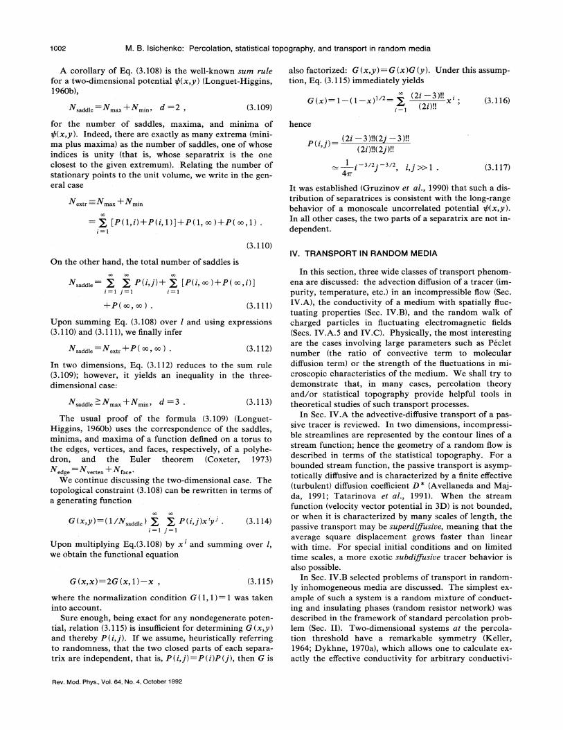
1002 M. B. lsichenko: Percolation, statistical topography, and transport in random media
A corollary of Eq. (3.108) is the well-known sum rulefor a two-dimensional potential g(x,y) (Longuet-Higgins,1960b),
saddle max ++min ~ (3.109)
+extr =+max ++min
[P( l, i)+P(i, 1)]+P(1,oo )+P( oo, 1) .i=1
for the number of saddles, maxima, and minima ofg(x,y). Indeed, there are exactly as many extrema (mini-ma plus maxima) as the number of saddles, one of whoseindices is unity (that is, whose separatrix is the oneclosest to the given extremum). Relating the number ofstationary points to the unit volume, we write in the gen-eral case
( 2i —3 )!!6(x)=1—(1—x)' = g "x';(2i)!!
(3.116)
hence
(2i —3)!!(2j—3)!!( 2i )!!(2j )tt
~ —3/2 ~ —3/2j i,j»1 . (3.117)
It was established (Cxruzinov et al. , 1990) that such a dis-tribution of separatrices is consistent with the long-rangebehavior of a monoscale uncorrelated potential f(x,y).In all other cases, the two parts of a separatrix are not in-dependent.
also factorized: 6 (x,y) =6(x)6 (y). Under this assump-tion, Eq. (3.115) immediately yields
On the other hand, the total number of saddles is
(3.110)IV. TRANSPORT IN RANDOM MEDIA
N„dd), = g g P(i j)+ g [P(i, oo)+P(oo, i)]I=l J=l i=1
+P(oo, o)o. (3.111)
Upon summing Eq. (3.108) over l and using expressions(3.110) and (3.111),we finally infer
N ddi =N +P( ) (3.112)
In two dimensions, Eq. (3.112) reduces to the sum rule(3.109); however, it yields an inequality in the three-dimensional case:
+saddle —fornax +Km;II, d =3 (3.113)
The usual proof of the formula (3.109) (Longuet-Higgins, 1960b) uses the correspondence of the saddles,minima, and maxima of a function defined on a torus tothe edges, vertices, and faces, respectively, of a polyhe-dron, and the Euler theorem (Coxeter, 1973)+edge +vertex ++face '
We continue discussing the two-dimensional case. Thetopological constraint (3.108) can be rewritten in terms ofa generating function
6(x,y)=(1/N„~d„) g g P(i, j)x'y' .i =l j=l
(3.114)
Upon multiplying Eq.(3.108) by x and summing over i,we obtain the functional equation
6(x,x)=2G(x, 1)—x, (3.115)
where the normalization condition G (1,1)=1 was takeninto account.
Sure enough, being exact for any nondegenerate poten-tial, relation (3.115) is insufficient for determining 6 (x,y)and thereby P(i,j). If we assume, heuristically referringto randomness, that the two closed parts of each separa-trix are independent, that is, P(ij )=P(i)P(j), then 6 is
In this section, three wide classes of transport phenom-ena are discussed: the advection diffusion of a tracer (im-
purity, temperature, etc.) in an incompressible fiow (Sec.IV.A), the conductivity of a medium with spatially fiuc-tuating properties (Sec. IV.B), and the random walk ofcharged particles in fluctuating electromagnetic fields(Secs. IV.A.5 and IV.C). Physically, the most interestingare the cases involving large parameters such as Pecletnumber (the ratio of convective term to moleculardiffusion term) or the strength of the fiuctuations in mi-
croscopic characteristics of the medium. We shall try todemonstrate that, in many cases, percolation theoryand/or statistical topography provide helpful tools intheoretical studies of such transport processes.
In Sec. IV.A the advective-diffusive transport of a pas-sive tracer is reviewed. In two dimensions, incompressi-ble streamlines are represented by the contour lines of astream function; hence the geometry of a random Bow isdescribed in terms of the statistical topography. For abounded stream function, the passive transport is asymp-totically diffusive and is characterized by a finite effective(turbulent) diffusion coefficient D* (Avellaneda and Maj-da, 1991; Tatarinova et al. , 1991). When the streamfunction (velocity vector potential in 3D) is not bounded,or when it is characterized by many scales of length, thepassive transport may be superdi+usiue, meaning that theaverage square displacement grows faster than linearwith time. For special initial conditions and on limitedtime scales, a more exotic subdiQusiue tracer behavior isalso possible.
In Sec. IV.B selected problems of transport in random-ly inhomogeneous media are discussed. The simplest ex-ample of such a system is a random mixture of conduct-ing and insulating phases (random resistor network) wasdescribed in the framework of standard percolation prob-lem (Sec. II). Two-dimensional systems at the percola-tion threshold have a remarkable symmetry (Keller,1964; Dykhne, 1970a), which allows one to calculate ex-actly the effective conductivity for arbitrary conductivi-
Rev. Mod. Phys. , Voj. 64, No. 4, October 1992

M. B. Isichenko: Percolation, statistical topography, and transport in random media 1003
ties of the two phases. Other examples include plasmaheat conduction in a stochastic magnetic Geld and theelectrical conductivity of randomly inhomogeneousmedia with the Hall effect.
In Sec. IV.C the multifaceted aspects of electronmotion in disordered potentials are discussed in the ex-amples of a few models. Special attention is given to theiong-range correlation effects that the magnetic field in-troduces into the processes of electron scattering bydisordered potentials.
A. Advective-diffusive transport
Everyone will acknowledge the striking effect the stir-ring of a teaspoon exerts on the sugar dissolution in a cupof coffee. A vast variety of processes, ranging fromeveryday propagation of smell to heat transport in fusionplasma, can be cast into the simplest form of theadvection-difFusion equation
n +V [nv(x, t)]=DOV n,Bt
(4.1)
where n is the density of a passively advected agent (con-centration of an impurity, temperature, etc.), v is a veloc-ity field, and Do is the molecular difFusion coefficient orthermal conductivity. In most practically applicablecases, velocity v(x, t) can be considered to be incompres-sible: V v=0, or v=VXQ(x, t), where g is a vector po-tential. Along with Eq. (4.1), the problem can beequivalently formulated in terms of a random trajectoryof tracer particle described by the Langevin equation(Chandrasekhar, 1943)
dx =v(x, t)+ vD(t),dt
(4.2)
where vD(t) is a Cxaussian random noise corresponding tothe molecular diffusion, so that
(vD(t)) =0, (UD;(t)UD~(t')) =2DO&(t —t')&;J . (4.3)
((x;(t)—x;(0))(x (t) —x (0)))lim J J D )fc
g~ oo 2t EJ(4.4)
where D,*. is the efFective, or turbulent, diffusivity tensor.Taylor (1921) related the effective diffusivity to the La-grangian velocity correlator
Then the probability distribution function n (x, t) of theparticle position x evolves according to the Fokker-Planck equation (4.1).
In 1921, G. Taylor put forward the hypothesis of"difFusion by continuous movements. " According to thishypothesis, the solution of Eq. (4.2) for a turbulent, zeromean velocity field v(x, t) behaves diffusively in the long-time limit, so that
This well-known result, however, is almost a tautology,because in order to obtain V; (t) one has first to solve theequation of motion (4.2). The Taylor hypothesis of theturbulent difFusion behavior corresponds to a decay ofLagrangian correlations sufticiently fast so that integral(4.5) converges.
Richardson (1926) analyzed then-available experimen-tal data on diffusion in air. Those data varied by 12 or-ders of magnitude, indicating that there is somethingwrong with the Taylor hypothesis. Richardson phenom-enologically conjectured that the diffusion coefficient D&in turbulent air depended on the scale length k of themeasurement. The Richardson law,
(4.6)
was related to the Kolmogorov-Obukhov turbulencespectrum, Uz ~ A'~, by Batchelor (1952). So the effectivediffusion limit (4.4) does not necessarily exist. It must beemphasized that the Richardson law (4.6) describes therelatiue diQusiuity of suspended particles, that is, the rateof growth of the mean-square distance between two fluidelements in the turbulent medium. The absolute diji"usionin Kolmogorov turbulence is not universal because theboundary-condition-dependent long-scale velocity pulsa-tions govern the absolute motion of a fluid element andmay make the integral (4.5) diverge (Moffatt, 1981).
There exists, however, an important class of in-compressible flows that do lead to a finite absolute tur-bulent diff'usion coefficient (4.4), namely, the fiows with abounded velocity vector potential P(x, t) In Sec. I. V.A. 1
recent rigorous results are reviewed concerning suchflows. In Sec. IV.A.2 certain regular flows are listed forwhich the effective difFusivity D* is known exactly or canbe easily estimated in order of magnitude. SectionIV.A.3 is devoted to the problem of turbulent diffusion inrandom, steady 2D flows, which are described usingpercolation/statistical topography theory. In Sec.IV.A.4 chaotic mixing properties of unsteady randomflows are studied and characterized by Kolmogorov en-
tropy. Effective diffusion in such flows is discussed inSec. IV.A.5. The applications of the theory of transportby time-dependent random flows are primarily concernedwith and exemplified by the anomalous transport in tur-bulent plasmas.
Even when the effective diffusivity D* governs theasymptotic tracer behavior in an advection-diffusion sys-tem, this behavior has finite set-in (mixing) time andlength scales. On time and space scales below the mixingtime r and the mixing scale g, passive scalar transportcan be anomalous, meaning that the propagation rate isdescribed by
V,,(t) = (U, (x(t), t)U, (x(0),0) ) ([x(t)—x(0)] )'~ t~, (4.7)
as follows:
D,'= I V,"(t)dt . (4.5)with gA —,
' instead of the behavior of Eq. (4.4). For fiows
with unbounded vector potential @(x) the mixing time
Rev. Mod. Phys. , Vol. 64, No. 4, October 1992

1004 M. B. Isichenko: Percolation, statistical topography, and transport in random media
may be infinite, with the anomalous diffusion (4.7)featuring the long-time behavior. The mechanisms ofanomalous difFusion, including both superdiffusion ( g ) —, )
and subdi+usion (g & —,' ), are discussed in Sec. IV.6.A. (&r « t (4.13)
(x, r) over such length scales g and time scales r thatsatisfy
1. When is the effective transport diffusive,and what are the bounds on effective diffusivity?
0P=0
(4.9)
known as the Peclet number, where $0 is some charac-teristic (for example, root-mean-square) value of the vec-tor potential tP(x, t). According to the Zeldovich varia-tional principle, efFective diffusivity, if it exists, must ex-pand in a series of even powers of the Peclet number:
D*=DO(1+a2P +a4P + ), P ((1, (4.10)
where az & 0. In the limit of a large Peclet number, it isnatural to expect that the efFective diffusivity greatlyexceeds the molecular one:
D'=D0P, P»1,where the non-negative exponent cx depends on the topol-ogy of the Aow.
A more dificult question concerns the very realizabili-ty of the effective diffusion regime and the upper boundsfor effective diffusivity. Strictly speaking, condition (4.4)does not yet imply the efFective diffusion of a tracer. Astronger requirement is that the local-average tracer den-sity (n ) evolve according to the effective difFusion equa-tion
B(n )at
B,B(n)lJ (4.12)
The local average of the density n is taken near the point
This question has been posed frequently, first by Zeldo-vich (1937), who showed that the lower bound for theeffective diffusivity D is simply the molecular diffusivityD0. To be more exact, his result was that arbitrary in-compressible convection in a Quid necessarily increases(with respect to the absence of convection) the averageimpurity Aux J between two surfaces where the two con-stant impurity densities, n
&and n2, are maintained. The
idea of the proof is based on a simple variational princi-ple: Integrate the quantity (nv DoVn—).Vn over thevolume outside the two closed surfaces. Then the resultis
J(n, n2)—=Do J(Vn) dx .
The right-hand side of Eq. (4.8) is minimized by a har-monic function, V n =0, which corresponds to the zerovelocity field in the time-independent (or time-averaged)Eq. (4.1).
Effective transport in a convection-diffusion system isgoverned by the dimensionless parameter
where g and r are the flow-dependent mixing length
and mixing time, respectively, and l and t* are thecharacteristic length and time scales of ( n ). As inequal-ities (4.13) show, the set-in of effective diffusion takesfinite mixing time r; hence Eq. (4.12) becomes valid
only asymptotically.Another approach to the effective diffusion problem is
to consider the velocity field v(x, t) as a stationary ran-dom field and to average the tracer density n over the sta-tistical ensemble of v. Pioneered by Taylor (1921), thisapproach remains the most popular (Kraichnan, 1970;McLaughlin et al. , 1985; Avellaneda and Majda, 1989,1991). Kraichnan (1970) undertook the explicit compu-tation of the mean-square particle displacement in 2Dand 3D Gaussian velocity fields, averaging over 2000realizations for each ensemble. There was no moleculardiffusion in this simulation, and both time-dependent and"frozen" velocity fields were tested. In each case, exceptfor the case of two-dimensional time-independent Aows,Kraichnan observed a well-established turbulentdiffusivity (4.4).
Another computational approach, proposed by Isi-chenko et al. (1989), used a prescribed quasiperiodicstream function g(x,y) (such as the one shown in Fig. 10)as a model of random How. Although not random, theHow has no apparent degeneracies, such as periodicity,and looks quite generic. However, one still can visuallyidentify a "trace of periodicity, " especially for a smallnumber X of harmonics, because the Aow pattern is atwo-dimensional projection of an X-dimensional periodicstructure. (In Fig. 10, the case of N =25 isshown. ) In addition, the space-averaged correlatorC(p) = (g(x)f(x+p) )„does not vanish at large scales,showing long correlations that are characteristic forquasicrystals (Levine and Steinhardt, 1984; Kaluginet al. , 1985; Steinhardt and Ostlund, 1987; Arnold,1988). These correlations were not found to affect appre-ciably the advective-diffusive transport in steady Qows forN) 3 (Isichenko et al. , 1989). Yet, the quasicrystalliccorrelations appear to be much more pronounced fordifFusion in time-dependent 2D flows (see Sec. IV.A.5).
Analytical results regarding the criterion of the transi-tion to effective diffusion were obtained by McLaughlinet al. (1985), who proved the following homogenization
property of time-independent, incompressible, zero mean,stationary random flow v(x). If the Fourier transformV;.(k) of the velocity correlator VJ(p)=(U;(x)v~(x+p))is continuous at the origin k=0, then the ensemble-averaged solution of Eq. (4.1), ( n ) =N, (x, t), corre-sponding to the initial condition n(x, O)=no(cx), be-comes very close, as E~O, to N(x/e, t/E ), where N(x, t)is the solution of the initial-value problem
Rev. Mod. Phys. , Vol. 64, No. 4, October 1992

M. B. lsichenko: Percolation, statistical topography, and transport in random media 1005
BX 8 ~ BNBt Bx; J Bxz
X(x,O) =no(x),(4.14)
and effective diffusivity in any direction n exceeds molec-ular diffusivity:
D*(n)=—)n~ D;*n, n ~Do . (4.15)
Battacharya et al. (1989) obtained a similar result forarbitrary periodic incompressible Qow, without ensembleaveraging. Kalugin et al. (1990) proved a homogeniza-tion theorem for periodic Aows using the analytical con-tinuation of D,*(P), con.sidered as a function of the Pecletnumber P =g, ,/Do, to the complex plane of P Such. anapproach led to an eKcient algorithm for the computa-tion of D; for any periodic Aow using continuous frac-tions.
Avellaneda and Majda (1989, 1991) generalized theMcLaughlin et al. (1985) result and showed that thefiniteness of the Peclet number {4.9) {with $0 understoodas the ensemble root-mean-square vector potential) is anecessary and sufficient condition to guarantee the homo-genization property for time-independent random Aowsv(x)=VX/(x). They also developed a theory of Padeapproximants using a Stieltjes measure representationformula for effective diffusivity. This theory led to a se-quence of rigorous bounds on D, of which the simplestone is
Thus one may conclude that, in the presence of finitemolecular difFusivity Do, the finite vector potential is asufficient and "almost necessary" condition for effectivediffusion to be established, with efFective diffusivity satis-fying the inequality
2.
Do ~D* ~DO+Do
(4.19)
In terms of the scaling exponent a entering Eq. (4.11),this implies 0 ~ o. ~ 2.
For the case of anisotropic molecular diffusivity tensorBo and a possible anisotropy of the How, following thelines of Tatarinova et al. (1991), inequality (4.19) can begeneralized to
DO„~D„' ~DO„+max max[mXn f(x, t)]
Dom(4.20)
2. Effective diffusivity: Simple scalings
where D„:D; n,—n /~n~ denotes the diffusivity in the ndirection. It is clear that inequality (4.19) is a conse-quence of (4.20). Result (4.20) will be used in Sec. IV.B.3to establish bounds on the effective conductivity ofheterogeneous media. %'ithout restricting the class ofthe vector potential g, inequalities (4.19) and (4.20) can-not be further improved in the sense that both the lowerand the upper bounds on the effective diffusivity can berealized in particular cases.
(4.16)
where d is the dimension of the problem. Generally, thefirst two terms in the low-P expansion (4.10) turn out tobe an upper bound for D* at any P.
Independently, Tatarinova et al (1991) con. sidered themost general case of an arbitrary incompressible 3Dtime-dependent fIow. They gave an elegant proof of thefollowing theorem: If the vector potential 1lI(x, t) of agiven Bow is bounded, ~f(x, t)
~
~ g,„, then the solutionof the initial-value problem (4.1) with n (x,O) =5(x—xo)behaves as follows. The mean-square displacement,
R (t, xo)= J(x—xo) n(x, t)dx, (4.17)
grows with progressing time not slower and not fasterthan linearly in the sense that
&~'(t, x, ))„Do ~ ~DO+ (4.18)
2td— ' D,
Most likely, the averaging of R over the initial positionxo is not essential for this result. The comparison of theTatarinova et al. theorem with the Avellaneda-Majdatheorem suggests that the boundedness of the vector po-tential f(x, t) is also sufficient for the global transporthomogenization, that is, for the asymptotic transitionfrom Eq. (4.1) to Eq. (4.12). In such a general form, how-ever, the homogenization theorem has not yet beenproved.
a 2v 2
D*=DO+XDo
(4.21)
with different values of the numerical constant K. Fur-ther generalizations are reviewed by Young and Jones(1991).
Zeldovich (1982) considered the periodic time-dependent How in the (x,y) plane,
v= vox cosky cosset,
and found the effective difFusivity in the x direction:
(4.22)
There exist several classes of Aows, whose transportproperties can be calculated exactly. As we shall see, therigorous bounds on the effective diffusivity (4.19) are at-tainable.
The simplest example of a shear Row in a tube wasconsidered by Taylor (1953, 1954), who noticed that theaxial dispersion of a solute advected by the PoiseuilleHow u (r) =uo(1 r /a ) [where u (—r) is the axial velocityin a tube of the radius a] is described, in a mean velocityframe of reference, by a diffusive law. For avo))Do,Taylor found the following equation for the "virtualcoefficient of the diffusivity": D*=a uii/(192DO). Heproposed to use this result for the investigation of thepropagation of salts in bloodstreams. Aris (1956) hasgeneralized Taylor's result to the case of arbitrary Pecletnumber P =avo/Do and different tube cross sections,where all possibilities are covered by one exact formula,
Rev. Mod. Phys. , VoI. 64, No. 4, October 1992

1006 M. B. lsichenko: Percolation, statistical topography, and transport in random media
k UpD D0 1 +
2 4 pr
2 ~+a +0(4.23)
In the case of a general time-independent shear flowv=xdg(y)/dy, (f(y))»=0, one has (Avellaneda andMajda, 1990; Isichenko and Kalda, 1991a) D* =Do,
( '(y)&,D*„=Do+0
(4.24)
The above results are obtained by separating the tracerdensity n into an oscillating and a smoothed component,a method similar to the technique of multiple-scale ex-pansion (cf. Bender and Orszag, 1978). The physicalmeaning of result (4.24) is quite simple: Due to themolecular diffusion in the y direction, a tracer particle re-sides in a channel with the same direction of velocity fora characteristic correlation time ~ =A,p/Dp, where kp isthe characteristic scale of the flow. The advective dis-placement experienced by the particle during this time is
g~ =uor . The effective diffusivity in the x direction isthen estimated as D *=g /r =A, ou o /Do, in accordancewith (4.24). Quantities g and r represent the mixinglength in the x direction and the mixing time, respective-ly.
In terms of the scaling exponent a [see Eq. (4.11)], theresult (4.24) corresponds to the maximum possible valuea=2. This is quite sensible because open (e.g., straight)streamlines promote the best imaginable mixing alongtheir direction, the exact straightness of streamlines be-ing not necessary for the a =2 scaling to hold (Childressand Soward, 1989; Crisanti et al. , 1990). By the way, theexact maximum of D*, given by Eq. (4.19), is also at-tained by a shear flow with a steplike stream function
g(y) =11osgnf (y), (f(y) )» =0, (4.25)
corresponding to vanishingly narrow velocity jets locatedat the zero lines off (y). According to formula (4.24), we1 ave D,*„=Do+to/Do =Do+0'-/Do
The second class of flow with a simple effectivediffusion scaling is a periodic array of convection rolls,such as those modeled by the stream function
P(x,y) =gosink„x sink»y (4.26)
D*=C t/ Dogo, I':Qo/Do )) 1 . — (4.27)
It was later in 1987 that flow (4.22) drew much attention(Osipenko et al. , 1987; Perkins and Zweibel, 1987;Rosenbluth et al. , 1987; Shraiman, 1987; Soward, 1987).Using an asymptotic expansion for periodic fields (Ben-soussan et al. , 1978; Brenner, 1980) or methods similar inspirit, the problem was reduced to the effectively one-dimensional cross-stream diffusion within one convectioncell, making it possible to calculate the numerical con-
(see Fig. 20). For this, topologically similar flows, and itssimplest generalizations, it was noticed (Dykhne, 1981;Moffatt, 1983) that the large-Peclet-number asymptoticsof D* correspond to the exponent a =
—,':
FIG. 20. Periodic system of convection rolls described by thestream function (4.26). The hatched region denotes di6'usiveboundary layers near the separatrices, where the tracer densitygradients are localized in the high-Peclet-number limit.
stant C in Eq. (4.27). Formula (4.27) was confirmed in aspecially designed experiment (Solomon and Gollub,1988), where passive tracer transport was studied in aperiodic system of controlled Rayleigh-Benard convec-tion rolls.
The +Do scaling is due to the formation, in thelarge-Peclet-number limit, of diffusive boundary layersnear the separatrices (Fig. 20), where the tracer densitygradients turn out to be concentrated. Being of majorsignificance for effective transport, the boundary layerwidth wb is determined as the characteristic diffusive dis-placement a tracer particle undergoes in the course of theadvective rotation period:
wb ="(/Do~o/uo ~ (4.28)
where A,o is the cell size and uo =go/A, o is the characteris-tic velocity. Then the effective diffusivity is estimated interms of the usual random-walk expression A,o/(ko/uo)multiplied by the fraction of "active" particles wb/Xp ly-ing in the boundary layer. This leads to the result
)fcD —Up Wb (4.29)
revealing scaling (4.27).It is interesting to note that, while the periodic flow
(4.26) was generally invoked to model steady Rayleigh-Benard convection (Chandrasekhar, 1961; Haken, 1977;Busse, 1978), the effective diffusivity in the Rayleigh-Benard system may behave quite differently from the pre-diction of formula (4.27) (Dykhne, 1981). There are twoprinciple patterns of steady convection in a fluid heatedfrom below, namely, rolls [Fig. 21(a)] and hexagons [Fig.21(b); Busse, 1978]. The transport properties of rolls areproperly modeled by flow (4.26) for the case of "free-slip"boundaries at the bottom of the vessel. In the case of"no-slip" boundary condition, the effective diffusivity D *
scales proportional to Do (Rosenbluth et al. , 1987).Unlike the roll convection pattern, the separatrices ofRayleigh-Benard hexagons include not only the inter-faces between the cells but also the cells' axes [Fig. 21(b)].
Rev. Mod. Phys. , Vol. 64, No. 4, October 1992
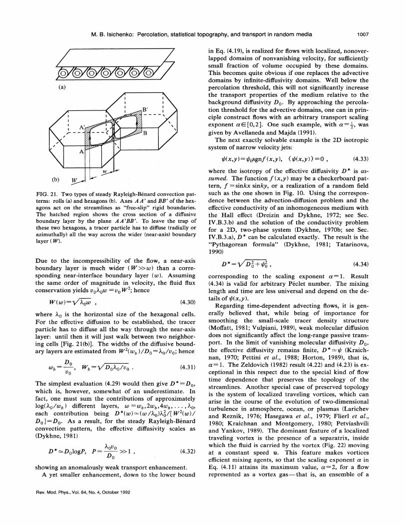
M. B. Isichenko: Percolation, statistical topography, and transport in random media 1007
(a)
A'
A
in Eq. (4.19), is realized for flows with localized, nonover-lapped domains of nonvanishing velocity, for sufticientlysmall fraction of volume occupied by these domains.This becomes quite obvious if one replaces the advectivedomains by infinite-diffusivity domains. Well below thepercolation threshold, this will not significantly increasethe transport properties of the medium relative to thebackground diffusivity Dp. By approaching the percola-tion threshold for the advective domains, one can in prin-ciple construct Aows with an arbitrary transport scalingexponent a&[0,2]. One such example, with a= —,', was
given by Avellaneda and Majda (1991).The next exactly solvable example is the 2D isotropic
system of narrow velocity jets:
f(x,y) =gosgnf (x,y), (g(x,y) ) =0, (4.33)
(b) ~W
FIG. 21. Two types of steady Rayleigh-Benard convection pat-terns: rolls (a) and hexagons (b). Axes A A ' and 88' of the hex-agons act on the streamlines as "free-slip" rigid boundaries.The hatched region shows the cross section of a diffusiveboundary layer by the plane AA'88'. To leave the trap ofthese two hexagons, a tracer particle has to diffuse (radially orazimuthally) all the way across the wider (near-axis) boundarylayer ( 8').
Due to the incompressibility of the Bow, a near-axisboundary layer is much wider (W))tv) than a corre-sponding near-interface boundary layer (tv). Assumingthe same order of magriitude in velocity, the Quid Aux
conservation yields vpkpw =Up 8 ' hence
W(w) =+Row (4.30)
Do
VpSb +Do~o/vo . (4.31)
The simplest evaluation (4.29) would then give D*=Do,which is, however, somewhat of an underestimate. Infact, one must sum the contributions of approximatelylog(Ao/tvb ) different layers, w =wb, 2wb, 4mb, . . . , Ao,
each contribution being D *(w) = ( tv /go)A~~/[ W2( w ) /Do]=Do. As a result, for the steady Rayleigh-Benardconvection pattern, the effective diffusivity scales as(Dykhne, 1981)
A,pUpD =DplogP, P = ))1,
p(4.32)
showing an anomalously weak transport enhancement.A yet smaller enhancement, down to the lower bound
where A,p is the horizontal size of the hexagonal cells.For the effective diffusion to be established, the tracerparticle has to diffuse all the way through the near-axislayer: until then it will just walk between two neighbor-ing cells [Fig. 21(b)]. The widths of the diffusive bound-ary layers are estimated from 8' (tv& )/Do =A,o/vo; hence
where the isotropy of the effective diffusivity D is as-sumed. The function f (x,y) may be a checkerboard pat-tern, f =sinkx sinky, or a realization of a random fieldsuch as the one shown in Fig. 10. Using the correspon-dence between the advection-diffusion problem and theeffective conductivity of an inhomogeneous medium withthe Hall effect (Dreizin and Dykhne, 1972; see Sec.IV.B.3.b) and the solution of the conductivity problemfor a 2D, two-phase system (Dykhne, 1970b; see Sec.IV.B.3.a), D' can be calculated exactly. The result is the"Pythagorean formula" (Dykhne, 1981; Tatarinova,1990)
D e QD2+y2 (4.34)
corresponding to the scaling exponent a = 1. Result(4.34) is valid for arbitrary Peclet number. The mixinglength and time are less universal and depend on the de-tails of g(x, y).
Regarding time-dependent advecting Bows, it is gen-erally believed that, while being of importance forsmoothing the small-scale tracer density structure(Moffatt, 1981; Vulpiani, 1989), weak molecular diffusiondoes not significantly affect the long-range passive trans-port. In the limit of vanishing molecular diffusivity Dp,the effective diffusivity remains finite, D*=P (Kraich-nan, 1970; Pettini et al. , 1988; Horton, 1989), that is,a= l. The Zeldovich (1982) result (4.22) and (4.23) is ex-ceptional in this respect due to the special kind of Howtime dependence that preserves the topology of thestreamlines. Another special case of preserved topologyis the system of localized traveling vortices, which canarise in the course of the evolution of two-dimensionalturbulence in atmosphere, ocean, or plasmas (Larichevand Reznik, 1976; Hasegawa et al. , 1979; Flierl et al. ,1980; Kraichnan and Montgomery, 1980; Petviashviliand Yankov, 1989). The dominant feature of a localizedtraveling vortex is the presence of a separatrix, insidewhich the fluid is carried by the vortex (Fig. 22) movingat a constant speed u. This feature makes vorticesefficient mixing agents, so that the scaling exponent cz inEq. (4.11) attains its maximum value, a=2, for a flowrepresented as a vortex gas —that is, an ensemble of a
Rev. Mod. Phys. , Vol. 64, No. 4, October 1992

1008 M. B. Isichenko: Percolation, statistical topography, and transport in random media
FICi. 22. Typical pattern of streamlines in a traveling dipolevortex, shown in the frame of reference moving together withthe vortex. The hatched region surrounded by a separatrix(heavy line) represents the trapped Quid transported by the vor-tex.
large number of traveling vortices —whose interactionsare unessential. The effective diffusivity of the vortex gasfor the large-Peclet-number limit was calculated by Isi-chenko et al. (1989):
D,*=rj(sr u;u )+DO5,/, (4.35)
where g is the number of vortices per unit area, s =A,0 isthe area enclosed by the separatrix of a vortex,
=A,o/Do is a diff'usion time inside the vortex, and theaveraging in (4.35) is taken over the vortices. The esti-mate of the exact result (4.35) can be obtained as follows.A tracer particle is trapped and carried by a vortex forthe diffusion time r =A,o/Do and then released the dis-
tance g =ur away from the point of trapping. Theeff'ective diffusivity is then obtained as g /r multiplied
by the fraction of area, gA, ~, where the trapping processestake place. The resulting expression, D*=qk0u /D0,agrees with formula (4.35) for sufficiently high Pecletnumber, I' =A,ou /Do &)(r)A,O)
' )&1. The effects ofvortex collisions (Horton, 1989) and of the inhomogenei-
ty of the vortex-supporting medium (Zabusky andMcWilliams, 1982; Nycander and Isichenko, 1990) leadto various regimes of effective diffusion, including thosefor which the molecular diffusivity D0 is unessential. Ad-vective transport by time-dependent random Aows is dis-cussed in Sec. IV.A.5.
3. Diffusion in two-dimensional random,steady flows
As we have seen, the behavior of effective diffusivity inthe large-Peclet-number limit depends on the topology ofNow streamlines. The best Inixing properties are exhibit-ed by Aows with extended streamlines, such as shearfiows, where the mixing length g' tends to infinity asD0~0. The geometry of 2D random Aows assumes the
where the exponent was expressed through the 2D per-colation indices v= —', and d& =—', .
Vdh+1
vdg +21013
' (4.37)
Due to the role of extended streamlines of a random How,the effective diffusivity (4.36) greatly exceeds Eq. (4.27),valid for finite-size convection cells, at the same largePeclet number.
The derivation of result (4.36) employs a hypothesis ofbroken coherence. This hypothesis assumes that the par-ticle displacements governed by Eq. (4.2) may be con-sidered to be uncorrelated if the streamlines on whichthese displacements are experienced differ twice or morein size. In this way, one comes naturally to the conceptof convection cells being the conglomerates of stream-
presence of arbitrarily large streamlines, although theirshare falls with the increasing size. To estimate theeffective diffusivity in such a How, statistical topographymust be used for the description of the streamlines (Isi-chenko et al. , 1989; Gruzinov et al. , 1990; Isichenko andKalda, 1991c).
It is dificult to imagine a time-independent or a slowlytime-dependent 2D random Aow in such traditional 2Dhydrodynamic objects as atmosphere and ocean wherethe characteristic frequency co is typically of the order ofthe inverse eddy rotation time, co= uo/Ao. The practicalimplications of "frozen, " or "quenched" 2D randomAows involve primarily condensed-matter objects, such asquantum diffusion (Kravtsov et al. , 1986), the quantumHall eff'ect (Prange and Girvin, 1990), or inhomogeneous-ly doped semiconductors (Dreizin and Dykhne, 1972; Isi-chenko and Kalda, 1991a).
The erst percolation theory analysis of effectivediffusion in a 2D, random, incompressible, steady How(Isichenko et al. , 1989) was motivated by the observationthat the periodic Qow pattern (4.26) is structurally unsta-ble: A vanishingly small perturbation of the stream func-tion will destroy the regular system of elementary con-vective cells, gather them into various conglomerates,and thereby produce arbitrary length scales in the iso-lines of g(x,y) (see Fig. 11). Although there is no doubtabout the existence of a well-de6ned effective diffusivityD* for a bounded random stream function f(x,y), therehas been developed no formal theory leading to therigorous calculation of D for a large Peclet number.The small-Peclet-number expansion for random Aowswas developed by Derrida and Luck (1983), Fisher(1984), Kravtsov et al. (1986), and Bouchaud et al.(1987) using path integrals and the renormalization-group theory.
For a monoscale stream function P(x,y) (Fig. 10)heuristic arguments were used (Isichenko et al. , 1989) toderive the 0.= —,", scaling
10/13
D (4.36)0
Rev. Mod. Phys. , Voa. 64, No. 4, October 1992

M. B. Isichenko: Percolation, statistical topography, and transport in random media 1009
L(g ) tv (g )
Up Dpwhere vo =go/A, o is the characteristic velocity. Substitut-ing Eqs. (3.43) and (3.45) for the length L (a) and thewidth w(a) of the convection cell, we find
(4.38)
(4.39)
The effective diffusivity is then estimated to be
D*=F(g ) 2 =votv(g ),$2
tv (g )/Do(4.40)
where F(a)=L(a)w(a)/a is the distribution function(area fraction) of the convection cells over their size.Upon substituting Eq. (4.39) into (4.40), we arrive at theresult (4.36). The mixing time in a monoscale Ao flow isgiven by the formula
lines with diameter between a and 2a ("a cells"; see Fig.17). The mixing length g is then determined as the sizeof convection cells producing the most efficient coherentcontribution to transport. The calculation is quite simi-lar to that based on the boundary-layer argument for aperiodic array of vortices (Fig. 20). The difference, how-ever, is that the convection cells of a random Row arediverse, and their size a, width w (a), and perimeter L (a)are coupled in a fashion determined by the statistics ofthe random field f(x,y). For example, for a monoscale(A,o) flow, the relations given by Eqs. (3.43) and (3.45)should be used. Using the standard boundary-layer argu-ment, we find the mixing length g to be the cell sizewhere the convection time equals the transverse diffusiontime,
D*=f, D. "'0
(4.43)
logA Po
dh +1/vThe partial diffusivity D& ~A, " increases with in-creasing scale A., making expression (4.43) peak near theupper integration limit.
The percolation scaling of effective diffusivity involv-ing the exponent o.= —,", appears to be as universal as thestatic exponents of continuum percolation (see Sec. II.E).This implies that the randomness (in the sense of the en-semble averaging) of the velocity field is not really neces-sary for the result (4.36) to be valid; the genericity (i.e.,the absence of exceptional features like periodicity, etc.)
of the Qow will sufFice. The computation of effectivediffusion for quasiperiodic Aows having extended stream-lines showed a fair agreement with the —,", scaling (Isi-chenko et al. , 1989).
A similar approach was used to calculate the effectivediffusivity in a multiscale random How with the streamfunction spectrum gi ~X, Ac&A, &A, (Isichenko andKalda, 1991c). Due to a more sophisticated dependenceof L(a) and w(a) [see Eqs. (3.74), (3.78), and (3.80)],there are several regimes of effective diffusion in thisHow. The regimes are depicted in Fig. 23, where the pa-rameter space (H, log& /n (A, /Ao)) is shown. One of
0 0
these regimes, corresponding to the monoscale correlated
Xpm
p(4.41)
(0) (m)
corresponding to the time of diffusive sampling of all"undermixing" (that is, with a & g ) convection cells.
Equation (4.40) describes the efFective diffusion contri-bution of mixing (g ) convection cells only. Neverthe-less, this contribution constitutes of order one-half theeffective diffusivity, thereby yielding a correct estimate ofD*. The contribution of more numerous undermixingcells with A, & g can be written similarly to (4.40):
34
1017
(4.42)
The hypothesis of broken coherence implies that effectivediffusivity can be estimated as the sum of partialdiQusi vities D i, for A, = A,o, 2i,o, 4i,o, . . . , g, that is,
The contribution of "overmixing" convection cells with di-ameter A, »g is negligible due to both the scarcity of suchcells and the di8'usive decorrelation that occurs well before par-ticles sample their extent.
FICx. 23. Regimes of eft'ective di6'usion in a multiscale, steady,random 2D How (Isichenko and Kalda, 1991c)shown in the pa-rameter space (H, logPO /logA), where Po = fq /Do is the
short-scale Peclet number and A=A, /A. o is the width of theflow spectrum. Expression D*= i(OPO A for effective diffusivityincludes the following exponents in regimes (A —D): (A)a= —1/(vdg+2), y=(vHdp, +DI, )/(vdp+2); (B) a=H/(Dp—2H), y=O; (C) a=O, y=H; (D) o.=(2—D&/H)/(vd&+2),y=(vHdh+Dz )/(vdI, +2). Regimes (0) and (m) correspond todiffusion in the monoscale flows t/iz (x) and g~ (x), respective-
0 m
ly. In the hatched region, D* is of the order of Do.
Rev. Mod. Phys. , Vol. 64, No. 4, October 1992

1010 M. B. Isichenko: Percolation, statistical topography, and transport in random media
stream function (regime B in Fig. 23), is recovered bysimple replacement of the random percolation exponentsby their correlated counterparts (see Sec. II.D),
1 1v~ ——,d —+D, ——&H &0 .h h~ (4.44)
In this case we have from Eq. (4.37)
Dh—/H+IDq—/H +2
10(1 H)— 3——&H&0.10—17H ' 4
(4.45)
For H tending to zero, a tends to unity and the effectivediffusivity D * becomes independent of Do. Such in-dependence extends to regime C. Regime 3, which ischaracterized by the monoscalelike scaling D ' ~ D o ', isobtained by substituting the partial diffusivity Dz (4.42)
m
into the monoscale flow gi (x,y) and using formula
(4.36). In this representation, D& is the renormalizedm
molecular difFusivity, which accounts for the transporteffect of the How spectral components with A, & A,
4. Lagrangian chaos and Kolmogorov entropy
Thus far we have been concerned with "frozen" Aows,or systems with "unessential" time dependence thatpreserves the topology of streamlines, that is, where thetracer orbits would be regular in the absence of themicrodiffusivity. In the case of an "essential" timedependence in two dimensions, where the topology ischanged, or in three dimensions even without timedependence, the orbits are generally chaotic, leading to adiffusionlike random walk.
The general reason for the decay of orbit correlationsin (4.5), and hence for the transition to the effectivedifFusion or other kinds of random walk, is found inHamiltonian chaos (Chirikov, 1979; Lichtenberg andLieberman, 1983; Sagdeev et al. , 1988). Consider a two-dimensional How with Do=0. Then the equations ofmotion of a fIuid element,
dx Bg(x,y, t) dy Bg(x,y, t)dt By dt Bx
(4.46)
correspond to the Hamiltonian g defined in the phasespace (x,y). The Liouville theorem is equivalent to theincompressibility of the flow v =VQXz. The one-degree-of-freedom time-dependent Hamiltonian P(x,y, t)is equivalent to a two-degree-of-freedom autonomousHamiltonian in a four-dimensional phase space (Lichten-berg and Lieberman, 1983). Subtracting one dimensionfor the conservation of the autonomous Hamiltonian, weget an essentially three-dimensional isoenergetic mani-fold, which is the lowest critical dimension for stochasticphase-space orbits. Indeed, a self-avoiding smooth Ham-iltonian orbit can behave chaotically in a 3D space, a sit-uation that is impossible in two dimensions. In fact, sto-
= —Bg( xy, z)/Bx,Bt
az=Bt
(4.47)
If v(x, t) is not time periodic, then no would-be cylindercan be identified with a torus, the motion is infinite, andthe KAM theory does not apply. Even though the Aowv(x, t) changes in time very slowly and the system is for-mally very close to integrable, multiple crossings of mul-tiple separatrices eventually lead to large changes in theadiabatic invariants (Tennyson et al. , 1986a, 1986b;Neishtadt, 1986, 1991), apparently smearing out anytrace of integrability in generic nonlocalized Aows. Thusit is quite plausible that in general there is no partition ofthe phase space by (x,y)-localized invariant surfaces, andthe diffusion of particles to infinity takes place at arbi-trary amplitude in the velocity field.
In cases of special symmetry, such as time-periodicAows, there will in general be regions of both integrableand stochastic particle motion. The stochastic regionconsists of domains bounded by embracing KAM toriand, possibly, unbounded domains that admit percolationto infinity, resulting in long-range particle diffusion. De-pending on the kind of Hamiltonian, the percolation ofstochastic regions can occur either above a certainthreshold perturbation amplitude (as in situations reduc-ible to the standard map; cf. Lichtenberg and Lieberman,1983) or without any threshold whatsoever (stochasticwebs: cf. Zaslavsky, 1991).
The principal manifestation of stochasticity is the ex-treme sensitivity of phase orbits to the initial conditions.Two infinitesimally close trajectories starting in a chaoticregion diverge in time exponentially fast, so that even atiny uncertainty in the initial data grows soon to an ex-tent where a statistical description becomes not just amatter of convenience. The quantitative measure of thestochastic exponentiation is the Kolrnogorou entropy,
E = lim lim —log1 ( ~5x(t)
~ )~ isx(o)i-o t i5x(0)i
(4.48)
where 5x(t) designates the distance between two neigh-boring orbits, and an average over the initial conditionsin a given region is taken. In the absence of this average,formula (4.48) would define the maximum Lyapunov ex-
chastic behavior is a structurally stable property of Hamiltonian systems that are far from (degenerate) integrable;that is, chaos is not eliminated by a small change in theHamiltonian (Arnold, 1978). Note that the obverse isalso true: A small perturbation to an integrable Hamil-tonian leaves most of the finite motion regular; the mea-sure of arising chaotic regions is small for a small pertur-bation (KAM theorem: Kolmogorov, 1954a, 1954b; Ar-nold, 1963a, 1963b; Moser, 1962, 1967). Note, however,that the extended phase space of a 2D unsteady Qow is(x,y, z = t), with the (steady) phase-space How given by
C)X =Bg(x,y, z) /By,Bt
Rev. Mod. Phys. , Vol. 64, No. 4, October 1992
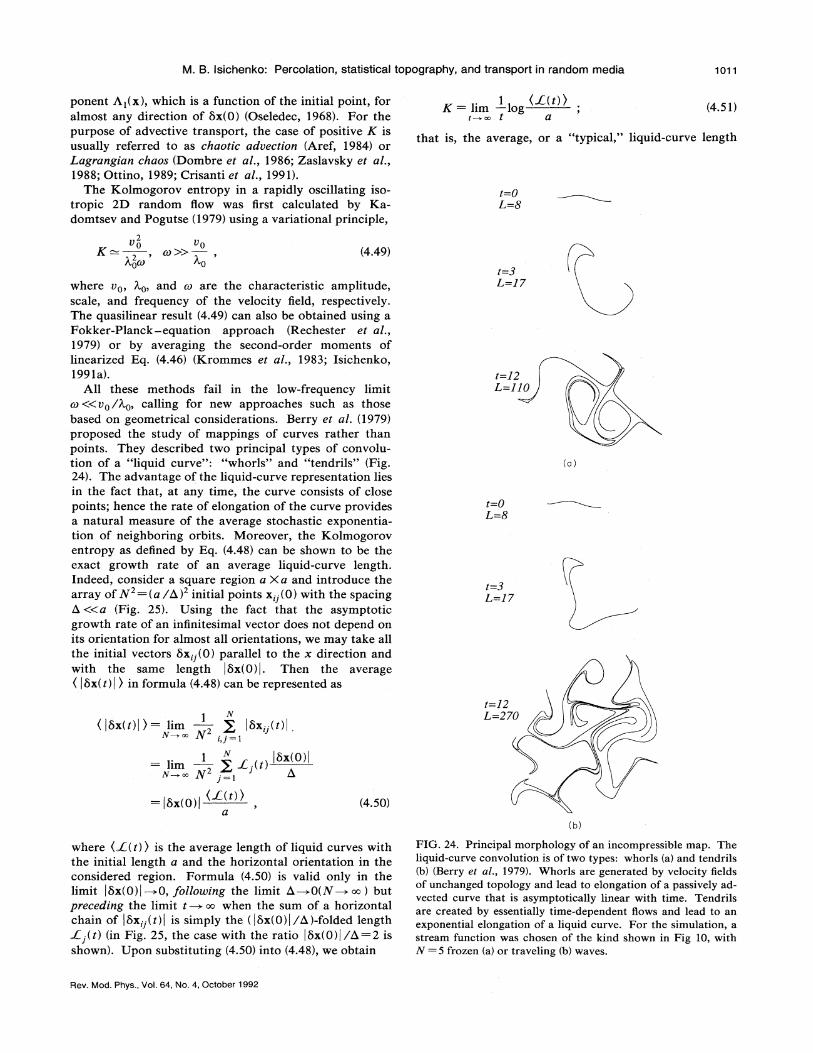
M. B. lsichenko: Percolation, statistical topography, and transport in random media 1011
ponent Ai(x), which is a function of the initial point, foralmost any direction of 5x(0) (Oseledec, 1968). For thepurpose of advective transport, the case of positive K isusually referred to as chaotic aduection (Aref, 1984) orLagrangian chaos (Dombre et al. , 1986; Zaslavsky et al. ,1988; Ottino, 1989; Crisanti et al. , 1991).
The Kolmogorov entropy in a rapidly oscillating iso-tropic 20 random flow was first calculated by Ka-domtsev and Pogutse (1979) using a variational principle,
2vp vp
K=, co))A, 0CO 0
(4.49)
where vp, A,p, and co are the characteristic amplitude,scale, and frequency of the velocity field, respectively.The quasilinear result (4.49) can also be obtained using aFokker-Planck —equation approach (Rechester et al. ,1979) or by averaging the second-order moments oflinearized Eq. (4.46) (Krommes et ai , 198.3; Isichenko,1991a).
All these methods fail in the low-frequency limitco(&vp/A, p, calling for new approaches such as thosebased on geometrical considerations. Berry et al. (1979)proposed the study of mappings of curves rather thanpoints. They described two principal types of convolu-tion of a "liquid curve": "whorls" and "tendrils" (Fig.24). The advantage of the liquid-curve representation liesin the fact that, at any time, the curve consists of closepoints; hence the rate of elongation of the curve providesa natural measure of the average stochastic exponentia-tion of neighboring orbits. Moreover, the Kolmogoroventropy as defined by Eq. (4.48) can be shown to be theexact growth rate of an average liquid-curve length.Indeed, consider a square region a Xa and introduce thearray of N =(a/6) initial points x; (0) with the spacingb. ((a (Fig. 25). Using the fact that the asymptoticgrowth rate of an infinitesimal vector does not depend onits orientation for almost all orientations, we may take allthe initial vectors 5x, (0) parallel to the x direction andwith the same length I5x(0) I. Then the average& I5x(t) I & in formula (4.48) can be represented as
EC = lim —log&&(r)& .
a(4.51)
t=3L=17
t=12L=1'2'0
t=3L=J7
that is, the average, or a "typical, " liquid-curve length
N
&15x(t)l&= lim, y I5x;, (r)I.l) J
= lim, g J', (t)1~
I5x(0)
I
J
(0)l&X(r) &
a(4.50)
t=12L=27
(b)
where &X(t) & is the average length of liquid curves withthe initial length a and the horizontal orientation in theconsidered region. Formula (4.50) is valid only in thelimit I5x(0)I~0, following the limit b.~O(N~ ~) butpreceding the limit t —+ co when the sum of a horizontalchain of I5x;.(r)l is simply the ( I5x(0)l /b, )-folded lengthXj(t) (in Fig. 25, the case with the ratio I5x(0)l/6=2 isshown). Upon substituting (4.50) into (4.48), we obtain
FICx. 24. Principal morphology of an incompressible map. Theliquid-curve convolution is of two types: whorls (a) and tendrils(b) (Berry et al. , 1979). Whorls are generated by velocity fieldsof unchanged topology and lead to elongation of a passively ad-vected curve that is asymptotically linear with time. Tendrilsare created by essentially time-dependent Aows and lead to anexponential elongation of a liquid curve. For the simulation, astream function was chosen of the kind shown in Fig 10, withN =5 frozen {a)or traveling (b) waves.
Rev. Mod. Phys. , Vol. 64, No. 4, October 1992

1012 M. B. lsichenko: Percolation, statistical topography, and transport in random media
(a)
FIG. 25. Relation between the Kolmogorov entropy and theelongation of a liquid curve.
grows at large time as
(X(t) ) =a exp(ICt) . (4.52)
A useful example of such a dependence is given by theobservation that a liquid curve is draped over saddlepoints of the velocity field (Fig. 26) and stretched in theinterseparatrix channels. For a steady flow, this leads toonly a linear growth of the liquid curve via the whorls.When the flow topology is changed, the curve producesexponentiating tendrils via repeated stretching and fold-ing. Consider a flow with a shear structure whose direc-tion is periodically changed. If these changes are slowenough, co ((Uo/Ao, then during the first half of a periodthe curve length is stretched approximately vp /Xp~times, leading to a "fish-bone" structure [Fig. 27(a)].I3uring the second half-period, when the topology of thechannels is changed, each piece of the primary fish bone
FIG. 26. Interaction of a liquid curve with a saddle point of avelocity field. Featured is the hooking of the curve over thesaddle. The dashed line denotes the initial position of thecurve, the heavy solid line is its final state, and the light lineswith arrows show the velocity field.
is stretched into a secondary fish bone, so that theliquid-curve pattern becomes quite intricate [Fig. 27(b)].The process will continue, thereby leading to an exponen-tial growth in the curve length,
VpX(t) =a
XpCi7(4.53)
that is,
UpK =colog
Ape(4.54)
The logarithmic dependence of the Kolmogorov entro-py on the velocity amplitude was numerically observedby Kleva and Drake (1984) in the Aow$=$0[cosx cosy —E sinx cos(y —t)] for fo)) 1. Thespatial structure of the extended streamlines of this flowis similar to that shown in Fig. 27, although cells ofclosed streamlines with the corresponding whorls are alsopresent.
In nonperiodic flows, one expects a stronger exponen-tiation rate, because a continuous distribution of saddlepoints over the level of P and the abundance of separa-trices imply a much faster rate of separatrix reconnec-tion. Gruzinov et al. (1990) studied the stretching andfolding of a curve advected in a monoscale 2D randomflow, a process stemming from the elementary reconnec-tions of the separatrices [Fig. 28(a)]. In terms of theliquid-curve behavior, this results in the multiple drapingof the curve over saddles and its stretching in the chan-nels between the separatrices [Fig. 28(b)]. The mosteScient contribution to the elongation of the liquid curveis made by the channels where the convective revolutionperiod is balanced by the reconnection time of the two
(b)
FIG. 27. Exponentiation of a liquid curve {the dashed line isthe initial position and the solid heavy line is its final position)in a periodically changing shear Aow during the first half-period{a) and during the second half-period {b).
Rev. Mod. Phys. , Vol. 64, No. 4, October 1992
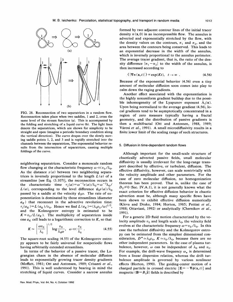
M. B. lsichenko: Percolation, statistical topography, and transport in random media 1013
(a)
((i1
( fVn(x, t)~) ~exp(Kt), t~~ . (4.56)
formed by two adjacent contour lines of the initial tracerdensity n (x, 0) in an incompressible Sow. The annulus isadvected and exponentially stretched by the Qow, withthe density values on the contours, n, and n2, and thearea between the contours being conserved. This leads toan exponential decrease in the width of the annulus,which is inversely proportional to the annulus perimeter.The average tracer gradient, that is, the ratio of the den-sity difFerence ~n, n2~ t—o the width of the annulus, isthen increased according to
(b)
FIG. 28. Reconnection of two separatrices in a random Aow.Reconnection takes place when two saddles, l and 2, cross thesame level of the stream function (a). This is accompanied bythe folding and stretching of a liquid curve (b). The light linesdenote the separatrices, which are shown for simplicity to bestraight and open (imagine a periodic boundary condition alongthe vertical direction). The curve drapes over the slowly mov-ing saddle points 1, 2, and 3 and is rapidly stretched into thechannels between the scparatrices, The exponential behavior re-sults from the intersection of separatrices, causing multiplefoldings of the curve.
neighboring separatrices. Consider a monoscale randomQow changing at the characteristic frequency co « Up/A, p.As the distance s(a) between two neighboring separa-trices is inversely proportional to the length L(a} of astreamline [see Eq. (3.107)], the reconnection occurs inthe characteristic time r, (a }= to 's (a ) /AD= co 'Ao/L(a), corresponding to the level difference /os(a)/Aopassed by a saddle at the velocity Poco. The rate of ex-ponentiation is dominated by those streamlines (diameterax. ) that reconnect in the advective revolution time:
(ar)=xL (ax )/uo. Hence we find L (ax)=(Aouo/co)'and the Kolmogorov entropy is estimated to beK ~uo/L (ax ). The multiplicity of separatrices insideone az cell leads to a logarithmic correction to K, so that
1 /2UO Up UpE = log, co« (4.55)0 A,0CO 0
The square-root scaling (4.55) of the Kolmogorov entro-
py appears to be fairly universal for nonperiodic Qowshaving arbitrarily extended streamlines.
In terms of the behavior of a passive tracer, the La-grangian chaos in the absence of molecular diffusionleads to exponentially growing tracer density gradients(Moffatt, 1981; Ott and Antonsen, 1989; Crisanti et al. ,1991). This is well understood by bearing in mind thestretching of liquid curves. Consider a narrow annulus
Because of the exponential behavior (4.56) even a tinyamount of molecular diffusion soon comes into play tocalm down the raging gradients.
Another effect associated with the exponentiation isthe highly nonuniform gradient buildup due to the possi-ble inhomogeneity of the Lyapunov exponent A, (x).Upon being normalized to the average gradient (4.56), lo-cal gradients tend to be asymptotically concentrated in aregion of zero measure typically having a fractalgeometry, and the distribution of passive gradients isthen a multifractal (Ott and Antonsen, 1988, 1989;Varosi et al. , 1991). A small microdiffusivity results in afinite lower limit of the scaling range of such structures.
5. Diffusion in time-dependent random flows
Although important for the small-scale structure ofchaotically advected passive fields, small moleculardiffusivity is usually irrelevant for the long-range trans-port described by effective, or turbulent, diffusion. Theeffective diffusivity, however, can scale nontrivially withthe velocity amplitude and other parameters. For thecase of zero molecular diffusion, no homogenizationtheorem has been proved. That is, unlike the case ofDO%0 (Sec. IV.A. 1), it is not generally known what theexact criterion for effective diffusion behavior in chaoticadvection must be, although many specific Qows havebeen shown to exhibit effective diffusion numerically(Kleva and Drake, 1984; Horton, 1985; Pettini et al. ,
1988; Ottaviani, 1992) or analytically (Chernikov et al. ,1991).
For a generic 20 Quid motion characterized by the ve-locity amplitude Up and length scale A,p, the velocity fieldevolves at the characteristic frequency co=Up/kp. In thiscase the turbulent diffusivity and the Kolmogorov entro-py can be estimated from the simplest dimensional con-sideration, D =kpup, Sf=Up/kp, because there are noother independent parameters. In the case of plasma tur-bulence, however, co can be independent of A,p and Up.
For example, the drift-wave frequency ~, is determinedfrom a linear dispersion relation, whereas the drift tur-bulence amplitude is governed by various nonlineareffects (Horton, 1990). The guiding-center motion of acharged particle in crossed electric [E=—VP(x, t)] andmagnetic (B=Buz) fields is described by
Rev. Mod. Phys. , Voj. 64, No. 4, October 1992

1014 M. B. lsichenko: Percolation, statistical topography, and transport in random media
dx EXBdt II
=v z+c (4.57)
which corresponds to an incompressible motion acrossthe magnetic field with the stream function
f(x,y, t) =— x,y, zp+ J u)(t')dt', t . (4.58)II
The characteristic frequency, pal=max(co„k~~ui) (wh«e
k[~ —~'9 log//Bz~ ), is thus decoupled from the amplitude
of P. This may lead to the possibHity of both the high-frequency regime (co))up/Ap also known as the quasi-linear limit) and the low-frequency (co «Up/A, p), or percolation, regime of turbulent diffusion (Isichenko andHorton, 1991).
Another example is plasma heat conduction in a mag-netic field with a small random component,B=Bpz+5Bi(x), 58i=VA~~(x)Xz. The equation of amagnetic-field line in the form
dxy 58gdZ 80
(4.59)
Xi =+mve ~ (4.60)
where v, is the thermal velocity of electrons. Particietransport coefficients are also proportional to D (Finnet al. , 1992). The processes of heat conduction in a col-lisional plasma are more complicated, the expression for
involving both the magnetic-line diffusivity D andthe Kolmogorov entropy X (see Sec. IV.B.2).
The above examples inspired studies of turbulentdiffusion in two dimensions, with the characteristic Aowfrequency co considered to be a free parameter. In thehigh-frequency (low amplitude) limit, co ))Up /A, p, theeffective diffusivity is insensitive to the topology ofstreamlines because the fIow is changed in the correlationtime co —that is, well before a tracer particie is dis-placed by a distance A,0. This corresponds to the so-called quasilinear approximation, which consists, rough-ly, in the following. Represent the tracer density n {x,t)as the sum of a smoothed component X, evolving slowlyin both space and time, and a Auctuating component ndue to the driving velocity field, and then substitute thesum into Eq. (4.1). Upon separating oscillatory and aver-aged parts, we have
is equivalent to Eq. (4.46) with the stream functionf(xi,z)= A~~(xi, z)/Bp and the coordinate z standing fortime. The turbulent diffusivity stemming from Eq. (4.59)is known as the magnetic-field-line diffusivity D (Rosen-bluth et al. , 1966). This quantity has the dimensionalityof length. In a collisionless plasma, the diffusive walk ofmagnetic lines causes an enhanced electron thermal con-ductivity across the background magnetic field(Krommes, 1978; Rechester and Rosenbluth, 1978; Ka-domtsev and Pogutse, 1979)
where the averaging is taken over "small scales" and"fast time" or, alternatively, over an ensemble of Aows.Upon integrating Eq. (4.61) over fast time and substitut-ing n into (4.62), we obtain
dN/dt=V; f dt'(U;( xt)Uk(x, t')}VkX; (4.63)
that is, the turbulent diffusivity is given by the time in-tegral of the Eulerian velocity correlation function,which corresponds to the estimate
2V0 V0m))
0(4.64)
In the above derivation, the limits of the applicability ofthe quasilinear approximation are swept under the rug.The comparison with the Taylor formula (4.5), involvingthe Lagrangian velocity correlator, reveals the inequalitydisplayed in Eq. (4.64) specifying the small difFerence, ontime scales of interest, between the Eulerian velocityv(x(0), t) and the Lagrangian velocity v(x(t), t).Mnemonically, one can view the quasilinear approxima-tion as the neglect of the v(x, t) dependence on x makingthe particle orbit equation (4.2) linear
In the opposite, low-frequency limit co « Up/Ap, atracer particle can move along an almost steady stream-line to a large distance before the Qow pattern haschanged appreciably. Consider a monoscale, random,slowly varying two-dimensional fIow. The mixing length
is defined as the maximum coherent particle displace-ment that occurs in the lifetime r(g ) of the convectioncel1.
L (g ) =Upr(g ) (4.65)
[compare with (4.38)]. The lifetime r(a) of an a cell is thetime of unrecognizable change (for example, doubling thediameter) in the contour it( jyx, t) =h with the initial di-ameter a. Such a change is undergone through the con-tour reconnection process [Fig. 28(a)]. The reconnectiontakes place when the saddles corresponding to neighbor-ing separatrices come through the same level. An essen-tial change in the shape of the convection cell occurswhen the saddles pass the level difference5g=itpw(a)/Ap corresponding to the width of the cellw(a) given by Eq. (3.45). As the level of a saddle pointchanges at the characteristic rate /pep, the lifetime of theconvection cell is estimated to be
5g w (a)ra =/pe A.pCO
(4.66)
Upon substituting Eq. (4.66) into (4.65), we find the inix-ing scale
v/(vdh +1)
(4.67)A,063
The turbulent diffusivity is then estimated similarly to(4.40),
an(x, t)/at = —v(x, t)VX(x, t),BK(x, t)/'dt = —(v{x,t)Vn(x, t) },
(4.61)
(4.62)(4.68)
Rev. Mod. Phys. , VGI. 64, No. 4, October 1992

M. B. Isichenko: Percolation, statistical topography, and transport in random media 1015
Thus the percolation scaling of the turbulent diffusioncoefficient is given by (Gruzinov et al. , 1990)
' 1/(vdh+1), ~ 3/gp
Up Up
Upcg «
p
10
(4.69)
Ottaviani (1992) studied the effective diffusion in atime-dependent 2D flow numerically. He used a quasi-periodic stream function with %=64 standing wavesmodulated by random Gaussian amplitudes with a vari-able correlation time co . In the high-frequency limitthe quasilinear diffusivity (4.64) scaling was demonstrat-ed. In the low-frequency limit, the observed scaling ofthe turbulent difFusivity, D* ~ f~ ",'.was close to, butstill distinct from, the dependence D'~go~' predictedby the formula (4.69) (see Fig. 29). The finite number ofwaves is likely to be responsible for the discrepancy, be-cause a quasiperiodic potential has a nondecaying (quasi-periodic) correlator and certainly does not belong to theuniversality class of uncorrelated percolation. It is notclear to what extent the N-wave quasiperiodic potentialscan serve a good model of monoscale random potentials,although it is plausible that in the limit N~ ao the modelmust be good.
The low-frequency/large-Peclet-number turbulentdiffusion theory, which employs statistical topographyanalysis, was extended in several directions. Kalda(1992) studied the general case of multiscale, time-dependent, incompressible 2D flow, including the effectof molecular diffusion, where numerous effective diffusionregimes have been identified.
Gruzinov (1991) considered the effective diffusion in a
weakly compressible random flow
v=VQ(x, y, t)Xz+sVQ(x, y, t) . (4.70)
The last term in (4.70), which models a non-Hamiltonianfriction experienced by a drifting guiding center, makesparticles move at a small angle c «1 with respect to thecontours of f. Random walk in fields with finite diver-gence was also discussed in the context of the vortexmotion in inhomogeneous superconducting films (Trug-man and Doniach, 1982) or random-hopping models indisordered solids (Derrida and Luck, 1983; Fisher, 1984;Kravtsov et al. , 1986). The compressibility of advectingflow results in the occurrence of limit cycles and stablefoci, which attract and trap tracer particles (Fig. 30) untilthey are released due to molecular diffusion or flow timedependence destroying the traps. So the diffusion processresults from the particle flights from one trap to another.In the low-frequency limit, these flights are approximate-ly along the contours of g(x,y, t) and may be quite long(Levy fiights; cf. Shlesinger et al. , 1987). For the monos-cale compressible fiow (4.70), the effective diffusivityscales as
—vdg /(~dg +1) 0D =k&coo, , «c, «1 .
Up(4.71)
For smaller E, the effect of compressibility is unimportantand D* is given by formula (4.69). In the case of time-independent compressible flow with finite moleculardiffusivity Dp, the effect of traps can result in an ex-ponentially small effective diffusivity D*.
Yushmanov (1992) studied the neoclassical diffusion in
a turbulent plasma. Mathematically, this problem wasreduced to chaotic advection in a random 2D flow with atemporally varying average component. The average ve-
locity component in an equation similar to (4.57) results
10- Quasilinear /
10—
10'Closure
+
10'
io
1010 i0 10 10 10
K10
l
i0 10
FIG. 29. Dependence of the turbulent diffusivity on the "Kubonumber" E =Up/(Apso) at A,p=Up=1 (Ottaviani, 1992). Thedashed line D o- K represents the diffusion behavior in the high-frequency limit K & 1 and corresponds to the quasilinear scaling(4.64). The low-frequency behavior shows a systematic declinefrom the prediction of a Markovian closure theory (solid line;for a recent discussion see Fradkin, 1991).
FIG. 30. Streamlines of weakly compressible Aow (4.70) with
e =0. 1 and 1(ix,y) the same as in Fig. 10.
Rev. Mod. Phys. , Vol. 64, No. 4, October 1992

1016 M. B. Isichenko: Percolation, statistical topography, and transport in random media
from bounce oscillations of particle guiding centers dueto the toroidal geometry of a tokamak. Causing alternat-ing opening and closing of random streamlines, such aneffect leads to the onset of effective diffusion at zero col-lisional diffusivity.
6. Anomalous diffusion
Effective diffusion in an advection-diffusion system re-sults from asymptotically decaying correlations in theparticle trajectory. This "loss of memory, " which is dueto molecular diffusion, Lagrangian chaos, or both, occursin a finite Inixing time ~ . On a time scale t (~ theadvection-diffusion transport can exhibit more sophisti-cated, "anomalous" behavior (Bouchaud and Georges,1990). In particular, the root-mean-square particle dis-placement can scale differently from the standard squareroot of time,
(4.72)
where gA —,' is the exponent of anomatous diffusion We.
use the notation g for the anomalous diffusion exponentin place of the more standard notation v, which is al-ready used for the correlation length exponent in percola-tion theory.
Similarly to the scalings for effective diffusivity D' inincompressible Ilows, the exponent g also forms certainclasses of universality, including continuous classes (thatis, depending on the flow specrum). In a compressibleliow (V vAO), however, the universality may breakdown, because the presence of "traps" such as stable fociof the flow (Fig. 30) results in qualitatively new transporteffects. This can lead to the intriguing continuous depen-dence of the exponent g on the degree of compressibility(Bouchaud and Georges, 1990).
Anomalous diffusion can also take place in nonintegr-able Hamiltonian systems where the velocity field is thephase-space Aux (Afanasiev et al. , 1991; Swagerl andKrug, 1991). In some cases the onset of anomalousdiffusion is similar to a percolation threshold (Chaikov-sky and Zaslavsky, 1991).
One might suppose that the coordinates x(t) of a parti-cle undergoing an anomalous diffusion (4.72) can bemodeled by a fractional Brownian function B&(t). In thegeneral case, however, this is not true, as the incrementsof x( t) may not be Gaussian (Ball et al. , 1987; Bouchaudet al. , 1990). The probability distribution functionn (x, t) of x, for n (x,O)=5(x), is given by the solution ofthe complete advection-diffusion equation. In the long-time limit, one can expect a self-similar behavior in theform
which becomes Gaussian only in the case of a standardBrownian motion (g= —,'). Still, for a sufficiently rapidlydecreasing f (u) the distribution (4.73) is qualitativelysimilar to the Gaussian probability distribution function,so that a fractional Brownian motion can serve as areasonable model for anomalous diffusion. Specifically,the fractal dimension D of the particle trail is given byformula (3.3S), whose derivation is not hinged on theGaussianity of x(t):
D =min(1/g, d), (4.75)
where d is the corresponding space dimension.Two physically different regimes of anomalous
difFusion should be distinguished between: superdiffusion(g) —,
') and subdiffusion (g & —,
' ). Bouchaud and Georges(1990) (see also Zaslavsky, 1991) identify the statisticalmechanisms of anomalous diffusion in the example ofgeneralized random walks, where a random walker un-dertakes a random step of length I;=x;+,—x, , upon arandom waiting period w, =t; —t, , For independentand narrow distributions of I; and ~;, the standarddiffusion is recovered. Superdiffusion can result from awide distribution of I; (meaning sufficiently slowly decay-ing probability of large steps) or from persisting correla-tions between successive steps, whereas subdiffusion re-sults from a wide distribution of waiting times. In whatfollows, we attempt to exemplify these mechanisms onthe grounds of passive advection.
a. Superdiffusion
One can imagine Bows with long-range velocity corre-lations resulting in a "persistent" particle orbit, whose atleast partial memory of the previous history lasts forever:
According to the Tatarinova et al. (1991) andthe Avellaneda and Majda (1991) theorems, in the pres-ence of finite molecular diffusivity such fIows should havean unbounded vector potential P(x, t). The simplest ex-ample of superdiffusion was described by Dreizin andDykhne (1972). Consider a shear liow with the velocitytaking at random two constant values, u =u„(y) =+uo, instrips of width A, o (Fig. 31). The average velocity for al-most every realization of this How is zero, while the
n(x, r) =Ct &df ( lxl /r &), (4.73)
where an isotropic transport is assumed. T'he apparentlytypical behavior is described by the Fisher (1966) modelof a random self-avoiding walk,
f(u)~exp( —u' " &'), (4.74)FIG. 31. Randomly directed shear Aow with zero mean veloci-
ty but with a Brownian-type stream function.
Rev. Mod. Phys. , Vol. 64, No. 4, October 1992

M. B. Isichenko: PercoIation, statistical topography, and transport in random media 1017
stream function g(y) = f ~ov (y')dy' is unbounded at
y —+oo. By time t, a tracer particle gets quasiuniformlydispersed in the y direction over the distanceA, =(Dot)'/, covering approximately N=A~/ko Aow
strips. Given the random distribution of velocity direc-tions, one can expect approximately X', say, left-directed strips in excess of right-directed ones. The frac-tion of time the particle spends in these excessive (left-directed) strips is of order N'/ /N =N '/ . Hence theexpected (rms) particle displacement in the x direction isgiven by
=u tN ' =u (A, /D )' tX (4.76)
a superdiffusive behavior (g= —,' ) 1/2).
A continuum generalization of this steplike Aow is aone-dimensional random stream function P=g(y), withthe spectrum fi = go(A, IA,o), A, )A,o, 0 & H & l. [The ex-ample of Dreizin and Dykhne (1972) corresponds toH =
—,'.] The velocity spectrum of such a Aow,
uz=uo(A, /Ao) ', also implies zero mean velocity:(u ) =v), =0. The superdiffusion law is similarly ob-tained as
A,,(t) =QD,t,(t) —
u t —u (g2/D )(i —H)/2t()+H)/2
x A (t) 0 0 0
(4.77)
t&A,O2/D, .
The averaged transport equation describing super-diffusion (4.77) cannot be cast into a local form; however,the average tracer density ( n ) may be representedasymptotically as the ensemble average of the solutionsof the simple equation
dn /dt =J7t 3(n IBx (4.78)
where % is a random coefficient with known distribution(Avellaneda and Majda, 1990).
Bouchaud et al. (1990; see also Redner, 1989 andCxaveau and Schulman, 1992) considered an isotropic 2Dgeneralization of the random-directional shear Aow —the"Manhattan system"
P(x,y) =g, (x)+g,(y) (4.79)
(see Fig. 32). Suppose each component of the streamfunction (4.79) has a power spectrum with the exponentH &0: it)) ~ iP. Anomalous diffusion in such a Aow canbe obtained similarly to Eq. (4.77). Due to the statisticalisotropy of the system, the rms displacement A,(t) is self-consistently coupled to the result:
FIG. 32. Isotropic random Aow of the "Manhattan-grid" typeshown by the superposition of two mutually perpendicular ran-dom shear Qows.
Cxiven the way result (4.81) has been derived, one canexpect its wider generality. In fact, the superdiffusive law(4.81) is valid not only for a Manhattan Aow, but also foran arbitrary random stream furiction with the isotropicpower spectrum g&~A, (Isichenko and Kalda, 199lc).The validity of (4.81) for a two-dimensional random Aow,however, is restricted by the inequality 0 & H & —,", (regionC in Fig. 23). Formula (4.81) also extends to the three-dimensional case. Koch and Brady (1989; see also Brady,1990) considered random, steady 3D Aows with the alge-braically decaying velocity correlator(u,.(x)u~(x+p)) ~|)~~p~ ~ and found the superdiff'usivetracer dispersion (4.72) with the exponent
0&y&2.2(4.82)y+2'
The velocity covariance ~~p~
~ corresponds to the spec-trum ui ~A, ~ [see Eqs. (3.9)—(3.13)] and hence to thevector potential P(x) /L-spectrum exponent H =1—y/2.Then Eq. (4.82) is equivalent to (=1/(2 —H), in accor-dance with Eq. (4.81).
The marginal case H =0 requires special analysis be-cause the delta variance of the stream function,&(p)=([g(x+p) —f(x)] ), behaves as logp forAo &p & A, . For A,(t) & A, the stream function, as sam-
pled by tracer particles, is logarithmically unbounded.This leads to a new regime of logarithmicalsuperdiff'usion (Kravtsov et al. , 1986; Bouchaud et al. ,1987),
7 (t) =Nb, '"(A(t)) t=QP, t log' '(g, t/A, ,'),A(t)=v)(, )t . (4.80) (4.83)
It follows that]. /(2 —0)
UotA, (t) =A,o
Xo
Ao
0(4.81)
At H =—,' one has the superdiffusion exponent
g= 1 /(2 —H) =—,' (Bouchaud et al. , 1990). A, (t)=Di(, )t . (4.84)
The superdiffusive laws (4.81) and (4.83) do not exhaustall anomalous regimes in 2D random, steady power-spectrum Rows. Another superdiffusive regime in a mul-tiscale Aow corresponds to the random walk with theself-consistently determined partial diffusivity (4.42)
Rev. Mod. Phys. , Vol. 64, No. 4, October 1992

1018 M. B. Isichenko: Percolation, statistical topography, and transport in random media
Substituting formulas (3.74) and (3.80a) into
Di =DoL(A, )/tu(A, ), we obtain Di, ~ A, ";hence (Isi-chenko and Kalda, 1991c)
i1/(2+H —D~ )
A(t)=Ao A,,& A, (r) &min(g, X ),0
(4.85)
where g is the solution of Eq. (4.38). For H & 1 we have
1
2+H —D~
7 1
10H +4 2
This superdiffusive regime is possible for H & ——', in theregion C in Fig. 23. It is interesting to note that, for——', &H & —,'„Eq. (4.69) predicts the root-mean-squareparticle displacement to grow faster than linear with time(g) 1), that is, with an acceleration ("superballistic" re-gime).
It must be emphasized that, by definition, regime (4.86)corresponds to a "typical" initial position of a tracer par-ticle in a given Aow, that is, on a streamline with the sizeof order A,o, hence it cannot be obtained by averagingover the initial position or the ensemble of Aows. Suchan averaging would lead to something different due to thesignificant transport role played by scarce long stream-lines. These lines wi11 eventua11y dominate the transportafter effective diffusion sets in, but one should not neces-sarily perform the ensemble average when studying tran-sient anomalous behavior for a specified initial condition.To exemplify this remark, consider a monoscale (Ao) 2Dsteady Aow in the absence of molecular diffusion(Do =0). Then for almost any initial position the particledisplacement is forever bounded by the diameter a of thecorresponding streamline; typically, a=i,o. Denote byx (a, r) the particle displacement averaged over a time in-terval [t,2t]. This displacement clearly behaves as
&,(u, r/A. ,) ", u, r L&(a) =k,( /aA, ,) ',x(a, t)= '
a, uot)L(a),
a subdift'usive behavior [g—I/(2dl, )=2/7] with an un-
bounded displacement. A subdiffusive behavior was nu-
(4.87)
where d& =—,' is the fractal dimension of the monoscale
streamline. For a single particle released on a longenough streamline, the first equation (4.87) predicts asuperdiffusive displacement (g= 1/dh =4/7). However,the average square displacement over the ensemble ofBows or, equivalently, over the initial conditions, corre-sponds to a subdiffusive behavior. Upon averaging thesquare expression (4.87) with the help of the distributionfunction (3.47) of the streamlines, we obtain
1/d~
(A, (t)) =J x (a, t)F(a) =Ao, (4.88)~0 a ko
merically observed by Kraichnan (1970) for the case ofan ensemble of 20 incompressible steady Aows. Thissubdiffusion clearly has little to do with the generic be-havior of a passively advected particle in a particularrealization of the Aow. Still, for the corresponding con-ductivity problem (for the correspondence, see Sec.IV.B.3.b), the ensemble-averaged anomalous difFusion inthe advection-difFusion system may be relevant, upon be-
ing translated into a size effect —that is, the dependenceof the specific conductance of a sample on its size (Dreiz-in and Dykhne, 1972; Isichenko et al. , 1989; Isichenkoand Kalda, 1991a). Here the interesting problem of therelation between the ensemble-averaged transport, on theone hand, and the typical behavior for a given realizationof a disordered system, on the other hand, is only posedwithout being duly addressed.
Perhaps the most important implications of anomalousdifFusion concern real turbulent (time-dependent) flows.The Richardson law (4.6) means, by definition of Dz, thatthe root-mean-square relative displacement of advectedparticles behaves as A,(t)=(D&(,)t)'; hence
k(r) ~ t'~' . (4.89)
Q) g—Q)0
koAo(A. & A, (4.90)
In a pure fiuid turbulence, one would have rui =ui/A, ,
that is, G =2—H. For the turbulence of Rossby waves in
a rotating fiuid, drift waves in plasmas (Hasegawa and
Mima, 1978; Hasegawa et al. , 1979), or other systems
having a characteristic velocity V such as the phase ve-
locity of linear waves, regimes with coi = V/A, are possi-
4The standard form for this spectrum is usually given in termsof the energy spectral density, E(k) ~k . The relation be-tween E (k) and Ez ~ u z is given by Ez = J. . .E (k)dk ~ A, ~'.1/A,
The Richardson superdiffusion (4.89) is naturally ob-
tained from the Kolmogorov-Obukhov spectrum (Kol-mogorov, 1941; Monin and Yaglom, 1971, 1975; Roseand Sulem, 1978; Batchelor, 1982) ui ~A, '~ upon using
the relation A(t)=ui(, )t. Indeed, ui is the characteristicvelocity diff'erence between two points that are a distanceA, apart from each other. The superdiffusion law (4.89)was derived by Obukhov (1941) from a dimensionalanalysis similar to the one that led Kolmogorov (1941) tothe A,
'~ (H =—', ) velocity spectrum. The detailed discus-
sion of the relation between the Kolmogorov spectrumand the Richardson superdiffusion was given byBatchelor (1952).
In the case of a decreasing velocity spectrum,
ui ~ A, ',H & 1, a nontrivial absolute superdifFusion is
also possible. Time dependence can be introduced in theform of the characteristic frequency co& at which the A,
component ui (x, t) of the velocity field is evolved:—G
Rev. Mod. Phys. , Vol. 64, No. 4, October 1992

M. B. Isichenko: Percolation, statistical topography, and transport in random media 1019
ble, that is, G =1. The superdiffusive law for arbitrary6 )0 and H & 1 can be obtained as follows. The dis-placement of a tracer particle, released in the Aow att =0, is governed at time t by the Bow component withA, =A, *(t) determined from the equation co + t = l.
A, (t)Indeed, at H & 1 longer scales [A, &)A, '(t)] have smallervelocity, whereas shorter scales [A, «A, '(t)] have fast-oscillation velocity components: co&t ))1. In the absenceof other scales, these oscillations would lead to the tur-bulent diffusivity given by formula (4.64):Dz= U&2/cg&~A, G+ 2. If Dz increases with growingA,—that is, 6)2 —2H —then the A, *(t) velocity scaledominates the tracer motion. In this case, we can writethe root-mean-square displacement A, (t) in two equivalentforms, A(t) =U&..,.t =(Dz~„,t)'~ . Thus we obtain
A,(t)= (co t) + " 6 &2—2H &0 . (4.91)COp
In the opposite case, G &2—2H, the small-scale velocitypulsations dominate the particle motion, leading to theturbulent diffusivity D =Uo/coo. The validity of result(4.91) in two dimensions is further restricted by the in-
equality 6 ~ 2 —H to ensure the absence of an additionalintegral of motion —the adiabatic invariant of the streamfunction g[x(t),y(t), t]—which is approximately con-served at co~&&u&/A. . The low-frequency transport in atwo-dimensional multiscale time-dependent Aow is morecomplicated and requires the statistical topographyanalysis of particle orbits (Kalda, 1992).
Osborne and Caponio (1990) studied numerically pas-sive transport in a 20 time-dependent random How withspectral exponents G=1, —,
' &H &3. They found thesuperdiffusion exponent g to behave as g=H, for—,' & H & 1, in accordance with Eq. (4.91).
Notice that in the case of a turbulence with the eddy-revolution characteristic frequency ~&=v&/A, , that is,6 =2 H, Eq. (4.91) lead—s to the superdiffusive exponent/= 1/(2 —K), the same as in Eq. (4.81) describing thesuperdiffusion in steady fiows.
Avellaneda and Majda (1990) considered anomalousdiffusion in random, unsteady shear flows, U =U„(y, t).They identified several regimes of the tracer behavior andestablished the equations describing the average density(n ).
The anomalous diffusion scalings, such as in Eqs.(4.81), (4.85), and (4.91), can be used to recover turbulentspectra from the observed tracer motion, such assatellite-tracked buoys deployed in the ocean (Osborneet al. , 1986; Brown and Smith, 1991). To do so, one canuse either complete time-coordinate records [t, ,x;,y, ] oronly the trail Ix, ,y; ], whose fractal dimension D is relat-ed to the anomalous diffusion exponent g by formula(4.75). However, for deciphering turbulence spectra
with H ) 1, tl.e information stored in the relativeparticle dispersion has to be used.
Another manifestation of a self-similar (power-spectrum) turbulence is the fractal structure of the iso-
scalar surfaces, that is, the surfaces where the density ofa passive scalar takes a constant value. Constantin et al.(1991) give theoretical expressions for the fractal dimen-sion of isoscalar surfaces, D;„=2+H/2, in the internalregion of a turbulent spot, and D,„=1+H, near theboundary of a turbulent jet, where v& ~ A,
' is the veloc-ity spectrum. These predictions agree with experimentaldata (Sreenivasan and Prasad, 1989; Sreenivasan et al. ,1989; Constantin et al. , 1991). Recent experiments onturbulent diffusion, superdiffusion, and fractal behavioralso include those conducted by Swinney and Tam (1987),Ramshankar et al. (1990), and Ramshankar and Ciollub(1991). Some other fractal and multifractal properties ofpassive scalars are discussed by Mandelbrot (1975b),Hentschel and Procaccia (1983a), Ott and Antonsen
. (1988), Voss (1989), Vulpiani (1989), Fung and Vassilicos(1991),and Varosi et al. (1991).
h Subdiffusion
The superdiffusive (persistent) random walk does notexhaust the variety of anomalous diffusion regimes in in-cornpressible Aows. The subdiffusive (antipersistent)tracer motion with g& —,
' is also possible (Pomeau et al. ,
1988; Young, 1988; Young et al. , 1989). In a time-independent flow, such behavior arises from the tracerparticles resting in closed pockets of recirculation. Oncein a region of such closed streamlines, the particle residesthere for a time before proceeding with its propagation.This waiting time is governed by molecular diffusion andhence is a random quantity with a wide distribution. Theresulting retarded (g & —,
') dispersion (Montroll and Scher,
1973) is quite similar to the diffusion on comblike struc-tures (Fig. 33; Havlin and Ben-Avraham, 1987). The sys-tem of regular convection rolls (Fig. 20) is equivalent to acomb whose base represents the diffusive boundary layersand whose teeth correspond to the inner area of the con-vection cells. To complete this analogy, one should posi-tion the teeth, Ao long, the distance wb=i, + '~ (I'
go/Do &) 1) apart —from each other and should ascribea diffusion coefBcient of the order of the moleculardiffusivity Dp to the whole structure. Such a representa-tion of the transport properties of liow (4.22) is valid onthe time scale t &)A,o/Uo, when (a) the boundary-layerstructure of transport has set in and (b) the tracer disper-sion inside the convection rolls can be described by the
r rr rr rr rr rr rr rr rr rr rr rr rr rr rr rr rr rr rr rrrr rr r
FICx. 33. Diffusion comb corresponding to a periodic array ofconvection rolls.
Rev. Mod. Phys. , Vol. 64, No. 4, October 1992

1020 M. B. Isichenko: Percolation, statistical topography, and transport in random media
averaged one-dimensional cross-stream diffusion equation
an(J, t) a an (J, t)at aJ aJ (4.92)
D (J)=Do f l vol dl g I vol 'dl, -(4.93)
where the integrals are taken around the streamline (Isi-chenko et al. , 1989; Young et al. , 1989).
Suppose a small spot of dye (passive tracer) is deposit-ed at t =0 close to the separatrix mesh of a periodic ar-ray of vortices (Fig. 20) corresponding to the base of thecomb (Fig. 33). Consider time scalesA,o/vo« t «A, o/Do. Then the dye invades a distance(Dot)'~ along the teeth. The fraction I'(t) of "active"particles —that is, those residing on the base and deter-mining the long-range tracer dispersion —decreases withtime as
F(t)=(D t) i/2 (4.94)
instead of the full 2D advection-diffusion equation (4.1).In Eq. (4.92), n(J, t) designates the tracer density aver-aged over a streamline g(x,y) =const with the area J in-side it. The idea of such averaging stems from the per-turbation theory of nearly integrable Hamiltonian sys-tems (Arnold, 1978), where one switches from the phase-space variables (x,y) to the action-angle variables (J,P)of the unperturbed (integrable) motion. The action-diffusion coefficient D (J) is given by
diffusivity, and IC(r) is an integral kernel satisfying thenormalization condition
f K(~)d7=1 .0
(4.98)
Zaslavsky (1992) phenomenologically suggested using ageneralization of Eq. (4.99),
f (x, t)= [l)(x)f (x, t)],0(4.100)
The sense of Eq. (4.97) is that the tracer fiux is deter-mined solely by the density f in the diffusive boundarylayers and the effective diffusivity D (right-hand side),while the left-hand side specifies the change in the aver-age tracer density (n ) = joK(t ~)f (x—, r)d~. Thelatter is obtained from f via a linear integral operatordescribing the tracer invasion into a convection cell. Inthe limiting case t ))~, where the mixing time7 —A0/D0 is the characteristic time of the convergenceof integral (4.98), the kernel E can be replaced by a deltafunction; hence (n ) =f and the effective diffusion equa-tion is recovered from (4.97). In the opposite case,A, o/vo « t «r, the kernel behaves as a power,&(r)=(r ~) ', and the operator on the left-hand sideof Eq. (4.97) becomes the operator of fractionaldifferentiation [see Eq. (3.36)]:
1/2
f =D*v'f . (4.99)Bt
In terms of the random walk of a single particle, Eq.(4.94) yields the fraction of time spent on the comb base.Then the propagation rate along the base coordinate b isgiven by
b'(t) =F(t)D, t =iv, (D,t)'~' . (4.95)
This corresponds to the root-mean-square displacementin real space (Havlin and Ben-Avraham, 1987; Pomeauet al. , 1988; Young et al. , 1989)
~0A.(t) =b(t) =(A,~~,t)'" (4.96)
a subdiffusive law (g= —,') sometimes referred to as "dou-ble diffusion" (Kroinmes et al. , 1983). Such tracer be-havior is valid for nonvanishing velocity on the separa-trix mesh (free-slip boundary condition). For no-slip (rig-id) boundary, where the velocity falls linearly to zero, onehas g= —,
' (Pomeau et al. , 1988; Young et al. , 1989), a be-havior that was confirmed experimentally (Cardoso andTabeling, 1988).
Not only the rms displacement scaling but also thegoverning equation for the tracer envelope can be estab-lished for periodic Aows. The general form of this equa-tion was derived by Young et al. (1989):
tK t —w x, z d&=D*V x t, 497
Bt 0
where f is the tracer density on a separatrix consideredas a function of "slow" coordinate x, D is the effective
to describe an arbitrary anomalous diffusion with
g =13/a.As the nonlocal time operator i/a/at commutes with
the space operator V, one can write the consequence ofEq. (4.99) in a local differential form,
D 42
Bt 7T
V4 (4.101)
~Those of Eq. (4.99) with D* substituted by —D*.
which emphasizes the term "double diffusion. " The sim-
plicity of (4.101) is, nevertheless, deceptive. While in-
cluding all solutions of the nonlocal equation (4.99), thelocal double-diffusion equation (4.101) has many extrane-ous solutions that well manifest themselves in a stronglyunstable behavior of Eq. (4.101): A monochromatic solu-tion f ~exp( icot+ik x) g.row—s with time exponential-ly, co=ik "~ D* /m, whereas our intuitive conception of(sub)diffusion suggests a behavior of f that smoothes outinitial inhomogeneities.
Subdiffusive behavior is also possible in random veloci-ty fields (Isichenko and Kalda, 1991c). As in regular con-vection cells, this behavior is transient (t &r ) and takesplace for special initial conditions, namely, for the initialtracer spot deposited in a mixing convection cell.(Remember that the mixing convection cells of the size
play the role of boundary layers. ) The difference be-
Rev. Mod. Phys. , Vol. 64, No. 4, October 1992

M. B. Isichenko: Percolation, statistical topography, and transport in random media 1021
Bn 1 8 DL( )Bn
at L(x, ) ax, ' ' ex,(4.102)
tween random Bows and regular Bows lies in the appear-ance of their equivalent loopless structures. Due to thepresence of numerous separatrices in a random Bow, thetracer fills up the holes in a g cell topologically non-trivially, as on each separatrix the converging diffusionfront breaks into two (in a nondegenerate case; see Fig.34). Hence the equivalent "diffusion comb" of a randomRow has branching teeth and looks like a thicket (Fig.35). The rate of filling up the branches of these trees canbe found using the topographic properties of randomAows.
Introduce the "action distance" xJ across the stream-lines according to dJ =+L (xJ)dxJ, where L (x~) is thelength of a closed streamline and J is the area inside thisline. The action-diffusion coefficient (4.93) being estimat-ed as D(J)=DOL (xz), one can rewrite Eq. (4.92) interms of the action distance xJ ..
FIG. 35. Diffusion comb of a random How, which looks like athicket. The subdiffusive propagation along the "ground" (net-work of mixing convection ce11s) stems from the delay caused byrandom walk in the "bushes. "
ed region inside one g cell, introduce a new topographicexponent 5, which can be called "dimension of thedifFusion tree": S(xz) ccxJ. Using the matching condi-tions S[to(g )]=L(g )w(g ) [where L(g ) is the per-imeter (3.43) of the g cell] and S(AO)=g (all the holesare filled up by t =r, when xJ =A,o), we find
0Pl
0(4.103)
Consider time scales w (g )/Do« t «r~. Then thediffusion front invades the action distance xJ(t) =+Dotalong each branch of the diffusion tree. To calculate thetotal area S (xJ ) (in physical space) covered by the invad-
Hence the segments of the "diffusion tree" (Fig. 34) canbe measured in the action-distance units, with thediffusivity along the branches of order Dp.
Consider a monoscale uncorrelated, random, steadyAow with the characteristic scale A,p. The action distancebetween the external boundary of an a cell and the inner-most point of a hole in the cell can be calculated as thesum of the widths (3.45) of the nested cells of diameterA,0, 2A,p, . . . , a. For any a )&Ap this sum is estimated tobe A,p. It follows, in particular, that the action distancebetween two arbitrary points on the (x,y) plane is bound-ed by a constant of the order of A,p. Hence the mixingtime in the monoscale fIow equals
5=1+v(2 —dh)= —', . (4.104)
St~ 0 I »,S(+Dot )
(4.105)
The tracer propagation along the comb base is given byb (t)=F(t)Dot, and, as the distance w(g ) between thetreelike teeth of the comb corresponds to the physicaldistance g, we obtain
DotA(t)=b(t)
The fractional value of the tree dimension 6 between 1
and 2 indicates that, while the complete 2D description(4.1) is redundant, purely one-dimensional actiondiffusion
oversimplifies
the transport in topologicallycomplex Aows.
The rest of the calculation essentially repeats that forthe simplest nonbranching diffusion comb, whose dimen-sion 5 is unity. The fraction of active particles lying onthe base of the comb is
w(g )&t &Vm
Dp(4.106)
where the subdiffusion exponent for 2D monoscale ran-dom Row equals
1 5 1
2 4 6(4.107)
FIG. 34. Diffusion tree (branches shown in heavy lines) corre-sponding to passive transport in a topologically complex Aow.For a nondegenerate How each separatrix divides the plane intotwo inner regions and one outer region; hence all branchingpoints on the tree are Fpoints.
The "triple diffusion, " Eqs. (4.106) and (4.107), can alsobe described by a nonlocal integro-differential equationinvolving the operator (8/Bt)'~ .
The generalization of the above result to the case ofmultiscale Bows is easily done for the monoscale correlat-ed spectrum with the exponent —1/v&H &0. In thiscase one simply substitutes the percolation exponents vand dh in Eq. (4.104) by their correlated percolation
Rev. Mod. Phys. , Vol. 64, No. 4, October 1992

1022 M. B. Isichenko: Percolation, statistical topography, and transport in random media
counterparts (4.44). As a result, we have the dimensionof the diffusion tree
(4.108)
and the subdiffusion exponent
1 62 4
2+H —D„5H +24H 14H
(4.109)
The subdiffusion law (4.106)—(4.109) is valid for——'~H & ——' where 0&g~ —'.
4 g 7 6'
B. Conductivity of inhornogeneous media
The problem of the average characteristics of spatiallyAuctuating dielectrics and conductors is as old as electro-dynamics itself (Maxwell, 1873). The review of earlywork by Clausius, Mossotti, Lorentz, and others on po-larizability of heterogeneous media was given by Lan-dauer (1978). Up to now, there has been no general solu-tion of this classical problem, which is mathematicallyformulated as follows. Denote by e(x) the microscopicelectric field and by j(x) the microscopic current densityin a medium with a nonuniform conductivity tensor&(x):
j(x)=&(x)e(x) . (4.110)
To satisfy the time-independent Maxwell's equations, theelectric Geld should be irrotational and the current densi-ty solenoidal:
VXe=O T j=O (4.111)
Given a deterministic (or statistical) description of thefiuctuating conductivity cr(x), what is the space- (orensemble-) average conductivity &*7 By definition, theeffective conductivity is the proportionality coe%cient(tensor, in general) between the average electric fieldE= ( e(x) ) and the average current density J= ( j(x) ):
J=a*E . (4.112)
Analogously to the advection-diffusion problem, one canintroduce the mixing length g characterizing theminimum scale of the effective conduction behavior(4.112).
Electrical conductivity is not the only problem de-scribed by Eqs. (4.110)—(4.112). Mathematicallyequivalent are the problems of averaging the dielectricconstant E (where j is replaced by the electric inductionD), difFusivity D (where E is replaced by minus the densi-
ty gradient of a diffusing substance and j is its fiux), andthermal conduction tensor y (with E standing for thetemperature gradient and j for the thermal fiux). Amongvarious transport processes occurring in heterogeneousmedia, we discuss primarily those involving a large pa-rameter, such as the strength of the fluctuations of &(x)or the strength of its anisotropy. It is believed that aqualitative analysis of scaling relations for the effective
conductivity o' is most important for the physical un-derstanding of the problem. Nevertheless, the few avail-able examples of nontrivial exact solutions will also be re-viewed.
The extreme case of a binary mixture of an ideal insu-lator with a conducting phase was discussed in Sec. II inthe framework of the percolation theory. The behaviorof such a mixture involves a sharp transition from an in-sulator to a conductor. However, due to the reasons dis-cussed in Sec. II.E, the behavior of the three-dimensionaleffective conductivity o. near the continuum percolationthreshold may not be quite universal. In Sec. IV.B.1 wediscuss the special case of a two-dimensional, two-phasesystem, which is exactly at the percolation threshold. Foran arbitrary ratio of the phase conductivities, it is possi-ble to calculate effective conductivity using a reciprocityrelation discovered by Keller (1964) and Dykhne (1970a).This method is also applicable to polycrystals and to heatconduction in anisotropic plasmas (Sec. IV.B.2). In Sec.IV.B.3 the anomalous magnetoresistance taking place ininhomogeneous conductors with the Hall effect is dis-cussed.
1. Keller-Dykhne reciprocity relations
O,*„(Cr$, CTp)CTyy(Oi, CT, ) =Cr]CT~, (4.113)
where the x and y axes lie along the axes of the lattice.The second factor on the left-hand side of Eq. (4.113)refers to the conductivity of a reciprocal medium —thatis„a medium of the same geometry but with interchangedphases o.
&and a&.
Independently, Dykhne (1970a) derived formula(4.113) under more general assumptions using an elegantreciprocity transformation. Following his work, we con-sider new vector 6elds
One of the very few exact results on the conductivityof composite materials was obtained for a two-dimensional binary mixture. Once again we notice theremarkable (and exceptional) feature of two dimensionsfavoring successful analytical advance. In the long run,the availability of exact percolation exponents, as well asof the results discussed below, stems from the highly non-trivial fact of the existence of complex numbers and theresulting conformal maps. (Indeed, it is not easy to ex-pect that a vector algebra can be introduced, includingthe operation of division, similar to the algebra of realnumbers. And such an algebra cannot be naturally intro-duced in three dimensions. )
Originally, Keller (1964; see also 1987) considered acomposite medium consisting of a rectangular lattice ofidentical parallel cylinders of any cross section, havingelectrical conductivity o.
z and embedded in a medium ofconductivity o. &. Using the theory of harmonic functions,Keller proved the following relation for the principalvalues of the effective conductivity tensor &*(o.
&, o z):
Rev. Mod. Phys. , Vol. 64, No. 4, October 1992

M. B. lsichenko: Percolation, statistical topography, and transport in random media 1023
Aj'(x)=cr„Re(x), e'(x)= Rj(x), (4.114)
where 0 is a constant and R=z X. . . is the operator ofrotation in the plane (x,y) through the angle of 90'. Thechoice of j' and e' is designed to satisfy the relations
V j'=0, V Xe'=0 (4.115)
0 )0'2o'(x)=o(x)
02~ in I0.
&, in II . (4.117)
Thus the system of Eqs. (4.115)and (4.116) becomes quitesimilar to (4.110) and (4.111) and describes the currentHow in a new two-dimensional system differing from theold one by the interchange of the conductivities o. , ando i. If we assume that from (4.110) and (4.111)follows re-lation (4.112) for the average current and electric field,with the efFective conductivity o (o.„cr2) being a definitefunction of 0., and 0.2, then we conclude that the effectiveconductivity, o *', of the primed system exists:
Jt y 4 lpr (4.118)
o"=o*(o~,cr, ) . (4.119)
In Eq. (4.118), J' and E' denote the average values ofj'(x) and e'(x), respectively. According to (4.114), wehave
J'=(o io z)' RE, E'=(o,o z)' RJ . (4.120)
The final result comes from the comparison of Eq. (4.112)with Eq. (4.118). With the constraint (4.120), they arecompatible for any E if and only if the tensor operator(o icrz) 'R 'o*'Ro' is the identity. In terms of theprincipal values cr *„(o&,o 2) a.nd o ~~
(o.„cr2) of theefFective conductivity o*(crt,o2), this results in the re-ciprocity relation (4.113).
Now consider a composite medium that is macroscopi-cally isotropic: cr~„(o„cr2)=o~~(o „o2)=cr*(o„oz).Then Eq. (4.113) reads
that follow from (4.111). Upon comparing Ohm's law(4.110) with Eqs. (4.114), one easily finds the relation be-tween the "primed" vector fields:
j'(x)=o'(x)e'(x), o'(x)=cr, Ro '(x)R ' . (4.116)
For the case of an isotropic tensor o;J(x)=o (x)5;~, witho (x) taking on only the two values o, and o 2 in the re-gions I and II, respectively, it is convenient to chooseo~ =det o =o io@, so that o'; =cr'(x)5;. and J21 -2 = I( j'(x) &,
= ( j'(x) &„=Ol 02 0
(4.123)
The method of reciprocal media can be also used forthe calculation of the impedance of a uniform, symrnetri-cal, finite-size conducting sample in a magnetic field, tak-ing into account boundary effects, where the reciprocalsample has a different geometry of electrodes (Isichenkoand Kalda, 1992).
There exists no universal formula for the effective con-ductivity of a material with an unequal amount of ran-domly distributed phases or with more than two phases,because the information about the volume fractions andthe conductivities of the phases is not enough to deter-mine the effective conductivity. The result will also de-pend on the spatial distribution of phases. Specifically,the conductivity behavior near the percolation thresholdmay depend crucially on the presence of long-rangecorrelations in the distribution. In addition, the percola-tion conductivity exponent p [see Eq. (2.10)] is not exact-ly known even for the uncorrelated lattice model. Schul-gasser (1976) showed the nonexistence of a Keller-Dykhne —type theorem in three dimensions. Instead, us-ing the classical variational principle (cf. Dykhne, 1967)that the electric current distribution minimizes the in-tegral Ohmic heat under appropriate constraints, Schul-gasser established the inequality
o„*„(o„oi)cr*(o~, cr, ) o,o2, (4.124)
This exact result is valid for arbitrary values of cr& ando.z. Specifically, if 0.
I tends to infinity and 0.z to zero, the
effective conductivity cr* may still remain finite. Such abehavior is possible only exactly at the percolation thresh-old. (Here we mean the continuum percolation throughthe high-conducting phase o, .) Indeed, below the thresh-old 0.* should tend to zero at o2~0, whatever be o. i,while above the threshold 0. should tend to infinity evenat 0.2=0. Thus, for isotropic random mixtures in two di-mensions, the critical fraction of volume (percolationthreshold) equals —,', the same value as in the potentialcontinuum percolation with a sign-symmetric potential(see Sec. II.E).
It is noteworthy that for any 0.&
and 0.2 the symmetry
leading to Eq. (4.122) extends to the equipartition ofOhmic dissipation in phases I and II (Dykhne, 1970a):
o*( »ccrr2)o'(cr2, cr, )=o,o2 . (4.121)
e( )1/2 (4.122)
In the case of statistically equivalent distributions of thetwo phases, which implies a split 50/50 area occupation,the function o *(cr„cr2) becomes a symmetric function ofcr i and o 2. Then it follows (Dykhne, 1970a) that
FICz. 36. Schematic of a polycrystal. The hatches indicate theprincipal axes of the crystallites' conductivity tensors.
Rev. Mod. Phys. , Vol. 64, No. 4, October 1992

1P24
conductivity o. . H1 a
o, Hence we are led to study th te ypicalnera coInpressible field
theoreen addressed in q
( lluf-
wo dimensions, the71; Lanford, 1981.
p
bein redy
poi (
1 i 1 Mo )
tra for0
(b)]. H i th li
t'."ty '" thn' ' '
e system. To esOSCOP1C
gt '
y o.2. To make the d'
r, is is done closee 1sslpa-
Denote by I thec ose enough to th
D I e characteristic lene trap.
t""t" 'dth 'fc a'
i of the bundle of hi h-g-oh d st esumofth
pa along the bof
d t t th( across the bundle):e
which is valid for arcomes an equality only in t
inequalities were bt(1982), and Golden and P '
ouy ical continuation of o*/o
2, was used./o s a unc-
2. Systems with inhomomogeneous anisotro py
a. I ofycrystafs
Another classical examis a olp ycrystal consist'
ica example of a hetero geneous mediuing o" multi le
um
~ ~
an identical anisot e( ) h
ropic matei es
e importance of the rproblem of electr-
thedia is emphasized bion in such me
C I'1-
two dimensions efFec
ize y
kh hf'h copic conductivity tensor
o-, O
&(x)=8(x) 8 '(x), (4.125)
M. B lsichenk ercolation statistical to o r' a opography, and trans ort
bitrar
a o o r, nsport in random media
o'(x)= 8 (x) .(x) 8 (4.126)
where 8(x) is the rote rotation matrix thri h varies from o
trodone crystallite to
u a ( .125) and ta'
e commutivity of the r ' 'cwe find
e rotation matric Rces aIld 0,
]. + 1 2
o. , l2 o.2 I,
(4.128)
Equation (4.128) is minimizedwhere it takes h 1
conducting prmin us the
represented by an e ue polycrystal can b
uch a network h as the macro-
Under the choic fice o o.~=o.,o. o'
procity relation readso q.
o „*„(cr„o)o'.o*, 2' (o „o2)=cr o.
1 2 ~ (4.127)
where x and y are the princi al'pa axes of o'. Thus
d 1 (D
y q y p
temeanigo heD, it is instructive to remit 1
' o consider extremy ne, 1982 Dreizin and D kh
reme anisotrop
istive medium kis nown to b3). The curr teIl 1Il a
e the Ohmi de current Aow 1 ocaoca direction of high
(a)
(b)
FIG. 37. Eleectric current str
Rev. Mod. Phys. , Vol. 64 N, No. 4, October 1992

M. B. lsichenko: Percolation, statistical topography, and transport in random media 1025
scopic conductivity of order (o io2)'~, in accordancewith the exact result (4.122). The above argument alsoshows that the main Ohmic dissipation occurs in thetraps occupying a small fraction of area, of order(o, /cr, )'~'« l.
For three-dimensional polycrystals, no exact resultsare known. A set of rigorous inequalities on the effectiveconductivity 0 * were obtained by Hashin and Shtrikman(1963), Schulgasser (1982), and Avellaneda et al. (1988).The scaling behavior of 0.* for the case of a strong an-isotropy can be predicted by a qualitative theory (Dreizinand Dykhne, 1983; Dykhne et al. , 1991).
Let cr, »0.2 »0.3 be the principal values of the micro-
scopic conductivity tensor. Then the high-conductivity(o, ) lines terminate in several types of traps. In additionto (1) foci and (2) limit cycles, a generic 3D compressiblevector field possesses (3) doubly periodic orbits (invarianttori) and (4) chaotic, or "strange, " attractors (Lanford,1981; Ruelle, 1989). Such a name is given to fractal at-tracting sets of low-dimensional non-Hamiltoniandynamical systems that exhibit exponentiation of closeorbits and are characterized by finite size but zerovolume in the configuration space. Along with foci, limitcycles, and irrationally wound tori, strange attractorsrepresent a typical attracting set of a 3D vector field.The fractal dimension of an attractor, as given by formu-la (1.18), is not universal as the Lyapunov exponents Aiand A3 change from one attractor to another, beingeverywhere of order A,o
' (reciprocal crystallite size) andthereby introducing a peculiar "multifractality" of theproblem.
It is easy to see that the conductance of all regular at-tractors is proportional to (0.,0.2)', similarly to thetwo-dimensional case. Due to the presence of bothshrinking (A, )0) and stretching (A3(0) directions, theconductance of a "strange trap" turns out to be muchlarger (Fig. 38). Using the usual rule for series and paral-lel connections, the resistance of a strange attractor canbe estimated similarly to Eq. (4.128), that is, by minimiz-ing the equation
I dI' 1 l, ( l')dl'
o, fo I &(l')l3(l') fo l3(l')
(4.129)
where l is the distance along the high-conductivity (o, )
axes, the subscripts of l;(l)=A,oexp(A;l) correspond tothe ordering of the Lyapunov exponents
Discontinuities of the vector field of high-conductivity direc-tions in a polycrystal (on the faces between crystallites) intro-duce certain peculiarities to the appearance of attracting setsthat apparently do not change the conclusions of this qualita-tive theory. For example, the foci in a continuous system maybecome attracting segments (lying on the edges between crystal-lites) in a discontinuous system.
0
FIG. 38. A bundle of high-conductivity lines in a polycrystal,which looks like an axe, due to the exponential divergence inone direction (ll ) and the exponential compression in the other(I3). For simplicity the axe is shown smooth. As the distance Iis increased, the Dykhne's axe swings into a fractal set (strangeattractor). The conductance of the attractor is defined as theconductance between the two hatched plates on the butt.
(Ai )A2=0) A3), and the fact is used that, generically,the projection of the 0.
2 conductivity axis onto theshrinking direction (I3) is not zero. Equation (4.129) isminimized by l =I*=(l/~2A3~)log(cr, /o2), which re-sults in the conductivity of the attractor scaling as
{A)+A3)/A302oi, —= [Aor(l*)] '=o,
0)(4.130)
Upon using formula (1.18) for the fractal dimension D ofthe attractor, (4.130) can be rewritten as (Dykhne, 1986)
{,D —1)/2 {3 —D)/20D —0) 0P (4.131)
For the limiting case of a regular attractor, such as an in-variant torus (D =2), (4.131) is reduced to the geometricmean of 0.
&and 0.2.
So the equivalent network of a 3D polycrystal includesa countable number of resistors-attractors of severalkinds with a broad distribution of resistances. Due to theinequality 2 & D & 3, the conductivity of a strange attrac-tor (4.131) is much larger than that of a focus, a limit cy-cle, or a torus (=o', oz ). Thus whether or not theequivalent network of a generic polycrystallineconfiguration admits percolation through higher-conductivity (strange attractor) traps depends on thevalue of a pure number. Preliminary numerical results(Dykhne et al. , 1991) indicate that the concentration ofsuch traps is well below the percolation threshold, so thatfoci and other regular attractors are likely to be responsi-ble for the asymptotics of the effective conductivity,which thus scales similarly to the two-dimensional case,o * =(cr,o 2)' . In both two and three dimensions, themixing length g is of order the crystallite size A,o.
Rev. Mod. Phys. , Vol. 64, No. 4, October 1992

1026 M. B. Isichenko: Percolation, statistical topography, and transport in random media
b. Plasma heat conductionin a stochastic magnetic field
Although having the same scaling as the conductivity ofa 2D polycrystal, Eq. (4.132) originates from quite adifFerent heat conduction pattern (Isichenko, 1991b).Consider the case of a random 2D Inagnetic field with themonoscale (Ao) fiux potential P(x,y). Since the magneticlines [contours of P(x,y) ] are not trapped, one can expecta significant role to be played by extended magnetic lines,so that the mixing length g is much greater than thecharacteristic scale kp. To establish the transition to theeffective heat conduction, it is more convenient to arguein terms of the diffusion of "caloric" (the heat substance),whose particles diffuse with the diffusivity yII along themagnetic lines and with the diffusivity y1 across them.The mixing length g can be estimated as the size of acell formed by magnetic lines, such that a caloric particleis decorrelated from it in the time of the longitudinaldiffusion:
ui (g )m
XJ
L(g )(4.133)
where w (g ) and L (g' ) denote the width and the length
While being somewhat artificial, the problem of con-ductance in a strongly anisotropic polycrystal invokes thegeometry of generic (random, in particular) compressiblefields in a rather instructive manner. The approximationof highly anisotropic transport, however, is quite naturalfor the heat conduction in a magnetized high-temperature plasma, where the longitudinal [with respectto the magnetic field 8(x)] heat conductivity y~~
canexceed the transverse conductivity gz by many orders ofmagnitude (cf. White, 1989).
The idea of magnetic confinement fusion is to organizethe geometry of the magnetic field (e.g., nested toroidalmagnetic surfaces) in such a way that yi controls the heatlosses from plasma. In reality, however, there may ariseirregularities of B(x), which, due to the triggering of thelarge longitudinal conductivity yII, can significantly in-
crease the effective heat conductivity y~ across the un-
perturbed magnetic field (Rosenbluth et a l., 1966;Krommes, 1978; Rechester and Rosenbluth, 1978; Ka-domtsev and Pogutse, 1979). In the approximation offrequent collisions, the problem of the effective heat con-ductivity belongs to the same category as polycrystals,with o.1=yII, o.2=o.3=pe. The difference is that thehigh-conduction lines in a magnetized plasma are themagnetic-field lines, which are incompressible[V.B(x)=0] and hence cannot terminate in traps.
In a two-dimensional magnetic field, 8(x)=Vitj(x, y) Xz, the reciprocity theorem (4.127) is still val-id, since in its proof nothing was assumed about the typeof the local anisotropy field B(x). Hence in the macros-copically isotropic case the effective heat conductivity isgiven by (Kadomtsev and Pogutse, 1979).
(4.132)
of the bundle of magnetic lines with diameters of the or-der of g . Using formulas (3.43) and (3.45), we find from(4.133)
1/2(d~ + 1/v) 1/5
=Ao =ho+II
Xj. XJ.))Ap . (4.134)
The effective heat conductivity can be estimated in a"diffusive manner" as follows:
(4.135)
where F(g )=L(g )w(g )g is the fraction of areacovered by the g cells where most of the transport takesplace. Upon taking into account Eq. (4.133), one reducesformula (4.135) to Eq. (4.132) without regard to thespecific topography of the magnetic field.
For the case in which a strong background magneticfield Bo=Boz is present, the result (4.132) is modified bythe substitution g~~ g~~(M/Bo), which is simply a pro-jection of the longitudinal conductivity onto the (x,y)plane, where 58=V/(x, y) Xz is a 2D magnetic fiuctua-tion (Kadomtsev and Pogutse, 1979):
58 'XII 8 Xz ~
0
(4.136)
In a more realistic model of a general three-dimensional magnetic perturbation, B(x)=Boz+58(x,y, z), the magnetic lines undergo stochastic ex-ponentiation. Indeed, the equation of a magnetic line,
dxidz
58i(xi, z)
80
R, R:— &«1Bo ~j
(4.138)
where XII and Xz denote the characteristic scales of68(xi,z) along and across the background magnetic field,
respectively. The exponentiation of magnetic lines leadsto a convoluted geometry of magnetic-fiux tubes (Fig.39).
To estimate the effective heat conductivity in a sto-chastic Inagnetic field, we again argue in terms ofdifFusion. A "caloric" particle can be believed to have
is similar to that of a particle orbit in a nearly incompres-sible, 2D, time-dependent How if the coordinate z is treat-ed as time. Note that, in the absence of appreciable lon-gitudinal perturbation 5BII, the considered magnetic field
is nothing but the extended phase space of a 2D Aow, asrepresented by Eq. (4.47). In the quasilinear limit, corre-sponding to the high-frequency limit of passive advec-tion, the Kolmogorov exponentiation length Iz =—K ' isgiven by formula (4.49). In terms of the magnetic field,this results in
Rev. Mod. Phys. , Vol. 64, No. 4, October 1992

M. B. Isichenko: Percolation, statistical topography, and transport in random media 't 027
decorrelated from a given magnetic line when the parti-cle leaves a magnetic-Aux tube encompassing this line,with the initial radius A,j. At sufticiently small transversediffusivity y~, this is easier to do by first longitudinallydiffusing to a distance z of several exponentiation lengthsI&, where the magnetic tube becomes strongly convolut-ed, then undertaking a short transverse diffusion to a dis-tance
m
In the case of stronger magnetic perturbations,
R=— »1,II )0
(4.143)
w (z) =A, iexp~ac
(4.139)
the magnetic line diffusivity is given by the percolationscaling (4.69),
$2
+mXII
w(I )(4.140)
Upon substituting Eq. (4.139) into (4.140), we find
2
I = i~loggj. l~
(4.141)
This result is valid if the expression under logarithm islarge.
During the decorrelation time ~, the transverse parti-cle displacement g' is given by the diffusion of magneticlines, g =(D l )', where
5B(4.142)
0
is the quasilinear diffusivity of magnetic lines [comparewith Eq. (4.64)]. Finally, the effective cross-field heatconductivity is given by the formula (Rechester andRosenbluth, 1978; Kadomtsev and Pogutse, 1979)
which is the characteristic width of the Aux tube wall{Fig. 39). The optimum value of z =I (the longitudinalmixing length) is obtained from the comparison of longi-tudinal and transverse diffusion times:
5B —1/(vdh+ i)m
0
'6B
B0(4.144)
and there are several regimes of the effective heat con-ductivity (Isichenko, 1991b), one of which reduces to theKadomtsev-Pogutse regime (4.136) in the 2D limitR ~oc.
3. Magnetoresistance of inhomogeneous mediawith the Hall effect
o,"{x)=o';.(x)+o',.J (x), (4.145)
where o';J=o.'; and o.j, = —cr';. The simplest form ofOhm's law in such media can be written as
Thus far we have been concerned with conductance inmedia that were either microscopically isotropic (Sec.IV.B.1) or anisotropic with a symmetric conductivity ten-sor (Sec. IV.B.2). Here we consider inhomogeneous an-isotropic media with fixed direction of anisotropy (given,for example, by an external magnetic field), but with aconductivity tensor having an essential antisymmetricpart o' associated with the Hall effect (called the Righi-Leduc effect in the case of thermal conduction):
j+j Xp(x) =o o(x)e, (4.146)
where p(x) =p(x)z is the Hall parameter proportional tothe external magnetic field B. The conductivity tensorcorresponding to (4.146) is
1o o(x)o (x)= p(x)
1+P (x)0
—p(x)1
0
00
1+P (x)(4.147)
FICx. 39. Magnetic-Aux tube in a magnetic field with a 30 ran-dom component. The tube is convoluted due to the exponentia-tion of neighboring magnetic lines. Because of the magnetic-fiux conservation within the tube, the exponentiation of thelines leads to exponentially decreasing thickness w of the Auxtube wall.
This tensor is a good model of conductance in noncom-pensated metals and semiconductors (Lifshitz and Pi-taevskii, 1981) and in pulsed plasmas (Kingsep et al. ,1990). Heat conduction in a magnetic field is describedby a law mathematically equivalent to (4.146), with j un-
derstood as the heat Aux and E as the minus temperaturegradient —VT (Braginskii, 1965). In both cases of elec-trical and heat conductivity, the Hall (or Righi-Leduc)parameter is given by P=co~r, where co~ is the electrongyrofrequency and w the collision time.
In this section we discuss two different methods of cal-culating the effective electrical or heat conductivity onthe example of Ohm's law (4.146).
Rev. Mod. Phys. , Vol. 64, No. 4, October 1992

1028 M. B. lsichenko: Percolation, statistical topography, and transport in random media
a. The method of reciprocal media
This approach, which is restricted to a two-dimensional, two-phase system, is based on generalizedKeller-Dykhne reciprocity relations (Dykhne, 1970b;Balagurov, 1978, 1986; Bozhokin and Bykov, 1990).
Let the parameters era(x) and P(x) in the conductivitytensor (4.147) fluctuate, each taking on only two values,ir, and o 2 [for oo(x)] and P, and Pz [for P(x)], in phasesI and II, respectively. The idea of the approach(Dykhne, 1970b) is to use linear transformations from jand e to new fields j' and e' such that the macroscopicproperties of the new system are equivalent to those ofthe original system. In the presence of the Hall effect,one such transformation is not sufhcient for calculatingthe effective conductivity tensor. However, there existtwo independent linear transformations satisfying thedesired conditions. Of course, the result can be achievedonly for a statistically equivalent and isotropic distribu-tion of phases I and II. Dykhne (1970b) considered thecase in which only oo(x) fluctuates (cT,&oz, P, =Pz).Balagurov (1978) generalized the result for the more gen-eral case pi&p2. The effective conductivity tensor o*can be written similarly to Eq. (4.147) with the substitu-tion era(x)~oo, P(x)~P*, where
0 )CTp
1+(o,P2 —o 2P, ) /(cr, +ir~)
p, +p~=CTO
(T i + ir p
(4.148)
(4.149)
cro ——o 0(pb, ) (4.150)
This anomalous resistance is caused by the stronglynonuniform Row of electric current in the presence of theAuctuations. The linear dependence of the transversemagnetoresistance p*(B)=—1/iro(B) ~B on the externalmagnetic field 8 (p~ B) is not an exceptional property ofthe exact solution (4.148). Such behavior extends to gen-eric 3D sharp inhomogeneities of the medium, such asvoids or cracks (Herring, 1960; Pippard, 1989). A similarmagnetoresistance behavior can also result from theeff'ect of the sample boundaries (Rendell and Girvin,1981; Chukbar and Yankov, 1988). It is interesting thatin the first measurements of the magnetoresistance inmetals in strong magnetic field (Kapitza, 1928, 1929) alinear dependence p*(B)~ B was observed even formonocrystalline samples. Such a pronounced effect wasnot reproduced in later experiments (for a review, seePippard, 1989). The polycrystalline structure of metalswould lead either to the saturation of the transverse mag-
In the absence of a magnetic field (pi=p2=0), formula(4.148) reproduces result (4.122).
In the limit of a strong magnetic field(p—:( ~pi~+ ~p2~)/2))1) and strong fiuctuations of theHall conductance [ph —=
~o ip2
—o'2pi~/(o i+iT2) ))1],
the effective conductivity (4.148) becomes anomalouslylow:
netoresistance p*(B) or to its growth as B r, B r, orB,depending on the topology of the metal Fermi surface(Dreizin and Dykhne, 1972; Stachowiak, 1978). The ex-planation (Isichenko and Kalda, 1992) of the linear Ka-pitza law p*(B)~B is that in Kapitza's experiments (un-like later ones) no separate potential leads were used andboth the potential and power leads were (improperly)brought from the same electrodes, thus introducing theboundary efFect of a sharp interface. A similar linearmagnetoresistance is well known in the quantum Halleffect (Rendell and Girvin, 1981)and in the electron mag-netohydrodynamics of pulsed plasmas, where Kingsep,Chukbar, and Yankov (1990) call it the "electron MHDresistance. "
As shown in the next section, in the case of smooth in-homogeneities the behavior of the magnetoresistance isdifFerent.
h. Determination of effecti ve conductivityusing an advectlon-diffusio analogy
A noticeable feature of conducting media with the Halleffect is that the conductivity processes are related to theadvection-difFusion transport in an incompressible steadyflow, which is amenable to a more or less clear qualitativeanalysis. The correspondence between the two problems(Dreizin and Dykhne, 1972; Dykhne, 1984) follows fromthe microscopic Ohm's law, j(x)=o (x)e(x), e(x)= —Vp(x), and the requirement that the current densityj(x) be divergence-free:
(4.151)
where
Bo'; (x)U;(x) =
X~(4.153)
is an incompressible (V.v=V, V o';. =0) field. Equation(4.152) can be thought of as describing the steady distri-bution of a tracer, with the density P advected by the ve-locity field v(x) and subject to the molecular diffusiono'(x) (anisotropic, perhaps). Notice that the vector po-tential f(x) of the incompressible flow v(x) is given by
a ai z ijk jk& ij ijkPk (4.154)
where c;.k is the Levi-Civita tensor. For bounded pertur-bations in the antisymmetric conductivity o'(x) the vec-tor potential g(x) is also bounded, leading to the ex-istence of a finite efFective diffusivity D * (see Sec.IV.A. 1). In terms of a steady tracer distribution, thismeans that the average Aux is proportional to the averagedensity gradient:
(4.155)
Upon substituting Eq. (4.145) into (4.151), we obtain
(4.152)
Rev. Mod. Phys. , Vol. 64, No. 4, October 1992
M. B. Isichenko: Percolation, statistical topography, and transport in random media 1029
where the angular brackets denote a spatial average overscales much larger than a certain mixing scale g . Uponintegrating the left-hand side of Eq. (4.155) by parts, onefinds
Kalda, 1991a). In the case of monoscale isotropic 3Dfiuctuations of the off-diagonal conductivity cr„~(x,y, z)with the correlation length A,p, one has the velocity field
(4.153),
(@VS)=8'(Vy)+(y) X(Vy) . (4.156) v(x) = —Vcr„(x,y, z) Xz, (4.162)
Since the left-hand side of Eq. (4.156) is the averagecurrent density, we recover the average Ohm's law withthe effective conductivity tensor (Dreizin and Dykhne,1972)
&*=D*+( &'(x) ) . (4.157)
CT0D
1+P(4.158)
and the fiow (4.153) becomes two-dimensional with thestream function
(4.159)
where
Thus, if one is able to determine the effective diffusivityD* in the fiow (4.153) with the molecular diffusivity &',formula (4.157) yields the result for the effective conduc-tivity of the inhomogeneous medium with the Hall effect.
Let us first identify the implications of the exact results(4.148) and (4.149) for a two-phase system in terms of theadvection-diffusion analogy (4.152)—(4.157). To do so,put o, =o2=oo and P, = —P2=Po. Then the symmetricpart of tensor (4.147) becomes homogeneous, correspond-ing to the "molecular diffusivity" in the (x,y) plane
0xi(t) = UoOp
(4.163)
representing a two-dimensional incompressible randomHow in each plane z =const, with the stream functionP(x,y, z)= —o„varying smoothly with z. The charac-teristic velocity in the fiow is Uob, /(PA~), where oo andP»1 are the average values of ao(x) and P(x), respec-tively, and 6 is the relative fIuctuation amplitude ofo ~ =era(x)/P(x). The "molecular diffusivity" &' in thisfiow is anisotropic. At P»1, the difFusivity in the (x,y)plane (cr„„=o~ =oP ) is much smaller than that in
the z direction (o„=o.o). If the fiuctuations of cr„„adno.„are not too large, they may be neglected in compar-ison with the effect of the fluctuations in the Hall conduc-tivity cr . In the considered case the long-range topog-raphy of the stream function g(x,y, z) in a plane z =constis irrelevant because the tracer particle diffuses over thecorrelation length kp in the z direction long before thefiow shows an inhomogeneity in the (x,y) plane:Uoio/cro=AOEIP«AO. This means that on the timescale t &/(,0/cTO, the velocity field can be replaced by a3D shear fiow v=vi(z) with randomly changed (on thecorrelation scale Ao) direction of vi. For this situation,formula (4.76) predicts a superdiffusive particle displace-ment in the (x,y) plane,
1/4
]3/47
1+po(4.160)
According to Eq. (4.148), the effective conductivity, orthe diffusivity in the fiow (4.158), is equal to
~e De ~ (1+P2)—i/2 (D2 +y2)1/2 (4.161)
Thus one concludes (Dykhne, 1981; Tatarinova, 1990)that the "Pythagorean formula" (4.161) exactly describeseffective diffusivity in the isotropic system (4.33) of nar-row jets separating statistically equivalent regions I andII. For results (4.148), (4.149), and (4.161) to be valid, thewidth w of the jets (in the advection-diffusion system) orof the transition layer between phases I and II must besmall not only in comparison with the characteristic in-homogeneity scale A.p, but also in comparison with thewidth of a diffusive boundary layer: w «(Doio/Uo)'where vo =$0/w is the characteristic velocity in the jets.Hence we obtain w « Ao/Po, where Po =$0/Do=PA, » 1 is the Peclet number.
More naturally, the advection-diffusion analogy servesin the opposite direction, namely, as a means of calculat-ing the effective conductivity of a Hall medium using thepresumably known effective diffusivity in a correspondingvelocity field (Dreizin and Dykhne, 1972; Isichenko and
while the effect of the transverse molecular diffusivitycrag may be neglected. The superdiffusion (4.163) takesplace until the transverse displacement xi(t) attains thecorrelation length kp', beyond this point, a crossover toeffective diffusion occurs. Denote by t, the crossover, orcorrelation time: xi(t, )=AD. Then the effective trans-verse diffusivity, and thereby the effective transverse con-ductivity, is estimated as
0i= pe2xi(t, )
(4.164)
The efFective Hall parameter P* is then calculated by us-
ing formula (4.157): o.„* =——oo/P*=(cr„~(x))cro/P; he—nce we have (Dreizin and Dykhne, 1972)
e(pg2 )
—2/3
pe pl /3g —4/3
(4.165)
(4.166)
In the employed advection-diffusion analogy the dimensional-ities of Uo and 00 are different from those of a velocity and adiffusivity. Only the final results expressed in terms of theeffective conductivity will be dimensionally correct.
Rev. Mod. Phys. , Vol. 64, No. 4, October 1992

1030 M. B. Isichenko: Percolation, statistical topography, and transport in random media
kpUpI' =pb, .Dp
(4.167)
For monoscale Iluctuations of oo(x)/p(x) with asufficiently large amplitude, pb, ))1, the effectivediffusivity, and thereby the conductivity, across the mag-netic field is given by formula (4.36),
p10/13 O (pg)lo/13 (4.168)
which corresponds to (Isichenko et al. , 1989)
e(pg )
—10/13
pe p3/13' —10/13
(4.169)
(4.170)
The behavior of the conductivity (4.169) is intermediatebetween the case of sharp boundaries (4.150) and isotro-pic 3D Iluctuations (4.165).
Formula (4.165) describes an anomalous resistancep*(8) ~8 growing with B slower than in the linearlaw (4.150). The difference between the two mechanismsof anomalous resistance lies in the geometry of thecurrent streamlines in media with smooth and sharp in-homogeneities. In the case of sharp interfaces the mainOhmic dissipation occurs in the narrow boundary layersnear the discontinuities of o(x). For isotropic, smoothinhomogeneities, the anomalous resistance results from along [g, =(not, )' =ko(p/6) ))Xo] walk of currentstreamlines in the direction of the magnetic field (Fig.40). In the general case of anisotropic fluctuations in themicroscopic conductivity &(x), both mechanisms ofanomalous resistance (contraction in boundary layers andtangled walk of current streamlines) can coexist, leadingto the fractal geometry of both individual current stream-lines and the dissipation-containing region (Isichenkoand Kalda, 1991a).
The extreme situation of a very strong anisotropy ofAuctuations, corresponding to a two-dimensionalgeometry (8/Bz=0), can be realized in a magnetizedplasma. Here, Row (4.162) becomes purely two dimen-sional, with the microdiffusivity Do=o.op . The Pecletnumber in this Aow is estimated to be
The inequality (4.20), specifying the allowed range ofeffective diffusivity in an advection-diffusion system, canbe translated into bounds on the effective conductivity ofan inhomogeneous medium with the Hall effect. Usingthe above notation, this results in the following inequali-ties:
C, era/(1+P 5 ) a.o C2cro,
C3P/(1+P 6 ) ~P*~ C4P,
(4.171)
(4.172)
where the parameters C;, accounting for moderate varia-tion of the symmetric part of &(x), are of the order ofunity. For 8'(x)—:const, all C, =1 and the bounds in(4.171) and (4.172) become exact. The limiting case ofthe anomalous resistance described by the left-hand sideof inequality (4.171) is attained in the direction acrosslayer-shaped inhomogeneities, o.,~(x) =cr„~(x) (Chukbarand Yankov, 1988).
C. Classical electrons in disordered potentials
In Sec. IV.B we were concerned with the transportproperties of media with a characteristic inhomogeneityscale A,o much greater than the electron (or other trans-port carrier) mean free path I, that is, media whereOhm's law j=&(x)E applies locally. In this subsectionwe brieAy discuss the opposite limit where A,p « l, wherethe detailed electron kinetics must be dealt with. In thisdiscussion we avoid the issue of the quantum behavior ofelectrons in disordered systems, a problem started by An-derson (1958) and having a tremendous literature by now.
A classical analog of the Anderson localization waspointed out by Ziman (1969, 1979), who presented a qual-itative discussion of the electron motion in a classical po-tential V(x) = —eP(x). The equation of the motion
Xm = —VV(x) (4.173)
dt
conserves the total energy E(x,x) =mx3/2+ V(x). Herern denotes the (effective) mass of the electron. Due to thepositiveness of the kinetic energy mx /2, the electron hasto reside in a connected domain (cluster) determined bythe inequality
V(x) ~E . (4.174)
FIG. 40. Schematic of a current streamline corresponding to asteady How of electric current across the magnetic field 8 in aconducting medium with three-dimensional fluctuations.
The three-degrees-of-freedom motion (4.173) implies thesix-dimensional phase space (x,x) projected onto thefive-dimensional isoenergetic manifold E (x,x) =const.The generic five-dimensional Hamiltonian motionfeatures chaotic behavior with Arnold diffusion (Chiri-kov, 1979; Lichtenberg and Lieberman, 1983). The latterarises because of the failure of possible 3D-invariantKAM tori to divide the 5D manifold into isolated chaot-ic regions, just as 1D curves do not divide the 3D space.Thus it is plausible that in a generic case the real-spacedomain (4.174) is not partitioned, other than by the natu-ral condition of connectivity. Hence all of the cluster isvisited by the electron quasiergodically.
Rev. Mod. Phys. , Vol. 64, No. 4, October 1992

M. B. Isichenko: Percolation, statistical topography, and transport in random media 1031
The geometry of the cluster (4.174) depends on the ap-pearance of the potential V(x) and assumes a critical be-havior at the continuum percolation threshold E =E,(Sec. II.E). Above this energy threshold, the electron canparticipate in macroscopic conductance. Without theapplication of an external electric field, the stochasticelectron motion in the infinite cluster can be bothsuperdiffusive (Bouchaud and Le Doussal, 1985) and nor-mally diffusive (Bunimovich and Sinai, 1980, 1981), assuggested by the Sinai (1970) billiard example —that is,the Arnold diffusion in a wider sense may includenondiffusive random walks.
In the case of a time-dependent potential V(x, t), theenergy E is not conserved and no percolation threshold ispresent. For a Gaussian random potential V(x, t) of(d+1) arguments with exponentially decaying correla-tions, Golubovic, Feng, and Zeng (1991)used the Martin,Siggia, and Rose (1974) formalism to derive thesuperdiffusive behavior
t d=l,( x2(t) ) I/2 ~ d)1. (4.175)
This author does not know how to "simply" explain theresult (4.175).
In the presence of a strong magnetic field B=Bz-such that the Larmor radius r~ = v ~ /co~ (whereco~ =eB/mc is the electron cyclotron frequency) is muchsmaller than the potential correlation length A,p
—theelectron motion becomes nearly one-dimensional alongthe magnetic-field lines. To next order in the expansionin the small parameter of r~/A, o (& 1, the drift motion ofthe electron guiding center is recovered. The EXB driftvelocity is given by (Sivukhin, 1965)
VV(x, y, z) Xz,e8 (4.176)
which is also valid in the quantum case (Laughlin, 1981).Conservation of the transverse adiabatic invariant@I=vs/B in a uniform magnetic field results in the in-variance of the kinetic energy of the electron gyration,E~ =IU&/2, and hence the conservation of the longitudi-nal energy E~~ =mv~~ /2+ V(x,y, z). The equation of lon-gitudinal motion,
dz/dt =vll =++(2/m)~EII —V(x,y, z)], (4.177)
can result either in passing motion (when E~~ & max V) orin trapped oscillations between two turning pointsz& 2(x,y, E( ), where z& 2 are the solutions of the equationV(x,y, z) =E~~.
The passing electron motion, which is typical in high-temperature plasmas, is reducible (see Sec. IV.A.5) totwo-dimensional unsteady advection with a time-dependent stream function g(x,y, t) =(c/Be) V(x,y, z (t) ),where z(t) is the (monotonic) solution of Eq. (4.177).Thus for suSciently large B the electron diffusivity al-ways scales quasilinearly [Eq. (4.64)], D* ~ B . Howev-er, for the intermediate strengths of the magnetic field,
the percolation scaling (4.69) is also possible (Isichenkoand Horton, 1991):
' 3/10cok,pD*=fo4o
~ g —7/10 (4.178)
Z2f (vd/v~~ )dz&vd)=
(1/v~~ )dz
1 VPii(x, y, Eii ) X z
2m cog Bp()(x,y, E() ) /BE()
(4.180)
Thus electron motion is characterized by three stronglydifferent frequencies: the fastest motion (co&=co~ o-B)is the Larmor gyration, the intermediate one(co2 —-A,o/v~~~
~B ) is the bouncing between the refiectingpotential walls, and the slowest motion (co3 ——vd /A, o~B ) is the guiding-center drift.
The existence of the additional integral of motion p~~
makes the averaged electron motion regular, that is, elec-trons are constrained to move on the cylinders of con-stant p~~(x, y, E~~ ) propping up the isosurfaces of the po-tential V(x,y, z) like pillars (Fig. 41). Thus the effectivenumber of degrees of freedom is the same as in the two-dimensional case (Trugman, 1983). This observation ledAzbel (1985) to suggest a new mechanism for magneticlocalization of electrons in the bulk of an impure metalsample. The sample may be an insulator or a conductor,show the quantized Hall effect, or demonstrate edge con-ducti»ty, depe~di~g on p, „p~~, and E~~ that correspond tothe Fermi energy.
It is not an easy task to figure out the statistical prop-erties of the integral (4.179), given those of V(x,y, z) e.g.,as discussed in Sec. III.E.4). Numerical experiments ofMehr and Aharony (1988) show the presence of extendedisolines of p~~(x, y, E~~ ) (i.e., the electron orbit projectionson the plane perpendicular to the magnetic field) with thefractal dimension d& = 1.5+0.3, which is not inconsistentwith dz =
4 for the monoscale uncorrelated potential p~~
(Sec. III.C.1). However, an important point appears tobe missing from this simple model, namely, the discon-tinuous change of the longitudinal adiabatic invariant ply
where go= [g(x,y, t) (f(—x,y, t) ) ], , and co is thecharacteristic frequency of the variation of f(x,y, t).
The trapped electron motion is typical for metals andsemiconductors at low (helium) temperatures (Azbel,1985; Azbel and Entin-Wohlman, 1985; Mehr andAharony, 1988). The oscillatory behavior of z(t) resultsin a qualitatively different behavior due to the conserva-tion of the second, longitudinal adiabatic invariant (ac-tion)
Z, (X,y, E~~)
peal"y Ell ) =v'2m f QE~~
—V(x,y, z) dz .Zl(x'y'Ell )
(4.179)
The conservation of pl~ can also be seen upon the averag-ing of the drift velocity (4.176) over a period of the longi-tudinal oscillations (Kadomtsev, 1958):
Rev. Mod. Phys. , Vol. 64, No. 4, October 1992

1032 M. B. Isichenko: Percolation, statistical topography, and transport in random media
V(x,y, z)=EII
FIG. 41. Bounce motion of a magnetized electron, constrainedto a cylinder of constant longitudinal invariant pll. The projec-tion of the electron motion represents the averaged EX8 driftwith a precession due to the dependence of this drift on z.
due to the possibility that a discontinuous change in oneof the turning points can occur. This leads to a jurnp inthe cylinder length that props up disconnected or foldedsurface with the same E~~ (Fig. 41). This happens nearthe "equator" of the isopotential surface V(x,y, z)=E~~,defined by the equation BV(x,y, z)/Bz=0, where thecylinder of the electron locus is tangential to the surface.This is accompanied by a discontinuous change in pll anda change in the shape of the trajectory projection. Uponencompassing a new cylinder, the electron may return toa cylinder between the two original refIecting isosurfacesof V(x,y, z), but with a different value of p~~. There is alsothe possibility for trapping in another gap (e.g., switchingthe reflecting wall from the "Southern" to the "Northernhemisphere" ). As there are many solutions for the turn-ing points z& 2 at given x, y' and Ell' there is not just onebut an infinite (countable) number of "maps" with thecorresponding contours of p, ~~(x,y, E~~ ). Electrons can un-
dergo transitions between the maps by way of the equatorcrossing.
The discontinuities introduced by the interplay of asmooth 3D potential and a strong magnetic field violatethe adiabaticity near the equators, which can result in anextremely complex (chaotic) classical motion (Trugman,1989) having nontrivial quantum implications(Nicopoulos and Trugman, 1990; see also Trugman andNicopoulos, 1992). The Hamiltonian chaos stemmingfrom the nonconservation of'
pll results in a probabilistic
D*=X U ~80 (4.181)
for large 8.If, in addition to the deterministic motion in the poten-
tial, electrons experience random (say, electron-electron)collisions, the corresponding transport problem becomessimilar to the advection-diffusion problem (Sec. IV.A).The case of passing electrons that freely diffuse with thediffusivity D0 along the magnetic-field lines is mathemati-cally equivalent to the problem discussed in Sec.IV.B.3.b. Specifically, we deal with the longitudinaldiffusion accompanied by the transverse incompressibleadvection analogous to Eq. (4.162), where o (x,y, z)must be replaced by g(x,y, z)=cV(x,y, z)/(eB). If thelongitudinal diffusion is strong enough, Do ) fo [where $0is the characteristic amplitude of the variation ofg(x,y, z)], then the result (4.164) is translated into thetransverse electron diffusion scaling as
4/3
Di =Do OB ~~ Pa&&Do
D0(4.182)
nature of the equator crossing; hence the electron propa-gation in the considered system is in fact a percolation-like process. In terms of the drift approximation in-
volved, the randomness results from the high-frequencyelectron precession around its averaged trajectory projec-tion p~~(x, y, E~~)=const (Fig. 41). [An illuminating dis-
cussion of how probability arises in dynamical systemsinvolving both fast and slow motion was given by Neish-tadt (1991).] Although a finite volume must correspondto the isolines of pll that never cross the equator projec-tions, a finite volume must correspond to the crossing be-havior and the possible electron transitions between themaps. The dynamically accessible region may (or maynot) percolate to infinity (perhaps one should distinguishbetween the longitudinal and the transverse percolation).Since all the above nontrivially depends on the value ofthe longitudinal energy Ell, the challenging task of deter-mining the corresponding electron kinetics remains. Asimilar kind of particle motion takes place in tokamakplasmas where the effective potential Vis due to the inho-mogeneities of the magnetic field (Yushmanov, 1990a).
Polyakov (1986) considered the analogous problem ofthe magnetized electron kinetics in a screened potentialof dilute charged impurities. This kind of potentialrepresents localized minima (for positively charged im-purities) and maxima (for negative impurities) ofV(x,y, z), with the size of localization of order the Debyelength. The trapping of electrons is possible only in thepresence of negative impurities. The corresponding max-ima of V can be passed around due to the electric drift(4.180). If one assumes that there are no long-rangecorrelations between consecutive equator crossings, boththe longitudinal and the transverse electron diffusioncoefficients scale as
In addition to the discontinuity in value, the quantity pll has alogarithmic singularity in gradient near the projection of the"equator. "
(see also Murzin, 1984). Polyakov (1986) argued that thetransverse diffusion (4.182)—contrary to the classical8 scaling (Braginskii, 1965)—can take place even in
Rev. Mod. Phys. , Vol. 64, No. 4, October 1992

M. B. Isichenko: Percolation, statistical topography, and transport in random media
equilibrium gaseous plasmas for a sufticiently wide rangeof B, this range being bounded from above by the effectof the motion of ions.
For smaller longitudinal diff'usion, Dp(gp qlllte adifFerent regime occurs. Isichenko and Kalda (1991a) ar-gued that in this limit the effect of the longitudinaldiffusion can be taken into account by introducing thetransverse d'diffusivity D i=D p(A, i/A, 1), where Ai and A,
1
are the correlation lengths of the potential g(x) acrossand along the magnetic field, respectively, and by treat-ing the stream function as independent of z. Then, apply-ing formula (4.36) for a monoscale random potential withA,~=A, l~=A,0, we obtain another intermediate asymptoticregime,
WpDq —-D0
Dpj
10/13
~B " ", Qp)&Dp . (4.183)
The general reason for the "anomalous" diffusion scal-ings (4.178) and (4.181)—(4.183) (contrary to the "classi-cal" scaling B ) lies in the long-range correlations thatthe strong magnetic field introduces in the process ofelectron scattering by a disordered potential. The corre-lations are due to the effectively one-dimensional motionof the electrons (to first approximation), which causes themultiple returns of electrons to the same scatteringcenters, for both the trapped regular oscillations and thediffusive random walk.
V. CONCLUDING REMARKS
Throughout this paper, a general idea was pursuedabout the usefulness of the geometrical images of physi-cal phenomena. Geometry unifies and interconnects verydifferent physical problems, enriching methods for theirsolution. For phenomena involving many length scales(usually associated with the presence of a large parame-ter), fractal geometry provides sensible guidelines forqualitative analysis.
The quantitative description of random media in termsof the scaling behavior of effective transport coefficientsinvolves a set of power exponents, to which the large pa-rameters of the problem are to be raised. We tried todemonstrate that in many cases these exponents formcertain universality classes —that is, they depend on thesystem parameters in a piecewise constant manner. Theuniversality class of random percolation covers a varietyof lattice and continuum models, including the contourlines and surfaces of a monoscale random potential. Thelatter problem is particularly relevant for two-dimensional incompressible Aows, which describe theadvection-diffusion transport of a tracer, the guiding-center drift in a turbulent plasma, the currents in a quan-tized two-dimensional electron gas, or the geometry ofstochastic magnetic-field lines. Some other problems, in-cluding the averaging of randomly inhomogeneous con-ductance, can be related to the percolation model in more
or less direct ways.In addition to the discrete universality classes, there
exists a continuum universality, whose characteristic ex-ponents depend continuously on a spectral parameter H.There are various standard ways to define self-similar(power-law) spectra of a physical quantity 11(x), such asthe Fourier component t/iz cc k ', the power spectra
cck ' and ~gz~ k" 'cck ', etc. It appears that themost convenient characterization is given by the Hurst-Mandelbrot exponent H entering the "A, spectrum"
This representation makes various formulas,such as the expressions for the fractal dimensions (seeTable I), more unified, recognizable, and often indepen-dent of the dimensionality d. For example, the diffusiveBrownian motion x(t) is an H= —,
' random process,whereas the 1/f noise (cf. Dutta and Horn, 1981) is anH =0 signal. An example of a continuous universalityclass is the long-range correlated percolation, with H &0being an exponent of the algebraic decay of lattice corre-lations. An extension of this problem to the continuum isthe statistical topography of potentials with algebraicspectra. I hope that this classical geometrical problemwill see further development and new areas of applica-tion.
ACKNOWLEDGMENTS
It is a pleasure to acknowledge the many discussionsand exchanges of ideas held with Jaan Kalda. I amgrateful to A. Aharony, M. Avellaneda, I. Balberg, J.-P.Bouchaud, A. M. Dykhne, M. Ottaviani, E. B. Tatarino-va, S. A. Trugman, A. Vulpiani, and G. M. Zaslavsky forcommunicating their work, including unpublished re-sults, and to A. D. Beklemishev for helping with comput-er simulations. I have benefited from discussions with M.V. Berry, J.-P. Bouchaud, P. Le Doussal, A. M. Dykhne,E. Ott, E. B. Tatarinova, S. A. Trugman, and P. N.Yushmanov, who provided answers to some of my ques-tions. I am indebted to J. A. Krommes for editing themanuscript and for making many useful suggestions andto P. J. Morrison for also helping with the editing. Spe-cial thanks to Tanya Isichenko, who generated pictureson the computer and provided necessary support. Thiswork was supported by the U.S. Department of Energyunder Contract No. DE-FG05-80ET53088.
REFERENCES
Abrikosov, A. A. , 1980, "Spin glasses with short range interac-tion, "Adv. Phys. 29, 869.
Abrikosov, A. A. , I. P. Gorkov, and I. Ye. Dzyaloshinskii,1965, Quantum Field Theoretical Methods in Statistical Physics(Pergamon, New York).
Adler, R. J., 1981, The Geometry of Random Fields (Wiley, NewYork).
Adler, J., Y. Meir, A. Aharony, and A. B. Harris, 1990, "Seriesstudy of percolation moments in general dimension, " Phys.Rev. B 41, 9183.
Rev. Mod. Phys. , Vol. 64, No. 4, October 1992

M. B. Isichenko: Percolation, statistical topography, and transport in random media
Afanasiev, V. V., R. Z. Sagdeev, and G. M. Zaslavsky, 1991,"Chaotic jets with multifractal space-time random walk, "Chaos 1, 143.
Aharony, A. , 1984, "Percolation, fractals, and anomalousdifFusion, "J. Stat. Phys. 34, 931.
Aharony, A. , and A. B. Harris, 1990, "Superlocalization, corre-lations and random walks on fractals, "Physica A 163, 38.
Aharony, A. , and A. B. Harris, 1992, "Multifractals, in GrowthPatterns in Physical Sciences and Biology, edited by E. Louiset al. (Plenum, New York).
Aharony, A. , and D. StaufFer, 1982, "On the width of the criti-cal region in dilute magnets with long range percolation, " Z.Phys. B 47, 175.
Alexandrowicz, Z. , 1980, "Critically branched chains and per-colation clusters, "Phys. Lett. A 80, 284.
Alon, U. , I. Balberg, and A. Drory, 1991, "New, heuristic, per-colation criterion for continuum systems, "Phys. Rev. Lett. 66,2879.
Alon, U. , A. Drory, and I. Balberg, 1990, "Systematic deriva-tion of percolation thresholds in continuum systems, " Phys.Rev. A 42, 4634.
Anderson, P. W. , 1958, "Absence of diffusion in certain randomlattices, "Phys. Rev. 109, 1492.
Aref, H. , 1984, "Stirring by chaotic advection, " J. Fluid Mech.143, 1.
Aris, R., 1956, "On the dispersion of a solute in a Quid fIowingthrough a tube, "Proc. R. Soc. London, Ser. A 235, 67.
Arnold, V. I., 1963a, "Proof of a theorem of A. N. Kolmogorovon the invariance of quasi-periodic motions under small per-turbations of the Hamiltonian, "Russ. Math. Surv. 18, 9.
Arnold, V. I., 1963b, "Small denominators and problems of sta-bility of motions in classical and celestial mechanics, " Russ.Math. Surv. 18, 85.
Arnold, V. I., 1978, Mathematical Methods in Classical Mechan-ics (Springer, Heidelberg).
Arnold, V. I., 1983, "Singularities, bifurcations and catas-trophes, " Usp. Fiz. Nauk {SSSR)141, 569 [Sov. Phys. Usp. 26,1025 (1983)].
Arnold, V. I., 1988, "Remarks on quasicrystallic symmetries, "Physica D 33, 21.
Avellaneda, M. , A. V. Cherkaev, K. A. Lurie, and G. M. Mil-ton, 1988, "On the effective conductivity of polycrystals andthree-dimensional phase-interchange inequality, " J. Appl.Phys. 63, 4989.
Avellaneda, M. , and A. J. Majda, 1989, "Stieltjes integral repre-sentation and effective diffusivity bounds for turbulent trans-port, "Phys. Rev. Lett. 62, 753.
Avellaneda, M. , and A. J. Majda, 1990, "Mathematical modelswith exact renormalization for turbulent transport, "Commun.Math. Phys. 131,381.
Avellaneda, M. , and A. J. Majda, 1991, "An integral represen-tation and bounds on the effective diffusivity in passive advec-tion by laminar and turbulent Aows, " Commun. Math. Phys.138, 339.
Azbel, M. Ya., 1985, "New type of conductivity?" Solid StateCommun. 54, 127.
Azbel, M. Ya., and O. Entin-Wohlman, 1985, "Electron orbitsin an impure metal in the presence of a strong magnetic field, "Phys. Rev. B 32, 562.
Baker, G., and P. Graves-Monris, 1981, Pade approximants(Addison-Wesley, New York).
Balagurov, B. Ya., 1978, "Galvanomagnetic properties of thininhomogeneous films, " Fiz. Tverd. Tela 20, 3332 [Sov. Phys.Solid State 20, 1922 (1978)].
Balagurov, B. Ya., 1986, "Thermogalvanomagnetic propertiesof two-dimensional two-component systems, "Fiz. Tverd. Tela28, 2068 [Sov. Phys. Solid State 28, 1156 (1986)].
Balberg, I., 1987a, "Recent developments in continuum percola-tion, "Philos. Mag. B 56, 991.
Balberg, I., 1987b, "Tunneling and nonuniversal conductivity incomposite materials, "Phys. Rev. Lett. 59, 1305.
Balberg, I., B. Berkowitz, and G. E. Drachsler, 1991, "Applica-tion of a percolation model to Aow in fractured hard rocks, "J.Geophys. Res. B 96, 10015.
Ball, R. C., S. Havlin, and G. H. Weiss, 1987, "Non-Gaussianrandom walks, "J. Phys. A 20, 4055.
Batchelor, G. K., 1952, "Diffusion in a field of homogeneousturbulence II. The relative motion of particles, " Proc. Cam-bridge Philos. Soc. 48, 345.
Batchelor, Cx. K., 1982, The Theory ofHomogeneous Turbulence{Cambridge University, Cambridge).
Battacharya, R., V. Gupta, and H. F. Walker, 1989, "Asymp-totics of solute dispersion in periodic porous media, "SIAM J.Appl. Math. 49, 86.
Baxter, R. J., 1982, Exactly Solved Models in StatisticalMechanics {Academic, London).
Belavin, A. A. , A. M. Polyakov, and A. B. Zamolodchikov,1984, "Infinite conformal symmetry of critical fluctuations intwo dimensions, "J. Stat. Phys. 34, 763.
Bender, C. M. , and S. A. Orszag, 1978, Aduanced MathematicalMethods for Scientists and Engineers {McGraw-Hill, NewYork).
Bensoussan, A. , J. L. Lions, and G. Papanicolaou, 1978, Asymp-totic Analysis for Periodic Structures (North-Holland, Amster-dam).
Benzi, R., L. Biferale, G. Paladin, A. Vulpiani, and M. Vergas-sola, 1991, "Multifractality in the statistics of the velocity gra-dients in turbulence, "Phys. Rev. Lett. 67, 2299.
Bergman, D. J., 1978, "The dielectric constant of a compositematerial —a problem in classical physics, "Phys. Rep. 43, 377.
Bergman, D. J., and Y. Imry, 1977, "Critical behavior of thecomplex dielectric constant near the percolation threshold of aheterogeneous material, "Phys. Rev. Lett. 39, 1222.
Berry, M. V., N. L. Balazs, M. Tabor, and A. Voros, 1979,"Quantum maps, "Ann. Phys. (N.Y.) 122, 26.
Berry, M. V., and J. H. Hannay, 1978, "Topography of randomsurfaces, "Nature 273, 573.
Berry, M. V., and Z. V. Lewis, 1980, "On the Weierstrass-Mandelbrot fractal function, " Proc. R. Soc. London, Ser. A370, 459.
Besicovitch, A. S., 1929, "On linear sets of points of fractionaldimensions, "Math. Ann. 101, 161.
Besicovitch, A. S., 1935a, "On the sum of digits of real numbersrepresented in the diadic system. (On linear sets of points offractional dimensions II),"Math. Ann. 110, 321.
Besicovitch, A. S., 1935b, "Sets of points of non-differentiabilityof absolutely continuous functions and of divergence of Fejersums. (On linear sets of points of fractional dimensions III)"Math. Ann. 110, 331.
Bouchaud, J.-P., A. Comete, A. Georges, and P. Le Doussal,1987, "Anomalous difFusion in random media at any dimen-sionality, "J. Phys. (Paris) 48, 1455.
Bouchaud, J.-P., and A. Georges, 1990, "Anomalous diffusionin disordered media: Statistical mechanics, models and physi-cal applications, "Phys. Rep. 195, 127.
Bouchaud, J.-P., A. Georges, J. Koplik, A. Provata, and S.Redner, 1990, "Superdiffusion in random velocity fields, "Phys. Rev. Lett. 64, 2503.
Rev. Mod. Phys. , Vol. 64, No. 4, October 1992

M. B. Isichenko: Percolation, statistical topography, and transport in random media 1035
Bouchaud, J.-P., and P. Le Doussal, 1985, "Numerical study ofa D-dimensional periodic Lorentz gas with universal proper-ties, "J. Stat. Phys. 41, 225.
Bouchaud, J.-P., and P. G. Zerah, 1989, "Spontaneous reso-nances and universal behavior in ferrimagnets: Effective-medium theory, "Phys. Rev. Lett. 63, 1000.
Bozhokin, S. V., and A. M. Bykov, 1990, "Transport processesin a randomly inhomogeneous plasma in a magnetic field, "Fiz. Plazmy 16, 717 [Sov. J. Plasma Phys. 16, 415 (1990)].
Brady, J. F., 1990, "Dispersion in heterogeneous media, " in Hy-drodynamics of Dispersed Media, edited by J. P. Hulin, A. M.Cazabat, E. Guyon, and F. Carmona (Elsevier, Amsterdam), p.271.
Braginskii, S. I., 1965, "Transport processes in a plasma, " inReuietus of Plasma Physics, edited by M. A. Leontovich (Con-sultants Bureau, New York), Vol. 1, p. 205.
Brenner, H. , 1980, "Dispersion resulting from flow through spa-tially periodic porous media, " Philos. Trans. R. Soc. London,Ser. A 297, 81.
Broadbent, S. R., and J. M. Hammersley, 1957, "Percolationprocesses, I. Crystals and mazes, " Proc. Cambridge Philos.Soc. 53, 629.
Brown, M. G., and K. B. Smith, 1991, "Ocean stirring andchaotic low-order dynamics, "Phys. Fluids A 3, 1186.
Bug, A. L. R., S. A. Safran, G. S. Grest, and I. %'ebman, 1985,"Do interactions raise or lower a percolation threshold?"Phys. Rev. Lett. 55, 1896.
Bunde, A. , and J. F. Gouyet, 1985, "On scaling relations ingrowth models for percolation clusters and diffusion fronts, "J.Phys. A 18, L285.
Bunde, A. , H. Harder, and S. Havlin, 1986, "Nonuniversality ofdiffusion exponents in percolation systems, " Phys. Rev. B 34,3540.
Bunde, A., and S. Havlin, 1991,Eds. , Fractals in D&sordered Sys-tems (Springer, New York).
Bunimovich, L. A. , and Ya. G. Sinai, 1980, "Markov partitionsfor dispersed billiards, "Commun. Math. Phys. 78, 247.
Bunimovich, L. A. , and Ya. G. Sinai, 1981, "Statistical proper-ties of Lorentz gas with periodic configuration of scatterers, "Commun. Math. Phys. 78, 479.
Burrough, P. A. , 1981, "Fractal dimensions of landscapes andother environmental data, "Nature 234, 240.
Busse, F. H. , 1978, "Non-linear properties of thermal convec-tion, "Rep. Prog. Phys. 4j., 1929.
Cardoso, O., and P. Tabeling, 1988, "Anomalous diffusion in alinear array of vortices, "Europhys. Lett. 7, 225.
Chandresekhar, S., 1943, "Stochastic problems in physics andastronomy, "Rev. Mod. Phys. 15, 1.
Chandrasekhar, S., 1961, Hydrodynamic and HydromagneticStability (Dover, New York).
Chernikov, A. A. , A. I. Neishtadt, A. V. Rogalsky, and V. Z.Yakhnin, 1991, "Lagrangian chaos in time-dependent convec-tion, "Chaos 1, 206.
Childress, S., and A. M. Soward, 1989, "Scalar transport andalpha-effect for a family of cat' s-eye flows, " J. Fluid Mech.205, 99.
Chirikov, B. V., 1979, "A universal instability of many-dimensional oscillator systems, "Phys. Rep. 52, 263.
Chukbar, K. V., and V. V. Yankov, 1988, "Evolution of themagnetic field in plasma opening switches, "Zh. Tekh. Fiz. 58,2130 [Sov. Phys. Tech. Phys. 33, 1293 (1988)].
Clerc, J. P., G. Giraud, S. Alexander, and E. Guyon, 1980,"Conductivity of a mixture of conducting and insulatinggrains: Dimensionalty effects, "Phys. Rev. B 22, 2489.
Coniglio, A. , 1981, "Thermal phase transition of the dilute s-state Potts and n-vector models at the percolation threshold, "Phys. Rev. Lett. 46, 250.
Coniglio, A. , C. R. Nappi, F. Peruggi, and L. Russo, 1977,"Percolation points and critical point of the Ising model, " J.Phys. A Io, 205.
Constantin, P., I. Procaccia, and K. R. Sreenivasan, 1991,"Fractal geometry of isoscalar surfaces in turbulence: Theoryand experiments, *' Phys. Rev. Lett. 67, 1739.
Coxeter, H. S. M. , 1973, Regular Polytopes (Dover, New York).Crisanti, A. , M. Falcioni, G. Paladin, and A. Vulpiani, 1990,
"Anisotropic diffusion in fluids with steady periodic velocityfields, "J. Phys. A 23, 3307.
Crisanti, A. , M. Falcioni, G. Paladin, and A. Vulpiani, 1991,"Lagrangian chaos: Transport, mixing, and diffusion influids, "Riv. Nuovo Cimento I4, 1.
Dean, P., and N. F. Bird, 1967, "Monte Carlo estimates of criti-cal percolation probabilities, " Proc. Cambridge Philos. Soc.63, 477.
de Genries, P. G., 1979a, Scaling Concepts in Polymer Physics(Cornell University, Ithaca).
de Gennes, P. G., 1979b, "Incoherent scattering near a sol geltransition, "J. Phys. (Paris) Lett. 40, L198.
de Gennes, P. G., P. Lafore, and J. Millot, 1959, "Amas ac-cidentals dan les solutions solides desordonnees, " J. Phys.Chem. Solids 11, 105.
den Nijs, M. P. M. , 1979, "A relation between the temperatureexponents of the eight-vertex and q-state Potts model, " J.Phys. A 12, 1857.
Derrida, B., and J. M. Luck, 1983, "Diffusion on a random lat-tice: Weak-disorder expansion in arbitrary dimension, " Phys.Rev. B 28, 7183.
Derrida, B., and J. Vannimenus, 1982, "A transfer-matrix ap-proach to random resistor network, "J. Phys. A 15, L557.
Deutscher, G., R. Zallen, and J. Adler, 1983, Eds. , PercolationStructures and Processes (Hilger, Bristol).
Domb, C., M. S. Green, and J. L. Lebowitz, 1972—1988, Eds. ,Phase Transitions and Critical Phenomena, Vols. 1 through 12(Academic, London).
Domb, C., and M. F. Sykes, 1960, "Cluster size in random mix-tures and percolation processes, "Phys. Rev. j.22, 77.
Dombre, T., U. Frisch, J. M. Greene, M. Henon, A. Mehr, andA. M. Soward, 1986, "Chaotic streamlines in the ABC flows, "J. Fluid Mech. 167, 353.
Dotsenko, Vl. S., and V. A. Fateev, 1984, "Conformal algebraand multipoint correlation functions in 2D statistical models, "Nucl. Phys. B 240, [FS12],312.
Dreizin, Yu. A. , and A. M. Dykhne, 1972, "Anomalous conduc-tivity of inhomogeneous media in a strong magnetic field, "Zh.Eksp. Teor. Fiz. 63, 242 [Sov. Phys. JETP 36, 127 (1973)].
Dreizin, Yu. A. , and A. M. Dykhne, 1983, "A qualitativetheory of the effective conductivity of polycrystals, " Zh. Eksp.Teor. Fiz. S4, 1756 [Sov. Phys. JETP 57, 1024 (1983)].
Dunn, A. G., J. W. Essam, and D. S. Ritchie, 1975, "Series ex-pansion study of the pair connectedness in bond percolationmodels, "J. Phys. C 8, 4219.
Duplantier, B., and H. Saleur, 1987, "Exact tricritical ex-ponents for polymers at the O point in two dimensions, "Phys.Rev. Lett. 58, 539.
Dutta, P., and P. M. Horn, 1981, "Low-frequency fluctuationsin solids: 1/f noise, " Rev. Mod. Phys. 53, 497.
Dykhne, A. M., 1967, "Calculation of the kinetic coefficients ofmedia with random inhomogeneities, "Zh. Eksp. Teor. Fiz. 52,264 [Sov. Phys. JETP 25, 170 (1967)].
Rev. Mod. Phys. , Vol. 64, No. 4, October 1992

1036 M. B. Isichenko: Percolation, statistical topography, and transport in random media
Dykhne, A. M. , 1970a, "Conductivity of a two-dimensionaltwo-phase system, " Zh. Eksp. Teor. Fiz. 59, 110 [Sov. Phys.JETP 32, 63 (1971)].
Dykhne, A. M. , 1970b, "Anomalous plasma resistance in astrong magnetic field, "Zh. Eksp. Teor. Fiz. 59, 641 [Sov. Phys.JETP 32, 348 (1971)].
Dykhne, A. M. , 1981,unpublished.Dykhne, A. M. , 1984, "Physical models reducible to the prob-
lem of random walks in randomly inhomogeneous media, " inNonlinear and Turbulent Processes in Physics, edited by R. Z.Sagdeev (Harwood, Academic, New York), Vol. 3, p. 1323.
Dykhne, A. M. , 1986, unpublished.Dykhne, A. M. , S. Kurchatov, and S. Marianer, 1991, private
communication.Eckmann, J.-P., and D. Ruelle, 1985, "Ergodic theory of chaos
and strange attractors, "Rev. Mod. Phys. 57, 617.Edwards, B.F., and A. R. Kerstein, 1985, "Is there a lower crit-ical dimension for chemical distance. "J. Phys. A 18, L1081.
Elan, W. T., A. R. Kerstein, and J. J. Rehr, 1984, "Critical ex-ponents of the void percolation problem for spheres, " Phys.Rev. Lett. 52, 1516.
Essam, J. W., 1972, "Percolation and cluster size, " in PhaseTransitions and Critical Phenomena, edited by C. Domb, M. S.Greene, and J. L. Lebowtiz (Academic, London), Vol. 2, p.197.
Essam, J. W. , 1980, "Percolation theory, " Rep. Frog. Phys. 43,833.
Falconer, K. J., 1985, The Geometry of Fractal Sets (CambridgeUniversity, New York).
Falconer, K. J., 1990, Fractal Geometry: Mathematical Founda-tions and Applications (Wiley, New York).
Family, F., 1984, "Polymer statistics and universality: Princi-ples and Applications of cluster renormalization, " in Random8'alks and Their Applications in the Physical and BiologicalSciences, edited by M. F. Shlesinger and B.J. West, AIP Conf.Proc. No. 109 (AIP, New York), p. 3.
Family, F., and A. Coniglio, 1985, "Flory theory for conductivi-ty of random resistor network, "J. Phys. (Paris) Lett. 46, L-9.
Farmer, J. D., E. Ott, and J. A. Yorke, 1983, "The dimension ofchaotic attractors, "Physica D 7, 153.
Feder, J., 1988, Fractals (Plenum, New York).Feng, S., B. I. Halperin, and P. N. Sen, 1987, "Transport prop-
erties of continuum systems near the percolation threshold, "Phys. Rev. B 35, 197.
Feynman, R. P., and A. R. Hibbs, 1965, Quantum Mechanicsand Path Integrals (McGraw-Hill, New York).
Finn, J. M. , P. N. Guzdar, and A. A. Chernikov, 1992, "Parti-cle transport and rotation damping due to stochastic magneticfield lines, "Phys. Fluids B 4, 1152.
Fisher, D. S., 1984, "Random walks in random environments, "Phys. Rev. A 30, 960.
Fisher, M. E., 1966, "Shape of a self-avoiding walk or polymerchain, "J. Chem. Phys. 44, 616.
Flierl, G. R., V. D. Larichev, J. C. McWilliams, and G. M.Reznik, 1980, "The dynamics of baroclinic and barotropic sol-itary eddies, "Dyn. Atmos. Oceans 5, 1.
Flory, P. J., 1969, Statistical Mechanics of Chain Molecules (In-terscience, New York).
Fogelholm, R., 1980, "The conductivity of large percolationnetwork samples, "J. Phys. C 13, L571.
Fortuin, C. M. , and P. W. Kasteleyn, 1972, "On the randomcluster model I. Introduction and relation to other models, "Physica (Utrecht) 57, 536.
Fradkin, L., 1991, Comparison of Lagrangian and Eulerian ap-
proaches to turbulent diffusion, " Plasma Phys. ControlledFusion 33, 685.
Frisch, U. , and G. Parisi, 1985, "On the singularity structure offully developed turbulence, " in Turbulence and Predictabilityin Geophysica/ Fluid Dynamics and Climate Dynamics, editedby M. Ghil, R. Benzi, and G. Parisi (North-Holland, NewYork), p. 84.
Fung, J. C. H. , and J. C. Vassilicos, 1991, "Fractal dimension oflines in chaotic advection, "Phys. Fluids A 3, 2725.
Garland, J. C., and D. B. Tanner, 1978, Eds. , Electrical Trans-port and Optical Properties of Inhomogeneous Media (AIP,New York).
Gaunt, D. S., and M. F. Sykes, 1983, "Series study of randompercolation in three dimensions, "J. Phys. A 16, 783.
Gaveau, B., and L. S. Schulman, 1992, "Anomalous diffusion ina random velocity field, "J. Stat. Phys. 66, 375 ~
Gawlinski, E. T., and S. Redner, 1983, "Monte Carlo renormal-ization group for continuum percolation with excluded-volume interaction, "J. Phys. A 16, 1063.
Gawlinski, E. T., and H. E. Stanely, 1977, "Continuum percola-tion in two dimensions: Monte Carlo tests of scaling anduniversality for non-interacting discs, "J. Phys. A 10, 205.
G-efen, Y., A. Aharony, B. B. Mandelbrot, and S. Kirkpatrick,1981, "Solvable fractal family, and its possible relation to thebackbone of percolation, "Phys. Rev. Lett. 47, 1771.
Gefen, Y., B. B. Mandelbrot, and A. Aharony, 1980, "Criticalphenomena on fractal lattices, "Phys. Rev. Lett. 45, 855.
Geiger, A. , and H. E. Stanely, 1982, "Test of universality of per-colation exponents for a three-dimensional continuum systemfor interacting water-like particles, "Phys. Rev. Lett. 49, 1895.
Golden, K., and G. C. Papanicolaou, 1983, "Bounds foreffective parameters of heterogeneous media by analytic con-tinuation, "J. Math. Phys. 90, 473.
Golubovic, L., S. Feng, and F.-A. Zeng, 1991, "Classical andquantum superdiffusion in a time-dependent random poten-tial, "Phys. Rev. Lett. 67, 2115.
Good, I. J., 1941, "The fractional dimensional theory of con-tinuous fractions, "Proc. Cambridge Philos. Soc. 37, 199.
Gouker, M. , and F. Family, 1983, "Evidence for the classicalcritical behavior in long-range site percolation, " Phys. Rev. B28, 1449.
Gouyet, J.-F., M. Rosso, and B. Sapoval, 1988, "Fractal struc-ture of diffusion and invasion fronts in three-dimensional lat-tices through the gradient percolation approach, " Phys. Rev.B 37, 1832.
Grassberger, P., 1983a, "On the critical behavior of the generalepidemic processes and dynamical percolation, " Math. Biosci.62, 157.
Grassberger, P., 1983b, "Generalized dimensions of strange at-tractors, "Phys. Lett. A 97, 227.
Grassberger, P., 1985, "On the spreading of two-dimensionalpercolation, "J. Phys. A 18, L215.
Grassberger, P., 1986a, "Spreading of percolation in three andfour dimensions, "J. Phys. A 19, 1681.
Grassberger, P., 1986b, "On the hull of two-dimensional per-colation clusters, "J. Phys. A 19, 2675.
Grassberger, P., and I. Procaccia, 1983, "Measuring thestrangeness of strange attractors, "Physica D 9, 189.
Grimmett, G. R., 1989, Percolation (Springer, New York) ~
Grossman, T., and A. Aharony, 1986, "Structure and perime-ters of percolation clusters, "J. Phys. A 19, L745.
Grossman, T., and A. Aharony, 1987, "Accessible external per-imeters of percolation clusters, "J. Phys. A 20, L1193.
Gruzinov, A. V., 1991, "Percolation diffusion of a Larmor ra-
Rev. Mod. Phys. , VoI. 64, No. 4, October 1992

M. B. lsichenko: Percolation, statistical topography, and transport in random media 1037
dius, " Kurchatov Institute of Atomic Energy Report No.IAE-5331/6, Moscow.
Gruzinov, A. V., M. B. Isichenko, and J. Kalda, 1990, "Two-dimensional turbulent difFusion, *' Zh. Eksp. Teor. Fiz. 97, 476[Sov. Phys. JETP 70, 263 (1990)].
Gurevich, M. I., E. Z. Meilikhov, O. V. Telkovskaya, and V. V.Yankov, 1988, "A computation of the voltage-current charac-teristics of three-dimensional Josephson contact networks withrandom parameters, " Sverkhprovodimost: Fizika, Khimiya,Tekhnika (Superconductivity: Physics, Chemistry, Engineer-ing) 4, 80 (in Russian).
Haken, H. , 1975, "Cooperative phenomena in systems far fromthermal equilibrium and in nonphysical systems, " Rev. Mod.Phys. 47, 67.
Halperin, B. I., S. Feng, and P. N. Sen, 1985, "Difference be-tween lattice and continuum percolation transport exponents, "Phys. Rev. Lett. 54, 2391.
Halperin, B. I., and M. Lax, 1966, "Impurity-band tails in thehigh-density limit. I. Minimum counting methods, " Phys.Rev. 148, 722.
Halsey, T. C., M. H. Jensen, L. P. Kadanoff, I. Procaccia, andB. I. Shraiman, 1986, "Fractal measures and their singulari-ties: The characterization of strange sets, '* Phys. Rev. A 33,1141.
Hans, J. W. , and K. W. Kehr, 1987, "Diffusion in regular anddisordered lattices, "Phys. Rep. 150, 263.
Harris, A. B., 1974, "Eff'ect of random defects on the critical be-havior of Ising models, "J. Phys. C 7, 1671.
Harris, A. B., 1983, "Field-theoretic approach to biconnected-ness in percolating systems, "Phys. Rev. B 28, 2614.
Harris, A. B., 1987, "Resistance correlations in random struc-tures, "Philos. Mag. B 56, 833.
Harris, A. B., Y. Meir, and A. Aharony, 1987, "DifFusion onpercolation clusters, "Phys. Rev. B 36, 8752.
Hasegawa, A., C. G. Maclennan, and Y. Kodama, 1979, "Non-linear behavior and turbulence spectra of drift waves andRossby waves, "Phys. Fluids 22, 2122.
Hasegawa, A., and K. Mima, 1978, "Pseudo-three-dimensionalturbulence in magnetized nonuniform plasma" Phys. Fluids21, 87.
Hashin, Z. , and S. Shtrikman, 1963, "Conductivity of polycrys-tals, "Phys. Rev. 130, 129.
HausdorfF, F., 1918, "Dimension und ausseres Mass, " Math.Ann. 79, 157.
Havlin, S., and D. Ben-Avraham, 1987, "Diffusion in disorderedmedia, "Adv. Phys. 36, 695.
Heermann, D. W. , and D. Stauffer, 1981, "Phase diagram forthree-dimensional correlated site-bond percolation, " Z. Phys.B 44, 339.
Hentschel, H. G. E., and I. Procaccia, 1983a, "Fractal nature ofturbulence as manifested in turbulent diffusion, "Phys. Rev. A27, 1266.
Hentschel, H. G. E., and I. Procaccia, 1983b, "The infinitenumber of generalized dimensions of fractals and strange at-tractors, "Physica D 8, 435.
Herring, C., 1960, "Effect of random inhomogeneities on elec-trical and galvanomagnetic measurements, "J. Appl. Phys. 31,1939.
Herrmann, J. J., D. C. Hong, and H. E. Stanley, 1984, "Back-bone and elastic backbone of percolation clusters obtained bythe new method of 'burning, ' "J. Phys. A 17, L261.
Herrmann, H. J., and H. E. Stanley, 1984, "Building blocks ofpercolation, "Phys. Rev. Lett. 53, 1121.
Horton, W. , 1985, "Onset of stochasticity and the diffusion ap-
proximation in drift waves, "Plasma Phys. 27, 937.Horton, W., 1989, "Drift wave vortices and anomalous trans-
port, "Phys. Fluids B 1, 524.Horton, %'., 1990, "Nonlinear drift waves and transport in mag-
netized plasmas, "Phys. Rep. 192, 1.Hoshen, J., R. Kopelman, and E. M. Monberg, 1978, "Percola-
tion and critical distribution II. Layers, variable range in-teractions, and exciton cluster model, *' J. Stat. Phys. 19, 219.
Hui, P. M. , and D. Stroud, 1985, "Anomalous frequency-dependent transport in composites, "Phys. Rev. B 32, 7728.
Isichenko, M. B., 1991a, "Effective plasma heat conductivity ina 'braided' magnetic field —I. Quasi-linear limit, " PlasmaPhys. Controlled Fusion 33, 795.
Isichenko, M. B., 1991b, "Effective plasma heat conductivity ina 'braided' magnetic field —II. Percolation limit, " PlasmaPhys. Controlled Fusion 33, 809.
Isichenko, M. B., and W. Horton, 1991, "Scaling laws of sto-chastic EX B plasma transport, " Comments Plasma Phys.Controlled Fusion 14, 249.
Isichenko, M. B., and J. Kalda, 1991a, "Anomalous resistanceof randomly inhomogeneous Hall media, "Zh. Eksp. Teor. Fiz.91, 224 [Sov. Phys. JETP 72, 126 (1991)].
Isichenko, M. B., and J. Kalda, 1991b, "Statistical topography.I. Fractal dimension of coastlines and number-area rule for is-
lands, "J. Nonlinear Sci. 1, 255.Isichenko, M. B., and J. Kalda, 1991c, "Statistical topography.II. 2D transport of a passive scalar, "J. Nonlinear Sci. 1, 375.
Isichenko, M. B., and J. Kalda, 1992, "Shape effects of magne-toresistance, "J. Moscow Phys. Soc. 2, SS.
Isichenko, M. B., J. Kalda, E. B. Tatarinova, O. V. Tel-kovskaya, and V. V. Yankov, 1989, "Diffusion in a mediumwith vortex fiow, " Zh. Eksp. Tear. Fiz. 96, 913 [Sov. Phys.JETP 69, 517 (1989)].
Ising, E., 1925, "Beitrag zur Theoric des Ferromagnetismus, "Z.Phys. 31, 252.
Jensen, M. H. , L. P. Kadanoff, A. Libchaber, I. Procaccia, andJ. Stavans, 1985, "Global universality at the onset of chaos:results of a forced Rayleigh-Benard experiment, " Phys. Rev.Lett. 55, 2798.
Jensen, M. H. , G. Paladin, and A. Vulpiani, 1991,"Multiscalingin multifractals, "Phys. Rev. Lett. 67, 208.
Kac, V. G., 1979, "Contravariant form for infinite-dimensionalLie algebras and superalgebras, "Lecture Notes in Physics Vol.94, edited by W. Beiglbock, A. Bohm, and E. Takasugi(Springer-Verlag, Berlin), p. 441 ~
Kadanoff, L. P., 1978, "Lattice Coulomb gas representation oftwo-dimensional problems, "J. Phys. A 11, 1399.
Kadomtsev, B. B., 1959, "Magnetic traps with a 'corrugated'field, " in Plasma Physics and the Problem of Controlled Thermonuclear Reactions, edited by M. A. Leontovich (Pergamon,New York), Vol. III, p. 340.
Kadomtsev, B. B., and O. P. Pogutse, 1979, "Electron heat con-ductivity of the plasma across a 'braided' magnetic field, " inPlasma Physics and Controlled Nuclear I"usion Research,Proceedings of the 7th International Conference, Innsbruck,1978 (IAEA, Vienna), Vol. I, p. 649.
Kalda, J., 1992, "On transport of a passive scalar in 2D tur-bulent How, "unpublished.
Kalugin, P. A., A. Yu, Kitaev, and L. S. Levitov, 1985,Alo 86Mno &4. A six-dimensional crystal, " Pis'ma Zh. Eksp.
Teor. Fiz. 41, 119 [JETP Lett. 41, 148 (1985)].Kalugin, P. A. , A. V. Sokol, and E. B. Tatarinova, 1990,
"Analytical properties of the effective-diff'usion coefficient inperiodic fIows, "Europhys. I.ett. 13, 417.
Rev. Mod. Phys. , Voi. 64, No. 4, October 1992

M. B. lsichenko: Percolation, statistical topography, and transport in random media
Kapitulnik, A., A. Aharony, G. Deutscher, and D. Stauffer,1984, "Self-similarity and correlations in percolation, "J. Phys.A 16, L269.
Kapitza, P. L., 1928, "The study of the specific resistance ofbismuth crystals and its change in strong magnetic fields andsome allied problems,
"Proc. R. Soc. London, Ser. A 119,358.Kapitza, P. L., 1929, "The change of electrical conductivity in
strong magnetic fields. Part I—Experimental results, " Proc.R. Soc. London, Ser. A 123, 292.
Kaplan, J. L., and J. A. Yorke, 1979, "Chaotic behavior of mul-tidimensional difference equations, " Lecture Notes inMathematics Vol. 730, edited by H.-O. Peitgen and H.-O.Walther (Springer, New York), p. 204.
Keller, J., 1964, "A theorem on the conductivity of a compositematerial, "J. Math. Phys. 5, 548.
Keller, J., 1987, "Effective conductivity of reciprocal media, inRandom Media, edited by G. Papanicolaou (Springer, NewYork), p. 183.
Kertesz, J., 1986, "Extrapolation of transfer matrix data forpercolation and lattice animals by the Romberg-Beleznay algo-rithm, "J. Phys. A 19, 599.
Kertesz, J., B. K. Chakrabarti, and J. A. M. S. Duarte, 1982,"Threshold and scaling in percolation with restricted valence, "J. Phys. A 15, L13.
Kesten, H. , 1982, Percolation Theory for Mathematicians(Birkhauser, Boston).
Kikuchi, R., 1970, "Concept of the long-range order in the per-colation problem, "J. Chem. Phys. 53, 2713.
Kingsep, A. S., K. V. Chukbar, and V. V. Yankov, 1990, "Elec-tron magnetohydrodynamics, " in Reuietos of Plasma Physics,edited by B. B. Kadomtsev (Consultants Bureau, New York),Vol. 16, p. 243.
Kirkpatrick, S., 1973, "Percolation and conduction, " Rev.Mod. Phys. 45, 574.
Kleinert, H. , 1990, Path Integrals in Quantum Mechanics,Statistics, and Polymer Physics (World Scientific, Singapore).
Kleva, R. G., and J. F. Drake, 1984, "Stochastic EXB particletransport, "Phys. Fluids 27, 1686.
von Klitzing, K., 1986, "The quantized Hall effect, "Rev. Mod.Phys. 58, 519.
von Klitzing, K., G. Dorda, and M. Pepper, 1980, "Newmethod for high-accuracy determination of the fine-structureconstant based on quantized Hall resistance, " Phys. Rev. Lett.45, 494.
Koch, D. L., and J. F. Brady, 1989, "Anomalous diffusion dueto long-range velocity Auctuations in the absence of a meanAow, "Phys. Fluids A 1, 47.
Kolmogorov, A. N. , 1941, "Local structure of turbulence in anincompressible viscous Quid at very high Reynolds numbers, "Dokl. Akad. Nauk SSSR 30, 299 (in Russian). Reprinted inUsp. Fiz. Nauk 93, 476 (1967)] [Sov. Phys. Usp. 10, 734 (1968)]and in Proc. R. Soc. London, Ser. A 434, 9 (1991).
Kolmogorov, A. N. , 1954a, "On the conservation of quasi-periodic motion for a small change in the Harniltonian func-tion, "Dokl. Akad. Nauk SSSR 98, 527 (in Russian).
Kolmogorov, A. N. , 1954b, "The general theory of dynamicalsystems and classical mechanics, " in International Mathemati-cal Congress, Vol. I (Elsevier, Amsterdam), p. 315.
Kolmogorov, A. N. , 1958, "A new invariant for transitivedynamical systems, "Dok. Akad. Nauk SSSR 119, 861 (in Rus-sian).
Kolmogorov, A. N. , and V. M. Tikhornirov, 1959, *'c,-entropyand c-capacity of sets in a function space, "Usp. Mat. Nauk 14,4 [Russ. Math. Surv. 17, 277 (1961)].
Korcak, J., 1938, "Deux types fondamentaux de distributionstatistique, "Bull. Inst. Int. Stat. 111,295.
Kraichnan, R. H. , 1970, "Diffusion by a random velocity field, "Phys. Fluids 13, 22.
Kraichnan, R. H. , and D. Montgomery, 1980, "Two-dimensional turbulence, "Rep. Prog. Phys. 43, 547.
Kravtsov, V. E., I. V. Lerner, and V. I. Yudson, 1986, "Classi-cal diffusion in media with weak disorder, " Zh. Eksp. Teor.Fiz. 91, 569 [Sov. Phys. JETP 64, 336 (1986)].
Krommes, J. A. , 1978, "Plasma transport in stochastic magnet-ic fields. II. Principles and problems of test electron trans-port, "Prog. Theor. Phys. Suppl. 64, 137.
Krornmes, J. A. , C. Oberrnan, and R. G. Kleva, 1983, "Plasmatransport in stochastic magnetic fields. Part 3. Kinetics of testparticle diffusion, "J. Plasma Phys. 30, 11.
Laidlaw, D., J. MacKay, and N. Jan, 1987, "Some fractal prop-erties of percolating backbone in two dimensions, " J. Stat.Phys. 46, 507.
Landauer, R., 1978, "Electrical conductivity of inhomogeneousmedia, " in Electrical Transport and Optical Properties of Inhomogeneous Media, edited by J. C. Garland and D. B. Tanner(AIP, New York), p. 2.
Lanford, O. E., 1981, "Strange attractors and turbulence, " inHydrodynamic Instabilities and the Transition to Turbulence,edited by H. L. Swinney and J. P. Gollub (Springer, NewYork), p. 7.
Larichev, V. D., and G. M. Reznik, 1976, "On two-dimensionalsolitary Rossby waves, "Dokl. Akad. Nauk SSSR 231, 1077 (inRussian).
Larsson, T. A., 1987, "Possibly exact fractal dimensions fromconformal invariance, "J. Phys. A 20, L291.
Laughlin, R. B., 1981, "Quantized Hall conductivity in two di-mensions, "Phys. Rev. B 23, 5632.
Lawrie, I. D., and S. Sarbach, 1984, "Theory of tricriticalpoints, " in Phase Transitions and Critical Phenomena, editedby C. Domb, M. S. Green, and J. L. Lebowitz (Academic, Lon-don), Vol. 9, p. 1.
Lee, S. B., 1990, "Universality of continuum percolation, "Phys.Rev. B 42, 4877.
Levine, D., and P. Steinhardt, 1984, "Quasicrystals: A newclass of ordered structures, "Phys. Rev. Lett. 53, 2477.
Levy, Y. E., and B. Souillard, 1987, "Superlocalization of elec-trons and waves in fractal media, "Europhys. Lett. 4, 233.
Li, P. S., and W. Strieder, 1982, "Critical exponents for conduc-tion in a honeycomb relation site lattice, " J. Phys. C 15,L1235.
Lichtenberg, A., and M. Lieberman, 1983, Regular and Stochas-tic Motion (Springer, New York).
Lifshitz, E. M. , and L. P. Pitaevskii, 1981, Physical ECinetics
(Pergamon, New York).Longuet-Higgins, M. S., 1957a, "The statistical analysis of a
random, moving surface, " Philos. Trans. R. Soc. London, Ser.A 249, 321.
Longuet-Higgins, M. S., 1957b, "Statistical properties of an iso-tropic random surface, " Philos. Trans. R. Soc. London, Ser. A250, 157.
Longuet-Higgins, M. S., 1957c, "On the velocity of the maximain a moving wave-form, " Proc. Cambridge Philos. Soc. 52,230.
Longuet-Higgins, M. S., 1957d, "Statistical properties of a rnov-
ing wave-form, "Proc. Cambridge Philos. Soc. 52, 234.Longuet-Higgins, M. S., 1960a, "ReAection and refraction at a
random moving surface. I. Pattern and paths of specularpoints, "J. Opt. Soc. Am. 50, 838.
Rev. Mod. Phys. , Vol. 64, No. 4, October 1992

M. B. Isichenko: Percolation, statistical topography, and transport in random media 1039
Longuet-Higgins, M. S., 1960b, "Reflection and refraction at arandom moving surface. II. Number of specular points in aGaussian surface, "J. Opt. Soc. Am. 50, 845 ~
Longuet-Higgins, M. S., 1960c, "Reflection and refraction at arandom moving surface. III. Frequency of twinkling in aGaussian surface, "J. Opt. Soc. Am. 50, 851.
Lorenz, E. N. , 1963, "Deterministic nonperiodic flow, " J. At-mos. Sci. 20, 130.
Lubensky, T. C., and A. M. J. Tremblay, 1986, "c,-expansion oftransport exponents of continuum percolating systems, " Phys.Rev. B 34, 3408.
Ma, S.-K., 1976, Modern Theory of Critical Phenomena (Benja-min, London).
Machta, J., 1988, "Comment on the conductivity exponent incontinuum percolation, "Phys. Rev. B 37, 7892.
Machta, J., R. A. Guyer, and S. M. Moore, 1986, "Conductivityin percolation networks with broad distributions of resis-tances, "Phys. Rev. B 33, 4818.
MacKay, G., and N. Jan, 1984, "Forest fires as critical phenom-ena, "J. Phys. A 17, L757.
Mandelbrot, B. B., 1967, "How long is the coast of Britain?Statistical self-similarity and fractional dimension, Science155, 636.
Mandelbrot, B. B., 1975a, Les objects fractal: forme, hasarde etdimension (Flammarion, Paris).
Mandelbrot, B.B., 1975b, "Stochastic models for the Earth's re-lief, the shape and the fractal dimension of the coastlines, andthe number-area rule for islands, " Proc. Natl. Acad. Sci.U.S.A. 72, 3825.
Mandelbrot, B. B., 1975c, "On the geometry of homogeneousturbulence, with stress on the fractal dimension of the iso-setsof scalars, "J. Fluid Mech. 72, 401.
Mandelbrot, B. B., 1977, Fractals: Form, Chance, and Dimen-sion (Freeman, San Francisco).
Mandelbrot, B. B., 1982, 1983, The Fractal Geometry of lVature(Freeman, San Francisco).
Mandelbrot, B. B., 1984, "Fractals in physics: squig clusters,difFusions, fractal measures, and the unicity of fractal dimen-sionality, "J. Stat. Phys. 34, 895.
Mandelbrot, B. B., 1985, "Self-affine fractals and fractal dimen-sion, "Phys. Scr. 32, 257.
Mandelbrot, B. B., 1990, "New 'anomalous' multiplicative mul-tifractals: left sided F(a) and the modelling of DLA, "PhysicaA 168, 95.
Mandelbrot, B. B., 1991, "Random multifractals: negative di-mensions and the resulting limitations of the thermodynamicformalism, "Proc. R. Soc. London, Ser. A 434, 79.
Mandelbrot, B. B., and J. A. Given, 1984, "Physical propertiesof a new fractal model of percolation clusters, " Phys. Rev.Lett. 52, 1853.
Mandelbrot, B. B., and J. W. Van Ness, 1968, "FractionalBrownian motion, fractional noises and applications, " SIAMRev. 10, 422.
Margolina, A., H. J. Herrmann, and D. Stauffer, 1982, "Size oflargest and second largest cluster in random percolation, "Phys. Lett. A 93, 73.
Martin, J. L., 1974, "Computer techniques for evaluating latticeconstants, " in Phase Transitions and Critical Phenomena, edit-ed by C. Domb, M. S. Green, and J. L. Lebowitz (Academic,London), Vol. 3, p. 97.
Martin, P. C., E. D. Siggia, and H. A. Rose, 1973, "Statisticaldynamics of classical systems, "Phys. Rev. A 8, 423.
Maxwell, J. C., 1873, A Treatise on Electricity and Magnetism(Reprint: Dover, New York, 1954).
McLaughlin, D., G. C. Papanicolaou, and O. Pironneau, 1985,"Convection of microstructure and related problems, " SIAMJ. Appl. Math. 45, 780.
Meakin, P., and F. Family, 1986, "Diverging length scales indifFusion-limited aggregation, "Phys. Rev. A 34, 2558.
Mehr, R., and A. Aharony, 1988, "Fractal geometry of electronorbits in random systems with strong magnetic field, " Phys.Rev. B 37, 6349.
Milton, G. W. , 1982, "Bounds on the complex perrnittivity of atwo-component composite material, "J. Appl. Phys. 52, 5286.
Mitescu, C. D., M. Allain, E. Guyon, and J. P. Clerc, 1982,"Electrical conductivity of finite-size percolation networks, "J.Phys. A 15, 2523.
Moffatt, H. K., 1981, "Some developments in the theory of tur-bulence, "J. Fluid Mech. 106, 27.
Moffatt, H. K., 1983, "Transport effects associated with tur-bulence with particular attention to the influence of helicity, "Rep. Frog. Phys. 46, 621.
Monin, A. S., and A. M. Yaglom, 1971, 1975, Statistical FluidMechanics of Turbulence (MIT, Cambridge, MA), Vols. I andII.
Montroll, E. W., and H. Scher, 1973, "Random walks on lat-tices. IV. Continuous-time walks and influence of absorbingboundaries, "J. Stat. Phys. 9, 101.
Mori, H. , 1980, "Fractal dimensions of chaotic flows of auto-nomous dissipative systems, "Frog. Theor. Phys. 63, 1044.
Moser, J., 1962, "Perturbation theory for quasiperiodic solu-tions of differential equations, " Nachr. Akad. Wiss. GottingenMath. Phys. Kl 2 1, 15 [also published in Bifurcation Theoryand Nonlinear Eigenvalue Problem, edited by J. B. Keller andS. Antman (Benjamin, New York, 1969)].
Moser, J., 1967, "Convergent series expansions of quasi-periodic motions, "Math. Ann. 169, 163.
Murat, M., S. Marianer, and D. J. Bergman, 1986, "A transfermatrix study of conductivity and permeability exponents incontinuum percolation, "J. Phys. A 19, L275.
Murzin, S. S., 1988, "Conductivity of metals and semiconduc-tors with defects with long- and short-range potentials in amagnetic field, " Pis'ma Zh. Eksp. Teor. Fiz. 39, 567 [JETPLett. 39, 695 (1984)].
Nagatani, T., 1986, "A Monte Carlo renormalization approachto fractal dimensions of infinite clusters, backbone, and cuttingbonds for percolation, "J. Phys. A 19, L275 ~
Nakanishi, H. , and P. J. Reynolds, 1979, "Site-bond percolationby position-space renormalization group, " Phys. Lett. A 71,252.
Neishtadt, A. I., 1986, "Change of an adiabatic invariant at aseparatrix, " Fiz. Plazmy 12, 992 [Sov. J. Plasma Phys. 12, 568(1986)].
Neishtadt, A. I., 1991, "Probability phenomena due to separa-trix crossing, "Chaos 1, 42.
Newman, C. M. , and L. S. Schulman, 1981, "Number and den-sity of percolation clusters, "J. Phys. A 14, 1735.
Nicopoulos, V. N. , and S. A. Trugman, 1990, "Complex quan-tum scattering and the breakdown of the quantum Hall effect, "Phys. Rev. Lett. 65, 779.
Nienhuis, B., 1982, "Exact critical point and critical exponentsof 0 (n) models in two dimensions, "Phys. Rev. Lett. 49, 1062.
Nienhuis, B., 1984, "Critical behavior of two-dimensional spinmodels and charge asymmetry in the Coulomb gas, " J. Stat.Phys. 34, 731.
Nienhuis, B., A. N. Berker, E. K. Riedel, and M. Schick, 1979,"First- and second-order phase transitions in Potts models:Renormalization-group solutions, "Phys. Rev. Lett. 43, 737.
Rev. Mod. Phys. , Vol. 64, No. 4, October 1992

1040 M. B. Isichenko: Percolation, statistical topography, and transport in random media
Nycander, J., and M. B. Isichenko, 1990, "Motion of dipolevortices in a weakly inhomogeneous medium and related con-vective transport, "Phys. Fluids B 2, 2042.
Obukhov, A. M., 1941, "On the distribution of energy in thespectrum of turbulent How, " Izv. Akad. Nauk SSSR Ser.Geogr. Geofiz. 5, 453 [C. R. Acad. Sci. U.R.S.S. 32, 19 (1941)].
Onizuka, K., 1975, "Computer experiment on a 3D site percola-tion model of porous material —its connectivity and conduc-tivity, "J. Phys. Soc. Jpn. 39, 527.
Onsager, L., 1944, "Crystal statistics. I. A two-dimensionalmodel with an order-disorder transition, "Phys. Rev. 65, 117.
Orbach, R., 1984, Dynamics of fractal structures, " j. Stat.Phys. 34, 735.
Orey, S., 1970, "Gaussian sample functions and the Hausdorffdimension of level crossings, " Z. WahrscheinlichkeitstheorieVerw. Geb. 15, 249.
Osborne, A. R., and R. Caponio, 1990, "Fractal trajectories andanomalous diffusion for chaotic particle motions in 2D tur-bulence, "Phys. Rev. Lett. 64, 1733.
Osborne, A. R., A. D. Kirwan, Jr., A. Provenzale, and L. Ber-gamasco, 1986, "A search for chaotic behavior in large andmesoscale motions in the Pacific Ocean, "Physica D 23, 75.
Oseledec, V. I., 1968, "A multiplicative theorem. Lyapunovcharacteristic numbers for dynamical systems, " Tr. Mosk.Mat. Obshch. 19, 179 [Moscow Math. Soc. 19, 197 (1968)].
O'Shaughnessy, B., and I. Procaccia, 1985a, "Analytical solu-tions for diffusion on fractal sets, "Phys. Rev. Lett. 54, 455.
O'Shaughnessy, B., and I. Procaccia, 1985b, Diffusion on frac-tals, "Phys. Rev. A 32, 3073.
Osipenko, M. V., O. P. Pogutse, and N. V. Chudin, 1987, "Plas-ma difi'usion in an array of vortices, "Fiz. Plazmy 13, 953 [Sov.J. Plasma Phys. 13, 550 (1987)].
Ott, E., 1981, "Strange attractors and chaotic motions ofdynamical systems, "Rev. Mod. Phys. 53, 655.
Ott, E., and T. M. Antonsen, 1988, "Chaotic Quid convectionand the fractal nature of passive scalar gradients, " Phys. Rev.Lett. 61, 2839.
Ott, E., and T. M. Antonsen, 1989, "Fractal measures of pas-sively convected vector fields and scalar gradients in chaoticQuid Aows, "Phys. Rev. A 39, 3660.
Ottaviani, M., 1992, "Scaling laws of test particle transport intwo-dimensional turbulence, "Europhys. Lett. , in press.
Ottino, J. M. , 1989, The Kinematics of Mixing: Stretching,Chaos, and Transport (Cambridge University, Cambridge, Eng-land).
Paladin, G., and A. Vulpiani, 1987, "Anomalous scaling laws inmultifractal objects, "Phys. Rep. 156, 147.
Pearson, R. B., 1980, "Conjecture for the extended Potts modelmagnetic eigenvalue, "Phys. Rev. B 22, 2579.
Peitgen, H.-O., and D. Saupe, 1988, Eds. , The Science of FractalImages (Springer, Berlin).
Penrose, O., J. L. Lebowitz, J. Marro, M. H. Kalos, and A. Sur,1978, "Growth of clusters in a first-order phase transition, " J.Stat. Phys. 19, 243.
Perkins, F. W. , and E. G. Zweibel, 1987, "A high magneticReynolds number dynamo, "Phys. Fluids 30, 1079.
Pettini, M. , A. Vulpiani, J. H. Misguich, M. De Leener, J. Or-ban, and R. Balescu, 1988, "Chaotic diffusion across a magnet-ic field in a model of electrostatic turbulent plasma, " Phys.Rev. A 3S, 344.
Petviashvili, V. I., and V. V. Yankov, 1989, "Solitons and tur-bulence, " in Reviews of Plasma Physics, edited by B. B. Ka-domtsev (Consultants Bureau, New York}, Vol. 14, p. 1.
Pietronero, L., and E. Tosatti, 1986, Eds. , Iractals in Physics
(North-Holland, Amsterdam).Pike, G. E., and C. H. Seager, 1984, "Percolation and conduc-tivity: A computer study, I,"Phys. Rev. B 10, 1421.
Pike, R., and H. E. Stanley, 1981, "Order propagation near thepercolation threshold, "J. Phys. A 14, L169.
Pippard, A. B., 1969, Magnetoresistance in Metals (CambridgeUniversity, New York).
Polyakov, A. M. , 1970, "Conformal symmetry of critical Auc-tuations, " Pis'ma Zh. Eksp. Teor. Fiz. 12, 538 [JETP Lett. 12,381 (1970)].
Polyakov, D. G., 1986, "Change, due to scattering-act correla-tion, of electron difFusion in a classically strong magneticfield, " Zh. Eksp. Teor. Fiz. 90, 546 [Sov. Phys. JETP 63, 317(1986)].
Pomeau, Y., A. Pumir, and W. R. Young, 1988, "Transitoiresdans l'advection-diffusion d'impuretes, " C. R. Acad. Sci.(Paris) 306 II, 741.
Poston, T., and I. Stewart, 1978, Catastrophe Theory and Its Ap-plications (Pitman, London).
Potts, R. B., 1952, "Some generalized order-disorder transfor-mations, "Proc. Cambridge Philos. Soc. 48, 106.
Prange, R. E., 1990, "Effects of imperfections and disorder, " inThe Quantum Hall E+ect, edited by R. E. Prange and S. M.Girvin (Springer, New York).
Prange, R. E., and S. M. Girvin, 1990, Eds. , The Quantum HallEffect (Springer, New York).
Procaccia, I., 1984, "Fractal structures in turbulence, " J. Stat.Phys. 36, 649.
Quinn, G. P., G. H. Bishop, and R. J. Harrison, 1976, "On thecluster size distribution for critical percolation, "J. Phys. A 9,L9.
Rammal, R., 1984, "Random walk statistics on fractal struc-tures, "J. Stat. Phys. 34, 547.
Ramshankar, R., D. Berlin, and J. P. Gollub, 1990, "Transportby capillary waves. Part I. Particle trajectories, "Phys. FluidsA 2, 1955.
Ramshankar, R., and J. P. Gollub, 1991, "Transport by capil-lary waves. Part II. Scalar dispersion and structure of theconcentration field, "Phys. Fluids A 3, 1344.
Rechester, A. B., and M. N. Rosenbluth, 1978, "Electron heattransport in a tokamak with destroyed magnetic surfaces, "Phys. Rev. Lett. 40, 38.
Rechester, A. B., M. N. Rosenbluth, and R. B. White, 1979,"Calculation of the Kolmogorov entropy for motion along astochastic magnetic field, "Phys. Rev. Lett. 42, 1247.
Redner, S., 1989, "Superdiffusion transport due to random ve-locity fields, "Physica D 3S, 287.
Reich, G. R., and P. L. Leath, 1978, "The ramification of largeclusters near percolation threshold, "J. Phys. C 11, 1155.
Rendell, R. W., and S. M. Girvin, 1981, "HaH voltage depen-dence on inversion-layer geometry in the quantum Hall-effectregime, "Phys. Rev. 8 23, 6610.
Rice, S. D., 1944, "Mathematical analysis of random noise, "Bell Syst. Tech. J. 23, 282; 24, 46.
Richardson, L. F., 1926, "Atmosphere diffusion shown on adistance-neighbour graph, "Proc. R. Soc. London, Ser. A 110,709.
Rose, H. A. , and P.-L. Sulem, 1978, "Fully developed tur-bulence and statistical mechanics, "J. Phys. (Paris) 39, 441.
Rosenbluth, M. N. , H. L. Berk, I. Doxas, and W. Horton, 1987,"'Effective diffusion in laminar convective Aows, "Phys. Fluids30, 2636.
Rosenbluth, M. N. , R. Z. Sagdeev, J. B. Taylor, and G. M.Zaslavsky, 1966, "Destruction of magnetic surfaces by magnet-
Rev. Mod. Phys. , Vol. 64, No. 4, October 1992

M. B. Isichenko: PercoIation, statistical topography, and transport in random media t 041
ic field irregularities, "Nucl. Fusion 6, 297.Ross, B., 1975, Ed., Fractional Calculus and Its Applications,
Lecture Notes in Mathematics No. 457 (Springer-Verlag, Ber-lin).
Ruelle, D., 1989, Chaotic Evolution and Strange Attractors: TheStatistical Analysis of Time Series for Deterministic NonlinearSystems (Cambridge University, Cambridge, England).
Ruelle, D., and F. Takens, 1971, "On the nature of turbulence, "Commun. Math. Phys. 20, 167.
Safran, S. A. , I. Webman, and G. S. Grest, 1985, "Percolation ininteracting colloids, "Phys. Rev. A 32, 506.
Sagdeev, R. Z., D. A. Usikov, and G. M. Zaslavsky, 1988, non-linear Physics: From Pendulum to Turbulence and Chaos (Har-wood, New York).
Sahimi, M., 1987, "Hydrodynamic dispersion near the percola-tion threshold: scaling and probability densities, " J. Phys. A20, L1293.
Saleur, H. , 1987, "Conformal invariance for polymers and per-colation, "J. Phys. A 20, 457.
Saleur, H. , and B. Duplantier, 1987, "Exact determination ofthe percolation hull exponent in two dimensions, " Phys. Rev.Lett. 58, 2325.
Sapoval, B., M. Rosso, and J. F. Gouyet, 1985, "The fractal na-ture of a diffusion frorit and the relation to percolation, " J.Phys. Lett. 46, L149.
Scher, H. , and R. Zallen, 1970, "Critical density in percolationprocesses, "J. Chem. Phys. 53, 3759.
Schulgasser, K., 1976, "On a phase interchange relationship forcomposite materials, "J. Math. Phys. 17, 378.
Schulgasser, K., 1983, "Sphere assemblage model for polycrys-tals and symmetric materials, "J. Appl. Phys. 54, 1380.
Schwagerl, M. , and J. Krug, 1991, "Subdiffusive transport instochastic webs, "Physica D 52, 143.
Seager, C. H. , and G. E. Pike, 1974, "Percolation and conduc-tivity: A computer study. II,"Phys. Rev. B 10, 1435.
Sen, P. N. , J. N. Roberts, and B. I. Halperin, 1984, "Nonuniver-sal critical exponents for transport in percolating systems witha distribution of bond strengths, "Phys. Rev. B 32, 3306.
Shante, V. K. S., and S. Kirkpatrick, 1971, "An introduction topercolation theory, "Adv. Phys. 20, 325.
Shapiro, B., 1979, "Real-space renormalization in the percola-tion problem, "J. Phys. C 12, 3185.
Shklovskii, B I., and A. . L. Efros, 1984, Electronic Properties ofDoped Semiconductors (Springer, New York).
Shlesinger, M. F., B. J. West, and J. Klafter, 1987, "Levi dy-namics of enhanced diffusion: Application to turbulence, "Phys. Rev. Lett. 5S, 1100.
Shraiman, B., 1987, "Diffusive transport in a Rayleigh-Benardconvection cell,"Phys. Rev. A 36, 261.
Sinai, Ya. G., 1970, "Dynamical systems with elasticreflections, "Russ. Math. Survey 25, 137.
Skal, A. S., and B. I. Shklovskii, 1973, "Influence of impurityconcentration on the hopping conduction in semiconductors, "Fiz. Tekh. Poluprovodn. 7, 1589 [Sov. Phys. Semicond. 7, 1058(1973)].
Skal, A. S., and B. I. Shklovskii, 1974„"Topology of an infinitecluster in the theory of percolation and its relation to thetheory of hopping conduction, " Fiz. Tekh. Poluprovodn. 8,1586 [Sov. Phys. Semicond. 8, 1029 (1975)].
Skal, A. S., B. I. Shklovskii, and A. L. Efros, 1973, "Percolationlevel in a three-dimensional random potential, " Pis'ma Zh.Eksp. Teor. Fiz. 17, 522 [JETP Lett. 17, 377 (1973)].
Smith, L. N. , and C. J. Lobb, 1979, "Percolation in two-dimensional conductor-insulator networks with controllable
anisotropy, "Phys. Rev. B 20, 3653.Sokolov, I. M., 1986, "Dimensionalities and other geometriccritical exponents in percolation theory, "Usp. Fiz. Nauk 150,221 [Sov. Phys. Usp. 29, 924 (1986)].
Solomon, T. H. , and J. P. Gollub, 1988, "Passive transport insteady Rayleigh-Benard convection, "Phys. Fluids 31, 1372.
Soward, A. M. , 1987, "Fast dynamo action in a steady flow, "J.Fluid Mech. 180, 267.
Sreenivasan, K. R., and C. Meneveau, 1986, "The fractal facetsof turbulence, "Physica D 38, 322.
Sreenivasan, K. R., and R. R. Prasad, 1989, "New results on thefractal and multifractal structure of the large Schmidt numberpassive scalars in fully turbulent flows, "Physica D 38, 322.
Sreenivasan, K. R., R. Ramshankar, and C. Meneveau, 1989,"Mixing, entrainment, and fractal dimensions of surfaces inturbulent flows, "Proc. R. Soc. London, Ser. A 421, 79.
Stachowiak, H. , 1978, "Calculation of the magnetoresistance ofpolycrystalline metals, " in Electrical Transport and OpticalProperties of Inhomogeneous Media, edited by J. C. Garlandand D. B.Tanner (AIP, New York), p. 156.
Stanley, H. E., 1968, "Dependence of critical properties ondimensionality of spins, "Phys. Rev. Lett. 20, 589.
Stanley, H.E., 1977, "Cluster shapes at the percolation thresh-old: an effective cluster dimensionality and its connection withcritical-point exponents, "J. Phys. A 10, L211.
Stanley, H. E., 1984, "Application of fractal concepts to poly-mer statistics and to anomalous transport in randomly porousmedia, "J. Stat. Phys. 34, 843.
Stanley, H. E., and N. Ostrowsky, 1986, Eds. , On Growth andForm (Martinus Nijhoff, Boston).
Stauffer, D., 1979, "Scaling theory of percolation clusters, "Phys. Rep. 54, 2.
Stauffer, D., 1985, Introduction to Percolation Theory (Taylorand Francis, London).
Steinhardt, P., and S. Ostlund, 1987, Eds. , The Physics of Quasicrystals (World Scientific, Singapore).
Stiassnie, M., Y. Agnon, and L. Shemer, 1991, "Fractal dimen-sions of random water surfaces, "Physica D 47, 341.
Straley, J. P., 1977, "Critical exponents for the conductivity ofrandom resistor lattices, "Phys. Rev. B 15, 5733.
Strenski, P. N. , R. M. Bradley, and J.-M. Debierre, 1991, "Scal-ing behavior of percolation surfaces in three dimensions, "Phys. Rev. Lett. 66, 1330.
Suzuki, M. , 1983, "Phase transition and fractals" Prog. Theor.Phys. 69, 65.
Swerling, P., 1962, "Statistical properties of the contours of ran-dom surfaces, "IRE Trans. Inf. Theory IT-S, 315.
Swinney, H. , and W. Y. Tam, 1987, "Mass transport in tur-bulent Couette-Taylor flow, "Phys. Rev. A 36, 1374.
Sykes, M. F., and J. W. Essam, 1963, "Some exact critical per-colation probabilities for bond and site problems in two di-mensions, "Phys. Rev. Lett. 10, 3.
Sykes, M. F., and J. W. Essam, 1964a, "Critical probabilities byseries methods, "Phys. Rev. A 133, 310.
Sykes, M. F., and J. W. Essam, 1964b, "Exact critical percola-tion probabilities for site and bond problems in two dimen-sions, "J. Math. Phys. 5, 1117.
Sykes, M. F., D. S. Gaunt, and M. Glen, 1976a, "Percolationprocess in two dimensions II. Critical concentrations and themean size index, "J. Phys. A 9, 97.
Sykes, M. F., D. S. Gaunt„and M. Glen, 1976b, "Percolationprocess in two dimensions III. High density series expan-sions, "J. Phys. A 9, 715.
Sykes, M. F., D. S. Gaunt, and M. Glen, 1976c, "Percolation
Rev. Mod. Phys. , Vol. 64, No. 4, October 1992

1042 M. B. Isichenko: Percolation, statistical topography, and transport in random media
process in two dimensions IV. Percolation probability, " J.Phys. A 9, 725.
Sykes, M. F., and M. Glen, 1976, "Percolation process in twodimensions I. Low-density series expansion, "J. Phys. A 9, 87.
Tatarinova, E. B., 1990, "Conductivity of a two-dimensional,two-phase system with the Hall effect, "unpublished.
Tatarinova, E. B., P. A. Kalugin, and A. V. Sokol, 1991, "Whatis the propagation rate of the passive component in turbulentfiows limited by?" Europhys. Lett. 14, 773.
Taylor, G. I., 1921, "Diffusion by continuous movements, "Proc. London Math. Soc., Ser. 2, 20, 196.
Taylor, G. I., 1953, "Dispersion of soluble matter in solventfiowing slowly through a tube, " Proc. R. Soc. London, Ser. A219, 186.
Taylor, G. I., 1954, "Conditions under which dispersion ofsolute in a stream of solvent can be used to measure moleculardiffusion, "Proc. R. Soc. London, Ser. A 225, 473.
Taylor, S. J., 1955, "The a-dimensional measure of the graphand set of zeros of a Brownian path, "Proc. Cambridge Philos.Soc. 51, II, 265.
Tennyson, J. L., J. R. Cary, and D. F. Escande, 1986a, "Changeof the adiabatic invariant due to separatrix crossing, " Phys.Rev. Lett. 56, 2117.
Tennyson, J. L., J. R. Cary, and D. F. Escande, 1986b, "Adia-batic invariant change due to separatrix crossing, " Phys. Rev.A 34, 4526.
Thompson, A. H. , A. J. Katz, and C. E. Krohn, 1987, "The mi-crogeometry and transport properties of sedimentary rock, "Adv. Phys. 36, 625.
Thouless, D. J., 1974, "Electrons in disordered systems and thetheory of localization, "Phys. Rep. 13, 93.
Trugman, S. A. , 1983, "Percolation, localization, and quantumHall effect, "Phys. Rev. 8 27, 7539.
Trugman, S. A., 1986, "General theory of inhomogeneous sys-tems, based on maximum entropy, "Phys. Rev. Lett. 57, 607.
Trugman, S. A. , 1989, "Complex classical and quantum scatter-ing dynamics and the quantum Hall effect, " Phys. Rev. Lett.62, 579.
Trugman, S. A. , and S. Doniach, 1982, "Vortex dynamics in in-homogeneous superconducting films, "Phys. Rev. 8 26, 3682.
Trugman, S. A. , and V. N. Nicopolous, 1992, "Complex dynam-ics of the integer quantum Hall integer, " in Physical Phenome-na at High Magnetic Fields, edited by E. Manousakis et al.(Addison-Wesley, New York).
Trugman, S. A. , and A. Weinrib, 1985, "Percolation with athreshold at zero: A new universality class, "Phys. Rev. 8 31,2794.
Varosi, F., T. M. Antonsen, and E. Ott, 1991, "The spectrum offractal dimensions of passively convected scalar gradients inchaotic fiuid fiows, "Phys. Fluids A 3, 1017.
Vassilicos, J. C., and J. C. R. Hunt, 1991, "Fractal dimensionsand spectra of interfaces with application to turbulence, "'
Proc. R. Soc. London, Ser. A 435, 505.Vicsek, T., and J. Kertesz, 1981, "Monte Carlo
renormalization-group approach to percolation on a continu-um: test of universality, "J. Phys. A 14, L31.
Voss, R. F., 1984, "The fractal dimension of percolation clusterhulls, "J. Phys. A 17, L373.
Voss, R. F., 1989, "Random fractals: self-affinity in noise,music, mountains, and clouds, "Physica D 38, 362.
Vulpiani, A., 1989, "Lagrangian chaos and small-scale structureof passive scalars, "Physica D 38, 372.
Webman, I., J. Jortner, and M. H. Cohen, 1976, "Numericalsimulation of continuous percolation conductivity, " Phys.
Rev. 8 14, 4737.Weinrib, A. , 1982, "Percolation threshold of a two-dimensional
continuum system, "Phys. Rev. 8 26, 1352.Weinrib, A. , 1984, "Long-range correlated percolation, " Phys.
Rev. 8 29, 387.Weinrib, A. , and B. I. Halperin, 1982, "Distribution of maxima,
minima, and saddle points of the intensity of laser speckle pat-terns, "Phys. Rev. 8 26, 1362.
Weinrib, A. , and B. I. Halperin, 1983, "Critical phenomena insystems with long-range correlated quenched disorder, " Phys.Rev. 8 27, 413.
Weinrib, A. , and S. Trugman, 1985, "A new kinetic walk andpercolation perimeter, "Phys. Rev. 8 31, 2993.
White, R. B., 1989, Theory of Tokamak Plasmas (North-Holland, Amsterdam).
Wilson, K. G., 1971a, "Renormalization group and critical phe-nomena. I. Renormalization group and Kadanoff scaling pic-ture, "Phys. Rev. 8 4, 3174.
Wilson, K. G., 1971b, "Renormalization group and critical phe-nomena. II. Phase-space cell analysis of critical behavior, "Phys. Rev. 8 4, 3184.
Wilson, K. G., 1975, "The renormalization group: critical phe-nomena and the Kondo problem, "Rev. Mod. Phys. 47, 773.
Yoon, C. S., and S.-I. Lee, 1990, "Measurements of the ac con-ductivity and dielectric constant in a two-dimensional percola-tion system, "Phys. Rev. 8 42, 4594.
Young, L.-S., 1982, "Dimension, entropy and Lyapunov ex-ponents, "Ergodic Theory and Dyn. Syst. 2, 109.
Young, L.-S., 1984, "Dimension, entropy and Lyapunov ex-ponents of differentiable dynamical systems, " Physica A 124,639.
Young, W. R., 1988, "Arrested shear dispersion and other mod-els of anomalous diffusion, "J. Fluid Mech. 193, 129.
Young, W. R., and S. Jones, 1991, "Shear dispersion, " Phys.Fluids A 3, 1087.
Young, W. R., A. Pumir, and Y. Pomeau, 1989, "Anomalousdiffusion of tracer in convection rolls, "Phys. Fluids A 1, 462.
Yushmanov, P. N. , 1990a, "Diffusive transport processescaused by ripple in tokamaks, " in Reuiews of Plasma Physics,edited by B. B. Kadomtsev (Consultants Bureau, New York),Vol. 16, p. 117.
Yushmanov, P. N. , 1990b, "Two-dimensional diffusion in ashear system, "Pis'ma Zh. Eksp. Teor. Fiz. 52, 848 [JETP Lett.52, 217 (1990)].
Yushmanov, P. N. , 1992, "Neoclassical diffusion in a turbulentplasma, "Comments Plasma Phys. Controlled Fusion 14, 313.
Zabusky, N. J., and J. C. McWilliams, 1982, "A modulatedpoint-vortex model for geostrophic, P-plane dynamics, "Phys.Fluids 25, 2175.
Zakharov, V. E., 1984, "Kolmogorov spectra of weak tur-bulence, " in Basic Plasma Physics, edited by A. A. Galeev andR. N. Sudan (North-Holland, New York), Vol. II, p. 3.
Zallen, R., 1983, The Physics of Amorphous Solids (Wiley, NewYork).
Zallen, R., and H. Scher, 1971, "Percolation on a continuumand the localization-delocalization transition in amorphoussemiconductors, "Phys. Rev. 8 4, 4471.
Zaslavsky, G. M. , 1991a, "Stochastic webs and their applica-tions, "Chaos 1, 1.
Zaslavsky, G. M. , 1991b, "Lagrangian turbulence and anoma-lous transport, "Fluid Dyn. Res. 8, 127.
Zaslavsky, G. M. , 1992, Anomalous transport and fractal ki-netics, " in Topological Aspects of the Dynamics of Fluids andPlasmas, edited by H. K. Moffatt, G. M. Zaslavsky, et al.
Rev. Mod. Phys. , Vol. 64, No. 4, October 1992

M. B. Isichenko: Percolation, statistical topography, and transport in random media 1043
{Kluwer, Netherlands), in press.Zaslavsky, G. M., R. Z. Sagdeev, and A. A. Chernikov, 1988,
"Stochastic nature of streamlines in steady-state Aows, " Zh.Eksp. Teor. Fiz. 94, 102 [Sov. Phys. JETP 67, 270 (1988)].
Zeilinger, A. , and K. Svozil, 1985, "Measuring the dimension ofspace-time, "Phys. Rev. Lett. 54, 2553.
Zeldovich, Ya. B., 1937, "Limiting laws for free upwelling con-vective Aows, "Dokl. Akad. Nauk SSSR 7, 1466 {in Russian).
Zeldovich, Ya. B., 1982, "Exact solution of the problem ofdiffusion in a periodic velocity field, and turbulent diffusion, "Dokl. Akad. Nauk SSSR 266, 821 [Sov. Phys. Dokl. 27, 797(1982)].
Zeldovich, Ya. B., 1983, "Percolation properties of a randomtwo-dimensional stationary magnetic field, " Pis'ma Zh. Eksp.Teor. Fiz. 38, 51 [JETP Lett. 38, 57 (1983)].
Ziff; R. M. , 1986, "Test of scaling exponents for percolation-cluster perimeters, "Phys. Rev. Lett. 56, 545.
Ziff, R. M. , 1989, "Hull-generating walks, "Physica 0 38, 377.Ziff, R. M. , P. T. Cummings, and G. Stell, 1984, "Generation of
percolation cluster perimeters by a random walk, " J. Phys. A17, 3009.
Ziff, R. M. , and B. Sapoval, 1987, "The e%cient determinationof the percolation threshold by a frontier-generating walk in agradient, "J. Phys. A 19, L1169.
Ziman, J. M. , 1969, "The localization of electrons in orderedand disordered systems, I. Percolation of classical particles, "J.Phys. C 1, 1532.
Ziman, J. M. , 1979, Models of Disorder (Cambridge University,New York).
Rev. Mod. Phys. , Vol. 64, No. 4, October 1992