Percolation transition in the kinematics of nonlinear resonance broadening in

Charney–Hasegawa–Mima model of Rossby wave turbulence

This article has been downloaded from IOPscience. Please scroll down to see the full text article.

2013 New J. Phys. 15 083011

(http://iopscience.iop.org/1367-2630/15/8/083011)

Download details:

IP Address: 187.205.91.73

The article was downloaded on 07/08/2013 at 15:00

Please note that terms and conditions apply.

View the table of contents for this issue, or go to the journal homepage for more

Home Search Collections Journals About Contact us My IOPscience

Percolation transition in the kinematics of nonlinearresonance broadening in Charney–Hasegawa–Mimamodel of Rossby wave turbulence

Jamie Harris1, Colm Connaughton1,2,4

and Miguel D Bustamante3,4

1 Centre for Complexity Science, University of Warwick, Coventry CV4 7AL,UK2 Mathematics Institute, Zeeman Building, University of Warwick, CoventryCV4 7AL, UK3 School of Mathematical Sciences, University College Dublin, Belfield,Dublin 4, IrelandE-mail: connaughtonc@gmail.com and miguel.bustamante@ucd.ie

New Journal of Physics 15 (2013) 083011 (18pp)Received 21 December 2012Published 6 August 2013Online at http://www.njp.org/doi:10.1088/1367-2630/15/8/083011

Abstract. We study the kinematics of nonlinear resonance broadening ofinteracting Rossby waves as modelled by the Charney–Hasegawa–Mimaequation on a biperiodic domain. We focus on the set of wave modes which caninteract quasi-resonantly at a particular level of resonance broadening and aimto characterize how the structure of this set changes as the level of resonancebroadening is varied. The commonly held view that resonance broadening canbe thought of as a thickening of the resonant manifold is misleading. We showthat in fact the set of modes corresponding to a single quasi-resonant triad hasa non-trivial structure and that its area in fact diverges for a finite degree ofbroadening. We also study the connectivity of the network of modes which isgenerated when quasi-resonant triads share common modes. This network hasbeen argued to form the backbone for energy transfer in Rossby wave turbulence.We show that this network undergoes a percolation transition when the levelof resonance broadening exceeds a critical value. Below this critical value, thelargest connected component of the quasi-resonant network contains a negligible

4 Authors to whom any correspondence should be addressed.

Content from this work may be used under the terms of the Creative Commons Attribution 3.0 licence.Any further distribution of this work must maintain attribution to the author(s) and the title of the work, journal

citation and DOI.

New Journal of Physics 15 (2013) 0830111367-2630/13/083011+18$33.00 © IOP Publishing Ltd and Deutsche Physikalische Gesellschaft

2

fraction of the total number of modes in the system whereas above this criticalvalue a finite fraction of the total number of modes in the system are contained inthe largest connected component. We argue that this percolation transition shouldcorrespond to the transition to turbulence in the system.

Contents

1. Introduction 22. Characterization of the quasi-resonant set for a single triad 53. Structure of the network of quasi-resonant modes 84. Conclusions and outlook 14Acknowledgments 15Appendix. Characterization of the quasi-resonant set for a single triad 15References 17

1. Introduction

The phenomenon of dispersive wave propagation is fundamental to our understanding of a widevariety of spatially extended physical systems. In such systems, the frequency, ωk, of each wavemode is a nonlinear function of its wave-vector, k [1]. Examples include gravity-capillary waveson fluid interfaces [2], flexural waves in thin elastic plates [3], drift waves in strongly magnetizedplasmas [4] and Rossby waves in planetary oceans and atmospheres [5]. In this paper, we willbe interested in Rossby waves as modelled by the Charney–Hasegawa–Mima (CHM) equation(see [4, 5] and the references therein) on the β-plane:

∂t(1ψ − Fψ)+β∂xψ + J [ψ,1ψ] = 0. (1)

This is the simplest two-dimensional model of the large-scale dynamics of a shallow layer offluid on the surface of a strongly rotating sphere. The surface of the sphere is approximatedlocally by a plane, x ∈ R2, with x varying in the longitudinal (meridional) direction and the yvarying in the latitudinal (zonal) direction. The field ψ(x, t) is the geopotential height, β is theCoriolis parameter measuring the variation of the Coriolis force with latitude, F is the inverse ofthe square of the deformation radius and J [ f, g] denotes the Jacobian of two functions, f and g,which is given by

J [ f, g] = ∂x f ∂yg − ∂y f ∂x g.

The CHM equation has two conserved quantities, the energy, E , and the potential enstrophy, Q:

E =

∫[(∇ψ)2 + Fψ2] dx Q =

∫[(∇2ψ)2 + F(∇ψ)2] dx.

It admits harmonic solutions,ψ(x, t)= Re[Ak exp(ik · x − iωkt)] with k ∈ R2. These solutions,known as Rossby waves, have the anisotropic dispersion relation

ω(k)= −βkx

k2 + F. (2)

Since equation (1) is nonlinear, modes with different wave-vectors couple together andexchange energy and potential enstrophy. If the nonlinearity is weak, one finds that this

New Journal of Physics 15 (2013) 083011 (http://www.njp.org/)

3

exchange is generally quite slow and occurs most efficiently between groups of modes whichare in resonance. For the CHM equation, such resonances involve three modes since thenonlinearity is quadratic. Four modes would be involved in the case of systems with cubicnonlinearity. Three wave-vectors (k1,k2,k3) satisfying the resonance conditions,{

k3 = k1 + k2,

ω(k3)−ω(k1)−ω(k2)= 0,(3)

are referred to as a resonant triad. If one projects the spectral representation of the wave equationonto a resonant triad, one obtains a set of ordinary differential equations for the coupled timeevolution of the amplitudes of the constituent modes. Such systems of equations appeared asbasic models of nonlinear mode coupling in a variety of physical systems including plasmaphysics [6], nonlinear optics [7] and oceanic internal waves [8]. An advantage of such modelsis that the equations of motion for a resonant triad are simple enough that explicit formulae canbe obtained for both amplitudes and phases of the resonant modes [9–13].

A disadvantage, however, is that such triads are generally not closed. Even if energy isinitially mostly restricted to a single triad, other resonant modes can be generated which arenot in the original triad. This process can repeat in a cascade-like fashion and result in theexcitation of a large number of modes. If a large number of degrees of freedom are excited, astatistical description of energy and potential enstrophy transfer between modes is preferable.Such a description is provided by the theory of wave turbulence [2, 14]. This theory providesa kinetic description of ensembles of weakly interacting dispersive waves in which conservedquantities are redistributed along the resonant manifolds. See [15, 16] for a review.

For an infinite system, in which wave modes are indexed by a continuous wave-vector,the theory of weakly nonlinear wave turbulence becomes asymptotically exact in the weaklynonlinear limit. For finite sized systems, in which the wave modes are indexed by a discretewave-vector, some subtleties arise. The simplest case, which is particularly relevant to numericalstudies of wave turbulence, is a biperiodic box. In this case, k, is restricted to a careful, detailedand expert periodic lattice with a minimum spacing, 1k, between modes. Modulo this spacing,the components of k must be integer valued. This is an issue because if the components ofk are integers, then the resonance conditions, equation (3), become a problem of diophantineanalysis. Such problems typically have far fewer solutions than their real-valued counterpartsand it is generally quite difficult to find them. A complete enumeration of all solutions for thecase of equation (2) with F = 0 was recently provided in [17]. This sparseness of solutionsmeans that, in discrete systems, resonant triads can exist in isolation or in finite groups of triadsknown as resonant clusters. Two triads belong to the same cluster if they share at least one mode.The dynamics of small clusters consisting of two triads has been studied in considerable detailin [18]. Small clusters have attracted some interest in the context of atmospheric dynamics asa possible explanation of the unusual periods of certain observed atmospheric oscillations [19].Depending on the dispersion relation, there may or may not exist large clusters capable ofdistributing energy over a large range of scales in a discrete system. For the dispersion relation ofRossby waves on a sphere with infinite deformation radius, such a large exactly resonant clusterhas been shown to exist [20]. On the other hand, for the capillary wave dispersion relation thereare no exactly resonant triads at all [21]. For the dispersion relation (2) the question of existenceof large exactly resonant clusters is unknown. Numerical explorations indicate, however, that forgeneral values of F large exactly resonant clusters are rare. Thus, in discrete systems, it is oftennecessary to rely on approximate resonances to account for energy transfer.

New Journal of Physics 15 (2013) 083011 (http://www.njp.org/)

4

Approximate resonance is possible due to the phenomenon known as nonlinear resonancebroadening. This is an effect whereby the frequency of a wave acquires a correction to its linearvalue which depends on the amplitude (see [chapters 14 and 15 of 1]). Triads which are notexactly in resonance can then interact at finite amplitude if the frequency mismatch is lessthan this correction. Such triads are known as quasi-resonant triads and satisfy the broadenedresonance conditions{

k3 = k1 + k2,

|ω(k3)−ω(k1)−ω(k2)|6 δ,(4)

where δ is a characteristic value for the resonance broadening taken to be positive. Althoughequation (4) provides only a kinematic description of resonance broadening, the analogousdynamical effect can be very strikingly visualized in linear stability analyses of weaklynonlinear waves [22, 23] where it is found that the set of unstable perturbations lie in aneighbourhood around the set of exactly resonant perturbations. This set of quasi-resonantmodes is often pictured as a ‘thickened’ or broadened version of the exactly resonant manifold.For weakly nonlinear systems, this broadening is expected to be small since amplitudes aresmall. It may nevertheless be large enough to overcome frequency mismatches which arisewhen wave-vectors are restricted to a discrete grid and prevent discreteness from impeding thecascade of energy. A striking example of this effect is observed for capillary wave turbulencein a biperiodic box. For this system, since there are no exact resonances, as the nonlinearity isdecreased the resonance broadening eventually becomes smaller than the frequency mismatchesdue to the grid. Direct numerical simulations illustrate that the cascade of energy to small scalesstops entirely when the level of nonlinearity gets sufficiently small leading to the phenomenonof ‘frozen turbulence’ [24–26].

The interplay between exactly resonant and quasi-resonant clusters means that waveturbulence in discrete systems is nowadays believed to exhibit several regimes. If the typicalresonance broadening, δ, is small enough that effectively only exactly resonant clusters caninteract, the dynamics are referred to as discrete wave turbulence [20, 27, 28]. If δ is largerthan the typical spacing between modes then effectively all triads can interact at least quasi-resonantly and the classical statistical theory is expected to be valid. In between is a regimeconsisting of a mixture of exactly resonant and quasi-resonant clusters which has been termedmesoscopic wave turbulence [28, 29]. In this intermediate regime, it has been suggested [30, 31]that forced systems could exhibit some aspects of self-organized criticality. This suggestionis motivated by the idea that the forcing will cause the characteristic value of δ to increaseuntil it is large enough for a large quasi-resonant cluster to form which will then facilitate an‘avalanche’ of energy transfer to the dissipation scale thereby reducing wave amplitudes and thecorresponding value of δ.

In this paper we develop a kinematic concept of criticality in quasi-resonant interactionsin the equation (1). Specifically, we address the question of how a large quasi-resonant clusteremerges in the CHM equation as δ is increased. Inspired by the theory of percolation on randomnetworks [32], we take ‘large cluster’ to mean a cluster that consists of a finite fraction of allmodes in the system. We begin by analytically characterizing the shape of the quasi-resonantset defined by equation (4) as a function of δ for a single triad in section 2. By expressing theboundary of the quasi-resonant set in terms of the intersection of a pair of quadratic forms,we find some surprises. In particular, we find that the area of the set diverges at a finite valueof δ illustrating that the common perception of the quasi-resonant set as a ‘thickened’ version

New Journal of Physics 15 (2013) 083011 (http://www.njp.org/)

5

of the exact resonant manifold is potentially quite misleading. In section 3 we numericallyconstruct the set of quasi-resonant clusters as a function of δ for various system sizes. We showthat a percolation transition occurs at a critical value, δ∗, of the resonance broadening as δ isincreased. At this critical value, the size of the largest cluster rapidly goes from containinga negligible fraction of the modes in the system to containing a finite fraction of them. Thevalue of δ∗ decreases as the inverse cube of the system size, a fact which we trace to quasi-resonant interactions between small scale meridional modes and large-scale zonal modes. Wefinish with a short summary and discussion about what conclusions can be drawn about Rossbywave turbulence from our results.

2. Characterization of the quasi-resonant set for a single triad

In what follows, we shall take k3 to be fixed with k2 = k3 − k1. The δ-detuned quasi-resonantset of k3 is the set of modes, k1, which satisfy the inequality

|ω(k3)−ω(k1)−ω(k3 − k1)|6 δ. (5)

This section is devoted to determining the structure of this set as a function of the detuning, δ.The boundaries of this set are given by the pair of curves

ω(k3)−ω(k1)−ω(k3 − k1)= δ, (6)

ω(k3)−ω(k1)−ω(k3 − k1)= −δ. (7)

We begin by finding these curves. Clearly it suffices to solve equation (6) since the secondboundary can be obtained from this by setting δ → −δ. To fix notation, let us write

k3 = (p, q), (8)

k1 = (r, s), (9)

k2= p2 + q2. (10)

For the CHM dispersion relation, equation (2), the boundary of the quasi-resonant set,equation (6), then corresponds to the curve in the (r, s) plane implicitly defined by

−β p

k2 + F+

β r

r 2 + s2 + F+

β (p − r)

(p − r)2 + (q − s)2 + F= δ. (11)

Let us shift the origin to the centre of symmetry of the curve by changing variables

x = r − p/2, y = s − q/2. (12)

We also set β = 1 by rescaling δ. We now introduce the variables,

u = x2, v = y2, w = xy. (13)

In terms of these variables, the boundary curve, equation (11), corresponds to the intersectionof two quadratic surfaces

a2(u + v)2 + a3u + a4v + a1 = a5w,

w2= uv.

(14)

The coefficients are functions of p, q , F and δ. Technical details can be found in the appendix.Notice that the surface w2

= uv is a cone, which is singular at the origin x = y = 0. We have

New Journal of Physics 15 (2013) 083011 (http://www.njp.org/)

6

performed a full analysis of the properties of the intersection curves for general values ofthe parameters p, q , F and δ. This is a technical exercise which is not very illuminating.In the interests of clarity, we will restrict ourselves here to discussing the following essentialqualitative features:

(i) If F > 0, the curve exists only for a finite range of δ. In the special case F = 0, the curveexists for all values of δ and becomes localized in the neighbourhood of ±(p/2, q/2) asδ → ±∞.

(ii) The curve becomes unbounded at the critical value of δ given by

δ = δ1 ≡ −p

k2 + F(15)

and the area of the quasi-resonant set consequently diverges. The common picture of thequasi-resonant set as a ‘thickened’ version of the exact resonant manifold is therefore amisconception. For all other values of δ, the curve (if it exists) is bounded. The specialcase p → 0 corresponding to the case of k3 becoming zonal is discussed separately below.

(iii) There is a second critical value of δ given by

δ = δ2 =3k2 p

(k2 + F)(k2 + 4F)(16)

at which the curve either has a self-intersection or reduces to a single point depending onthe values of p, q and F . This is the only value of δ at which a self-intersection is possible.

Technical details can be found in the appendix. These features of the boundary of the quasi-resonant set are illustrated graphically in figures 1 and 2 which show the shape of the curve fordifferent values of δ. Generic parameters, specified in the captions, have been chosen with noparticular symmetries. Hence the curves shown in these figures are representative of what isfound from the complete analysis of equation (11). Figure 1 shows an example in which noself-intersection occurs at δ = δ2, while figure 2 shows an example in which a self-intersectionoccurs. The hyperbolic curves identified at δ = δ1 are clearly visible in both cases.

A couple of special cases are worth noting:

(i) p = 1, q = 0 and F = 0.This corresponds to a meridional mode. In this case, a5 = 0 so the intersection of quadraticforms given by equation (14) lies entirely in the w = 0 plane and reduces to

−(1 + δ)(u + v)2 −12(1 − δ)(u − v)+ 1

16(3 − δ)= 0. (17)

We can immediately identify the critical points. The curve self-intersects at δ = 3 anddiverges at δ = −1. The point δ = 1 is also noteworthy, being the complementary boundaryto the divergent case. For this value of δ the curve is a perfect circle.

(ii) p = 0, q = 1 and F = 0.This corresponds to a zonal mode. In this case the curve simplifies to

δ (u + v)2 + 12 δ (u − v)+ 1

16 δ = −2w. (18)

The only special value of δ for this case is δ = 0. We then recover the exact resonantmanifold of a zonal mode, x y = 0. This consists of the two coordinate axes. It is nowless surprising that the boundary of the quasi-resonant set can diverge for finite δ once weappreciate that the exact resonant manifold of a zonal mode is unbounded. The divergenceof the boundary of the quasi-resonant set of the non-zonal modes in some sense reflects thepresence of this structure in the dispersion relation.

New Journal of Physics 15 (2013) 083011 (http://www.njp.org/)

7

2

2 2

0

1 2 1

3 1 2

2 1 0 1 22

1

0

1

2

x

y

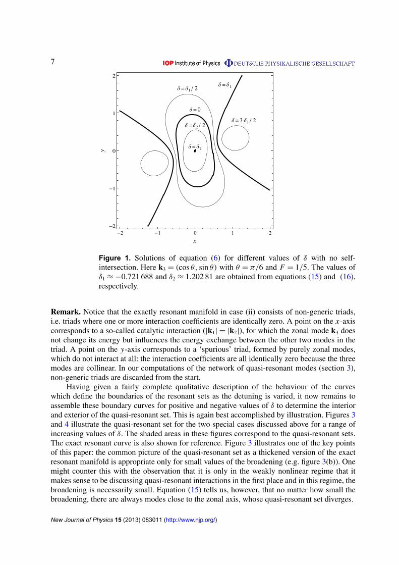
Figure 1. Solutions of equation (6) for different values of δ with no self-intersection. Here k3 = (cos θ, sin θ) with θ = π/6 and F = 1/5. The values ofδ1 ≈ −0.721 688 and δ2 ≈ 1.202 81 are obtained from equations (15) and (16),respectively.

Remark. Notice that the exactly resonant manifold in case (ii) consists of non-generic triads,i.e. triads where one or more interaction coefficients are identically zero. A point on the x-axiscorresponds to a so-called catalytic interaction (|k1| = |k2|), for which the zonal mode k3 doesnot change its energy but influences the energy exchange between the other two modes in thetriad. A point on the y-axis corresponds to a ‘spurious’ triad, formed by purely zonal modes,which do not interact at all: the interaction coefficients are all identically zero because the threemodes are collinear. In our computations of the network of quasi-resonant modes (section 3),non-generic triads are discarded from the start.

Having given a fairly complete qualitative description of the behaviour of the curveswhich define the boundaries of the resonant sets as the detuning is varied, it now remains toassemble these boundary curves for positive and negative values of δ to determine the interiorand exterior of the quasi-resonant set. This is again best accomplished by illustration. Figures 3and 4 illustrate the quasi-resonant set for the two special cases discussed above for a range ofincreasing values of δ. The shaded areas in these figures correspond to the quasi-resonant sets.The exact resonant curve is also shown for reference. Figure 3 illustrates one of the key pointsof this paper: the common picture of the quasi-resonant set as a thickened version of the exactresonant manifold is appropriate only for small values of the broadening (e.g. figure 3(b)). Onemight counter this with the observation that it is only in the weakly nonlinear regime that itmakes sense to be discussing quasi-resonant interactions in the first place and in this regime, thebroadening is necessarily small. Equation (15) tells us, however, that no matter how small thebroadening, there are always modes close to the zonal axis, whose quasi-resonant set diverges.

New Journal of Physics 15 (2013) 083011 (http://www.njp.org/)

8

2 2

2

0 12 1

2 1 0 1 22

1

0

1

2

x

y

Figure 2. Solutions of equation (6) for different values of δ which self-intersectat δ = δ2. Here k3 = (cos θ, sin θ) with θ = 3π/7 and F = 1/5. The values ofδ1 ≈ −0.185 434 and δ2 ≈ 0.309 057 are obtained from equations (15) and (16),respectively.

3. Structure of the network of quasi-resonant modes

In a turbulent system many modes are excited. The fact that a mode can be a member of morethan one quasi-resonant set leads to overlap between sets. This allows modes to join togetherto form a network of quasi-resonant clusters analogous to the exactly resonant clusters whichhave been extensively studied in the literature to date. In this section we study the structure ofthis quasi-resonant network as the typical amount of broadening, δ, in the system is varied. Weconsider a finite system of size 2π × 2π and truncate the wavenumber space such that there areM modes in the kx and ky directions, M2 modes in all. The spacing between modes is 2π/M .The quasi-resonant clusters were obtained by an exhaustive numerical search speeded up byincorporating symmetries of the triads. As explained in the remark below equation (18), wehave eliminated from our list of triads the so-called non-generic triads, i.e. the triads for whichone or more interaction coefficients are zero. This includes triads formed out of collinear modesand triads where any two wave-vectors have the same modulus.

We first measure the total number of clusters normalized by the maximum number ofpossible isolated clusters which is approximately M4/3. This is shown as a function of δ forseveral different system sizes, M , in figure 5. For each system size, as δ increases, the totalnumber of clusters first increases, then reaches a maximum at a particular value of δ, which weshall denote by δ∗, and then decreases. The value, δ∗, at which the maximum occurs decreases

New Journal of Physics 15 (2013) 083011 (http://www.njp.org/)

9

0

2 1 0 1 22

1

0

1

2

x

y

(a) δ = 0

0.5

2 1 0 1 22

1

0

1

2

xy

(b) δ = 1/2

1

2 1 0 1 22

1

0

1

2

x

y

(c) δ = 1

2

2 1 0 1 22

1

0

1

2

x

y

(d) δ = 2

3

2 1 0 1 22

1

0

1

2

x

y

(e) δ = 3

4

2 1 0 1 22

1

0

1

2

x

y

(f) δ = 4

Figure 3. Shaded regions correspond to the resonant set defined by equation (4)with k3 = (1, 0), F = 0 and β = 1 for different values of δ. The exactly resonantmanifold is the red solid line. (a) δ = 0, (b) δ = 1/2, (c) δ = 1, (d) δ = 2, (e)δ = 3 and (f) δ = 4.

as the system size, M , is increased. In order to understand these results one must realize thatfor the CHM dispersion relation, the number of exactly resonant clusters which live on the gridof discrete wavevectors is rather small with most discrete triads necessarily exhibiting a smallamount of detuning enforced by the geometry. The initial growth in the number of clusters isexplained by the addition of isolated triads to the list of quasi-resonant clusters as the broadeninggrows large enough to incorporate the geometrical detuning generated by the grid. While onewould expect this rate of increase to slow down as clusters start joining to form larger clusters,the attainment of a maximum and subsequent decrease in the total number of clusters becomesmuch easier to understand when we measure the size of largest cluster, ρ, which is simply thenumber of modes in the largest cluster normalized by the system size, M2. This is shown infigure 6. We see that as δ approaches δ∗ the largest cluster quickly makes a transition fromincluding a negligible fraction of the total number of modes in the system to including almostall of them. Thus the network of quasi-resonant modes undergoes a percolation transition atδ = δ∗. While the results shown in figures 5 and 6 were obtained for β = F = 1, we checkedthat the results are not very sensitive to this choice.

The decrease of the percolation threshold, δ∗, as the system size, M , increases is clearlydue to the fact that as M increases, the spacing between discrete modes decreases. The amount

New Journal of Physics 15 (2013) 083011 (http://www.njp.org/)

10

0

2 1 0 1 22

1

0

1

2

x

y

(a) δ = 0

0.1

2 1 0 1 22

1

0

1

2

xy

(b) δ = 1/10

0.5

2 1 0 1 22

1

0

1

2

x

y

(c) δ = 1/2

Figure 4. Shaded regions correspond to the resonant set defined by equation (4)with k3 = (0, 1), F = 0 and β = 1 for different values of δ. The exactlyresonant manifold is the red solid line and corresponds to the two axes in thiscase. As explained in the remark below equation (18), this exactly resonantmanifold consists of non-generic triads, i.e. triads where one or more interactioncoefficients are identically zero. The case F = 0 is chosen for simplicity only:for F > 0, the resonant sets have the same qualitative shape as in the case F = 0.(a) δ = 0, (b) δ = 1/10 and (c) δ = 1/2.

10−10

10−8

10−6

10−4

10−2

0

0.02

0.04

0.06

0.08

0.1

0.12

0.14

0.16

δ

Nor

mal

ized

Tot

al N

umbe

r of

Clu

ster

s

M = 16M = 32M = 64M = 128M = 256

Figure 5. The normalized total number of clusters, N , plotted as a function of δfor different system sizes, M . Here, we have fixed F = β = 1.

of broadening required to overcome the geometrical detuning is therefore smaller and henceclusters can form more easily. We would like to quantify this decrease. We have already learnedthat the area of the quasi-resonant set of any particular mode, k, diverges at a finite value of

New Journal of Physics 15 (2013) 083011 (http://www.njp.org/)

11

0

0.2

0.4

0.6

0.8

1

1.2

1.4

10-13 10-12 10-11 10-10 10-9 10-8 10-7 10-6 10-5

ρ

δ

M=100M=200M=500

M=1000

0

0.2

0.4

0.6

0.8

1

0 2 4 6 8 10

ρ

δ M3

Figure 6. The density of the largest cluster, ρ, as a function of resonancebroadening δ for different system sizes, M . Here we have fixed F = β = 1. Thepercolation threshold, δ∗, decreases as a function of system size. The inset showsthe same data plotted as a function of δ M3. The solid line is a fit of equation (21)to the data.

δ = ω(k) as indicated in equation (15). It seems plausible that as soon as the broadening issufficiently large to allow any mode in the system to have a divergent quasi-resonant set, thenthe largest cluster must be of the size of the system. Thus one might estimate

δ∗ ≈ mink

|ω(k)|. (19)

If this argument was correct, equation (2) tells us that for large systems we should see thescaling, δ∗ ∼ M−2. A numerical measurement of the scaling of δ∗ scales with system size, M ,for a range of values of F , is plotted in figure 7 and gives a different answer. For each value ofF , the curve converges to the straight line indicated by the scaling

δ∗ ∼ M−σ1 (20)

with exponent σ1 = 3.00 with a 95% confidence intervals of (2.97, 3.03), which was obtainedby bias-corrected bootstrapping. The connected component therefore forms much more easilythan the above naive argument above would suggest. The origin of this M−3 scaling can betraced to the fact that zonal modes require very little detuning in order to interact with high kalmost meridional modes. Take F = 0 for simplicity, although the following argument works forany F > 0. Let us consider the largest-scale zonal mode in the system, k = (0, 1).We recall thatthe exactly resonant manifold xy = 0 of this zonal mode, figure 4(a), gives rise to non-generictriads which do not interact efficiently and therefore must be discarded. So we ask what is theminimum value of the detuning so that the quasiresonant set of the mode k = (0, 1) containssome new modes. From figure 4(b) it is clear that the first new mode to join the quasi-resonantset will be k1 = (M, 0), corresponding to x = M , y = −1/2. By substituting these values of

New Journal of Physics 15 (2013) 083011 (http://www.njp.org/)

12

102

103

10−9

10−8

10−7

10−6

M

δ*

F = 100

F = 101

F = 102

F = 103

F = 104

Figure 7. Percolation threshold, δ∗, plotted against system size and for differentvalues of F . Here, we have fixed β = 1. For large system sizes, δ∗ exhibits thescaling δ∗ ∼ M−σ1 , where we measure σ1 = 3.00(2.97, 3.03). The brackets showthe 95% confidence interval.

x, y into equation (18), we obtain[(M2 +

1

4

)2

+1

2

(M2

−1

4

)+

1

16

]δ∗ = M.

For large M , this has solution δ∗ ∼ M−3, in agreement with figure 7 and the inset of figure 6.This suggests that the percolation transition is driven by interactions between large-scale zonalmodes and small scale meridional modes. This is consistent with the known scale-non-localityof wave turbulence in the CHM equation (see [33] and the references therein) and providesfurther evidence, albeit circumstantial, that the percolation transition is associated with the onsetof turbulence in the CHM model.

In order to further illustrate this point, we can ask which modes have the greatest or leasttendency to become part of a quasi-resonant cluster. This is done in figure 8, where we havecoloured each mode according to the minimal amount of resonance broadening required forthis mode to join a cluster of any size. Blue modes become active very easily whereas redmodes are resilient to becoming part of any cluster. Rather than appearing homogeneous andrandom, we see the appearance of definite structure. We see a circular region containing modeswith a strong propensity to join clusters including a narrow large-scale region of zonal modesaccumulating near the kx = 0 axis with very low interaction thresholds as expected from thediscussion above. We also remark upon the group of large-scale meridional scales reluctant toform any quasi-resonant connections. The relative reluctance of large-scale meridional modesto exchange energy has already been remarked upon in the literature and suggested as an

New Journal of Physics 15 (2013) 083011 (http://www.njp.org/)

13

kx

k y

50 100 150 200 250

−250

−200

−150

−100

−50

0

50

100

150

200

250 −10

−9.5

−9

−8.5

−8

−7.5

−7

−6.5

−6

−5.5

−5

log10

(δ )

Figure 8. Colour map in k-space showing the smallest value of broadeningrequired for each mode to become a member of a cluster of any size. The darkerregions are resilient to becoming members of clusters in the sense that largevalues of broadening are required. Lighter regions join clusters easily.

explanation of the inherent anisotropy of Rossby wave turbulence. For example in [34], a wave-turbulence boundary was computed by comparing the CHM dispersion relation to the inverseof the eddy-turnover time. It is then argued that inside this region Rossby waves dominate, butwith a frequency incommensurate with that of the surrounding turbulence so that energy cannotpenetrate into this region. The boundary thus obtained seems similar in position and shape to thedark region in figure 8. This anisotropic energy distribution at large scales has been documentedin numerical simulations of Rossby wave turbulence (see [35] and the references therein). It issomewhat surprising to see it emerging again here from purely kinematic considerations.

Finally we might ask whether the density of the giant cluster illustrated in figure 6 showsthe generic profile for a second order phase transition,

ρ(δ)=

{0 δ 6 δ∗

c (δ− δ∗)z δ > δ∗,

(21)

and, if so, what is the exponent z. Notice that the system size M has been absorbed afterappropriate rescalings of δ and δ∗ by the factor M3. Equation (21) contains three adjustableparameters, δ∗, c and z, which makes it difficult to unambiguously determine the exponent z. Aspointed out in [36], if equation (21) holds, then

ρ

(dρ

dδ

)−1

=1

z(δ− δ∗) (22)

for δ > δ∗. Plotting this quantity against δ produces an easier fitting problem because theamplitude c cancels out, the fitting becomes linear and the value of δ∗ corresponds to the point at

New Journal of Physics 15 (2013) 083011 (http://www.njp.org/)

14

0

0.5

1

1.5

2

2.5

3

3.5

4

0 0.5 1 1.5 2 2.5 3 3.5 4

ρ (d

ρ/dδ

)-1

δ

Numerical dataLinear fit

Figure 9. Fitting the data in figure 6 to a standard phase transition profile. Theleft-hand side (LHS) of equation (21) is plotted as a function of δ. The fit (solidline) is taken over the range [δ∗ : 2] with δ∗ = 0.815. It has slope 2.03. whichsuggests a value of z ≈

12 .

which the fitted line crosses zero. The values of dρdδ would ideally be obtained independently from

the values for ρ. In our case, this was not possible so we obtained them by locally interpolatingthe measured values of ρ using Mathematica and differentiating the result. The outcome ofthis analysis is shown in figure 9. We can see that a case can be made for a linear fit in theneighbourhood of δ∗. Taking δ∗ = 0.815 (the point at which the straight line fit obviously startsto fail), and fitting the data over the range [δ∗ : 2] gives the fit shown in the figure. The slopegives a value of z ≈

12 . This is standard Landau value for the mean field theory of a second

order phase transition of a scalar field. These results, while suggestive, are far from definitive.A more detailed numerical study in the vicinity of δ∗ will be required before we can start puttingestimates of uncertainty on these values. For the purposes of comparison, equation (21) with thebest fit values of the parameters, is plotted with the original data in the inset of figure 6 (solidline).

4. Conclusions and outlook

To conclude, we have presented a kinematic analysis of the properties of quasi-resonant triadsin the CHM equation. We described the analytic form of the quasi-resonant set defined bythe quasi-resonance conditions, equation (4), as a function of the resonance broadening, δ. Wefound that they have non-trivial geometric shape and are not well described as simply thickenedversions of the exact resonant manifold as is commonly assumed. In particular, we found thatthe quasi-resonant set becomes unbounded above a critical value of δ and that this can occurfor arbitrarily small values of δ as we consider modes approaching the zonal axis. We thenconducted an in-depth numerical study of the structure of quasi-resonant clusters as a function

New Journal of Physics 15 (2013) 083011 (http://www.njp.org/)

15

of δ and identified a percolation transition as δ is increased. At the transition, a large cluster isformed which contains a finite fraction of all the modes in the system. For a system containingM2 modes, the value of the percolation threshold decreases as M−3. This scaling results from theease with which large-scale zonal modes interact with small scale meridional modes, a reflectionof the non-locality of Rossby wave turbulence.

We speculate that the percolation transition corresponds dynamically to the transitionfrom mesoscopic to classical wave turbulence. The fact that a percolation transition exists isconsistent with earlier work on capillary waves [26]. In fact, we believe that this transitionis not a special feature of the CHM dispersion relation and is generic [37]. Furthermore ourresults provide circumstantial support for the sandpile picture of mesoscopic wave turbulencesuggested in [30] since a small change in resonance broadening in the vicinity of δ∗ cantrigger a transition from a state which cannot support an energy cascade to one which can.In order to better understand these issues, we believe that it is important to move beyond thekinematic picture of resonance broadening and attempt to devise methods of studying theseeffects dynamically.

Acknowledgments

CC acknowledges the support of the EPSRC grant EP/H051295/1 and the Fields Institute atthe University of Toronto, MDB acknowledges support from University College Dublin, SeedFunding Projects SF564 and SF652.

Appendix. Characterization of the quasi-resonant set for a single triad

This appendix provides additional technical details related to the properties of the curve (11)describing the boundary of the resonant set. After shifting the origin to the centre of symmetryof the curve using the variable x and y defined by (12) and rescaling δ to remove β, the curvewe wish to study is

−p

k2 + F+

x + p/2

(x + p/2)2 + (y + q/2)2 + F−

x − p/2

(x − p/2)2 + (y − q/2)2 + F= δ. (A.1)

Gathering these terms together with a common denominator we obtain the quartic curve

c(x, y)= a1 + a2(x2 + y2)2 + a3x2 + a4 y2

− a5xy = 0, (A.2)

where the coefficients are given by

a1 =1

16 (k2 + 4F)[3k2 p − (k2 + F)(k2 + 4F) δ],

a2 = − p − (k2 + F) δ,

a3 = −12 [p(p2 + 3q2 + 6F)− (k2 + F)(p2

− q2− 4F) δ],

a4 =12 [p(p2 + 3q2

− 2F)− (k2 + F)(p2− q2 + 4F) δ],

a5 = 2q[q2 + F − p(k2 + F) δ].

Upon introduction of the variables u = x2, v = y2 and w = xy, it becomes clear thatequation (A.1) corresponds to the intersection of the two quadratic surfaces given by

New Journal of Physics 15 (2013) 083011 (http://www.njp.org/)

16

equations (14) in the main text. We have performed a full analysis of the properties of theintersection of these curves for general values of the parameters p, q, F and δ but, as mentionedin the main text, this exercise is not very illuminating. The following qualitative features give agood picture of the general behaviour of these curves:

(i) The curve typically exists only for a finite range of δ.This is evident from studying equation (A.1) as δ → ±∞. The LHS can only diverge ifone of the denominators diverges. This is impossible if F > 0. Hence if F > 0, solutionsto equation (A.1) must cease to exist if δ gets too large by absolute value. In theexceptional case F = 0, solutions indeed exist for all values of δ and become localizedin the neighbourhood of ±(p/2, q/2) as δ → ±∞.

(ii) The curve is bounded except at single critical value of δ.Examining equation (14), it is clear that since u and v are both positive, it is generallynot possible to balance the quadratic terms if u2 + v2

→ ∞. Hence the curve, if it exists isbounded. The single exception to this occurs when the coefficient of the quadratic termsvanishes. The curve may therefore diverge at the single critical value of detuning given byequation (15) in the main text

δ = δ1 ≡ −p

k2 + F.

Note that this corresponds to δ = ω(k3). At δ = δ1, some algebra shows that the curve isgiven by the hyperbola

x2 + 2q

pxy − y2

=14 (k

2 + F). (A.3)

(iii) The curve may self-intersect only at a single critical value δ.From equation (14), self-intersection is only possible if the curve passes through (0, 0) inthe (u, v) plane. This can only happen if the coefficient a1 = 0. Thus we identify the secondcritical value of δ given by equation (16) of the main text:

δ = δ2 =3k2 p

(k2 + F)(k2 + 4F).

Note that a1 = 0 does not necessarily mean the curve self-intersects. It is possible that atδ = δ2, the curve reduces to a single point. To probe what happens at δ = δ2, we considerthe surface z = c(x, y) defined by equation (A.2) when δ = δ2 in the neighbourhood of theorigin. Calculation of the partial derivatives indicate that this surface has a critical point atthe origin. After some tedious algebra, we find that the determinant of the matrix of secondderivatives is

1= −4(k2 + F)2(k4 + 4(q2

− 3p2)F)

k2 + 4F.

If1> 0 then the critical point at (0, 0) is a maximum or a minimum. The curve c(x, y)= 0is then an isolated point. On the other hand, if 1< 0 the critical point is a saddle and thecurve c(x, y)= 0 has a self-intersection at (0, 0). The condition for self-intersection istherefore

k4 + 4(q2− 3p2)F > 0. (A.4)

We note that for F = 0 we always have a self-intersection.

New Journal of Physics 15 (2013) 083011 (http://www.njp.org/)

17

These qualitative features of the boundary of the quasi-resonant set are illustratedgraphically in figures 1 and 2 in the main text. These figures are illustrative of the typicalbehaviour for general values of p, q and F .

References

[1] Whitham G B 1974 Linear and Nonlinear Waves (New York: Wiley)[2] Zakharov E V, Lvov S V and Falkovich G 1992 Kolmogorov Spectra of Turbulence (Berlin: Springer)[3] Graff K F 1991 Wave Motion in Elastic Solids (New York: Dover)[4] Horton W and Hasegawa A 1994 Quasi-two-dimensional dynamics of plasmas and fluids Chaos 4 227–51[5] Pedlosky J 1987 Geophysical Fluid Dynamics 2nd edn (New York: Springer) chapter 3[6] Sagdeev Z and Galeev A A 1969 Nonlinear Plasma Theory (New York: Benjamin)[7] Armstrong J A, Bloembergen N, Ducuing J and Pershan P S 1962 Interactions between light waves in a

nonlinear dielectric Phys. Rev. 127 1918–39[8] McComas C H and Bretherton F P 1977 Resonant interaction of oceanic internal waves J. Geophys. Res.

82 1397–412[9] Alex Craik D D 1988 Wave Interactions and Fluid Flows (Cambridge: Cambridge University Press)

[10] Lynch P and Houghton C 2004 Pulsation and precession of the resonant swinging spring Physica D 190 38–62[11] Bustamante M D and Kartashova E 2009 Effect of the dynamical phases on the nonlinear amplitudes’

evolution Europhys. Lett. 85 34002[12] Bustamante M D and Kartashova E 2011 Resonance clustering in wave turbulent regimes: integrable

dynamics Commun. Comput. Phys. 10 1211[13] Harris J, Bustamante M D and Connaughton C 2012 Externally forced triads of resonantly interacting waves:

Boundedness and integrability properties Commun. Nonlinear Sci. Numer. Simul. 17 4988–5006[14] Nazarenko S V 2011 Wave Turbulence (Lecture Notes in Physics vol 825) (Heidelberg: Springer)[15] Newell A C and Rumpf B 2011 Wave turbulence Ann. Rev. Fluid Mech. 43 59–78[16] Newell A C, Nazarenko S and Biven L 2001 Wave turbulence and intermittency Physica D 152–153 520–50[17] Bustamante M D and Hayat U 2013 Complete classification of discrete resonant Rossby/drift wave triads on

periodic domains Commun. Nonlinear Sci. Numer. Simul. 18 2402–19[18] Bustamante M D and Kartashova E 2009 Dynamics of nonlinear resonances in Hamiltonian systems

Europhys. Lett. 85 14004[19] Kartashova E and L’vov V S 2007 Model of intraseasonal oscillations in earth’s atmosphere Phys. Rev. Lett.

98 198501[20] L’vov V S, Pomyalov A, Procaccia I and Rudenko O 2009 Finite-dimensional turbulence of planetary waves

Phys. Rev. E 80 066319[21] Kartashova E 1998 Wave resonances in systems with discrete spectra Nonlinear Waves and Weak Turbulence

vol 182 (AMS Translations 2), ed V E Zakharov (Providence, RI: American Mathematical Society)pp 95–130

[22] Dyachenko A I, Korotkevich A O and Zakharov V E 2003 Decay of the monochromatic capillary wave J. Exp.Theor. Phys. Lett. 77 477–81

[23] Connaughton C, Nadiga B, Nazarenko S V and Quinn B E 2010 Modulational instability of Rossby and driftwaves and the generation of zonal jets J. Fluid Mech. 654 207–31

[24] Pushkarev A N 1999 On the kolmogorov and frozen turbulence in numerical simulation of capillary wavesEur. J. Mech. B 18 345–51

[25] Pushkarev A N and Zakharov V E 2000 Weak turbulence of capillary waves Physica D 135 98[26] Connaughton C, Nazarenko S V and Pushkarev A N 2001 Discreteness and quasi-resonances in weak

turbulence of capillary waves Phys. Rev. E 63 046306[27] Kartashova E 2009 Discrete wave turbulence Europhys. Lett. 87 44001

New Journal of Physics 15 (2013) 083011 (http://www.njp.org/)

18

[28] L’vov V S and Nazarenko S 2010 Discrete and mesoscopic regimes of finite-size wave turbulence Phys. Rev. E82 056322

[29] Zakharov V E, Korotkevich A O, Pushkarev A N and Dyachenko A I 2005 Mesoscopic wave turbulenceJ. Exp. Theor. Phys. Lett. 82 487–91

[30] Nazarenko S 2006 Sandpile behaviour in discrete water-wave turbulence J. Stat. Mech. Theor. E 2006 L02002[31] Lvov Y V, Nazarenko S and Pokorni B 2006 Discreteness and its effect on water-wave turbulence Physica D

218 24–35[32] Stauffer D and Aharony A 1994 Introduction To Percolation Theory revised 2nd edn (Philadelphia, PA: Taylor

and Francis) chapter 5, pp 89–113[33] Connaughton C, Nazarenko S V and Quinn B E 2011 Feedback of zonal flows on wave turbulence driven by

small-scale instability in the Charney–Hasegawa–Mima model Europhys. Lett. 96 25001[34] Vallis G K 2006 Atmospheric and Oceanic Fluid Dynamics (Cambridge: Cambridge University Press)[35] Huang H P, Galperin B and Sukoriansky S 2001 Anisotropic spectra in two-dimensional turbulence on the

surface of a rotating sphere Phys. Fluids 13 225–40[36] Connaughton C and Nazarenko S V 2004 Warm cascades and anomalous scaling in a diffusion model of

turbulence Phys. Rev. Lett. 92 044501[37] Harris J, Bustamante M D and Connaughton C 2013 Kinematics of quasi-resonances in 3-wave systems with

isotropic scale-invariant dispersion, in preparation

New Journal of Physics 15 (2013) 083011 (http://www.njp.org/)