Perfect simulation with exponential tails on the running time

Perfect Simulation With Exponential Tailson the Running Time

Mark Huber*Department of Mathematics and ISDS, Duke University, Durham, NC 27713;

e-mail: [email protected]

Received 15 September 2006; accepted 14 May 2007; received in final form 15 June 2007Published online 2 April 2008 in Wiley InterScience (www.interscience.wiley.com).DOI 10.1002/rsa.20212

ABSTRACT: Monte Carlo algorithms typically need to generate random variates from a probabilitydistribution described by an unnormalized density or probability mass function. Perfect simulationalgorithms generate random variates exactly from these distributions, but have a running time T thatis itself an unbounded random variable. This article shows that commonly used protocols for creatingperfect simulation algorithms, such as Coupling From the Past can be used in such a fashion thatthe running time is unlikely to be very much larger than the expected running time. © 2008 WileyPeriodicals, Inc. Random Struct. Alg., 33, 29–43, 2008

Keywords: Monte Carlo; perfect simulation; coupling from the past; noninterruptible algorithms

1. MONTE CARLO METHODS

Perfect simulation algorithms require an unbounded random amount of time T to generaterandom variates from distributions. This article looks into a natural question about thesealgorithms, namely, how likely is T to be very much larger than its expected value?

The basic problem of Monte Carlo algorithms is the following. Given a target distributionπ over a measurable state space (�, F), generate random variates drawn from this distrib-ution. Monte Carlo methods are used in statistics to estimate exact p-values [1], in physicsto estimate partition functions [12], in computer science for approximation algorithms for#P complete problems [11], and in a variety of other applications (see [6] for an overview).

Correspondence to: M. Huber*Supported by NSF CAREER (DMS-05-48153).© 2008 Wiley Periodicals, Inc.

29

30 HUBER

Typically the distribution is given in terms of an unnormalized density or probability massfunction:

π(dx) = [f (x)dx]/Z , or π(x) = w(x)/Z . (1.1)

Often it is an #P complete problem to compute Z exactly.The classical approach to this problem is to use Monte Carlo Markov chain methods.

Using a technique such as Gibbs sampling or Metropolis-Hastings, build a Markov chainwhose stationary distribution matches π . Then, starting from an arbitrary state, run theMarkov chain forward until the distribution of the state is close to stationary.

Unfortunately, it is usually very difficult to ascertain how long a Markov chain must berun before the state is close to stationary. Heuristic tests such as autocorrelation can alertthe user when the state is far away from stationarity, but cannot guarantee that the samplegenerated has a distribution close to the target.

Coupling from the past (CFTP) [13] was the first widely used perfect simulationalgorithm. The advantages of a perfect simulation algorithm are twofold.

1. Random variates come exactly from the desired distribution π (they are exactsimulation methods.)

2. They are true algorithms where number of steps that need to be taken variesdynamically with the problem.

There are situations where an analysis of the mixing time of the Markov chain is possible([2,10]). These results are usually of the following form. Define the total variation distancebetween distributions ν1 and ν2 on (�, F):

dTV (ν1, ν2) := supA∈F

|ν1(A) − ν2(A)|. (1.2)

Consider a Markov chain with stationary distribution π , and let x0 ∈ �, and pt(x0) be thedistribution of the state of the Markov chain after t steps given that the state started in x0.Note that dTV (pt(x0), π) is a decreasing function of time. Set

τ(x0, ε) = inf{t : dTV (pt(x0), π) ≤ ε}. (1.3)

Then τ(x0, ε) is the mixing time of the chain started at x0. Taking the supremum over allx0 ∈ � gives the mixing time of the chain τ(ε).

The chain is rapidly mixing if τ(ε) = p1(n) + p2(n) ln(ε−1), where n is a measure ofproblem input size and p1 and p2 are O(nd) for some d.

When a perfect simulation algorithm with bounded expected running time and a rapidlymixing Markov chain both exist for a problem, it is usually better to run the perfect simulationmethod. For this, consider a Markov chain where the mixing time for a fixed ε is shown to beless than or equal to p(n). Then p(n) steps must be taken for each random variate generatedin order to guarantee that the chain has mixed. That is, the algorithm to approximatelygenerate variates will be �(p(n)). Unless the user is willing to reanalyze the mixing timeargument for the specific problem at hand, the full p(n) steps must be taken every singletime.

On the other hand, perfect sampling methods are algorithms whose running time Thas a distribution that varies depending on the problem at hand. Suppose that b(n) is anupper bound on the expected running time of the algorithm for all problem instances. Then

Random Structures and Algorithms DOI 10.1002/rsa

EXPONENTIAL TAILS FOR PERFECT SIMULATION 31

for specific problems the algorithm could take much less time then b(n). This gives thealgorithm an O(b(n)) expected running time.

This is well-known in studying other algorithms: bubble sort is well-known to be anO(n2) sorting algorithm but can take �(n) time on inputs that are close to being sorted.But with approximate variate generation for Markov chains with known mixing time, thealgorithms created are always �(p(n)) rather than O(p(n)). This can give a large speedadvantage for perfect simulation methods.

The expected value of the running time for a perfect sampling algorithm can be verysmall. However, this hides an important question: even if the expected run time is small,what about the tail of the distribution? This is the question addressed in this article, whereit is shown that for several common perfect simulation methods (including basic CFTP), itis possible to run these algorithms in such a manner that the probability that the runningtime is much greater than the expected time declines faster than any polynomial.

Theorem 1.1. Consider an interruptible perfect simulation algorithm or Coupling Fromthe Past (CFTP) with running time T. If E[T ] < ∞ and is known, it is possible to run thesealgorithms so that

P(T > kE[T ]) ≤ 2 exp(−k(ln 2)/4) (1.4)

independent of the problem.If the mean of T is unknown, it is possible to run these algorithms in such a fashion so

that for k ≥ 2,P(T > kE[T ]) ≤ 4 exp(−0.186kln 2/ ln 3) (1.5)

independent of the problem.

Equation (1.4) follows from Lemma 2.1 in Section 2, and Lemma 5.1 in Section 5. Note(1.5) provides a slightly weaker bound on the tail of T , although both bounds decline fasterthan any polynomial in k. It is to be expected that (1.5) is weaker as the mean E[T ] isunknown in this case. The method for proving (1.5) is shown in Section 4 for interruptiblemethods and Section 5 for CFTP, and follows from Lemmas 4.1 and 5.3.

The next section defines perfect sampling and interruptibility, and develops the basicmethods for interruptible algorithms. Section 3 analyzes the running time of interruptiblemethods using a known procedure, the doubling method. Section 4 develops a new procedureby expanding upon the doubling method that has much smaller tails on the running time.Section 5 shows how to apply these analyses and methods to Coupling From the Past.

2. INTERRUPTIBLE PERFECT SAMPLING

Perfect sampling protocols such as Coupling From the Past [13] (and variants), cycle pop-ping [14], FMMR [5], and the Randomness Recycler [4] all can be used to design algorithmsto generate samples from a particular target distribution. The downside of these algorithms isthat the running time of the procedure is itself a random variable that can be arbitrarily large.

Definition. For a target distribution π , a perfect sampling algorithm

1. outputs random variates whose distribution is exactly π ,2. has a running time T such that P(T > t) > 0 for any positive t.


32 HUBER

The second part of the definition is needed to distinguish perfect sampling algorithmsfrom algorithms that compute the normalizing constant explicitly in a deterministic fashion.Dynamic programming is an example of a protocol for creating algorithms that falls in thiscategory, and such algorithms are not typically referred to as perfect sampling algorithms.

Example 1. A perfect simulation algorithm for a geometric random variable withparameter p.

GEOInput: p, Output: X1) Let X ← 01) Repeat2) Choose U ← Unif[0, 1], Let X ← X + 13) Until U ≤ p

As with GEO, many Monte Carlo algorithms are iterative in nature, with the time neededfor one step being dominated by the generation of a pseudorandom number drawn uniformlyfrom [0, 1]. Therefore it is customary to measure the running time of these algorithms by thenumber of uniforms that they utilize. In the example above, if T is the number of uniformsused, then X = T .

Definition. A perfect sampling algorithm with output X and running time T is interruptibleif X has distribution π when conditioned on T .

The above example is a noninterruptible algorithm, since X conditioned on T equals T .A user running the algorithm GEO must commit to running the algorithm to completionwith probability 1, otherwise bias will be introduced into the sample. For instance, if a userbegins a run of a noninterruptible algorithm knowing that they only have time to generate onemillion uniforms, then the output will not be from π , but instead comes from X conditionedon T ≤ 106. In the above example it is easy to determine how this changes the distributionbut in more complex situations this is rarely possible.

By contrast, an interruptible perfect sampling algorithm can be aborted and restartedin the middle of a run without altering the distribution of the output. The algorithmTIMED_ALG explicitly aborts after a time limit.

TIMED_ALG: Interruptible perfect sampling with time limitInput: t1) Run interruptible perfect sampler for t time steps or until it finishes2) If the algorithm finished, output the result3) Else output ⊥

Let m(T) denote the smallest median of the random variable T (note that while the medianmight not be unique as T is integral, the set of medians will have a smallest element.) Whenthe input to TIMED_ALG is t = m(T), the probability that ⊥ is output is at most 1/2.When m(T) is polynomial in the problem input size, Dyer and Greenhill [3] called such analgorithm a “strong perfect sampler.”

The following algorithm breaks the interruptible algorithm into blocks of fixed length,as illustrated in Fig. 1.



Fig. 1. Blocks of fixed length.

Interruptible perfect sampling with fixed length blocksInput: t, Output: Y1) Repeat2) Let Y be the result of TIMED_ALG(t)3) Until Y �= ⊥

Lemma 2.1. Let T be the running time of the original interruptible perfect samplingalgorithm. Suppose m(T) is known, and let TK be the running time of the interruptibleperfect sampling with t = m(T). Then

E[TK ] ≤ 2m(T) and (∀k ≥ 0)(P(TK > k · m(T)) ≤ 2(1/2)k). (2.1)

If T has a known finite expectation then the running time of fixed length interruptible perfectsampling with t = 2E[T ] satisfies

E[TK ] ≤ 4E[T ] and (∀k ≥ 0)(P(TK > kE[T ]) ≤ 2(1/2)k/2). (2.2)

Proof. The number of times through the repeat loop in the algorithm is a geometric randomvariable with parameter at least 1/2, and each run through the loop takes m(T) time. Hencethe expected number of runs through the loop is at most 2, and P(TK > km(T)) ≤ (1/2)k ≤2(1/2)k . If T has finite expectation, then m(T) ≤ 2E[T ] by Markov’s inequality, and thebound is (1/2)k/2 ≤ 2(1/2)k/2 and (2.2) follows.

3. INTERRUPTIBLE PERFECT SAMPLING WITH UNKNOWN RUNNING TIME

The previous section dealt with the situation where the median or expectation of the runningtime T was known before starting the algorithm. Unfortunately, this is rarely the case.In their original paper on Coupling From the Past, Propp and Wilson [13] suggested away around this problem: doubling the amount of time given to each block, as shownin Fig. 2.

Their technique can be applied to interruptible perfect simulation as follows.

Fig. 2. Doubling block length.


34 HUBER

Doubling algorithm for interruptible perfect samplingOutput: Y1) Let t ← 12) Repeat3) Let t ← 2t4) Let Y be the result of TIMED_ALG(t)5) Until Y �= ⊥

The expected running time for the doubling algorithm will be the same order as the(3/4)-quantile of T . When T has finite expectation, the doubling algorithm has expectedrunning time of the same order as E[T ] and the tail declines faster than any polynomial, butnot exponentially fast.

Lemma 3.1. Let T be the running time of the original interruptible perfect samplingalgorithm, and TD be the running time of the doubling algorithm for interruptible perfectsampling. Let s(T) be the smallest (3/4)-quantile of T , so that P(T ≥ s(T)) ≥ 1/4. Then

E[TD] ≤ 3s(T) and (∀k > 0)(P(TD > k · s(T)) ≤ 4/k2). (3.1)

If T has finite expectation then

E[TD] ≤ 3E[T ] and (∀k ≥ 3)(P(TD > kE[T ]) ≤ 0.242/k0.721 ln k−2.09 (3.2)

Proof. Let k ≥ 2, and suppose T > k · s(T). Then there must be at least one block that isof size between s(T) and 2s(T) that returned ⊥. In fact, because the block size is doublingat each step, there will be log2 k blocks of size at least s(T). The probability that any oneof these blocks returns ⊥ is at most 1/4, therefore the probability that all these blocks return⊥ is at most

(1/4)log2 k ≤ (1/4)(log2 k)−1 = 4/k2, (3.3)

so P(TD > k · s(T)) ≤ 4/k2. For k < 2, 4/k2 > 1 and the bound also holds.It remains to bound E[TD]. Since TD is a nonnegative random variable,

E[TD] =∫ ∞

0t dPTD(t)

≤∞∑

k=1

k · s(T)P((k − 1)s(T) < TD ≤ k · s(T))

= s(T)

[ ∞∑k=0

P(TD > k · s(T))

]

≤ s(T)

[P(TD > 0) +

∞∑k=1

(1/4)log2 k]

≤ s(T)[1 + (1/4)0 + 2(1/4)1 + 4(1/4)2 + . . .

] = 3s(T).

Now suppose that E[T ] < ∞. Markov’s inequality provides a means to obtain a strongerupper bound. Fix k ≥ 2 and let t = kE[T ]. Then for T > t, the last run between t − 2log2 t

and t has to fail, and the previous block as well. Let �1 := t −2log2 t and �2 := (1/2)2log2 t



denote the lengths of these two blocks. Block size doubles at each step, and so the lengthsof all the other blocks combined is exactly �2 − 1. Hence �1 + �2 + �2 − 1 = t. So either�1 ≥ t/3 or �2 ≥ t/3.

Hence there is a sequence of blocks of length at least t/3, t/6, t/12, . . .. By Markov’sinequality, a block of length t/a has probability at most E[T ]a/t = a/k of returning ⊥. So,the probability that all of the blocks return ⊥ is at most

f (k) = 3

k· 6

k· · · 3.2log2(k/3)

k. (3.4)

Note for integer i, when k = 3 · 2i, f (k) = 2−(i2+i)/2, and ln f (k) = −0.5(ln 2)(i2 +i). Since f (k) decreases in k, for all k: ln f (k) ≤ −0.5(ln 2)((log2 k/6)2 + log2 k/6), soln f (k) ≤ 0.5 ln 6−0.5(ln 6)2/ ln 2+ ln k[− ln k/(2 ln 2)+ ln 6/ ln 2−0.5]. Exponentiatingand bounding the constants yields f (k) ≤ 0.242/k0.721 ln k−2.09, giving the desired upperbound on P(TD > kE[T ]).

Bound E[TD] by considering P(TD > t). As above, TD > t implies that there is a blockof size at least t/3. The probability that this block fails is P(T > t/3), so:

∞∑t=0

P(TD > t) ≤∞∑

t=0

P(T > t/3) = 3E[T ]. (3.5)

Remark. The most important property of the doubling method is that even if T does nothave finite expectation, the doubling procedure will.

Remark. In Lemma 3.1, the (3/4)-quantile is utilized. In fact, any α-quantile could beused where α ∈ (1/2, 1) to achieve similar results. The closer α is to 1, the greater thepolynomial decrease for the tail.

4. TRIPLING METHOD FOR INTERRUPTIBLE PERFECT SAMPLING

In the previous section, the doubling method was described for interruptible perfect sam-pling. The analysis shows that when T has finite expectation, the tails decline exponentiallyat a rate of order (log k)2. For most applications, the simplicity of the doubling methodcombined with this dropoff in running time will be sufficient.

It is possible to do better. In this section a new method is described that has expectedrunning time that is of the order of α-quantiles for any α. Moreover, the tail of T declinesexponentially at rate of order kln 2/ ln 3. The cost is that the algorithm is somewhat morecomplex.

As in the previous section TIMED_ALG(t) will denote the interruptible algorithmwhich aborts and returns ⊥ if the running time is greater than t. The goal is to divide theallotted time into three pieces. Two of these pieces are recursive copies of the original, andthe last piece is just a run of TIMED_ALG. Because of the division by 3, this algorithm isnamed 3_REC.


36 HUBER

3_RECInput: t (where t = 3d for some integer d) Output: Y1) If t = 12) Let Y ← TIMED_ALG(1)

3) Else4) Let Y ← 3_REC(t/3)

5) If Y = ⊥6) Let Y ← 3_REC(t/3)

7) If Y = ⊥8) Let Y ← TIMED_ALG(t/3)

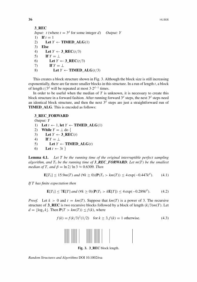
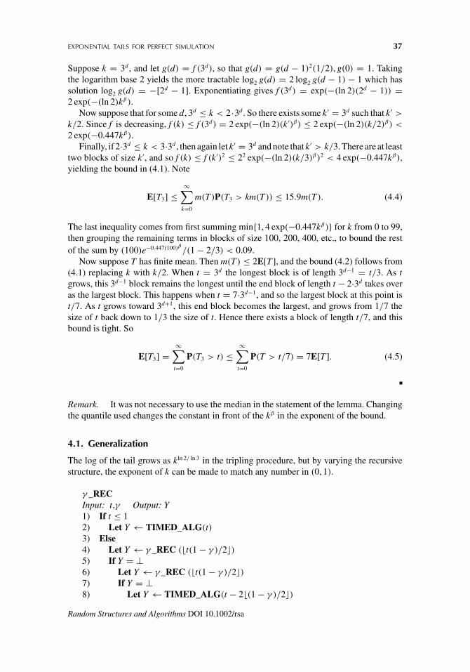
This creates a block structure shown in Fig. 3. Although the block size is still increasingexponentially, there are far more smaller blocks in this structure. In a run of length t, a blockof length t/3d will be repeated at most 3·2d−1 times.

In order to be useful when the median of T is unknown, it is necessary to create thisblock structure in a forward fashion. After running forward 3d steps, the next 3d steps needan identical block structure, and then the next 3d steps are just a straightforward run ofTIMED_ALG. This is encoded as follows:

3_REC_FORWARDOutput: Y1) Let t ← 1, let Y ← TIMED_ALG(1)

2) While Y = ⊥ do {3) Let Y ← 3_REC(t)4) If Y = ⊥5) Let Y ← TIMED_ALG(t)6) Let t ← 3t }

Lemma 4.1. Let T be the running time of the original interruptible perfect samplingalgorithm, and T3 be the running time of 3_REC_FORWARD. Let m(T) be the smallestmedian of T, and β = ln 2/ ln 3 ≈ 0.6309. Then

E[T3] ≤ 15.9m(T) and (∀k ≥ 0)(P(T3 > km(T)) ≤ 4 exp(−0.447kβ). (4.1)

If T has finite expectation then

E[T3] ≤ 7E[T ] and (∀k ≥ 0)(P(T3 > kE[T ]) ≤ 4 exp(−0.289kβ). (4.2)

Proof. Let k > 0 and t = km(T). Suppose that km(T) is a power of 3. The recursivestructure of 3_REC is two recursive blocks followed by a block of length (k/3)m(T). Letd = log3 k. Then P(T > km(T)) ≤ f (k), where

f (k) = f (k/3)2(1/2) for k ≥ 3, f (k) = 1 otherwise. (4.3)

Fig. 3. 3_REC block length.



Suppose k = 3d , and let g(d) = f (3d), so that g(d) = g(d − 1)2(1/2), g(0) = 1. Takingthe logarithm base 2 yields the more tractable log2 g(d) = 2 log2 g(d − 1) − 1 which hassolution log2 g(d) = −[2d − 1]. Exponentiating gives f (3d) = exp(−(ln 2)(2d − 1)) =2 exp(−(ln 2)kβ).

Now suppose that for some d, 3d ≤ k < 2·3d . So there exists some k′ = 3d such that k′ >

k/2. Since f is decreasing, f (k) ≤ f (3d) = 2 exp(−(ln 2)(k′)β) ≤ 2 exp(−(ln 2)(k/2)β) <

2 exp(−0.447kβ).Finally, if 2·3d ≤ k < 3·3d , then again let k′ = 3d and note that k′ > k/3. There are at least

two blocks of size k′, and so f (k) ≤ f (k′)2 ≤ 22 exp(−(ln 2)(k/3)β)2 < 4 exp(−0.447kβ),yielding the bound in (4.1). Note

E[T3] ≤∞∑

k=0

m(T)P(T3 > km(T)) ≤ 15.9m(T). (4.4)

The last inequality comes from first summing min{1, 4 exp(−0.447kβ)} for k from 0 to 99,then grouping the remaining terms in blocks of size 100, 200, 400, etc., to bound the restof the sum by (100)e−0.447(100)β /(1 − 2/3) < 0.09.

Now suppose T has finite mean. Then m(T) ≤ 2E[T ], and the bound (4.2) follows from(4.1) replacing k with k/2. When t = 3d the longest block is of length 3d−1 = t/3. As tgrows, this 3d−1 block remains the longest until the end block of length t − 2·3d takes overas the largest block. This happens when t = 7·3d−1, and so the largest block at this point ist/7. As t grows toward 3d+1, this end block becomes the largest, and grows from 1/7 thesize of t back down to 1/3 the size of t. Hence there exists a block of length t/7, and thisbound is tight. So

E[T3] =∞∑

t=0

P(T3 > t) ≤∞∑

t=0

P(T > t/7) = 7E[T ]. (4.5)

Remark. It was not necessary to use the median in the statement of the lemma. Changingthe quantile used changes the constant in front of the kβ in the exponent of the bound.

4.1. Generalization

The log of the tail grows as kln 2/ ln 3 in the tripling procedure, but by varying the recursivestructure, the exponent of k can be made to match any number in (0, 1).

γ _RECInput: t,γ Output: Y1) If t ≤ 12) Let Y ← TIMED_ALG(t)3) Else4) Let Y ← γ _REC (t(1 − γ )/2)5) If Y = ⊥6) Let Y ← γ _REC (t(1 − γ )/2)7) If Y = ⊥8) Let Y ← TIMED_ALG(t − 2(1 − γ )/2)


38 HUBER

When t = 3d and γ = 1/3, this block structure is exactly the same as 3_REC. Thenumber of blocks always doubles at each level for all γ , but the size of lower levels is about(1 − γ )/2, so the exponent for t changes from ln 2/ ln 3 to ln 2/ ln[2/(1 − γ )]. As γ goesto 1, the exponent goes to 0, and as γ goes to 0, the exponent goes to 1.

Having γ = 0 corresponds to the block structure where every block has the same length,and γ = 1 just uses the time allotted for 1 long block. As long as γ ∈ (0, 1) the essentialnature of the tails remains unchanged: the tail continues to decline exponentially in a powerof t, and even if T itself does not have finite expectation, the recursive algorithm will.

5. COUPLING FROM THE PAST

The most widely used perfect simulation protocol, the Coupling From the Past (CFTP)technique of Propp and Wilson [13], is not interruptible. Still, the methods of the previoussection can be applied to CFTP with similar results.

CFTP works as follows. A Markov chain {Xt}∞t=−∞ on measurable state space (�, F) is

usually simulated through the use of an update function φ : � × [0, 1] → � where for allmeasurable A, and a uniform [0, 1] random variable U,

P(φ(x, U) ∈ A) = P(Xt+1 ∈ A|Xt = x). (5.1)

Let . . . , U−2, U−1, U0, U1, U2, . . . be iid uniform on [0, 1], and define:

Fba (x) = φ(φ(· · · φ(x, Ua), . . . , Ub−2), Ub−1), (5.2)

so that if Xa = x, then Xb = Fba (x). The simple fact underpinning CFTP is that if F0

−t(�) ={X} for some t > 0, then X ∼ π . That is, if the choices of Ui lead to the entire state spacecoalescing to a single state at time 0, that state is stationary.

That idea is half the CFTP algorithm. The other half is some means for determiningwhen |F0

−t(�)| = 1. Let CC be such an algorithm. The input to CC is the number of stepsin the Markov chain to be taken, t = b−a, and the uniforms needed for the update function(Ua, Ua+1, . . . , Ub−1). Examples of mechanisms for such a determination include boundingchains [7–9] and monotonicity [13].

Given a set of uniforms and time t, if F0−t(�) = {Y}, then CC returns either the

state Y or ⊥. If F0−t(�) is not a single state, then CC must return ⊥. Let τ := inf{t :

CC(t, U−t , . . . , U−1) �= ⊥}. Then it is desirable that runs of CC longer than τ also do notreturn ⊥.

Definition. Call CC consistent if for all t ≥ τ , CC(t, U−t , . . . , U−1) �= ⊥.

Note that even when F0−t(�) is a singleton, the algorithm CC is not guaranteed to return

that singleton. The fact that CC returns a state is a sufficient but not necessary conditionfor |F0

−t(�)| = 1.An ideal CFTP algorithm would call CC at time τ and be done. The simplest

implementation of CFTP checks backwards in time using blocks of fixed length.



CFTP with fixed block sizeInput: tblock , Output: Y1) Let t ← 02) Repeat3) Let t ← t + tblock , let Y ← CC(t, U−t , U−t+1, . . . , U−t+tblock−1)

4) Until Y �= ⊥5) Let Y ← F0

−t+tblock(Y).

When E[τ ] or the median of τ is known, then the fixed length CFTP has a running timesimilar to that of interruptible algorithms in Lemma 2.1. The proof of the following lemmais nearly identical to that of Lemma 2.1, the difference being that line 5) causes the actualwork of CFTP to be almost double that of a forward running interruptible algorithm.

Lemma 5.1. Let τ be the random variable that is the optimal running time for a run ofCFTP (with median m(τ )), and TK be the running time of CFTP with fixed block size m(τ ).Then

E[TK ] ≤ 4m(τ ) and (∀k ≥ 0)(P(TK > k · m(τ )) ≤ 2(1/2)k/2). (5.3)

If the median of τ is unknown but E[τ ] < ∞ is known, then running CFTP with fixed blocklength 2E[τ ] yields

E[TK ] ≤ 8E[τ ] and (∀k ≥ 0)(P(TK > kE[τ ]) ≤ 2(1/2)k/4). (5.4)

However, as with the interruptible algorithms, τ is generally unknown at the beginning ofthe procedure, and so some means of increasing the length of a block is needed. Propp andWilson suggested the doubling method used for interruptible algorithms in Section 3. Thiscan be implemented in several ways, the version most suitable to analysis is as follows:

Doubling CFTPOutput: Y1) Let t ← 12) Repeat3) Let t ← 2t , let Y ← CC(t/2, U−t , . . . , U−(t/2)−1)

4) Until Y �= ⊥5) Let Y ← F0

−t/2(Y)

Now line 3) only runs from time −t up to time −t/2 in CFTP. If successful, line 5)finishes the run by moving the Markov chain up to time 0. Because the number of steps isdoubling at each level, if −t to −t/2 is the last block considered, the total number of stepstaken by the algorithm will be (for t > 1) equal to (3/2)t. The proof of the following lemmais exactly the same as for Lemma 3.1 with the 3/2 factor taken into account. These boundsare equivalent to replacing k by (2/3)k.

Lemma 5.2. Let τ be the optimal running time for CFTP with a consistent CC, and TD bethe running time of the doubling algorithm for CFTP Let s(τ ) be the smallest (3/4)-quantileof τ , so that P(T ≥ s(τ )) ≥ 1/4. Then

E[TD] ≤ 4.5s(τ ) and (∀k > 0)(P(TD > k · s(τ )) ≤ 9/k2). (5.5)


40 HUBER

Fig. 4. The next block size given the current time.

If τ has finite expectation then

E[TD] ≤ 4.5E[τ ] and (∀k ≥ 4.5)(P(TD > kE[τ ]) ≤ 0.092/k0.721 ln k−2.68. (5.6)

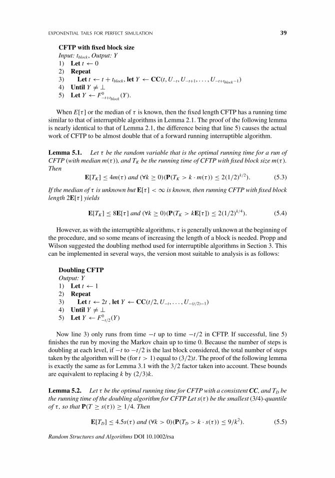
As before, the tripling algorithm with recursive structure can be used to give a tail thatis exponential in a polynomial in k. For CFTP, it is helpful given the current time t, to knowthe next block size s. From the recursive description, it is possible to build a method forfinding the next block size.

When t is written in base 3, the next block size will be 1 if the least significant nonzerodigit is 1, and if this digit is 2, the next block size has this digit 1 and all digits of lesssignificance 0. (See Fig. 4).

The following code calculates this value.

Block_SizeInput: t Output: s1) Let b ← 1/32) Repeat3) Let b ← 3b4) Let a be t/b modulo 35) Until a �= 06) Let s ← 1(a = 1) + (3b)1(a = 2)

Now CFTP is run as before, only the next block size comes from Block_Size rather thansimple doubling.

Tripling CFTPOutput: Y1) Let t ← 02) Repeat3) Let s ← Block_Size(t)4) Let t ← t + s4) Let Y ← CC(s, U−t , . . . , U−t+s−1)

5) Until Y �= ⊥6) Let Y ← F0

−t+s−1(Y)

The length of the final block that does not return ⊥ might be arbitrarily small comparedto the the t + s steps taken in line 6). Hence the total running time could be close to 2 timesthe final value of t. This modifies the analysis in Lemma 4.1 to give the following.

Lemma 5.3. Let τ be the optimal running time for CFTP with a consistent CC, and T3

be the running time of the tripling algorithm for CFTP. Let m(τ ) be the smallest median ofτ , and β = ln 2/ ln 3 ≈ 0.6309. Then

E[T3] ≤ 31.8m(τ ) and (∀k ≥ 0)(P(T3 > k · m(τ )) ≤ 4 exp(−0.289kβ). (5.7)




E[T3] ≤ 14E[τ ] and (∀k ≥ 0)(P(T3 > kE[τ ]) ≤ 4 exp(−0.186kβ). (5.8)

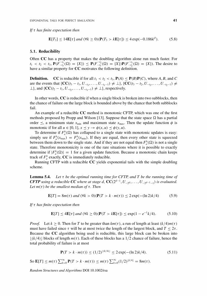
5.1. Reducibility

Often CC has a property that makes the doubling algorithm alone run much faster. Fort1 < t2 < t3, P(F−t1−t3

(�) = {X}) ≤ P(F−t2−t3(�) = {X})P(F−t1−t2

(�) = {X}). The desire tohave a similar property for CC motivates the following definition.

Definition. CC is reducible if for all t1 < t2 < t3, P(A) ≤ P(B)P(C), where A, B, and Care the events that {CC(t3 − t1, U−t3 , . . . , U−t1−1) �= ⊥}, {CC(t3 − t2, U−t3 , . . . , U−t2−1) �=⊥}, and {CC(t2 − t1, U−t2 , . . . , U−t1−1) �= ⊥}, respectively.

In other words, CC is reducible if when a single block is broken into two subblocks, thenthe chance of failure on the large block is bounded above by the chance that both subblocksfail.

An example of a reducible CC method is monotonic CFTP, which was one of the firstmethods proposed by Propp and Wilson [13]. Suppose that the state space � has a partialorder �, a minimum state xmin and maximum state xmax. Then the update function φ ismonotonic if for all u ∈ [0, 1], x � y → φ(x, u) � φ(y, u).

To determine if Fba (�) has collapsed to a single state with monotonic updates is easy:

simply see if Fba (xmax) = Fb

a (xmin). If they are equal, then every other state is squeezedbetween them down to the single state. And if they are not equal then Fb

a (�) is not a singlestate. Therefore monotonicity is one of the rare situations where it is possible to exactlydetermine if |Fb

a (�)| = 1 for a given update function. Because a monotonic chain keepstrack of Fb

a exactly, CC is immediately reducible.Running CFTP with a reducible CC yields exponential tails with the simple doubling

scheme.

Lemma 5.4. Let τ be the optimal running time for CFTP, and T be the running time ofCFTP using a reducible CC where at stage d, CC(2d−1, U−2d , . . . , U−2d−1−1) is evaluated.Let m(τ ) be the smallest median of τ . Then

E[T ] = 8m(τ ) and (∀k > 0)(P(T > k · m(τ )) ≤ 2 exp(−(ln 2)k/4) (5.9)


E[T ] ≤ 4E[τ ] and (∀k ≥ 0)(P(T > kE[τ ]) ≤ exp(1 − e−1k/4). (5.10)

Proof. Let k ≥ 0. Then for T to be greater than km(τ ), a run of length at least (k/4)m(τ )

must have failed since τ will be at most twice the length of the largest block, and T ≤ 2τ .Because the CC algorithm being used is reducible, this large block can be broken into(k/4) blocks of length m(τ ). Each of these blocks has a 1/2 chance of failure, hence thetotal probability of failure is at most

P(T > k · m(τ )) ≤ (1/2)(k/4) ≤ 2 exp(−(ln 2)k/4). (5.11)

So E[T ] ≤ m(τ )∑∞

k=0 P(T > k · m(τ )) ≤ m(τ )∑∞

k=0(1/2)k/4 = 8m(τ ).


42 HUBER

When τ has finite expectation, then the longest block is at most 2τ , and T is twice thesize of the longest block, so E[T ] ≤ 4E[τ ]. Markov’s inequality means that the probabilitythat a block of length αE[τ ] fails is at most 1/α. Putting that into the argument for m(τ )

yieldsP(T > k · E[τ ]) ≤ α exp(−(ln α)α−1k/4). (5.12)

Setting α = e maximizes (ln α)/α, and yields the rest of (5.10).

There are ways other than monotonicity for creating a reducible CC. For example, themethod of bounding chains (see [8] for details) will generate CC algorithms with thisproperty as well.

6. INTERRUPTIBILITY

The reason why the exponential tails are so important for CFTP is because CFTP is not aninterruptible algorithm. This introduces an unknown amount of bias to the samples basedon the (typically unknown or unacknowledged) user impatience. The exponential tail ishelpful in that the user impatience is unlikely to have a large impact as long as the usercommits to running at least a constant times the expected running time.

Dyer and Greenhill [3] noted that any rapidly mixing Markov chain can be turned into anoninterruptible exact sampling algorithm. Without going into details, the running time oftheir method is polynomial p(n) with extremely high probability, and exponential x(n) withextremely small probability. (Here n measures the size of the problem input.) As long asthe x(n) branch is taken with small enough probability, the overall expected running timewill be polynomial.

Of course, in practice if the x(n) branch is taken, the user would actually abort theprocedure. This is an example of an algorithm design where user interruption is expectedto happen. This is in sharp contrast to CFTP, where user interruption is typically neverexpected to happen by the user. This is usually an unjustified assumption on the part of theuser since in reality a CFTP algorithm could be interrupted at any time.

However, the exponential declining tail on the running time for CFTP explains why withpractitioners this has never been an issue: with the doubling algorithm and a reducible CCalgorithm a user could run millions of iterations and still be extremely unlikely to have todouble more than a few times more than average.

ACKNOWLEDGEMENTS

The author thanks Wilfrid Kendall for several helpful discussions, and the anonymousreferees for some helpful comments.

REFERENCES

[1] P. Diaconis and B. Efron, Testing for independence in a two-way table: New interpretations ofthe chi-square statistic, Ann Statist 13 (1985), 845–913.

[2] P. Diaconis and D. Stroock, Geometric bounds for eigenvalues of Markov chains, Ann ApplProbab 1 (1991), 36–61.



[3] M. Dyer and C. Greenhill, “Random walks on combinatorial objects,” Surveys in combinatorics,J. D. Lamb and D. A. Preece (Editors), London Math Soc Lecture Note Ser 267, CambridgeUniversity Press, Cambridge, 1999.

[4] J. A. Fill and M. L. Huber, The randomness recyler: A new approach to perfect sampling, Procof 41st Symp Foundations of Computer Science, 2000, pp. 503–511.

[5] J. A. Fill, M. Machida, D. J. Murdoch, and J. S. Rosenthal, Extension of Fill’s perfect rejectionsampling algorithm to general chain, Random Structures Algorithms 17 (2000), 290–316.

[6] G. S. Fishman, Choosing sample path length and number of sample paths when starting in thesteady state, Oper Res Lett 16 (1994), 209–219.

[7] O. Häggström and K. Nelander, On exact simulation from Markov random fields using couplingfrom the past, Scand J Statist 26 (1999), 395–411.

[8] M. Huber, Perfect sampling using bounding chains, Ann Appl Probab 14 (2004), 734–753.

[9] M. L. Huber, Exact sampling and approximate counting techniques, Proc 30th Symp Theoryof Computing, 2000, pp. 31–40.

[10] M. Jerrum and A. Sinclair, Approximating the permanent, J Comput 18 (1989), 1149–1178.

[11] M. Jerrum and A. Sinclair, The Markov chain Monte Carlo method: An approach to approximatecounting and integration, PWS, Boston, 1996.

[12] M. Newman and G. Barkema, Monte Carlo methods in statistical physics, Oxford UniversityPress, New York, 1999.

[13] J. G. Propp and D. B. Wilson, Exact sampling with coupled Markov chains and applicationsto statistical mechanics, Random Structures Algorithms 9 (1996), 223–252.

[14] J. G. Propp and D. B. Wilson, How to get a perfectly random sample from a generic Markovchain and generate a random spanning tree of a directed graph, J Algorithms 217 (1998),170–217.


Documents

Perfect simulation with exponential tails on the running time