Embed Size (px)
Citation preview
Short Version (8 April 2003)
PERFECT STOCHASTIC SUMMATION IN HIGH ORDER
FEYNMAN GRAPH EXPANSIONS
J.N. CORCORAN,∗ The University of Colorado
U. SCHNEIDER,∗∗ The University of Colorado
H. -B. SCHUTTLER,∗∗∗ The University of Georgia
Abstract
We describe a new application of an existing perfect sampling technique of
Corcoran and Tweedie to estimate the self energy of an interacting Fermion
model via Monte Carlo summation. Simulations suggest that the algorithm in
this context converges extremely rapidly and results compare favorably to true
values obtained by brute force computations for low dimensional toy problems.
A variant of the perfect sampling scheme which improves the accuracy of the
Monte Carlo sum for small samples is also given.
Keywords: Invariant measures; backward coupling; coupling from the past;
exact sampling; perfect sampling; IMH algorithm; Monte Carlo summation;
self energy; Feynman diagram; resummation; Hubbard model.
AMS 2000 Subject Classification: Primary 60J10;60K30
Secondary 82B80;82D25
∗ Postal address: Department of Applied Mathematics, The University of Colorado, Box 526 Boulder
CO 80309-0526, USA; email: [email protected], [email protected]; phone: 303-492-
0685∗∗ Postal address: Department of Applied Mathematics, The University of Colorado, Box 526 Boulder
CO 80309-0526, USA; email: [email protected], [email protected]; phone: 303-
735-1024∗∗∗ Postal address: Center for Simulational Physics, Department of Physics and Astronomy, The
University of Georgia, Athens GA 30602, USA; email: [email protected]; phone: 706-542-3886
1
2 J.N. Corcoran, U. Schneider, and H. -B. Schuttler
1. Introduction
The interacting fermion problem is of fundamental importance in a wide range
of research areas, including fields as diverse as electronic structure theory of solids,
strongly correlated electron physics, quantum chemistry, and the theory of nuclear
matter [6, 11, 15]. The ultimate objective of this project, which is a massive collab-
orative effort between physicists, statisticians, and computer scientists, is to combine
Monte Carlo summation techniques with self-consistent high-order Feynman diagram
expansions into an efficient tool for the controlled approximate solution of interacting
fermion models.
The concept of “self energy” is one of the most important examples of the power
of Feynman diagram resummation. Suppose, for example that we have a lattice of
atoms (such as in the case of a crystal) where electrons are almost localized in atomic
orbitals at each site. Suppose further that we create a particle at one site and destroy a
particle at another site thereby adding and removing a quanta of vibrational energy to
the system. Electrons of opposite spin occupying a single atom give rise to a Coulomb
repulsion energy which causes particles to hop between sites. There is a contribution
to the energy of the particle due to the virtual emission and absorption of particles. In
other words, the particle interacts with its surrounding medium which, in turn, acts
back on the particle. Essentially, a “wake” of energy is created around the movement
of the particle. It is this “self energy”, described in more detail in Section 2.1, that we
would like to quantify.
Self energy is represented as a large and complicated sum (“outer sum”) of terms
that are, in themselves, large and complicated sums (“inner sums”). The objective of
this paper is to describe the evaluation of these inner sums via a Monte Carlo approach.
Monte Carlo summation techniques, detailed in Section 3, involve evaluating an ap-
proximating sum at random points drawn from a particular distribution. While there
is much flexibility in the choice of this distribution, some choices are better than others
in terms of minimizing the (first level)error in the approximating sum. The downside
to choosing a nearly optimal distribution is that we often cannot sample points from
it directly and are faced with a second level of error (sampling error) resulting from a
Monte Carlo sampling approach. In this paper we choose a nearly optimal complicated
Perfect Stochastic Summation in High Order Feynman Graph Expansions 3
distribution, yet sample from it using “perfect” simulation techniques, described in
Section 4, that completely eliminate the second level error.
2. Self Energy, Feynman Diagrams, and Computer Friendly
Representation
The Hubbard model was originally developed in the early sixties in order to under-
stand the magnetic properties of electron motion in transition metals. The original
model remains a subject of active research today, and it is within this context that we
describe our numerical approach. (The approach applies, with minor adaptations, to
all interacting fermion models which possess a Feynman diagram expansion in terms
of a two-body interaction potential.)
Suppose we have a lattice of atoms, representing atoms in a crystal, where electrons
are almost localized in atomic orbitals at each site. We consider the following model
Hamiltonian governing the motion and interactions between the particles.
H =∑
j′ ,j
1
2Vj′ ,j nj′ nj −
∑
j′,j
∑
σ
tj′,j c†j′σcj σ (1)
Here
c†j′σ = creation operator that creates an electron of spin σ =↑, ↓ at site j ′
cj σ = destruction operator that destroys an electron of spin σ =↑, ↓ at site j
c†j′σ cj σ = transfers an electron of spin σ from site j to site j ′
nj = the number of electrons at site j.
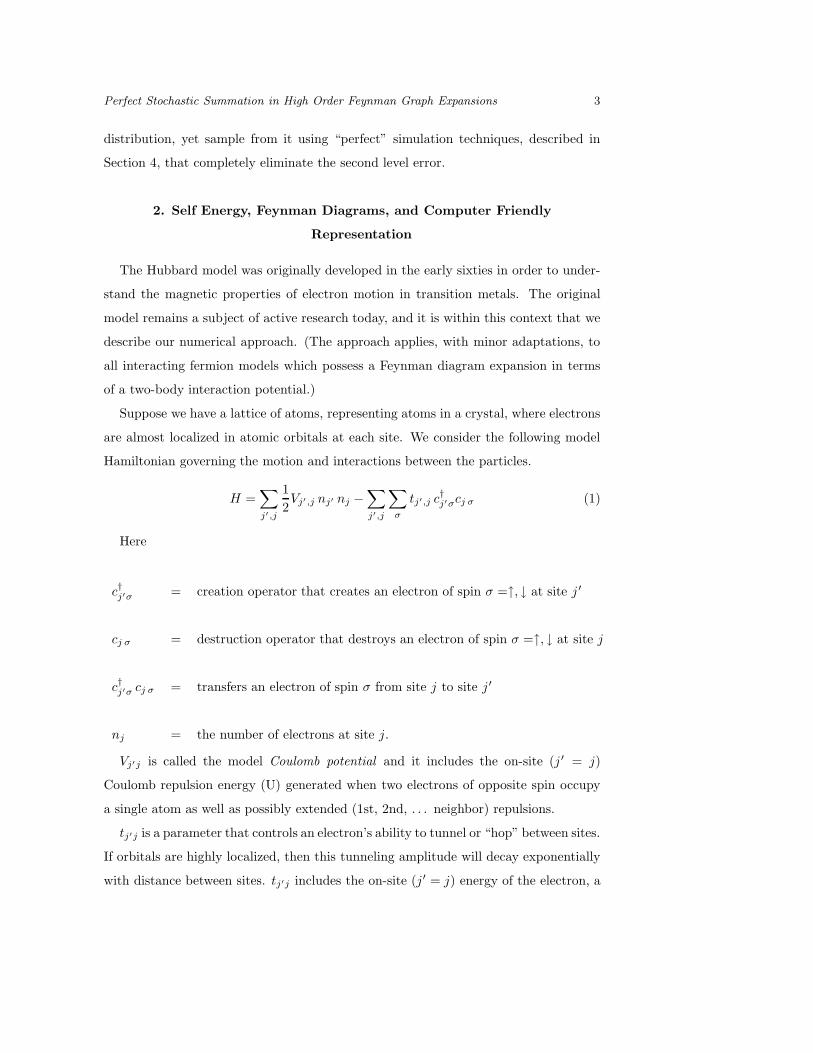
Vj′j is called the model Coulomb potential and it includes the on-site (j ′ = j)
Coulomb repulsion energy (U) generated when two electrons of opposite spin occupy
a single atom as well as possibly extended (1st, 2nd, . . . neighbor) repulsions.
tj′j is a parameter that controls an electron’s ability to tunnel or “hop” between sites.
If orbitals are highly localized, then this tunneling amplitude will decay exponentially
with distance between sites. tj′j includes the on-site (j′ = j) energy of the electron, a

4 J.N. Corcoran, U. Schneider, and H. -B. Schuttler
nearest neighbor tunneling amplitude (t) and possibly extended (2nd, 3rd . . . neighbor)
tunneling amplitudes.
The total energy, given by (1), of this Hubbard model is thus represented as a sum
of potential and kinetic energy given by the first and second terms, respectively, of (1).
Both Vj′j and tj′j are assumed to obey period boundary conditions on a finite lattice
defined in Section 2.1.
2.1. Self Energy and Feynman Diagrams
The concept of self energy enables us to understand the feedback of the interacting
environment on a propagating particle. Physically, it describes the cloud of particle-
hole excitations that form the wake which accompanies a propagating electron.
The following paragraphs describe how to obtain the self energy Σ(k). Basically, we
will depict Σ(k) through Feynman graph expansions and represent it as is a sum (of
sums) involving Green’s functions. (These Green’s functions will in turn involve the
self energy Σ(k) we are trying to compute. This issue is addressed in Section 5.)
Green’s function G(k)
The single-fermion Green’s function G(k) is the most basic physical quantity which
can be obtained via a Feynman graph expansion. As it is expressed in terms of self
energy, which we will denote by Σ(k), we will describe our approach within this context.
Here k ≡ (~k, iν) denotes a D+1-dimensional “momentum-energy” variable (referred to
as “momentum” hereafter), where ~k is a D-dimensional “wavevector” and iν represents
a frequency. These variables will be described in more detail later in this Section.
In general, a Green’s function is the response of a linear system to a point input. Di-
agrammatically, we can represent the single-fermion Green’s function, or propagator, as
a sum of free propagators with various inserted scattering processes. (Mathematically,
a propagator is simply an integral kernel.) The self energy represents all scattering
processes combined into a single quantity. We depict the Green’s function in terms of
the self energy in Figure 1.
The self energy is in turn represented as a sum of Feynman diagrams as shown in
Figure 2. These diagrams, developed by physicist Richard Feynman, give a conve-
nient shorthand for representing complex mathematical quantities. The “wavy” lines
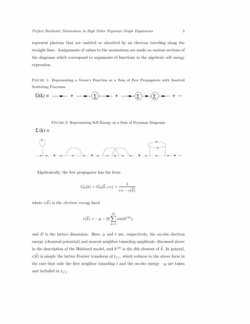
Perfect Stochastic Summation in High Order Feynman Graph Expansions 5
represent photons that are emitted or absorbed by an electron traveling along the
straight lines. Assignments of values to the momentum are made on various sections of
the diagrams which correspond to arguments of functions in the algebraic self energy
expression.
Figure 1: Representing a Green’s Function as a Sum of Free Propagators with Inserted
Scattering Processes
= + Σ + Σ Σ + ...G(k)
Figure 2: Representing Self Energy as a Sum of Feynman Diagrams
(k) = Σ
...++++
Algebraically, the free propagator has the form
G0(k) = G0(~k, i ν) =1
i ν − ε(~k)
where ε(~k) is the electron energy band
ε(~k) = −µ − 2t
D∑
d=1
cos(k(d)),
and D is the lattice dimension. Here, µ and t are, respectively, the on-site electron
energy (chemical potential) and nearest neighbor tunneling amplitude, discussed above
in the description of the Hubbard model, and k(d) is the dth element of ~k. In general,
ε(~k) is simply the lattice Fourier transform of tj′j , which reduces to the above form in
the case that only the first neighbor tunneling t and the on-site energy −µ are taken
and included in tj′j .
6 J.N. Corcoran, U. Schneider, and H. -B. Schuttler
Following the Green’s function representation from Figure 1, we may write
G(k) = G0 + G0ΣG0 + G0ΣG0ΣG0 + · · ·
= G0 + G0ΣG0 + G0(ΣG0)2 + · · ·
= 1G−1
0−Σ
by summing the Taylor series expansion in powers of (ΣG0).
This is known as the Dyson equation [11, 15]:
G(k) = G(~k, i ν) = [i ν − ε(~k) − Σ(k)]−1. (2)
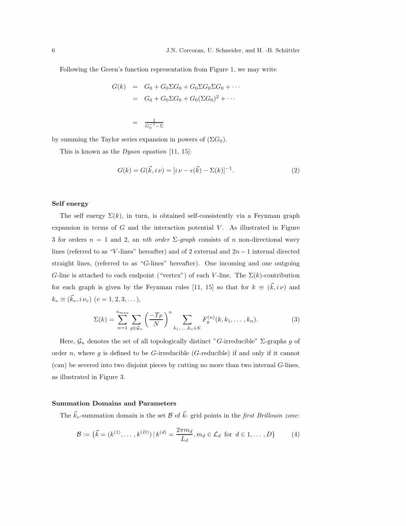
Self energy
The self energy Σ(k), in turn, is obtained self-consistently via a Feynman graph
expansion in terms of G and the interaction potential V . As illustrated in Figure
3 for orders n = 1 and 2, an nth order Σ-graph consists of n non-directional wavy
lines (referred to as “V -lines” hereafter) and of 2 external and 2n− 1 internal directed
straight lines, (referred to as “G-lines” hereafter). One incoming and one outgoing
G-line is attached to each endpoint (“vertex”) of each V -line. The Σ(k)-contribution
for each graph is given by the Feynman rules [11, 15] so that for k ≡ (~k, i ν) and
kv ≡ (~kv , i νv) (v = 1, 2, 3, . . . ),
Σ(k) =
nmax∑
n=1
∑
g∈Gn
(
−TP
N
)n∑
k1,... ,kn∈K
F (n)g (k, k1, . . . , kn). (3)
Here, Gn denotes the set of all topologically distinct ”G-irreducible” Σ-graphs g of
order n, where g is defined to be G-irreducible (G-reducible) if and only if it cannot
(can) be severed into two disjoint pieces by cutting no more than two internal G-lines,
as illustrated in Figure 3.
Summation Domains and Parameters
The ~kv-summation domain is the set B of ~k- grid points in the first Brillouin zone:
B := {~k = (k(1), . . . , k(D)) | k(d) =2πmd
Ld, md ∈ Ld for d ∈ 1, . . . , D} (4)
Perfect Stochastic Summation in High Order Feynman Graph Expansions 7
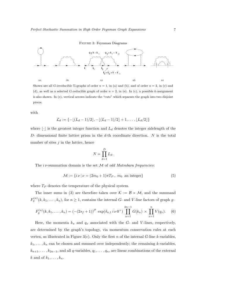
Figure 3: Feynman Diagrams
k2
2 1 2
1
3 1k = k + k − k2
k
(c)(b)(a) (d) (e)
k
q = k − k1q = k − k1
Shown are all G-irreducible Σ-graphs of order n = 1, in (a) and (b), and of order n = 2, in (c) and
(d), as well as a selected G-reducible graph of order n = 2, in (e). In (c), a possible k-assignment
is also shown. In (e), vertical arrows indicate the “cuts” which separate the graph into two disjoint
pieces.
with
Ld := {−b(Ld − 1)/2c,−b(Ld − 1)/2c+ 1, . . . , bLd/2c}
where b·c is the greatest integer function and Ld denotes the integer sidelength of the
D- dimensional finite lattice prism in the d-th coordinate direction. N is the total
number of sites j in the lattice, hence
N =
D∏
d=1
Ld.
The i ν-summation domain is the set M of odd Matsubara frequencies :
M := {i ν | ν = (2m0 + 1)πTP , m0 an integer} (5)
where TP denotes the temperature of the physical system.
The inner sums in (3) are therefore taken over K := B × M, and the summand
F(n)g (k, k1, . . . , kn), for n ≥ 1, contains the internal G- and V -line factors of graph g:
F (n)g (k, k1, . . . , kn) = (−(2sf + 1))lg exp(δn,1 i ν 0+)
2n−1∏
u=1
G(ku) ×
n∏
x=1
V (qx). (6)
Here, the momenta ku and qx associated with the G- and V -lines, respectively,
are determined by the graph’s topology, via momentum conservation rules at each
vertex, as illustrated in Figure 3(c). Only the first n of the internal G-line k-variables,
k1, . . . , kn can be chosen and summed over independently; the remaining k-variables,
kn+1, . . . , k2n−1, and all q-variables, q1, . . . , qn, are linear combinations of the external
k and of k1, . . . , kn.
8 J.N. Corcoran, U. Schneider, and H. -B. Schuttler
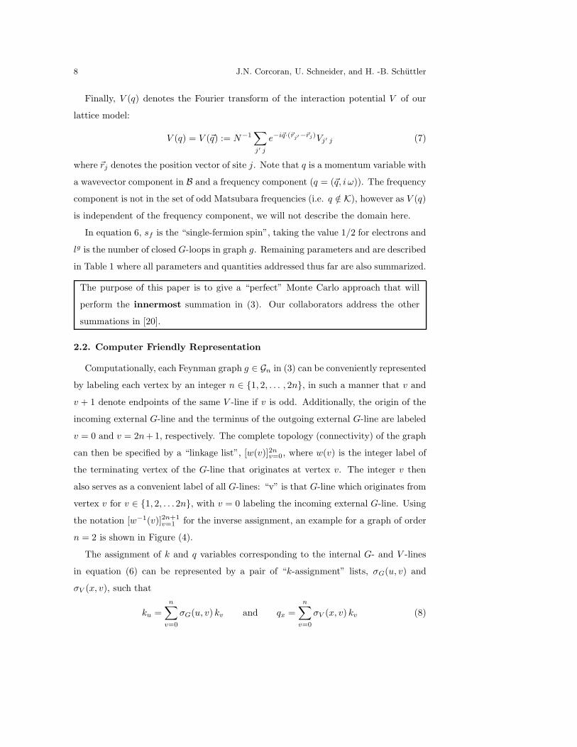
Finally, V (q) denotes the Fourier transform of the interaction potential V of our
lattice model:
V (q) = V (~q) := N−1∑
j′ j
e−i~q·(~rj′−~rj)Vj′ j (7)
where ~rj denotes the position vector of site j. Note that q is a momentum variable with
a wavevector component in B and a frequency component (q = (~q, i ω)). The frequency
component is not in the set of odd Matsubara frequencies (i.e. q /∈ K), however as V (q)
is independent of the frequency component, we will not describe the domain here.
In equation 6, sf is the “single-fermion spin”, taking the value 1/2 for electrons and
lg is the number of closed G-loops in graph g. Remaining parameters and are described
in Table 1 where all parameters and quantities addressed thus far are also summarized.
The purpose of this paper is to give a “perfect” Monte Carlo approach that will
perform the innermost summation in (3). Our collaborators address the other
summations in [20].
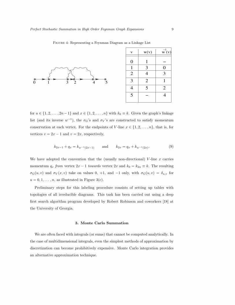
2.2. Computer Friendly Representation
Computationally, each Feynman graph g ∈ Gn in (3) can be conveniently represented
by labeling each vertex by an integer n ∈ {1, 2, . . . , 2n}, in such a manner that v and
v + 1 denote endpoints of the same V -line if v is odd. Additionally, the origin of the
incoming external G-line and the terminus of the outgoing external G-line are labeled
v = 0 and v = 2n+ 1, respectively. The complete topology (connectivity) of the graph
can then be specified by a “linkage list”, [w(v)]2nv=0, where w(v) is the integer label of
the terminating vertex of the G-line that originates at vertex v. The integer v then
also serves as a convenient label of all G-lines: “v” is that G-line which originates from
vertex v for v ∈ {1, 2, . . .2n}, with v = 0 labeling the incoming external G-line. Using
the notation [w−1(v)]2n+1v=1 for the inverse assignment, an example for a graph of order
n = 2 is shown in Figure (4).
The assignment of k and q variables corresponding to the internal G- and V -lines
in equation (6) can be represented by a pair of “k-assignment” lists, σG(u, v) and
σV (x, v), such that
ku =n∑
v=0
σG(u, v) kv and qx =n∑
v=0
σV (x, v) kv (8)
Perfect Stochastic Summation in High Order Feynman Graph Expansions 9
Figure 4: Representing a Feynman Diagram as a Linkage List
−1v w(v) w (v)
3 2 1
4 5 2
5 − 4
0 51 23 4
0 1 −
2 4 31 3 0
for u ∈ {1, 2, . . . , 2n− 1} and x ∈ {1, 2, . . . , n} with k0 ≡ k. Given the graph’s linkage
list (and its inverse w−1), the σG’s and σV ’s are constructed to satisfy momentum
conservation at each vertex. For the endpoints of V -line x ∈ {1, 2, . . . , n}, that is, for
vertices v = 2x − 1 and v = 2x, respectively,
k2x−1 + qx = kw−1(2x−1) and k2x = qx + kw−1(2x). (9)
We have adopted the convention that the (usually non-directional) V -line x carries
momentum qx from vertex 2x − 1 towards vertex 2x and k0 = k2n ≡ k. The resulting
σG(u, v) and σV (x, v) take on values 0, +1, and −1 only, with σG(u, v) = δu,v for
u = 0, 1, . . . , n, as illustrated in Figure 3(c).
Preliminary steps for this labeling procedure consists of setting up tables with
topologies of all irreducible diagrams. This task has been carried out using a deep
first search algorithm program developed by Robert Robinson and coworkers [18] at
the University of Georgia.
3. Monte Carlo Summation
We are often faced with integrals (or sums) that cannot be computed analytically. In
the case of multidimensional integrals, even the simplest methods of approximation by
discretization can become prohibitively expensive. Monte Carlo integration provides
an alternative approximation technique.
10 J.N. Corcoran, U. Schneider, and H. -B. Schuttler
Suppose we wish to evaluate the integral
I(g, A) =
∫
A
g(x)dx (10)
for some integrable function g : IRn → IR and some set A ⊆ IRn. Let π(x) be any
probability density function whose support contains A. Then we may write
I(g, A) =
∫
A
g(x)dx =
∫
IRn
g(x)1lA(x)dx =
∫
IRn
g(x)1lA(x)
π(x)π(x)dx
where 1lA(x) is the indicator function. We shall refer to π(x) as the weight function
and the remaining part of the integrand as the score function.
Now if X is a random variable with density π(x), we find that we have written the
integral as an expected value
I(g, A) = E
[
g(X)1lA(X)
π(X)
]
. (11)
A basic Monte Carlo integration technique is to simulate independent and identically
distributed (i.i.d.) values drawn from the distribution with density π(x), say
X1, X2, . . . , Xniid∼ π
and to estimate the probability weighted average given in (11) by
I(g, A) =1
n
n∑
i=1
g(Xi)1lA(Xi)
π(Xi). (12)
Clearly, by (11), this is an unbiased estimator of I(g, A).
Since the variance of this estimator is
V [I(g, A)] = 1n V
[
g(X)1lA(X)π(X)
]
= 1n E
[
(
g(X)1lA(X)π(X) − I(g, A)
)2]
,
the variance is minimized by choosing
π(x) =|g(x)|1lA(x)
∫
IRn |g(x)|1lA(x) dx. (13)
Specifically, we choose
π(x) =
|g(x)|R
A|g(x)|dx
, x ∈ A
0 , x /∈ A
(14)
Perfect Stochastic Summation in High Order Feynman Graph Expansions 11
Of course, if we could compute the denominator for this optimal “weight”, it is likely
that we could have solved our original problem and there is no need to use a Monte
Carlo approach to compute the integral in (10). Hence, we may consider taking a
different, non-optimal candidate weight, keeping in mind that we would like to at least
choose something that attempts to mimic the shape of g. We point out that while we
may usually sample from (14) without knowing the constant of proportionality, (for
example using the Metropolis-Hastings algorithm), we ultimately require the constant
in order to evaluate (12).
4. Perfect Simulation
There has been considerable recent work on the development and application of
“perfect sampling” algorithms that will enable the simulation of the invariant (or
stationary) measure π of a Markov chain, either exactly (that is, by drawing a random
sample known to be from π) or approximately, but with computable order of accuracy.
These were sparked by the seminal paper of Propp and Wilson [17], and several
variations and extensions of this idea have appeared since – see [3, 4, 5, 7, 8, 12], and
[14]. These ideas have proven effective in areas such as statistical physics, spatial point
processes and operations research, where they provide simple and powerful alternatives
to methods based on iterating transition laws, for example.
The essential idea of most of these approaches is to find a random epoch −T (not
to be confused with the physical temperature of the system being considered in this
paper) in the past such that, if we construct sample paths (according to a transition
law P (x, y) that is invariant for π) from every point in the state space starting at
−T , then all paths will have coupled successfully by time zero. The common value of
the paths at time zero is a draw from π. Intuitively, it is clear why this result holds
with such a random time T . For consider a chain starting at −∞ with the stationary
distribution π. At every iteration it maintains the distribution π. But at time −T it
must pick some value x, and from then on it follows the trajectory from that value.
But of course it arrives at the same place at time zero no matter what value x is picked
at time −T : so the value returned by the algorithm at time zero must itself be a draw
from π.
12 J.N. Corcoran, U. Schneider, and H. -B. Schuttler
Perfect sampling algorithms can be particularly efficient if the chain is stochastically
monotone in the sense that paths from lower starting points stay below paths from
higher starting points. In this case, one need only couple sample paths from the
“top” and “bottom” of the space, as all other paths will be sandwiched in between.
It is possible to generalize one step further to monotone chains on an unbounded
state space by considering stochastically dominating processes to bound the journeys
of sample paths. For example, see [8].
For this to be practicable we need to ensure that T is indeed finite. In [17] it is
shown that this occurs for irreducible aperiodic finite space chains, and for a number
of stochastically monotone chains possessing maximal and minimal elements. Indeed,
in [2] it is shown that if the distribution at −∞ is any fixed (or even random) value
x0, then under fairly standard conditions the value at time zero is still distributed
according to π, and this observation is crucial for perfect sampling algorithms.
There are several easy-to-read perfect sampling tutorials available, and we refer
interested readers to [1]. In this paper we only wish to emphasize that the key idea
in the search successively further and further back in time for the so-called backward
coupling time T requires that one reuse random number streams. That is, if sample
paths run forward to time 0 from time −1 using a random number (or random vector)
U−1 have not coalesced by time 0, then one must go back further, say to time −2 and
run paths forward for two steps using a random number U−2 and then the previously
used U−1.
We now describe a particular specific perfect sampling scheme that we will use for
our self energy calculations.
4.1. The IMH Algorithm
Certain monotonicity properties of the “independent” Metropolis-Hastings (IMH)
scheme, which we review briefly in this section, are such that perfect sampling is
feasible [2]. We use the term “independent” to describe the Metropolis-Hastings
algorithm where candidate states are generated by a distribution that is independent
of the current state of the chain. In other words, suppose we have a given candidate
distribution Q which we will assume to have a density q, positive everywhere for
convenience, with which we can generate potential values of an i.i.d. sequence. A
Perfect Stochastic Summation in High Order Feynman Graph Expansions 13
“candidate value” generated according to q is then accepted with probability α(x, y)
given by
α(x, y) =
min{
π(y)π(x)
q(x)q(y) , 1
}
π(x)q(y) > 0
1 π(x)q(y) = 0
where x is the current state and y is the candidate state.
Thus, actual transitions of the IMH chain take place according to a law P with
transition density
p(x, y) = q(y)α(x, y), y 6= x
and with probability of remaining at the same point given by
P (x, {x}) =
∫
q(y)[1 − α(x, y)]µ(dy)
where µ is Lebesgue measure. With this choice of α we have that π is invariant for P .
The perfect IMH algorithm uses the ratios in the acceptance probabilities α(x, y) to
reorder the states in such a way that we always accept moves to the left (or downwards).
That is, if we write π(x) = c h(x) where k is unknown, we define the IMH ordering,
x � y ⇔π(y)q(x)
π(x)q(y)≥ 1 ⇔
h(y)
q(y)≥
h(x)
q(x)(15)
With this ordering, we can (hopefully) attain a “lowest state” l. Essentially, one
can think of l as the state that is hardest to move away from when running the IMH
algorithm. Thus, if we are able to accept a move from l to a candidate state y drawn
from the distribution Q with density q, then sample paths from every point in the
state space will also accept a move to y, so all possible sample paths will coalesce. The
perfect sampling algorithm is formally described as follows:
IMH (Backward Coupling) Algorithm
1. Draw a sequence of random variables Qn ∼ Q for n = 0,−1,−2, . . . , and a
sequence αn ∼ unif(0, 1) for n = −1,−2, . . . .
2. For each time −n = −1,−2, . . . , start a lower path L at l, and an upper path, U
at Q−n.
14 J.N. Corcoran, U. Schneider, and H. -B. Schuttler
3. (a) For the lower path: Accept a move from l to Q−n+1 at time −n + 1 with
probability α(l, Q−n+1), otherwise remain at state l. That is, accept the
move from l to Q−n+1 if α−n ≤ α(l, Q−n+1).
(b) For the upper path: Similarly, accept a move from Q−n to Q−n+1 at time
−n + 1 if α−n ≤ α(Q−n, Q−n+1); otherwise remain at state Q−n.
4. Continue until T defined as the first n such that at time −n + 1 each of these
two paths accepts Q−n+1. (Continue the Metropolis-Hastings algorithm foward
to time zero using the α’s and Q’s from steps 1-3 to get the draw from π at time
zero.)
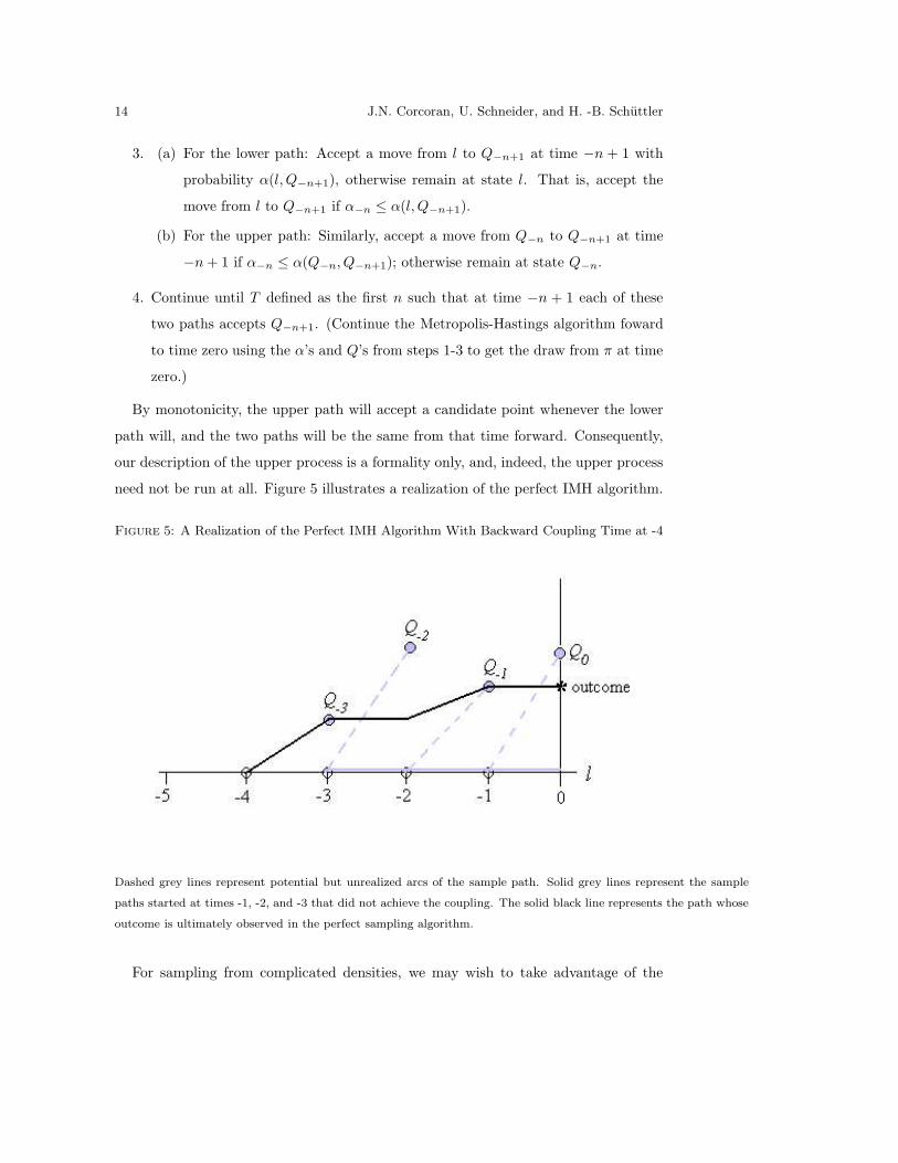
By monotonicity, the upper path will accept a candidate point whenever the lower
path will, and the two paths will be the same from that time forward. Consequently,
our description of the upper process is a formality only, and, indeed, the upper process
need not be run at all. Figure 5 illustrates a realization of the perfect IMH algorithm.
Figure 5: A Realization of the Perfect IMH Algorithm With Backward Coupling Time at -4
Dashed grey lines represent potential but unrealized arcs of the sample path. Solid grey lines represent the sample
paths started at times -1, -2, and -3 that did not achieve the coupling. The solid black line represents the path whose
outcome is ultimately observed in the perfect sampling algorithm.
For sampling from complicated densities, we may wish to take advantage of the
Perfect Stochastic Summation in High Order Feynman Graph Expansions 15
observation that neither the lowest state, l, nor the maximum value π(l)/q(l) need be
attained explicitly. If we are able to find a constant C such that
C ≥π(x)
q(x), for all x
then we know that
α(l, y) ≥π(y)
C q(y)
so we could modify step 3(a) of the IMH algorithm to read
3. (a)′ For the lower path: Accept a move from l to Q−n+1 at time −n + 1 with
probability α(l, Q−n+1), otherwise remain at state l. That is, accept the move
from l to Q−n+1 if α−n ≤ π(y)C q(y) .
We refer the reader to [2] for details on how one’s choice of Q will affect the expected
backward coupling time for the perfect IMH algorithm.
5. Perfect IMH in the Context of this Self Energy Problem
Earlier work on the Monte Carlo evaluation of individual Feynman diagrams has
employed a variety of non-perfect sampling techniques [9, 10, 19]. We now describe the
perfect IMH algorithm for computing the innermost sum in (3) for the second order
diagram depicted in Figures 3(c) and 4. Ignoring the physical constants, we would like
to compute
Σ2(k) :=∑
k1,k2∈K
3∏
u=1
G(ku) ×
2∏
x=1
V (qx). (16)
Using momentum conserving assignments, described in Section 2.2 and shown in
Figure 3(c), this becomes
Σ2(k) =∑
k1,k2∈K
G(k1) · G(k2) · G(k2 + k − k1) · V (k − k1) · V (k1 − k2). (17)
Recall that each k, k1, k2 is a D + 1-dimensional with the vector of the first D
components coming from B as decribed in (4) and the third component taking values
in
M := {i ν | ν = (2m0 + 1)πTP , m0 an integer}.
16 J.N. Corcoran, U. Schneider, and H. -B. Schuttler
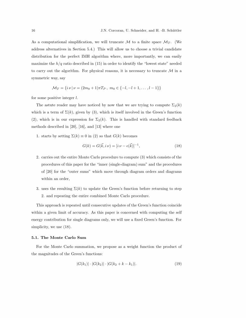
As a computational simplification, we will truncate M to a finite space MT . (We
address alternatives in Section 5.4.) This will allow us to choose a trivial candidate
distribution for the perfect IMH algorithm where, more importantly, we can easily
maximize the h/q ratio described in (15) in order to identify the “lowest state” needed
to carry out the algorithm. For physical reasons, it is necessary to truncate M in a
symmetric way, say
MT = {i ν | ν = (2m0 + 1)πTP , m0 ∈ {−l,−l + 1, . . . , l − 1}}
for some positive integer l.
The astute reader may have noticed by now that we are trying to compute Σ2(k)
which is a term of Σ(k), given by (3), which is itself involved in the Green’s function
(2), which is in our expression for Σ2(k). This is handled with standard feedback
methods described in [20], [16], and [13] where one
1. starts by setting Σ(k) ≡ 0 in (2) so that G(k) becomes
G(k) = G(~k, i ν) = [i ν − ε(~k)]−1, (18)
2. carries out the entire Monte Carlo procedure to compute (3) which consists of the
procedures of this paper for the “inner (single-diagram) sum” and the procedures
of [20] for the “outer sums” which move through diagram orders and diagrams
within an order,
3. uses the resulting Σ(k) to update the Green’s function before returning to step
2. and repeating the entire combined Monte Carlo procedure.
This approach is repeated until consecutive updates of the Green’s function coincide
within a given limit of accuracy. As this paper is concerned with computing the self
energy contribution for single diagrams only, we will use a fixed Green’s function. For
simplicity, we use (18).
5.1. The Monte Carlo Sum
For the Monte Carlo summation, we propose as a weight function the product of
the magnitudes of the Green’s functions:
|G(k1)| · |G(k2)| · |G(k2 + k − k1)|. (19)

Perfect Stochastic Summation in High Order Feynman Graph Expansions 17
However, since this involves the input external momentum k, it would be inefficient
to focus exclusively on this weight. In order to have a single weight function for any
input momentum, we again rewrite our summation goal:
Σ2(k) =∑
k1,k2,k0∈K
V (k − k1) · V (k1 − k2) · δk,k0G(k1) · G(k2) · G(k2 + k0 − k1) (20)
where δk,k0is equal to 1 when k0 = k and equal to 0 otherwise.
Now we may write
Σ2(k) =∑
k1,k2,k0∈K
S(k, k0, k1, k2) W (k0, k1, k2) (21)
where W (k0, k1, k2) is the (unnormalized) weight function
W (k0, k1, k2) = |G(k1)| · |G(k2)| · |G(k2 + k0 − k1)| (22)
and S(k, k0, k1, k2) is the score function
S(k, k0, k1, k2) = δk,k0V (k − k1) · V (k1 − k2)
G(k1) · G(k2) · G(k2 + k0 − k1)
|G(k1)| · |G(k2)| · |G(k2 + k0 − k1)|.
(23)
Our “target distribution” from which to draw values for the Monte Carlo summation
described in Section 3 is
π(k0, k1, k2) =1
NWW (k0, k1, k2) =
1
NW|G(k1)| · |G(k2)| · |G(k2 + k0 − k1)| (24)
where
NW :=∑
k0,k1,k2∈B×MT
|G(k1)| · |G(k2)| · |G(k2 + k0 − k1)|. (25)
Following Section 3 we write
Σ2(k) = NW
∑
k0,k1,k2∈B×MTS(k, k0, k1, k2) π(k0, k1, k2)
= NW E [S(K0, K1, K2)]
where (K0, K1, K2) is a random vector with density π(k0, k1, k2).
18 J.N. Corcoran, U. Schneider, and H. -B. Schuttler
5.2. The IMH Algorithm
We will now describe how to use the perfect IMH algorithm to draw n values,
(k0i, k1i, k2i), from π(k0, k1, k2). We will use these values both to estimate NW and to
plug them into the Monte Carlo approximation
Σ2(k) := NW1
n
n∑
i=1
S(k, k0i, k1i, k2i). (26)
(Note: Due to the large number of symbols in use, we are reclaiming the use of the
letter n throughout Section 5 where we are considering a fixed diagram of order 2. In
previous sections, n was reserved for a diagram order.)
In the notation of Section 4.1, the unnormalized target density is
h(k0, k1, k2) ≡ W (k0, k1, k2)
which is given by (22).
We choose a simple uniform candidate distribution with density q(k0, k1, k2) which
gives equal weight to all points (k0, k1, k2) ∈ (B ×MT )3.
In order to implement the IMH algorithm, it remains to identify the “lowest point”,
(k∗0 , k∗
1 , k∗2), which is the point in (B ×MT )3 that maximizes the ratio h/q. Since q is
constant for all (k0, k1, k2) ∈ (B ×MT )3, we simply want to maximize
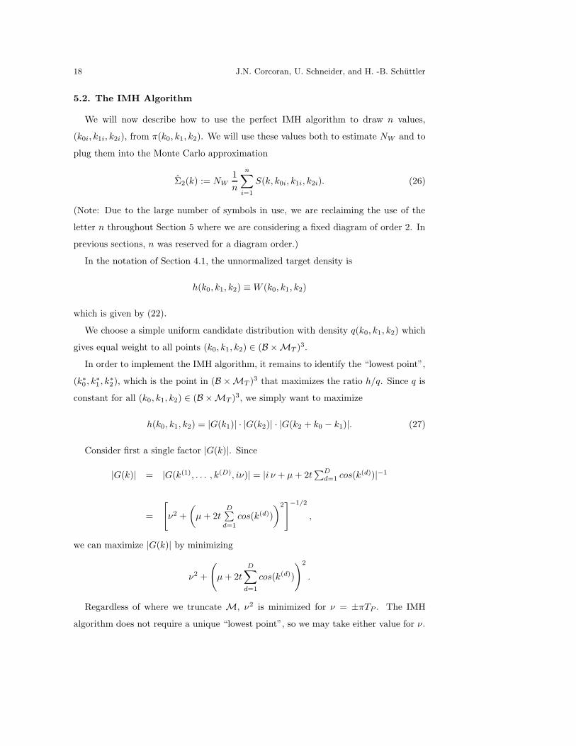
h(k0, k1, k2) = |G(k1)| · |G(k2)| · |G(k2 + k0 − k1)|. (27)
Consider first a single factor |G(k)|. Since
|G(k)| = |G(k(1), . . . , k(D), iν)| = |i ν + µ + 2t∑D
d=1 cos(k(d))|−1
=
[
ν2 +
(
µ + 2tD∑
d=1
cos(k(d))
)2]−1/2
,
we can maximize |G(k)| by minimizing
ν2 +
(
µ + 2tD∑
d=1
cos(k(d))
)2
.
Regardless of where we truncate M, ν2 is minimized for ν = ±πTP . The IMH
algorithm does not require a unique “lowest point”, so we may take either value for ν.
Perfect Stochastic Summation in High Order Feynman Graph Expansions 19
We minimize
(
µ + 2t
D∑
d=1
cos(k(d))
)2
with brute force by searching over the (finite) space B. It turns out that we only
need to do this once for the extire self energy calculation. This does not depend on
the particular graph we are considering at any moment and also therefore, just as
importantly, does not depend on the number of k’s associated with a graph.
At this point we have identified a k∗ = (~k∗, i πTP ) that maximzes |G(k)|. We may
simultaneously maximize all factors in (27) by setting each of k0, k1, and k2 to be
k∗. Due to the relationships given by (9), we will always be able to simultaneously
maximize all factors in the weight function associated with any Feynman graph in this
way.
As Σ2(k) and ultimately Σ(k) is complex-valued, the denominator of the updated,
self-consistent Green’s function obtained through the feedback procedure described
in Section 5 will have an imaginary component that is not simply in the set MT .
In this case, we will have to maximize |G(k)| by searching over values for ~k and ν
together. This does not require searching over the entire space (B ×MT ) but rather
it can be done with some finite upper-limit cut-off on |i ν| since for very large i ν,
Σ(k) is bounded by a constant independent of i ν. This fact will be especially useful
when we want to use the entire set M (described in Section 5.4) as opposed to the
truncated set MT . The foregoing procedure (of choosing W and then maximizing W
by individually maximizing each contributing |G(ki)|-factor) can be straightfowardly
generalized to higher order diagrams. The method is thus applicable at all diagram
orders with arbitrarily updated input Green’s function G(k).
5.3. Estimating NW
In order to estimate the normalization constant NW , we take advantage of com-
putations already performed within the IMH algorithm. In executing the algorithm,
we are drawing values uniformly from the space (B × MT )3. Hence, letting M :=
20 J.N. Corcoran, U. Schneider, and H. -B. Schuttler
#(
(B ×MT )3)
denote the number of points in the space, we write NW as
NW =∑
(B×MT )3 h(k0, k1, k2)
=∑
(B×MT )3h(k0,k1,k2)
1/M1M
= E
[
h(K0,K1,K2)1/M
]
= M · E[
h(K0,K1,K2)1/M
]
where (K0, K1, K2) is a random vector with uniform density on (B ×MT )3.
We estimate this expectation by drawing n points uniformly over (B ×MT )3 and
computing
NW :=M
n
n∑
i=1
h(k0i, k1i, k2i)
where (k0i, k1i, k2i) are the uniform draws.
5.4. Extending the M- Space
In order to execute the perfect IMH algorithm, we need to be able to identify the
point that maximizes h/q where h is the (possibly unnormalized) target density and q
is a candidate density with the same support as h from which we are able to simulate
values. The truncation of M is a common practice, irrespective of the algorithm to be
used, that simplifies computational cost. This turned out to be very convenient for us
as well since it provided us with a finite state space that allowed us to choose a very
simple uniform candidate density which exchanged our task of maximizing h/q for the
simpler task of maximizing only h. Another nice feature of this model is that we are
able to make MT arbitrarily large (but finite) without any adjustment, as h is always
maximized at ν = ±i πTP .
It is possible that one can use the full space M provided one chooses a candidate
density q on B ×M for which the maximizing point for h/q can be identified. If this
is not the case, one alternative is to approximate the maximum either with traditional
deterministic optimizers or a stochastic search approach. We are currently investigating
the effect of this approximation on the perfect IMH algorithm and preliminary results
suggest this “imperfect perfect simulation algorithm” is still superior to traditional
Monte Carlo methods in terms of both accuracy and speed.

Perfect Stochastic Summation in High Order Feynman Graph Expansions 21
6. Simulation Results
We ran IMH simulations for very low dimensional toy cases where our results could
be compared to those from brute force calculations and for (more interesting) higher
dimensional cases in order to verify that the algorithm is practicable in terms of speed.
In the low dimensional cases we were able to exactly reproduce the brute force results.
In the high dimensional cases, we were able to draw “perfectly” from the weight
function in a reasonable amount of time (For example we drew values with an average
backward coupling time of 12 time steps for a 9-dimensional state space that contained
8.6 × 10¹⁵ points.) but the δk,k0factor in the score function forced us to effectively
disregard more than 99% of the values when estimating Σ2(k). One possibility for fixing
this “low score problem” is to use conditional averaging in order to rewrite the score
function, removing the ”δ-spike”, while preserving the weight function. We choose to
present another possibility in Section 6.1.
6.1. Using IMH Step 3(a)′
In Section 6 we used the basic perfect IMH algorithm to draw values from the weight
function given by (22) as opposed to the somewhat more natural weight function given
by (19):
W (k, k1, k2) = |G(k1)| · |G(k2)| · |G(k2 + k − k1)|
where k is the external user-input momentum vector that is fixed for any given Σ2(k)
calculation. The purpose of using (22) was so that it would be unnecessary to change
the sampling procedure each time we wanted to change the input k. However, there
are two obvious drawbacks to this approach:
1. We increase the size of our state space. In this example, we go from having to
sample values for (k1, k2) to having to sample values for (k0, k1, k2).
2. Even with an efficient approach to sampling from the weight function, the δk,k0
in the score function causes us to effectively discard most of the sampled values.
In Section 6, the score function turned out to be zero approximately 87.5% of
the time in Example 1 and almost 100% of the time in Example 2.

22 J.N. Corcoran, U. Schneider, and H. -B. Schuttler
In this section, we consider sampling directly from (19) in order to avoid the two
drawbacks listed above. We can actually write down a single procedure that is efficient
in the sense that will work for any k if we can accept the trade-off that it may become
inefficient in some cases due to increased backward coupling times. (In some cases,
however they may decrease since we will be making the state space smaller.)
For any fixed k, we write Σ2(k) as
Σ2(k) =∑
k1,k2∈K V (k − k1) · V (k1 − k2) · G(k1) · G(k2) · G(k2 + k − k1)
=∑
k1,k2∈K V (k − k1) · V (k1 − k2)G(k1)·G(k2)·G(k2+k−k1)
|G(k1)|·|G(k2)|·|G(k2+k−k1)|
= S(k, k1, k2) Wk(k1, k2)
where S(k, k1, k2) is the score function
S(k, k1, k2) :=V (k − k1) · V (k1 − k2) · G(k1) · G(k2) · G(k2 + k − k1)
|G(k1)| · |G(k2)| · |G(k2 + k − k1)|
and Wk(k1, k2) is the weight function
Wk(k1, k2) := |G(k1)| · |G(k2)| · |G(k2 + k − k1)|.
We wish to use the perfect IMH algorithm to draw values from
π(k1, k2) ∝ h(k1, k2) ≡ Wk(k1, k2).
We again choose a simple uniform candidate distribution this time with density
q(k1, k2) which gives equal weight to all points (k1, k2) ∈ (B ×MT )2.
In order to implement the IMH algorithm, it remains to identify the “lowest point”,
(k∗1 , k∗
2), which is the point in (B × MT )2 that maximizes the ratio h/q. Since q is
constant for all (k1, k2) ∈ (B ×MT )2, we simply want to maximize
h(k1, k2) = |G(k1)| · |G(k2)| · |G(k2 + k − k1)|. (28)
As in Section 5.2 we can, after a limited search, identify a point k∗ = (~k∗, i πT )
(where ~k∗ is two dimensional) that maximizes |G(k)|. This time however, it is more
difficult to simultaneously maximize all factors in (28) as we will not necessarily be able
to simply make all three arguments equal to k∗ at the same time. It is not desirable to
search through all k1 and k2 for a fixed k in order to maximize (28) for three reasons:
Perfect Stochastic Summation in High Order Feynman Graph Expansions 23
1. The search would need to be performed again each time we change the external
k.
2. The search would need to be performed again for every graph included in the
overall summation defining Σ(k).
3. The search space will increase in size with higher order graphs and, with higher
dimensions, (i.e. large D, L1, . . . , LD), it will increase much more quickly than
for the limited search described in Section 5.2.
Given that we do not want to maximize (28), we appeal to Step 3(a)′ (Section 4.1)
of the IMH algorithm.
Recall that in the IMH algorithm we move backwards in time through time steps
−1,−2,−3, . . . . At each time step, we start a sample path at the “low point”, l, and,
looking forward in time, decide whether or not the sample path is able to accept a
move to the next candidate point drawn from the candidate density q. If it will not
accept the move, we go back one more time step and try again. If it will accept the
move, we have achieved a coupling and, after following this sample path forward to
time zero, we have a draw from π.
Suppose that we are starting a sample path at the low point l and have drawn a
candidate value x from the distribution with density q. We accept a move from l to
x with probability π(x)/π(l) = h(x)/h(l). That is, we simulate a value u from the
Uniform[0,1] distribution and accept the move if
u ≤h(x)
h(l).
Suppose now that we know a value C such that h(l) ≤ C. Since
h(x)
C≤
h(x)
h(l)
we may choose to accept the move from l to x whenever
u ≤h(x)
C
since this would imply that
u ≤h(x)
h(l).
24 J.N. Corcoran, U. Schneider, and H. -B. Schuttler
In this case, we will accept moves away from l less often which result in a higher
backward coupling time, but we may still perform the IMH algorithm despite not
being able to identify l provided we can identify a C.
In the context of this problem, we have that
maxk1,k2
|G(k1)| · |G(k2)| · |G(k2 + k − k1)| ≤ |G(k∗)| · |G(k∗)| · |G(k∗)|,
so we take C to be |G(k∗)| · |G(k∗)| · |G(k∗)|.
Simulation Results
Simulations again verified low dimensional brute force calculations and produced
rapid results for high dimensional cases. For example, when simulating 100,000 values
drawn from the weight function in the case D = 2, L1 = L2 = 64 with 50 odd
Matsubara frequencies (a state space of size (64 · 64 · 50)2 = 41, 943, 040, 000), roughly
one-third of the time we only had to go back in time 1 step to acheive the coupling. In
50% of the draws, we had to go back 3 steps or less and 75% of the time the backward
coupling time was less than or equal to 9. The average backward coupling time in
100,000 draws was 20.5. This was skewed upwards by a few backward coupling times
of just over 2,000, but 90% of the draws were made in less than 33 time steps.
Acknowledgements
References
[1] Casella G., Lavine, M., and Robert, C. (2000). Explaining the perfect sampler. Working
Paper, Duke University, Durham.
[2] Corcoran, J.N. and Tweedie, R.L. (2002). Perfect sampling From Independent Metropolis-
Hastings chains. Journal of Statistical Planning and Inference 104(2), 297–314.
[3] Fill, J.A. (1998). An Interruptible Algorithm for Perfect Sampling via Markov Chains. Annals
of Applied Probability 8, 131–162.
[4] Foss, S.G. and Tweedie, R.L. (1998). Perfect simulation and backward coupling. Stochastic
Models 14, 187–203.
[5] Foss, S.G., Tweedie, R.L., and Corcoran, J.N. (1998). Simulating the invariant measures
of Markov chains using horizontal backward coupling at regeneration times. Probability in the
Engineering and Informational Sciences 12, 303–320.
Perfect Stochastic Summation in High Order Feynman Graph Expansions 25
[6] Fulde, P. (1995). Electron Correlations in Molecules and Solids, Solid State Sci., 3rd edn.
Springer, Berlin, Heidelberg.
[7] Haggstrom, O., van Liesholt, M.N.M, and Møller, J. (1999). Characterisation results
and Markov chain Monte Carlo algorithms including exact simulation for some spatial point
processes. Bernoulli 5, 641–659.
[8] Kendall, W.S. (1998). Perfect simulation for the area-interaction point process. Probability
Towards the Year 2000, 218-234. Editors L. Accardi and C.C. Heyde. Springer, New York.
[9] Kreckel R. (1997). Parallelization of adaptive MC integrators. Computational Physics Com-
munications 106, 258.
[10] Lepage, G.P. (1978). A new algorithm for adaptive multidimensional integration. Journal of
Computational Physics 27, 192.
[11] Mahan, G.D. (1990). Many Particle Physics, 2nd edn. Plenum Press, New York.
[12] Møller, J. (1999). Perfect simulation of conditionally specified models. Journal of the Royal
Statistical Society, Series B 61(1), 251–264.
[13] Monthoux, P. and Scalapino, D.J. (1994). Self-consistent dx2
−y2 pairing in a two-imensional
Hubbard model. Physical Review Letters 72, 1874.
[14] Murdoch, D.J. and Green, P.J. (1998). Exact sampling from a continuous state space.
Scandinavian Journal of Statistics 25, 483–502.
[15] Negele, J.W. and Orland, H. (1988). Quantum Many-Particle Systems. Addison Wesley,
Redwood City, CA.
[16] Pao, C. -H. and Bickers, N.E. (1994). Renormalization group acceleration of self-consistent
field solutions: two-dimensional Hubbard model. Physical Review B. 49, 1586.
[17] Propp, J.G. and Wilson, D.B. (1996). Exact sampling with coupled Markov chains and
applications to statistical mechanics. Random Structures and Algorithms 9, 223–252.
[18] Robinson, R.W. (2002). Private communication.
[19] Veseli, S. (1998). Multidimensional integration in a heterogeneous network environment.
Computational Physics Communications 108, 258.
[20] Voight, A., Liu, C., Wang, Q., Robinson R.W., and Schuttler, H. -B. (2002). Stochastic
Feynman diagram summation for the Anderson impurity model. Submitted for publication.
Preprint at: http://www.csp.uga.edu/publications/HBS/.
26 J.N. Corcoran, U. Schneider, and H. -B. Schuttler
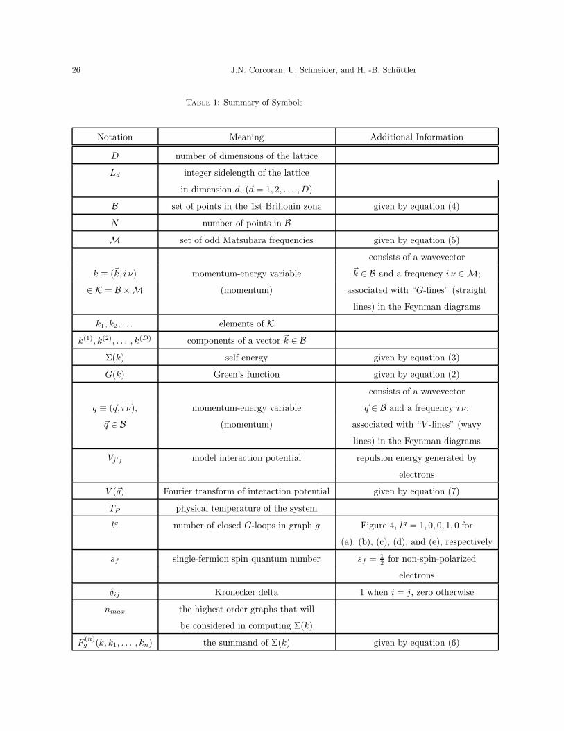
Table 1: Summary of Symbols
Notation Meaning Additional Information
D number of dimensions of the lattice
Ld integer sidelength of the lattice
in dimension d, (d = 1, 2, . . . , D)
B set of points in the 1st Brillouin zone given by equation (4)
N number of points in B
M set of odd Matsubara frequencies given by equation (5)
consists of a wavevector
k ≡ (~k, i ν) momentum-energy variable ~k ∈ B and a frequency i ν ∈ M;
∈ K = B ×M (momentum) associated with “G-lines” (straight
lines) in the Feynman diagrams
k1, k2, . . . elements of K
k(1), k(2), . . . , k(D) components of a vector ~k ∈ B
Σ(k) self energy given by equation (3)
G(k) Green’s function given by equation (2)
consists of a wavevector
q ≡ (~q, i ν), momentum-energy variable ~q ∈ B and a frequency i ν;
~q ∈ B (momentum) associated with “V -lines” (wavy
lines) in the Feynman diagrams
Vj′j model interaction potential repulsion energy generated by
electrons
V (~q) Fourier transform of interaction potential given by equation (7)
TP physical temperature of the system
lg number of closed G-loops in graph g Figure 4, lg = 1, 0, 0, 1, 0 for
(a), (b), (c), (d), and (e), respectively
sf single-fermion spin quantum number sf = 12 for non-spin-polarized
electrons
δij Kronecker delta 1 when i = j, zero otherwise
nmax the highest order graphs that will
be considered in computing Σ(k)
F(n)g (k, k1, . . . , kn) the summand of Σ(k) given by equation (6)