Embed Size (px)
Citation preview

Performance Analysis and DeploymentTechniques for Wireless Sensor Networks
Huimin She
Stockholm 2012
Thesis submitted to the KTH Royal Institute of Technology in partialfulfillment of the requirements for the degree of Doctor of Technology

She, HuiminPerformance Analysis and Deployment Techniques for Wireless SensorNet-
works
ISBN 978-91-7501-430-2TRITA-ICT/ECS AVH 12:02ISSN 1653-6363ISRN KTH/ICT/ECS/AVH-12/02-SE
Copyright © Huimin She, 2012
School of Information and Communication TechnologyKTH Royal Institute of TechnologySE-164 40 StockholmSWEDEN

Abstract
Recently, wireless sensor network (WSN) has become a promising technologywith a wide range of applications such as supply chain monitoring and environmentsurveillance. It is typically composed of multiple tiny devices equipped with lim-ited sensing, computing and wireless communication capabilities. Design of suchnetworks presents several technique challenges while dealing with various require-ments and diverse constraints. Performance analysis and deployment techniquesare required to provide insight on design parameters and system behaviors.
Based on network calculus, a deterministic analysis method is presented forevaluating the worst-case delay and buffer cost of sensor networks.To this end,traffic splitting and multiplexing models are proposed and their delay and bufferbounds are derived. These models can be used in combination to characterizecomplex traffic flowing scenarios. Furthermore, the method integrates a variableduty cycle to allow the sensor nodes to operate at low rates thus saving power.In an attempt to balance traffic load and improve resource utilization and perfor-mance, traffic splitting mechanisms are introduced for sensor networks with gen-eral topologies. To provide reliable data delivery in sensor networks, retransmis-sion has been one of the most popular schemes. We propose an analyticalmethodto evaluate the maximum data transmission delay and energy consumption of twotypes of retransmission schemes: hop-by-hop retransmission and end-to-end re-transmission. In order to validate the tightness of the bounds obtained by the anal-ysis method, the simulation results and analytical results are compared with variousinput traffic loads. The results show that the analytic bounds are correct and tight.
Stochastic network calculus has been developed as a useful tool for Qualityof Service (QoS) analysis of wireless networks. We propose a stochastic servicecurve model for the Rayleigh fading channel and then provide formulas tode-rive the probabilistic delay and backlog bounds in the cases of deterministic andstochastic arrival curves. The simulation results verify that the tightness of thebounds are good. Moreover, a detailed mechanism for bandwidth estimationofrandom wireless channels is developed. The bandwidth is derived fromthe mea-surement of statistical backlogs based on probe packet trains. It is expressed bystatistical service curves that are allowed to violate a service guarantee witha cer-tain probability. The theoretic foundation and the detailed step-by-step procedureof the estimation method are presented.
One fundamental application of WSNs is event detection in a Field of Inter-est (FoI), where a set of sensors are deployed to monitor any ongoingevents. Tosatisfy a certain level of detection quality in such applications, it is desirable thatevents in the region can be detected by a required number of sensors. Hence, an
iii

iv Abstract
important problem is how to conduct sensor deployment for achieving certain cov-erage requirements. In this thesis, a probabilistic event coverage analysis methodis proposed for evaluating the coverage performance of heterogeneous sensor net-works with randomly deployed sensors and stochastic event occurrences. More-over, we present a framework for analyzing node deployment schemesin terms ofthree performance metrics: coverage, lifetime, and cost. The method can beusedto evaluate the benefits and trade-offs of different deployment schemesand thusprovide guidelines for network designers.
Keywords: wireless sensor network, performance analysis, network calculus,coverage analysis, deployment scheme

Acknowledgments
First I would like to express sincere gratitude to my supervisor Associate Prof.Zhonghai Lu. Prof. Lu helps me a lot on my research and study, as well as onpersonal life. He is not only a good supervisor, but also a good friendto me. Manythanks to him for all the constructive comments and fruitful discussions. I willnever forget his encouragement when my papers were rejected. Special thanks goto Prof. Axel Jantsch. He has provided a very pleasant research environment forhis students. He is always supportive for my ideas and personal potentials. I wouldalso like to thank Prof. Li-Rong Zheng for introducing me to KTH. His supporthas provided a good basis for the present thesis.
I would like to thank my previous supervisors Prof. Dian Zhou and Prof. XuanZeng at Fudan university for introducing me to the world of scientific research. Iwould also thank Prof. Ahmed Hemani for reviewing my thesis. Special thanks goto Associate Prof. Ingo Sander and Dr. Qiang Chen for their help.
Many thanks are due to current and former colleagues at ES departmentandiPack center for their friendships and the pleasant atmosphere they havecreated.There are too numerous names to be mentioned here, thank you all. Also, specialthanks should go to the administrative staff at ES and the IT support groupat ICTfor their assistance in all kinds of issues.
I am grateful to all my friends in Sweden and China for the fun and encour-agement. Without you, the cold, dark winter of Stockholm could be much moreunpleasant.
I am grateful to the Vinn Excellence centers program of Vinnova (The SwedishGovernmental Agency for Innovation Systems). Without its financial support, thiswork could not have been possible.
Thanks to Prof. Yuming Jiang for being my opponent. I would also like tothank Prof. Björn Pehrson, Prof. Marko Hännikäinen, and Prof. Markus Fidler forbeing committee members.
I owe my loving thanks to my wife Liping for her understanding, continuoussupport and patience. Words are not powerful enough to express mygratefulness.In addition, I would like to thank my parents and brother for their unconditionalsupport.
Huimin She
Stockholm, Sweden, May 2012
v

vi

Contents
List of Abbreviations xv
List of Publications xvii
1 Introduction 11.1 Background . . . . . . . . . . . . . . . . . . . . . . . . . . . . . 11.2 Motivation . . . . . . . . . . . . . . . . . . . . . . . . . . . . . . 31.3 Contributions and Outline . . . . . . . . . . . . . . . . . . . . . . 6
2 Deterministic Performance Analysis 92.1 Introduction . . . . . . . . . . . . . . . . . . . . . . . . . . . . . 92.2 Related Work . . . . . . . . . . . . . . . . . . . . . . . . . . . . 102.3 Basics of Deterministic Network Calculus . . . . . . . . . . . . . 122.4 Analysis of Traffic Splitting Scheme . . . . . . . . . . . . . . . . 15
2.4.1 System Model . . . . . . . . . . . . . . . . . . . . . . . 152.4.2 Analysis . . . . . . . . . . . . . . . . . . . . . . . . . . 202.4.3 Discussions . . . . . . . . . . . . . . . . . . . . . . . . . 252.4.4 An Analysis Example . . . . . . . . . . . . . . . . . . . 262.4.5 Performance Evaluation . . . . . . . . . . . . . . . . . . 31
2.5 Analysis of Retransmission Schemes . . . . . . . . . . . . . . . . 412.5.1 System Model . . . . . . . . . . . . . . . . . . . . . . . 422.5.2 Analysis . . . . . . . . . . . . . . . . . . . . . . . . . . 422.5.3 Experiment Results . . . . . . . . . . . . . . . . . . . . . 46
2.6 Summary . . . . . . . . . . . . . . . . . . . . . . . . . . . . . . 49
3 Channel Modeling and Bandwidth Estimation 513.1 Introduction . . . . . . . . . . . . . . . . . . . . . . . . . . . . . 513.2 Related Work . . . . . . . . . . . . . . . . . . . . . . . . . . . . 523.3 Basics of Stochastic Network Calculus . . . . . . . . . . . . . . . 53
vii

viii Contents
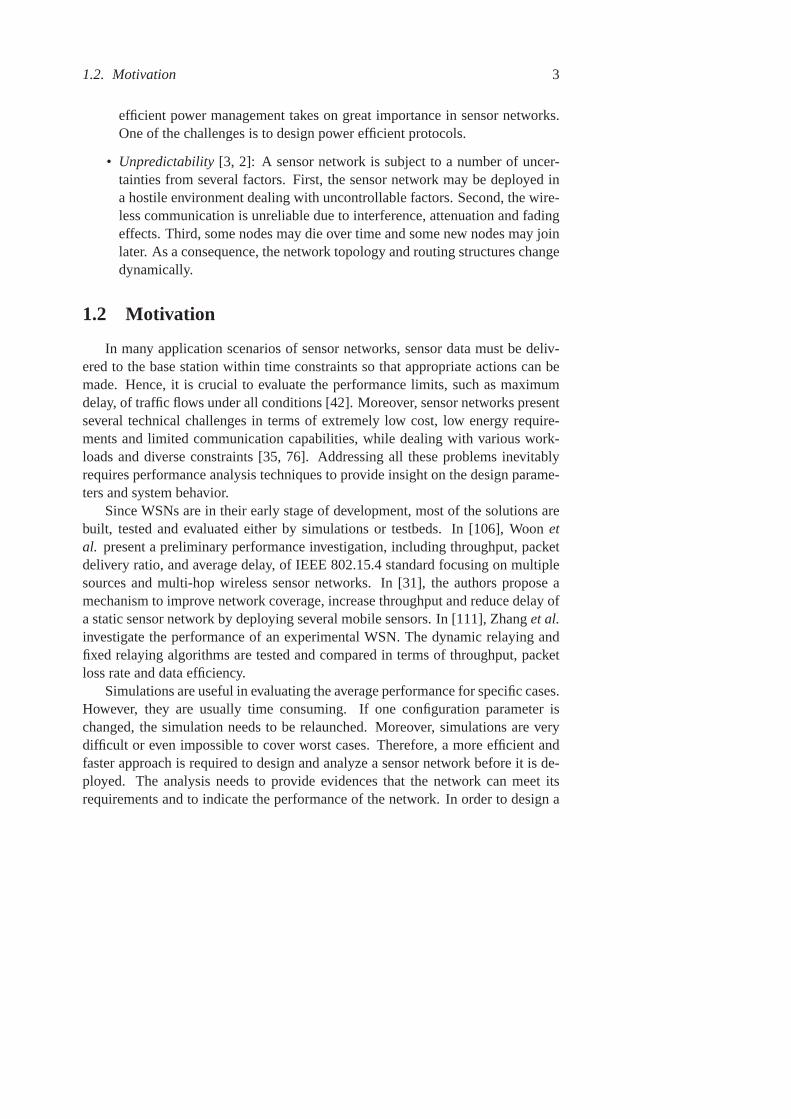
3.4 Modeling of Rayleigh Fading Channel . . . . . . . . . . . . . . . 543.4.1 Channel Model . . . . . . . . . . . . . . . . . . . . . . . 543.4.2 Stochastic Service Curve . . . . . . . . . . . . . . . . . . 563.4.3 Performance Bounds . . . . . . . . . . . . . . . . . . . . 563.4.4 Performance Evaluation . . . . . . . . . . . . . . . . . . 59
3.5 Bandwidth Estimation through Backlog Measurement . . . . . . . 663.5.1 Preliminaries . . . . . . . . . . . . . . . . . . . . . . . . 663.5.2 Backlog-Based Bandwidth Estimation . . . . . . . . . . . 693.5.3 Experimental Results . . . . . . . . . . . . . . . . . . . . 71
3.6 Summary . . . . . . . . . . . . . . . . . . . . . . . . . . . . . . 75
4 Coverage and Deployment 774.1 Introduction . . . . . . . . . . . . . . . . . . . . . . . . . . . . . 774.2 Related Work . . . . . . . . . . . . . . . . . . . . . . . . . . . . 794.3 Probabilistic Event Coverage . . . . . . . . . . . . . . . . . . . . 80
4.3.1 System Model . . . . . . . . . . . . . . . . . . . . . . . 804.3.2 Area Coverage . . . . . . . . . . . . . . . . . . . . . . . 814.3.3 Event Coverage . . . . . . . . . . . . . . . . . . . . . . . 834.3.4 Boundary Analysis . . . . . . . . . . . . . . . . . . . . . 844.3.5 Probabilistic Event Coverage in Heterogeneous Networks 864.3.6 Experimental Results . . . . . . . . . . . . . . . . . . . . 90
4.4 Deployment Strategies . . . . . . . . . . . . . . . . . . . . . . . 964.4.1 Definitions and Models . . . . . . . . . . . . . . . . . . . 984.4.2 Sensing and Coverage Model . . . . . . . . . . . . . . . 994.4.3 Coverage Analysis . . . . . . . . . . . . . . . . . . . . . 1004.4.4 Lifetime Analysis . . . . . . . . . . . . . . . . . . . . . . 1034.4.5 Cost Analysis . . . . . . . . . . . . . . . . . . . . . . . . 1044.4.6 Evaluation Results . . . . . . . . . . . . . . . . . . . . . 105
4.5 Summary . . . . . . . . . . . . . . . . . . . . . . . . . . . . . . 108
5 Summary and Future Work 1115.1 Summary . . . . . . . . . . . . . . . . . . . . . . . . . . . . . . 1115.2 Future Work . . . . . . . . . . . . . . . . . . . . . . . . . . . . . 112
References 115

List of Tables
2.1 System Parameters . . . . . . . . . . . . . . . . . . . . . . . . . 332.2 Experimental Parameters . . . . . . . . . . . . . . . . . . . . . . 46
4.1 Variables and Descriptions . . . . . . . . . . . . . . . . . . . . . 1014.2 Parameters . . . . . . . . . . . . . . . . . . . . . . . . . . . . . . 1054.3 Lifetime . . . . . . . . . . . . . . . . . . . . . . . . . . . . . . . 107
ix

x

List of Figures
1.1 A wireless sensor network for volcanic monitoring . . . . . . . . 2
2.1 (a): arrive curve and service curve; (b): delay bound and backlogbound . . . . . . . . . . . . . . . . . . . . . . . . . . . . . . . . 12
2.2 A cluster-mesh sensor network . . . . . . . . . . . . . . . . . . . 162.3 Energy per bit vs. transmission rate [74]:W = 20 kHz, N0 =
−100 dB, G0 = −50 dB, d = 5m, θ = 3. . . . . . . . . . . . . 182.4 (a) An affine arrival curve: the arrows show the packet generation
process; (b) A rate-latency service curve. . . . . . . . . . . . . . . 192.5 (a) The main flowf1 is split into two subflowsf1.1 andf1.2; (b)
The equivalent model. . . . . . . . . . . . . . . . . . . . . . . . . 212.6 (a) A node serves two input flows; (b) The equivalent model. . . . 232.7 An example of splitting strategies.s1 is the source node of the traf-
fic flow ands6 is the sink. (a) Flow based traffic splitting strategy;(b) Node based traffic splitting strategy. . . . . . . . . . . . . . . 25
2.8 (a) A network analysis example: the main flowf1 is split into twosubflowsf1.1 andf1.2. f2 is the contention flow; (b) The equivalentanalysis network: the blue, green, and red dashed lines show therouting path of flowf1.1, f1.2 andf2 respectively. . . . . . . . . . 27
2.9 A cluster-mesh sensor network:s0 is the sink. An event happensin the blue circle and three traffic flowsf1, f2, f3 are generated. . 32
2.10 (a) General routing with no splitting (NOS): the tagged main flowf1 chooses one of path 1, 2 or 3, and the routing paths off2 andf3are shown by the blue and green line respectively; (b) Flow basedsplitting (FBS): all three flows are split as shown by the red, blueand green lines respectively. . . . . . . . . . . . . . . . . . . . . 33
2.11 End-to-end least upper delay bound . . . . . . . . . . . . . . . . 342.12 Least upper backlog bounds (In NOS: flow 1 chooses path 3). . .. 35
xi

xii List of Figures
2.13 Variance of least upper backlog bounds (In NOS: flow 1 choosespath 3). . . . . . . . . . . . . . . . . . . . . . . . . . . . . . . . 35
2.14 Power consumption (In NOSi: flow 1 chooses pathi, wherei =1, 2, 3). . . . . . . . . . . . . . . . . . . . . . . . . . . . . . . . 36
2.15 Variance of power consumption. . . . . . . . . . . . . . . . . . . 362.16 End-to-end delay. . . . . . . . . . . . . . . . . . . . . . . . . . . 372.17 Least upper backlog bounds (In NOS: flow 1 chooses path 3). . .. 372.18 Variance of least upper backlog bounds (In NOS: flow 1 chooses
path 3). . . . . . . . . . . . . . . . . . . . . . . . . . . . . . . . 372.19 Power consumption (In NOSi: flow 1 chooses pathi, wherei =
1, 2, 3). . . . . . . . . . . . . . . . . . . . . . . . . . . . . . . . 382.20 Variance of power consumption. . . . . . . . . . . . . . . . . . . 382.21 Compare the end-to-end delay computed by two methods. . . . . 392.22 End-to-end delays in NOS. . . . . . . . . . . . . . . . . . . . . . 402.23 End-to-end delays in FBS. . . . . . . . . . . . . . . . . . . . . . 402.24 Nodes’ backlogs in NOS. . . . . . . . . . . . . . . . . . . . . . . 402.25 Nodes’ backlogs in FBS. . . . . . . . . . . . . . . . . . . . . . . 402.26 (a): Hop-by-hop retransmission; (b): End-to-end retransmission. . 432.27 Compare the maximum transmission delay . . . . . . . . . . . . . 472.28 Compare the energy consumption . . . . . . . . . . . . . . . . . 472.29 Compare analytical maximum transmission delay with the simula-
tion results . . . . . . . . . . . . . . . . . . . . . . . . . . . . . . 48
3.1 System model of a fading channel. . . . . . . . . . . . . . . . . . 553.2 Simulation results: delay. . . . . . . . . . . . . . . . . . . . . . . 603.3 Compare simulation and analytical results. . . . . . . . . . . . . . 613.4 Compare simulation results with analytical results: Markov arrivals. 623.5 Delay bound under different SNR and transmission data rates. . . 633.6 Violation probability of the delay and backlog bounds. . . . . . . 633.7 Violation probability of the delay and backlog bounds. . . . . . . 653.8 The delay bound. . . . . . . . . . . . . . . . . . . . . . . . . . . 653.9 Violation probability of the delay and backlog bounds. . . . . . . 663.10 Procedure of the bandwidth estimation method . . . . . . . . . . 693.11 Service rate of Rayleigh channel . . . . . . . . . . . . . . . . . . 713.12 Maximum backlog for different probing rates. . . . . . . . . . . . 723.13 Comparison of reference service curve and estimated service curve:
in simulation trials, the probe packet trains are sent with variousrates and the backlog bounds are measured. The thin dashed bluelines represent the results of bandwidth estimation from all the trials. 73

List of Figures xiii
3.14 Comparison of reference service curve and estimated service curvewith various channel parameters: 1) channel bandwidth; 2) meanof the received signal power (in Watt). . . . . . . . . . . . . . . . 74
3.15 Comparison of reference service curve and estimated service curvewith various inter-packet interval and packet length. . . . . . . . . 75
4.1 Left: area coverage; right: event coverage . . . . . . . . . . . . . 784.2 Left: heterogeneous sensor networks; right: homogeneous sensor
networks . . . . . . . . . . . . . . . . . . . . . . . . . . . . . . . 794.3 Boundary analysis . . . . . . . . . . . . . . . . . . . . . . . . . . 844.4 Coverage overlap . . . . . . . . . . . . . . . . . . . . . . . . . . 884.5 Probability of event coverage: 1-coverage . . . . . . . . . . . . . 904.6 Probability of event coverage: 2-coverage . . . . . . . . . . . . . 914.7 Probability of event coverage with different values ofk (λ = 0.3) 924.8 Event coverage probabilities in two-sub-FoI networks ( event den-
sity γ = 0.03, 0.06). ’hom’ denotes homogeneous deployment;’het’ denotes heterogeneou deployment; ’ovl’ means ’overlapping’between adjacent sub-FoIs are considered. . . . . . . . . . . . . . 93
4.9 Comparison of the event coverage probabilities of homogeneousand heterogeneous sensor deployments in two-sub-FoI networks(γ1 = 0.03, γ2 are changed) . . . . . . . . . . . . . . . . . . . . 94
4.10 Comparisons of the event coverage probabilities in multi-sub-FoInetworks . . . . . . . . . . . . . . . . . . . . . . . . . . . . . . . 94
4.11 Boundary analysis (γ = 0.03) . . . . . . . . . . . . . . . . . . . 954.12 Relative error of boundary analysis(γ = 0.03) . . . . . . . . . . . 964.13 System Architecture. . . . . . . . . . . . . . . . . . . . . . . . . 984.14 Uniform random . . . . . . . . . . . . . . . . . . . . . . . . . . 994.15 Rectangle mesh . . . . . . . . . . . . . . . . . . . . . . . . . . . 994.16 k-coverage map. . . . . . . . . . . . . . . . . . . . . . . . . . . . 1004.17 k-coverage map for calculation . . . . . . . . . . . . . . . . . . . 1004.18 The average k-coverage and variance. . . . . . . . . . . . . . . . 106

xiv

List of Abbreviations
ACK ACKnowledgmentARQ Automatic Repeat reQuestATM Asynchronous Transfer ModeBER Bit Error RateCSI Channel State IndicatorCSMA Carrier Sense Multiple AccessDNC Deterministic Network CalculusETS Even Traffic Splitting mechanismFBS Flow Based SplittingFIFO First-In-First-OutFoI Field of InterestMAC Medium Access ControlNACK Negative ACKnowledgmentNOS General routing with No SplittingPAN Personal Area NetworkPSFQ Pump Slowly and Fetch QuicklyPTS Probabilistic Traffic Splitting mechanismQoS Quality of ServiceRFID Radio-Frequency IDentificationRN Relay NodeRx ReceivingSN Sensor NodeSNC Stochastic Network CalculusSNR Signal-to-Noise-RatioTDMA Time Division Multiple AccessTx TransmissionWFP Wait for First PacketWSN Wireless Sensor NetworkWTS Weighted Traffic Splitting mechanism
xv

xvi

List of Publications
Articles
• Huimin She, Zhonghai Lu, Axel Jantsch, Li-Rong Zheng, "ProbabilisticEvent Coverage in Heterogeneous Sensor Networks", submitted to ACMTransactions on Sensor Networks, 2012.
• Huimin She, Zhonghai Lu, Axel Jantsch, Dian Zhou, Li-Rong Zheng, "Per-formance Analysis of Flow Based Traffic Splitting Strategy on Cluster-MeshSensor Networks",International Journal of Distributed Sensor Networks,Volume 2012, no-232937, 2012.
• Huimin She, Zhonghai Lu, Axel Jantsch, Li-Rong Zheng, Dian Zhou, "Anal-ysis of Traffic Splitting Mechanisms for 2D Mesh Sensor Networks",In-ternational Journal of Software Engineering and Its Applications (IJSEIA),Vol.2 No.3, July 2008.
In Proceedings
• Huimin She, Zhonghai Lu, Axel Jantsch, "System-Level Evaluation of Sen-sor Networks Deployment Strategies: Coverage Lifetime and Cost",the 8thInternational Wireless Communications and Mobile Computing Conference(IWCMC’2012), Cyprus, August 2012.
• Huimin She, Zhonghai Lu, Axel Jantsch, Li-Rong Zheng, "Estimation ofStatistical Bandwidth through Backlog Measurement",Workshop on Net-work Calculus (WoNeCa’2012), in conjunction with MMB&DFT 2012, Ger-many, March 2012.
xvii

xviii List of Publications
• Huimin She, Zhonghai Lu, Axel Jantsch, Dian Zhou, Li-Rong Zheng, "Stochas-tic Coverage in Event-Driven Sensor Networks",the 22nd IEEE Interna-tional Symposium on Personal, Indoor and Mobile Radio Communications(PIMRC’2011), Canada, September 2011.
• Huimin She, Zhonghai Lu, Axel Jantsch, Dian Zhou, Li-Rong Zheng, "Mod-eling and Analysis of Rayleigh Fading Channels using Stochastic NetworkCalculus", the IEEE Wireless Communication and Networking Conference(WCNC’2011), Mexico, April 2011.
• Huimin She, Zhonghai Lu, Axel Jantsch, Li-Rong Zheng, Dian Zhou, "Ana-lytical Evaluation of Retransmission Schemes in Wireless Sensor Networks",IEEE 69th Vehicular Technology Conference (VTC2009-Spring), Spain, April2009.
• Huimin She, Zhonghai Lu, Axel Jantsch, Li-Rong Zheng, Dian Zhou, "De-terministic Worst-case Performance Analysis for Wireless Sensor Networks",IEEE International conference on Wireless Communications and Mobile Com-puting (IWCMC’08), Greece, August 2008
• Huimin She, Zhonghai Lu, Axel Jantsch, Li-Rong Zheng and Dian Zhou,"Traffic Splitting with Network Calculus for Mesh Sensor Networks,"inProc. of IEEE conference on Future Generation Communication and Net-working (FGCN’07), volume 2, South Korea, December 2007.
Others
• Huimin She, Zhonghai Lu, Axel Jantsch, "WSN-Dim: Methodology forDimensioning and Planning of Wireless Sensor Networks",Poster in ICES4th Annual Conference: New Businesses based on Embedded Systems- Howto Succeed!, Sweden, September 2011
• Huimin She, Zhonghai Lu, Axel Jantsch, "Stochastic Coverage Analysisof Event-Driven Sensor Networks",in Proceedings of The Second NordicWorkshop on System and Network Optimization for Wireless (SNOW’2011),Sweden, March 2011

xix
• Huimin She, Zhonghai Lu, Axel Jantsch, Li-Rong Zheng, Dian Zhou, "Anetwork-based system architecture for remote medical applications",the 24thAsia-Pacific Advanced Network (APAN’07), China, August 2007.

xx

Chapter 1
Introduction
This chapter provides a brief background and outlines the design challenges inwireless sensor networks. It also gives an overview of the researchpresented in thethesis and highlight the author’s contributions.
1.1 Background
With the development of wireless communications and micro-electronics,wire-less sensor network(WSN) has become a promising technology and received sig-nificant research attention in recent years [73, 2, 65, 21, 50, 27, 105, 68].
A typical sensor network consists of a large number of sensor nodes deployedeither inside the phenomenon of interest or close to it. These sensor nodesaredevices equipped with sensing, computation, and wireless communication capabil-ities. They take measurements and forward their observation values via the wirelessinterfaces to single or multiple fusion centers, which can also be called a sink node.Typical sensing tasks for sensors could be temperature, light, humidity, vibration,sound, etc. There are a variety of WSNs applications, which typically involvemonitoring, tracking and controlling. Specific applications include environmentsurveillance, next-generation health-care systems, structural monitoring, supplychain management, disaster area monitoring, and military assistance [34, 3, 27].Figure 1.1 shows an application of sensor networks for volcanic monitoring[104].When an earthquake or an eruption occurs, sensor nodes detect the seismic eventand send data to a base station via a multi-hop network. Collecting and analyzingdata from multiple base stations can produce precise mappings of the volcano.
1

2 Chapter 1. Introduction
Figure 1.1. A wireless sensor network for volcanic monitoring
Although WSNs share many commonalities with existing ad hoc networks,there are still a number of unique features and application requirements [3,50, 27].These features, which are stated below, make the design of WSNs challenging.
• Application specific[10]: Sensor networks can be deployed in a variety ofapplication scenarios. It is unlikely that there will be one all-purpose solutionfor all the potential possibilities. Therefore, it is essential to design a sensornetwork that can meet the requirements and constraints of specific domains.
• Constrained resource[27]: Unlike traditional networks, sensor networks arelimited in power, computational capability and communication bandwidth.New solutions are needed both to meet the requirements of a specific appli-cation and to balance the trade-offs between performance and cost. On theother hand, in order to allocate the limited resource, evaluating the perfor-mance of WSNs is therefore a crucial task.
• Limited memory size[78]: Too much memory space would increase the costand size of sensors, while too little memory space can not meet the require-ments of applications. Hence, it is essential to estimate the required memoryspaces before the deployment of sensor networks.
• Low power requirements[75, 16]: Due to size and cost constraints, the tinysensor nodes can only be equipped with a limited power source. Moreover, insome application scenarios, recharge of power source is impossible. Hence,
1.2. Motivation 3
efficient power management takes on great importance in sensor networks.One of the challenges is to design power efficient protocols.
• Unpredictability [3, 2]: A sensor network is subject to a number of uncer-tainties from several factors. First, the sensor network may be deployedina hostile environment dealing with uncontrollable factors. Second, the wire-less communication is unreliable due to interference, attenuation and fadingeffects. Third, some nodes may die over time and some new nodes may joinlater. As a consequence, the network topology and routing structures changedynamically.
1.2 Motivation
In many application scenarios of sensor networks, sensor data must be deliv-ered to the base station within time constraints so that appropriate actions can bemade. Hence, it is crucial to evaluate the performance limits, such as maximumdelay, of traffic flows under all conditions [42]. Moreover, sensor networks presentseveral technical challenges in terms of extremely low cost, low energy require-ments and limited communication capabilities, while dealing with various work-loads and diverse constraints [35, 76]. Addressing all these problemsinevitablyrequires performance analysis techniques to provide insight on the design parame-ters and system behavior.
Since WSNs are in their early stage of development, most of the solutions arebuilt, tested and evaluated either by simulations or testbeds. In [106], Woonetal. present a preliminary performance investigation, including throughput, packetdelivery ratio, and average delay, of IEEE 802.15.4 standard focusing on multiplesources and multi-hop wireless sensor networks. In [31], the authors propose amechanism to improve network coverage, increase throughput and reduce delay ofa static sensor network by deploying several mobile sensors. In [111],Zhanget al.investigate the performance of an experimental WSN. The dynamic relaying andfixed relaying algorithms are tested and compared in terms of throughput, packetloss rate and data efficiency.
Simulations are useful in evaluating the average performance for specificcases.However, they are usually time consuming. If one configuration parameter ischanged, the simulation needs to be relaunched. Moreover, simulations areverydifficult or even impossible to cover worst cases. Therefore, a more efficient andfaster approach is required to design and analyze a sensor network before it is de-ployed. The analysis needs to provide evidences that the network can meet itsrequirements and to indicate the performance of the network. In order to design a

4 Chapter 1. Introduction
WSN with predictable delay, backlog and energy consumptions, formal methodsare desired to dimension sensor networks in an analytical way rather than case-by-case simulations. Starting with the seminal work by Cruz [25, 26],networkcalculushas been developed as a powerful tool for the performance analysis ofnetworked system [11, 44, 46] . In contrast to queueing theory, network calcu-lus deals with performance bounds, such as worst-case delay and backlog bounds,rather than average values. In general, network calculus has been developed alongtwo tracks:deterministic network calculus (DNC)andstochastic network calculus(SNC). The DNC generally considers the worst-case performance analysis throughdeterministic arrival curve and service curve. Recently, it has been extended andapplied for worst-case performance analysis of sensor networks by several re-searchers [81, 51, 82, 49]. To incorporate non-deterministic serviceprovisioning,the performance bounds have to be complemented with certain violation probabil-ities. SNC is such a tool that can be employed in the design of wireless networksto provide stochastic service guarantees. It has been applied to QoS analysis forwireless networks by many researchers recently [95, 45, 22, 60, 47].
WSNs generally have two fundamental application scenarios: tracking andmonitoring. In both applications, it is essential to ensure that information of thetarget or the environment can be discovered and collected by sensors.To achievegood coverage, sensors are usually densely deployed. One of the most popularmetrics to quantify the coverage performance is thek-coverage[43, 113]. An FoI(Field of Interest) is said to be k-covered if every point in it is covered byat leastk sensors. The coverage problem can be classified in different ways dependingon the way of sensor deployment and the features of applications. Moreover, thelifetime of WSN is determined by the energy budgets of sensors. To obtain longernetwork lifetime, more energy budgets should be assigned to sensors. Since sen-sors are usually equipped with batteries which are limited and expensive resources,deploying spare sensor nodes would cause high installation and maintenance cost.Therefore, in order to deploy minimum necessary sensors that can achieve the re-quirements, it is important to evaluate these performance metrics of a WSN beforeits deployment.
Performance analysis such as coverage, connectivity, energy consumption, costfor sensor networks has been studied by many researchers. In [20], the authors pro-posed a general framework for the analysis of the network lifetime and costs forseveral network deployment strategies in sensor networks. They investigated de-ployment strategies to maximize the network lifetime by mitigating the hot-spottraffic problem around the data sink. The coverage problem in sensor networkshas been extensively investigated [59, 112, 100, 52, 6, 8, 72, 115, 108]. Zhang

1.2. Motivation 5
and Hou [112] studied the problem of deriving the node density for maintainingk-coverage for a given network area in both random and deterministic deploymentstrategies. However, most attentions focused on analyzing the minimum coverage.In [88], the authors proposed an analytical method to model the event coverageproblem in sensor networks. In [72], the authors investigated the coverage, energyconsumption and message transfer delay of large-scale WSNs. They consideredthe square grid based deployment scheme which shows very good coverage perfor-mance and the Tri-Hexagon Tiling (THT) deployment strategy, which outperformsother schemes for energy consumption and worst-case delay.
Network calculus is a mathematical tool dealing with performance guaranteesin packet switching networks [25, 26, 17, 11, 44]. With the abstraction ofar-rival curve for traffic flows andservice curvefor network elements, it has beenwidely applied in communication networks for performance analysis. In general,network calculus has been developed in two tracks: deterministic network calculus(DNC) and stochastic network calculus (SNC). The DNC generally considers theworst-case performance analysis through deterministic arrival curve and servicecurve. Recently, it has been extended and used for worst-case performance analy-sis of sensor networks by several researchers [81, 51]. Since data communicationin wireless networks is unstable and irregular, it is very difficult or impossible tofind the deterministic performance bounds. To incorporate nondeterministic ser-vice provisioning, the performance bounds have to be complemented with certainviolation probabilities. SNC is such a tool which can be employed in the design ofwireless networks to provide stochastic service guarantees.
In this thesis, the research has been orienting in two tracks: performanceanal-ysis for WSNs using network calculus, and deployment mechanisms especiallycoverage analysis in WSNs.

6 Chapter 1. Introduction
1.3 Contributions and Outline
The remainder of this thesis is structured as follows:
Chapter 2
In this chapter, we present a deterministic analysis method integrating trafficsplitting and traffic multiplexing for worst-case performance analysis in WSNs.Moreover, two retransmission schemes are analytically evaluated: hop-by-hop re-transmission and end-to-end retransmission. Most of the materials were publishedin:
• Huimin She, Zhonghai Lu, Axel Jantsch, Dian Zhou, Li-Rong Zheng, "Per-formance Analysis of Flow Based Traffic Splitting Strategy on Cluster-MeshSensor Networks",International Journal of Distributed Sensor Networks,Volume 2012, no-232937, 2012.
Author’s contributions:The author developed the algorithm, implementedthe experiments and wrote the manuscript.
• Huimin She, Zhonghai Lu, Axel Jantsch, Li-Rong Zheng and Dian Zhou,"Deterministic Worst-case Performance Analysis for Wireless Sensor Net-works," in Proc. of the 2008 International conference on Wireless Com-munications and Mobile Computing Conference (IWCMC’08), Crete Island,Greece, August, 2008.
Author’s contributions:The author developed the algorithm, implementedthe experiments and wrote the manuscript.
• Huimin She, Zhonghai Lu, Axel Jantsch, Li-Rong Zheng, Dian Zhou, "Ana-lytical Evaluation of Retransmission Schemes in Wireless Sensor Networks",IEEE 69th Vehicular Technology Conference (VTC2009-Spring), Spain, April2009.
Author’s contributions:The author generated the ideas, developed the algo-rithm, implemented the experiments and wrote the manuscript.
Chapter 3
This chapter summarizes our research on applying stochastic network calculusfor wireless channel modeling, and bandwidth estimation through backlog mea-surement. We propose a network calculus based approach for Quality ofService(QoS) analysis of wireless channels subject to Rayleigh fading. Furthermore, a

1.3. Contributions and Outline 7
detailed mechanism for bandwidth estimation of random wireless channels basedon stochastic network calculus is developed. The bandwidth is derived from themeasurement of statistical backlogs based on probe packet trains. The theoreticfoundation and the detailed step-by-step procedure of the estimation method arealso presented.
Part of the results were published in:
• Huimin She, Zhonghai Lu, Axel Jantsch, Dian Zhou, Li-Rong Zheng, "Mod-eling and Analysis of Rayleigh Fading Channels using Stochastic NetworkCalculus", the IEEE Wireless Communication and Networking Conference(WCNC’2011), Mexico, April 2011.
Author’s contributions:The author contributed with the idea, solution, ex-periments and wrote the manuscript.
• Huimin She, Zhonghai Lu, Axel Jantsch, Li-Rong Zheng, "Estimation ofStatistical Bandwidth through Backlog Measurement",Workshop on Net-work Calculus (WoNeCa2012), in conjunction with MMB&DFT 2012, Ger-many, March 2012.
Author’s contributions:The author developed the algorithms, conducted theexperiments and wrote the manuscript.
Chapter 4
This chapter contains the research on coverage analysis and deployment mech-anisms in WSNs. A probabilistic event coverage analysis method is proposedforevaluating the coverage performance of heterogeneous sensor networks with ran-domly deployed sensors and stochastic event occurrences. Moreover, we introducetechniques for analyzing the coverage, network lifetime and cost both in randomdeployed and regular sensor networks.
Part of the results were published in:
• Huimin She, Zhonghai Lu, Axel Jantsch, Dian Zhou, Li-Rong Zheng, "Stochas-tic Coverage in Event-Driven Sensor Networks",the 22nd IEEE Interna-tional Symposium on Personal, Indoor and Mobile Radio Communications(PIMRC’2011), Canada, September 2011.
Author’s contributions:The author contributed with the idea, solution, ex-periments and wrote the manuscript.
An extended version of the conference paper is submitted to:

8 Chapter 1. Introduction
• Huimin She, Zhonghai, Axel Jantsch, Li-Rong Zheng, "Probabilistic EventCoverage in Heterogeneous Sensor Networks", submitted to ACM Transac-tions on Sensor Networks, 2012.
Author’s contributions:The author contributed with the idea, solution, ex-periments and wrote the manuscript.
• Huimin She, Zhonghai, Axel Jantsch, "System-Level Evaluation of SensorNetworks Deployment Strategies: Coverage Lifetime and Cost",the 8th In-ternational Wireless Communications and Mobile Computing Conference(IWCMC’2012), Cyprus, August 2012.
Author’s contributions:The author contributed with the idea, solution, ex-periments and wrote the manuscript.
Chapter 5
This chapter summarizes the thesis and proposes several open topics forfutureinvestigation.

Chapter 2
Deterministic PerformanceAnalysis
In this chapter, we present a deterministic analysis method integrating trafficsplitting and traffic multiplexing for worst-case performance analysis in WSNs.Moreover, two retransmission schemes are analytically evaluated: hop-by-hop re-transmission and end-to-end retransmission. The work in this chapter is mainlybased on [83, 84, 85, 90, 86].
2.1 Introduction
A typical sensor network consists of a larger number of sensor nodes that arecapable of sensing the environment and forwarding their observation values to afusion center (sink) through multi-hop wireless links. Thus, the traffic pattern insensor networks is usually in a many-to-one manner. The nodes near the sink mayneed to forward more data and thus consume more energy and buffer thanthe nodesfar away. Consequently, the distributions of energy and buffer requirements inWSNs might be extremely uneven. Unfortunately, energy supplies and buffers arelimited and expensive resources in typical WSNs, since sensor nodes are usuallymade as tiny devices with limited buffers and equipped with batteries that may notbe convenient or economical for replacement. One way to address thesechallengesis applying traffic splitting strategies which have been adopted by many researchersfor load balancing in communication networks [97, 66]. With traffic splitting, amain flow is divided into several subflows and forwarded to the destination throughdifferent routing paths. By distributing traffic over the network, the overall networkload balance can be improved. It is shown in [109] that the spare capacitycan
9

10 Chapter 2. Deterministic Performance Analysis
be reduced and thus the overall performance of the system can be improved bysplitting traffic across multiple disjoint paths.
One popular application of WSNs is real-time monitoring and tracking, suchas logistic chain tracking [114] and health-care application [40]. In suchkind ofapplications, it is crucial to ensure sensor data delivered to the sink within timeconstraints so that appropriate actions can be made. In order to design a WSN withpredictable delay, backlog and energy consumptions, formal performance analy-sis is desired for analyzing a sensor network before its actual deployment. Whilesimulation running based methods can offer high accuracy, it can be verytime-consuming and tedious to find the worst-case performance. Each simulation maytake considerable time and evaluates only a single network configuration, trafficpattern, and load point. Hence, formal methods are desired to dimension sensornetworks in an analytical way rather than case-by-case simulations. Starting withthe seminal work by Cruz [25, 26],network calculushas been developed as a pow-erful tool for the performance analysis of networked system [11]. Incontrast toqueueing theory, network calculus deals with performance bounds, such as worst-case delay and backlog bounds, rather than average values. It has been applied tosensor networks by many researchers recently [81, 51, 82, 49].
Data transmission in WSNs is unreliable due to several factors such as fading,shadowing and multi-path effects of radio propagation. One of the most commonapproaches for enhancing transmission reliability is retransmission [71, 99, 69].Parket al. [71] propose a scalable framework for reliable downstream data de-livery using aWait-for-First-Packet (WFP)pulse. In [99], Wanet al. propose areliable transport protocol called PSFQ(Pump Slowly and Fetch Quickly). Thesetwo protocols are typical examples that make use of hop-by-hop retransmissions.In [69], Paiet al. present an adaptive retransmission mechanism which allows afusion center to select the sensors to retransmit their local information accordingto the reliability of the received information. This protocol belongs to end-to-endretransmission.
In this chapter, an analytical method for the performance analysis of WSNsbased on deterministic network calculus is presented. Section 2.4 contains theanalysis of traffic splitting strategies for mesh sensor networks. In Section2.5, amethod to analyze the retransmission schemes is presented.
2.2 Related Work
In general packet switching networks, network calculus provides methods todeterministically reason about timing properties and resource requirements.Based

2.2. Related Work 11
on the powerful abstraction ofarrival curve for traffic flows andservice curvefornetwork elements, it allows computing the worst-case delay and backlog bounds.Systematic introduction of network calculus can be found in books [11, 17].
Network calculus has been extremely successful for ensuring performance boundswhen it is applied to Asynchronous Transfer Mode (ATM), Internet, and other net-works. It has been recently extended and applied for performance analysis andresource dimensioning of WSNs by several researchers. In [81], Schmitt et al.firstly applied network calculus to sensor network and proposed a generic frame-work for performance analysis of WSNs with various traffic patterns. They furtherextended the general framework to incorporate computational resources besides thecommunication aspects of WSNs [82]. In [51], Aniset al. proposed a methodol-ogy for the modeling and worst-case dimensioning of cluster-tree sensor networks.They derived plug-and-play expressions for the end-to-end delay bounds, buffer-ing and bandwidth requirements as a function of the WSN cluster-tree and trafficcharacteristics. Lenziniet al. [55] proposed a method for deriving tight end-to-end least upper delay boundsin sink-tree networks. The least upper delay boundis defined as the minimum value of the upper delay bound. In [49], the authorspresented a method for computing the worst-case delays, buffering and bandwidthrequirements while assuming that the sink node can be mobile.
Traffic splitting strategies have several common features with multi-path rout-ing protocols. There have been plenty of research works on multi-path routingand traffic splitting for sensor networks [36, 62, 61, 116, 56, 67]. The authors in[36] proposed a multi-path routing scheme that finds several disjoint paths. In thisscheme, the source node or an intermediate node chooses one path from the avail-able paths to deliver the data to sink based on the performance requirementssuchas delay and throughput. An energy efficient multi-path routing protocol for WSNswith multiple sinks is presented in [62]. The path construction is implemented bythe source node sending route messages to its neighbors. Traffic is distributed overthe multiple paths according to a load balancing algorithm. The results show thatthe proposed scheme results in a higher energy efficiency. In [61], authors proposedan N-to-1 multi-path routing protocol, in which nodes are arranged in a spanningtree. Multi-paths are constructed by traversing the tree. The multi-path scheme is acombination of end-to-end multi-path traffic dispersion and per-hop alternate pathsalvaging. Zouet al. [116] studied the interplay between data aggregation and flowsplitting in WSNs and proposed a flow-based scheme. The flows are preserved un-til the aggregation point. The aggregated data is splitted into multiple flows on therest of the path to the destination. The results show that the scheme can balance en-ergy consumption and therefore prolong the lifetime of WSNs. In [56], the authors

12 Chapter 2. Deterministic Performance Analysis
time
data (bits)
B(t)
D(t)
R(t)
R*(t)
time
data (bits)
R(t))(t
R*(t) )(t!
t t
(a) (b)
Figure 2.1. (a): arrive curve and service curve; (b): delay bound and backlog bound
investigated a joint coding/routing optimization of network costs and capacity inWSNs. By combining the link rate allocation and network coding-based multi-path routing, the total energy consumption of encoding power, transmissionpowerand reception power can be reduced. A back-pressure collection protocol (BCP)for sensor networks is presented in [67]. In this protocol, routing and forward-ing decisions are made based on a per-packet basis. By using ETX optimizationand floating LIFO queues, BCP is capable of improving throughput and deliveryperformance under static and dynamic settings, respectively.
2.3 Basics of Deterministic Network Calculus
Network calculus contains two parts, which are deterministic network calculus[25, 26, 11, 1] and stochastic network calculus [44]. In this chapter, the analysis isbased on deterministic network calculus. In general, network calculus is a min-plussystem theory for deterministic queuing systems [11]. It has been developed fordeterministic queuing, allowing to derive deterministic guarantees on throughputand delay, and bounds on buffer sizes. Specifically, network calculusanalyzes theworst-case behavior of a network rather than the average behavior.
Next, some basic definitions and notations are provided. Detailed definitionsand descriptions can be found in [11].
Definition 2.1 Min-Plus ConvolutionLet f(t) andg(t) bewide-sense increasingfunctions1 defined over real num-
bert ≥ 0, andf(0) = g(0) = 0. Then their convolution under min-plus algebra is
1A functionh is wide-sense increasing if and only ifh(s) ≤ h(t) for all s ≤ t.

2.3. Basics of Deterministic Network Calculus 13
defined as:(f ⊗ g)(t) = inf
0≤s≤t{f(t− s) + g(s)} (2.1)
An arrival process can be modeled by its cumulative trafficR(t), which isdefined as the number of bits that arrive in the time interval[0, t]. In particular,R(0) = 0 andR(t) is wide-sense increasing. Similarly, the output functionR∗(t)of a system is the number of bits that depart from the system in time interval[0, t].In particular,R∗(0) = 0 andR∗(t) is wide-sense increasing.
Definition 2.2 Arrival curveGiven a flow with input functionR(t), a wide-sense increasing functionα(t)
is an arrival curve forR(t) if and only if (Figure 2.1),
∀t ≥ 0, s ≥ 0 ands ≤ t : R(t)−R(t− s) ≤ α(s) (2.2)
One of the most commonly used arrival curve is theaffine arrival curve[11],which is defined as:
α(t) = ρ · t+ σ (2.3)
whereσ andρ represent the burst tolerance (in units of data) and the rate (in unitsof data per unit time), respectively. The average data rateρ gives an indication ofthe expected traffic volume in a given period of time. And burstinessσ describesthe maximum traffic above the average rate during any time interval.
Definition 2.3 Service CurveAssume that a server process is able to processS(t) bits of input data until time
t. Then, a wide-sense increasing functionβ(t) is a service curve forS(t) if andonly if (Figure 2.1),
∀t ≥ 0, 0 ≤ s ≤ t : S(t)− S(t− s) ≥ β(s) (2.4)
One of the most commonly used service curve is therate-latencyservice curve[11], which is defined as:
β(t) = R[t− T ]+ (2.5)
whereR represents the service data rate andT represents the maximum servicedelay. Ifx ≥ 0, notation[x]+ = x; otherwise it equals to 0.
With the arrival curve and service curve, the following theorems can be derivedbased on the network calculus theory. The detailed descriptions and proofs of thesetheorems can be found in [11].

14 Chapter 2. Deterministic Performance Analysis
Theorem 2.1Delay boundAssume a traffic flowR(t), constrained by arrival curveα(t), traverses a sys-
tem that provides a service curveβ(t). At any timet, the virtual delayD(t) satis-fies,
D(t) ≤ supt≥0
{ infτ≥0
{τ : α(t) ≤ β(t+ τ)}} (2.6)
The delay bound defines the maximum delay that would be experienced by abit arriving at timet. Graphically, the delay bound is the maximum horizontaldeviation betweenα(t) andβ(t) (Figure 2.1).
Theorem 2.2Backlog BoundAssume a traffic flowR(t), constrained by arrival curveα(t), traverses a sys-
tem that provides a service curveβ(t). The backlogB(t) for all t satisfies,
B(t) ≤ supt≥0
{α(t)− β(t)} (2.7)
The backlog is the amount of bits that are held inside the sensor node. The re-quired buffer size of a sensor node is determined by the maximum backlog. Graph-ically, the backlog bound is the maximum vertical deviation betweenα(t) andβ(t)(Figure 2.1).
Theorem 2.3Output boundAssume a traffic flowR(t), constrained by arrival curveα(t), traverses a sys-
tem that provides a service curveβ(t). The output flow is constrained by the fol-lowing arrival curve:
α∗(t) = sups≥0
{α(t+ s)− β(s)} (2.8)

2.4. Analysis of Traffic Splitting Scheme 15
Theorem 2.4ConcatenationAssume a flow sequentially traverses two systems which offer a service curve
of β1 andβ2, respectively. Then the concatenation of the two systems offers theflow the service curveβ(t), which is defined by,
β(t) = (β1 ⊗ β2)(t) = inf0≤s≤t
{β1(t− s) + β2(s)} (2.9)
where⊗ representsmin-plus convolution(Definition 2.1). Ifβ1 andβ2 are rate-latency service curves, i.e.β1(t) = R1[t − T1]
+ andβ2(t) = R2[t − T2]+, then
β1 ⊗ β2 = R∗[t− T ∗]+, whereR∗ = min(R1, R2) andT ∗ = T1 + T2.
Theorem 2.5Aggregate MultiplexingConsider a node multiplexing two flows 1 and 2 inFirst-In-First-Out (FIFO)
order. Assume that the node provides a guaranteed service curveβ(t) to the aggre-gate of the two flows and flow 2 is constrained by an arrival curveα2(t). Then, foranyθ ≥ 0 andt ≥ θ, flow 1 is guaranteed with the following service curve,
βθ1(t) = [β(t)− α2(t− θ)]+ (2.10)
This is also called leftover service, since it is the leftover capability of the nodeafter serving flow 2.
2.4 Analysis of Traffic Splitting Scheme
In this section, based on network calculus, we propose a flow based trafficsplitting strategy and an analytical method for worst-case performance analysis oncluster-mesh sensor networks. The traffic splitting strategy is useful in balancingnetwork load and power consumption. Aiming to evaluate the worst-case perfor-mance in terms of end-to-end least upper delay bound, least upper backlog boundand power consumption, a splitting model is built for a single node analysis andan analytical method is proposed for the network analysis. Through an example,it is shown that the performance analysis method is able to derive closed-form for-mulas of these bounds. The numerical results indicate that the backlog and powerconsumption can be balanced by applying the traffic splitting strategy. In addition,simulations are performed to validate the performance bounds of our analyticalmethod. The results show that their tightnesses are satisfactory.
2.4.1 System Model
This section presents system models, including the cluster-mesh network topol-ogy and power consumption model.

16 Chapter 2. Deterministic Performance Analysis
Sink
Sensor
Cluster
Head
Cluster
Figure 2.2. A cluster-mesh sensor network
A WSN may consist of a large number of sensors that are densely deployedeither inside the phenomenon of interest or close to it. These sensors can be orga-nized in various topologies, such as mesh and cluster based topologies. The meshnetworking has advantages like supporting path diversity which enables better bal-ance on traffic load and energy consumption [9]. The cluster based topologies arealso quite suitable for WSNs with demanding requirements in terms of Qualityof Service (QoS) support and real-time communications [51]. Consideringtheseaspects, we adopt thecluster-meshtopology that merges advantages of mesh andcluster [54, 70]. It is a two-layered architecture with the mesh defining a back-bone that consists of a set ofcluster heads(CH). A cluster is formed by groupinga number of sensors within a geographic neighborhood. We define the networkcomposed by cluster heads and the sink as the layer-1 network, and the networkinside a cluster as the layer-2 network.
In summary, the cluster-mesh network contains three types of nodes:sink, clus-ter headand sensor. Like in most sensor networks, the sink is responsible for con-trolling the network and collecting data from all the other nodes. A cluster headand multiple sensors form a cluster. In order to reduce the cost and complexity, sen-sors do not communicate with each other and data generated by them is collectedby their cluster head and delivered to the sink through neighbor cluster heads. Forsimplicity and conciseness, we consider cluster heads static and they do notsensethe environment nor generate input data. However, this assumption can beeas-ily relaxed and the subsequent analysis is straightforward. In the mesh networkcomposed by cluster heads and the sink, links are considered bidirectional.

2.4. Analysis of Traffic Splitting Scheme 17
Fig. 2.2 shows an example of the cluster-mesh topology. A cluster-mesh net-work is a mesh network where each cluster head and its connected sensors form itown logical cluster. The layer-1 network can be modeled as a direct graph G(N,L),whereN is the set of all sensor nodes and the sink andL is the set of all directlinks in the network. In this paper, our work concentrates on analyzing thelayer-1network.
In most types of sensor nodes, the energy consumption is mainly contributedbythe transmitter, receiver and computation module [75]. The application scenariosof sensor networks for fresh food monitoring in warehouses are considered. In thisscenario, sensors may perform tasks and send packets periodically. Consequently,the power consumption of the computation module can be considered as nearlyconstant denoted bypc. Let ǫr denote the energy consumption of the receiver elec-tronics for receiving one bit data. In practical applications, the power consumptionof the receiving is usually stable [75]. Soǫr can be considered as a constant. Ac-cording to the results in [74], the energy required to transmit a given amount ofdata is a convex and monotonically increasing function of the transmission rate,i.e., the energy per bit can be expressed as (Fig. 2.3),
ǫt =N0
RG
(2
RηW − 1
)(2.11)
whereR is the transmission rate,W is the channel bandwidth,G is the channelgain,N0 is the noise power, andη ∈ (0, 1) is the probability that the informationcan be reliably transmitted at a given transmission rate2. A simplified model forchannel gain is adopted, i.e.,G = G0(d/d0) (Section 2.6 of [37]), whereθ isthe path loss exponent(2 ≤ θ ≤ 4), d is the distance between the transmitterand receiver,d0 is a reference distance where the reference channel gainG0 ismeasured.
Therefore, the total power consumptionPi of a nodei can be expressed as,
Pi = ǫr∑
k∈Nin(i)
ρki +∑
j∈Nout(i)
ǫtijρij + pc
= ǫr∑
k∈Nin(i)
ρki +∑
j∈Nout(i)
ρijN0
RijGij
(2
RijηW − 1
)+ pc
(2.12)
whereρki andρij denote the data rates on linkki andij, respectively,Rij denotesthe transmission rate of nodei sending data to nodej, Gij = G0(dij/d0)
−θ de-notes the channel gain between nodei andj,Nin(i) denotes the set of nodes which
2In an optimal channel coding scheme, a transmission rateR = ηC can be guaranteed for any0 < η < 1, whereC = W log2(1 +GP/N0) is the Shannon capacity [74].

18 Chapter 2. Deterministic Performance Analysis
0 2 4 6 8 10
x 104
0
1
2
3
4
5
6x 10
−7 Energy per bit vs. transmission rate
Transmission rate (bit/s)
Ene
rgy
(J)
Figure 2.3. Energy per bit vs. transmission rate [74]:W = 20 kHz, N0 =−100 dB, G0 = −50 dB, d = 5 m, θ = 3.
are the direct sources of incoming data flows of nodei; Nout(i) denotes the set ofnodes which are the direct destinations of output data flows of nodei.
As stated in the previous section, sensor nodes inside a cluster generate inputdata and then send them to their cluster head. A trafficflow is defined as an infinitestream of data from a source to a destination. Following network calculus, theinput flow at a cluster head is modeled using its cumulative trafficR(t), defined asthe number of bits coming from the flow in time interval[0, t]. Furthermore, weuse a wide-sense increasing functionα(t) to constrain this cumulative traffic flowR(t), defined as
R(t)−R(s) ≤ α(t− s); ∀t ≥ 0, t ≥ s (2.13)
whereα(t) is called the arrival curve of the input flowR(t) [11]. Affine arrivalcurve is one of the most commonly used arrival curves, which has been adoptedin many works [81, 51, 82, 49]. The application scenario of this work is real-timemonitoring, the sensor nodes sense the environment and send packets periodicallyto the cluster heads. Therefore, the affine arrival curve model can be used to ab-stract the input traffic of cluster heads, defined asα(t) = γσ,ρ = ρ · t + σ, whereσ andρ represent the burst tolerance (in bits) and the average data rate (inbits/s),

2.4. Analysis of Traffic Splitting Scheme 19
respectively. Fig. 2.4-(a) shows examples of a periodic cumulative flowR(t) andan affine arrival curveα(t).
(a) (b)
time
data
slope = !
time
data
T
slop
e = R
(t)= t+!
Packet
!" ][)( TtRt#
Figure 2.4. (a) An affine arrival curve: the arrows show the packet generationpro-cess; (b) A rate-latency service curve.
Service curve is an abstraction to model the processing capability of a node,depending on link layer characteristics, such as transmission rate, channel charac-teristics, and packet scheduling. The node and the channel together are modeledas a network element which provides a service curveβs to the input flows. Ifthe node forwards packets with the rateR (bits/s) and delays packets forT (s)at maximum due to scheduling and queuing, it can be modeled by arate-latencyservice curve [11] that consists of two components: arate service curveand alatency service curve. The rate-latency service curve can be formally defined asβ(t) = χR,T = R[t− T ]+, where notation[x]+ denotesmax{0, x}.
In wireless networks, data transmission over wireless channels is usually unre-liable due to their inherent uncertainties. The actual transmission rate and successprobability are influenced by the transmission power, path loss, noise power and in-terference. In spite of these uncertainties, deterministic network calculus can stillbe useful in modeling wireless networks by making reasonable assumptions andabstractions. First, the uncertainties in some applications of WSNs are low. Anex-ample scenario for which our framework suits well is the process monitoring andtracking in logistics systems [114]. Second, the link unreliability and data loss ratecan be mitigated by applying high transmission powers, especially for the caseswith small distances between a transmitter and a receiver. Third, the interferencebetween adjacent nodes can be alleviated by using appropriate MAC layerproto-cols. There are plenty of research works on designing TDMA-based link protocolswhich can create collision-free slot schedules [33, 79].
Based on these assumptions about link reliability and interference, the service

20 Chapter 2. Deterministic Performance Analysis
capability of a node can be abstracted and approximated by a deterministic servicecurve with the idea of effective transmission rate. From information theory,theShannon capacity of a wireless channel can be expressed as,C = W log2(1 +GP/N0), whereW,G,N0 are the same as those in Eq. (2.11). The service rateis defined as the rate that the information can be reliably transmitted. With anoptimal or suboptimal channel coding scheme, a service rate ofR = η · C can beguaranteed for any0 < η < 1 [74]. R defines a lower bound on the transmissionrate. Therefore, the rate-latency service curveβ(t) = χR,T = R[t − T ]+ can beapplied to model the service capability of a wireless channel, whereT denotes themaximum possible processing/queueing delay.
Given the arrival curve and service curve of a node, the least upper delay bound,least upper backlog bound and output bounds can be derived according to networkcalculus [11]. The least upper backlog bound is defined as the minimum value ofthe upper backlog bound. Consider a nodei provides a service curveβs
i to the inputflow which is constrained by an arrival curveαi. According to network calculus ,the least upper delay bound of the flow can be computed by
Di = h(αi, βsi ) = sup
t≥0
{infτ≥0
{τ : αi(t) ≤ βsi (t+ τ)}
}. (2.14)
Moreover, the least upper backlog bound of nodei can be calculated by
Bi = v(αi, βsi ) = sup
t≥0{αi(t)− βs
i (t)} . (2.15)
Additionally, the arrival curve of the departure flow can be derived by
αi = αi ⊘ βsi = sup
τ≥0{αi(t+ τ)− βs
i (τ)} . (2.16)
2.4.2 Analysis
In this section, the splitting and multiplexing models are introduced. Then,the formal performance analysis procedure is presented. After that, thescope andassumptions of the analysis approach are discussed.
The Splitting Model
To analyze the splitting strategy, we build a splitting model that identifies therelations of input, output, delay and backlog for a single node. Without losinggenerality, a main flow is split into two subflows. The node thatf1 traverses isabstracted as the combination of a buffer plus asplitter depicted in Fig. 2.5-(a).

2.4. Analysis of Traffic Splitting Scheme 21
Consider that the node performs a weighted proportional splitting scheme, inwhich the main flow is split according to the configured weights,φi for subflowi. In each round, the splitter will try to forwardφi packets to output linki beforemoving to the next one. The values ofφi can be set either according to a pre-definedrule or randomly. Increasing the value ofφi can result in increased packets tooutput linki. By adjustingφi, the amount of traffic over each link can be controlled.If the service rate isR bits/s, the maximum length of a round is consequently equalto∑
i φil/R seconds and the time for packets of subflowi to be forwarded withina round is bounded byφil/R seconds, wherel is the packet length. In the weightedproportional splitting scheme, the worst case appears when the packets of a subflowjust misses its turn in the current round. Consequently, it will have to wait for itsturn at the next round. In the worst case, packets of the subflowi have to wait upto∑
i 6=j φjl/R seconds to be served.
(a)
1.1f
2.1f1f 1
2
s!FIFO
1.1f
2.1f
1f1
2
s
1!
s
2!
(b)
B1
B2
B
Figure 2.5. (a) The main flowf1 is split into two subflowsf1.1 andf1.2; (b) Theequivalent model.
Consider a main flowf1 that is upper constrained by arrival curveα1 = γσ1,ρ1 ,be split into two subflowsf1.1 andf1.2 according to weightsφ1 andφ2, whereσ1andρ1 denote the burstiness and average data rate off1, respectively. Burstinessis defined as the amount of data inputted/outputted to/from a system or a node atone time. Consequently, it should be equal or bigger than the packet sizel. Letα1.1 = γσ1.1,ρ1.1 andα1.2 = γσ1.2,ρ1.2 denote the arrival curves off1.1 andf1.2,respectively. Then,
ρ1.1 =φ1
φ1 + φ2ρ1, σ1.1 = max
(⌈φ1σ1
(φ1 + φ2)l
⌉· l, l)
(2.17)
ρ1.2 =φ2
φ1 + φ2ρ1, σ1.2 = max
(⌈φ2σ1
(φ1 + φ2)l
⌉· l, l)
(2.18)
where⌈·⌉ denotes the minimum integer equal to or bigger than the number inside.

22 Chapter 2. Deterministic Performance Analysis
Assume that the splitter provides a service curveβs = χR,T . Since the splitterserves one subflow at one time, the service rate for each subflow also equalsR.Therefore, the equivalent service curve for subflowf1.1 can be derived by
βs1 = βs ⊗ δφ2l
R
= χR,T+
φ2l
R
. (2.19)
Analogously, the equivalent service curve forf2.2 is
βs2 = βs ⊗ δφ1l
R
= χR,T+
φ1l
R
. (2.20)
Furthermore, the equivalent bounds on backlogs can be calculated by
B1 = σ1.1 +φ1ρ1
φ1 + φ2
(T1 +
φ2l
R
), B2 = σ1.2 +
φ2ρ1φ1 + φ2
(T1 +
φ1l
R
).(2.21)
Therefore, the least upper bound of the total backlog is computed by
B = B1 +B2 = σ1 + ρ1
[T +
2φ1φ2l
R(φ1 + φ2)
]. (2.22)
The least upper delay bounds consist of three parts: the processing time, thetime to serve input burstiness, and the scheduling delay. LetD1.1 andD1.2 denotethe delay bounds of subflowf1.1 andf1.2, respectively. They can be computed by
D1.1 = T +σ1.1R
+φ2l
RD1.2 = T +
σ1.2R
+φ1l
R. (2.23)
Furthermore, the departure arrival curves off1.1 andf1.2 can be derived by
α1.1 =φ1ρ1
φ1 + φ2t+ σ1.1 +
φ1
φ1 + φ2(ρ1T +
ρ1φ2l
R)
α1.2 =φ2ρ1
φ1 + φ2t+ σ1.2 +
φ2
φ1 + φ2(ρ1T +
ρ1φ1l
R). (2.24)
The Multiplexing Model
In order to analyze resource sharing when multiple input flows share the band-width of a link at a node, a multiplexing model is proposed. This model should beused for analyzing a network with various traffic flowing scenarios.
Without loss of generality, let us consider a node serve two flowsf1 andf2 inthe FIFO order as shown by Fig. 2.6-(a). And its equivalent model is drawn in Fig.2.6-(b). Let the node provide a service curveβs to the aggregating flows, andf1

2.4. Analysis of Traffic Splitting Scheme 23
andf2 haveα1 andα2 as arrive curves, respectively. We defineβs1 = κ(βs, α2) as
theequivalent service curve[55] provided to flowf1, whereκ(·, ·) is an operatorto compute the equivalent service andτ is an intermediate argument. Thus, thedeparture arrival curve off1 can be derived byα1 = α1 ⊘ κ(βs, α2), and its leastupper delay bound is computed byh(α1, κ(β
s, α2)), and the least upper backlogbound of the node isv(α{1,2}, β
s), whereα{1,2} denotes the arrival curve of theaggregating flowf{1,2}. Similarly, the equivalent service curve provides to flowf2can be derived byβs
2 = κ(βs, α1), and its delay and backlog bounds, and departurearrival curve can be derived accordingly.
(a)
s 1f
2f
FIFO1!
2!
*
1!
*
2!
(b)
1f
2f
1!
2!
*
1!
*
2!
s
1
s
2
B
Figure 2.6. (a) A node serves two input flows; (b) The equivalent model.
An example is given to show how to computeκ(·, ·). Let βs(t) = χR,T =R[t− T ]+, andα2(t) = γσ2,ρ2(t) = ρ2t+ σ2, then applying Corollary 4.5 in [55],the equivalent service curve forf1 can be calculated by
βs1 = κ(βs, α2) = γR·τ,R−ρ2 ⊗ δT+
σ2R
+τ (τ ≥ 0) (2.25)
whereτ is an intermediate argument for calculating the least upper delay bound,andδT (t) = +∞ for t > T , and0 otherwise.
The least upper delay bound off1 is calculated by
D1 = h(α1, βs1) = inf
τ≥0
{T +
σ2R
+σ1 −Rτ
R− ρ2+ τ
}. (2.26)
Furthermore, the least upper backlog bound of the node can be derived by
B = σ1 + σ2 + (ρ1 + ρ2)T. (2.27)
Additionally, the arrival curve of the departure flow off1 is computed by
α1 = α1 ⊘ βs1 = ρ1t+ σ1 + ρ1
(T +
σ2R
+ τ), (2.28)
whereτ is the same as the value obtained in equation (2.26).

24 Chapter 2. Deterministic Performance Analysis
The Splitting Based Performance Analysis Procedure
There have been several research works on the traffic splitting strategy in packetnetworks [66, 109], due to its efficiency in load balancing. In the flow basedsplitting strategy, a traffic flow is split into multiple subflows at its source node,and these subflows are forwarded to the sink through different routingpaths. Thesource node decides how the subflows are split. Given the traffic patterns, servicemodels, the routing protocols and the splitting strategy, the general performanceanalysis procedure is shown as follows:
Step 1: Based on the traffic pattern, routing protocols, and the traffic splittingstrategy, construct a performance analysis model that converts the originalnetwork into an equivalent network.
Step 2: Derive the input and departure arrival curves of all nodes in the networkbased on network calculus.
Step 3: Derive the end-to-end equivalent service curves for the subflows;andthen compute the end-to-end least upper delay bound usingD = h(α, β),whereα denotes the input arrival curve andβ denotes the end-to-end equiv-alent service curve.
Step 4: Using the results in Step 2, compute the least upper backlog bound ofeach nodeBs = v(
∑i∈I(s) α
si , β
s), whereI(s) represents the set of inputflows of nodes.
Step 5: Compute the power consumption of a nodes byPs = ǫr∑
i∈Nin(s)ρis+∑
j∈Nout(s)ǫtsjρsj + pcs, whereNin(i) andNout(i) denote the set of nodes
which are the direct sources of incoming data flows and the direct destina-tions of output data flows of nodei, respectively.

2.4. Analysis of Traffic Splitting Scheme 25
2.4.3 Discussions
Flow Based Splitting vs. Multipath Routing
Basically, a traffic splitting process consists of two stages: establishing multiplerouting paths and allocating traffic on each path according to the splitting strategy.Multi-path routing is a technique exploiting routing diversity by using multiplesource-destination pairs. It has been receiving plenty of research attentions [36, 29,30, 18]. This work focuses on analyzing the performance of the splitting strategyrather than finding multi-path routes. So it is assumed that multiple paths havealready been established between source nodes and the sink.
There are several common features between multi-path routing and flow basedtraffic splitting: first, both of them use multipaths to explore routing diversities.Second, both of them aim for balancing the load performance. Apart from thesecommon features, there exist significant differences between them. In multi-pathrouting, routing decisions are made on a per-packet basis, i.e., each packet choosesits routing path and is forwarded to the destination individually. Multi-path rout-ing is mainly used for improving network performance in terms of reliability androbustness [18, 30]. While in flow-based splitting strategy, the routing andforward-ing is made on a per-flow basis. So it is capable of realizing a controlled splittingand providing quality of service. For example, if there are two paths between asource and a destination, a flow may be split half to one path and half to the other.So the delay guarantees can be reasoned about.
Flow Based Splitting vs. Node Based Splitting
According to the way that a traffic flow split, the traffic splitting strategy canbe classified into two categories: flow based splitting and node based splitting.
(a) (b)
S1
S2
S3
S4
S5
S6S1
S2
S3
S4
S5
S6
Output link Traffic flow
fi
fi.1
fi.2
fi
Figure 2.7. An example of splitting strategies.s1 is the source node of the trafficflow ands6 is the sink. (a) Flow based traffic splitting strategy; (b) Node based trafficsplitting strategy.

26 Chapter 2. Deterministic Performance Analysis
In flow based splitting, the source node decides how the subflows are scheduledand split. The subflows can be identified after splitting. As shown in Fig. 2.7-(a), the traffic flowfi is split into two subflows (fi.1 andfi.2) only at its sourcenodes1 and forwarded to the sink (s6) through two routing paths:{s1, s2, s4} and{s1, s3, s5}. In the node based traffic splitting strategy (Fig. 2.7-(b)), the trafficflow can be split at the intermediate nodes that have multiple output links (suchas nodess1 s2 s3 in Fig. 2.7-(b)), and these nodes decide how their input flowsare allocated to their output links. An example of node based routing strategyisthe back-pressure-based routing protocol (BCP) [67]. Implementing aflow-basedtraffic splitting strategy is more complex than a node-based traffic splitting strategyin practice, but a flow-based traffic splitting strategy also has its own advantages.In the flow-based splitting strategy, the routing and forwarding decisions are madeon a per-flow basis. So it is capable of realizing a controlled splitting and satisfyingquality of service requirements.
How to Set Splitting Parameters?
This work mainly provides a framework for quality of service analysis of theflow based splitting strategy. Another research issue is on splitting parameterex-ploration, i.e., how to set splitting factors. One way is to utilize static networkstate information, such as link capacity and buffer length, to set splitting parame-ters. For example, in Fig. 2.7-(a), source nodeS1 can select appropriate splittingfactors based on the link capacity information of its downstream links. A largeramount of traffic can be allocated to the links with higher capacity. In [19], au-thors presented an explicit rate-based flow control scheme, in which each route rana proportional max-min fair bandwidth sharing algorithm to divide the measurebandwidth among the passed flows. Alternatively, the splitting decision can bemade based on dynamic network state information. Each node records its currentor historic buffer lengths and the information is sent to the source node, sothat thesource node can select appropriate splitting parameters. For example, authors in[48] proposed a congestion-aware routing scheme which could redirect a certainamount of traffic to other paths under heavy traffic load. In this scheme, the con-gestion status information at each route is detected depending on the average MAClayer utilization and queue length. If congestion happens, traffic is split intootherpaths according to its services type.
2.4.4 An Analysis Example
In this section, we exemplify the general performance analysis and deriveclose-form formulas of delay bounds, backlog bounds and power consumptions

2.4. Analysis of Traffic Splitting Scheme 27
1s FIFO
2s FIFO
3s FIFO
4s FIFO1f
2f
To Sink
1s
2s
3s
4s
1f
1!
2!
1
1ˆ s
1
2ˆ s
B1.1
B1.2
2f 2
1ˆ s
2
2ˆ s
4
1ˆ s
4
2ˆ s
3s 4
3ˆ s
4s2s
3s
1s B2
B3
B4
(a)
(b)
To
Sink
Figure 2.8. (a) A network analysis example: the main flowf1 is split into two sub-flows f1.1 andf1.2. f2 is the contention flow; (b) The equivalent analysis network:the blue, green, and red dashed lines show the routing path of flowf1.1, f1.2 andf2respectively.
under the conditions of affine arrival curve and rate-latency servicecurve. Con-sider that a network consists of four nodes as shown in Fig. 2.8. We define thetagged main flowas the main flow for which we shall derive the end-to-end delaybound. In this example,f1 is chosen as the tagged main flow. Letf1 be con-strained by an arrival curveα1 = γσ1,ρ1 , and split into two subflowsf1.1 andf1.2,and respectively traverse two different routing pathsR(f1.1) = {s1, s2, s4} andR(f1.2) = {s1, s3, s4} from the source nodes1 to the sink.φ1 andφ2 are the split-ting weights off1.1 andf1.2, respectively.f2 is the contention flow that is modeledby an arrival curveα2 = γσ2,ρ2 . Let αsi
j andαsij denote the input and departure
arrival curves of flowj at nodesi, respectively. Next, we need to derive the end-to-end least upper delay bound for flowf1 and the least upper backlog bound andpower consumption for each node.
In order to compute the end-to-end least upper delay and the least upperback-log bounds, the input and departure arrival curves of each node need to be derivedfirstly.

28 Chapter 2. Deterministic Performance Analysis
Arrival Curves of Input and Output
According to the results of the splitting model, the arrival curves of departureflows at nodes1 can be derived as
αs11.1 =
φ1ρ1φ1 + φ2
t+ σ1.1 +φ1
φ1 + φ2
(ρ1T1 +
ρ1φ2l
R1
)
αs11.2 =
φ2ρ1φ1 + φ2
t+ σ1.2 +φ2
φ2
(σ1 + ρ1T1 +
ρ1φ1l
R1
).
(2.29)
Nodes2 has two input flows, with arrival curvesα2 andαs21.1 = αs1
1.1. According tothe multiplexing analysis results (Section 2.4.2), the arrival curves of the departureflows of nodes2 is derived as follows,
αs22 = ρ2t+ σ2 + ρ2
(T2 +
σs21.1
R2+ τ1
)
αs21.1 = αs1
1.1 +φ1ρ1
φ1 + φ2
(T2 +
σ2R2
+ τ2
).
(2.30)
whereσs21.1 = σ1.1 +
φ1
φ1+φ2(ρ1T1 +
ρ1φ2lR1
), andτ1 andτ2 are defined by
argminτ1
ζ1(x) = {τ1 ≥ 0 :σ2 −R2τ1
R2 − φ1ρ1/(φ1 + φ2)+ τ1}
argminτ2
ζ2(x) = {τ2 ≥ 0 :σs21.1 −R2τ2R2 − ρ2
+ τ2}.(2.31)
For nodes3, the arrival curve of its input flow isαs31.2 = αs1
1.2, and it provides aservice curveβs3 = χR3,T3
. Consequently, the arrival curve of its departure flowis,
αs31.2 = αs1
1.2 +φ2ρ1
φ1 + φ2T3. (2.32)
According to the connection relations, we can get the arrival curves ofthreeinput flows at nodes4, which areαs4
2 = αs22 , αs4
1.1 = αs21.1 andαs4
1.2 = αs31.2. Since
it is not necessary to compute the arrival curves of the departure flowsat nodes4,the derivation is skipped.
The End-to-End Delay Bound
In order to compute the end-to-end delay bound, we first need to derivetheservice curve provided by individual nodes. Letβsi
k represent the equivalent service

2.4. Analysis of Traffic Splitting Scheme 29
curve provided by nodesi to itskth input flow. As shown in Fig. 2.8, nodes2 servestwo flow f1.1 and f2. According to the multiplexing analysis in section 2.4.2,the equivalent service curve forf1.1 at s2 is βs2
2 = κ(βs2 , α2). Nodes4 servesthree flows, and the equivalent service curve forf1.1 is βs4
1 = κ(κ(βs4 , αs42 ), αs4
1.2).Thus, the end-to-end equivalent service curve forf1.1 can be derived by
βe2e1.1 = βs1
1 ⊗ βs22 ⊗ βs4
2
= βs1 ⊗ δφ2l
R1
⊗ κ(βs2 , α2)⊗ κ(κ(βs4 , αs42 ), αs4
1.2)
= χR1,T1⊗ δφ2l
R1
⊗ γR2τ2,R2−ρ2 ⊗ δT2+σ2R2
+τ2⊗ γ
R4τ3,R4−ρ′
4
⊗ δT4+
σ′
4R4
+τ3
= χR1,T1⊗ δ
φ2l
R1+T2+
σ2R2
+τ2+T4+σ′
4R4
+τ3⊗ γR2τ2,R2−ρ2 ⊗ γ
R4τ3,R4−ρ′
4
(2.33)
whereτ1 andτ2 are the same as those in Eq. (2.30),τ3 is calcuated byargminτ3{τ3 ≥0 :
σs41.1−R4τ3
R4−ρ′
4
+ τ3}, ρ′
4 = ρ2 + φ2ρ1/(φ1 + φ2) and
σ′
4 = ρ2(T2 +σs21.1
R2+ τ1) + σ1.2 +
φ2[ρ1(T1 + T3) +ρ1φ1lR1
]
φ1 + φ2+ σ2. (2.34)
Analogously, the end-to-end equivalent service curve forf1.2 can be derivedby
βe2e1.2 = βs1
2 ⊗ βs3 ⊗ βs43
= βs1 ⊗ δφ1l
R1
⊗ βs3 ⊗ κ(κ(βs4 , αs42 ), αs4
1.1)
= χR1,T1⊗ δφ1l
R1
⊗ χR3,T3⊗ γ
R4τ4,R4−ρ′′
4
⊗ δT4+
σ′′
4R4
+τ4
(2.35)
whereτ4 is defined byargminτ4{τ4 ≥ 0 :σs41.2−R4τ4
R4−ρ′′
4
+τ4}, ρ′′
4 = (ρ2+φ1ρ1/(φ1+
φ2)) and
σ′′
4 =φ1ρ1
φ1 + φ2(T1 + T2 +
σ2R2
+ τ2) +ρ1φ1φ2l
R1(φ1 + φ2)+ ρ2(T2+
σs21.1
R2+ τ1) + σ1.1 + σ2
(2.36)
whereτ1 andτ2 are the same as those in Eq. (2.30).

30 Chapter 2. Deterministic Performance Analysis
After getting the end-to-end service curves, the least upper delay bounds off1.1 andf1.2 can be respectively computed byh(α1.1, β
e2e1.1 ) andh(α1.2, β
e2e1.2 ),
h(α1.1, βe2e1.1 ) = T1 + T2 + T4 +
φ2l
R1+
σ2R2
+σ
′
4
R4+ inf
τ2≥0τ3≥0
{τ2 + τ3
+
[σ1.1R1
∨ σ1.1 −R2τ2R2 − ρ2
∨ σ1.1 −R4τ3
R4 − ρ′
4
]}
h(α1.2, βe2e1.2 ) =T1 + T3 + T4 +
φ1l
R1+
σ′′
4
R4
+ infτ4≥0
{τ4 +
[σ1.2R1
∨ σ1.2R3
∨ σ1.2 −R4τ4
R4 − ρ′′
4
]}
(2.37)
Hence, the end-to-end least upper delay bound for the flowf1 equals the max-imum of the delays of two subflows, namely,
Df1 = max{h(α1.1, β
e2e1.1 ), h(α1.2, β
e2e1.2 )
}. (2.38)
The Backlog Bound
Let Bsi denote the backlog bound of nodesi (i = 1, · · · , 4). As we havealready derived the arrival curves of input and output flows at each node, its leastupper backlog bound can be calculated very easily. According to the result in Eq.(2.22), it shows
Bs1 = B1.1 +B1.2 = σ1 + ρ1
[T1 +
2φ1φ2l
R1(φ1 + φ2)
]. (2.39)
Nodes2 has two input flowsα2 andαs21.1, so its least upper backlog bound is
computed by
Bs2 = σ1.1 + σ2 +φ1(ρ1T1 +
ρ1φ2lR1
)
φ1 + φ2+
(φ1ρ1
φ1 + φ2+ ρ2
)T2. (2.40)
Analogously, the least upper backlog bounds of nodes3 ands4 can be derivedby,
Bs3 = σ1.2 +φ2
φ1 + φ2
[ρ1(T1 + T3) +
ρ1φ1l
R1
]
Bs4 = ρ1(T1 + T4) + σ1 + ρ2
(T2 + T4 +
σs21.1
R2+ τ1
)+ σ2
+2ρ1lφ1φ2
R1(φ1 + φ2)+
φ2ρ1T3
φ1 + φ2+
φ1ρ1φ1 + φ2
(T2 +
σ2R2
+ τ2
).
(2.41)

2.4. Analysis of Traffic Splitting Scheme 31
Power Consumption
According to the power model, the total power consumption of a node is con-tributed by the radio transmitter, radio receiver, and computation electronics. Thus,the power consumptions of all the nodes can be computed by
Ps1 = ǫrρ1 + ǫts1s2ρ1.1 + ǫts1s3ρ1.2 + pc
= ρ1
ǫr + φ1N0(2
Rs1s2ηW − 1)
Rs1s2Gs1s2(φ1 + φ2)+
φ2N0(2Rs1s3ηW − 1)
Rs1s3Gs1s3(φ1 + φ2)
+ pc
Ps2 = ǫr(ρ1.1 + ρ2) + ǫts2s4(ρs41.1 + ρs42 ) + pc
=
ǫr + N0(2
Rs2s4ηW − 1)
Rs2s4Gs2s4
(
φ1ρ1φ1 + φ2
+ ρ2
)+ pc
Ps3 =
ǫr + N0(2
Rs3s4ηW − 1)
Rs3s4Gs3s4
φ2ρ1φ1 + φ2
+ pc
Ps4 =
ǫr + N0(2
Rs4s0ηW − 1)
Rs4s0Gs4s0
(ρ1 + ρ2) + pc
(2.42)
whereds4s0 denotes the distance between nodes4 and the sink nodes0. Here, weassume that the link capacity can meet the requirements of the traffic bandwidth,i.e., the service rate is bigger than the sum of input data rates.
2.4.5 Performance Evaluation
To show benefits of the traffic splitting strategy and to validate the network cal-culus based performance analysis method, numerical results and simulationsarepresented under the scenario of a fresh food monitoring application. In the nu-merical results, the end-to-end least upper delay bounds, the least upper backlogbounds and power consumptions are compared under two scenarios:general rout-ing with no traffic splitting (NOS)andflow based splitting strategy (FBS). In thesimulations, the results obtained by the analytical method are compared with thesimulation results also under these two scenarios.
The numerical results are based on an application example of a real-time freshfood monitoring system deployed in a warehouse [114] [70]. As shown inFig. 2.9,one sink and 9 cluster heads are uniformly distributed in a 20m×10m warehouse.Each cluster head connects with 5 sensor nodes. The coordinates of cluster heads

32 Chapter 2. Deterministic Performance Analysis
cluster
head
sensor
sink0s
9s
6s
4s
5s
2f
2s
1f
1s
3f
3s8s
7s
Figure 2.9. A cluster-mesh sensor network:s0 is the sink. An event happens in theblue circle and three traffic flowsf1, f2, f3 are generated.
and sink (s0) are:s0(0, 0), s1(17.2, 1.7), s2(14.1, 5.5), s3(11, 0.5), s4(14.8,−3.6),s5(8.3, 4), s6(9.1,−4.4), s7(2.5, 4.7), s8(4.2, 0.8), s9(3.3,−3.6). We consider theapplication scenario of real-time monitoring, where sensor nodes periodically gen-erate packets when there is a request.
Numerical Results
Assume that sensor nodes in clusterC1,C2 andC3 are requested to send packetsto the sink via cluster heads1, s2 ands3, respectively. Consequently, there are threetraffic flows in the network:f1, f2 andf3. They are characterized by arrival curvesα1 =
∑nj∈C1
αj1, α2 =
∑nj∈C2
αj2, α3 =
∑nj∈C3
αj3, whereαj
i (i = 1, 2, 3)denotes the arrival curve of traffic generate by sensor nodej in clusterCi. For pe-riodic packets generation applications, the arrival process can be characterized bythe affine arrival curve [81], i.e.,α1 = γσ1,ρ1 , α2 = γσ2,ρ2 andα3 = γσ3,ρ3 . More-over, assume cluster headsi provides a rate-latency service curveβsi = χRi,Ti
.f1 is the tagged main flow, andf2, f3 are the contention flows. Other parametersare listed in Table 2.1. We shall derive the end-to-end least upper delay bound forf1, the least upper backlog bounds and power consumptions of all nodes intwoscenarios: NOS and FBS (Fig. 2.10).
From the power model in Eq. (2.11) and Fig. 2.3, the energy per bit is a mono-tonically increasing function of the transmission rate [74] if other parametersare

2.4. Analysis of Traffic Splitting Scheme 33
Table 2.1.System Parameters
System Parameter Notation Value Unit
Packet length l 400 bits
Computation power pc 10 uJ/s
Path loss factor θ 3 -
Service delay Ti(i = 1 · · · 9) 0.1 s
Data rate off2 ρ2 1.2 kbps
Data rate off3 ρ3 1.6 kbps
Burstiness σ1, σ2, σ3 400 bits
Channel bandwidth W 20 kHz
1f3f
2f
1s2s
3s
4s
5s
6s
7s
8s
9s
0s1f
3f
2f
1s
2s
3s
4s
5s
6s
7s
8s
9s
0s
(a) (b)
Path 1
Path 2
Path 3
Figure 2.10. (a) General routing with no splitting (NOS): the tagged main flowf1chooses one of path 1, 2 or 3, and the routing paths off2 andf3 are shown by theblue and green line respectively; (b) Flow based splitting (FBS): all threeflows aresplit as shown by the red, blue and green lines respectively.
fixed. Thus, it is better to use low transmission power for the sake of energy effi-ciency. On the other hand, the delay bound is a monotonically decreasing functionof the service rate3. Therefore, there is a trade-off between energy consumptionand delay. In order to study this trade-off, numerical experiments are implemented
3For example, given an arrival curveα(t) = ρt + σ, and service curveβ(t) = R[t − T ]+, thedelay bound isT + σ/R whenR ≥ ρ.

34 Chapter 2. Deterministic Performance Analysis
1000 1500 2000 2500 3000 3500 40000.4
0.45
0.5
0.55
0.6
0.65
0.7
0.75End−to−end Delay
Input Data Rate(bits/s)
Del
ay (
s)
No Splitting (Path 1)No Splitting (Path 2)No Splitting (Path 3)Flow Based Splitting
Figure 2.11.End-to-end least upper delay bound
in two scenarios: 1) Uniform service rate: the service rate of all cluster heads arethe same and fixed; 2) Heterogeneous service rate: In order to guarantee a limiteddelay and backlog, the service rate should be equal to or bigger than the data arrivalrate. So the service rateR is set to be equal to the arrival rateρ.
The end-to-end least upper delay off1, the backlog bounds and power con-sumptions of all nodes are compared in two scenarios: NOS and FBS. In NOS,f1 chooses one of the three paths: path 1-{s1, s3, s8}, path 2-{s1, s4, s6, s9}, andpath 3-{s1, s2, s5, s7}. In FBS,f1 is evenly split into three subflows, and they areallocated on these three paths.
Uniform Service Rate
In the first numerical example, a fixed service rate is chosenRi = 9.6 kbps(i = 1, · · · 9).
Fig. 2.11 shows the comparison of the end-to-end least upper delay boundsof the tagged main flowf1 in NOS and FBS scenarios. In the NOS scenario, theend-to-end delays off1 going through three different routing paths are compared(Fig. 2.10-(a)). The input data rate off1 varies from1.2 kbps to 4 kbps. Fromthis figure, we can see that the end-to-end delays in all scenarios increase with theinput data rates. Furthermore, on average, the delays in FBS are23.6% and9.4%

2.4. Analysis of Traffic Splitting Scheme 35
less than those of path 2 and path 3 in NOS, respectively. And the delay in FBS is12.4% bigger than those of path 1 in NOS. This is because path 1 is shorter thanother two paths.
1000 1500 2000 2500 3000 3500 4000800
1000
1200
1400
1600
1800
2000
2200
2400
2600
2800Maximum and average backlogs
Input Data Rate(bits/s)
Bac
klog
(bi
ts)
Max−B(NOS)Max−B(FBS)Ave−B(NOS)Ave−B(FBS)
Figure 2.12. Least upper back-log bounds (In NOS: flow 1chooses path 3).
1000 1500 2000 2500 3000 3500 4000300
400
500
600
700
800
900
1000Variance of backlog
Input Data Rate(bits/s)
Var
ianc
e
No SplittingFlow Based Splitting
Figure 2.13. Variance of leastupper backlog bounds (In NOS:flow 1 chooses path 3).
Fig. 2.12 shows the least upper and average backlog bounds in the FBS andNOS scenarios with input data rates vary, where ’Max-B(NOS)’ means the max-imum backlog in NOS which denotes the maximum value of backlogs among allnodes, and ’Ave-B(FBS)’ means the average backlog in FBS which denotes theaverage value of backlogs over all nodes. From this figure, we can find that boththe maximum and average backlogs in FBS are less than those in NOS. It indicatesthat the traffic splitting strategy can reduce backlogs. Moreover, the differencesbetween the maximum backlogs of the two scenarios are much bigger than thoseof average backlogs. The average backlogs in FBS is14.5% less than those inNOS on the average. While the maximum backlog in FBS is23.4% less than thatin NOS when the input data rate is1.2 kbps, and the value increases to40% whenthe input data rate is4 kbps. We can also observe similar reduction in the varianceof maximum backlogs ( as shown in Fig. 2.13), where the variance of backlogsin NOS is much bigger than that in FBS. It means that in NOS some nodes havevery small backlogs, but some nodes have very large backlogs. Since the buffersize of a sensor node is basically determined by the value of maximum backlog,larger backlog would brings higher hardware cost and bigger buffer. Therefore,applying the flow based splitting strategy can bring better load balance and thusreduce overall cost.
The maximum and average power consumptions of all nodes in NOS and FBS

36 Chapter 2. Deterministic Performance Analysis
1000 1500 2000 2500 3000 3500 40001
2
3
4
5
6
7
8
9
10x 10
−4 Maximum and average power consumptions
Input Data Rate(bits/s)
Pow
er C
onsu
mpt
ion
(J/s
)
Max−P(NOS1)Max−P(NOS2)Max−P(NOS3)Max−P(FBS)Ave−P(NOS1)Ave−P(NOS2)Ave−P(NOS3)Ave−P(FBS)
Figure 2.14. Power consump-tion (In NOSi: flow 1 choosespathi, wherei = 1, 2, 3).
1000 1500 2000 2500 3000 3500 40000.5
1
1.5
2
2.5
3
3.5x 10
−4 Variance of power consumption
Input Data Rate(bits/s)
Var
ianc
e (b
its)
No SplittingFlow Based Splitting
Figure 2.15. Variance of powerconsumption.
are shown in Fig. 2.14, where ’Max-P(NOS)’ and ’Ave-B(NOS)’ respectively de-notes the maximum and average power consumptions in the NOS scenario. First,we see from the figure that all the power consumptions increase with the input datarates. Furthermore, when the data rate increases, the average power consumptionsin the NOS and FBS are almost the same. However, the maximum power consump-tion in NOS increases much faster than that in FBS, with the maximum differencesbetween FBS and NOS increasing from0.8% to 12%. It indicates that the powerconsumptions of nodes are uneven in NOS. We can also see this from Fig. 2.15showing the variance of power consumption of all nodes. From this figure, wecan find the variance in NOS increases much faster than that in FBS. Usually, thelifetime of a WSN is determined by the first node exhausting its energy. Hence,the flow based splitting scheme can be used for balancing power consumptionandconsequently increasing the lifetime of the network.
Heterogeneous Service Rate
The data rate off1 varies from1.2 to 4 kbps. The data rate off2 andf3 aregiven in Table 2.1. The service rate of each node is equal to its arrival rate.
Being different from Fig. 2.11, the end-to-end delays of FBS are basicallybigger than those of NOS in this case (Fig. 2.16). Moreover, when the input datarate increases, the end-to-end delay decreases. The reason is that the service rateincreases with the input data rate. While the input burstiness is the same, so thedelay would decrease.
Fig. 2.17 shows the comparison of backlog bounds in the FBS and NOS sce-narios. From this figure, we can find that the average backlogs in FBS and NOS

2.4. Analysis of Traffic Splitting Scheme 37
1000 1500 2000 2500 3000 3500 40001.4
1.6
1.8
2
2.2
2.4
2.6
2.8
3End−to−end Delay
Input Data Rate(bits/s)
Del
ay (
s)
No Splitting (Path 1)No Splitting (Path 2)No Splitting (Path 3)Flow Based Splitting
Figure 2.16.End-to-end delay.
1000 1500 2000 2500 3000 3500 40001000
1200
1400
1600
1800
2000
2200
2400
2600
2800
3000Maximum and average backlogs
Input Data Rate(bits/s)
Bac
klog
(bi
ts)
Max−B(NOS)Max−B(FBS)Ave−B(NOS)Ave−B(FBS)
Figure 2.17. Least upper back-log bounds (In NOS: flow 1chooses path 3).
1000 1500 2000 2500 3000 3500 4000550
600
650
700
750
800
850
900
950
1000Variance of backlog
Input Data Rate(bits/s)
Var
ianc
e
No SplittingFlow Based Splitting
Figure 2.18. Variance of leastupper backlog bounds (In NOS:flow 1 chooses path 3).
are almost the same. The maximum backlog in FBS is2.4% bigger than that inNOS when the input data rate is1.2 kbps. When the input data rate is increased,the maximu backlog in FBS becomes less than that in NOS. Similar to Fig. 2.13,from Fig. 2.18, we can see that the variance of backlogs in NOS is bigger than thatin FBS. It also means that in NOS some nodes have very small backlogs, butsome

38 Chapter 2. Deterministic Performance Analysis
nodes have very large backlogs.
1000 1500 2000 2500 3000 3500 40000
0.1
0.2
0.3
0.4
0.5
0.6
0.7
0.8
0.9
1x 10
−3 Maximum and average power consumptions
Input Data Rate(bits/s)
Pow
er C
onsu
mpt
ion
(J/s
)
Max−P(NOS1)Max−P(NOS2)Max−P(NOS3)Max−P(FBS)Ave−P(NOS1)Ave−P(NOS2)Ave−P(NOS3)Ave−P(FBS)
Figure 2.19. Power consump-tion (In NOSi: flow 1 choosespathi, wherei = 1, 2, 3).
1000 1500 2000 2500 3000 3500 40000.5
1
1.5
2
2.5
3
3.5x 10
−4 Variance of power consumption
Input Data Rate(bits/s)
Var
ianc
e (b
its)
No SplittingFlow Based Splitting
Figure 2.20. Variance of powerconsumption.
In the case of heterogeneous service rates, we see from the figure (Fig. 2.19)that all the power consumptions increase with the input data rates. Furthermore,the average power consumptions in the NOS are approximately11.4% bigger thanthose in FBS. However, the maximum power consumption in NOS increases muchfaster than that in FBS, with the maximum differences between FBS and NOSincreasing from23.9% to 33%. The differences of maximum power consumptionin this case are much bigger than those in uniform service rate case Fig. 2.14. Wecan also see this from Fig. 2.20 showing the variance of power consumption. Fromthis figure, we can find the variance in NOS increases much faster than thatin FBS.
From all those results and comparison, we can have the following conclusions:First, applying FBS strategy can balance traffic load and power consumption, so asto reduce overall system cost and increase the network lifetime. Second,there isa trade-off between power consumption and system performance. Under uniformservice rate, the end-to-end delays of FBS are less than those of NOS in most cases,and the power consumptions of FBS are slightly less than those of NOS. While un-der heterogeneous service rates, the end-to-end delays of FBS are generally biggerthan those of NOS, but the power consumptions of FBS are much less than thoseof NOS. It means that the decreasing of power consumption is obtained at the costof increasing delay.
Comparison of End-to-end and Hop-by-hop Methods
As stated in [85], there are two ways to compute the end-to-end delay bound.The first method is to sum up the per-hop delay together. The second methodis to

2.4. Analysis of Traffic Splitting Scheme 39
1000 1500 2000 2500 3000 3500 40000.5
0.55
0.6
0.65
0.7
0.75
0.8
0.85
0.9
Input Data Rate(bits/s)
Del
ay (
s)
No Splitting (End−to−end, Path 3)No Splitting (Hop−by−hop, Path 3)Flow Based Splitting (End−to−end)Flow Based Splitting (Hop−by−hop)
Figure 2.21.Compare the end-to-end delay computed by two methods.
derive an equivalent service curve for a given traffic flow. And then the end-to-enddelay bound is calculated using the equivalent service curve. In [85],we use thefirst method (hop-by-hop). While in this thesis, we adopt the second method(end-to-end). Fig. 2.21 illustrates the comparison of these two methods in the scenarioof FBS and NOS. On average, the hop-by-hop delay in NOS is26.4% bigger thanthe end-to-end delay. And in FBS, the hop-by-hop delay is22.5% bigger than theend-to-end delay. Therefore, the end-to-end method can achieve tighter bound thanthe hop-by-hop method.
Simulation Results
Since a simulation environment allows us to create a realistic sensor networkbehavior while still controllable, experiments are conducted in a simulation envi-ronment based on OMNeT++ 3.3 rather than in a field trial. Thetightnessis definedas the ratio of maximum simulation value divided by the analytical value.
In the simulation, a most common log-normal path loss model [77] is adopted.This model can provide more accurate multi-path channel models than Rayleighand Nakagami models for indoor environments [110]. The simulation is also basedon the application scenario shown in Fig. 2.9. Parameters used in simulations arethe same as those in Table 2.1. Other parameters used are:d0 = 1 m, reference

40 Chapter 2. Deterministic Performance Analysis
channel gainG0 = 10−5 (−50 dB), noise powerN0 = 10−10 (−100 dB), andthe channel noise is subject to a Gaussian random variable with deviation4. 50simulation runs are conducted. In each run, the total simulation period is 25000cycles and the source generates one packet every cycle. The packet generation rateis based on the pre-defined data rate. In order to bypass the initial non-stationarystage, the data of first 5000 cycles are omitted. In each run, the delay of everypacket is recorded, and the value of backlog is recorded in every cycle. In order tocompare the analytical results with the worst-case simulation results, the resultsofruns leading to maximum delay and maximum backlog are selected as the simula-tion results.
500 600 700 800 900 10000.2
0.25
0.3
0.35
0.4
0.45
0.5
0.55
0.6
0.65Comparison of Analysis and Simulation Delay
Packet Index
Del
ay (
s)
Analysis (NOS)Simulation (NOS)
Figure 2.22. End-to-end delaysin NOS.
500 600 700 800 900 10000.25
0.3
0.35
0.4
0.45
0.5
0.55
0.6Comparison of Analysis and Simulation Delay
Packet Index
Del
ay(s
)
Analysis (FBS)Simulation (FBS)
Figure 2.23. End-to-end delaysin FBS.
0.5 1 1.5 2 2.5
x 104
600
800
1000
1200
1400
1600Comparison of Analysis and Simulation Backlog
Time (s)
Bac
klog
(bi
ts)
Analysis (NOS)Simulation (NOS)
Figure 2.24.Nodes’ backlogs inNOS.
0.5 1 1.5 2 2.5
x 104
950
1000
1050
1100
1150
1200
1250
1300
1350Comparison of Analysis and Simulation Backlog
Time (s)
Bac
klog
(bi
ts)
Analysis (FBS)Simulation (FBS)
Figure 2.25.Nodes’ backlogs inFBS.

2.5. Analysis of Retransmission Schemes 41
Fig. 2.22 and Fig. 2.23 show the comparison of simulation results and an-alytical results of end-to-end delays of flowf1 in the NOS and FBS scenarios,respectively. In NOS, the arrival rate of flow 1 is2.8 kbps, and it selects path 3 asits routing path. In order to make the figure easy to read, we do not illustrate thedelays of all packets, but extract500 values from them. From these two figures, weobserve that all the simulation values are bounded by the analytical results.Andthe tightness in NOS and FBS are91% and93.2%, respectively. This indicates ouranalysis performs well on bounding the end-to-end data delivery delay.
For the backlog analysis, nodes8 is chosen as the observation node. Its back-logs in different time points are recorded and compared as shown in Fig. 2.24 andFig.2.25. In NOS, the arrival rate of flow 1 is2.8 kbps, and it selects path 3 as itsrouting path. We can see that all the simulation values of backlogs are within thescopes of the analytical values. Moreover, the backlogs in the FBS scenario areless than those in NOS, which also indicates that the flow based splitting schemecan reduce the maximum backlogs by balancing traffic load over the network. Ad-ditionally, the tightness of the analytical results in NOS and FBS are93.5% and92.1%, respectively. In summary, the proposed analysis method is correct on de-riving the backlog bound and the tightness is satisfactory.
2.5 Analysis of Retransmission Schemes
Many previous works have been done on reliable transport issues in experi-mental ways. However, there still lack analytical techniques to evaluate differentreliable transport solutions. In [58], Liuet al. analyze the roles of packet retrans-mission and erasure coding in the reliable transport of WSNs by establishingtheprobability models. In this section, we propose analytical techniques to evaluateretransmission schemes in WSNs. We first introduce the traffic model, servicemodel and energy model. Based on these models and network calculus, we ana-lytically evaluate the maximum packet transfer delay and energy efficiency of twobasic retransmission schemes, which are hop-by-hop retransmission andend-to-end retransmission. From the experiment results, the maximum delay and energyconsumption of these two schemes are compared in several scenarios. Moreover,the analytical maximum delay is compared with the simulation results. With ourmethod, appropriate retransmission scheme can be chosen based on different re-quirements and constraints.

42 Chapter 2. Deterministic Performance Analysis
2.5.1 System Model
To characterize the traffic generated by the sensor nodes, the arrival flow at anode is modeled using its cumulative trafficR(t). An affine arrival curveα(t) isused to constrain the cumulative traffic flow, namely,α(t) = ρ · t + σ (Definition2.2 in Section 2.3). To model the processing capability of a node, the followingservice curve is used,
β(t) = C · S
Ts· [t− (Ts − S)]+ (2.43)
Following the energy model presented in [75], the energy consumption of apacket transmission between two nodes is abstracted in a similar way,
E = 2Estart +L
R(Ptx + Prx + 2Pcir) (2.44)
whereEstart represents the energy for startup the radio;Ptx andPrx representthe power consumption of the radio in transmission mode and receive mode, re-spectively;Pcir represents the power consumption of the electronic circuitry;Ldenotes the packet length in bits; andR denotes the transmission data rate. Theenergy consumption in the sleeping mode is ignored since it is much smaller thanthat for packet transmission or reception [75]. However, it is straightforward toextend our model to include the energy consumption in the sleep mode.
2.5.2 Analysis
There have been a lot of papers on designing retransmission schemes in WSNs[71] [69] [96]. These retransmission schemes can be classified into two basic cat-egories, namely hop-by-hop retransmission and end-to-end retransmission (Figure2.26).
Assume that there is a multi-hop path withn hops between a source nodeS anda destination nodeD. And there is anautomatic repeat request(ARQ) mechanismrunning until a packet successfully arrives at the receiver. A packet is acceptedonly if every bit of the packet is received without error (for non-coded systems).Furthermore, assume an ideal MAC protocol where there is no interference andcollision, so packet delivery failures are only due to channel errors.The packeterror ratepe can be computed bype = 1 − (1 − pb)
L, wherepb is bit error rate(BER).

2.5. Analysis of Retransmission Schemes 43
S A B D
Successful
transmission
Failed
transmission
NACK packet
transmission
ACK packet
transmission
S DA B
a)
b)
Figure 2.26.(a): Hop-by-hop retransmission; (b): End-to-end retransmission.
Hop-by-hop Retransmission
In hop-by-hop retransmission scheme, at every hop, the receiver checks the cor-rectness of the packet and requests for a retransmission with annegative-acknowledgment(NACK) packet until a correct packet arrives. After that, anacknowledgment(ACK) packet is sent to the transmitter indicating a successful transmission.Anexample is shown in Figure 2.26 . If the first packet transmission fails betweenA and B, then B sends an NACK packet to A asking for a retransmission. Afterthat, A retransmits the packet for a second time. B sends an ACK packet aftersuccessfully receiving the packet.
Let mi denote the number of transmission trials at hopi, andpi denote thepacket error rate at hopi. Then, we shall derive the transmission delay and energyconsumption.
Let La denote the length of an ACK and NACK packet. At the source nodeS, the arrival curve is expressed byα1(t) = ρ1 · t + σ1. According to (2.43), theservice curve at hopi (1 ≤ i ≤ n) is expressed as follows,
βi(t) = C · Si
Ts· [t− (Ts − Si)]
+ (2.45)
whereSi denotes length of the slot assigned to linki. Since the input of current hopequals the output of previous hop, i.e.αi(t) = α∗
i−1(t) (2 ≤ i ≤ n), the arrivalcurve of the traffic at theith (1 ≤ i ≤ n) hop can be recursively derived based on

44 Chapter 2. Deterministic Performance Analysis
Theorem 2.3 (Section 2.3, Equation (2.8)),
α∗i (t) = sup
s≥0{αi(t+ s)− βi(s)} = αi(t) + ρi · (Ts − Si) (2.46)
Based on the theorems of determinsitic network calculus, the maximum delayat hopi can be derived as follows,
Di = supt≥0
{ infτ≥0
{τ : αi(t) ≤ βi(t+ τ)}} =σiTs
CSi+ (Ts − Si) (2.47)
At each hop, the expected number of transmissions can be evaluated by1/(1−pi). Therefore, the expected maximum delay (Dhbh) of sending a packet fromS toD can be calculated by summing up the delays at each hop,
Dhbh =n∑
i=1
1
1− piDi (2.48)
The energy consumption is caused by data packets and ACK (NACK) pack-ets. For simplicity, the energy consumption for decoding is ignored although itisstraightforward to include it. According to the energy model, the energy consump-tion at theith hop can be calculated by,
Ei = 2Eistart +
L+ La
R(P i
tx + P irx + 2P i
cir) (2.49)
Therefore, the total expected energy consumptionEhbh of transmitting a packetfrom S toD can be computed by,
Ehbh =n∑
i=1
1
1− piEi (2.50)
End-to-end Retransmission
In end-to-end retransmission scheme, the intermediate nodes simply forwardreceived packets to the next hop and do not check the correctness ofthe packets.When a packet arrives at the destinationD, D checks the packet, and asks for aretransmission with an NACK packet directly toS if the packet is incorrect. Other-wise, it sends an ACK packet toS indicating a successful packet transmission. Inthis scheme, ACKs/NACKs can be sent to source nodes directly. This is reasonablesince the sink node (i.e. the destination) is usually very powerful and it canreachevery node in the network. See example in Figure 2.26.

2.5. Analysis of Retransmission Schemes 45
Let pi denote the packet error rate at hopi, andm denote the number of trans-mission trials. In this scheme, the retransmission is performed in an end-to-endmanner, so an equivalent service curve can be derived for the wholelink based onTheorem 2.4 (Section 2.3, Equation (2.9)) and Equation (2.45),
βe2e = β1 ⊗ β2 ⊗ · · · ⊗ βn = Re2e · (t− Te2e) (2.51)
whereRe2e andTe2e can be calculated by,
Re2e = min1≤i≤n
(C · Si
Ts), Te2e =
n∑
i=1
(Ts − Si) (2.52)
According to the traffic model, the arrival curve of the input flow atS is definedas:αin(t) = ρin · t+σin. Based on Theorem 2.1 (Section 2.3, Equation (2.6)), themaximum delayDst for one single transmission fromS toD can be calculated by,
Dst = supt≥0
{ infτ≥0
{τ : αin(t) ≤ βe2e(t+ τ)}} =σinRe2e
+ Te2e (2.53)
In end-to-end retransmission, the total expected number of transmissions canbe evaluated by1/pst, wherepst =
∏ni=1(1 − pi). Then, the expected maximum
delayDe2e can be calculated by,
De2e =1
pstDst (2.54)
In the end-to-end retransmission scheme, only the sink node needs to sendACK and NACK packets, other intermediate nodes simply forward data packets.According to the energy model, the energy consumption at theith hop can becalculated by,
Ei = 2Eistart +
L
R(P i
tx + P irx + 2P i
cir) (2.55)
Therefore, the total expected energy consumptionEhbh of transmitting a packetfrom S toD can be computed by,
Ee2e =1
pst
[n∑
i=1
Ei +La
R(P i
tx + P irx + 2P i
cir)
](2.56)
In Equation (2.56), the first item computes the energy consumption for transmittingdata packets, while the second item computes the energy for ACK and NACKpackets transmissions.
Ee2e =1∏n
i=1(1− pi)
[n∑
i=1
Ei +La
R(P i
tx + P irx + 2P i
cir)
]

46 Chapter 2. Deterministic Performance Analysis
2.5.3 Experiment Results
Experiment Setup
Table 2.2.Experimental Parameters
Parameter Notation Value Unit
Tx power Ptx 19.1 mW
Rx power Prx 14.6 mW
Circuit power Pcir 12 mW
Start energy Estart 1.0 uJ
Data pkt length L 240 bits
ACK(NACK) pkt length La 80 bits
Link capacity C 19.2 kbps
In this section, the maximum transmission delay and energy consumption ofhop-by-hop and end-to-end retransmission schemes are compared. The parametersused in experiments are shown in Table 2.2, which follow those used in [75] [24].The link distance is randomly selected between5m and10m, which is typical formost applications. Set the frame lengthTs and slot lengthS to 0.2 s and0.01 s, re-spectively. The input data rate of end-to-end retransmission schemeρin = 30 bps,which corresponds to one packet in every eight seconds. The burstiness is set to240 bits, which equals to the size of one packet. For hop-by-hop scheme, the num-ber of ACK (NACK) packets are the same as data packets, so the data rate at thefirst hopρ1 = (1 + L/La)ρin.
Comparisons of Two Schemes
Figure 2.27 shows the comparisons of the maximum delay with required targetsuccess probability varying. From this figure, we can see that the maximum delaysof both schemes increase as the target success probability increases. Further more,when the BER is low, i.e.,(1e − 4), the maximum delay of end-to-end scheme isless than that of hop-by-hop scheme. But when the BER is high, i.e.,(1e− 3), thehop-by-hop scheme has less delay. This indicates that when the BER is high, moretrials of retransmissions are required by end-to-end scheme to achieve thesametarget success probability.

2.5. Analysis of Retransmission Schemes 47
0.9 0.92 0.94 0.96 0.982
4
6
8
10
12Comparison of Maximum Delay
Target Success Probability
Maxim
um
Dela
y (
s)
Hop−by−Hop (BER=1e−4)
Hop−by−Hop (BER=1e−3)
End−to−End (BER=1e−4)
End−to−End (BER=1e−3)
Figure 2.27.Compare the maximum transmission delay
0.9 0.92 0.94 0.96 0.98
0.01
0.02
0.03
0.04
0.05
Comparison of Energy Consumption
Target Success Probability
Energ
y C
onsum
ption (
J)
Hop−by−Hop (BER=1e−4)
Hop−by−Hop (BER=1e−3)
End−to−End (BER=1e−4)
End−to−End (BER=1e−3)
Figure 2.28.Compare the energy consumption

48 Chapter 2. Deterministic Performance Analysis
Figure 2.28 plots the energy consumption varies with the required target suc-cess probability. In this figure, we observe the end-to-end scheme consumes moreenergy than the hop-by-hop scheme both for low and high BERs. Especially, whenthe BER is(1e − 3), the energy consumption of the end-to-end scheme is muchhigher than the other one (BER is1e − 4). The reason is that, in the end-to-endscheme, erroneous packets are not dropped until their destination is reached. Andthe energy for delivering these packets is wasted. When BER is higher, there aremore erroneous packets which would lead to higher energy consumption.
20 40 60 80 1000
0.5
1
1.5
2
Comparison between Analytical and Simulation Results
Packet
Dela
y (
s)
Analytical Delay (End−to−End)
Simulation Delay (End−to−End)
Analytical Delay (Hop−by−Hop)
Simulation Delay (Hop−by−Hop)
Figure 2.29. Compare analytical maximum transmission delay with the simulationresults
To validate results of delay bound, the analytical results are compared withthe simulation results in a chain scenario. The simulations are performed usingOmnet++ 3.3. The path length is 4 hops and BER is5e− 4. Other parameters areshown in table 2.2. From Figure 2.29, we observe that all the simulation valuesare within the scopes of the analytical results. This indicates network calculusperforms well on bounding the packet transfer delay. For end-to-endand hop-by-hop retransmission scheme, the analytical delays are 4.3% and 5.8% bigger thansimulated maximum delays, respectively.

2.6. Summary 49
2.6 Summary
Dimensioning timing-critical sensor networks requires formal methods to en-sure performance and cost in any conditions. In Section 2.4, we present a network-calculus-based analysis method to compute the worst-case end-to-end delay boundsfor individual flows, backlog bounds and power consumptions for individual nodes.Based on network calculus and the flow splitting model, it is able to compute per-flow equivalent service curve provided by the tandem of visited nodes and theinput and departure arrival curves of each node. Consequently, the performancebounds for the network which applies the flow based traffic splitting strategycanbe derived. Under the assumptions of affine arrival curve and rate-latency servicecurves, closed-form formulas of these bounds are computed. The numerical resultsfor the example scenario show that by applying the splitting strategy the end-to-end delay can be reduced in most cases, the maximum backlog can be reduced upto 40%, and the power consumption can be reduced up to15%. Furthermore, thesimulation results verify that the theoretical bounds of our analysis are validandfairly tight.
Due to the unreliable wireless links and limited energy budget, providing reli-able data transmission has turned out to be a non-trivial problem in WSN. Retrans-mission has been adopted as one of the most prevalent schemes for addressing thisissue. In Section 2.5, we presented analytical techniques to evaluate the maximumtransmission delay and energy consumption of two categories of retransmissionschemes: hop-by-hop retransmission and end-to-end retransmission. With the ex-periment results, the maximum packet transfer delay and energy efficiency of twotypes of retransmission schemes are studied and compared. Moreover, the analyti-cal method for deriving delay bound is validated through simulations.

50

Chapter 3
Channel Modeling andBandwidth Estimation
This chapter summarizes our research on applying stochastic network calculusfor wireless channel modeling, and bandwidth estimation through backlog mea-surement. The work in this chapter is mainly based on [87, 89].
3.1 Introduction
As it has been discussed in the previous chapter, network calculus is a theorydealing with performance guarantees in packet switching networks [25, 26, 17,11, 44]. With the abstraction of arrival curve for traffic flows and service curvefor network elements, it has been widely applied in communication networks forperformance analysis. The DNC generally considers the worst-case performanceanalysis through deterministic arrival curve and service curve. Recently, it hasbeen extended and applied for worst-case performance analysis of sensor networksby several researchers [81, 51]. However, since data communicationin wirelessnetworks is unstable and irregular, it is very difficult even impossible to findthedeterministic performance bounds. To incorporate nondeterministic serviceprovi-sioning, the performance bounds have to be complemented with certain violationprobabilities. SNC is such a tool which can be employed in the design of wirelessnetworks to provide stochastic service guarantees.
Bandwidth estimation is essential for Quality-of-Service (QoS) provision inwireless networks. Accurate bandwidth estimation can decrease the packet lossrate and thus improve the network performance. Due to randomness of wireless
51

52 Chapter 3. Channel Modeling and Bandwidth Estimation
channels, it is a very challenging task to accurately estimate the bandwidth in wire-less networks [80]. There have been a lot of research efforts in developing mea-surement techniques for bandwidth estimation. The most popular ones are toinferbandwidth from traffic measurements based on probe packets [41, 57, 64].
In Section 3.4, we propose a network calculus based approach for Quality ofService (QoS) analysis of wireless channels subject to Rayleigh fading.A stochas-tic service curve model for the Rayleigh fading channel is developed. Based on thismodel, we provide formulas to derive the probabilistic delay and backlog boundsin the cases of deterministic and stochastic arrival curves. The simulation resultsverify that the bounds are tight. Furthermore, through numerical experiments, itis shown that the analysis method is capable of deriving performance bounds withcorresponding violation probabilities.
In Section 3.5, we develop a detailed mechanism for bandwidth estimation ofrandom wireless channels based on stochastic network calculus. The bandwidth isderived from the measurement of statistical backlogs based on probe packet trains.It is expressed by statistical service curves that are allowed to violate a serviceguarantee with a certain probability [14]. The theoretic foundation and the detailedstep-by-step procedure of the estimation method are presented. For casestudy,simulations are conducted to validate the correctness and accuracy of the proposedmethod over Rayleigh channels, although our method can be applied to any chan-nels with various characteristics.
The rest of this chapter is organized as follows. Section 3.2 includes relatedwork. Section 3.3 introduces basics of stochastic network calculus. Section 3.4contains modeling of a Rayleigh fading channel. A bandwidth estimation methodis presented in Section 3.5. Finally, conclusions are given in Section 3.6.
3.2 Related Work
In general packet switching networks, network calculus provides methods todeterministically reason about timing properties and resource requirements.Sys-tematic descriptions of network calculus can be found in books [17, 11, 46].
DNC is recently extended and applied for performance analysis and resourcedimensioning of WSNs by several researchers [81, 51, 82, 15, 49, 86]. In [81],Schmitt et al. first applied network calculus to sensor network and proposed ageneric framework for performance analysis of WSNs with various traffic pat-terns. They further extended the general framework to incorporate computationalresources besides the communication aspects of WSNs [82]. In [51], Anis et al.

3.3. Basics of Stochastic Network Calculus 53
proposed a methodology for the modeling and worst-case dimensioning of cluster-tree sensor networks. They derived plug-and-play expressions for the end-to-enddelay bounds, buffering and bandwidth requirements as a function of theWSNcluster-tree and traffic characteristics. In [49], the authors presented a method forcomputing the worst-case delays, buffering and bandwidth requirements while as-suming that the sink node can be mobile.
Research on SNC has the potential of providing insights into stochastic serviceguarantees of packet networks [22, 13, 47, 98]. In [13], Burchard et al. introducedthe concept of statistical service curves as a probabilistic bound on the service re-ceived by an aggregation of flows or a single flow. Ciucuet al. [22] extendedthe stochastic network calculus by providing a network service curve formulationwhich is capable of calculating stochastic end-to-end delay and backlog boundsfor a number of arrival and service distributions. In [45], Jiang and Emstad pro-posed a server model to facilitate stochastic service guarantee analysis and addressthe challenges of delay guarantee, backlog guarantee, output characterization andconcatenation property. There are a lot of works providing theoretic fundamentalsof stochastic network calculus, but few of them study the problem of mapping thetheory to a specific application. In [98], the authors presented a method for analyz-ing wireless channels by modeling channels as Markov chains. And they evaluatedthe delay tail distribution. However, they did not give closed-form service curvesfor the channel.
Recently, system-theoretic approaches [57, 64] have been proposedfor esti-mating available bandwidth based on the network calculus. In [57], Liebeherr etal. proposed a traffic measurement based approach for available serviceestima-tion of deterministic systems through the measurement of deterministic backlogs.However, this method is not suitable for bandwidth estimation in wireless networksdue to the stochastic behavior of wireless links. In [64], the authors extended thework in [57], and proposed to estimate the available bandwidth in networks withrandom traffic load or link capacities through the measurement of time stamps ofprobing packet trains.
3.3 Basics of Stochastic Network Calculus
The deterministic network calculus provides hard worst-case performance boundswhich might be overly pessimistic in some applications, such as wireless networks.Stochastic extensions of the network calculus have been of significant interest toovercome the limitations of the deterministic network calculus. The arrival curves,service guarantees, and performance bounds are typically statistical bounds with a

54 Chapter 3. Channel Modeling and Bandwidth Estimation
certain violation probability. A systematic description of stochastic network calcu-lus is provided in book [46].
There are several ways to model the stochastic arrival traffic and service guar-antees. In this thesis, we adopt one of the definitions in [46], where othertypes ofarrival curves and service curves can be found.
Definition 3.1 A flow R(t) is said to have a stochastic service curveα withbounding functionf , denoted byR(t) < f, α >, if for all t ≥ 0 and allx ≥ 0there holds
Pr
{sup0≤s≤t
[R(t)−R(s)− α(t− s)] > x
}≤ f(x). (3.1)
Definition 3.2 A system is said to provide a stochastic service curveβ(t) withbounding functiong(x) if during any period(s, t], the system is capable of provid-ing the amount of serviceS(t)− S(s),
Pr {S(t)− S(s) < β(t− s)− x} ≤ g(x) (3.2)
for anyx ≥ 0.After giving the definition of arrival curve and service curve, the performance
bounds can be derived accordingly. Details are introduced in the next Section.
3.4 Modeling of Rayleigh Fading Channel
3.4.1 Channel Model
Fig. 3.1 shows the system model of a discrete-time flat-fading Rayleigh chan-nel [77], which can be expressed by,
Y = |ht|ejϕX + Z (3.3)
whereX andY are the channel input and output, respectively;Z is the independentand identically distributed (i.i.d.) Gaussian noise;|ht|ejϕ is a complex channel gainwith amplitude|ht| which is a random variable with a Rayleigh distribution, andphaseϕ is uniformly distributed in[0, 2π).
Some assumptions about this model are: 1) Channel distribution information(CDI) is available both at the transmitter and receiver; 2) Channel state informa-tion (CSI) is only available at the receiver; 3) it is a slow-fading channel,i.e., thechannel state does not change during the transmission of a packet.

3.4. Modeling of Rayleigh Fading Channel 55
X
Zht
Y
Figure 3.1. System model of a fading channel.
Let Ptx, W , andN0 denote the average transmission power, channel band-width, and power spectral density of the noise, respectively. The channel capacitycan be expressed as,
C = W log2(1 + 10γt/10) = W log2
(1 +
Ptx|ht|2WN0
). (3.4)
Since the transmitter does not know the instantaneous signal-to-noise ratio (SNR)γt (in dB), it can not adjust its transmission power according to the channel condi-tion. Hence, the transmission data rate can be considered as a constant regardlessof the SNR of the received signal and there is probability of outage. For atrans-mission data rateR, the outage probability of a Rayleigh fading channel can beexpressed by,
pout(R) = Pr{C < R}
= Pr
{W log2
(1 +
Ptx|ht|2N0W
)< R
}
= Pr
{|ht|2 < (2R/W − 1) · N0W
Ptx
},
(3.5)
where the channel gain|ht| has a Rayleigh distribution with PDF
f(x) = x · exp(−x2
2).
Applying the transformation theorem,|ht|2 has an exponential distribution asPDF,
g(x) =1
2exp(−x
2).
Therefore, the outage probability is derived as,
pout(R) = 1− exp
(1− 2R/W
2 · 10SNR/10
), (3.6)

56 Chapter 3. Channel Modeling and Bandwidth Estimation
where SNR= 10 log10[Ptx/(N0W )] denotes the signal-to-noise-ratio indB.
3.4.2 Stochastic Service Curve
Since the channel capacityC is random, deterministic service curve is not suit-able for capturing its characteristics. Thus, we adopt the stochastic service curveto characterize the service capability of the channel, which is described bytwoparameters: the data transmission rateR, and the error functionǫ. According tothe previous analysis of the Rayleigh channel, it can be modeled by the stochasticservice curve〈β(t), ǫ〉, where
β(t) = R · t and ǫ(R) = 1− exp
(1− 2R/W
2 · SNR
).
The violation probability functionǫ defines the outage probability of the chan-nel. It also means that the probability that the channel can not provide the trans-mission rateR is less thanǫ(R). ǫ is mainly impacted by the transmission datarateR and the SNR.R is determined by the modulation and coding schemes of thetransmitter. SNR is determined by the transmission power and channel condition.
3.4.3 Performance Bounds
This section presents the results of performance bounds with traffic sourcestransmitting data over the Rayleigh channel. Two cases are considered: 1)thesource periodically transmits data, which can be modeled by a deterministic arrivalcurve; 2) The traffic source transmits data randomly, which can be modeledby astochastic arrival curve. Part of these derivations and proofs arebased on the resultsin [46].
Let R(t) andR∗(t) denote the arrival process and departure process1, respec-tively.
Deterministic Arrival Traffic
Lemma 3.1Consider a traffic arrival processR(t) bounded by a determinis-tic arrival curveα(t), andR(t) receives a stochastic service curve〈β(t), ǫ〉, theperformance bounds can be derived as follows [46],
1The input and output of the channel are called as arrival process and departure process, respec-tively.

3.4. Modeling of Rayleigh Fading Channel 57
1) Backlog bound. The stochastic backlog boundB(t) is expressed as:
Pr{B(t) ≥ α⊘ β(0)} ≤ ǫ, (3.7)
whereα⊘ β(0) = supt≥0{α(t)− β(t)}.2) Delay bound. A stochastic upper bound for delayD(t) is given by:
Pr{D(t) ≥ h(α, β)} ≤ ǫ, (3.8)
whereh(α, β) = supt≥0{inf[τ ≥ 0 : α(t) ≤ β(t + τ)]} denotes the maximumhorizontal difference between the arrival curve and service curve.
Proof [46]: Let t ≥ s ≥ 0. From known conditions, we haveB(t) = R(t) −R∗(t),α⊘β(0) = supt≥0{α(t)−β(t)},R(t)−R(s) ≤ α(t−s), andPr{R∗(t) ≤R⊗ β(t)} ≤ ǫ. Consequently,
Pr {B(t) ≥ α⊘ β(0)}
=Pr
{R(t)−R∗(t) ≥ sup
τ≥0[α(τ)− β(τ)]
}
≤Pr
{R(t)−R∗(t) ≥ sup
0≤τ≤t[R(t)−R(t− τ)− β(τ)]
}
=Pr
{R(t)−R∗(t) ≥ R(t)− inf
0≤τ≤t[R(t− τ) + β(τ)]
}
=Pr {R∗(t) ≤ R⊗ β(t)} ≤ ǫ.
(3.9)
Let τ0 = h(α, β). Since the delay is defined as:D(t) = inf{τ ≥ 0 : R(t) ≤R∗(t + τ)}, we getPr{D(t) ≥ τ0} ≤ Pr{R(t) ≥ R∗(t + τ0)}. The problembecomes how to prove the bound ofPr{R(t) ≥ R∗(t+ τ0)}.
R(t)−R∗(t+ τ0)
=R(t)−R⊗ β(t+ τ0) +R⊗ β(t+ τ0)−R∗(t+ τ0)
=R(t)− inf0≤s≤t+τ0
[R(s) + β(t+ τ0 − s)]
+ [R⊗ β(t+ τ0)−R∗(t+ τ0)].
(3.10)
Let V = [R⊗ β(t+ τ0)−R∗(t+ τ0)], we have
R(t)−R∗(t+ τ0)
≤ sup0≤s≤t+τ0
[R(t)−R(s)− α(t− s)]
+ sup0≤s≤t+τ0
[α(t− s)− β(t+ τ0 − s)] + V
≤ sup0≤s≤t+τ0
[α(t− s)− β(t+ τ0 − s)] + V.
(3.11)

58 Chapter 3. Channel Modeling and Bandwidth Estimation
Sinceτ0 is the maximum horizontal difference betweenα(t) and β(t), we getα(t− s) ≤ β(t− s+ τ0). Therefore,
Pr{D(t) ≥ τ0} ≤ Pr{R∗(t) ≤ R⊗ β(t)} ≤ ǫ. (3.12)
Stochastic Arrival Traffic
Apart from deterministic arrival curve, an arrival process can be stochasticallybounded, such as the exponentially bounded burstiness (EBB) model [107]. Weconsider a stochastic arrival curve model with parameters(ρ, a1, a2) as follows[13]:
Pr
{sup0≤s≤t
[R(t)−R(s)− α(t− s)] ≥ 0
}≤ a1e
−a2σ, (3.13)
where0 ≤ s ≤ t, σ > 0, andα(t) = ρ · t+ σ.Lemma 3.2Consider a traffic arrival process constrained by a stochastic arrival
curve, i.e.,R(t) ∼ 〈α(t), f(σ)〉, whereα(t) = ρ · t + σ andf(σ) = a1e−a2σ.
R(t) receives a stochastic service curve〈β(t), ǫ〉. The performance bounds can beexpressed as follows [46],
1) Backlog bound. A stochastic backlog boundB(t) can be derived by,
Pr{B(t) ≥ α⊘ β(0)} ≤ ǫ+ f(σ). (3.14)
2) Delay bound. A stochastic upper bound for delayD(t) is given by:
Pr{D(t) ≥ h(α, β)} ≤ ǫ+ f(σ). (3.15)
Since the probability can not be bigger than one, we defineǫ+f(σ) = min(ǫ+f(σ), 1).
Proof [46]: The backlog is defined as the amount of data stored in the system.So we have,
B(t) = R(t)−R∗(t)
= R(t)−R⊗ β(t) +R⊗ β(t)−R∗(t)
= R(t)− inf0≤s≤t
[R(s) + β(t− s)] + [R⊗ β(t)−R∗(t)]
≤ sup0≤s≤t
[R(t)−R(s)− β(t− s)− α(t− s) + α(t− s)]
+ [R⊗ β(t)−R∗(t)]
≤ sup0≤s≤t
[R(t)−R(s)− α(t− s)] + supt≥0
[α(t)− β(t)]
+ [R⊗ β(t)−R∗(t)].
(3.16)

3.4. Modeling of Rayleigh Fading Channel 59
The prove of delay bound is very similar to the case with deterministic arrivalcurve (Eq. (3.11)). The difference is in the last step of Eq. (3.11): for deterministicarrival curve,Pr{sup0≤s≤t[R(t)−R(s)−α(t−s)] ≥ 0} = 0; while for stochasticarrival curve,Pr{sup0≤s≤t[R(t)−R(s)−α(t− s)] ≥ 0} ≤ f(σ). Therefore, thedelay bound is given byPr{D(t) ≥ h(α, β)} ≤ ǫ+ f(σ).
Although our work focuses on the EBB arrival model, it is straightforwardto extend the method for deriving performance bounds for other types stochasticarrival curves as long as the deterministic arrival curve and violation probabilityare known.
3.4.4 Performance Evaluation
This section presents both simulation and numerical results. The relations be-tween performance bounds and channel characteristics are studied through numer-ical results, which also provide hints on designing transmission strategies in wire-less networks.
Simulation Results
In order to validate the correctness and tightness of the network calculus basedmodeling and QoS analysis method, we conduct simulations and compare analyt-ical results with simulation results. The parameters used in the simulation are:channel bandwidthW = 30 kHz, SNR = 0 dB, packet size is1 kbit. Eachsimulation is performed 50 runs with different seeds. In each run, the simulationperiod is 20000 cycles and the source generates one packet every cycle. The de-lay of every packet is recorded, and the backlog is recorded in everycycle. Sincewe can not obtain the violation probability from the simulation directly, we needto map the simulation results to delay/backlog bounds with corresponding viola-tion probabilities. Letm = 50 denote the total number of runs, andn = 20000denote the total number of packets (cycles) in one simulation run. Letd(i, j)(i = 1, 2, · · · ,m; j = 1, 2, · · · , n) denote the delay of packetj in simulation runi. We sortd(i, :) in descending order, whered(i, :) represents the set of values ofdelay in simulation runi. Let ǫ0(l) = (l− 1)×κ (l = 1, 2, · · · , ⌈1/κ⌉) denote theset of violation probabilities, whereκ is a scaler (In the figures, we setκ = 0.05).If the violation probability isǫ0(l), the corresponding delay bound is computed byd0(l) = max1≤i≤m[d(i, ⌈n× ǫ0(l)⌉)]. For example, the delay bound with viola-tion probabilityǫ0(3) = 0.1 is computed asd0(3) = max1≤i≤m d(i, 2000).
In the first simulation, the traffic source sends packets periodically with datarater = 10 kbps over the Rayleigh fading channel. The arrival process can be

60 Chapter 3. Channel Modeling and Bandwidth Estimation
modeled by an affine arrival curveα(t) = rt + b, with b = 1 kbit. The analyticaland simulation results of packet delays are studied and compared under differentviolation probabilities.
0 0.5 1 1.5 2
x 104
10−3
10−2
10−1
100
101
Packt delay: simulation
Packet count
Del
ay (
s)
All DelaysDelay with 10% Violation
Figure 3.2. Simulation results: delay.
Fig. 3.2 illustrates the packet delays in one simulation run, where20000 pack-ets are sent by the source. From this figure, we can see that the packetdelaysare very heterogeneous, varying from0.01 s to 5 s. For the simulation data, wefind that there are very few packets experiencing high delays. So the deterministicbound may be very loose and it is more meaningful to derive the stochastic bound.From these simulation results, we can derive the delay bounds with correspondingviolation probabilities using the mapping method proposed in the previous dis-cussion. For example, we first sort the delayd(i) (i = 1, 2, · · · , 20000) in thedescending order. If the violation probability is10%, the delay bound isd(2000)(since2000/20000 = 0.1), which is0.21 s (shown by the dashed line in Fig. 3.2).The delay bounds with other violation probabilties (as shown by′+′ marker in Fig.3.3) can be computed similarly.
The analytical results can be computed by Eq. (3.8). Fig. 3.3 shows the com-parison of analytical results and simulation results. In this figure, the maximum,average, and minimum differences between the simulation and analytical resultsare5.19%, 9.88% and13.5%, respectively. From this figure, we can see that allthe simulation results are within the bound of the analytical results. Moreover,the
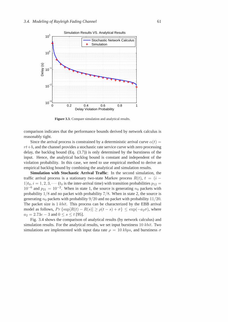
3.4. Modeling of Rayleigh Fading Channel 61
0 0.2 0.4 0.6 0.8 110
−3
10−2
10−1
100
101
Simulation Results VS. Analytical Results
Delay Violation Probability
Del
ay (
s)
Stochastic Network CalculusSimulation
Figure 3.3. Compare simulation and analytical results.
comparison indicates that the performance bounds derived by network calculus isreasonably tight.
Since the arrival process is constrained by a deterministic arrival curveα(t) =rt+b, and the channel provides a stochastic rate service curve with zero processingdelay, the backlog bound (Eq. (3.7)) is only determined by the burstiness of theinput. Hence, the analytical backlog bound is constant and independentof theviolation probability. In this case, we need to use empirical method to derive anempirical backlog bound by combining the analytical and simulation results.
Simulation with Stochastic Arrival Traffic : In the second simulation, thetraffic arrival process is a stationary two-state Markov processR(t), t = (i −1)t0, i = 1, 2, 3, · · · (t0 is the inter-arrival time) with transition probabilitiesp12 =10−6 andp21 = 10−2. When in state 1, the source is generatingn0 packets withprobability1/8 and no packet with probability7/8. When in state 2, the source isgeneratingn0 packets with probability9/20 and no packet with probability11/20.The packet size is1 kbit. This process can be characterized by the EBB arrivalmodel as follows,Pr {sup[R(t)−R(s)] ≥ ρ(t− s) + σ} ≤ exp(−a2σ), wherea2 = 2.73e− 3 and0 ≤ s ≤ t [95].
Fig. 3.4 shows the comparison of analytical results (by network calculus) andsimulation results. For the analytical results, we set input burstiness10 kbit. Twosimulations are implemented with input data rateρ = 10 kbps, and burstinessσ

62 Chapter 3. Channel Modeling and Bandwidth Estimation
0 0.2 0.4 0.6 0.8 110
−1
100
101
102
Simulation Results VS. Analytical Results
Violation Probability
Del
ay (
s)
Stochastic Network CalculusSimulation: σ = 10 kbSimulation: σ = 5 kb
Figure 3.4. Compare simulation results with analytical results: Markov arrivals.
equals to5 kbit and10 kbit, respectively. The input burstiness denotes the maxi-mum number of packets that the source generates at a time. For example,σ = 5corresponds ton0 = 5 andt0 = 0.5 s, andσ = 10 corresponds ton0 = 10 andt0 = 1 s. From the comparison, we can see that both simulation results are withinthe bounds of analytical results, which validate the correctness of the analyticalmethod. Furthermore, with the same setting of input burstiness, i.e.,σ = 10 kbit,the simulation and analysis results are very close to each other. The maximum,average, and minimum differences between them are8.25%, 10.5% and15.8%,respectively. The comparison indicates that the tightness of delay bound derivedby network calculus is acceptable.
Numerical Results
In the first experiment, the performance bounds are studied under the case ofa periodic traffic source sending packets over the Rayleigh fading channel. Thetraffic input process is modeled an affine arrival curve [11], which isdefined asα(t) = rt+ b, whereb andr represent the burst tolerance (inbits) and the averagedata rate (inbit/s), respectively. In this experiment, we setb = 1 kbit andr =10 kbps.

3.4. Modeling of Rayleigh Fading Channel 63
24
68
10x 10
4
−10
0
10
20
0
0.2
0.4
0.6
0.8
1
Tx Data Rate (bit/s)SNR (dB)
Vio
latio
n P
roba
bilit
y
Figure 3.5. Delay bound under different SNR and transmission data rates.
24
68
10x 10
4
−10
0
10
200
0.02
0.04
0.06
0.08
0.1
Tx Data Rate (bit/s)SNR (dB)
Del
ay B
ound
(s)
Figure 3.6. Violation probability of the delay and backlog bounds.
If R ≥ r 2, the delay bound can be calculated byh(α, β) = b/R, and the
2If R < r, both the delay and backlog would increase with time. It is impossible and meaninglessto find the finite delay and backlog bounds. Therefore, we consider the case thatR ≥ r.

64 Chapter 3. Channel Modeling and Bandwidth Estimation
backlog bound isα⊘ β(0) = b. Fig. 3.5 shows the values of delay bound varyingwith R ∈ [10 kbps, 100 kbps] andSNR ∈ [−10 dB, 20 dB]. The delay bounddis determined by the input burstinessb and the transmission data rateR. From Fig.3.5, we can see that with a fixedb, the delay bound increases as transmission rateincreases, and it is independent of the SNR. The backlog bound is only determinedby the burstiness of the input traffic. However, the corresponding violation prob-abilities of these two bounds are impacted both by the transmission data rate andSNR (as shown in Fig. 3.6). The violation probability increases as transmissiondata rate increases and/or SNR decreases. There is a trade-off between the delaybound and its violation probability. If we want to reduce the transmission delay,a high transmission rate should be chosen. But high transmission rate bringshighviolation probability.
The analysis method not only can be used to derive performance boundsandtheir corresponding violation probabilities, but also can provide guidelinesfor de-signing modulation and coding schemes, i.e., the designer can choose appropriatetransmission strategies according to performance requirements. For example, if theperformance requirement is given as:d < 0.02 ( as shown by the plane in Fig. 3.5)with violation probability less than10% (as shown by the plane in Fig. 3.6), we canget the following system configurations:R > 50 kbps andSNR > 14dB, whichare the values constraining delay and violation probability within the threshold.Hence, the designer can choose corresponding transmission strategy (transmissionpower, modulation and coding schemes) according toR andSNR.
Numerical Results with Stochastic Arrival Traffic : In the following experi-ments, we study the performance bounds under the case of a random traffic sourcesending packets over the Rayleigh fading channel. The traffic input process is mod-eled by the EBB arrival curve (Eq. (3.13)). The values of parametersare:a1 = 1,a2 = 1e − 3, andρ = 10 kbps. Similar to the previous experiment, it is assumedρ ≤ R.
In this experiment, the transmission data rate is set toR = 30 kbps, and thevalues of input burstiness (σ) and SNR are changed. Both the delay (d = σ/R)and backlog (B = σ) bounds are linearly increasing with input burstiness. Theircorresponding violation probabilities are illustrated in Fig. 3.7, where we canseethat the violation probabilities decrease asSNR and/orσ increase. Hence, thereare trade-offs between performance bounds and their violation probabilities. Highσ would cause low violation probability, but bring high delay and backlog. There-fore, appropriate values ofσ andSNR should be chosen according to the perfor-mance requirements.
In this experiment, we fix theSNR = 10 dB and change the values of input

3.4. Modeling of Rayleigh Fading Channel 65
−100
1020
20004000
60008000
10000
0
0.2
0.4
0.6
0.8
1
SNR (dB)
Burstiness Constraint on Input (bits)
Vio
latio
n P
roba
bilit
y
Figure 3.7. Violation probability of the delay and backlog bounds.
24
68
10x 10
4
20004000
60008000
10000
0
0.2
0.4
0.6
0.8
1
Tx Data Rate (bit/s)
Burstiness Constrainton Input (bits)
Del
ay B
ound
(s)
Figure 3.8. The delay bound.
burstiness (σ) and transmission data rateR. Similarly, the backlog bound is onlydetermined byσ. The delay bound is shown in Fig. 3.8. The violation probabilitiesof these two bounds are illustrated in Fig. 3.9.
From Fig. 3.8, we can see that the delay bound increases as input burstiness

66 Chapter 3. Channel Modeling and Bandwidth Estimation
24
68
10
x 104
20004000
60008000
10000
0
0.2
0.4
0.6
0.8
1
Tx Data Rate (bit/s)
Burstiness Constraint on Input (bits)
Vio
latio
n P
roba
bilit
y
Figure 3.9. Violation probability of the delay and backlog bounds.
increases, and it decreases as transmission data rate increases. While the viola-tion probability of the bounds has an opposite behavior, i.e., it decreases as theinput burstiness increases and it increases as the transmission data rate increases.Moreover, from these performance results we can derive the system configurationswhich can meet the requirements. For example, if the performance requirementsare defined as:d < 0.15 s, B < 5 kbit with violation probability less than10%,then we should select the values ofSNR andσ below the planes in Fig. 3.8 andFig. 3.9.
3.5 Bandwidth Estimation through Backlog Measurement
3.5.1 Preliminaries
Based on the min-plus algebra and max-plus algebra, network calculus cantransform complex network systems into analytically tractable systems [11, 46].LetR(t), S(t), andR∗(t) denote the arrival process, service process, and departureprocess of a system, respectively. Their relations can be defined as follows,
R∗(t) = R⊗ S(t) = inf0≤τ≤t
{R(τ) + S(t− τ)} (3.17)
where⊗ denotes the min-plus convolution. In the min-plus algebra, the service ca-pability of a system is expressed in terms of service curves. For wireless networks,

3.5. Bandwidth Estimation through Backlog Measurement 67
it is very difficult, if not impossible, to find deterministic service guarantees due tothe stochastic nature of wireless channels. A popular way to model the stochasticservice process is usingstatistical service curve[14], which provides probabilisticabstraction of the service guarantees.
A non-decreasing functionS(t) is a statistical service curve of the system, if
Pr{R∗(t) ≥ R⊗ S(t)
}> 1− ξ (3.18)
whereξ denotes the violation probability (0 ≤ ξ ≤ 1). The statistical service curveprovides a probabilistic abstraction of the service at a system, which is expressedby a deterministic service curve (S(t)) and a corresponding violation function.
The objective of our bandwidth estimation framework is to model the servicecapability of wireless channels. Since it is very difficult to derive the exact serviceprocessS(t) due to the randomness of the channels, we try to derive its corre-sponding statistical service curveS(t).
Lemma 3.3: For a system with service processS(t), any functionS(t) thatsatisfies,
Pr{S(t) ≥ S(t)
}> 1− ξ (3.19)
for 0 ≤ t ≤ T , is a statistical service curve of the system, whereT is a limit onthe maximal time scale on which the service curve relates service guarantees toarrivals [14]. The detailed proof of this lemma is presented in [14] [64].
The bandwidth utilization (real service) of a wireless channel is determinedbyits channel characteristics, behaviors of the sender and the receiver. It can be re-flected by the amount of backlogged traffic at the sender. Therefore,the channelbandwidth estimation can be implemented by measuring the backlog at the senderthrough sending probe packets. We adopt therate scanningprobe scheme pro-posed in [57], where the packets are organized in packet trains. The probe packettrains are injected and the backlog bounds are measured. Based on the Legendretransform [57], the statistical service curve and bandwidth are derived through themeasured backlog bounds.
According to the traffic pattern of probe packets, the arrival processat thesender can be expressed byR(t) = rt, wherer is the transmission rate of theprobe train. Given the arrival and departure functionsR(t) = rt andR∗(t), thebacklog bound is derived by [46],
B(r) = supt{R(t)−R∗(t)} = sup
t{rt−R∗(t)} (3.20)

68 Chapter 3. Channel Modeling and Bandwidth Estimation
Due to the stochastic behavior of the wireless channel, the backlog bound isalsostochastic. We can model the stochastic backlog bound by a statistical backlogbound, which is formally defined by the following equation,
Pr {B(r) ≤ Bǫ(r)} > 1− ǫ (3.21)
whereBǫ(r) denotes the statistical backlog bound with a violation probabilityǫwhen the probing rate isr. The following proposition formalizes the bandwidthestimation method.
Proposition 1: Consider a system with probing packet trains constrained bythe arrival curveR(t) = rt. Based on the measurement of the statistical backlogboundBǫ(r), the statistical service curve of the system can be derived by3,
S(t) = supr
{rt−Bǫ(r)} (3.22)
where the violation probability of the statistical service curve is calculated byξ =min(
∑r ǫ, 1).
Proof: According to Eq. (3.20), the backlog bound of a system can be cal-culated byB(r) = supt {rt−R∗(t)}. Based on Eq. (3.17) and the Legendretransform [57] [64], the relations of backlog and service curve can be expressed as,
B(r) = supt
{rt− S(t)} ⇒ S(t) = supr
{rt−B(r)} (3.23)
From Eq. (3.21), we have
Pr {B(r) ≤ Bǫ(r)} > 1− ǫ
⇒Pr {rt−B(r) ≥ rt−Bǫ(r)} > 1− ǫ(3.24)
By the application of union bound (Eq. (3.17) in [46]), it follows that,
Pr
{S(t) ≥ sup
r{rt−Bǫ(r)}
}> 1−
∑
r
ǫ (3.25)
If we define S(t) = supr {rt−Bǫ(r)}, it completes the proof.S(t) is astatistical service curve of the system with the violation probability calculated byξ =
∑r ǫ. Since the probability is non-negative, we setξ = min(
∑r ǫ, 1).
Proposition 1 relates the statistical backlog bound with the statistical servicecurve based on the Legendre transform. Service curve for random wireless chan-nels can be estimated by using probe packet trains transmitted at different rates.Since the service curve is expressed as the integration of instant servicerate overtime, the bandwidth (service rate) is equal to the slope of statistical service curve.
3We have independently given and proved the proposition. Later we found that this propositionmatches an online publication [63].

3.5. Bandwidth Estimation through Backlog Measurement 69
3.5.2 Backlog-Based Bandwidth Estimation
After establishing the theoretic foundation of the bandwidth estimation methodin Section 3.5.1, a detailed estimation procedure is given as follows.
Let a probe packet train be composed ofN0 packets with lengthl. The trans-mission time interval between two adjacent packets isT0. The transmission rate(denoted byr) of a probe train is calculated byr = N0 · l/[T0(N0 − 1)]. Probepacket trains with the same rate are repeatedly injected into the system and thebacklogs are measured according to pre-defined sampling rates. Subsequent probepacket trains are injected with increasing rates until the system is saturated.Thebandwidth estimation procedure can be divided into three iterative steps. Fig. 3.10shows the flow chart of the estimation algorithm.
Start
Inject a probe
packet train
Values are
stationary ?
NO
YES
Calculate the max
backlog value;
Set J=J+1, M0= J.
Initialize M, M0, r;Set I=0,J=0
Obtain a set of
backlog values;
Set I = I+1
I<= M
Discard this set of
values
M0/M >
NO
YES
NO
End
Increase r;Set I=0, J=0
Calculate
B (r)
YES
Figure 3.10.Procedure of the bandwidth estimation method
• Inject packet train and obtain stationary backlog

70 Chapter 3. Channel Modeling and Bandwidth Estimation
From injecting a packet train with probe rater, we can obtain a set of backlogvalues at different time points from the measurements. If the values are stationary(i.e. steady-state), we keep them and calculate the max valueBmax(r). If thevalues are not stationary, they are discarded. The stationarity of the backlog seriescan be detected by using the square root test from Elliot, Rothenberg andStock(RES) [64] [32]. The ERS test is based on an autoregressive moving average modelwhich returns a single value called ERS statistic. If the ERS statistic falls below athreshold value, the data series is considered as stationary.
• Calculate statistical backlog boundIn the experiment, each packet train (with rater) is sent forM times andM0
(M0 <= M ) steady-state values of maximum backlogBmax(r) can be obtained.If M0/M > θ 4, it means that most of the measurements of backlog values arestationary. Then, the probe rate is increased and a new probe packet train is sent.Otherwise, it indicates that the probe rate is too high, leading to system saturation.In this case, the probe rate increase is stopped and the program ends.
In order to obtain the statistical backlog bound from a large amount of mea-surements, we apply the statistical method calledquantile(Chapter 2 in [12]). Ap%-quantile leavesp% of the measurement values below and(100 − p)% abovewith certain confidence levels. It is defined as follows. Assume there aren datapointsx1, ..., xn from the measurements. Sort the points in an increasing orderand obtainx(1) ≤ ... ≤ x(n). Thep%-quantile is defined as(xk′ + xk′′)/2 withk′ = ⌊p(n− 1)/100 + 1⌋ andk′′ = ⌈p(n− 1)/100 + 1⌉. ⌊u⌋ is the largest inte-ger not bigger thanu and⌈u⌉ is the smallest integer not less thanu. The quantilereveals information about the dispersion of the observations of random variables.It consists of an upper bound and a lower bound. Based on the quantile principle,theseM0 measurements of backlog bound are quantified and we can get the upperand lower bounds ofp%-quantile of the backlog bound (denoted byBǫ(r)) withcertain confidence levels (the typical value of confidence level is0.95).
• Bandwidth estimationEach probe rater reveals one pointBǫ(r) of the service curve in the Leg-
endre domain, which composes a piecewise linear segment of the service curveS(t) = rt − Bǫ(r). The probe rate of packet train is increased and the probepacket train is sent repeatedly until the proportion of stationary measuredbacklogvalues is below the threshold (i.e.M0/M ≤ θ). According to Proposition 1, wecan re-build the estimated statistical service curve, which is composed of piecewiselinear segments. Since the service curve is expressed as the integration ofinstant
4θ denotes the threshold of the proportion of valid measurements that can produce stationarybacklog values.
3.5. Bandwidth Estimation through Backlog Measurement 71
service rate over time, the bandwidth can be derived by calculating the slopeof thestatistical service curve.
3.5.3 Experimental Results
Experiment Purpose and Setup
Simulations are conducted to validate the estimation method. The sender trans-mits probe packet trains to the receiver through a time-variant Rayleigh fadingchannel. Consider a slow fading channel so that the capacity does not changeduring the transmission of one packet. A packet train contains1000 packets, andthe arrival interval between two adjacent packets is9 ms. The length of a packetchanges from100 bits to 3000 bits with an increment of100 bits in each step.Hence, the corresponding probe data rate varies from11 kbps to 330 kbps with anincrement of11 kbps. For each probe rate, the simulation runs1000 times. Thevalues of backlog are recorded every millisecond until the last packet has been sent.Since the results are not sensitive to the value of thresholdθ, θ is set to0.8 as anexample.
0 1000 2000 3000 4000 5000 6000 7000 8000 90000
20
40
60
80
100
120
140
160
180
200
220Service rate of Rayleigh channel
Time (ms)
Rat
e (k
bps)
Stochastic service rate95%−quantile(low)95%−quantile(upp)
Figure 3.11.Service rate of Rayleigh channel
The channel capacity of the Rayleigh channel is given byC = BW · log2[1 +S/(BW · δ0)], whereBW denotes the channel bandwidth,δ0 is the noise power,

72 Chapter 3. Channel Modeling and Bandwidth Estimation
andS represents the received signal power. We setBW = 30 kHz, δ0 = −55dBm (3.3 × 10⁻⁹ W ), andS is an exponential distributed random variable witha mean of2 × 10−3. Fig. 3.11 illustrates a realization of the service rate whichis defined as the capacity of the channel. The95%-quantile of the service rate isobtained by using the method described in Section 3.5.2.
Estimation Results
In each simulation run, a backlog bound is recorded if the set of backlog resultsare stationary (Section 3.5.2). These backlog bounds are quantified to obtain thestatistical backlog bound. Fig. 3.12 shows the99%-quantile of the upper and lowerbounds of maximum backlog with confidence level of95%.
Figure 3.12.Maximum backlog for different probing rates.
Both the statistical service curves of the reference and estimation are expressedby deterministic service curves and corresponding violation probabilities. Fig. 3.13shows the comparison ofreference service curve(Ref SC) and theestimated ser-vice curve(Est SC). The confidence level of them are95%. The reference servicecurve is described by a rate service curve with rate in the range[173, 185] kbpsand the violation probability of5% (as shown by the solid and dashed lines). In thesimulation, the estimated service curve is contributed by piecewise linear segmentswith 99%-quantile backlog bounds from5 different probe rates. So the violation

3.5. Bandwidth Estimation through Backlog Measurement 73
probability of the estimated service curve is5% (Eq. (3.25)). The estimated ser-vice curve is divided into two regions: starvation region and stable region.In thestarvation region, the service capability of the channel is higher than the input traf-fic rate. So the estimated bandwidth is smaller than the actual service rate. In thestable region, the estimated bandwidth is178 kbps, which is within the range ofthe reference service rate. The results in the stable region show that ourmethodcan accurately estimate the bandwidth.
0 1000 2000 3000 4000 5000 6000 7000 8000 90000
0.2
0.4
0.6
0.8
1
1.2
1.4
1.6
1.8
2x 10
6 Estimated SC vs. Reference SC
Time (ms)
Dat
a (b
its)
Ref SC (upp)Ref SC (low)Est SC (upp)Est SC (low)Est trials
Rate =173
Rate=185
Rate=178
Figure 3.13. Comparison of reference service curve and estimated service curve: insimulation trials, the probe packet trains are sent with various rates and thebacklogbounds are measured. The thin dashed blue lines represent the resultsof bandwidthestimation from all the trials.
In Fig. 3.14, the estimated bandwidth is compared with the reference servicerate (i.e. bandwidth) under different channel parameters. Since the difference be-tween the upper and lower bounds of the estimated bandwidth is very small, weonly show the mean value of the estimated bandwidth in the figure. From Fig.3.14, we can see that the estimated bandwidths are within the range of the upperand the lower bounds of the reference bandwidth for the second and fourth bargroups. When the channel bandwidth is20 kHz and the mean of the received sig-nal power is0.001, the estimated bandwidth is5% bigger than that of the upperreference bandwidth. For the third bar group, the estimated bandwidth is8% larger

74 Chapter 3. Channel Modeling and Bandwidth Estimation
than the upper reference bandwidth. The deviation is due to imprecise sampling ofbacklog measurement.
0
50
100
150
200
250
300
350
400Compare estimated bandwidth and reference bandwidth
Ban
dwid
th (
kbps
)
Ref bandwidth (low)Ref bandwidth (upp)Est bandwidth
BW=30kHzmean=0.002
BW=40kHzmean=0.002
BW=50kHzmean=0.003
BW=20kHzmean=0.001
Figure 3.14.Comparison of reference service curve and estimated service curvewithvarious channel parameters: 1) channel bandwidth; 2) mean of the received signalpower (in Watt).
We design the following experiment to study the impact of inter-packet intervaland packet size. In each simulation, the packet length is fixed, and we change theprobe data rate by varying the inter-packet interval from2ms to 20ms with an in-crement of1ms. The bandwidth isBW = 40 kHz, and the mean is0.002. Otherparameters remain the same. We run15 simulations with packet lengths increasingfrom 600 bits to 2000 bits. Fig. 3.15 illustrates the comparison of estimated band-width and reference bandwidth. As we can see, most of the estimated bandwidthare within the lower and upper bounds of the reference bandwidth. Only afew areslightly deviated from the reference because of sampling effect. In summary, fromFig. 3.14 and Fig. 3.15, we can see that the accuracy of the method is satisfactoryunder different channel characteristics, packet sizes, and inter-packet intervals.
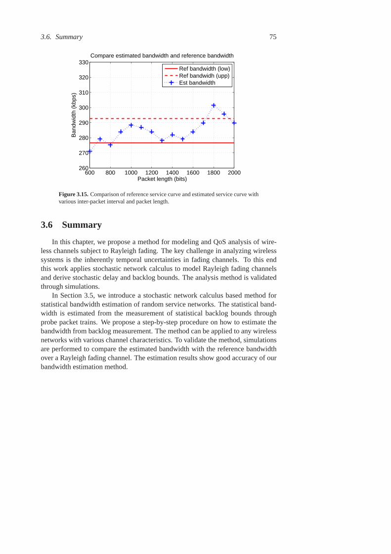
3.6. Summary 75
600 800 1000 1200 1400 1600 1800 2000260
270
280
290
300
310
320
330
Packet length (bits)
Ban
dwid
th (
kbps
)
Compare estimated bandwidth and reference bandwidth
Ref bandwidth (low)Ref bandwidh (upp)Est bandwidth
Figure 3.15.Comparison of reference service curve and estimated service curvewithvarious inter-packet interval and packet length.
3.6 Summary
In this chapter, we propose a method for modeling and QoS analysis of wire-less channels subject to Rayleigh fading. The key challenge in analyzing wirelesssystems is the inherently temporal uncertainties in fading channels. To this endthis work applies stochastic network calculus to model Rayleigh fading channelsand derive stochastic delay and backlog bounds. The analysis method is validatedthrough simulations.
In Section 3.5, we introduce a stochastic network calculus based method forstatistical bandwidth estimation of random service networks. The statistical band-width is estimated from the measurement of statistical backlog bounds throughprobe packet trains. We propose a step-by-step procedure on how toestimate thebandwidth from backlog measurement. The method can be applied to any wirelessnetworks with various channel characteristics. To validate the method, simulationsare performed to compare the estimated bandwidth with the reference bandwidthover a Rayleigh fading channel. The estimation results show good accuracy of ourbandwidth estimation method.

76

Chapter 4
Coverage and Deployment
This chapter presents our research on coverage analysis and deployment tech-niques in wireless sensor networks. The work in this chapter is mainly basedon[88, 91, 92].
4.1 Introduction
One fundamental application of WSNs is event detection in a Field of Inter-est (FoI), where a set of sensors are deployed to monitor any ongoingevents. Forexample, sensor networks can be deployed to detect the occurrences of fires, earth-quakes, volcanic eruptions, and motions of wild animals [3, 27, 102]. To satisfy acertain level of detection quality in such applications, it is desirable that events inthe region can be detected by a required number of sensors. Hence, animportantproblem is how to deploy sensor nodes for achieving certain coverage require-ments.
Coverage analysis in WSNs has attracted plenty of research interests [59, 100,52, 6, 8, 115, 108]. One of the most popular metrics to quantify the coverage per-formance isk-coverage [43, 113]. An FoI is said to bek-covered if every point in itis covered by at leastk sensors. The coverage problem can be classified in differentways depending on the way of sensor deployment and the features of applications.Based on the characteristics of applications, thek-coverage problem can be cat-egorized intoarea coverageandevent coverage, where the former requires eachlocation within the sensing field must be covered by at leastk sensors. While theobjective of event coverage analysis is to study how well the events in the sensingfield are detected. Fig. 4.1 shows an example of area coverage and event coverage(As an example, the FoI in this figure is a rectangle. However, in our analysis the
77

78 Chapter 4. Coverage and Deployment
FoI can be irregular). In the left figure, the purpose is to ensure the whole area ofthe FoI is covered by sensors. In the right figure, the purpose is to ensure the eventsin the FoI are covered by sensors.
Field of Interest
Event
Sensor and its
sensing region
Figure 4.1. Left: area coverage; right: event coverage
In many applications, the tasks of sensor networks are monitoring or detectingevents, such as the behaviors of animals in a forest [93]. For those scenarios,covering of locations does not mean covering of events. For example, in aWSNapplication, we need to deploy video sensors in a forest to monitor the behaviors ofwild animals, and a sensor can not monitor two animals simultaneously. Assumefive video sensors can cover the whole area of the forest from the analysis of areacoverage. However, if more than five animals enter into the monitoring region,five sensors are not able to track the activities of all the animals. To study theperformance of coverage in those cases, we need event coverage analysis method.However, there is very few research on event coverage analysis considering botharea coverage analysis and event occurrence.
In this chapter, a probabilistic event coverage analysis method is proposed forevaluating the coverage performance of heterogeneous sensor networks with ran-domly deployed sensors and stochastic event occurrences. Different from tradi-tional area coverage analysis, the event coverage is to quantify the probability thatevents can be covered by sensors, given the density of events and thedensity of sen-sor deployment. We provide formulas to calculate event coverage probability underdifferent settings of sensor and event densities with the considerations of boundaryconditions. Moreover, the event coverage analysis is extended to heterogeneoussensor networks. In this chapter, we define heterogeneous sensor network as thenetwork where the sensor distribution in the FoI is heterogeneous. As shown in Fig.4.2, in the homogeneous network, the sensor density in the whole FoI is uniform.

4.2. Related Work 79
In the heterogeneous network, the FoI is logically divided into sub-FoIs accordingto the event density. In different sub-FoIs, the sensors are deployed with differ-ent densities. The probability of event coverage in heterogeneous sensor networksis derived. The analytical results show how the probabilities of event coveragechange with the sensor and event densities. Moreover, the results also indicate thatfor sensor networks with irregular event occurrence, heterogeneous sensor deploy-ment can achieve better coverage performance than homogeneous deployment. Inaddition, the comparisons of simulation and analytic results validate our proposedevent coverage analysis method. This method can provide guidelines in determin-ing how many sensors are required to guarantee a certain level of coverage forgiven users’ requirements and characteristics of applications.
Figure 4.2. Left: heterogeneous sensor networks; right: homogeneous sensornet-works
4.2 Related Work
In recent years, a host of research activities have been performedon coverageanalysis in sensor networks regarding to different objectives and metrics [38, 52,59, 100, 101, 7]. These work can be divided into two classes of coverage analysis:area coverage and event coverage [94].
Liu and Towsley in [59] defined three coverage measures to characterize areacoverage, node coverage and detectability in large-scale sensor networks. Theystudied the coverage problem from a theoretical perspective and explored the fun-damental coverage limits. In [52], the authors studied the problem of stochasticcoverage in heterogeneous sensor networks. By mapping the coverage problem tothe set intersection problem, they provided formulas fork-coverage in the caseswhere sensors’ sensing regions can have any arbitrary shapes. Gupat et al. [38]

80 Chapter 4. Coverage and Deployment
investigated the problem of choosing the minimum number of sensors from a setof sensors that are uniformly deployed such that the FoI is covered. In[100],the authors have studied the asymptotic node density requirement for achieving k-coverage in uniformly random deployment and Poisson process deployment. Fur-thermore, Zhang and Hou [112] proposed a different method to derivethe sufficientand necessary node densities for maintaining k-coverage for a given sensor networkunder both random and deterministic deployment strategies.
Clouqueuret al. [23] formulated the target detection problem as an unautho-rized traversal problem and proposed deployment strategies which canachieve therequired target detection probability and minimize the network cost. In the de-ployment strategy, only part of the sensors are randomly deployed if those sensorscan ensure the coverage performance. In [103], the authors considered a hybridsensor network consisting of static and mobile sensor. Static sensors are fixedto detect events and mobile sensors move closer to such events when they are de-tected. In [53], the authors mapped the target detection problem in sensornetworksto a line-set intersection problem. Based on that, the probability of detecting tar-gets is analytically evaluated for both deterministic and stochastic deployment. In[94], Snyderet. al proposed an efficient sensor movement strategy to detect thedynamic events in sparse mobile sensor networks. The locations and durations ofevents in the network are dynamic. Baiet al. [7] studied the problem of achievingoptimal multiple-coverage with minimum number of sensor nodes. Their proposedresults are helpful in constructing two-coverage deployment patterns withcertainoptimization.
4.3 Probabilistic Event Coverage
In this section, we derive the probability of event coverage when the sensorsand events are distributed according to the spatial Poisson process. In order to dothat, it firstly needs to derive the probability of area coverage.
4.3.1 System Model
Spatial Poisson Process
A spatial point process is a model for a random pattern of points ind-dimension(d = 2 in this paper) space. It can be used as statistical models in the analysis ofobserved patterns of locations of objects, such as animals in forests and sensors ina building. One of the most popular spatial point processes is thespatial Poissonprocess[5], which is formally defined as follows.

4.3. Probabilistic Event Coverage 81
Definition 4.1 Spatial Poisson Process:For an FoIA0 with areaF0, the spatialPoisson process, with a uniform intensityλ > 0, is a point process inR2 such that
1) The number of eventsM(A0) in the FoIA0 has a Poisson distribution withmeanλF0;
2) If A10, · · · , Am
0 are disjoint regions inA0, thenM(A10), · · · , M(Am
0 ) areindependent.
The intensityλ is defined as the expected number of targets per unit area.
Network Model
Consider a two-dimensionField of Interest(FoI) A ∈ R2. Sensors are placedinside the FoI randomly according to a spatial Poisson process of intensityλ > 0.Thus for any regionAi ⊆ A, the number of sensors inAi is given by a Poissonvariable of meanλ |A ∩Ai|, where|A ∩Ai| is the area of the regionAi. Assumeall sensors have homogeneous sensing regions which can be irregularshapes. Theevent occurrence in the FoI is also modeled by the spatial Poisson point process,which is a random collection of points representing the location of events. A targetevent is said to be covered if and only its distance to the nearest sensor is equal toor less than the sensing range. Equivalently, given a target, the probability it is notcovered by any sensors is equal to the probability that it is not within the range ofany sensor or enough number of sensors. In event-driven sensornetworks, the pur-pose is to detect event occurrences. Sensors start to work and collect informationonly when there are events within their sensing ranges.
In some applications of sensor networks, the probability of event occurrence indifferent regions of the FoI are different. In order to provide good coverage in thesenetworks, we adopt the heterogeneous sensor deployment method. Namely, thedensity of sensor deployment in different regions of the FoI are different dependingon the event occurrence probability. Details are given in Section 4.3.5.
4.3.2 Area Coverage
Basically, the probabilistic area coverage can be formulated as follows: A num-ber of sensors are randomly deployed in an FoI. The areas and perimeters of theFoI and the sensing region of each sensor are given. We need to calculate the prob-ability that a random point in the FoI is monitored by at leastk sensors, namely, itis k-covered. In [52], the authors mapped this stochastic coverage problem into aset intersection problem and proposed an analytic method to derive the probabilityof k-coverage based on integrate geometry. The detailed descriptions are definedas follows:

82 Chapter 4. Coverage and Deployment
Lemma 4.1Let A0 be an FoI with areaF0 and perimeterL0 on a plane.N(N ≥ 1) sensors are uniformly randomly deployed in the FoIA0. The area andperimeter of the sensing region of each sensor are denoted byFs andLs, respec-tively. Let P1(N, k) andP2(N, k) represent the probability that a randomly se-lected point inA0 is covered by exact and at leastk sensors, respectively. For1 ≤ k ≤ N , we have
P1(N, k) =
(Nk
)(2πFs)
k(2πF0 + L0Ls)N−k
[2π(F0 + Fs) + L0Ls]N, (4.1)
P2(N, k) = 1−k−1∑
i=0
P1(N, i) (4.2)
The boundary condition isP1(N, 0) = P2(N, 0) = 1. For simplicity, we as-sume the sensing regions of all sensors are homogeneous. However, itis proposedin [52], the derivations can be easily extended to the cases with heterogeneoussensing regions as long as the area and perimeter of each sensor are given.
In our network model, sensors are deployed in the sensing field according to aspatial Poisson process. The probability of k-coverage can be derived as follows.
Lemma 4.2Let A0 be an FoI with areaF0 and perimeterL0 on a plane. Sen-sors are deployed in the FoIA0 according to a spatial Poisson process with intensityλ. The area and perimeter of the sensing region of each sensor are denoted byFs
andLs, respectively. LetPex(λ, k) andPle(λ, k) denote the probability that a ran-domly selected point inA0 is covered by exact and at leastk sensors, respectively.We haveP ex
c (λ, 0) = P lec (λ, 0) = 1, and fork ≥ 1,
Pex(λ, k) =∞∑
j=k
(jk
)e−λF0(λF0)
j(2πFs)k(2πF0 + L0Ls)
j−k
j!× [2π(F0 + Fs) + L0Ls]j(4.3)
Ple(λ, k) = 1−k−1∑
i=0
Pex(λ, i) (4.4)
Proof: If the sensors are deployed according to a spatial Poisson process withintensityλ, the probability that there arej sensors in the FoIA0 is given by,
P {N(A0) = j} =(λF0)
j
j!e−λF0 (4.5)

4.3. Probabilistic Event Coverage 83
Given there arej sensors, the probability of exact k-coverage is given by Eq.(4.1) . By summing up all the possibilities, we can get
Pex(λ, k)
=∞∑
j=k
P {N(A0) = j}P1(j, k)
=∞∑
j=k
(jk
)e−λF0(λF0)
j(2πFs)k(2πF0 + L0Ls)
j−k
j!× [2π(F0 + Fs) + L0Ls]j
(4.6)
Consequently, the probability of at least k-coveragePle(λ, k) equals to oneminus the sum of the probabilities of less than exact k-coverage.
4.3.3 Event Coverage
The objective of this work is to study the probabilistic event coverage problem,which is different from traditional area coverage problem in WSNs. Generally,the event coverage is to quantify how well the events in an FoI is detected bysensors. The probabilistic event coverage problem is described as: Given an FoI,events may happen in any points of the FoI, and multiple sensors are deployedin the FoI to detect the events. Both sensors and events are distributed accordingto the spatial Poisson process. We need to compute the probability that a randomevent can be detected by at leastk sensors. In this problem, the probability of eventcoverage depends on not only the intensity of events but also the intensity of sensordeployment. The event coverage is formally defined as follows:
Lemma 4.3In an FoIA0 with areaF0 and perimeterL0, sensors are deployedaccording to a spatial Poisson process with intensityλ. The area and perimeter ofthe sensing region of each sensor are denoted byFs andLs, respectively. Eventsmay happen inA0 and they are modeled by a spatial Poisson process with intensityγ. Let Pe−cov(k) denote the probability that every event is detected by at leastksensors. Then, we have
Pe−cov(k)
=∞∑
n=1
{P [M(A0) = n] [Ple(λ, k)]n}
=
{∞∑
n=1
(γF0)n
n!e−γF0 [1−
k−1∑
i=0
Pex(λ, i)]n
}(4.7)

84 Chapter 4. Coverage and Deployment
whereq0 denotes the probability that a given event is detected by less thanksensors. The value ofk depends on the requirements of applications. For example,k = 1 can meet the requirements of monitoring applications, while in tracking orpositioning applications,k might be2 or 3.
4.3.4 Boundary Analysis
For sensors deployed near the boundary of the FoI, part of the coverage regionsare outside the FoI. The coverage analysis should take this issue into account.
O
BCD
rs
(a)
(b)
Figure 4.3. Boundary analysis
Thenear boundary regionis defined as the the region with distancers to theboundary (Fig. 4.3-(a)), wherers denotes the maximum sensing distance of thesensors. As shown in Fig. 4.3, a sensors is located at pointO which is insidethe near boundary region of the FoI. Letz (0 < z < rs) denote the distancebetween the sensor and the boundary of the FoI (OC = z). From basic geometryknowledge, we know that the value of∠BOC equals toarccos(z/rs) .

4.3. Probabilistic Event Coverage 85
Therefore, the area of the shadow region (⌢ DBC) in Fig. 4.3-(b) is calculatedby,
Fshd = r2s arccosz
rs− z√r2s − z2 (4.8)
For the sensors located in the near boundary region, the ratio of the coverageregion inside the FoI is calculated by,
ηz = 1− r2s arccos(z/rs)− z√r2s − z2
πr2s(4.9)
For a randomly deployed sensor in the near boundary region, the probability itis located in a strip (dz) with distancez to the boundary is given by,
qz =(L0 − νz)dz
F0 − F′
0
(4.10)
whereF′
0 denotes the area of the FoI excluding the near boundary region,ν is aconstant depending on the shape of the FoI. If the FoI is a rectangle, thevalue ofνis 8. If the FoI is a circle, the value ofν is 2π. Hence, the mean coverage ratioη0is calculated by,
η0 =
∫ rs
0
L0 − νz
F0 − F′
0
[1−
r2s arccoszrs
− z√
r2s − z2
πr2s
]dz (4.11)
The detailed computation of Eq. (4.11) is described in the following.Eq. (4.11) can be re-organized as follows,
η0 =
∫ rs
0
L0 − νz
F0 − F′
0
dz
+
∫ rs
0
νr2sz arccoszrs
− L0r2s arccos
zrs
(F0 − F′
0)πr2s
dz
+
∫ rs
0
L0z√r2s − z2 − νz2
√r2s − z2
(F0 − F′
0)πr2s
dz
(4.12)
In the above equation,rs, F0, F′
0, L0, ν are non-integration variables. It is easyto compute the first part of Eq. (4.12) as follows,

86 Chapter 4. Coverage and Deployment
∫ rs
0
L0 − νz
F0 − F′
0
dz =2L0rs − νr2s2(F0 − F
′
0)(4.13)
According to the formula (306) in Chapter 7.4 of [28], we have
∫z arccos(az)dz =
z2
2arccos(az)
− 1
4a2
[arccos(az) + az
√1− a2z2
].
(4.14)
Based on the formula (304) in Chapter 7.4 of [28], we have∫
arccos(az)dz = z arccos(az)− 1
a
√1− a2z2. (4.15)
Consequently, the second part of Eq. (4.12) can be calculated based on theabove formulas.
Based on the formula (142) in Chapter 7.4 of [28], we can get,∫
z√c2 − a2z2dz = − 1
3a2(c2 − a2z2)3/2 (4.16)
Moreover, from the formula (143) in Chapter 7.4 of [28], we have
∫z2√
c2 − a2z2dz =− z
4a2(c2 − a2z2)
3
2 +c2z
8a2
√c2 − a2z2
+c4
8a3arcsin(az/c).
(4.17)
Therefore, the third part of Eq. (4.12) can be computed accordingly.Based on the above formulas,η0 can be calculated.So the amended event coverage probability with the consideration of boundary
condition can be derived by the following equation,
P′
e−cov(k) =F
′
0 + (F0 − F′
0)η0F0
· Pe−cov(k) (4.18)
4.3.5 Probabilistic Event Coverage in Heterogeneous Networks
In traditional coverage analysis methods, the heterogeneity of events areusu-ally not considered and the sensors are uniformly deployed with the same density

4.3. Probabilistic Event Coverage 87
over the FoI. In many sensor network applications, there are surveillance regionswith different types of events which require different numbers of sensors. More-over, in some scenarios, the probabilities of event occurrence in different regionsof the FoI are different. For example, the studies in [39] show that wildfireeventsoccur in clusters. For those applications with heterogeneous event distributions, itis better to deploy various numbers of sensors in different regions of theFoI. In thefollowing, we present the coverage analysis for sensor networks with homogeneousand heterogeneous sensor deployment.
Event Coverage in Heterogeneous Networks
In heterogeneous sensor networks, the probabilities of event occurrence in dif-ferent parts varies. Considering the heterogeneity of event occurrence, the sen-sor deployment is also heterogeneous. Let the FoI be divided into multiple sub-FoIs A1, A2, · · · , AH . The area, perimeter and event density of the regionAh
(1 ≤ h ≤ H) areFh, Lh, andγh, respectively. Letλh denote the sensor density inregionAh. If we consider the difference of event densities and deployment sensorswith different densities, the probability of event coverage in the regionAh can beexpressed as,
P covh (k) = Q ·
{∞∑
n=1
(γhFh)n
n!e−γhFh [1−
k−1∑
i=0
Pex(λh, i)]n
}(4.19)
wherePex(λh, i) is derived by Eq. (4.3).Q is the emendatory coefficient, which iscomputed by (refer to Section 4.3.4 for details),
Q =F
′
h + (Fh − F′
h)η0Fh
(4.20)
whereF′
h denotes the area ofAh excluding the near boundary region.In the homogeneous deployment case, the heterogeneity of event occurrence is
not considered and the sensors are deployed with the same density. The compu-tation of event coverage probability is similar except that the values ofλh in Eq.(4.19) are equal. It is a special case of heterogeneous deployment.
The overall event coverage probability of the network can be calculatedby thegeometric mean of the event coverage probabilities of all the regions,
P covnet (k) =
H
√√√√H∏
h=1
P covh (k) (4.21)
.

88 Chapter 4. Coverage and Deployment
The use of a geometric mean normalizes the ranges being averaged, so thatno range dominates the weighting, and a given percentage change in any of theproperties has the same effect on the geometric mean.
Overlap between Sub-FoIs
In Section 4.3.4, we derive the coverage analysis with the consideration ofboundary condition. However, the boundary analysis can not be directly appliedto the heterogeneous network since there are coverage overlaps between sub-FoIs.So we propose a method to analyze the overlap between sub-FoIs.
Figure 4.4. Coverage overlap
The two-sub-FoI case is taken as an example. As shown in Fig. 4.4, the FoIA0
is divided into two sub-FoIs,A1 andA2. LetF1, L1, andγ1 be the area, perimeterand event density ofA1, respectively. LetF2, L2, andγ2 be the area, perimeter andevent density ofA2, respectively. We consider the difference of event densities anddeploy sensors with different densities (denoted byλ1 andλ2) in A1 andA2.
According to the analysis in Section 4.3.4, for a sensor located in the nearboundary region ofA2 with distancez to the boundary, the ratio of its coverageregion overlapping withA1 can be calculated as,
ζz = 1− ηz =r2s arccos(z/rs)− z
√r2s − z2
πr2s(4.22)
For a randomly deployed sensor in the overlap region, the probability withwhich it is located in a strip (dz) with distancez to the boundary is given by,
q′
z =l1,2
F2 − F′
2
dz (4.23)

4.3. Probabilistic Event Coverage 89
whereF′
2 denotes the area of theA2 excluding the overlap region,l1,2 denotes thelength of the border ofA1 andA2. So the average coverage contribution from asensor inA2 is,
ζ1,2 =
∫ rs
0ζz
l1,2
F2 − F′
2
dz (4.24)
The computation ofζ1,2 can be found in the Appendix. Therefore, the eventcoverage probability is calculated by,
P cov1 (k) = P cov
1 (k) · F′
1λ1 + (F1 − F′
1)λ2ζ1,2F1λ1
(4.25)
whereP cov1 (k) is calculated according to Eq. (4.19). AndP cov
2 (k) can be similarlycomputed.
The overall event coverage probability of the whole FoIA0 is computed by,
P covnet (k) =
√P cov1 (k) · P cov
2 (k) (4.26)
We extend the analysis to a multi-sub-FoI network where a sub-FoI may havemultiple neighbors (i.e., adjacent sub-FoIs). LetAh denote the sub-FoI whichhas multiple neighbors (denoted byNBG(Ah)). For any of the neighborAi, theaverage coverage contribution from a sensor inAi to Ah is derived by ( accordingto Eq. (4.22), (4.23), (4.24)),
ζh,i =
∫ rs
0
r2s arccos(z/rs)− z√r2s − z2
πr2s· lh,i
Fh − F′
h
dz (4.27)
Consequently, the event coverage probability can be computed by,
P covh (k) = P cov
h (k)∏
Ai∈NBG(Ah)
Qh,i (4.28)
whereQh,i is derived by
Qh,i =F
′
hλh + (Fh − F′
h)λiζh,iFhλh
. (4.29)
After we compute the event coverage probability of each sub-FoI, the overallevent coverage probability of the FoI can be calculated according to Eq.(4.21).

90 Chapter 4. Coverage and Deployment
4.3.6 Experimental Results
To evaluate the coverage analysis method and to show the benefits and accuracyof the analysis method in heterogeneous sensor networks, numerical experimentsand simulations are conducted. The analytic and simulation results of the probabil-ity of event coverage are presented and compared under different settings of sensorand event densities.
Analytical Results
In the following experiments, the probability of event coverage in homoge-neous sensor networks is studied, namely, the sensor density and eventdensity indifferent locations of the FoI are the same. The FoI is a rectangle with lengthandwidth of 20 m and16 m, respectively. The sensing region of each sensor is a discwith radius3 m. So the area and perimeter of the sensing region are28.3 m2 and18.8 m2, respectively. The sensor densityλ denotes the average number of sensorin an unit area. Similarly, the event densityγ represents the average number ofevent in an unit area.
0 0.05 0.1 0.15 0.2 0.25 0.30
0.1
0.2
0.3
0.4
0.5
0.6
0.7
0.8
0.9
1Probability of event coverage
Sensor density
Pro
babi
lity
γ = 0.01γ = 0.02γ = 0.03γ = 0.05γ = 0.1
Figure 4.5. Probability of event coverage: 1-coverage
Fig. 4.5 and Fig. 4.6 illustrate the probabilities that every event in the FoI iscovered by at least one sensor and two sensors, respectively. As we can see in

4.3. Probabilistic Event Coverage 91
both figures, for the same event density, the probability of event coverage increaseswhen the sensor density increases. For the same sensor density, when the eventdensity increases, the probability of event coverage decreases. Given the eventdensity in an application and the requirements on event coverage, these analyticresults can be useful in determining the density of deployment and the total amountof sensors.
0 0.05 0.1 0.15 0.2 0.25 0.30
0.1
0.2
0.3
0.4
0.5
0.6
0.7
0.8
0.9
1Probability of event coverage
Sensor density
Pro
babi
lity
γ = 0.01γ = 0.02γ = 0.03γ = 0.05γ = 0.1
Figure 4.6. Probability of event coverage: 2-coverage
Fig. 4.7 shows the probabilities that every event in the FoI is at leastk-covered(k = 1, 2, 3, 4) when the event density changes. The sensor density is set to0.3.Similar with those in Fig. 4.5 and Fig. 4.6, we can find in this figure that theprobability of event coverage decreases when the event density increases. More-over, when the requirement onk-coverage is increased, the probability of eventcoverage significantly decreases. For example, when the event densityis 0.15, theprobability of 1-coverage and2-coverage are0.73 and0.16, respectively. Theseresults indicate that if the applications have higher coverage requirements,muchmore sensors need to be deployed. Consequently, the total deployment costs canbe significantly increased.
The following experiments are performed to show the benefits of heteroge-neous sensor networks. The coverage region of a sensor is the same as that in theprevious section. In the network settings, the FoI is divided into sub-FoIs, and theevent densities in different sub-FoIs are different. In homogeneousdeployment, the

92 Chapter 4. Coverage and Deployment
0 0.05 0.1 0.15 0.2 0.25 0.30
0.1
0.2
0.3
0.4
0.5
0.6
0.7
0.8
0.9
1Probability of event coverage
Event density
Pro
babi
lity
1−coverage2−coverage3−coverage4−coverage
Figure 4.7. Probability of event coverage with different values ofk (λ = 0.3)
sensor density in all sub-FoIs is the same. In heterogeneous deployment,the sensordensity in different sub-FoIs are different. In order to implement fair comparisons,the average sensor density in the FoI of these two deployment scenarios are set tobe equal. The overall event coverage probability of the network is calculated bythe geometric mean of the probabilities of all the sub-FoIs (Eq. (4.21)).
In Fig. 4.8, we compare the probabilities of1-coverage (1-cov) and2-coverage(2-cov) under homogeneous and heterogeneous deployment in a two-sub-FoI net-work. We also consider the overlapping between adjacent sub-FoIs in the hetero-geneous deployment. From this figure, we can see that the probabilities of both1-coverage and2-coverage of heterogeneous deployment are better than those ofhomogeneous deployment. It indicates that heterogeneous deployment can achievebetter coverage performance. Moreover, considering overlapping between adja-cent sub-FoIs can improve the event coverage probabilities since the sub-FoI canget coverage compensation contributed by the sensors in the near boundary regionof its adjacent sub-FoI. In addition, the simulation results show that the results ofoverlapping analysis are accurate.
In this experiment, the FoI is divided into sub-FoI 1 and sub-FoI 2. The eventdensity in sub-FoI 1 isγ1 = 0.03, and that (γ2) in sub-FoI 2 is changed from0.04 to0.16. In Fig. 4.9, we can see that the event coverage probabilities in heterogeneousdeployment are larger than those in homogeneous deployment. Moreover,when

4.3. Probabilistic Event Coverage 93
0 0.05 0.1 0.15 0.2 0.250
0.1
0.2
0.3
0.4
0.5
0.6
0.7
0.8
0.9Heterogeneous deployment VS homogeneous deployment
Sensor density
Pro
babi
lity
of e
vent
cov
erag
e
1−cov:hom1−cov:het1−cov:het,ovl1−cov: sim2−cover:hom2−cover:het2−cov:het,ovl2−cov:sim
Figure 4.8.Event coverage probabilities in two-sub-FoI networks ( event densityγ =0.03, 0.06). ’hom’ denotes homogeneous deployment; ’het’ denotes heterogeneoudeployment; ’ovl’ means ’overlapping’ between adjacent sub-FoIs are considered.
γ1 = 0.03, γ2 = 0.16, the gap of the event coverage probability between the twodeployment methods are bigger than those forγ1 = 0.03, γ2 = 0.12(0.08/0.04).The comparisons indicate that the coverage performance of heterogeneous deploy-ment is better than that of homogeneous deployment. And the improvement ismore significant when the heterogeneity of event density is more obvious.
The following experiment is conducted to check the scaling property of theheterogeneous deployment method. The FoI is divided into8 regions with theevent densities in regioni beingγi = i × 0.02 (i = 1, · · · , 8). In Fig. 4.10,′Hom′ denotes homogeneous deployment;′Het − j′ denotes heterogeneous de-ployment withj sub-FoIs(j = 2, 4, 8). The average sensor densities in the abovefour cases are the same. As we can see from the figure, the coverage probabil-ity of Het − 8 is bigger than all the others cases. It means, for the network withheterogeneous event occurrence, heterogeneous sensor deployment leads to bettercoverage performance. The results of our analysis method can provideguidelinesfor constructing sensor deployment strategies in real applications.

94 Chapter 4. Coverage and Deployment
0 0.05 0.1 0.15 0.2 0.250
0.1
0.2
0.3
0.4
0.5
0.6
0.7
0.8
0.9
1
Heterogeneous deployment VS homogeneous deployment (γ1 = 0.03)
Sensor density
Pro
babi
lity
of e
vent
cov
erag
e
Het:γ2 = 0.04
Hom:γ2 = 0.04
Het:γ2 = 0.08
Hom:γ2 = 0.08
Het:γ2 = 0.12
Hom:γ2 = 0.12
Het:γ2 = 0.16
Hom:γ2 = 0.16
Figure 4.9. Comparison of the event coverage probabilities of homogeneous andheterogeneous sensor deployments in two-sub-FoI networks (γ1 = 0.03, γ2 arechanged)
0.05 0.1 0.15 0.2 0.25 0.3
0.4
0.5
0.6
0.7
0.8
0.9
1Homogeneous VS heterogeneous deployment (mutiple regions)
Sensor density
Pro
babi
lity
of e
vent
cov
erag
e
HomHet−2Het−4Het−8
Figure 4.10. Comparisons of the event coverage probabilities in multi-sub-FoI net-works

4.3. Probabilistic Event Coverage 95
Validation through Simulations
0 0.05 0.1 0.15 0.2 0.250
0.1
0.2
0.3
0.4
0.5
0.6
0.7
0.8
0.9
1Boundary analysis
Sensor density
Pro
babi
lity
of e
vent
cov
erag
e
1−cover: no bound1−cover: bound1−cover: sim2−cover: no bound2−cover: bound2−cover: sim
Figure 4.11.Boundary analysis (γ = 0.03)
In order to validate our proposed analytical method, numerical experimentsand simulations are conducted with the same settings. The experiments are alsoused to study the impact and accuracy of boundary analysis (Section 4.3.4). Fig.4.11 shows the comparison of event coverage probability in two cases: ignore theboundary of FoI, and consider the boundary conditions. The event density is setto 0.03. From the figure, we can see that the probability of both1-coverage and2-coverage are bigger if the boundary of FoI is ignored. Moreover, the differencebetween those two cases becomes larger and larger with the increase of sensor den-sity. It means that the event coverage is over-estimated if the boundary condition isignored, and the sensor density has impacts on the accuracy of the coverage prob-ability. In addition, the simulation results are coincident with the numerical resultsof boundary analysis. It indicates good accuracy of the proposed event coverageanalysis with boundary condition.
As shown in Fig. 4.11, there is over-estimation of the coverage probabilityif we do not consider the boundary of the FoI. In the following experiment,weinvestigate how the size of the FoI impacts the ratio of over-estimation (relativedifference). The area of FoI changes from200 m2 to 400 m2. The percentage (Y-axis) denotes the relative difference of the event coverage probabilitybetween the

96 Chapter 4. Coverage and Deployment
200 250 300 350 4002
4
6
8
10
12
14
16
18Relative difference
Size of FoI (m2)
Per
cent
age
λ = 0.1, γ = 0.03λ = 0.1, γ = 0.06λ = 0.2, γ = 0.03λ = 0.2, γ = 0.06
Figure 4.12.Relative error of boundary analysis(γ = 0.03)
ignoring boundary case and the considering boundary case. From Fig. 4.12, we cansee that the relative different decreases when the size of FoI increases. It means thatfor small-scale sensor networks, event coverage analysis with boundary conditionscan give much more accurate results. Moreover, with the same sensor density, therelative difference between the two cases is bigger if the event density is larger. Insummary, the comparisons between the numerical and simulation results validatethe accuracy of our proposed event coverage analysis method.
4.4 Deployment Strategies
WSNs generally have two fundamental application scenarios: tracking andmonitoring. In both applications, it is essential to ensure that information of thetarget or the environment can be discovered and collected by sensors.To achievegood coverage, sensors are usually densely deployed. Moreover,the lifetime ofWSN is determined by the energy budgets of sensors. To obtain longer networklifetime, more energy budgets should be assigned to sensors. Since sensors areusually equipped with batteries which are limited and expensive, deploying sparesensor nodes would cause high installation and maintaining costs. Therefore, in

4.4. Deployment Strategies 97
order to deploy minimum necessary sensors that can achieve the requirements, it isimportant to evaluate these performance metrics of a WSN before its deployment.
Performance analysis such as coverage, connectivity, energy consumption, costfor sensor networks has been studied by many researchers. In [20], the authors pro-posed a general framework for the analysis of the network lifetime and costs forseveral network deployment strategies in sensor networks. They investigated de-ployment strategies to maximize the network lifetime by mitigating the hot-spottraffic problem around the data sink. The coverage problem in sensor networks hasbeen extensively investigated by researchers [112, 8, 72]. Zhang and Hou [112]studied the problem of deriving the node density for maintaining k-coverage for agiven network area in both random and deterministic deployment strategies.How-ever, most of the attentions focused on analyzing the minimum coverage. In [88],the authors proposed an analytical method to model the event coverage problemin sensor networks. In [72], the authors investigated the coverage, energy con-sumption and message transfer delay of large-scale WSNs. They considered thesquare grid based deployment scheme which shows very good coverage perfor-mance and the Tri-Hexagon Tiling (THT) deployment strategy. Their schemeout-performs other schemes for energy consumption and worst-case delay.However,the THT scheme shows poor performance for coverage and planning overhead.Moreover, since the topology of THT is more complex than the mesh-based de-ployment scheme, it is more difficult and expensive to configure and maintainthenetwork.
In this section, we introduce techniques for analyzing the coverage, networklifetime and cost of random deployed and regular sensor networks. Different frommost works which focused on the minimum k-coverage analysis, we put empha-sis on analyzing the coverage represented by average k-coverage and the varianceof exact k-covered points, which can describe the coverage performance more ac-curately than minimum k-coverage. Moreover, energy model and cost model areapplied to investigate the network lifetime and installation cost of WSNs with dif-ferent deployment strategies. Our results can be useful in the following aspects.First, our method is capable of evaluating the advantages and disadvantages ofdifferent deployment strategies. Second, our results can provide guidelines in de-signing deployment schemes which can satisfy the performance requirements.

98 Chapter 4. Coverage and Deployment
4.4.1 Definitions and Models
This section contains descriptions of network topology, node deployment schemes,and sensing and coverage model.
Network Topology
In a large scale sensor network, the sensors can be organized in various topolo-gies, such as mesh, star, and cluster-based topologies. Moreover, they can be orga-nized as combinations of these topologies. One of the most popular candidates isthe cluster-mesh topology [54], which merges the advantages of mesh and clusternetworking. The cluster-mesh WSN contains three types of nodes:sink, clusterhead (CH), and sensor node(SN). Like in most sensor networks, the sink can belocated either inside or near the FoI. The sink is responsible for controllingthenetwork and aggregating the sensing data from all the other nodes. The networkis composed of multiple clusters. A cluster is constructed by grouping a clusterhead and multiple sensor nodes within a geographic neighborhood. Insidea clus-ter, the information sensed by sensor nodes is firstly sent to the cluster head andthen delivered to the sink through neighbor cluster heads.
Sink
Sensor
Cluster
Head
Cluster
Figure 4.13.System Architecture.
Node Deployment Schemes
According to the features of the FoI, the sensor nodes can be deployedin eitherrandom or deterministic manner. For example, in the volcano and forest monitoring

4.4. Deployment Strategies 99
application of WSNs [104, 4], sensor nodes may be thrown out from an airplane,which can lead to a random deployment. While in applications of WSNs for bridgeor building monitoring [68], sensors can be deterministically deployed accordingto regular patterns.
Figure 4.14.Uniform random Figure 4.15.Rectangle mesh
In this work, we consider the uniformly random deployment scheme (Fig. 4.14)which is a typical random scheme, and the rectangle mesh scheme (Fig. 4.15)which belongs to the deterministic deployment category. In the uniformly randomscheme, each SN has equal probability of being placed at any point. While inthe rectangle mesh scheme, SNs are placed according to a regular mesh. In[72],the author considered the square grid based deployment scheme which shows veryhigh coverage performance. Here, we extend the work by consideringthe rectanglemesh pattern, which can be more useful and applicable than the square gridscheme.In [72], the author introduced the Tri-Hexagon Tiling (THT) deployment strategy,which outperforms other scheme for energy consumption and worst-casedelay.However, it shows poor performance for coverage and planning overhead. Theplanning overhead includes time and labor for deployment. Moreover, since thetopology of THT is more complex than the mesh-based deployment scheme, it ismore difficult and expensive to configure and maintain the network. That iswhy wechoose the rectangle mesh as the representing deterministic deployment scheme.
4.4.2 Sensing and Coverage Model
The popular disc-based sensing model [6] is adopted, where each SN has asensing range ofrs. Any point within the circle of radiusrs centered at a SN iscovered by it. An FoI is said to have k-coverage if every point of it is covered by

100 Chapter 4. Coverage and Deployment
at leastk sensor nodes. Assume that the maximum communication range of a SNis bigger than its sensing range.
In the following, we introduce the analysis of three performance metrics: cov-erage, lifetime and cost. The variables are defined in Table 4.1.
4.4.3 Coverage Analysis
Since the minimum k-coverage is not accurate enough to represent the actualcoverage performance, a method is proposed to investigate the average k-coverageand its variance. Our method can be more accurate in evaluating the coverageperformance of WSNs than the minimum k-coverage method. For example, if thevalues of minimum k-coverage of two deployment schemes are the same, theircoverage performance could be different if their average k-coverage values aredifferent. Moreover, even if the average k-coverage of two WSNs are the same,their coverage performance may be different if their variances of k-coverage aredifferent.
In the rectangle mesh scheme (Fig. 4.15), Fig. 4.16 shows the k-coveragemapof all possible k-coverage values of a rectangle cell. It is assumed that the sensingrange equals to the width of the rectangle. In order to guarantee full coverage,there should be some overlap among the sensing regions of sensors. Theamountof overlapping can be determined by the coverage requirements.
1-A1
4-A4
3-A3
2-A2
2-A2’
Figure 4.16.k-coverage map.
A B
CD
E
F
G
H
I
J K
M
N
O
P
Figure 4.17.k-coverage map forcalculation
In order to compute the average k-coverage value and its variance, we needto compute the area of each part, i.e., the values ofA1, A2, A
′2, A3, A4. The k-
coverage problem can be modeled by using basic geometry (Fig. 4.17). Assumethe width and length of the rectangle arel1 andl2, respectively. The sensing rangers = l1. In order to ensure full coverage, i.e., every point in the FoI is covered

4.4. Deployment Strategies 101
Table 4.1.Variables and Descriptions
Variable Description
N0 Total number of sensor nodes
Ns Number of sensor nodes in a cluster
Nc Number of clusters
SNi Sensor nodei
CHi Cluster headi
Anet Total area of the network
dSNmax Maximum transmission distance of a SN
dCHmax Maximum transmission distance of a CH
r Sensing range of a SN
dk0 Distance between sensork to its cluster head
Di Data generation rate of SNi
ESNi Initial energy of SNi
ECHi Initial energy of CHi
dij Distance between cluster headi andj
Ecir Energy of electronic circuit for transmit/receive one bit
ǫa Transmitter amplifier coefficient
θ Path loss exponent
θ1 Path loss exponent (intra-cluster)
θ2 Path loss exponent (inter-cluster)
CSNi Cost ofSNi
CCHi Cost ofCHi
Cnet Total cost of the network

102 Chapter 4. Coverage and Deployment
at least by one sensor,l1 andl2 should satisfyl1 ≤ l2 ≤√3l1. Let ϕ denote the
value of∠ECO. Let ϕ1 denote the value of∠NCP . As shown in Fig. 4.17, letAa, Ab, Ac, Ad, Ae denote the area of shapeFGEHF, EBCIFHE, BJCB, CJIC,MNIM, respectively. We can compute the area of each part (Fig. 4.16) using thefollowing equations.
Aa = 2ϕl21 −1
2
√(3l21 − l22)(l
21 + l22)
Ab =π
4l21 −Aa
Ac =
(π
3−
√3
4
)l21
Ad =π
4l21 −Ac
Ae = ϕ1l21 −
1
2l1l2 sin(ϕ1).
(4.30)
whereϕ = arctan[√
(3l21 − l22)/(l21 + l22)
]andϕ1 = ∠NCP = arccos [l2/(2l1)].
Hence, the areas ofA1, A′2, A2, A3, A4 can be calculated as following:
A1 =1
2
(l1l2 −
π
4l21 −Ab
)
A′2 = l1l2 −
π
4l21 −Ad − 2A1
A3 =π
4l21 −Ae −A1 −A′
2
A2 =π
4l21 −Aa −A1 −A′
2 −A3
A4 = Ae −A2 − 2A3.
(4.31)
The average k-coverage is defined as the total k-coverage divided by the totalarea.
krm =1
l1l2
[4A1 + 4(A2 +A′
2) + 12A3 + 4A4
](4.32)
Accordingly, the variance of the k-coverage value can be calculated by,
var(krm) =1
l1l2
[4A1(1− krm)2 + 2(A2 +A′
2)(2− krm)2
+ 4A3(3− krm)2 +A4(4− krm)2] (4.33)
The values ofk andvar(k) above are calculated from the rectangle which iscomposed by four sensor nodes. For large scale sensor networks, the boundary

4.4. Deployment Strategies 103
conditions can be ignored. Thus, the average k-coverage and its variance of thewhole network can be accurately expressed byk andvar(k), respectively.
Different from the deterministic deployment strategy, in the uniform randomdeployment strategy, it is difficult or impossible to guarantee full coverage. Fromthis aspect, the uniform random deployment is not as good as the deterministicdeployment. The average k-coverage can be calculated by,
kur = N0πr2s/Anet (4.34)
Since the sensors are randomly scattered in the network, it is very difficultorimpossible to explicitly compute the variance of k-coverage, but it can be calcu-lated through simulations.
4.4.4 Lifetime Analysis
In order to compute the network lifetime, we first need to introduce the en-ergy model. We adopt the most popular two-order model [75], where the en-ergy consumption of nodei for transmitting one bit over distancedij is eTx
i =Ecir + ǫa(dij)
θ, whereθ denotes the path loss exponent. And the energy for re-ceiving one bit iseRx
i = Ecir.In the system architecture, a sensor directly sends data to its cluster head,and a
cluster head directly sends data to the central server. Under this model, thepowerconsumption of a SN (j) and a cluster head (i) can be expressed by,
PSNj =
[Ecir + ǫa(dj0)
θ1]Dj
PCHi =
NS∑
j=1
Dj
[2Ecir + ǫa(di0)
θ2] (4.35)
wheredj0 denotes the distance between sensorj to its CH, anddi0 denotes thedistance between CHi to the central server;Dj (bit/s) denotes the data generaterate of the sensorj. If the sensors can vary transmission power to accommodate thedistance over which they transmit, the transmission power required to deliverdatafrom the sensorj to its CH will be controlled in such a way that the transmissiondistancedj0 equals the physical distance. If the sensors use a fixed transmissionpower level, then the transmission distance can be considered asdj0 = dSNmax.
In general, lifetime of a sensor network is defined as the time after which cer-tain fraction of sensor nodes run out of their energies, resulting in a routing holewithin the network. Moreover, death of a cluster head would also bring routing

104 Chapter 4. Coverage and Deployment
problems. Hence, the lifetime is defined as the time after which a certain fractionof sensors run out of their energies or one cluster head runs out of itsenergy.
According to the power consumption model, the lifetime ofCH i andSN jcan be expressed as,
TCHi =
ECHi
PCHi
, TSNj =
ESNj
PSNj
(4.36)
Let TSNth denote the time after which a certain fraction (denoted byq0) of SNs
run out their energy. Then, the network lifetime can be expressed as,
Tnet = min
{min
1≤i≤Nc
TCHi , TSN
th
}
TSNth can be calculated in this way: assume there are totalN0 = 100 SNs and
q0 = 10%. We calculate the lifetimes of all SNs and sort them in the ascendingorder. Then, we take the10th (⌈N0 ∗ q0⌉) value asTSN
th .
4.4.5 Cost Analysis
The cost of the network is composed of the costs of SNs, CHs, and the deploy-ment overhead. For the SN and CH, the cost consists of hardware cost(circuit) andenergy cost (battery). For different types of sensor nodes and cluster heads, theircosts are different. For a cluster head of typei, the cost ofCHi can be modeled asCCHi = a0i + b0iE
CHi , wherea0i andb0i denote the hardware cost and the propor-
tionality constant for the battery cost, respectively. For a sensor of the typej, thecost ofSNj can be modeled asCSN
j = a1j + b1jESNj , wherea1j andb1j denote the
hardware cost and the proportionality constant for the battery cost, respectively.In order to consider the impact of deployment schemes, we define a parameterCover to model the deployment overhead. For example, the deployment overheada random scheme may be less than that of a deterministic scheme.
Depending on the applications, there are homogeneous and heterogeneous sen-sor networks. For the homogeneous sensor network, there are only one type ofsensor node and one type of cluster head. The overall cost of a network can beexpressed by,
Cnet = Nc · CCH +Nc ·Ns · CSN + Cover (4.37)
For the heterogeneous sensor networks, there are multiple types of sensor nodesand cluster heads. The overall cost of a network can be expressed by,
Cnet =∑
i
N ic · CCH
i +∑
j
N js · CSN
j + Cover (4.38)

4.4. Deployment Strategies 105
whereN ic denotes the number of CHs of typei, andN j
s denotes the number of SNsof typej.
In the cost model, we take into account every aspect of setting up sensornet-works. It is a simple but effective method for comparing different deploymentschemes on an equal basis [20].
4.4.6 Evaluation Results
To compare the three performance metrics of the random and regular nodedeployment scheme, performance evaluation is conducted in this section. Ineachexperiment, a total number ofN0 = 128 sensor nodes are distributed in a rectangleFoI with the sink placed in the center. For simplicity, the average data generationrate for a sensor is set to unit rate, namelyDj = 1 bit/s. It is straightforward toextend the analysis with other data rates. We conduct three types of experimentswith the network divided into 2, 8, and 32 clusters, which means that a CH controls64, 16 and 4 SNs, respectively. The Dijkstra’s shortest routing algorithm is appliedto deliver the data from a source CH to the sink. Other parameters used in theexperiments are listed in Table 4.2 as following.
Table 4.2.Parameters
Variable Value Unit Variable Value Unit
Ecir 50 nJ/bit a1 10 -
ǫ1a 100 pJ/bit/m3 a2 100 -
ǫ2a 1000 pJ/bit/m2 ESN 20 J
θ1 2 - ECH 2e4 J
θ2 3 - b1 0.2 -
rs = l1 5 m b2 0.01 -

106 Chapter 4. Coverage and Deployment
Results of Coverage
2000 2200 2400 2600 2800 3000 3200 3400 36000
0.5
1
1.5
2
2.5
3
3.5Compare two deployments: Rectangle Mesh (RM) and Uniformly Random (UR)
Network area (m2)
k−co
vera
ge
RM: mean k−coverageUR: mean k−coverageRM: std of k−coverageUR: std of k−coverage
Figure 4.18.The average k-coverage and variance.
The comparisons of coverage performance of the network is shown in Fig.4.18. In this figure, ’std’ means standard deviation, which is equal to the squareroot of the variance expressed in Equ. (4.33). From the figure, we can see that theperformance of average coverage is similar in two deployment schemes. However,the standard deviation of the rectangle mesh deployment scheme is smaller thanthat of the uniformly random scheme. It indicates that the rectangle mesh schemehas a better balanced coverage performance which is more useful in achievingthe tracking or monitoring purpose of WSNs in practical applications. Moreover,the figure shows that the average k-coverage decreases when the network area in-creases. Since the total number of sensor nodes and their sensing range are fixed,the percentage of overlapped coverage area decreases when the total network areaincreases. Therefore, by adopting the rectangle mesh deployment scheme, it is ableto adjust the coverage performance according to the requirements of the applicationeven if the sensing range of the sensors can not be adjusted.

4.4. Deployment Strategies 107
Results of Lifetime
In this experiment, two power schemes are adopted. In the uniform powerscheme, the transmission power of sensors is fixed. While in the power controlscheme, the transmission power of sensors are adjusted according to the transmis-sion distances. The value ofq0 (refer to Section 4.4.4) is set to5%. The lifetimesof CHs and SNs are shown in the following table.
Table 4.3.Lifetime
Lifetime of CHs and SNs (day)
- Rectangle Mesh Uniformly Random
- 2CH 8CH 32CH 2CH 8CH 32CH
Uniform CH 155 267 756 147 256 711
Power SN 182 842 3082 158 724 2661
CH:min 155 267 756 143 254 708
Power CH:max 155 516 2893 146 486 2087
Control SN:min 182 842 3086 161 730 2603
SN:max 3086 3086 3086 2758 2642 2715
In this table, ’CH:min’ and ’CH:max’ denote the minimum and maximum life-time of CHs, respectively. Similarly, ’SN:min’ and ’SN: max’denote the minimumand maximum lifetime of sensors, respectively. As we can see from the table,the minimum lifetime of SNs and CHs in the uniform power and power controlschemes are almost the same. However, the maximum and minimum lifetime inthe power control schemes are different which indicates the uneven power con-sumptions among SNs and CHs due to their positions.

108 Chapter 4. Coverage and Deployment
Results of Cost
According to the cost model, the installation cost of the network is determinedby the number of SNs and CHs and their initial energy assignments. Since the totalnumber of SNs and their initial energy in three cases is the same, the network costis 2392, 4192, and11392 when the number of CHs is2, 8 and32, respectively. Thevalues ofa1, b1, a2 andb2 are based on realistic models of the slave sensor nodeand master sensor node [70] in the fresh food tracking project. These values maybe different in other applications of WSNs. However, the point is that, it is able toestimate the deployment cost in an early stage based on our cost analysis method.
Discussions
There are trade-offs between the three performance metrics. If the users requirebetter coverage performance, more sensors should be deployed whichcan lead tohigher cost. Furthermore, from the results of lifetime and cost, we can find thatdeploying more CHs can increase the network lifetime but it can also bring highercost. In order to design a cost-efficient network while fulfilling the users’require-ments on coverage and network lifetime, we can design optimization algorithmsand do extensive computations on the performance metrics and then choosean ap-propriate deployment scheme. That is where our performance analysis techniquescan be used.
4.5 Summary
In most previous work, the coverage analysis usually focused on areacoveragewhich is to model how well an area is covered by sensors. Those types ofmeth-ods are not suitable for event-driven networks, where the objective isto quantifyhow well the events are detected by sensors. To this end, we propose a methodto study the event coverage problem in heterogeneous sensor networks, where thesensor densities in different locations of FoI are different dependingon the eventdensities. The sensors and events are distributed according to spatial Poisson pro-cesses. Formulas are derived to calculate the probability of event coverage bytaking considerations of boundary conditions and overlapping. The numerical re-sults illustrate the probabilities ofk-coverage with different settings of event andsensor densities. Moreover, the results show that the heterogeneous deploymentcan achieve better coverage than homogeneous deployment if the event occurrence

4.5. Summary 109
in the FoI is heterogeneous. In addition, to validate the analytic method for proba-bilistic coverage analysis, simulations are conducted and the results are comparedwith the analytical results.
In addition, we present a method for analyzing the coverage, network lifetimeand cost of sensor networks under random and deterministic node deploymentstrategies. We derive closed-form formulas for calculating the averagecoverageand variance of rectangle mesh WSNs. Furthermore, energy model and cost modelare applied to analyze the network lifetime and installation cost of WSNs. Ourmethod is capable of evaluating the advantages and disadvantages of different de-ployment strategies. Consequently, it can provide guidelines for networkdesignersto implement an cost-efficient network while achieving requirements on networklifetime and quality of coverage.

110

Chapter 5
Summary and Future Work
This chapter concludes the thesis and outlines future directions.
5.1 Summary
Due to its non-deterministic and random characteristics, wireless sensor net-work design presents several challenges while dealing with various requirementsand diverse constraints. To provide insight upon the design parameterseffectingsystem behavior, such as data transmission delay and maximum required buffer,performance analysis techniques are required. In this thesis, we present a perfor-mance analysis method for WSNs based on network calculus. With this method,some performance metrics can be analytically evaluated rather than by case-by-case simulations. Moreover, we conduct investigation and analysis on event cover-age and deployment schemes.
In chapter 2, we define traffic splitting and multiplexing models to character-ize any traffic flowing scenarios in sensor networks. The worst-case delay boundand backlog bound of these models are separately analyzed using network calcu-lus. Based on the results of these models, a deterministic worst-case performanceanalysis method is presented. Providing network parameters, our method can pro-vide an effective way for a designer to estimate the worst-case performance andbuffer cost of sensor networks. Moreover, we have presented ananalytical tech-nique to evaluate the maximum transmission delay and energy consumption of twocategories of retransmission schemes: hop-by-hop retransmission and end-to-endretransmission. In order to validate the tightness of the two bounds obtained fromtheoretical calculation, several experiments are carried out using Omnet++. The
111
112 Chapter 5. Summary and Future Work
simulation results and analytical results are compared in the chain and mesh sce-narios with various input traffic loads. From the results, it shows that the networkcalculus can be useful and accurate for performance analysis of WSNs.
In chapter 3, we propose a method for modeling and QoS analysis of wire-less channels subject to Rayleigh fading. The key challenge in analyzing wirelesssystems is the temporal uncertainties inherent in fading channels. To this end,this work applies stochastic network calculus to model Rayleigh fading channelsand derive stochastic delay and backlog bounds. The analysis method is validatedthrough simulations. In Section 3.5, we introduce a stochastic network calculusbased method for statistical bandwidth estimation of random service networks.The statistical bandwidth is estimated from the measurement of statistical back-log bounds through probe packet trains. We propose a step-by-step procedure onhow to estimate the bandwidth from backlog measurement. The method can be ap-plied to any wireless networks with various channel characteristics. The estimationresults show good accuracy of our bandwidth estimation method.
In chapter 4, we propose a method to study the event coverage problem inhet-erogeneous sensor networks, where the sensor densities in different locations ofFoI are different depending on the event densities. Formulas are derived to cal-culate the probability of event coverage by considering boundary conditions andoverlapping. The numerical results illustrate the probabilities ofk-coverage withdifferent settings of event and sensor densities. Moreover, the results show that theheterogeneous deployment can achieve better coverage than homogeneous deploy-ment if the event occurrence in the FoI is heterogeneous. In addition, to validatethe analytic method for probabilistic coverage analysis, we conduct simulationandcompare their results with analytic results. The comparisons show that these re-sults match well validating the accuracy of the analytic method. In addition, wepresent a method for analyzing the coverage, network lifetime and cost ofsensornetworks under random and deterministic node deployment strategies. We deriveclosed-form formulas for calculating the average coverage and variance of rectan-gle mesh WSNs. Our method is capable of evaluating the advantages and disadvan-tages of different deployment strategies. Consequently, it can provideguidelinesfor network designers to implement an cost-efficient network while achieving re-quirements on network lifetime and quality of coverage.
5.2 Future Work
Wireless sensor network is a relatively new scientific and engineering field.Both technology and envisioned applications are changing at a rapid pace. The

5.2. Future Work 113
work presented in this thesis has many possibilities for future work. Below wediscuss some issues that is particularly interesting, some of which we have alreadystarted pursuing.
• Experimental test platform
The validation of network-calculus-based performance analysis is imple-mented by simulations in this thesis. Simulation is more controllable andoften simplified for modeling real system and application scenarios. But itmay be less accurate than prototype-based filed tests. It would be interestingto design and implement WSN prototypes and validate further the perfor-mance analysis under realistic experimental conditions. The experimentalplatform will also help to validate the coverage and deployment analysis.
• Applications of stochastic network calculus
There has been a lot of research on the theoretic part of stochastic networkcalculus. However, there is a large gap between the stochastic network cal-culus theory and the wireless networks. How to apply stochastic networkcalculus on real application scenarios is a very interesting and important re-search direction. In recent years, cognitive radio network is attractinga lotof research interests. It contains primary users who have priority to accessthe spectrum and secondary users who can use the spectrum when available.How to apply stochastic network calculus on such networks is worthy toinvestigate.
• Fault tolerant sensor networks
Fault tolerance is a crucial issue in many applications of sensor network,since sensors will directly interact with the environment and might be sub-ject to a variety of physical, chemical, and biological forces. Moreover,sensor networks often operate in an autonomous mode without human inter-actions. Therefore, research in fault tolerant sensor networks should receivea significant attention.
• Trade-offs between power consumption and transmission reliability
Reliable transmission is essential for many applications of sensor networks,such as health care and intrusion detection. However, higher reliability re-quires more power consumption of sensors, and thus the lifetime of the net-work would be reduced. It is worthwhile to investigate the trade-offs be-tween reducing power consumption and improving transmission reliabilityfor these applications.

114

References
[1] R. Agrawal, R. L. Cruz, C. Okino, and R. Rajan. Performance bounds forflow control protocols.IEEE Trans. on Networking, 7(3):310–323, 1999.
[2] I. F. Akyildiz, W. Su, Sankarasubramanian, and E. Cayirci. Wireless sensornetworks: a survey.Computer Networks, 38(4):393–422, April 2002.
[3] I. F. Akyildiz, W. Su, Sankarasubramanian, and E. Cayirci. A survey onsensor networks.IEEE Communications Magazine, 40(8):102–114, Aug.2002.
[4] Fadi M. Al-Turjman, Hossam S. Hassanein, and Mohamed A. Ibnkahla.Connectivity optimization for wireless sensor networks applied to forestmonitoring. InProceeding of IEEE Int. Conference on Communications(ICC’09), 2009.
[5] Adrian Baddeley, Imre B., and Rolf Schneider. Spatial point processes andtheir applications. InStochastic Geometry, volume 1892 ofLecture Notesin Mathematics, pages 1–75. Springer Berlin / Heidelberg, 2007.
[6] Xiaole Bai, Santosh Kumar, Dong Xuan, Ziqiu Yun, and Ten H. Lai. De-ploying wireless sensors to achieve both coverage and connectivity. IninProceedings of the 7th ACM international symposium on Mobile ad hocnetworking and computing (MobiHoc ’06), pages 131–142, 2006.
[7] Xiaole Bai, Ziqiu Yun, Dong Xuan, Biao Chen, and Wei Zhao. Optimalmultiple-coverage of sensor networks. InINFOCOM, pages 2498–2506,2011.
[8] Xiaole Bai, Ziqiu Yun, Dong Xuan, T.H. Lai, and Weijia Jia. Deployingfour-connectivity and full-coverage wireless sensor networks. InThe IEEE27th Conference on Computer Communications (INFOCOM’08), pages 296–300, 2008.
115

116 References
[9] N. Baker. Real world wireless mesh sensor network solutions. Inthe IEESeminar on Industrial Networking and Wireless Communications for Con-trol, 2006.
[10] Edoardo S. Biagioni and K. W. Bridges. The application of remote sensortechnology to assist the recovery of rare and endangered species.Interna-tional Journal of High Performance Computing Applications, 16:112–121,2002.
[11] J. Boudec and P. Thiran. Network calculus: A theory of deterministicqueu-ing systems for the internet.Springer, LNCS 2050, 2004.
[12] Jean-Yves Le Boudec.Performance Evaluation of Computer and Commu-nication Systems. EPFL Press, Switzerland, 2010.
[13] A. Burchard, J. Liebeherr, and S. D. Patek. A min-plus calculus for end-to-end statistical service guarantees.IEEE Transactions on Information The-ory, 52(9):4105 –4114, Sept. 2006.
[14] Almut Burchard, Jörg Liebeherr, and Stephen D. Patek. A min-pluscal-culus for end-to-end statistical service guarantees.IEEE Transactions onInformation Theory, 52(9):4105–4114, 2006.
[15] Y. Cao, Y. Xue, and Y. Cui. Network-calculus-based analysis ofpower man-agement in video sensor networks.the IEEE Global Communications Con-ference, Exhibition and Industry Forum (GLOBECOM’07), 2007.
[16] M. Cardei and D. Du. Improving wireless sensor network lifetime throughpower aware organization.ACM Journal of Wireless Networks, 11(3):333–340, May 2005.
[17] C. S. Chang. Performance Guarantees in Communication Networks.Springer-Verlag, 2000.
[18] Y. Charfi, N. Wakamiya, and M. Murata. Adaptive and reliable multi-path transmission in wireless sensor networks using forward error correc-tion and feedback.IEEE Wireless Communications and Networking Con-ference(WCNC’07), 2007.
[19] K. Chen, K. Nahrstedt, and N. Vaidya. The utility of explicit rate-based flowcontrol in mobile ad hoc networks. InIEEE Wireless Communications andNetworking Conference (WCNC’04), volume 3, pages 1921 – 1926, 2004.

References 117
[20] Zhao Cheng, Mark Perillo, and Wendi Heinzelman. General network life-time and cost models for evaluating sensor network deployment strategies.IEEE Trans. on Mobile Computing, 7(4), 2008.
[21] Chee-Yee Chong and S. P. Kumar. Sensor networks: evolution, opportu-nities, and challenges.Proceedings of the IEEE, 91(8):1247–1256, Aug.2003.
[22] Florin Ciucu, Almut Burchard, and Jörg Liebeherr. A network service curveapproach for the stochastic analysis of networks. InProceedings of the 2005ACM SIGMETRICS international conference on Measurement and model-ing of computer systems (SIGMETRICS’05), pages 279–290, 2005.
[23] Thomas Clouqueur, Kewal K. Saluja, and Parameswaran Ramanathan. Faulttolerance in collaborative sensor networks for target detection.IEEE Trans-action on Computers, 53(3):320–333, 2004.
[24] Crossbow. Mica2 date sheet.http://www.xbow.com/ products/ Prod-uct_pdf_files /Wireless_pdf/MICA2_Datasheet.pdf.
[25] R. Cruz. A calculus for network delay, part I: Network elements in isolation.IEEE Transaction on Information Theory, 37(1):114–121, 1991.
[26] R. Cruz. A calculus for network delay, part II: Network analysis. IEEETransaction on Information Theory, 37(1):132–141, 1991.
[27] D. Culler, D. Estrin, and M. Srivastava. Overview of sensor networks. IEEEComputer, 37(8):41–49, 2004.
[28] Lennart Råde and Bertil Westergren.Mathematics Handbook for Scienceand Engineering (Fifth Edition). 2010.
[29] S. De and C. Qiao. On throughput and load balancing of multipath rout-ing in wireless networks.IEEE Wireless Communications and NetworkingConference(WCNC’04), 2004.
[30] P. Djukic and S. Valaee. Reliable packet transmissions in multipath routedwireless networks.IEEE Transactions on Mobile Computing, 5(5):548–559,May 2006.
[31] X. Du and F. Lin. Improving sensor network performance by deployingmobile sensors.in Proc. of 24th IEEE International on Performance, Com-puting, and Communications(IPCCC’05), 2005.

118 References
[32] Graham Elliott, Thomas J. Rothenberg, and James H. Stock. Efficienttestsfor an autoregressive unit root.Journal of Econometrica, 64(4):813–36, July1996.
[33] Sinem Coleri Ergen and Pravin Varaiya. Pedamacs: Power efficient and de-lay aware medium access protocol for sensor networks.IEEE Transactionson Mobile Computing, 2006.
[34] D. Estrin, L. Girod, G. Pottie, and M. Srivastava. Instrumenting the worldwith wireless sensor networks.in Proc. of the International Conference onAcoustics, Speech and Signal Processing (ICASSP), 2001.
[35] D. Ganesan, A. Cerpa, W. Ye, Y. Yu, J. Zhao, and D. Estrina. Network-ing issues in wireless sensor networks.Journal of Parallel and DistributedComputing, pages 799–814, 2004.
[36] D. Ganesan, R. Govindan, S. Shenker, and D. Estrin. Highly-resilient,energy-efficient multipath routing in wireless sensor networks.ACM SIG-MOBILE Mobile Computing and Communications Review, 5(4):11–25,2001.
[37] Andrea Goldsmith and Anaïs Nin.Wireless Communications. CambridgeUniversity Press, 2005.
[38] Himanshu Gupta, Zongheng Zhou, Samir R. Das, and Quinyi Gu. Con-nected sensor cover: self-organization of sensor networks for efficient queryexecution. InProceedings of the 4th ACM international symposium on Mo-bile ad hoc networking and computing (MobiHoc’03), pages 189–200, 2003.
[39] Amanda Hering, Cynthia Bell, and Marc Genton. Modeling spatio-temporalwildfire ignition point patterns.Environmental and Ecological Statistics,16:225–250, 2009.
[40] Fei Hu, Yang Xiao, and Qi Hao. Congestion-aware, loss-resilient bio-monitoring sensor networking for mobile health applications.IEEE Journalof Selected Areas in Communications, 27(4):450–465, May 2009.
[41] Ningning Hu and P. Steenkiste. Evaluation and characterization of availablebandwidth probing techniques.IEEE Journal on Selected Areas in Commu-nications, 21(6):879 – 894, 2003.

References 119
[42] Zhihua Hu and Baochun Li. Fundamental performance limits of wirelesssensor networks.Journal of Ad Hoc and Sensor, Nova Science Publishers,pages 81–101, 2004.
[43] Chi-Fu Huang and Yu-Chee Tseng. The coverage problem in a wirelesssensor network. InProceedings of the 2nd ACM international conferenceon Wireless sensor networks and applications (WSNA’03), pages 115–121,September 2003.
[44] Yuming Jiang. A basic stochastic network calculus.in Proc. of ACM SIG-COMM, 2006.
[45] Yuming Jiang and Peder J. Emstad. Analysis of stochastic service guaran-tees in communication networks: A server model. InIn Proceeding of theInternational Workshop on Quality of Service (IWQoS’05), pages 233–245,2005.
[46] Yuming Jiang and Yong Liu.Stochastic Network Calculus. Springer Pub-lishing Company, 2008.
[47] Yuming Jiang, Qinghe Yin, Yong Liu, and Shengming Jiang. Fundamentalcalculus on generalized stochastically bounded bursty traffic for communi-cation networks.Computer Networks, 53(12):2011–2021, 2009.
[48] Hongzhi Jiao and F.Y. Li. A service-oriented routing scheme with loadbal-ancing in wireless mesh networks. InIEEE International Symposium onWireless Communication Systems (ISWCS’08), pages 658 –662, 2008.
[49] Petr Jurcik, Ricardo Severino, Anis Koubaa, Mario Alves, and Eduardo To-var. Real-time communications over cluster-tree sensor networks with mo-bile sink behaviour. In14th IEEE International Conference on Embeddedand Real-Time Computing Systems and Applications (RTCSA’08), 2008.
[50] H. Karl and A. Willig. A short survey of wireless sensor networks. Tech-nical Report TKN-03-018, Telecommunication Networks Group, TechnicalUniversity Berlin, 2003.
[51] Anis Koubaa, M. Alves, and E. Tovar. Modeling and worst-case dimension-ing of cluster-tree wireless sensor networks.the 27th IEEE InternationalReal-time Systems Symposium (RTSS’06), 2006.

120 References
[52] Loukas Lazos and Radha Poovendran. Stochastic coverage in heterogeneoussensor networks.ACM Transaction on Sensor Networks, 2:325–358, August2006.
[53] Loukas Lazos, Radha Poovendran, and James A. Ritcey. Analyticevalu-ation of target detection in heterogeneous wireless sensor networks.ACMTransaction on Sensor Networks, 5:18:1–18:38, April 2009.
[54] S. I. Lee and J. S. Lim. Hybrid cluster mesh scheme for energy efficientwireless sensor networks.IEICE Transactions on Communications, E91-B(08):2610–2617, 2008.
[55] L. Lenzini, L. Martorini, E. Mingozzi, and G. Stea. Tight end-to-end per-flow delay bounds in FIFO multiplexing sink-tree networks.PerformanceEvaluation Journal (Elsevier), 63:956–987, 2006.
[56] Chenglin Li, Junni Zou, Hongkai Xiong, and Yongsheng Zhang.Joint cod-ing/routing optimization for correlated sources in wireless visual sensor net-works. InIEEE Global Telecommunications Conference (GLOBECOM’09),Dec. 2009.
[57] Jörg Liebeherr, Markus Fidler, and Shahrokh Valaee. A system-theoreticapproach to bandwidth estimation.IEEE/ACM Trans. Netw., 18(4):1040–1053, 2010.
[58] B. Liu, F. Ren, C. Lin, and Y. Ouyang. Performance analysis of retrans-mission and redundancy schemes in sensor networks. InIEEE InternationalConference on Communications (ICC’08), 2008.
[59] Benyuan Liu and Don Towsley. A study of the coverage of large-scale sensornetworks. InIn the Proceedings of the IEEE International Conference onMobile Ad-hoc and Sensor Systems (MASS’04), pages 475–483, 2004.
[60] Yong Liu, Chen-Khong Tham, and Yuming Jiang. A calculus for stochasticqos analysis.Performance Evaluation, 64(6):547–572, 2007.
[61] Wenjing Lou. An efficient n-to-1 multipath routing protocol in wirelesssensor networks. InIEEE International Conference on Mobile Adhoc andSensor Systems Conference (MASS’05), 7 2005.
[62] Ye Ming Lu and V.W.S. Wong. An energy-efficient multipath routing pro-tocol for wireless sensor networks. InIEEE 64th Vehicular TechnologyConference(VTC-06-Fall), 2006.

References 121
[63] Ralf Lübben, Markus Fidler, and Jörg Liebeherr. A foundation forstochastic bandwidth estimation of networks with random service.online,http://arxiv.org/abs/1008.0050, 2010.
[64] Ralf Lübben, Markus Fidler, and Jörg Liebeherr. A foundation for stochas-tic bandwidth estimation of networks with random service. InINFOCOM,pages 1817–1825, 2011.
[65] A. Mainwaring, J. Polastre, R. Szewczyk, D. Culler, and J. Anderson.Wireless sensor networks for habitat monitoring.in the Proceeding of theACM International Workshop on Wireless Sensor Networks and Applica-tions, 2002.
[66] A. Meddeb. Benefits of multicast traffic split routing in packet switchednetworks. InIEEE International Conference on Communications (ICC’04),June 2004.
[67] Scott Moeller, Avinash Sridharan, Bhaskar Krishnamachari, andOmprakashGnawaliy. Routing without routes: The backpressure collection protocol.InThe 9th ACM/IEEE International Conference on Information Processing inSensor Networks (IPSN’10), 2010.
[68] Jeongyeup Paek, Krishna Chintalapudi, Ramesh Govindan, John Caffrey,and Sami Masri. A wireless sensor network for structural health monitoring:Performance and experience.The Second IEEE Workshop on EmbeddedNetworked Sensors (EmNetS’05), 2005.
[69] H. Pai, J. Sung, and Y. S. Han. Adaptive retransmission for distributeddetection in wireless sensor networks. InIEEE International Conferenceon Sensor Networks, Ubiquitous, and Trustworthy Computing (SUTC’06),2006.
[70] Zhibo Pang, Jun Chen, David Sarmiento, Zhi Zhang, Jie Gao, QiangChen,and Li-Rong Zheng. Mobile and wide area deployable sensor system fornetworked services. InThe 8th Annual IEEE Conference on Sensors, Octo-ber 2009.
[71] S. J. Park, R. Vedantham, R. Sivakumar, and I. F. Akyildiz. A scalableapproach for reliable downstream data delivery in wireless sensor networks.in Proc. of the 5th ACM MobiHoc, pages 78–89, 2004.

122 References
[72] Wint Yi Poe and Jens B. Schmitt. Node deployment in large wireless sensornetworks: coverage, energy consumption, and worst-case delay. InProceed-ing of ACM Asian Internet Engineering Conference (AINTEC’09), Thailand,2009.
[73] G. J. Pottie and W. J. Kaiser. Wireless integrated network sensors.Commu-nications of the ACM, 43(5), 2000.
[74] B. Prabhakar, E. Uysal Biyikoglu, and A. El Gamal. Energy-efficient trans-mission over a wireless link via lazy packet scheduling. InThe 20th AnnualJoint Conference of the IEEE Computer and Communications Societies (IN-FOCOM’01), pages 386 –394, 2001.
[75] V. Raghunathan, C. Schurgers, S. Park, and M. B. Srivastava. Energy-awarewireless microsensor networks.IEEE Signal Processing Magazine, 19:40–50, Mar. 2002.
[76] Nithya Ramanathan, Laura Balzano, Deborah Estrin, Mark Hansen, ThomasHarmon, Jenny Jay, William Kaiser, and Gaurav Sukhatme. Designing wire-less sensor networks as a shared resource for sustainable development. In-ternational Conference on Information and Communication Technologiesand Development (ICTD’06), 2006.
[77] Theodore S. Rappaport.Wireless Communications: Principles and Practice.Prentice Hall, 2002.
[78] K. Romer and F. Mattern. The design space of wireless sensor networks.IEEE Wireless Communications, 11(6):54–61, Dec. 2004.
[79] Anthony Rowe and et al. Rt-link: A time-synchronized link protocol forenergy-constrained multi-hop wireless networks. 2006.
[80] Cheikh Sarr, Claude Chaudet, Guillaume Chelius, and Isabelle GuérinLas-sous. Bandwidth estimation for ieee 802.11-based ad hoc networks.IEEETrans. on Mobile Computing, 7(10):1228–1241, 2008.
[81] Jens B. Schmitt and U. Roedig. Sensor network calculus - a framework forworst case analysis.IEEE/ACM Int. conference on Distributed Computingin Sensor Systems (DCOSS’05), 2005.
[82] Jens B. Schmitt, F. A. Zdarsky, and L. Thiele. A comprehensive worst-case calculus for wireless sensor networks with in-network processing. In

References 123
Proceedings of the 28th IEEE Int. Real-time Systems Symposium (RTSS’07),2007.
[83] Huimin She, Zhonghai Lu, Axel Jantsch, Li-Rong Zheng, and DianZhou.Traffic splitting with network calculus for mesh sensor networks. InPro-ceedings of IEEE conference on Future Generation Communication andNetworking (FGCN’07), 2007.
[84] Huimin She, Zhonghai Lu, Axel Jantsch, Li-Rong Zheng, and DianZhou.Analysis of traffic splitting mechanisms for 2D mesh sensor networks.In-ternational Journal of Software Engineering and Its Applications (IJSEIA),2(3):25–37, 2008.
[85] Huimin She, Zhonghai Lu, Axel Jantsch, Li-Rong Zheng, and DianZhou.Deterministic worst-case performance analysis for wireless sensor net-works. In Proc. of Int. Wireless Communications and Mobile ComputingConference (IWCMC’08), 2008.
[86] Huimin She, Zhonghai Lu, Axel Jantsch, Dian Zhou, and Li-Rong Zheng.Analytical evaluation of retransmission schemes in wireless sensor net-works. InProc. of IEEE 69th Vehicular Technology Conference (VTC2009-Spring), 2009.
[87] Huimin She, Zhonghai Lu, Axel Jantsch, Dian Zhou, and Li-Rong Zheng.Modeling and analysis of rayleigh fading channels using stochastic networkcalculus. InIEEE Wireless Communication and Networking Conference(WCNC’2011), 2011.
[88] Huimin She, Zhonghai Lu, Axel Jantsch, Dian Zhou, and Li-Rong Zheng.Stochastic coverage in event-driven sensor networks. InProceedings of the22nd IEEE International Symposium on Personal, Indoor and Mobile RadioCommunications (PIMRC’2011), Canada, 2011.
[89] Huimin She, Zhonghai Lu, Axel Jantsch, Dian Zhou, and Li-Rong Zheng.Estimation of statistical bandwidth through backlog measurement. InWork-shop on Network Calculus (WoNeCa2012, 2012.
[90] Huimin She, Zhonghai Lu, Axel Jantsch, Dian Zhou, and Li-Rong Zheng.Performance analysis of flow-based traffic splitting strategy on cluster-mesh sensor networks.International Journal of Distributed Sensor Net-works(IJDSN), (232937), 2012.

124 References
[91] Huimin She, Zhonghai Lu, Axel Jantsch, Dian Zhou, and Li-Rong Zheng.Probabilistic event coverage in heterogeneous sensor networks. Insubmis-sion to ACM Transactions on Sensor Networks, 2012.
[92] Huimin She, Zhonghai Lu, Axel Jantsch, Dian Zhou, and Li-Rong Zheng.System-level evaluation of sensor networks deployment strategies: Cover-age lifetime and cost. Inthe 8th International Wireless Communications andMobile Computing Conference (IWCMC’08), 2012.
[93] P. Sikka, P. Corke, P. Valencia, C. Crossman, D. Swain, and G. Bishop-Hurley. Wireless ad hoc sensor and actuator networks on the farm. InTheFifth International Conference on Information Processing in Sensor Net-works (IPSN’ 2006), pages 492 –499, 2006.
[94] Mark Snyder and Sriram Chellappan. Event coverage in sparsemobile sen-sor networks.International Conference on Network-Based Information Sys-tems.
[95] David Starobinski and Moshe Sidi. Stochastically bounded burstinessfor communication networks.IEEE Transaction on Information Theory,46(1):206–212, 2000.
[96] C. Taddia and G. Mazzini. On the retransmission method in wireless sensornetworks.in Proc. of VTC2004-Fall, 2004.
[97] S. Tai, R. Benkoczi, H. Hassanein, and S. Akl. A performance study ofsplittable and unsplittable traffic allocation in wireless sensor networks. InIEEE International Conference on Communications (ICC’06), 2006.
[98] G. Verticale and P. Giacomazzi. An analytical expression for servicecurves of fading channels. InIEEE Global Telecommunications Conference(GLOBECOM’09), pages 1 –6, Nov. 2009.
[99] C. Y. Wan, A. T. Campbell, and L. Krishnamurthy. PSFQ: a reliable trans-port protocol for wireless sensor networks.in Proc. of the 1st ACM interna-tional workshop on Wireless Sensor Networks and Applications (WSNA’02),2002.
[100] Peng-Jun Wan and Chih-Wei Yi. Coverage by randomly deployedwirelesssensor networks.IEEE/ACM Transaction on Networking, 14:2658–2669,June 2006.

References 125
[101] Demin Wang, Bin Xie, and Dharma P. Agrawal. Coverage and lifetimeoptimization of wireless sensor networks with gaussian distribution.IEEETransactions on Mobile Computing, 7(12):1444–1458, 2008.
[102] Feng Wang and Jiangchuan Liu. Networked wireless sensor datacollec-tion: Issues, challenges, and approaches.IEEE Communications SurveysTutorials, 2010.
[103] You-Chiun Wang, Wen-Chih Peng, Min-Hsien Chang, and Yu-Chee Tseng.Exploring load-balance to dispatch mobile sensors in wireless sensor net-works. InICCCN, pages 669–674, 2007.
[104] G. Werner-Allen, K. Lorincz, M. Ruiz, O. Marcillo, J. Johnson,J. Lees, andM. Welsh. Deploying a wireless sensor network on an active volcano.IEEEInternet Computing, 10(2):18–25, 2006.
[105] Daniel H. Whang, Ning Xu, Sumit Rangwala, Krishna Chintalapudi,Ramesh Govindan, and John W. Wallace. Development of an embedded net-worked sensing system for structural health monitoring.in Proc. of the In-ternational Workshop on Smart Materials and Structures Technology, 2004.
[106] Wilson T.H. Woon and T.C. Wan. Performance evaluation of ieee 802.15.4ad hoc wireless sensor networks: Simulation approach.in Proc. of IEEE In-ternational Conference on Systems, Man and Cybernetics (SMC’06), 2006.
[107] Opher Yaron and Moshe Sidi. Performance and stability of communica-tion networks via robust exponential bounds.IEEE/ACM Transaction onNetworking, 1(3):372–385, 1993.
[108] Ziqiu Yun, Xiaole Bai, Dong Xuan, T.H. Lai, and Weijia Jia. Optimal de-ployment patterns for full coverage and k-connectivity (k ≤ 6) wirelesssensor networks.IEEE/ACM Transactions on Networking, 18(3):934 –947,2010.
[109] Andrew Zalesky, Hai Le Vu, and Moshe Zukerman. Reducing spare capacitythrough traffic splitting. IEEE Communications Letters, 8(9), September2004.
[110] Marco Z. Zamalloa and Bhaskar Krishnamachari. An analysis of unrelia-bility and asymmetry in low-power wireless links.ACM Transactions onSensor Networks, 3(2), 2007.

126 References
[111] Gu-Chun Zhang, Xiao-Hong Peng, and Xuan-Ye Gu. Implementation andperformance evaluation of an experimental wireless relay sensor network.In in Proc. of 10th IEEE International Conference on High PerformanceComputing and Communications (HPCC’08), 2008.
[112] H. Zhang and J. C. Hou. Is deterministic deployment worse than randomdeployment for wireless sensor networks? InThe IEEE 25th Conference onComputer Communications (INFOCOM’06), pages 1–13, 2006.
[113] Honghai Zhang and Jennifer Hou. On deriving the upper bound of α-lifetime for large sensor networks. InProceedings of the 5th ACM inter-national symposium on Mobile ad hoc networking and computing (Mobi-Hoc’04), pages 121–132, 2004.
[114] Zhi Zhang, Qiang Chen, Tobia Bergarp, Per Norman, Magnus Wikstrom,Xiaolang Yan, and Li-Rong Zheng. Wireless sensor networks for logisticsand retail. InThe Sixth International Conference on Networked SensingSystems (INSS’09), June 2009.
[115] Ming-Chen Zhao, Jiayin Lei, Min-You Wu, Yunhuai Liu, and Wei Shu. Sur-face coverage in wireless sensor networks. InThe IEEE 28th Conference onComputer Communications (INFOCOM’09), pages 109 – 117, 2009.
[116] Shoudong Zou, I. Nikolaidis, and J. Harms. Aggregation vs. loadbalancingin WSNs. InIEEE 18th International Symposium on Personal, Indoor andMobile Radio Communications (PIMRC’07), Sept. 2007.