Embed Size (px)
Citation preview
Performance Analysis and Optimization of Virtualized Cloud-RANSystems
by
Hazem M. Soliman
A thesis submitted in conformity with the requirementsfor the degree of Doctor of Philosophy
Graduate Department of Electrical and Computer EngineeringUniversity of Toronto
c© Copyright 2017 by Hazem M. Soliman
Abstract
Performance Analysis and Optimization of Virtualized Cloud-RAN Systems
Hazem M. Soliman
Doctor of Philosophy
Graduate Department of Electrical and Computer Engineering
University of Toronto
2017
Cloud radio access networks (C-RAN) are a promising solution against the ossification of wire-
less systems. C-RANs provide a platform for rapid innovation and deployment of new wireless
technologies. However, they also present a set of challenges un-encountered in traditional sys-
tems. The goal of this thesis is to identify, study and provide solutions for those challenges.
The challenges studied in this thesis fall into two broad categories; the first set of challenges
is about multiplexing several network slices on the same physical infrastructure. The second
set of challenges stems from the cloud computing concept itself and how it affects the wireless
systems architecture.
For the first part, we start at the PHY-layer, and focus on the question of how multiple
network slices can be accommodated on the same infrastructure. We conduct a performance
analysis of the alternative multiplexing and scheduling schemes that can be used for slicing
and interference coordination. Next, we show how we can integrate the effects of statistical
multiplexing into PHY-layer performance indicators, and provide an algorithm for admission
control combined with resource slicing using both FDMA and SDMA.
For the cloud computing challenges, we start by looking at how the cloud computing model
combined with the demands of wireless networks raise the need for efficient distributed schedul-
ing schemes. We provide a completely distributed solution that achieves up to 92% efficiency
and discuss the effects of the nature of the scheduler on the performance.
One of the main goals of C-RAN is providing more energy-efficient systems through dynamic
resource scaling. We investigate this problem from both the radio access part as well as the
cloud computing part. For the radio access, we propose an optimization and control framework
for the activation, association and clustering of remote radio heads (RRH). The problem is
ii
solved using the successive geometric programming approach for signomial optimization. For
the cloud computing part, we propose a predictive control framework for anomaly-aware scaling
of computing resources. Our proposed scheme is based on the Gaussian process model and
provides 95% prediction accuracy and 90% anomaly detection accuracy.
iii
Contents
I Introduction 1
1 Introduction and Motivation 2
1.1 From Network to Wireless Virtualization . . . . . . . . . . . . . . . . . . . . . . . 4
1.1.1 Challenges of Wireless Virtualization . . . . . . . . . . . . . . . . . . . . . 6
1.2 NFV, SDN and VN . . . . . . . . . . . . . . . . . . . . . . . . . . . . . . . . . . . 8
1.3 Architecture . . . . . . . . . . . . . . . . . . . . . . . . . . . . . . . . . . . . . . . 9
1.4 Architecture Advantages . . . . . . . . . . . . . . . . . . . . . . . . . . . . . . . . 11
1.5 Deployment Challenges . . . . . . . . . . . . . . . . . . . . . . . . . . . . . . . . 14
1.6 Research Problems . . . . . . . . . . . . . . . . . . . . . . . . . . . . . . . . . . . 15
1.7 Thesis Structure and Contributions . . . . . . . . . . . . . . . . . . . . . . . . . . 18
1.8 NFV, SDN and VN within the Context of Wireless Virtualization . . . . . . . . . 20
1.8.1 NFV in Wireless . . . . . . . . . . . . . . . . . . . . . . . . . . . . . . . . 20
1.8.2 SDN in Wireless . . . . . . . . . . . . . . . . . . . . . . . . . . . . . . . . 21
1.8.3 VN in Wireless . . . . . . . . . . . . . . . . . . . . . . . . . . . . . . . . . 21
1.9 Deployment Scenario . . . . . . . . . . . . . . . . . . . . . . . . . . . . . . . . . . 21
2 Background and Literature Review 24
2.1 A First Look at Wireless Virtualization . . . . . . . . . . . . . . . . . . . . . . . 24
2.2 Literature Review . . . . . . . . . . . . . . . . . . . . . . . . . . . . . . . . . . . 25
2.2.1 WiMAX Virtualization . . . . . . . . . . . . . . . . . . . . . . . . . . . . 25
2.2.2 vBTS . . . . . . . . . . . . . . . . . . . . . . . . . . . . . . . . . . . . . . 25
2.2.3 NVS . . . . . . . . . . . . . . . . . . . . . . . . . . . . . . . . . . . . . . . 27
iv
2.2.4 CellSlice . . . . . . . . . . . . . . . . . . . . . . . . . . . . . . . . . . . . . 30
2.2.5 LTE eNB Virtualization . . . . . . . . . . . . . . . . . . . . . . . . . . . . 31
2.2.6 SDR and Virtualization . . . . . . . . . . . . . . . . . . . . . . . . . . . . 32
2.2.7 OpenRF . . . . . . . . . . . . . . . . . . . . . . . . . . . . . . . . . . . . . 34
2.2.8 R-Cloud . . . . . . . . . . . . . . . . . . . . . . . . . . . . . . . . . . . . . 34
2.2.9 Resource Abstraction and Dynamic Resource Allocation . . . . . . . . . . 34
II Network Slicing and Infrastructure Sharing 38
3 PHY-Layer Admission Control and Network Slicing 40
3.1 Context . . . . . . . . . . . . . . . . . . . . . . . . . . . . . . . . . . . . . . . . . 40
3.2 Introduction . . . . . . . . . . . . . . . . . . . . . . . . . . . . . . . . . . . . . . . 41
3.3 Related Work . . . . . . . . . . . . . . . . . . . . . . . . . . . . . . . . . . . . . . 42
3.4 System Model . . . . . . . . . . . . . . . . . . . . . . . . . . . . . . . . . . . . . . 44
3.4.1 Motivating Example . . . . . . . . . . . . . . . . . . . . . . . . . . . . . . 44
3.4.2 Problem Formulation . . . . . . . . . . . . . . . . . . . . . . . . . . . . . 46
3.5 Admission Control and Resource Slicing Algorithm . . . . . . . . . . . . . . . . . 47
3.5.1 Spectrum Allocation . . . . . . . . . . . . . . . . . . . . . . . . . . . . . . 47
3.5.2 Admission Control through the Maximum Independent Set . . . . . . . . 48
3.5.3 SDMA . . . . . . . . . . . . . . . . . . . . . . . . . . . . . . . . . . . . . . 51
3.6 QoS Analysis . . . . . . . . . . . . . . . . . . . . . . . . . . . . . . . . . . . . . . 51
3.6.1 Post-Nulling Normalization . . . . . . . . . . . . . . . . . . . . . . . . . . 52
3.6.2 Stochastic Number of Users . . . . . . . . . . . . . . . . . . . . . . . . . . 52
3.7 Simulation Results . . . . . . . . . . . . . . . . . . . . . . . . . . . . . . . . . . . 54
3.8 Conclusion . . . . . . . . . . . . . . . . . . . . . . . . . . . . . . . . . . . . . . . 55
4 Multi-Operator Scheduling in Cloud-RANs 59
4.1 Context . . . . . . . . . . . . . . . . . . . . . . . . . . . . . . . . . . . . . . . . . 59
4.2 Introduction . . . . . . . . . . . . . . . . . . . . . . . . . . . . . . . . . . . . . . . 60
4.3 Related Work . . . . . . . . . . . . . . . . . . . . . . . . . . . . . . . . . . . . . . 63
v
4.4 System Model . . . . . . . . . . . . . . . . . . . . . . . . . . . . . . . . . . . . . . 64
4.5 Scheduling Algorithms for VOs . . . . . . . . . . . . . . . . . . . . . . . . . . . . 65
4.5.1 Case 1 . . . . . . . . . . . . . . . . . . . . . . . . . . . . . . . . . . . . . . 65
4.5.2 Case 2 . . . . . . . . . . . . . . . . . . . . . . . . . . . . . . . . . . . . . . 68
4.5.3 Applications of Case 1 and 2 . . . . . . . . . . . . . . . . . . . . . . . . . 68
4.5.4 Intuition Behind Case 1 and Case 2 . . . . . . . . . . . . . . . . . . . . . 71
4.6 General Heuristic . . . . . . . . . . . . . . . . . . . . . . . . . . . . . . . . . . . . 72
4.6.1 Intuition . . . . . . . . . . . . . . . . . . . . . . . . . . . . . . . . . . . . . 72
4.6.2 Operation . . . . . . . . . . . . . . . . . . . . . . . . . . . . . . . . . . . . 74
4.6.3 Proof of Convergence . . . . . . . . . . . . . . . . . . . . . . . . . . . . . 75
4.6.4 Neuro-Optimization . . . . . . . . . . . . . . . . . . . . . . . . . . . . . . 76
4.7 Simulation Results . . . . . . . . . . . . . . . . . . . . . . . . . . . . . . . . . . . 77
4.8 Conclusion . . . . . . . . . . . . . . . . . . . . . . . . . . . . . . . . . . . . . . . 80
III Cloud Computing Challenges 81
5 Fully Distributed Scheduling in Cloud-RAN Systems 83
5.1 Context . . . . . . . . . . . . . . . . . . . . . . . . . . . . . . . . . . . . . . . . . 83
5.2 Introduction . . . . . . . . . . . . . . . . . . . . . . . . . . . . . . . . . . . . . . . 84
5.3 Related Work . . . . . . . . . . . . . . . . . . . . . . . . . . . . . . . . . . . . . . 87
5.4 System Model . . . . . . . . . . . . . . . . . . . . . . . . . . . . . . . . . . . . . . 89
5.4.1 System Architecture . . . . . . . . . . . . . . . . . . . . . . . . . . . . . . 89
5.4.2 Model . . . . . . . . . . . . . . . . . . . . . . . . . . . . . . . . . . . . . . 90
5.5 Distributed Scheduling . . . . . . . . . . . . . . . . . . . . . . . . . . . . . . . . . 90
5.5.1 Maximum Throughput Rayleigh Channels . . . . . . . . . . . . . . . . . . 90
5.5.2 General Schedulers and Distributions . . . . . . . . . . . . . . . . . . . . . 93
5.5.3 Simulation Results . . . . . . . . . . . . . . . . . . . . . . . . . . . . . . . 95
5.5.4 Relation Between Fairness and Predictability . . . . . . . . . . . . . . . . 98
5.6 Conclusion . . . . . . . . . . . . . . . . . . . . . . . . . . . . . . . . . . . . . . . 100
vi
6 Joint RRH Activation and Clustering in Cloud-RANs 101
6.1 Context . . . . . . . . . . . . . . . . . . . . . . . . . . . . . . . . . . . . . . . . . 101
6.2 Introduction . . . . . . . . . . . . . . . . . . . . . . . . . . . . . . . . . . . . . . . 102
6.3 Related Work . . . . . . . . . . . . . . . . . . . . . . . . . . . . . . . . . . . . . . 103
6.4 System Model . . . . . . . . . . . . . . . . . . . . . . . . . . . . . . . . . . . . . . 105
6.4.1 System Description . . . . . . . . . . . . . . . . . . . . . . . . . . . . . . . 105
6.4.2 Problem Formulation . . . . . . . . . . . . . . . . . . . . . . . . . . . . . 106
6.4.3 Interference Coordination Model . . . . . . . . . . . . . . . . . . . . . . . 107
6.4.4 Interference Graph . . . . . . . . . . . . . . . . . . . . . . . . . . . . . . . 108
6.5 Joint Activation and Clustering Algorithm . . . . . . . . . . . . . . . . . . . . . . 109
6.5.1 Set Cover . . . . . . . . . . . . . . . . . . . . . . . . . . . . . . . . . . . . 109
6.5.2 Greedy Improvement . . . . . . . . . . . . . . . . . . . . . . . . . . . . . . 110
6.6 Simulation Results . . . . . . . . . . . . . . . . . . . . . . . . . . . . . . . . . . . 111
6.7 Conclusion . . . . . . . . . . . . . . . . . . . . . . . . . . . . . . . . . . . . . . . 113
7 Long-term Activation, Clustering and Association in Cloud-RAN 117
7.1 Context . . . . . . . . . . . . . . . . . . . . . . . . . . . . . . . . . . . . . . . . . 117
7.2 Introduction . . . . . . . . . . . . . . . . . . . . . . . . . . . . . . . . . . . . . . . 118
7.3 Related Work . . . . . . . . . . . . . . . . . . . . . . . . . . . . . . . . . . . . . . 119
7.4 System Model . . . . . . . . . . . . . . . . . . . . . . . . . . . . . . . . . . . . . . 121
7.4.1 System Model . . . . . . . . . . . . . . . . . . . . . . . . . . . . . . . . . . 121
7.4.2 Problem Formulation . . . . . . . . . . . . . . . . . . . . . . . . . . . . . 124
7.5 Successive Geometric Optimization . . . . . . . . . . . . . . . . . . . . . . . . . . 124
7.5.1 Signomial Geometric Programming . . . . . . . . . . . . . . . . . . . . . . 125
7.6 Successive Geometric Optimization for Activation, Clustering and Association . . 127
7.7 Simulation Results . . . . . . . . . . . . . . . . . . . . . . . . . . . . . . . . . . . 128
7.8 Conclusion . . . . . . . . . . . . . . . . . . . . . . . . . . . . . . . . . . . . . . . 133
8 Graph-based Diagnosis in Software-Defined Infrastructure 134
8.1 Context . . . . . . . . . . . . . . . . . . . . . . . . . . . . . . . . . . . . . . . . . 134
8.2 Introduction . . . . . . . . . . . . . . . . . . . . . . . . . . . . . . . . . . . . . . . 135
vii
8.3 Related Work . . . . . . . . . . . . . . . . . . . . . . . . . . . . . . . . . . . . . 136
8.3.1 Anomaly Detection in Static Graphs . . . . . . . . . . . . . . . . . . . . . 138
8.3.2 Anomaly Detection in Dynamic Graphs . . . . . . . . . . . . . . . . . . . 138
8.3.3 Graph Centrality Measures . . . . . . . . . . . . . . . . . . . . . . . . . . 139
8.4 System Architecture . . . . . . . . . . . . . . . . . . . . . . . . . . . . . . . . . 139
8.5 Graph Diagnosis Module Description . . . . . . . . . . . . . . . . . . . . . . . . 140
8.5.1 Application Graphs . . . . . . . . . . . . . . . . . . . . . . . . . . . . . . 140
8.5.2 System Profiles . . . . . . . . . . . . . . . . . . . . . . . . . . . . . . . . . 141
8.5.3 Forensics . . . . . . . . . . . . . . . . . . . . . . . . . . . . . . . . . . . . 141
8.6 Exploratory Analysis . . . . . . . . . . . . . . . . . . . . . . . . . . . . . . . . . . 141
8.6.1 Identifying Master Nodes . . . . . . . . . . . . . . . . . . . . . . . . . . . 141
8.6.2 Assortativity . . . . . . . . . . . . . . . . . . . . . . . . . . . . . . . . . . 142
8.6.3 Physical Connectivity . . . . . . . . . . . . . . . . . . . . . . . . . . . . . 143
8.7 Proof of Concept . . . . . . . . . . . . . . . . . . . . . . . . . . . . . . . . . . . . 143
8.7.1 Webserver - Database workload pattern . . . . . . . . . . . . . . . . . . . 144
8.7.2 Bandwidth throttling . . . . . . . . . . . . . . . . . . . . . . . . . . . . . 145
8.7.3 DoS attack on a webserver . . . . . . . . . . . . . . . . . . . . . . . . . . 146
8.7.4 Spark Job failure . . . . . . . . . . . . . . . . . . . . . . . . . . . . . . . . 147
8.8 Evaluation . . . . . . . . . . . . . . . . . . . . . . . . . . . . . . . . . . . . . . . . 148
8.9 Conclusion . . . . . . . . . . . . . . . . . . . . . . . . . . . . . . . . . . . . . . . 151
9 Auto-Scaling and Anomaly Detection in Software-Defined Infrastructure 153
9.1 Context . . . . . . . . . . . . . . . . . . . . . . . . . . . . . . . . . . . . . . . . . 153
9.2 Introduction . . . . . . . . . . . . . . . . . . . . . . . . . . . . . . . . . . . . . . . 154
9.3 Related Work . . . . . . . . . . . . . . . . . . . . . . . . . . . . . . . . . . . . . . 155
9.4 System Model . . . . . . . . . . . . . . . . . . . . . . . . . . . . . . . . . . . . . . 158
9.4.1 Cost Measure and Quality of Service . . . . . . . . . . . . . . . . . . . . . 159
9.5 Experimental Setup . . . . . . . . . . . . . . . . . . . . . . . . . . . . . . . . . . 163
9.6 Experimental Results . . . . . . . . . . . . . . . . . . . . . . . . . . . . . . . . . . 163
9.6.1 Prediction . . . . . . . . . . . . . . . . . . . . . . . . . . . . . . . . . . . . 164
viii
9.6.2 Anomaly Detection . . . . . . . . . . . . . . . . . . . . . . . . . . . . . . . 165
9.7 Conclusion . . . . . . . . . . . . . . . . . . . . . . . . . . . . . . . . . . . . . . . 165
IV Conclusion 170
10 Conclusion and Future Work 171
10.1 Contribution . . . . . . . . . . . . . . . . . . . . . . . . . . . . . . . . . . . . . . 171
10.1.1 PHY-Layer Admission Control and Network Slicing . . . . . . . . . . . . 172
10.1.2 Multi-Operator Scheduling in Cloud-RANs . . . . . . . . . . . . . . . . . 172
10.1.3 Fully Distributed Scheduling in Cloud-RAN Systems . . . . . . . . . . . . 173
10.1.4 Joint RRH Activation and Clustering in Cloud-RANs . . . . . . . . . . . 173
10.1.5 Long-term Activation, Clustering and Association in Cloud-RANs . . . . 173
10.1.6 Graph-based Diagnosis in Software-Defined Infrastructure . . . . . . . . . 174
10.1.7 Auto-Scaling and Anomaly Detection in Software-Defined Infrastructure . 174
10.2 Future Work . . . . . . . . . . . . . . . . . . . . . . . . . . . . . . . . . . . . . . 174
Bibliography 176
ix
List of Figures
1.1 Cloud-RAN Architecture . . . . . . . . . . . . . . . . . . . . . . . . . . . . . . . . 12
1.2 SAVI Deployment Scenario . . . . . . . . . . . . . . . . . . . . . . . . . . . . . . 22
2.1 vBTS Architecture . . . . . . . . . . . . . . . . . . . . . . . . . . . . . . . . . . . 26
2.2 Simplified WiMAX Architecture . . . . . . . . . . . . . . . . . . . . . . . . . . . 26
2.3 NVS Architecture . . . . . . . . . . . . . . . . . . . . . . . . . . . . . . . . . . . . 28
2.4 Cell Slice Architecture . . . . . . . . . . . . . . . . . . . . . . . . . . . . . . . . . 30
2.5 OpenRadio . . . . . . . . . . . . . . . . . . . . . . . . . . . . . . . . . . . . . . . 33
2.6 OpenRF Architecture . . . . . . . . . . . . . . . . . . . . . . . . . . . . . . . . . 34
2.7 OpenRF Table . . . . . . . . . . . . . . . . . . . . . . . . . . . . . . . . . . . . . 35
3.1 Cloud-RAN Architecture - Admission Control and Slicing . . . . . . . . . . . . . 43
3.2 Interval Graph and Conflict Graph for the outcome of step 3.5.1 . . . . . . . . . 49
3.3 Simulation and fitting of the received signal power . . . . . . . . . . . . . . . . . 53
3.4 Number of Selected Slices versus different QoS values ε for different values of
total number of slices . . . . . . . . . . . . . . . . . . . . . . . . . . . . . . . . . . 55
3.5 Number of Selected Slices per Frequency Resource versus different QoS values ε
for different values of total number of slices . . . . . . . . . . . . . . . . . . . . . 56
3.6 Number of Selected Slices per Frequency Resource versus different QoS values ε
for different values of average number of users . . . . . . . . . . . . . . . . . . . . 56
3.7 Number of Selected Slices versus different QoS values ε for different values of
average number of users . . . . . . . . . . . . . . . . . . . . . . . . . . . . . . . . 57
x
3.8 Comparison of the Markov bound and the simulated probability term defined in
(3.11) . . . . . . . . . . . . . . . . . . . . . . . . . . . . . . . . . . . . . . . . . . 57
3.9 Simulation of the probability term defined in (3.11) . . . . . . . . . . . . . . . . . 58
4.1 Cloud-RAN Architecture - Admission Control and Slicing . . . . . . . . . . . . . 61
4.2 Example of Tree . . . . . . . . . . . . . . . . . . . . . . . . . . . . . . . . . . . . 66
4.3 Conflict graph for the example in Fig. 4.2 . . . . . . . . . . . . . . . . . . . . . . 67
4.4 Conflict graph case 2 . . . . . . . . . . . . . . . . . . . . . . . . . . . . . . . . . . 69
4.5 Requests in case 1 . . . . . . . . . . . . . . . . . . . . . . . . . . . . . . . . . . . 70
4.6 Requests in case 2 . . . . . . . . . . . . . . . . . . . . . . . . . . . . . . . . . . . 70
4.7 Requests in the general case . . . . . . . . . . . . . . . . . . . . . . . . . . . . . . 71
4.8 Binary Tree Unit . . . . . . . . . . . . . . . . . . . . . . . . . . . . . . . . . . . . 72
4.9 Interval Graph Unit and the corresponding intervals . . . . . . . . . . . . . . . . 73
4.10 General Graph Unit . . . . . . . . . . . . . . . . . . . . . . . . . . . . . . . . . . 73
4.11 Conflict graph for the general case . . . . . . . . . . . . . . . . . . . . . . . . . . 76
4.12 Performance of the proposed algorithms for case 1 . . . . . . . . . . . . . . . . . 78
4.13 Performance of the general algorithm for case 2 . . . . . . . . . . . . . . . . . . . 78
4.14 Percentage performance loss for case 1 . . . . . . . . . . . . . . . . . . . . . . . . 79
4.15 Percentage performance loss for case 2 . . . . . . . . . . . . . . . . . . . . . . . . 79
5.1 Cloud-RAN Architecture - Distributed Scheduling . . . . . . . . . . . . . . . . . 86
5.2 Expected SNR Comparison versus γ . . . . . . . . . . . . . . . . . . . . . . . . . 94
5.3 Expected SNR Comparison versus Number of Users . . . . . . . . . . . . . . . . 94
5.4 Distributed Decision Flow Chart for General channels and schedulers . . . . . . . 95
5.5 Prediction Errors for Maximum Throughput Scheduling . . . . . . . . . . . . . . 96
5.6 Comparison of Expected SINR for Maximum Throughput Scheduling . . . . . . 97
5.7 Prediction Errors for Proportional Fairness Scheduling . . . . . . . . . . . . . . . 97
5.8 Comparison of Expected SINR for Proportional Fairness Scheduling . . . . . . . 98
5.9 Prediction Errors versus β . . . . . . . . . . . . . . . . . . . . . . . . . . . . . . . 99
6.1 Cloud-RAN Architecture - Admission Control and Slicing . . . . . . . . . . . . . 104
xi
6.2 The average number of users per active RRH . . . . . . . . . . . . . . . . . . . . 113
6.3 Change of average QoS as the number of users is varied . . . . . . . . . . . . . . 114
6.4 Change of average QoS as the number of active RRHs changes . . . . . . . . . . 114
6.5 Overall QoS as the number of users per RRH is varied . . . . . . . . . . . . . . . 115
6.6 Average number of users as the number of users per RRH is varied . . . . . . . . 115
6.7 Average number of users as the number of users per RRH is varied . . . . . . . . 116
7.1 Cloud-RAN Architecture - Activation, Clustering and Association . . . . . . . . 120
7.2 Average Activation and Clustering Probabilities versus Average Traffic Load . . 129
7.3 Average Activation and Clustering Probabilities versus Average Traffic Load,
β = 0 . . . . . . . . . . . . . . . . . . . . . . . . . . . . . . . . . . . . . . . . . . 129
7.4 Average Activation and Clustering Probabilities versus Inter-RRH Distance . . . 130
7.5 Average Activation and Clustering Probabilities versus Inter-RRH Distance, β = 0131
7.6 Average Activation and Clustering Probabilities versus QoS Factor . . . . . . . . 131
7.7 Average Activation and Clustering Probabilities versus QoS Factor, β = 0 . . . . 132
7.8 Average Activation Probability Error versus Average Traffic Prediction Error . . 132
7.9 Average Clustering Probability Error versus Average Traffic Prediction Error . . 133
8.1 Cloud-RAN Architecture - Anomaly Detection and Scaling . . . . . . . . . . . . 137
8.2 Graph-Based Diagnosis In Software-Defined Infrastructure System Architecture . 140
8.3 Graphs of Different Applications . . . . . . . . . . . . . . . . . . . . . . . . . . . 142
8.4 Maximum Betweenness Centrality for Different Applications . . . . . . . . . . . . 143
8.5 Mean Betweenness Centrality for Different Applications . . . . . . . . . . . . . . 144
8.6 Assortativity of Different Applications . . . . . . . . . . . . . . . . . . . . . . . . 145
8.7 Physical Connectivity of VMs . . . . . . . . . . . . . . . . . . . . . . . . . . . . . 146
8.8 Webserver - Database workload diagram . . . . . . . . . . . . . . . . . . . . . . . 147
8.9 Webserver Database testing phase . . . . . . . . . . . . . . . . . . . . . . . . . . 149
8.10 Bandwidth throttling testing phase . . . . . . . . . . . . . . . . . . . . . . . . . 150
8.11 DoS attack testing phase . . . . . . . . . . . . . . . . . . . . . . . . . . . . . . . 151
8.12 Spark Job failure testing phase . . . . . . . . . . . . . . . . . . . . . . . . . . . . 152
xii
9.1 Cloud-RAN Architecture - Auto-scaling and anomaly detection . . . . . . . . . . 156
9.2 SAVI testbed Architecture . . . . . . . . . . . . . . . . . . . . . . . . . . . . . . . 157
9.3 Example of CPU utilization Prediction for a Web application . . . . . . . . . . . 166
9.4 Prediction Accuracy for a Web application . . . . . . . . . . . . . . . . . . . . . . 166
9.5 Example of CPU utilization Prediction for a BigData application(Master) . . . . 167
9.6 Example of CPU utilization Prediction for a BigData application(Worker) . . . . 167
9.7 Prediction Accuracy for a BigData application . . . . . . . . . . . . . . . . . . . 168
9.8 Example of CPU utilization Prediction in anomalous scenarios . . . . . . . . . . 168
9.9 Anomaly Detection Accuracy for a Web application . . . . . . . . . . . . . . . . 169
xiii
Part I
Introduction
1
Chapter 1
Introduction and Motivation
In today’s networks, the networking protocols are tied to the fixed hardware of the physical
infrastructure. This inflexibility has made it very difficult to provide truly differentiated ser-
vices [116]. In line with the approach taken in information technology (IT) and computing
virtualization, it has become apparent that decoupling the networking infrastructure from its
functionalities must be a key design principle for future networks. This decoupling is captured
by the term network virtualization (NV) [8] which is proving to be a popular approach in both
industry and academia. For example, virtualization is now one of the fundamental features in
the next generation networking projects such as Global Environment for Network Innovation
(GENI) and Smart Application on Virtual Infrastructure (SAVI).
NV works by replacing the various networking equipment into the industry standard soft-
ware running on high performance servers, switches and storage. These are located in data
centers, which can be, depending on their constraints regarding proximity to the users, built
near renewable energy resources to reduce their carbon footprint. Network function virtual-
ization should be applicable to any data plane and control plane processing in fixed as well as
mobile networks. Hence, NV transforms future networks into highly flexible and programmable
environment open to continuous innovation.
Another crucial element of next generation networks is connectivity and mobility through
wireless access [107]. Wireless networks are a crucial and significant part of the networking
architecture with the continued growth of wireless rates, coverage and reliability, as well as
the increased demand for connectivity and mobility from the users. On the other hand, the
2
Chapter 1. Introduction and Motivation 3
continued emergence of new wireless standards has resulted in a chaotic environment where dif-
ferent standards handle the same functions, e.g. mobility, separately and in a different manner.
This can result in a less efficient resource utilization and a significant loss in performance. For
next generation networks, interoperability and coexistence between the different standards is
essential. These fundamental elements–flexible networking services, wireless connectivity and
interoperability between wireless standards–have led to the emergence of wireless virtualization
as a key element in any future network architecture.
Not only does a virtualized wireless network provide solutions to the issues of current net-
works, it also opens the networking industry to new business models. The programmability and
virtualization of the infrastructure opens the way to a shared networking infrastructure, hence
significantly reducing the capital expenditure (CAPEX) cost of each provider and promising to
provide better quality-of-service (QoS) and quality-of-experience (QoE) for the end users [156].
Future networks are envisioned to accommodate two kinds of players: the infrastructure owner
(IO), and the virtual operator (VO). The infrastructure owner owns the physical infrastructure
as well as the spectrum access rights. It holds service-level agreements (SLAs) with the VOs in
order to make its resources available to the them, where the VOs can then deliver the services
to their end-users.
We can summarize the technical motivations for wireless virtualization as follows:
• Encouraging openness and more innovation in services and applications;
• Reducing equipment cost and power consumption through leveraging cloud computing
capabilities;
• More efficient spectrum utilization through sharing and dynamic spectrum access;
The business/social motivations for wireless virtualization are
• Separation of the infrastructure operator and the system operator will help reduce the
required manpower;
• Sharing the infrastructure to help reduce the high costs of hardware and physical con-
struction also opens the market for small companies;
Chapter 1. Introduction and Motivation 4
• Minimizing the time needed for a new operator to enter the market and to move innova-
tions into the practical domain;
• Bringing diversity of services to the end-users.
1.1 From Network to Wireless Virtualization
In order to better understand wireless virtualization, we first need to rigorously define what is
meant by network virtualization. In computer science, virtualization refers to the abstraction
of computing resources and the providing of these resources to the user with the illusion of
a dedicated physical resource. The same concept has been extended to the field of computer
networks [149],[146]. Several definitions exist for network virtualization. The concept of virtual
networking is related to that of virtual private networks which date back at least into the 1990s.
For example, an enterprise-centric definition for network virtualization is given by Cisco [34]:
”The term network virtualization refers to the creation of logical isolated network partitions
overlaid on top of a common enterprise physical network infrastructure”.
Another way to look at network virtualization is from the perspective of resource abstrac-
tion and its different levels [144]:
”The term network virtualization describes the ability to refer to network resources logically
rather than having to refer to specific physical network devices, configurations, or collections
of related machines. There are different levels of network virtualization, ranging from single-
machine, network-device virtualization that enables multiple virtual machines to share a single
physical-network resource, to enterprise-level concepts such as virtual private networks and
enterprise-core and edge-routing techniques for creating sub networks and segmenting existing
networks”.
It is also important to distinguish between the notion of network virtualization and that of
virtual private networks (VPN), which is the focus of the next definition [41]:
”Network virtualization is an approach whereby several network instances can co-exist on a
Chapter 1. Introduction and Motivation 5
common physical network infrastructure. The type of network virtualization needed is not to
be confused with current technologies such as Virtual Private Networks (VPNs), which merely
provide traffic isolation: full administrative control as well as potentially full customization of
the virtual networks (VNets) is also required to realize the vision of using network virtualization
as the basis for a Future Internet”.
A key part of network virtualization is to handle the heterogeneity of the resources and be
able to aggregate them together [67]:
”Network virtualization is the technology that enables the creation of logically isolated network
partitions over shared physical network infrastructures so that multiple heterogeneous virtual
networks can simultaneously coexist over the shared infrastructures. Also, network virtualiza-
tion allows the aggregation of multiple resources and makes the aggregated resources appear as
a single resource”.
Finally, the authors in [146] have tried to combine all these definitions together and came up
with a wide definition covering all aspects of network virtualization:
”Network virtualization is any form of partitioning or combining a set of network resources,
and presenting (abstracting) it to users such that each user, through its set of the partitioned
or combined resources has a unique, separate view of the network. Resources can be funda-
mental (nodes, links) or derived (topologies), and can be virtualized recursively. Node and link
virtualization involve resource partition/combination/abstraction; and topology virtualization
involves new address (another fundamental resource we have identified) spaces”.
In summary, a key and perhaps the central element of virtualization is that it is an ab-
straction that is sufficiently detailed to assure a required functionality, but that is also concise
and re-usable in that it hides the details of the implementation. This allows high level users
to build on the virtualized and sufficiently isolated view of a network, while also allowing the
network’s provider to change the underlying implementation, transparently to the high level
user. In essence, virtualization as we see it is about achieving balance across three different
axes:
• An abstraction that is sufficiently detailed while also concise.
Chapter 1. Introduction and Motivation 6
• A sufficient isolation level between the different operators without sacrificing too much of
the network utilization.
• Transparency to the high-level users while enabling changing the underlying implementa-
tion.
In this regard, Cloud-RAN has emerged as a promising architecture for 5G networks lever-
aging the concepts of wireless virtualization [4]. The main design principle of the cloud-RAN
architecture is the separation between the base-band processing and the RF-band transmis-
sion. This ensures flexible deployment, fast upgrade capabilities and efficient abstraction of the
network resources. The main goal of this thesis is to address the challenges of the design and
deployment of the cloud-RAN architecture.
1.1.1 Challenges of Wireless Virtualization
Equipped with our definition of network virtualization, we now look into how this definition
can be applied to the wireless network, and the new challenges that arise in comparison to
the wired network case. Several challenges arise when trying to virtualize the wireless access
network, these include:
• Abstraction: In the context of Information theory, a time varying channel typically has
higher capacity than a non time-varying one, due to its additional temporal degrees of
freedom [141]. The same can be said for frequency and space degrees of freedom as
well. Efficiently utilizing these degrees of freedom is a main factor in designing wireless
systems, and requires coordination between the PHY-layer information and the MAC-
layer decision making, through the use of adaptive scheduling, scrambling and coding
for example. This need for cross-layer decision making and a tight control of the PHY-
layer resources challenges the flow-level abstraction used in wired networks, where the
PHY-layer is fairly agnostic and independent of the higher layers.
• Transparency: The nature of the PHY-layer technology being used affects the application
that can utilize this network. For example, low power applications might prefer CDMA-
based multiplexing, while data-intensive application would prefer OFDMA-multiplexing.
Chapter 1. Introduction and Motivation 7
The dependence of the application on the PHY-layer technology makes it more chal-
lenging to achieve transparency between the view given to the users and the underlying
implementation.
• Isolation: Isolation is even harder to achieve in the wireless network due to the shared
nature of the channel. Moreover, statistical aggregation in the form of long coding se-
quences or large frequency bands is essential for achieving high transmission rates. This
is a trade-off between achieving good isolation though a strict division of resources, and
risking low utilization due to the loss of statistical multiplexing gains associated with
the shared resources. Moreover, over-provisioning is hard to be applied to the wireless
spectrum, which is also the most important resource in the wireless network.
• Variability and unpredictability: wireless nodes can be greatly different from each other
due to the nature of wireless signal propagation [106]. More specifically, wireless propaga-
tion is very node specific, hard to control and has a significant impact on the performance.
• Scarcity of the resource: one of the reasons for the success of the cloud computing business
model based on virtual computing, is the statistical multiplexing gains and agility in
deploying resources on demand. This is not the case in wireless, since spectrum is typically
very rare and will usually experience congestion.
• Non-generic Hardware: computing resources consist of generic hardware (HW), making
the virtualization process easier through software (SW). However, in the wireless network,
the computing demands of the PHY layer are very high that they can only be achieved
through task-specific optimized HW, like the FFT engine for WiMAX and LTE. If the
PHY baseband processing is implemented using SW, then speed will be an issue, if HW
is used instead which is the current case, then virtualization will be hard. Moreover, the
RF front-end will always be done in HW.
• Stochastic Nature: due to the variability of the wireless channel.
• Overheads and Retransmissions: due to the difficult propagation conditions in wireless
networks, packet retransmission is more frequent then in wired networks.
Chapter 1. Introduction and Motivation 8
1.2 NFV, SDN and VN
Three important concepts are always mentioned when discussing network virtualization. These
are network function virtualization (NFV) [8], software-defined networking (SDN) [89], and
virtual networking (VN). In this section, we provide one way to distinguish between the three,
that is particularly useful for the context of wireless virtualization. These terms are not isolated
nor orthogonal from each other. However, each one of them looks at the problem from a certain
perspective. We distinguish between these terms as follows:
• NFV: the high cost of specialized hardware devices has motivated the concept of func-
tion virtualization. Similar to the computing resources, NFV is about decoupling the
networking protocols from the underlying hardware and migrating them into standard
computing resources. This is a well-established approach within the IT community, and
is the main reason behind the success of cloud computing. The difference however, lies
in how successful this migration is. Due to the high computational cost of some network
functions, especially within the wireless domain, it is quite challenging to implement the
networking functions fully on standard computing resources.
• SDN: the concept of SDN has been motivated by the difficulty to manage enterprise net-
works and the slow and costly process of administering them. The idea behind SDN is to
separate the data plane from the control plane, hence giving the network administrator
the capability to program the flow of packets in his network using software APIs. Open-
Flow is the most popular standard of SDN [90]. On a more general level, the networks
being completely SW defined means that it is easy to upgrade by just upgrading the SW,
and this is where SDN meets NFV.
• VN: Virtual networking is the ability to multiplex multiple tenants in the same infrastruc-
ture, with guaranteed isolation between them and the perception of a dedicated network.
The success of virtual networking is directly influenced by the SDN capabilities of the un-
derlying network, as this simplifies the process of constructing, isolating, managing and
de-constructing such virtual networks. We can also see that creating a virtual network
does not necessarily need SDN or NFV, though these may be the easiest and most flexible
Chapter 1. Introduction and Motivation 9
way to do so.
1.3 Architecture
At this point we would like to lay out the system architecture used throughout the thesis. The
architecture adopts the cloud-RAN concept [4][53], where the most of the processing function-
alities are moved to the cloud to be executed on general purpose processing units. The cloud
is then connected through optical fibers to a set of remote radio heads (RRH) for radio trans-
mission. This architecture exposes a set of challenges that we will try to address in the later
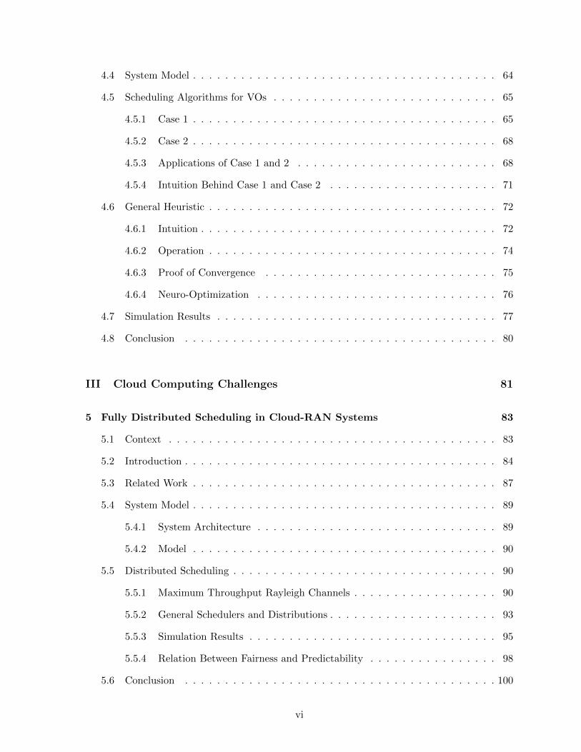
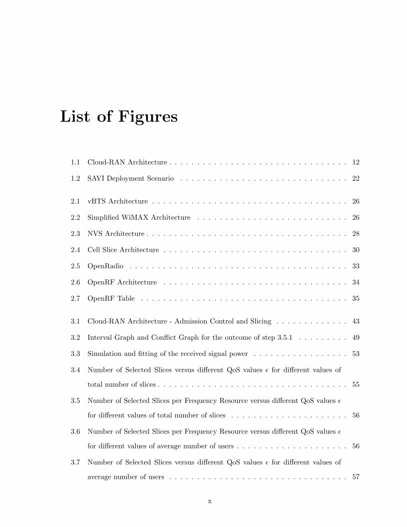
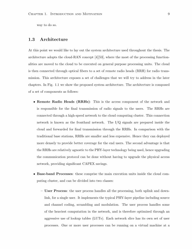
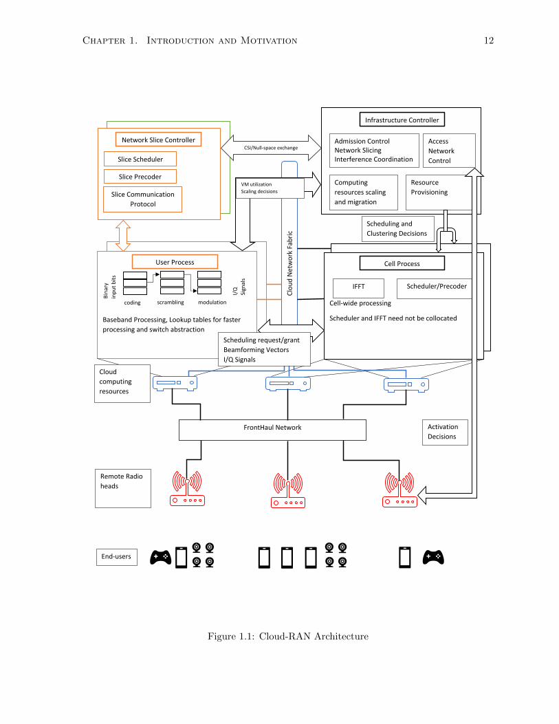
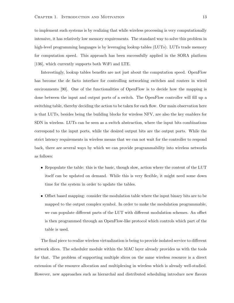
chapters. In Fig. 1.1 we show the proposed system architecture. The architecture is composed
of a set of components as follows:
• Remote Radio Heads (RRHs): This is the access component of the network and
is responsible for the final transmission of radio signals to the users. The RRHs are
connected through a high-speed network to the cloud computing cluster. This connection
network is known as the fronthaul network. The I/Q signals are prepared inside the
cloud and forwarded for final transmission through the RRHs. In comparison with the
traditional base stations, RRHs are smaller and less expensive. Hence they can deployed
more densely to provide better coverage for the end users. The second advantage is that
the RRHs are relatively agnostic to the PHY-layer technology being used, hence upgrading
the communication protocol can be done without having to upgrade the physical access
network, providing significant CAPEX savings.
• Base-band Processes: these comprise the main execution units inside the cloud com-
puting cluster, and can be divided into two classes:
– User Process: the user process handles all the processing, both uplink and down-
link, for a single user. It implements the typical PHY-layer pipeline including source
and channel coding, scrambling and modulation. The user process handles some
of the heaviest computation in the network, and is therefore optimized through an
aggressive use of lookup tables (LUTs). Each network slice has its own set of user
processes. One or more user processes can be running on a virtual machine at a
Chapter 1. Introduction and Motivation 10
time depending on the amount of computation needed and the capabilities of the
VM itself. The user process can be migrated to a different machine if the underlying
computing resource are insufficient. Hence, the concept of the user process is crucial
for realizing the cloud distributed computation model in the cloud-RAN architec-
ture. Unlike the typical cloud computing applications where the virtual machine is
the main computing in the system, the low latency required in wireless applications
raises the need for smaller computing units, represented here as the user and cell
processes.
– Cell Process: the cell process handles the processing that can not be done for each
user individually, but instead needs the data from all the users within a specific
cell/cluster. This includes for example the MAC-layer scheduling and the inverse
Fourier transform (IFFT) as well as the FFT operations. The cell process receives
the output of the user processes in the form of I/Q signals, and is responsible for
the final preparation of the signal sent to the access network through the fronthaul
connections. Being a cell wide process, the computation requirements of the cell
process are directly dependent on the number of users being served. Hence, it is
most computationally demanding when the traffic is at its peak. Even during low
traffic, the cell process is still computationally intensive, as the scheduler and IFFT
blocks are very computationally demanding. Similar to the user process, the cell
process might need to be migrated or have its VM upscaled as the computation
demand increases. However, there is another significant challenge in designing the
cell process due to the extensive traffic between the cell process and all the user
processes within the cell.
• Network Slice Controller: this includes all the control plane and higher-layers deci-
sions made by a specific slice. In essence, this corresponds to the core network within
the current network architectures, plus all the higher-layers operations. It also includes
the interface for communication with the infrastructure controller. The slice controller
communicates with the infrastructure controller about the admission control process, the
resource provisioning and the coordination between the different slices.
Chapter 1. Introduction and Motivation 11
• Infrastructure Controller: this is responsible for all the control decision regarding the
infrastructure itself, and the interaction between the network slices. It can be seen as the
generalization of the FlowVisors [120] used in wired network virtualization to the wireless
case. The infrastructure controller is responsible for the initial admission control and
slicing decisions, as well as provisioning this slicing during the normal network operation,
through scheduling and interference coordination for example. The infrastructure con-
troller is also responsible for administering the computing part of the network. Through
communication with the various processes, it can evaluate their computing needs and
carry out subsequent decisions for resource scaling or process migration.
1.4 Architecture Advantages
Having laid out the architecture, we can now discuss the challenges associated with deploying
it in practice. Within the cloud-RAN architecture, the cloud is responsible for handling all the
base-band processing required for transmission. Moving the base-band processing to the cloud
is challenging, due to two seemingly conflicting goals of cloud computing and wireless systems,
these are elasticity and latency. On one hand, a key concept within cloud computing is that of
elasticity, i.e. computing processes are virtualized and migrated between the physical servers
to optimize some criteria such as energy efficiency or utilization. On the other hand, migrating
virtual machines takes a few seconds to finish, which is three orders of magnitude more than
the millisecond latency required in modern wireless systems.
The Bell Labs architecture for C-RAN has addressed such a problem by introducing the
concepts of a user process and a cell process [53]. The user process handles all the processing
per a single user. User processes communicate with the cell process, which is responsible for
the cell-wide processing such as the scheduling and the last stages of the PHY-layer pipeline.
Through using a software process as the main processing unit instead of a virtual machine, the
issue with migration is solved, as what is needed now is just instantiating the process with the
same parameters on a different machine.
Another dimension of the problem is that building wireless systems on general purpose
CPUs is challenging due to the low-latency required in such systems. However, the key insight
Chapter 1. Introduction and Motivation 12
Baseband Processing, Lookup tables for faster
processing and switch abstraction
Baseband Processing, Lookup tables for faster
processing and switch abstraction
Baseband Processing, Lookup tables for faster
processing and switch abstraction
FrontHaul Network
coding scrambling modulation
Bin
ary
inp
ut
bit
s
I/Q
Sign
als
Cloud
computing
resources
Remote Radio
heads
Cell-wide processing
Scheduler and IFFT need not be collocated
User Process Cell Process
IFFT Scheduler/Precoder
Network Slice Controller
Slice Scheduler
Slice Communication
Protocol
Infrastructure Controller
Admission Control Network Slicing Interference Coordination
Computing
resources scaling
and migration
Resource
Provisioning
Clo
ud
Net
wo
rk F
abri
c
CSI/Null-space exchange
Slice Precoder VM utilization
Scaling decisions
Scheduling and
Clustering Decisions
Access
Network
Control
Activation
Decisions
Scheduling request/grant
Beamforming Vectors
I/Q Signals
End-users
Figure 1.1: Cloud-RAN Architecture
Chapter 1. Introduction and Motivation 13
to implement such systems is by realizing that while wireless processing is very computationally
intensive, it has relatively low memory requirements. The standard way to solve this problem in
high-level programming languages is by leveraging lookup tables (LUTs). LUTs trade memory
for computation speed. This approach has been successfully applied in the SORA platform
[136], which currently supports both WiFi and LTE.
Interestingly, lookup tables benefits are not just about the computation speed. OpenFlow
has become the de facto interface for controlling networking switches and routers in wired
environments [90]. One of the functionalities of OpenFlow is to decide how the mapping is
done between the input and output ports of a switch. The OpenFlow controller will fill up a
switching table, thereby deciding the action to be taken for each flow. Our main observation here
is that LUTs, besides being the building blocks for wireless NFV, are also the key enablers for
SDN in wireless. LUTs can be seen as a switch abstraction, where the input bits combinations
correspond to the input ports, while the desired output bits are the output ports. While the
strict latency requirements in wireless means that we can not wait for the controller to respond
back, there are several ways by which we can provide programmability into wireless networks
as follows:
• Repopulate the table: this is the basic, though slow, action where the content of the LUT
itself can be updated on demand. While this is very flexible, it might need some down
time for the system in order to update the tables.
• Offset based mapping: consider the modulation table where the input binary bits are to be
mapped to the output complex symbol. In order to make the modulation programmable,
we can populate different parts of the LUT with different modulation schemes. An offset
is then programmed through an OpenFlow-like protocol which controls which part of the
table is used.
The final piece to realize wireless virtualization is being to provide isolated service to different
network slices. The scheduler module within the MAC layer already provides us with the tools
for that. The problem of supporting multiple slices on the same wireless resource is a direct
extension of the resource allocation and multiplexing in wireless which is already well-studied.
However, new approaches such as hierarchal and distributed scheduling introduce new flavors
Chapter 1. Introduction and Motivation 14
into the problem.
1.5 Deployment Challenges
The deployment challenges can summarized around two design principles present in the archi-
tecture as follows:
• Cloud Computation Model:
– Distributed Processing: unlike the current systems where all the processing is
done centrally in the base station, the cloud computing model offers new challenges
due to the distributed nature of its resources, such as the virtual machines. The
split of the base-band processing into a user and a cell process is key here to leverage
the distributed computing model. However, a new challenge rises, which is how
to address the extensive communication traffic needed between these two types of
processes.
– Elastic Resources, Scaling and Clustering: the other major feature of the
cloud computing model is the resource elasticity and dynamic scaling of the assigned
resources based on the demand/traffic volume. First, there is the question of scaling
the computing resources according to the traffic pattern. This is one advantage of
the per-user processing approach used in the architecture, as it enables low-latency
scaling necessary for the wireless applications.
Second, a related question can be posed for the access network, in terms of the RRH
activation. Networks are typically designed according to the peak demand. When
the demand is outside its peak, then the cloud-RAN model calls for saving the
extra resources and utilizing the statistical multiplexing gains. Achieving resource
elasticity in the access network without affecting the quality of the service received
by the users is the key challenge here.
• Network Slicing and Infrastructure Sharing:
– Admission Control: One of the first decisions to be made by the infrastructure
controller is whether a new slice should be admitted in the network. This decision
Chapter 1. Introduction and Motivation 15
must take into account the available resources, the requested QoS as well as the QoS
of the slices already admitted. The infrastructure controller must ensure that the
QoS of the already admitted slices will not affected by the new slice. At the same
time, the infrastructure controller must ensure that it can provide the new slice
with its target QoS. This is particularly challenging in in the wireless domain due
to interference, the time-variable channel and the random movement and arrivals of
the network’s users.
– Slicing Dimension: Jointly with the admission control decision, the infrastructure
controller needs to decide which resources are assigned to this new slice, and which
dimensions (space,frequency,time) are used to slice the network. This decision re-
quires quantifying the performance difference between each slicing technique in terms
of the overall network utilization and the provided QoS.
– Resource Provisioning: once a slice has been admitted, the infrastructure con-
troller needs to provision its resources. The goal is to maintain its QoS from one
side, and guarantee a sufficient degree of isolation between it and the other slices
from the other side. This isolation is needed to protect the QoS of the other slices as
well. This process is done through scheduling and precoding as means of interference
coordination between the different slices.
1.6 Research Problems
The research problems we study in the thesis correspond directly to the deployment challenges
identified above. In particular:
• Network Slicing and Infrastructure Sharing:
– Admission Control: Several elements have to defined in order to answer the ad-
mission control question. These include a performance metric for the slice, i.e. QoS,
a multiplexing scheme and a coordination policy for resource provisioning. In wire-
less networks, QoS is directly related to the signal-to-noise ratio (SNR) and the
bandwidth. QoS is also function of the multiplexing scheme used. For example, if
Chapter 1. Introduction and Motivation 16
SDMA is used, then the QoS depends on the amount of spatial degrees of freedom
which in turn depend on the number of antennas given to a slice and its number of
users. Moreover, QoS is directly related to the number of RRHs and number of users
per RRH, which decides the portion of bandwidth each user can get. In summary,
a comprehensive QoS metric that takes into account both the PHY-layer aspects
(multiplexing scheme, SNR) and MAC-layer aspects (number of resource blocks per
user) is needed in order to arrive at an efficient admission control policy.
– Slicing Dimension: Several multiplexing schemes can be used to share the radio
spectrum between the slices, such as FDMA, SDMA and TDMA. Each scheme has
its own trade-offs, FDMA provides a good degree of isolation, while SDMA provides
more utilization efficiency. Moreover, one of the primary motivations for cloud-RAN
is leveraging the statistical multiplexing gains between the network slices to preserve
resources. A crucial ingredient in this case is the inclusion of the stochastic nature
of the number of active users. This randomness is key to modeling the statistical
multiplexing gains achieved by SDMA. To address the slicing problem, we need to
quantify the difference between the different schemes under study in terms of QoS,
isolation and statistical multiplexing.
– Resource Provisioning: Resources need to be provisioned by the infrastructure
controller in order to preserve the QoS performance for each slice. If spatial mul-
tiplexing is allowed between the slices, then an interference coordination policy has
to be imposed by the infrastructure owner to avoid excessive leakage or interference
between the slices. One example is the interference nulling policy. In this policy,
the infrastructure owner provides each slice with the null space upon which it must
project its signals to avoid interfering with the other slices.
Scheduling is another form of interference coordination focused on the frequency-time
resource blocks. Since the spectrum resources are now shared across different slices,
the typical MAC-layer scheduler is expanded into a two-stage hierarchal scheduler.
The first stage is where the slice schedules its own users, while the second stage
is where the scheduling of the slices themselves is undertaken by the infrastructure
Chapter 1. Introduction and Motivation 17
controller. However, a key question here is how can such a scheduler be designed
in a way that balances the flexibility given to the slice with the overall utilization
achievable by the infrastructure controller.
• Cloud Computation Model:
– Distributed Processing: The MAC-layer scheduler is a performance bottleneck in
the current systems. Migrating the system to the cloud will only increase the prob-
lem, as there is now the additional overhead due to the communication between the
user process and the cell process. Distributed scheduling is an interesting approach
in this case, as it lowers, or even eliminates, the excessive communication between
the user process and the cell process. A natural question to ask in this case is how
to design an effective distributed scheduler for the cloud-RAN, and how efficient can
this distributed scheduler be compared with the centralized one.
– Elastic Resources, Scaling and Clustering: The relatively cheap cost of RRHs
compared with traditional base stations enables building a denser wireless network.
This density leads to better coverage, but at the cost of increased energy usage
and interference. However, not all RRHs need to be active at the same time. An
important problem is how to select a subset of RRHs to be active at any point in
time such that overall network performance is not affected. Clustering is key in this
case, as interference is utilized, or at least eliminated, to provide satisfactory signal
levels for the affected users.
For the computing resources, wireless base band processing is a function of the
channel state, i.e. better channel conditions can support higher rates leading to
more extensive processing [136]. Hence, a good forecast model for the channel can be
used to also predict the needed computation power. This prediction can be provided
to the infrastructure controller which can then pro-actively make the scaling and
migration decisions for the cloud computing resources.
Chapter 1. Introduction and Motivation 18
1.7 Thesis Structure and Contributions
We have discussed some of the research problems in our architecture. Next we discuss how we
have addressed them in the thesis.
• Network Slicing and Infrastructure Sharing:
– Admission Control and Slicing: In Chapter 3, we study the admission control
and slicing problem. First, we provide a performance analysis comparing between
FDMA and SDMA. The random number of active users is integrated into the model
to account for statistical multiplexing. Then, a QoS metric is found based on the
null space projection technique. Third, a three-step algorithm is proposed for the
joint admission control and slicing decisions. Simulation results study the trade-off
between the QoS and the degree of multiplexing and correspondingly utilization.
This work has been published in [127].
– Resource Provisioning: In Chapter 4 we study the hierarchal scheduling as a form
of resource provisioning between the slices. The main assumption here is that the
infrastructure controller decision is limited to be a Yes/No decision to give the slice
the maximum flexibility. The problem is found to be an example of maximum weight
independent set (MWIS). First, we investigate two special cases that have polynomial
time optimum solutions. These cases correspond to the single carrier orthogonal
frequency division multiple access (SC-OFDMA) and time division multiple access
(TDMA). Then we investigate the intuition behind these cases optimality, and study
how we can extend this intuition by proposing a heuristic for the general case that
works well for the two special cases (98.5% and 94% respectively). This work has
been published in [126].
• Cloud Computation Model:
– Distributed Processing: In Chapter 5 we study the distributed scheduling prob-
lem. The approach is to completely remove the central scheduler and teach each
individual user process to come up with the decision on its own. We provide an
analytical performance analysis for the achievable rate in the case of the Rayleigh
Chapter 1. Introduction and Motivation 19
fading and maximum throughput scheduling. For this case, we find that the dis-
tributed scheduler can achieve 92% of the performance of the centralized one. Then,
we study more general scenarios employing machine learning clustering techniques
such as support vector machines (SVM) and decision trees. Here, we find that dis-
tributed scheduling is able to provide up to 89% of the performance of the centralized
one. We also uncover an interesting trade-off between the fairness of the scheduler
and its predictability, and study this trade-off for a general mean-variance scheduler.
This work has been published in [125].
– Elastic Resources, Scaling and Clustering: In Chapter 6 we study the problem
of joint activation and clustering in cloud-RANs. In this case, our objective function
is a combination of the number of active RRHs (representing the energy), the number
of users per active RRH and the SINR for these users (representing the QoS), and
the size of cluster (representing the clustering penalty). Our main constraint is a
coverage constraint, where each user has to be covered by at least one RRH. We
propose a two step algorithm to handle the problem. The first step is a set-cover
problem where the minimum number of RRHs is activated to guarantee coverage.
The second step is a greedy improvement by activating more RRHs or clustering
active ones to improve performance. This work has been published in [128].
This framework is then extended in Chapter 7 in several directions. First we include
the user-RRH association as another variable in our model. Second, we expand the
problem to a long-term optimization where the queuing dynamics are integrated into
the model. The resulting problem is an example of signomial optimization, which is
then solved efficiently using successive geometric approximation. Finally, we study
how this framework can be extended into a stochastic control framework by operating
on the traffic forecast. We measure the sensitivity of our decisions with respect to
the traffic forecast error, and find it to be 9% for the activation decision and 18%
for the clustering decision.
In Chapter 8 and 9 we study the scaling of computing resources jointly with anomaly
detection. Chapter 8 is focused on identifying a good set of features for identifying
Chapter 1. Introduction and Motivation 20
anomalies 1. The main framework is then studied in Chapter 9 where we study the
joint problem of computing resource scaling and anomaly detection. This is modeled
as a stochastic optimization problem. The proposed solution policy is based on a
Gaussian process model where the probability of exceeding a utilization threshold is
our scaling indicator, and the deviation between the prediction and the measurement
is our anomaly detector. We measure a prediction accuracy of 95% and an anomaly
detection accuracy of over 90%. Part of this work has been published in [145].
1.8 NFV, SDN and VN within the Context of Wireless Virtu-
alization
Applying the concepts of NFV, SDN and VN to wireless networks necessitates the specification
of the aspects of architecture, design and implementation of wireless virtualization. In this sec-
tion , we summarize our previous discussion by revisiting the motivations behind these concepts.
We see that NFV is about avoiding the use of specialized HW, SDN is about programmability
and VN is about sharing the resources between different slices.
1.8.1 NFV in Wireless
Traditionally, wireless systems have been implemented using FPGAs or ASIIC to accommodate
the high computational requirements of the wireless PHY and MAC layers. However, the
continuous advancements in CPUs and the powerful capabilities of data centers have made it
possible to build such systems using only general purpose CPUs. While wireless protocols have
high computational needs, their memory needs are relatively low. We can see then that the use
of look up tables (LUT) is fundamental for any implementation of wireless systems on CPUs.
LUT trade memory for computation, and have been successfully used to implement WiFi on
general purpose CPUs in SORA [136].
1Chapter 8 is a joint work with Joseph Wahba, a former MSc student in the research group.
Chapter 1. Introduction and Motivation 21
1.8.2 SDN in Wireless
In wired SDN, the OpenFlow controller will fill up a switching table which decides the action
to be taken for each flow. Our main observation is that LUTs are the key enablers for SDN
in wireless as they are for NFV. LUTs can be seen as a switch abstraction, where the input
bits combinations correspond to the input ports, and the desired output bits correspond to the
output ports.
1.8.3 VN in Wireless
For the radio access network, the problem of slicing the spectrum between a set of virtual
networks is equivalent to the well known multiplexing problem. While the standard approaches
such FDMA, TDMA, CDMA and SDMA are still applicable, new approaches such as hierarchal
and distributed scheduling introduce new flavors into the problem.
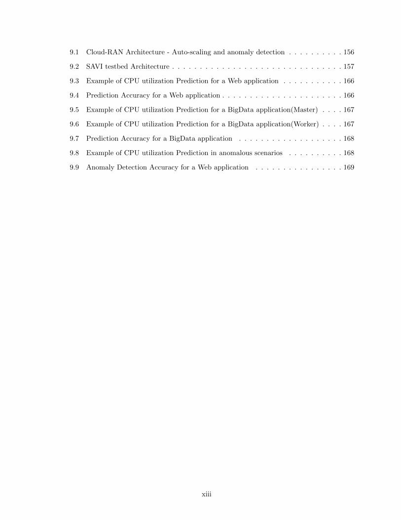
1.9 Deployment Scenario
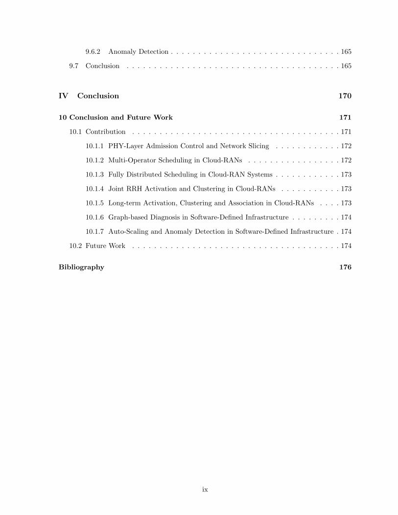
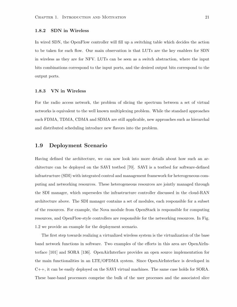
Having defined the architecture, we can now look into more details about how such an ar-
chitecture can be deployed on the SAVI testbed [70]. SAVI is a testbed for software-defined
infrastructure (SDI) with integrated control and management framework for heterogeneous com-
puting and networking resources. These heterogeneous resources are jointly managed through
the SDI manager, which supersedes the infrastructure controller discussed in the cloud-RAN
architecture above. The SDI manager contains a set of modules, each responsible for a subset
of the resources. For example, the Nova module from OpenStack is responsible for computing
resources, and OpenFlow-style controllers are responsible for the networking resources. In Fig.
1.2 we provide an example for the deployment scenario.
The first step towards realizing a virtualized wireless system is the virtualization of the base
band network functions in software. Two examples of the efforts in this area are OpenAirIn-
terface [101] and SORA [136]. OpenAirInterface provides an open source implementation for
the main functionalities in an LTE/OFDMA system. Since OpenAirInterface is developed in
C++, it can be easily deployed on the SAVI virtual machines. The same case holds for SORA.
These base-band processors comprise the bulk of the user processes and the associated slice
Chapter 1. Introduction and Motivation 22
SDI Manager
Cloud-RAN Module
OpenStack
Nova Module
Admission
module
Scheduling
module
Scaling
module
QoS request
Users count estimation
Slice Controller
Precoder Design
User Process
Updating the
LUT
Querying the
spatial resources
Distributed scheduling
Hierarchal scheduling
Cell Process
Updating the
scheduling
weights CSI report
Migration/scaling
Figure 1.2: SAVI Deployment Scenario
controller.
The second step is to interface the wireless network, i.e. OpenAirInterface with the SDI
manager. This connection is crucial to realize the architecture and solutions discussed above.
From the communications and networking perspective, the SDI manager should be able
to control and update the PHY-layer pipeline through the LUT entries. LUTs provide an
abstraction of the PHY-layer processing similar to the flow processing used in OpenFlow, hence
similar control mechanisms can be developed to control the PHY-layer operation. Besides
choosing the appropriate modulation and coding schemes, the SDI manager can update the
precoding LUTs in the PHY-layer pipeline in accordance with the null space projection policy
to ensure elimination of inter-slice interference.
From the computing perspective, the main observation is that the computing needs of a
wireless system are related to the CSI [136]. Better channel conditions are utilized for higher
transmission rates and consequently more processing needs. By providing the CSI to the cloud
controller, and with appropriate forecast mechanisms, the VMs scaling and migrations decisions
Chapter 1. Introduction and Motivation 23
can be found and executed pro-actively in an efficient manner.
Chapter 2
Background and Literature Review
2.1 A First Look at Wireless Virtualization
Wireless virtualization, in the broadest sense, can be considered as a multiple-access problem
between the virtual operators who share the same infrastructure and access the same part of
the spectrum. This view has been taken in the GENI document on wireless virtualization[106],
which discusses the basic multiple access techniques as approaches to wireless virtualization.
These multiple access techniques are
• Frequency Division Multiple Access (FDMA).
• Time Division Multiple Access (TDMA).
• Code Division Multiple Access (CDMA).
• Space Division Multiple Access (SDMA).
• Any combination of the above techniques.
There are of course trade-offs in taking each approach. FDMA can result in low utilization of
the scarce spectrum resource and can be infeasible when the spectrum band is crowded. TDMA
alleviates this utilization problem but suffers from context-switching delay which can be in the
order of milliseconds. The SDMA approach taken in the ORBIT testbed [115] is not feasible
in practical commercial networks. CDMA, while not having the limitations above, is known to
be interference-limited as in current cellular architectures.
24
Chapter 2. Background and Literature Review 25
2.2 Literature Review
This section covers the efforts by the research community into building virtualized wireless
networks. These efforts can be classified into the following categories:
• WiMAX virtualization.
• LTE virtualization.
• Resource Abstraction and dynamic resource allocation.
2.2.1 WiMAX Virtualization
Many of the key papers within the framework of wireless virtualization were published by the
team at Rutgers University in joint effort with NEC Labs. These efforts were targeted at the
WiMAX system, and had the advantage of performing real tests within their ORBIT testbed
[115]. Their work has resulted in the following virtualization architectures:
1. vBTS: virtualization through emulation of base stations.
2. NVS: virtualization through MAC-layer enhancements.
3. CellSlice: virtualization through feedback control.
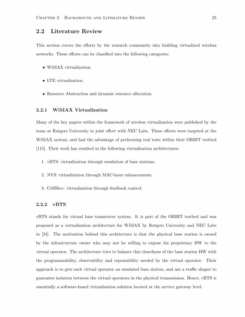
2.2.2 vBTS
vBTS stands for virtual base transceiver system. It is part of the ORBIT testbed and was
proposed as a virtualization architecture for WiMAX by Rutgers University and NEC Labs
in [24]. The motivation behind this architecture is that the physical base station is owned
by the infrastructure owner who may not be willing to expose his proprietary HW to the
virtual operator. The architecture tries to balance this closedness of the base station HW with
the programmability, observability and repeatability needed by the virtual operator. Their
approach is to give each virtual operator an emulated base station, and use a traffic shaper to
guarantee isolation between the virtual operators in the physical transmission. Hence, vBTS is
essentially a software-based virtualization solution located at the service gateway level.
Chapter 2. Background and Literature Review 26
Physical BTS
vBTS 1
vBTS 2
User in VN1
User in VN2
Isolation
Figure 2.1: vBTS Architecture
BST2
BTS1
BTS3
ASN CSNContent
Providers
Local IP network
Internet
Figure 2.2: Simplified WiMAX Architecture
Chapter 2. Background and Literature Review 27
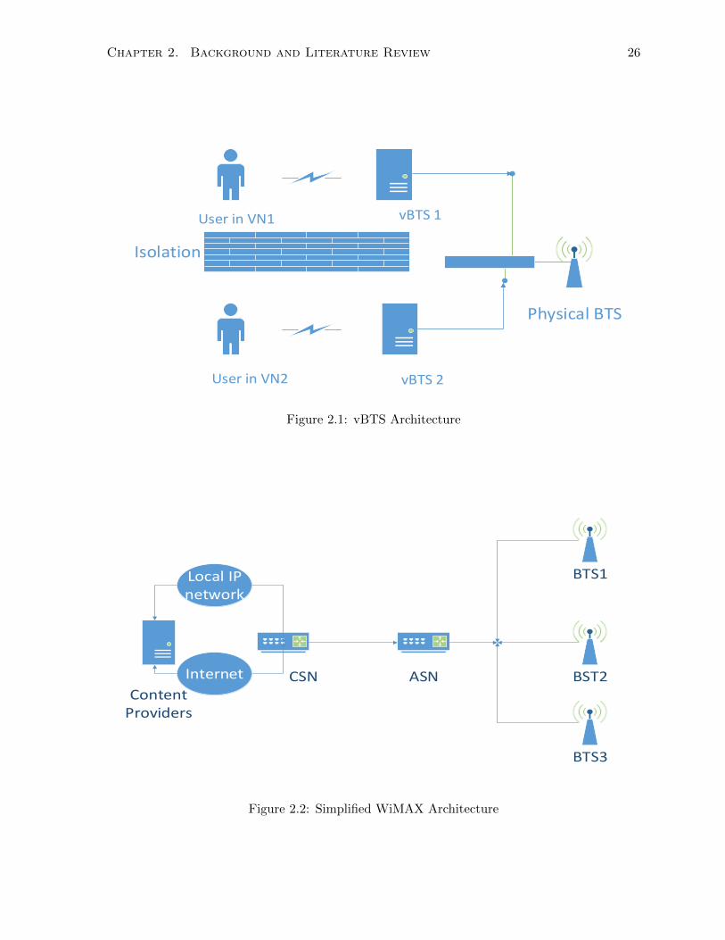
The basic WiMAX architecture is shown in Fig. 2.2. The main components of the archi-
tecture are the base transceiver system (BTS), the access service network gateway (ASN), and
the connectivity service network gateway (CSN). The ASN gateway is the connection between
the BTS and the access core network. The vBTS architecture emulates different base stations
for the different virtual operators in VMs running within a data center. One major advantage
of vBTS is that it gives each slice complete control over its MAC, enabling the slice to support
different MACs each belonging to a specific slice. The data center is connected through the
ASN gateway to the BTS. Hence, it falls down to the ASN gateway to guarantee the isola-
tion between the traffic belonging to different vBTSs. This is done through the Slice Isolation
Engine (SIE), which is an amendment to the standard ASN gateway.
The SIE is implemented through a virtual network traffic shaper (VNTS) mechanism pro-
posed in [23]. This is a dynamic traffic sharping technique aimed at balancing utilization and
isolation. The mechanism is divided into the VNTS engine and the VNTS controller. The
VNTS controller interacts with the physical base station through the simple network manage-
ment protocol (SNMP) in order to get information about the conditions of the base station
and prevent overflowing it with packets beyond its transmission capacity. Once aware of the
physical base station transmission capacity and of the wights given to each virtual operator,
it enforces the traffic shaping through the VNTS engine according to the wight given to each
slice without exceeding the capacity of the base station.
While vBTS provides a simple solution to the virtualization problem, it has its own draw-
backs. First, it can only isolate traffic in the downlink as it has no control over the uplink.
Moreover, the SIE can only provide coarse rather than strict isolation between the slices. Third,
the existence of two scheduling modules, one at the physical base station and one at SIE affects
the utilization of the system since they are not fully coordinated.
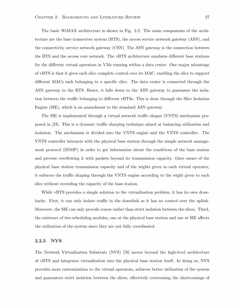
2.2.3 NVS
The Network Virtualization Substrate (NVS) [76] moves beyond the high-level architecture
of vBTS and integrates virtualization into the physical base station itself. In doing so, NVS
provides more customization to the virtual operators, achieves better utilization of the system
and guarantees strict isolation between the slices, effectively overcoming the shortcomings of
Chapter 2. Background and Literature Review 28
Frame Scheduler
Classifier
Slice 1 Slice 2 Slice 3
DownLink two-level scheduler
Uplink two-level scheduler
DL Flows
UL Flows
Figure 2.3: NVS Architecture
the vBTS architecture. NVS also has control over both the uplink and downlink unlike vBTS.
The design principles of NVS are summarized as follows:
1. Isolation: between slices.
2. Customization: for each individual slice.
3. Utilization: efficient resource usage.
Even though NVS is designed for WiMAX, it can be easily extended to other orthogonal fre-
quency division multiple-access (OFDMA) based systems such as Long Term Evolution (LTE)
and LTE-Advanced.
Virtualization Level
WiMAX defines the notion of a service flow between the base station and a user device. A
service flow is a unidirectional flow (either uplink or downlink) of packets with a particular set
of QoS parameters. A user’s end-to-end connections are mapped to one or more of its service
flows. The setup of service flows is left as a policy specification to the network operators. For
efficient resource allocation, the base station includes a collection of schedulers. A downlink flow
scheduler determines the sequence of packets to be transmitted in the downlink direction based
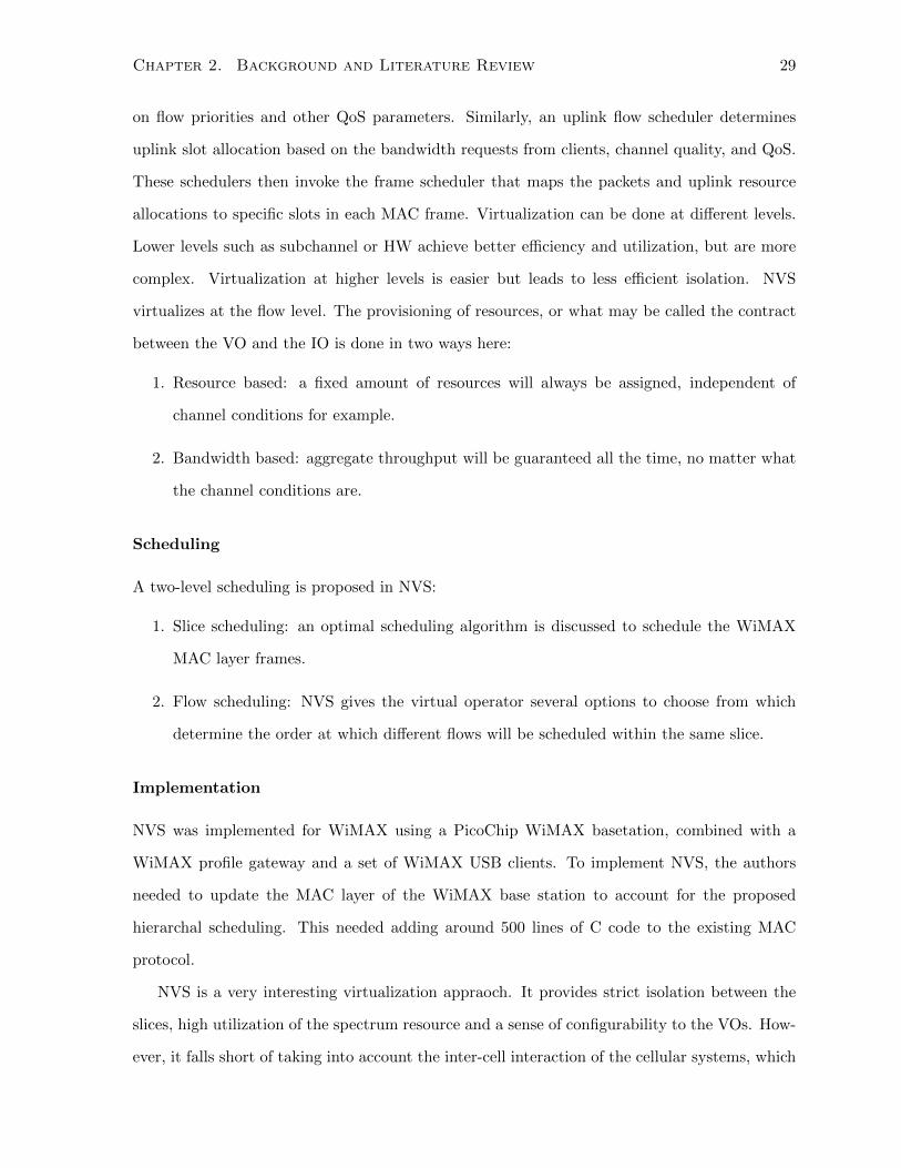
Chapter 2. Background and Literature Review 29
on flow priorities and other QoS parameters. Similarly, an uplink flow scheduler determines
uplink slot allocation based on the bandwidth requests from clients, channel quality, and QoS.
These schedulers then invoke the frame scheduler that maps the packets and uplink resource
allocations to specific slots in each MAC frame. Virtualization can be done at different levels.
Lower levels such as subchannel or HW achieve better efficiency and utilization, but are more
complex. Virtualization at higher levels is easier but leads to less efficient isolation. NVS
virtualizes at the flow level. The provisioning of resources, or what may be called the contract
between the VO and the IO is done in two ways here:
1. Resource based: a fixed amount of resources will always be assigned, independent of
channel conditions for example.
2. Bandwidth based: aggregate throughput will be guaranteed all the time, no matter what
the channel conditions are.
Scheduling
A two-level scheduling is proposed in NVS:
1. Slice scheduling: an optimal scheduling algorithm is discussed to schedule the WiMAX
MAC layer frames.
2. Flow scheduling: NVS gives the virtual operator several options to choose from which
determine the order at which different flows will be scheduled within the same slice.
Implementation
NVS was implemented for WiMAX using a PicoChip WiMAX basetation, combined with a
WiMAX profile gateway and a set of WiMAX USB clients. To implement NVS, the authors
needed to update the MAC layer of the WiMAX base station to account for the proposed
hierarchal scheduling. This needed adding around 500 lines of C code to the existing MAC
protocol.
NVS is a very interesting virtualization appraoch. It provides strict isolation between the
slices, high utilization of the spectrum resource and a sense of configurability to the VOs. How-
ever, it falls short of taking into account the inter-cell interaction of the cellular systems, which
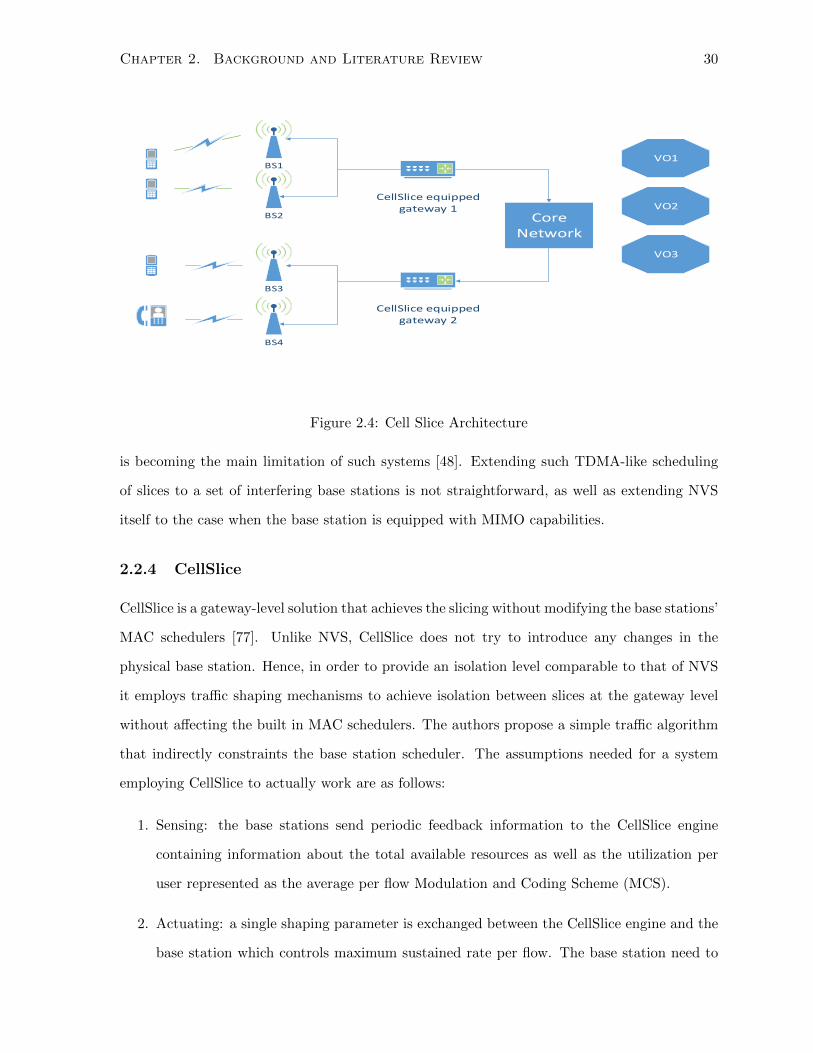
Chapter 2. Background and Literature Review 30
BS1
BS2
BS3
BS4
CellSlice equipped gateway 1
CellSlice equipped gateway 2
Core Network
VO1
VO2
VO3
Figure 2.4: Cell Slice Architecture
is becoming the main limitation of such systems [48]. Extending such TDMA-like scheduling
of slices to a set of interfering base stations is not straightforward, as well as extending NVS
itself to the case when the base station is equipped with MIMO capabilities.
2.2.4 CellSlice
CellSlice is a gateway-level solution that achieves the slicing without modifying the base stations’
MAC schedulers [77]. Unlike NVS, CellSlice does not try to introduce any changes in the
physical base station. Hence, in order to provide an isolation level comparable to that of NVS
it employs traffic shaping mechanisms to achieve isolation between slices at the gateway level
without affecting the built in MAC schedulers. The authors propose a simple traffic algorithm
that indirectly constraints the base station scheduler. The assumptions needed for a system
employing CellSlice to actually work are as follows:
1. Sensing: the base stations send periodic feedback information to the CellSlice engine
containing information about the total available resources as well as the utilization per
user represented as the average per flow Modulation and Coding Scheme (MCS).
2. Actuating: a single shaping parameter is exchanged between the CellSlice engine and the
base station which controls maximum sustained rate per flow. The base station need to
Chapter 2. Background and Literature Review 31
take this parameter into consideration when performing its MAC scheduling.
The operation of CellSlice is simple, whenever a base station indicates that it is under-
utilized, CellSlice incrementally increases the maximum sustainable rate for all users. This
continues until the base station indicates over utilization, after which CellSlice must reset the
maximum sustainable rate for each flow according to its service level agreement with the VO
owning such a flow.
While CellSlice offers a very simple solution for wireless virtualization that introduces no
changes to the physical base station, its performance is limited by the traffic characteristics of
the flows. Specifically, the more fluctuating the traffic is, the harder it becomes to control it
through CellSlice feedback loop. The drawback is more explicit in the uplink, where CellSlice
engine is not aware of the state of the flows until the base station sends its periodic feedback
messages. In order to guarantee strict isolation between the slices, the base station needs to send
its feedback messages more frequently, introducing a trade-off between isolation and utilization.
2.2.5 LTE eNB Virtualization
As part of the 4WARD project in EU, the research group at University of Bremen has considered
virtualization of the LTE eNB [159]. Their virtualization framework of the LTE eNB consists
of two main stages:
1. Virtualization of the physical HW of the eNB,
2. Virtualization of the air interface controlled by the eNB.
The authors focused on the virtualization of air interface, considered the physical node
virtualization to be a task similar to any other computing node virtualization. An entity
called ”Hypervisor” will be responsible for scheduling the physical resources between the virtual
instances running on top of it.
The hypervisor is also responsible for scheduling the air interface resources. Since we are
dealing with LTE, the smallest unit of air interface that can be allocated is the Physical Resource
Block (PRB), the task of the hypervisor is to schedule access to the PRBs between different
virtual operators.
Chapter 2. Background and Literature Review 32
Framework
The architecture is similar to the NVS architecture proposed for WiMAX. One difference is the
assumption that the each virtual operator can have his own virtual eNB, e.g. software based
eNB running on a VM. Another difference is that their scheduling is slightly different than
NVS in that it schedules the users belonging to the different virtual operators directly instead
of scheduling the slices.
Methodology
Collect information from the virtual operators about their users, such as channel conditions,
then, depending on the type of contract of the virtual operators, the PRBs are allocated.
Types of Contracts
The authors considered four types of contracts, i.e. SLAs, between the IO and the VOs
• Fixed Guarantee: fixed BW will be allocated all the time.
• Dynamic Guarantees: a guaranteed maximum BW will be allocated if requested, other-
wise only the actually needed BW is allocated.
• Best Effort with min guarantees: minimum guaranteed BW will be allocated all the time,
and extra BW may be allocated in a best-effort manner.
• Best Effort with no guarantees: BW will be allocated in a best-effort manner only.
The authors then proposed a scheduling algorithm for allocating the PRBs among virtual
operators taking into account the types of contracts used. This framework follows a mixed
TDMA/FDMA approach, which is limited by the switching times of TDMA, and the maximum
number of subcarriers (FDMA).
2.2.6 SDR and Virtualization
Another line of work has concerned itself with virtualization architectures that work in a way
very similar to the software-defined radio (SDR) architectures. These include OpenRadio and
OpenRF.
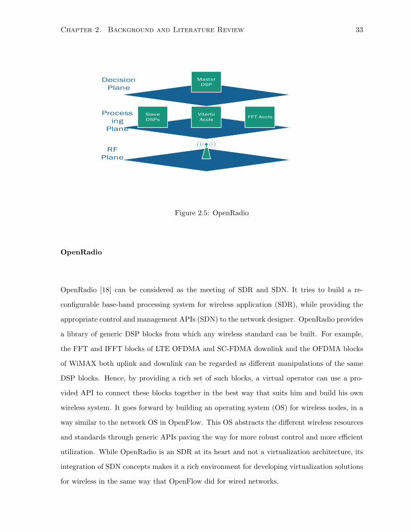
Chapter 2. Background and Literature Review 33
Master
DSP
Slave
DSPs
Viterbi
AcclsFFT Accls
Decision
Plane
Process
ing
Plane
RF
Plane
Figure 2.5: OpenRadio
OpenRadio
OpenRadio [18] can be considered as the meeting of SDR and SDN. It tries to build a re-
configurable base-band processing system for wireless application (SDR), while providing the
appropriate control and management APIs (SDN) to the network designer. OpenRadio provides
a library of generic DSP blocks from which any wireless standard can be built. For example,
the FFT and IFFT blocks of LTE OFDMA and SC-FDMA downlink and the OFDMA blocks
of WiMAX both uplink and downlink can be regarded as different manipulations of the same
DSP blocks. Hence, by providing a rich set of such blocks, a virtual operator can use a pro-
vided API to connect these blocks together in the best way that suits him and build his own
wireless system. It goes forward by building an operating system (OS) for wireless nodes, in a
way similar to the network OS in OpenFlow. This OS abstracts the different wireless resources
and standards through generic APIs paving the way for more robust control and more efficient
utilization. While OpenRadio is an SDR at its heart and not a virtualization architecture, its
integration of SDN concepts makes it a rich environment for developing virtualization solutions
for wireless in the same way that OpenFlow did for wired networks.
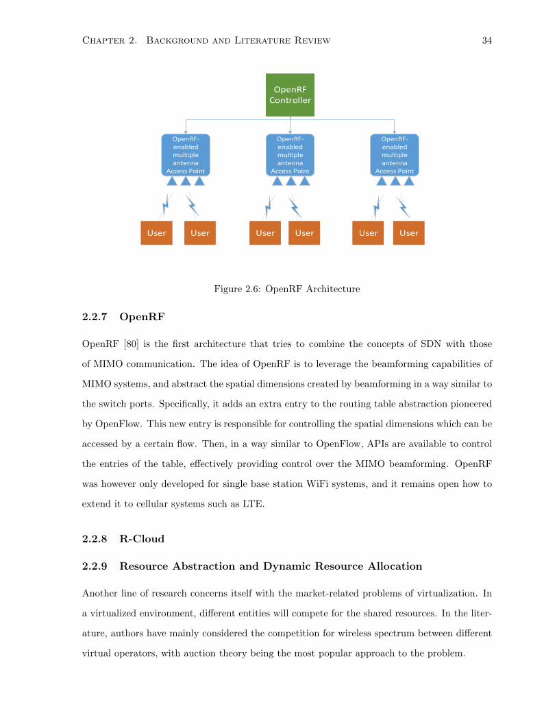
Chapter 2. Background and Literature Review 34
OpenRF Controller
OpenRF-enabled multiple antenna
Access Point
OpenRF-enabled multiple antenna
Access Point
OpenRF-enabled multiple antenna
Access Point
User User User User User User
Figure 2.6: OpenRF Architecture
2.2.7 OpenRF
OpenRF [80] is the first architecture that tries to combine the concepts of SDN with those
of MIMO communication. The idea of OpenRF is to leverage the beamforming capabilities of
MIMO systems, and abstract the spatial dimensions created by beamforming in a way similar to
the switch ports. Specifically, it adds an extra entry to the routing table abstraction pioneered
by OpenFlow. This new entry is responsible for controlling the spatial dimensions which can be
accessed by a certain flow. Then, in a way similar to OpenFlow, APIs are available to control
the entries of the table, effectively providing control over the MIMO beamforming. OpenRF
was however only developed for single base station WiFi systems, and it remains open how to
extend it to cellular systems such as LTE.
2.2.8 R-Cloud
2.2.9 Resource Abstraction and Dynamic Resource Allocation
Another line of research concerns itself with the market-related problems of virtualization. In
a virtualized environment, different entities will compete for the shared resources. In the liter-
ature, authors have mainly considered the competition for wireless spectrum between different
virtual operators, with auction theory being the most popular approach to the problem.
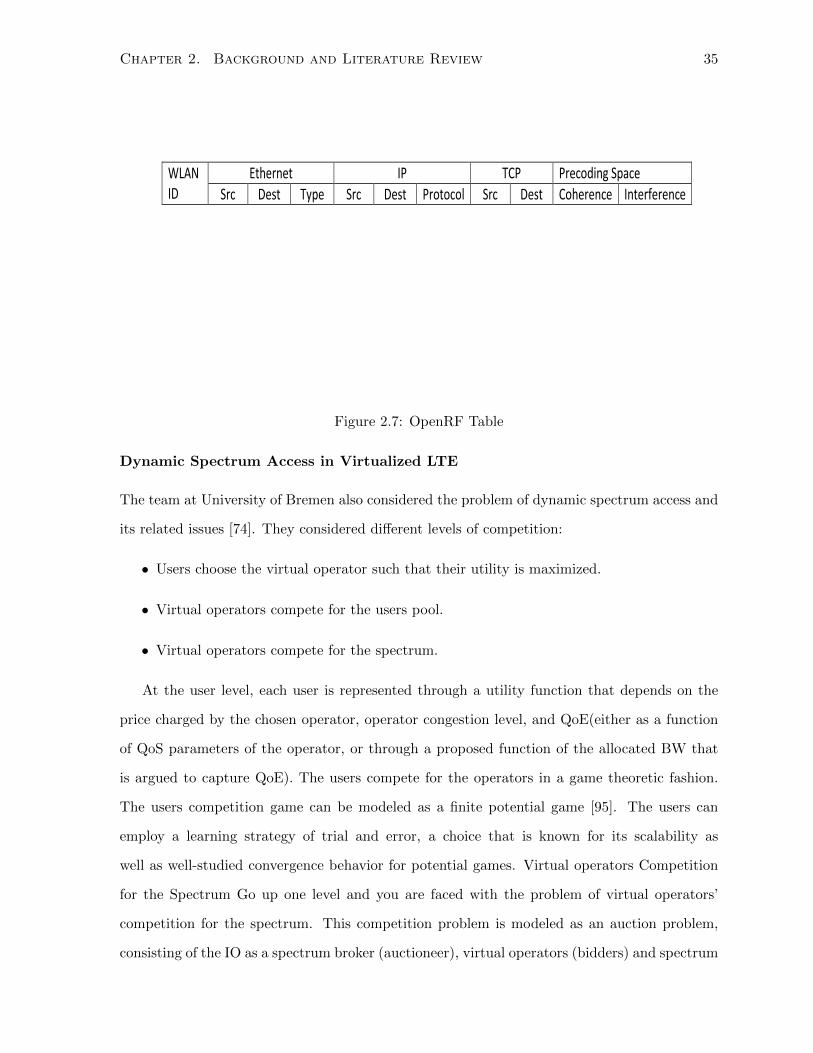
Chapter 2. Background and Literature Review 35
WLAN ID
Ethernet IP TCP Precoding Space
Src Dest Type Src Dest Protocol Src Dest Coherence Interference
Figure 2.7: OpenRF Table
Dynamic Spectrum Access in Virtualized LTE
The team at University of Bremen also considered the problem of dynamic spectrum access and
its related issues [74]. They considered different levels of competition:
• Users choose the virtual operator such that their utility is maximized.
• Virtual operators compete for the users pool.
• Virtual operators compete for the spectrum.
At the user level, each user is represented through a utility function that depends on the
price charged by the chosen operator, operator congestion level, and QoE(either as a function
of QoS parameters of the operator, or through a proposed function of the allocated BW that
is argued to capture QoE). The users compete for the operators in a game theoretic fashion.
The users competition game can be modeled as a finite potential game [95]. The users can
employ a learning strategy of trial and error, a choice that is known for its scalability as
well as well-studied convergence behavior for potential games. Virtual operators Competition
for the Spectrum Go up one level and you are faced with the problem of virtual operators’
competition for the spectrum. This competition problem is modeled as an auction problem,
consisting of the IO as a spectrum broker (auctioneer), virtual operators (bidders) and spectrum
Chapter 2. Background and Literature Review 36
(auctioned items). Uniform price auctions are chosen as the auction framework. By choosing
suitable utility functions for the auctioneer and the virtual operators, and from the properties
of uniform price auctions, the authors were able to prove the existence of a dominant strategy
for virtual operators. The auction process goes as follows:
1. The auctioneer announces the start of the auction and the time to submit the bids.
2. Each bidder observes the demands of its own users.
3. Bidders submit their bids.
4. The auctioneer receives the bids and decides the shares of each virtual operator.
5. The allocations are fed to the hypervisor which takes the role of scheduling.
The authors however fell short of studying the case when the two games are interwound.
Stochastic Game for Wireless Virtualization
Game theory has been used in [45] to model the interaction between the different entities
in a virtualized wireless network. This paper provides a novel framework for virtualization
through resource abstraction. The motivation for this approach was that previous approaches to
virtualization require the service providers to explicitly understand the wireless access protocols.
Their new approach alleviates that by separating the wireless resource management performed
at the IO level from the quality-of-service control performed at the virtual operator level.
Moreover, by having the infrastructure provider take control of the resource management, it
is more aware of the heterogeneous services and the underlying time-varying wireless features
(e.g., channel conditions, available spectrum resources).
In such a framework, each virtual operator has a certain utility, which is the sum of the
utilities of its own users. The utility of each user is a function of the rate allocated to it, as
part of the feasible rate region(the possible set of rates given a certain channel). The virtual
operators bid for the wireless resources in the form of rates on behalf of their users. The
VickreyClarkeGroves is chosen as the bidding mechanism used by the virtual operators to bid
for the spectrum. The competitive game between virtual operators is played in sequential

Chapter 2. Background and Literature Review 37
stages, and the utility is considered to be the average utility through all stages. The main
results of this paper are summarized as follows:
1. Modeling the game as a stochastic game.
2. Proving the existence of NE in the game.
3. Using conjectural prices, the sequential games are decoupled and the game is tractable.
4. Centralized algorithm for finding the conjectural prices by the infrastructure operator.
5. Proving the efficiency of the NE associated with these prices.
6. Use of reinforcement learning to overcome the non-causality of the problem.
Part II
Network Slicing and Infrastructure
Sharing
38
39
In this part, we study a set of challenges related to the admission and multiplexing of
several network slices on the same physical infrastructure. These challenges revolve around
admission control, network slicing and resource provisioning. First, we study the admission
control problem from the perspective of the infrastructure controller. We also study the QoS
performance of the different multiplexing schemes and how they can be used in the admission
control decisions. In relation to the admission control, we study the resource provisioning
policies by which the infrastructure controller can maintain an appropriate QoS performance
for the admitted slices. We study two forms of resource provisioning, the first is precoding-based
interference coordination and the second is hierarchal scheduling.
Chapter 3
PHY-Layer Admission Control and
Network Slicing
3.1 Context
Wireless virtualization is a promising approach to foster innovation and prevent the ossification
of wireless networks. Within a virtualized wireless network, multiple network slices, or virtual
operators (VO), are co-hosted on the same physical infrastructure. In this chapter, we study
one of the first decisions that need to be taken by the infrastructure controller, that is which
slices should be admitted into the physical infrastructure and how should the network be sliced
between them, i.e. which multiplexing technique, TDMA, FDMA or SDMA, should be used.
Another related question is how should the stochastic arrival process affect the slicing and QoS
criteria. To answer these two questions, we study the problem of QoS-aware joint admission
control and network slicing. Due to the NP-hardness of the problem, we approach it using a
heuristic algorithm composed of three steps: spectrum allocation, admission control and spatial
multiplexing. The proposed algorithm incorporates the effects of QoS and stochastic traffic. We
study through simulations the benefits of joint spatial-frequency multiplexing over the static
frequency slicing approach. Finally, our simulation results help shed some light on the trade-offs
between frequency and spatial multiplexing as well as between QoS and utilization.
40
Chapter 3. PHY-Layer Admission Control and Network Slicing 41
3.2 Introduction
Current cellular networks are plagued with long installation times, high cost of equipment and
the widespread use of specialized hardware. The tight association between the hardware and
its functionalities is an obstacle in front of fast paced innovation. These issues have encouraged
the introduction of virtualization principles into the wireless domain [32]. Virtualization essen-
tially involves three design principles: the use of modular hardware (HW) to support arbitrary
software (SW) functionalities; support multiple networks on the same physical infrastructure;
and use of SW to manage, control and upgrade the different resource slices [75]. In this regard,
C-RAN has appeared as a promising architecture for 5G networks leveraging the concepts of
wireless virtualization [4].
The problem of wireless virtualization can not be studied without considering the PHY-
layer aspects of it, as this is a main differentiator between wireless and wired networks. Due
to the stochastic nature of the wireless channel and the scarcity of the spectrum, we have to
adopt an admission control step that decides whether the wireless channel/network has enough
capacity to serve a specific network slice. Together with the admission control step, there is
also the question of how should the new slice be admitted. Such question does not show up in
the wired network since the virtualization is done at the packet level. However, since the radio
spectrum is shared between all slices, studying wireless virtualization involves delving deeper
into how the spectrum should be shared and how the capacity is divided between the slices.
Moreover, this study must also take into account the stochastic nature of the network traffic
and leverage the resulting statistical multiplexing gains. Jointly with all these decisions, the
infrastructure controller must decide upon the provisioning policy between the slices once they
have been admitted.
A challenge unique to wireless environments is how to share the air interface between the
slices and which multiplexing scheme should be used. The qualitative understanding is that
FDMA provides the best isolation and is the most practical, however it might result in under-
utilization due to the loss of statistical multiplexing gain [3]. TDMA is adaptive to the varying
traffic behavior, but suffers from synchronization and switching time issues [3]. SDMA is the
most flexible yet also the most complex. However, quantitatively characterizing the difference
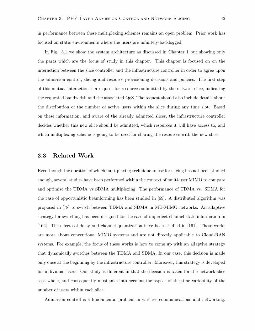
Chapter 3. PHY-Layer Admission Control and Network Slicing 42
in performance between these multiplexing schemes remains an open problem. Prior work has
focused on static environments where the users are infinitely-backlogged.
In Fig. 3.1 we show the system architecture as discussed in Chapter 1 but showing only
the parts which are the focus of study in this chapter. This chapter is focused on on the
interaction between the slice controller and the infrastructure controller in order to agree upon
the admission control, slicing and resource provisioning decisions and policies. The first step
of this mutual interaction is a request for resources submitted by the network slice, indicating
the requested bandwidth and the associated QoS. The request should also include details about
the distribution of the number of active users within the slice during any time slot. Based
on these information, and aware of the already admitted slices, the infrastructure controller
decides whether this new slice should be admitted, which resources it will have access to, and
which multiplexing scheme is going to be used for sharing the resources with the new slice.
3.3 Related Work
Even though the question of which multiplexing technique to use for slicing has not been studied
enough, several studies have been performed within the context of multi-user MIMO to compare
and optimize the TDMA vs SDMA multiplexing. The performance of TDMA vs. SDMA for
the case of opportunistic beamforming has been studied in [69]. A distributed algorithm was
proposed in [78] to switch between TDMA and SDMA in MU-MIMO networks. An adaptive
strategy for switching has been designed for the case of imperfect channel state information in
[162]. The effects of delay and channel quantization have been studied in [161]. These works
are more about conventional MIMO systems and are not directly applicable to Cloud-RAN
systems. For example, the focus of these works is how to come up with an adaptive strategy
that dynamically switches between the TDMA and SDMA. In our case, this decision is made
only once at the beginning by the infrastructure controller. Moreover, this strategy is developed
for individual users. Our study is different in that the decision is taken for the network slice
as a whole, and consequently must take into account the aspect of the time variability of the
number of users within each slice.
Admission control is a fundamental problem in wireless communications and networking.
Chapter 3. PHY-Layer Admission Control and Network Slicing 43
Baseband Processing, Lookup tables for faster
processing and switch abstraction
Baseband Processing, Lookup tables for faster
processing and switch abstraction
FrontHaul Network
coding scrambling modulation
Bin
ary
inp
ut
bit
s
I/Q
Sign
als
Cloud
computing
resources
Remote Radio
heads
User Process
Network Slice Controller
Slice Communication
Protocol
Infrastructure Controller
Admission Control Network Slicing Interference Coordination
Resource
Provisioning
Clo
ud
Net
wo
rk F
abri
c
CSI/Null-space exchange
Slice Precoder Projection decisions
End-users
Figure 3.1: Cloud-RAN Architecture - Admission Control and Slicing
Chapter 3. PHY-Layer Admission Control and Network Slicing 44
We can divide the approaches to the admission control problem into three categories. In the
first category, there is the call admission control problem [51],[10]. The main methodology
here is based on the queuing theoretic analysis and using call drop probabilities as the main
performance metric. This is the traditional approach which focused on the traffic models and did
not take into account the PHY-layer aspects and the advances in multi-antenna transmission.
The second category focused solely on the PHY-layer and in particular the MIMO beamforming
problem [88],[49]. While not directly about admission control, appropriate constraints can be
introduced into the problem such that some users are assigned a zero beamforming vector, and
consequently no signal power, in case their QoS target can not be achieved. The main drawback
in these approaches is that they do not take into account the traffic arrival process and the
variable number of users, as these approaches use what is called the infinite buffer model. The
third category is about the virtual network embedding problem [33],[43]. This is the approach
most similar to the case we study here, the only difference is that the focus so far has been on
wired networks. In summary, what we study here is a mixture of these three cases. First, our
problem is about the admission control of the whole network slice, not individual users, as in
the case of virtual network embedding. Second, we have to integrate the PHY-layer aspects
into the model as this is crucial for wireless transmission. Third, we include the effects of the
user arrival process and the random number of users since this is one of the underlying reasons
for the statistical multiplexing gains as a motivation for cloud-RAN architectures.
3.4 System Model
Consider a C-RAN network where the I/Q signals are prepared within a cloud-computing
platform and forwarded through a high-upeed network to a set of RRHs. Let R denote the set
of RRHs, or equivalently the set of antennas, S denote the set of frequency resources. Let U
be the set of slices. Throughout the chapter, we use the words slices and VOs interchangeably.
3.4.1 Motivating Example
Consider a network that is shared between two slices. The first slice is a sensor network that
multicasts/broadcasts the same information to a set of nodes. The second slice is a data-oriented
Chapter 3. PHY-Layer Admission Control and Network Slicing 45
network that tries to maximize the transmission rate. One possible operational procedure for
the second network is to pick, at each time slot, the user with the best channel, and transmit
as much data as it can to this selected user. The different nature and requirements for the two
networks makes the optimum precoding in both slices very different. For the multicast network,
the precoder is determined according to the eigenvector corresponding to the largest eigenvalue
of the composite channel matrix [84]. For the data-oriented network, the optimum beamformer
is the matched filter of the channel vector for the selected user.
The scenario we envision for the virtualized wireless network is that each slice will design its
own precoder. Once a precoder is decided by a specific slice, it has to be projected into the null
space of the channel of the other slices in order to cancel all mutual interference. The question
then becomes how to share the network between the different slices across the frequency and
space dimensions, taking into account the performance difference between frequency and spatial
multiplexing.
In light of the above discussion, we formulate the following centralized optimization problem
maxW1,...,W|U|
∑u∈U
fu(Wu,Hu)
s.t. H−uWu = 0 ∀ u ∈ U
HuW−u = 0 ∀ u ∈ U
(3.1)
where fu(.) is the utility function chosen by each slice u ∈ U , Wu is the precoder for slice u,
W−u is the set of concatenated precoders for all slices other than u. Hu is the channel matrix
for slice u and H−u is the channel matrix for all slices other than u. The constraints in problem
(3.1) state that slice u should receive as well as cause zero interference to all the other slices,
and this applies to all slices u ∈ U .
Due to the separable nature of the objective function, the solution of the above optimization
problem is equivalent to
Wu = arg maxWu
fu(Wu,Hu) ⊥ Null(H−u) ∀ u ∈ U (3.2)
In other words, each slice will design its own precoder, which is then projected into the null
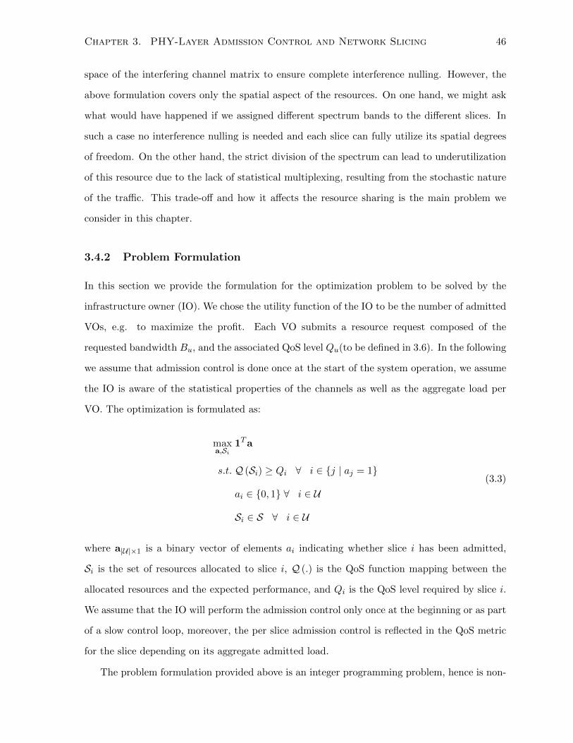
Chapter 3. PHY-Layer Admission Control and Network Slicing 46
space of the interfering channel matrix to ensure complete interference nulling. However, the
above formulation covers only the spatial aspect of the resources. On one hand, we might ask
what would have happened if we assigned different spectrum bands to the different slices. In
such a case no interference nulling is needed and each slice can fully utilize its spatial degrees
of freedom. On the other hand, the strict division of the spectrum can lead to underutilization
of this resource due to the lack of statistical multiplexing, resulting from the stochastic nature
of the traffic. This trade-off and how it affects the resource sharing is the main problem we
consider in this chapter.
3.4.2 Problem Formulation
In this section we provide the formulation for the optimization problem to be solved by the
infrastructure owner (IO). We chose the utility function of the IO to be the number of admitted
VOs, e.g. to maximize the profit. Each VO submits a resource request composed of the
requested bandwidth Bu, and the associated QoS level Qu(to be defined in 3.6). In the following
we assume that admission control is done once at the start of the system operation, we assume
the IO is aware of the statistical properties of the channels as well as the aggregate load per
VO. The optimization is formulated as:
maxa,Si
1Ta
s.t. Q (Si) ≥ Qi ∀ i ∈ {j | aj = 1}
ai ∈ {0, 1} ∀ i ∈ U
Si ∈ S ∀ i ∈ U
(3.3)
where a|U|×1 is a binary vector of elements ai indicating whether slice i has been admitted,
Si is the set of resources allocated to slice i, Q (.) is the QoS function mapping between the
allocated resources and the expected performance, and Qi is the QoS level required by slice i.
We assume that the IO will perform the admission control only once at the beginning or as part
of a slow control loop, moreover, the per slice admission control is reflected in the QoS metric
for the slice depending on its aggregate admitted load.
The problem formulation provided above is an integer programming problem, hence is non-
Chapter 3. PHY-Layer Admission Control and Network Slicing 47
convex as as well as NP-complete. In the next section, we provide the steps of our algorithm
to solve the problem as well as our definition of the QoS function.
3.5 Admission Control and Resource Slicing Algorithm
Our main problem defined in (3.3) is in general NP-hard due to its combinatoric nature. Hence,
our approach is to start with FDMA, and gradually build upon the initial slicing with SDMA
as long as the QoS criteria is satisfied. The high-level steps of the algorithm are as follows:
1. Spectrum Allocation: find a spectrum allocation such that each slice gets a spectrum
band equal to its request, while having as few conflicts between the different slices as
possible. If there is still some conflict in the allocation, i.e. some part of the spectrum is
shared between at least two slices, proceed to the admission control step.
2. Admission Control: pick a feasible set of slices such that no spectrum resource is allocated
to more than one slice.
3. Spatial Multiplexing: the final step is to greedily improve the existing set of admitted
slices by spatially multiplexing additional ones. The admission of new slices should be
such that no QoS constraint is violated.
3.5.1 Spectrum Allocation
The first step in our algorithm is to allocate a frequency band to each slice. We assume that
slices have no preference with respect to the different bands. Hence, the criteria we focus upon
is to minimize the maximum conflict, i.e. band intersection, between the different slices. This
becomes
minx
γ
s.t.γ ≥ QiQj((xi −Bi/2)− (xj +Bj/2))2 ∀ i, j ∈ U , i 6= j
γ ≥ QiQj((xi +Bi/2)− (xj −Bj/2))2 ∀ i, j ∈ U , i 6= j
xi −Bi/2 ≥ 0
− xi +Bi/2 ≤ B
(3.4)
Chapter 3. PHY-Layer Admission Control and Network Slicing 48
where xi is the center of the band allocated to slice i, and Bi is the size of the frequency
band requested by it. Note that we use the weights QiQj to penalize the intersection between
two slices with high QoS levels over lower ones. The goal of this optimization is to minimize
the maximum intersection between the allocated bands, where xi − Bi/2 is the lower end and
xi + Bi/2 is the upper end of the band allocated to slice i1. While problem (3.4) is non-
convex, we will proceed with a local optimum for it, as this is much easier to find than original
formulation in (3.3).
Note that the above problem is just about finding a spectrum allocation, possibly infeasible,
for all the possible slices. The question of feasibility, i.e. admission control, is handled next.
3.5.2 Admission Control through the Maximum Independent Set
Once the frequency bands have been decided, the next step is to pick a non-conflicting set of
slices. An example for this is shown in Fig. 3.2, where we have 7 slices with their bands already
allocated. The algorithm needs to select the best, e.g largest, non-conflicting set of slices. We
have eight independent sets of slices, {1, 2}, {3, 4, 5}, {1, 4, 5}, {6, 7}, {3, 2}, {1, 4, 7}, {3, 4, 7} and
{6, 5}, and the goal is to choose the one with the maximum weight.
In order to find a feasible solution, i.e. a set of non-intersecting frequency bands, we need
to solve:
maxa
|U|∑i=1
aiwi
s.t. ∩i:ai=1 Si = ∅ , ai ∈ {0, 1}
(3.5)
where Si is the interval {xi −Bi/2, xi +Bi/2} and xi found through solving (3.4). The first
constraint says that all admitted slices have to be non-conflicting, while the second is the binary
constraint imposed upon the decision a. This problem is essentially about selecting a subset of
non-conflicting slices of maximum weight.
The key point now is to identify that problem (3.5) is equivalent to a maximum weight
1Note that if Bi is the same for all slices, the problem becomes that of maximizing the minimum mutualdistance between all the band centers.
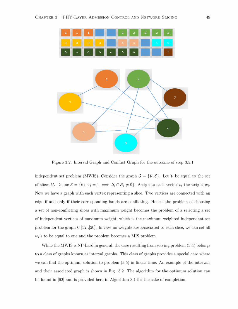
Chapter 3. PHY-Layer Admission Control and Network Slicing 49
Figure 3.2: Interval Graph and Conflict Graph for the outcome of step 3.5.1
independent set problem (MWIS). Consider the graph G = {V, E}. Let V be equal to the set
of slices U . Define E = {e : eij = 1 ⇐⇒ Si ∩ Sj 6= ∅}. Assign to each vertex vi the weight wi.
Now we have a graph with each vertex representing a slice. Two vertices are connected with an
edge if and only if their corresponding bands are conflicting. Hence, the problem of choosing
a set of non-conflicting slices with maximum weight becomes the problem of a selecting a set
of independent vertices of maximum weight, which is the maximum weighted independent set
problem for the graph G [52],[20]. In case no weights are associated to each slice, we can set all
wi’s to be equal to one and the problem becomes a MIS problem.
While the MWIS is NP-hard in general, the case resulting from solving problem (3.4) belongs
to a class of graphs known as interval graphs. This class of graphs provides a special case where
we can find the optimum solution to problem (3.5) in linear time. An example of the intervals
and their associated graph is shown in Fig. 3.2. The algorithm for the optimum solution can
be found in [62] and is provided here in Algorithm 3.1 for the sake of completion.
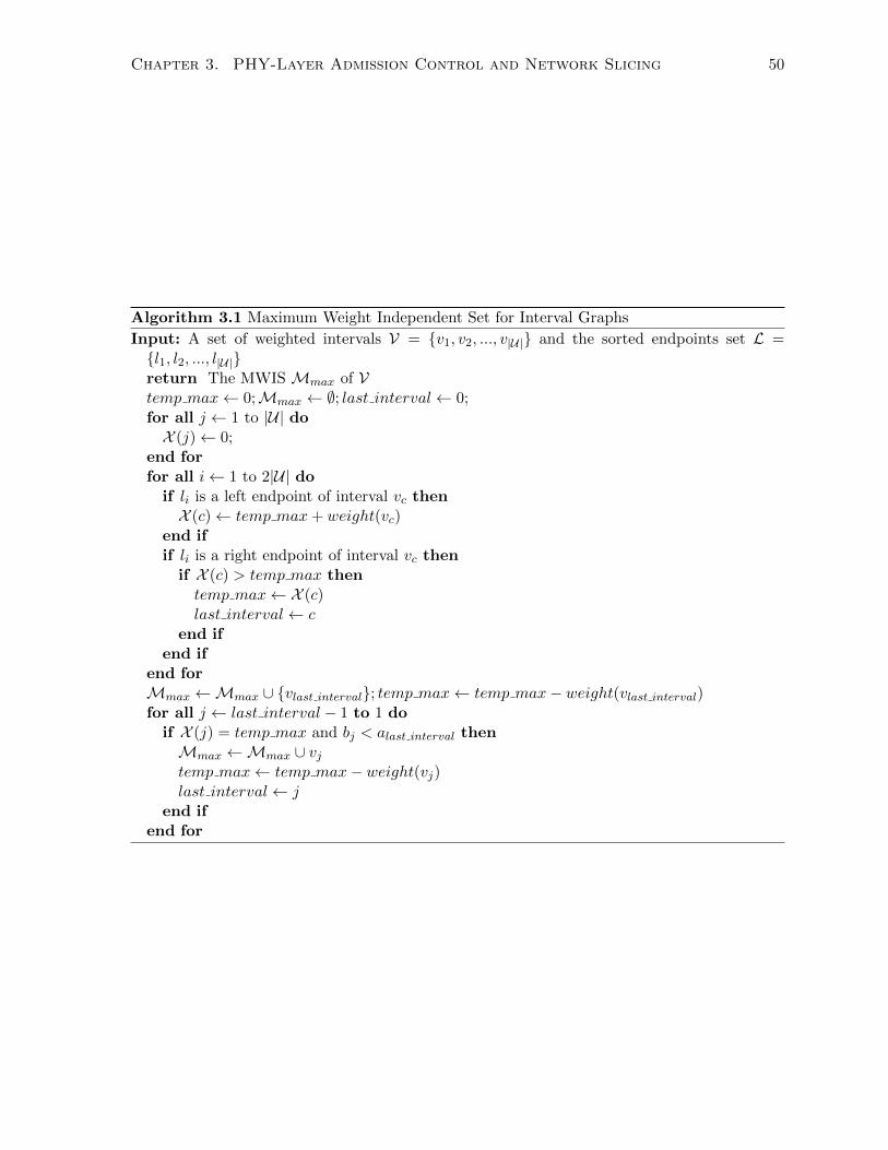
Chapter 3. PHY-Layer Admission Control and Network Slicing 50
Algorithm 3.1 Maximum Weight Independent Set for Interval Graphs
Input: A set of weighted intervals V = {v1, v2, ..., v|U|} and the sorted endpoints set L ={l1, l2, ..., l|U|}return The MWIS Mmax of Vtemp max← 0;Mmax ← ∅; last interval← 0;for all j ← 1 to |U| doX (j)← 0;
end forfor all i← 1 to 2|U| do
if li is a left endpoint of interval vc thenX (c)← temp max+ weight(vc)
end ifif li is a right endpoint of interval vc then
if X (c) > temp max thentemp max← X (c)last interval← c
end ifend if
end forMmax ←Mmax ∪ {vlast interval}; temp max← temp max− weight(vlast interval)for all j ← last interval − 1 to 1 do
if X (j) = temp max and bj < alast interval thenMmax ←Mmax ∪ vjtemp max← temp max− weight(vj)last interval← j
end ifend for
Chapter 3. PHY-Layer Admission Control and Network Slicing 51
3.5.3 SDMA
Once a feasible FDMA-based solution has been found, the final step is consider if more slices
can be spatially multiplexed with the chosen slices while still satisfying the QoS constraints.
Here, we follow a greedy approach. We consider each non-allocated slice, and examine whether
the QoS metrics are still satisfied. If this is the case, then the new slice is added and we move
on to examine the next non-allocated slice. The following section covers how we define the QoS
function.
3.6 QoS Analysis
Recall that Wu is the initial, pre-nulling, precoder designed by slice u. Without loss of general-
ity, we focus on the case where Wu = wu, i.e. one user is active at the time and the beamformer
is a vector. This is in line with the motivating example we discussed in 3.4.1.
We consider the matched filter-zero forcing precoding. In other words, each slice will match
the precoder vector to its users’ channels while projecting it into the null-upace of the other
slices’ channels. Let wu denote the precoder vector for slice u, hu is the channel for slice u and
H−u is the combined channel matrix for all the other slices. According to the matched filter
criteria, wu = h∗Tu .
In order for slice u to induce no interference on the other slices, the precoder needs to be
projected into the null space of their channel. Let us define wu = wu ⊥ Null(H−u).
We find it important now to distinguish three cases. Let k be the number of users serviced
with slices −u through the channel matrix H−u, n be the total number of antennas and m
the number of antennas allocated to slice u. In other words, the matrix H−u is of dimensions
k × n−m. These cases are:
• k > n−m
In this case of a ’tall and thin’ matrix, and assuming the matrix is of full column rank,
the null space is of dimension zero. Hence we can not find a precoder wu = wu ⊥
Null(H−u) 6= 0 and interference can not be completely removed using spatial beamform-
ing.
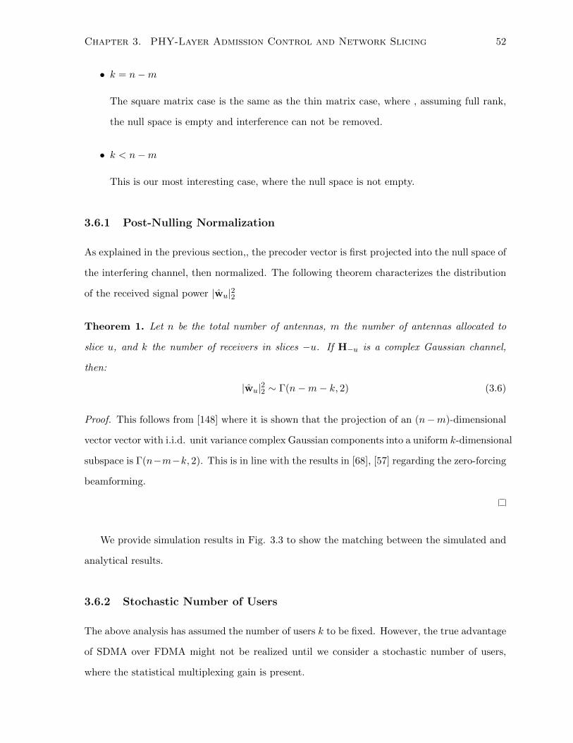
Chapter 3. PHY-Layer Admission Control and Network Slicing 52
• k = n−m
The square matrix case is the same as the thin matrix case, where , assuming full rank,
the null space is empty and interference can not be removed.
• k < n−m
This is our most interesting case, where the null space is not empty.
3.6.1 Post-Nulling Normalization
As explained in the previous section,, the precoder vector is first projected into the null space of
the interfering channel, then normalized. The following theorem characterizes the distribution
of the received signal power |wu|22
Theorem 1. Let n be the total number of antennas, m the number of antennas allocated to
slice u, and k the number of receivers in slices −u. If H−u is a complex Gaussian channel,
then:
|wu|22 ∼ Γ(n−m− k, 2) (3.6)
Proof. This follows from [148] where it is shown that the projection of an (n−m)-dimensional
vector vector with i.i.d. unit variance complex Gaussian components into a uniform k-dimensional
subspace is Γ(n−m−k, 2). This is in line with the results in [68], [57] regarding the zero-forcing
beamforming.
We provide simulation results in Fig. 3.3 to show the matching between the simulated and
analytical results.
3.6.2 Stochastic Number of Users
The above analysis has assumed the number of users k to be fixed. However, the true advantage
of SDMA over FDMA might not be realized until we consider a stochastic number of users,
where the statistical multiplexing gain is present.
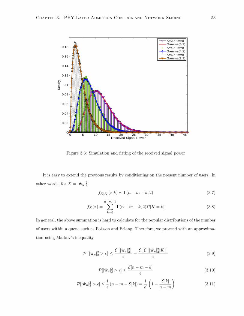
Chapter 3. PHY-Layer Admission Control and Network Slicing 53
0 5 10 15 20 25 30 35 40 450
0.02
0.04
0.06
0.08
0.1
0.12
0.14
0.16
0.18
Received Signal Power
Den
sity
K=2,n−m=8Gamma(6,2)K=4,n−m=8Gamma(4,2)K=6,n−m=8Gamma(2,2)
Figure 3.3: Simulation and fitting of the received signal power
It is easy to extend the previous results by conditioning on the present number of users. In
other words, for X = |wu|22
fX|K (x|k) ∼ Γ(n−m− k, 2) (3.7)
fX(x) =n−m−1∑k=0
Γ(n−m− k, 2)P[K = k] (3.8)
In general, the above summation is hard to calculate for the popular distributions of the number
of users within a queue such as Poisson and Erlang. Therefore, we proceed with an approxima-
tion using Markov’s inequality
P[|wu|22 > ε
]≤E[|wu|22
]ε
=E[E[|wu|22|K
]]ε
(3.9)
P[|wu|22 > ε] ≤ E [n−m− k]
ε(3.10)
P[|wu|22 > ε] ≤ 1
ε(n−m− E [k]) =
1
ε′
(1− E [k]
n−m
)(3.11)
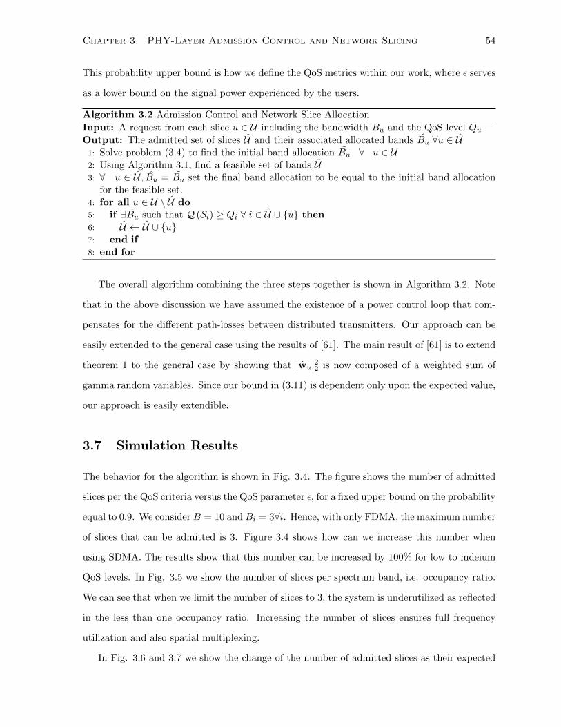
Chapter 3. PHY-Layer Admission Control and Network Slicing 54
This probability upper bound is how we define the QoS metrics within our work, where ε serves
as a lower bound on the signal power experienced by the users.
Algorithm 3.2 Admission Control and Network Slice Allocation
Input: A request from each slice u ∈ U including the bandwidth Bu and the QoS level QuOutput: The admitted set of slices U and their associated allocated bands Bu ∀u ∈ U
1: Solve problem (3.4) to find the initial band allocation Bu ∀ u ∈ U2: Using Algorithm 3.1, find a feasible set of bands U3: ∀ u ∈ U , Bu = Bu set the final band allocation to be equal to the initial band allocation
for the feasible set.4: for all u ∈ U \ U do5: if ∃Bu such that Q (Si) ≥ Qi ∀ i ∈ U ∪ {u} then6: U ← U ∪ {u}7: end if8: end for
The overall algorithm combining the three steps together is shown in Algorithm 3.2. Note
that in the above discussion we have assumed the existence of a power control loop that com-
pensates for the different path-losses between distributed transmitters. Our approach can be
easily extended to the general case using the results of [61]. The main result of [61] is to extend
theorem 1 to the general case by showing that |wu|22 is now composed of a weighted sum of
gamma random variables. Since our bound in (3.11) is dependent only upon the expected value,
our approach is easily extendible.
3.7 Simulation Results
The behavior for the algorithm is shown in Fig. 3.4. The figure shows the number of admitted
slices per the QoS criteria versus the QoS parameter ε, for a fixed upper bound on the probability
equal to 0.9. We consider B = 10 and Bi = 3∀i. Hence, with only FDMA, the maximum number
of slices that can be admitted is 3. Figure 3.4 shows how can we increase this number when
using SDMA. The results show that this number can be increased by 100% for low to mdeium
QoS levels. In Fig. 3.5 we show the number of slices per spectrum band, i.e. occupancy ratio.
We can see that when we limit the number of slices to 3, the system is underutilized as reflected
in the less than one occupancy ratio. Increasing the number of slices ensures full frequency
utilization and also spatial multiplexing.
In Fig. 3.6 and 3.7 we show the change of the number of admitted slices as their expected
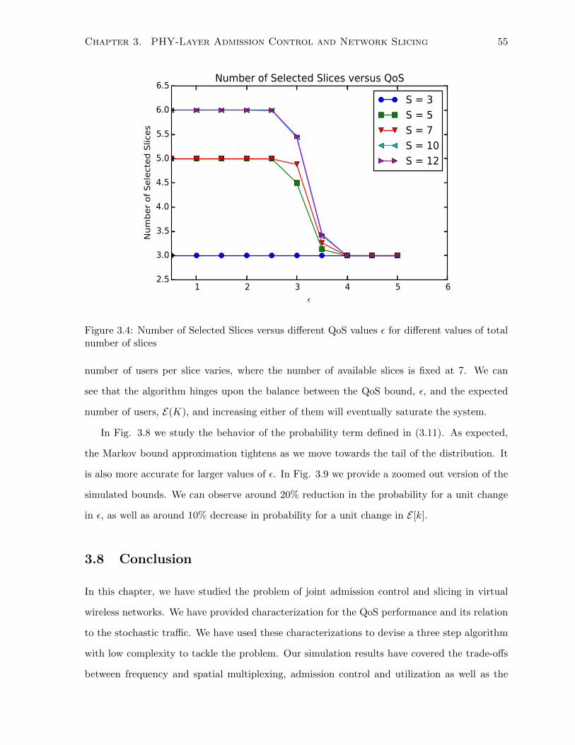
Chapter 3. PHY-Layer Admission Control and Network Slicing 55
1 2 3 4 5 6ε
2.5
3.0
3.5
4.0
4.5
5.0
5.5
6.0
6.5
Number of Selected Slice
s
Number of Selected Slices versus QoS
S = 3
S = 5
S = 7
S = 10
S = 12
Figure 3.4: Number of Selected Slices versus different QoS values ε for different values of totalnumber of slices
number of users per slice varies, where the number of available slices is fixed at 7. We can
see that the algorithm hinges upon the balance between the QoS bound, ε, and the expected
number of users, E(K), and increasing either of them will eventually saturate the system.
In Fig. 3.8 we study the behavior of the probability term defined in (3.11). As expected,
the Markov bound approximation tightens as we move towards the tail of the distribution. It
is also more accurate for larger values of ε. In Fig. 3.9 we provide a zoomed out version of the
simulated bounds. We can observe around 20% reduction in the probability for a unit change
in ε, as well as around 10% decrease in probability for a unit change in E [k].
3.8 Conclusion
In this chapter, we have studied the problem of joint admission control and slicing in virtual
wireless networks. We have provided characterization for the QoS performance and its relation
to the stochastic traffic. We have used these characterizations to devise a three step algorithm
with low complexity to tackle the problem. Our simulation results have covered the trade-offs
between frequency and spatial multiplexing, admission control and utilization as well as the
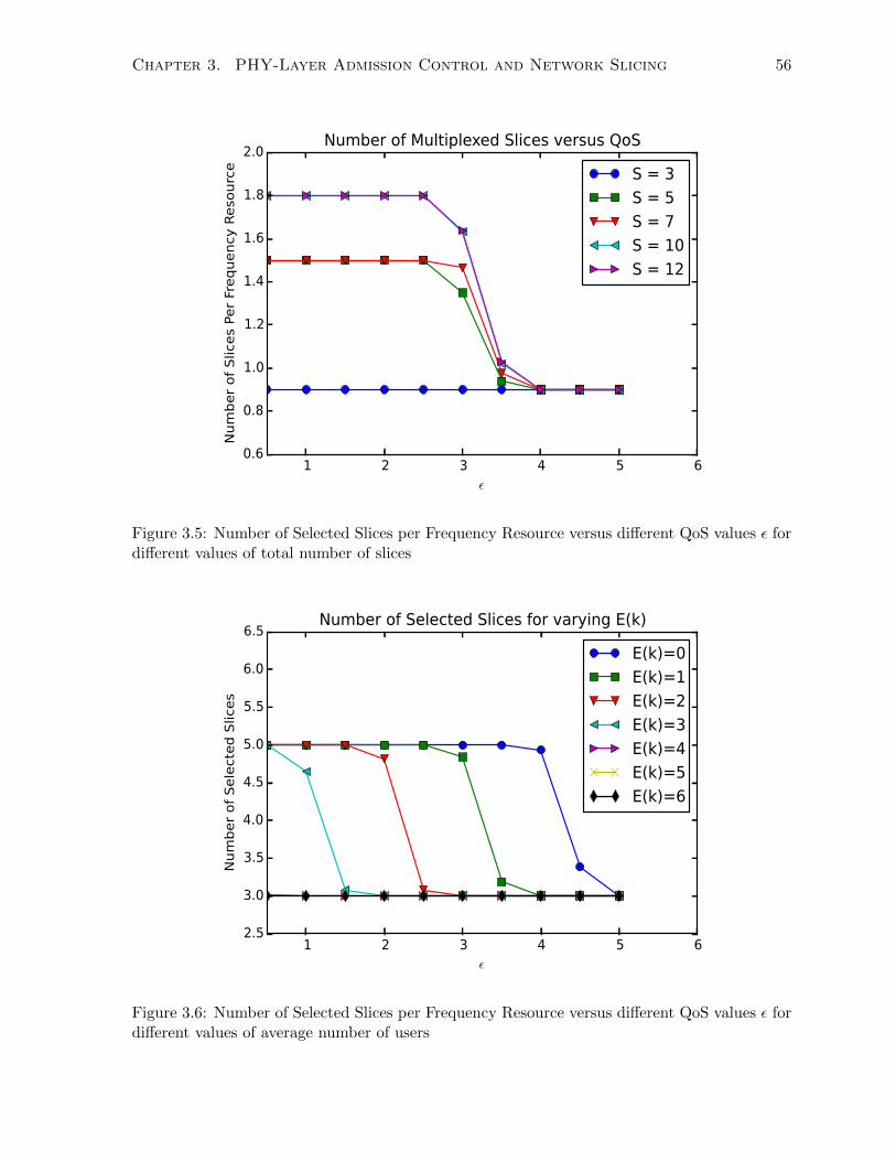
Chapter 3. PHY-Layer Admission Control and Network Slicing 56
1 2 3 4 5 6ε
0.6
0.8
1.0
1.2
1.4
1.6
1.8
2.0
Number of Slice
s Per Frequency
Reso
urce
Number of Multiplexed Slices versus QoS
S = 3
S = 5
S = 7
S = 10
S = 12
Figure 3.5: Number of Selected Slices per Frequency Resource versus different QoS values ε fordifferent values of total number of slices
1 2 3 4 5 6ε
2.5
3.0
3.5
4.0
4.5
5.0
5.5
6.0
6.5
Number of Selected Slices
Number of Selected Slices for varying E(k)
E(k)=0
E(k)=1
E(k)=2
E(k)=3
E(k)=4
E(k)=5
E(k)=6
Figure 3.6: Number of Selected Slices per Frequency Resource versus different QoS values ε fordifferent values of average number of users
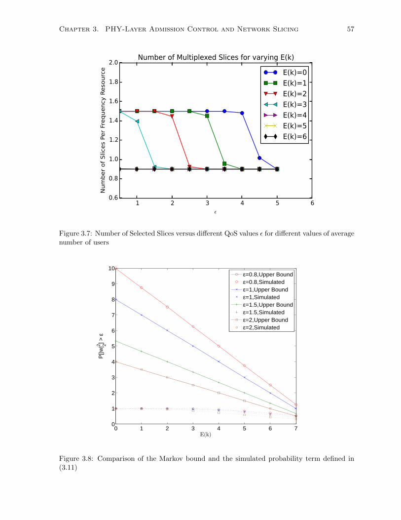
Chapter 3. PHY-Layer Admission Control and Network Slicing 57
1 2 3 4 5 6ε
0.6
0.8
1.0
1.2
1.4
1.6
1.8
2.0
Number of Slices Per Frequency Resource
Number of Multiplexed Slices for varying E(k)
E(k)=0
E(k)=1
E(k)=2
E(k)=3
E(k)=4
E(k)=5
E(k)=6
Figure 3.7: Number of Selected Slices versus different QoS values ε for different values of averagenumber of users
0 1 2 3 4 5 6 70
1
2
3
4
5
6
7
8
9
10
E(k)
P[|w
|2 2] > ε
ε=0.8,Upper Boundε=0.8,Simulatedε=1,Upper Boundε=1,Simulatedε=1.5,Upper Boundε=1.5,Simulatedε=2,Upper Boundε=2,Simulated
Figure 3.8: Comparison of the Markov bound and the simulated probability term defined in(3.11)
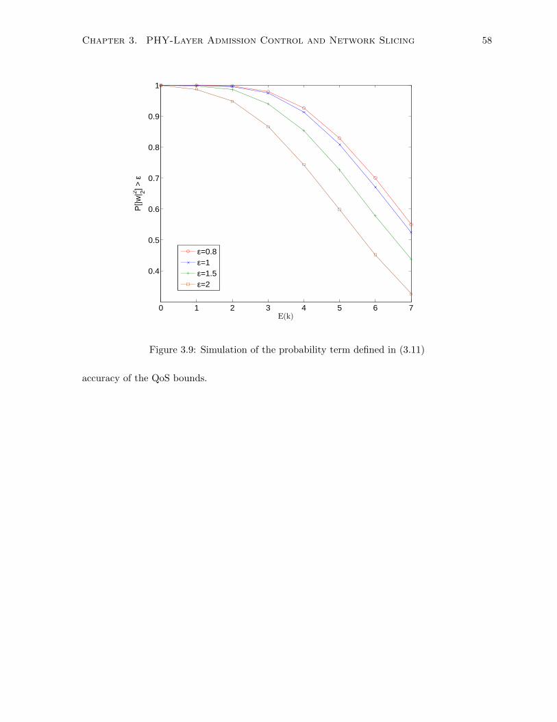
Chapter 3. PHY-Layer Admission Control and Network Slicing 58
0 1 2 3 4 5 6 7
0.4
0.5
0.6
0.7
0.8
0.9
1
E(k)
P[|w
|2 2] > ε
ε=0.8ε=1ε=1.5ε=2
Figure 3.9: Simulation of the probability term defined in (3.11)
accuracy of the QoS bounds.
Chapter 4
Multi-Operator Scheduling in
Cloud-RANs
4.1 Context
The software-defined approach of cloud radio access networks (C-RANs) enables supporting
multiple virtual operators (VOs) on the same physical infrastructure. In this shared envi-
ronment, a coordinator is needed to manage the sharing of resources between the VOs. In
Chapter 3 we studied how this coordination can be achieved through null-space projection. In
this chapter, we look at another form coordination, that is hierarchal scheduling. Designing
a scheduling coordinator is about striking a good balance between the flexibility given to the
VOs, and the efficiency of the resource utilization. In particular, we study the problem of coor-
dinated scheduling in the multi-operator cloud-RAN environment. We formulate the problem
as a two-stage scheduling, where in the first stage the VOs are responsible for scheduling their
own users, after which they submit their resource requests to a centralized coordinator. The
coordinator selects a subset of non-conflicting requests for transmission. We show that the
problem in the general case is NP-hard. We then discuss two special cases and relate them
to the existing communication protocols. By gaining insights from these two special cases, we
propose a general heuristic, which works on any formulation of the problem, and is still able
to provide close-to-optimum performance in the special cases we considered. The heuristic is
59
Chapter 4. Multi-Operator Scheduling in Cloud-RANs 60
shown to have some similarities to the neuro-computation techniques such as Hopfield-network.
Finally, simulation results are provided to show the efficiency of the proposed algorithms.
4.2 Introduction
The concept of cloud-RANs is closely related to that of software-defined networking (SDN)[75]
and network virtualization[32]. Overall, one of the main goals of these technologies is to be
able to support distributed computing capabilities, in the form of data-center servers, as well
as share the physical infrastructure between different network operators. A challenge unique to
wireless networks is sharing the air interface between the VOs. In such a case, designing efficient
coordination schemes between these VOs is tricky. On one hand, SDN and virtual network-
ing advocate the diversity of services and technologies to be supported by the different VOs.
Hence, VOs need to have sufficient control over the resources given to them in order to provide
service-differentiation for their customers. On the other hand, in such highly-heterogeneous
environment, coming up with efficient coordination decisions is hard. The question remains
open about how to coordinate VOs with heterogeneous MAC-layers or even PHY-layers.
In Chapter 3 we studied how interference coordination through null space projection can
be used to share the resources between the different slices. In this chapter we study another
form of interference coordination through hierarchal scheduling. This is a form of scheduling
where the decision is made in two stages; first each slice selects a subset of its own users, then
the infrastructure controller selects which slices get access to the spectrum resources within the
next time slot. However, the challenge here is how to balance the flexibility given to the slices
with the overall system utilization. In other words, in order for the infrastructure controller to
truly optimize the system utilization, it needs to do a more detailed scheduling. This, however,
would lead to less flexibility given to the slice controller.
The cloud-RAN architecture is expected to host a diverse set of network slices, each with
its own PHY and MAC technologies. The reason for this, as discussed in Chapter 3, is that
different applications impose different requirements on the PHY and MAC layers. For example,
sensor networks need low power transmission, while augmented reality applications need low
latency. Sensor networks might use spread spectrum techniques while augmented reality might
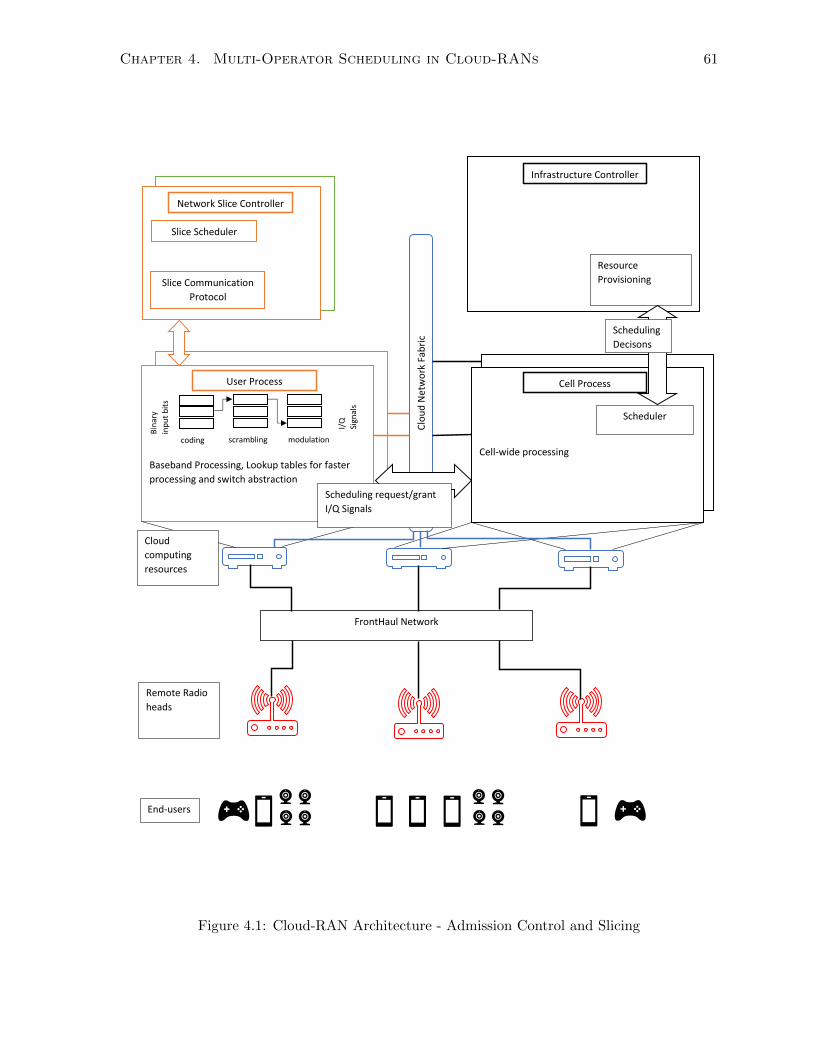
Chapter 4. Multi-Operator Scheduling in Cloud-RANs 61
Baseband Processing, Lookup tables for faster
processing and switch abstraction
Baseband Processing, Lookup tables for faster
processing and switch abstraction
Baseband Processing, Lookup tables for faster
processing and switch abstraction
FrontHaul Network
coding scrambling modulation
Bin
ary
inp
ut
bit
s
I/Q
Sign
als
Cloud
computing
resources
Remote Radio
heads
Cell-wide processing
User Process Cell Process
Scheduler
Network Slice Controller
Slice Scheduler
Slice Communication
Protocol
Infrastructure Controller
Resource
Provisioning
Clo
ud
Net
wo
rk F
abri
c
Scheduling
Decisons
Scheduling request/grant
I/Q Signals
End-users
Figure 4.1: Cloud-RAN Architecture - Admission Control and Slicing
Chapter 4. Multi-Operator Scheduling in Cloud-RANs 62
use time division techniques. Different PHY technologies have different ways to allocate the
spectrum resources. For example, in LTE and other OFDMA systems, part of the spectrum
is used as a control channel to notify each user which resources, if any, it has been assigned.
Hence, resource assignment is a complicated process that needs access to multiple resources
simultaneously, i.e. an LTE slice needs access to both the control and data resource blocks to
correctly deliver data in order to its user.
For the reasons discussed in the above discussions, we decided to limit the infrastructure
controller decision to be a Yes/No one. Each slice will select which set of resources it needs to
access within the next time slot, including all the data and control ones. Then the infrastructure
controller decides whether the slice gets to use all these requested resources or none at all. This
ensures that the slice can choose its own arbitrary data/control resource splitting scheme, and
the infrastructure controller decision is agnostic to how this choice or design is made.
In Fig. 4.1 we show the system architecture focusing on the multi-slice scheduling parts.
In particular, we study the trade-off between the flexibility given to VOs, and the efficiency
of the coordinator decisions. We consider a scenario where the VOs have their computing
resources in the data center. These computing resources prepare a resource request. This
request includes the specification of the requested resource, e.g. frequency band or resource
block, the modulation and coding scheme (MCS) to be used and so on. By allowing the VOs
to choose the resources and their MCS, they are given sufficient control to provide the desired
service differentiation for their users. These resource requests are then received at a central
coordinator. In order to be able to accommodate requests from heterogeneous VOs, the decision
of the coordinator is constrained to a Yes/No decision. In other words, the coordinator chooses
only a subset of the requests without altering them. We show that the problem is equivalent
to a maximum weighted independent set problem (MWIS), a well-known problem in Graph
theory and complexity theory [52]. Maximum independent set problems are both NP-hard[52]
and APX-hard [20], i.e. they are as hard to approximate as to solve. Next, we discuss two
special cases, where the resources being requested have to form a contiguous set, similar to the
constraint in the LTE uplink. We provide the optimum algorithms for these cases, for which
the complexity is either logarithmic or linear. Finally, we propose an efficient heuristic, which
is able to work on the general problem, and can provide very-efficient solutions for the special
Chapter 4. Multi-Operator Scheduling in Cloud-RANs 63
cases discussed.
4.3 Related Work
The literature on scheduling for for wireless virtualization is growing rapidly. The NVS archi-
tecture proposed in [114] discussed two-level scheduling for WiMAX systems. In this case, all
the network slices are limited to use WiMAX, and while the same architecture can be applied to
other OFDMA systems such as LTE, the limitation on the homogeneity of the slices still stands.
In the LTE architecture proposed in [160] the infrastructure controller, called Hypervisor, has
direct access to the slice schedulers. In other words, the Hypervisor handles all the scheduling
and slices have no direct control over how their own users are scheduled. A stochastic game
framework was proposed in [46] based on the VCG mechanism. This is a utility maximization
where the slices are competing for the resources, but may get only a subset of the resources
they request. This is not our goal as we have explained before the strong coupling between data
and control resources needed for successful service. Opportunistic scheduling was proposed for
WiFi systems in [154] where different slices can be scheduled on the same channel subject to
a limit on the collision probability. However, no work has considered the case when both LTE
and WiFi are present in the network.
In summary, most of the existing works have focused on OFDM-based scheduling. However,
this assumption may not necessarily hold in future networks. For example, IEEE802.15.4 has
already standardized the use of spread spectrum for wireless sensor networks due to its superior
performance in low power scenarios. Moreover, those works have not considered the coupling
between the requested resources and the fact that if the slice is not assigned all the requested
resources, it might not be able to utilize any of them. Another drawback of the existing work
is the centralized nature of the processing, where the baseband processing and scheduling are
performed within the same physical machine, typically a base-station FPGA. In other words, the
challenges associated with cloud-RANs are not discussed. Finally, extending these techniques
to Coordinated multi-point (CoMP)[50] scenarios is not straight-forward, as they are mainly
designed for the single transmitter case.
Chapter 4. Multi-Operator Scheduling in Cloud-RANs 64
4.4 System Model
Consider a cloud-RAN system where a cloud data center forwards the I/Q signals through a
high-speed network to a set of RRHs. Let S be the set of resources, which may include frequency,
time, space or code resources. Let U be the set of VOs, also referred to as network slices. Each
VO i ∈ U prepares a request specifying the desired subset of resources. Let Si denote such a
request. Each request Si comes associated with a weight wi. This weight, as well as the size
of the request, is used by the coordinator to compare between the different requests. Different
scheduling weights have been discussed in the literature, see [42] for a survey. The scheduling
decisions discussed here are to replace the scheduling decisions in the current architectures,
hence will occur with the same frequency as them.
In this chapter we are not concerned with the design of the scheduling weights, rather that
the VOs and the coordinator agree on a specific weighting criteria. The decision made by the
coordinator is as follows:
Problem 4.1:
maxx
|U|∑i=1
xiwi
s.t. ∩i:xi=1 Si = ∅
xi ∈ {0, 1}
(4.1)
where x is the decision made by the coordinator, xi = 1 means that the request Si has been
accepted, and zero otherwise. The first constraint says that all accepted requests have to be
non-conflicting, while the second is the binary constraint imposed upon the decision x. This
problem is about selecting a subset of non-conflicting requests of maximum weight.
Theorem 2. Problem 4.1 is NP-hard. Moreover, the problem is APX-hard.
Proof. The proof follows by showing that the problem is equivalent to a maximum weighted
independent set problem. Consider the graph G = {V, E}. Let V be equal to the set of VOs
U . Define E = {e : eij = 1 ⇐⇒ Si ∩ Sj 6= ∅}. Assign to each vertex vi the weight wi. Now we
have a graph with each vertex representing a request. Two vertices are connected with an edge
if and only if their corresponding requests are conflicting. Hence, the problem of choosing a
Chapter 4. Multi-Operator Scheduling in Cloud-RANs 65
set of non-conflicting requests with maximum weight becomes the problem of a selecting a set
of non-connected vertices of maximum weight, which is the maximum weighted independent
set problem for the graph G. From the properties of MWIS problem [52],[20], the theorem
follows.
4.5 Scheduling Algorithms for VOs
In this section, we discuss two special cases for Problem (4.1) which have polynomial time
optimum solutions. Then we discuss how these two algorithms can be extended to solve problem
(4.1) in its general form.
4.5.1 Case 1
Due to the difficulty of problem (4.1), we discuss now how it can be efficiently solved in a special
case. Let I ={
20, 21, ..., 2i, 2i+1, ..., 2log2(|S|)}
, where |S| is assumed to be a power of two. We
impose the following set of conditions upon any request:
1. |Si| ∈ I.
2. Let s0, ..., sN−1 be the elements of S. Let Si = {sk, sk+1, ..., sm}. Then k mod 2 =
0 ∀ k 6= m.
The first condition says that the size of any request has to be a power of 2. The intuition
behind the second constraint is that these requests represent nodes of a binary tree.
The algorithm for solving the case 1 problem is composed of three steps:
Building the Tree
The tree is constructed as follows:
(a) The tree is of height log2(|S|), and the number of leaf nodes is |S|.
(b) The tree is composed of a set of nodes tl,j , where 0 ≤ l ≤ log2(|S|) is the index of the
current level of the tree and 0 ≤ j ≤ 2l − 1 is the index of the node within level l.
(c) For each leaf node tlog2(|S|),j , associate the resource Stlog2(|S|),j = {sj}.
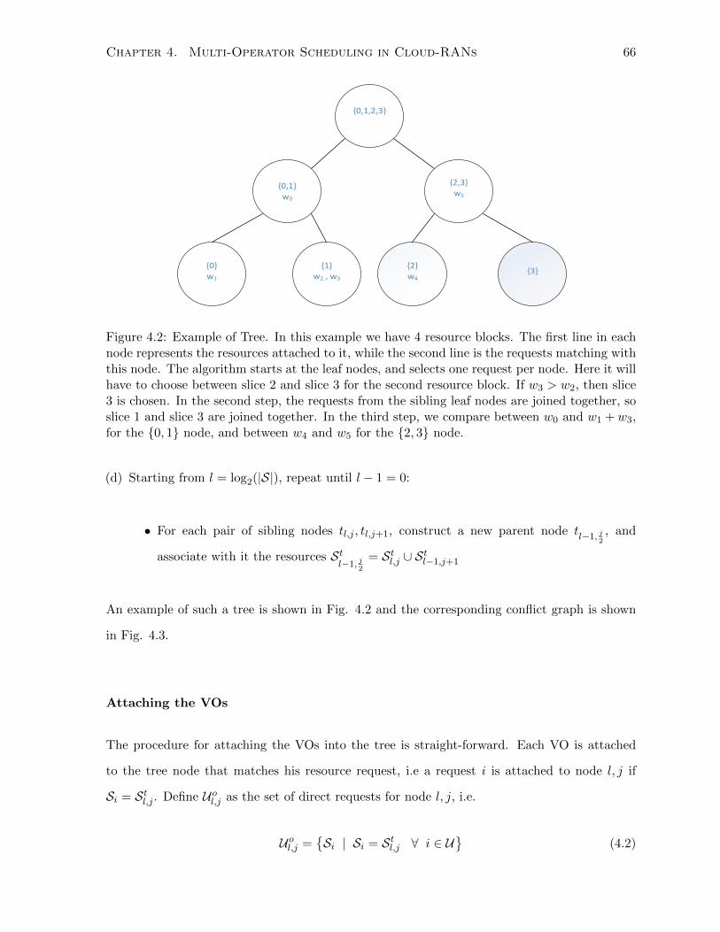
Chapter 4. Multi-Operator Scheduling in Cloud-RANs 66
{0,1,2,3}
{0,1}w0
{2,3}w5
{0}w1
{1}w2 , w3
{2}w4
{3}
Figure 4.2: Example of Tree. In this example we have 4 resource blocks. The first line in eachnode represents the resources attached to it, while the second line is the requests matching withthis node. The algorithm starts at the leaf nodes, and selects one request per node. Here it willhave to choose between slice 2 and slice 3 for the second resource block. If w3 > w2, then slice3 is chosen. In the second step, the requests from the sibling leaf nodes are joined together, soslice 1 and slice 3 are joined together. In the third step, we compare between w0 and w1 +w3,for the {0, 1} node, and between w4 and w5 for the {2, 3} node.
(d) Starting from l = log2(|S|), repeat until l − 1 = 0:
• For each pair of sibling nodes tl,j , tl,j+1, construct a new parent node tl−1, j2, and
associate with it the resources Stl−1, j
2
= Stl,j ∪ Stl−1,j+1
An example of such a tree is shown in Fig. 4.2 and the corresponding conflict graph is shown
in Fig. 4.3.
Attaching the VOs
The procedure for attaching the VOs into the tree is straight-forward. Each VO is attached
to the tree node that matches his resource request, i.e a request i is attached to node l, j if
Si = Stl,j . Define Uol,j as the set of direct requests for node l, j, i.e.
Uol,j ={Si | Si = Stl,j ∀ i ∈ U
}(4.2)
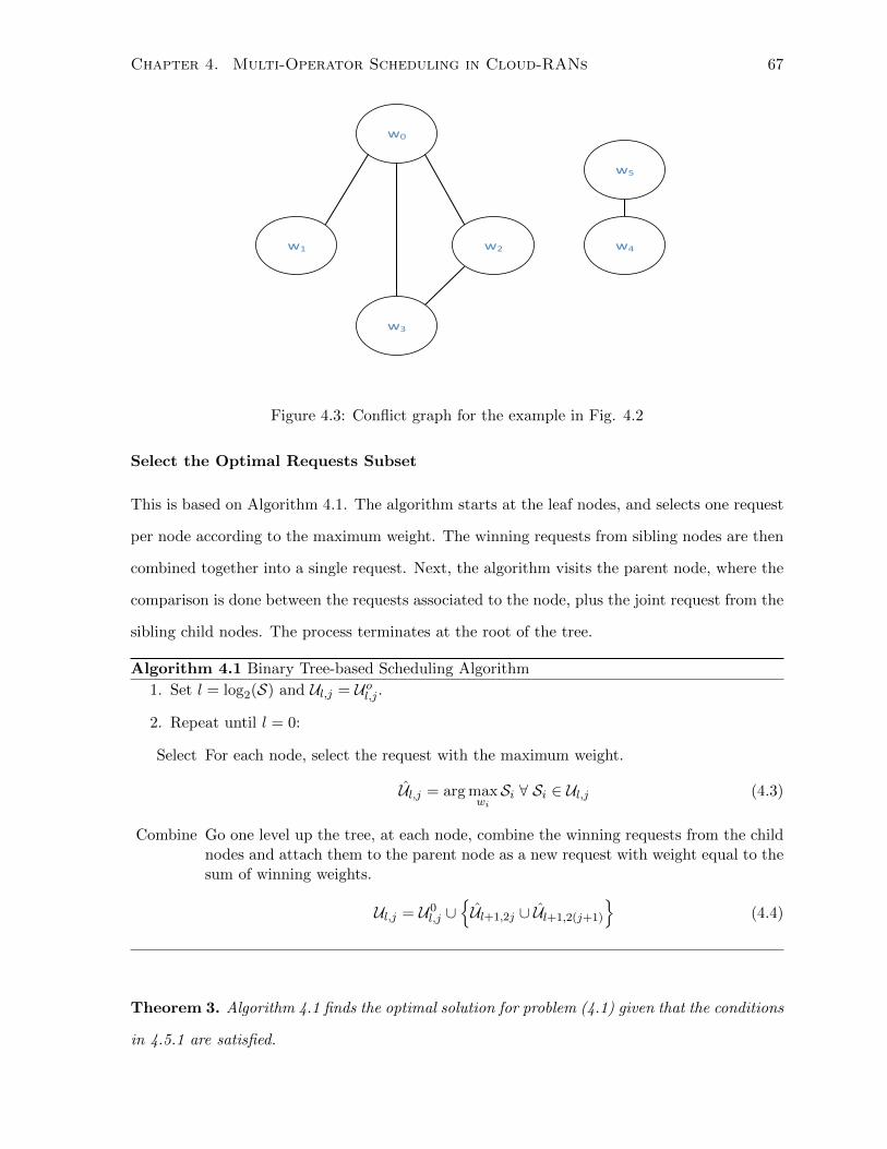
Chapter 4. Multi-Operator Scheduling in Cloud-RANs 67
w0
w1
w3
w2
w5
w4
Figure 4.3: Conflict graph for the example in Fig. 4.2
Select the Optimal Requests Subset
This is based on Algorithm 4.1. The algorithm starts at the leaf nodes, and selects one request
per node according to the maximum weight. The winning requests from sibling nodes are then
combined together into a single request. Next, the algorithm visits the parent node, where the
comparison is done between the requests associated to the node, plus the joint request from the
sibling child nodes. The process terminates at the root of the tree.
Algorithm 4.1 Binary Tree-based Scheduling Algorithm
1. Set l = log2(S) and Ul,j = Uol,j .
2. Repeat until l = 0:
Select For each node, select the request with the maximum weight.
Ul,j = arg maxwiSi ∀ Si ∈ Ul,j (4.3)
Combine Go one level up the tree, at each node, combine the winning requests from the childnodes and attach them to the parent node as a new request with weight equal to thesum of winning weights.
Ul,j = U0l,j ∪
{Ul+1,2j ∪ Ul+1,2(j+1)
}(4.4)
Theorem 3. Algorithm 4.1 finds the optimal solution for problem (4.1) given that the conditions
in 4.5.1 are satisfied.
Chapter 4. Multi-Operator Scheduling in Cloud-RANs 68
Proof. Let C∗ be the selected subset of resource requests output from Algorithm 4.1 with overall
weight w∗. Suppose another subset C is to have an overall weight w > w∗. Without loss of
generality, suppose C = C∗ − Sk + Sl. We consider two cases:
1. |Sk| = |Sl| : in this case a tree node has chosen Sk instead of Sl. Hence, w = w∗ −wk +
wl. However, from the definition of the select step in Algorithm 4.1, wk > wl, hence,
−wk + wl > 0 and w∗ > w, i.e. a contradiction.
2. Sk ⊂ Sl : in this case, the rejection of Sk happened at one of its parent nodes. However,
from the definition of both the select and combine steps in Algorithm 4.1, either w > w∗
leads to a contradiction or C is an infeasible solution.
Since the number of steps of the algorithm is equal to the depth of the tree, the complexity of
the algorithm is O(log2(|S|)).
4.5.2 Case 2
The logarithmic complexity of the above algorithm makes it an attractive way to address the
difficulty of problem 1. However, the constraints imposed upon the resource requests may
result in degradation of performance compared to the general case, or may be too tight for
some applications. In this part, we discuss another special case, which is also shown to have a
polynomial time optimal solution with less constraints than the previous case. In our current
case, the only constraint we require is:
• Si is contiguous for all i ∈ U .
Such class of graphs where the vertices can be mapped into a set of intervals on the real line is
known as Interval Graphs. An example of such class of graphs is shown in Fig. 4.4. The MWIS
problem for interval graphs has been studied in [62], where an optimal algorithm of O(|S|) was
proposed. This is the same algorithm we have discussed in 3.1.
4.5.3 Applications of Case 1 and 2
The main condition imposed upon the scheduling request in both case 1 and 2 is that the
requested resources have to be contiguous. This condition is already present in the LTE uplink,
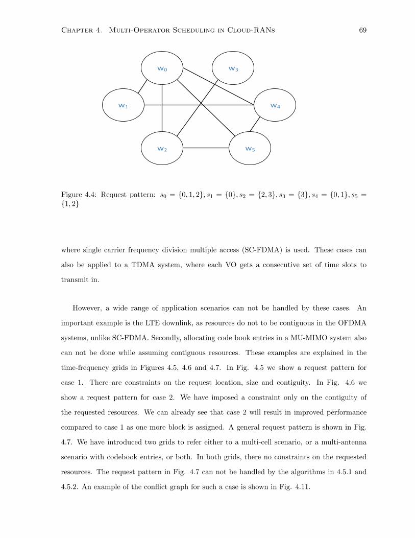
Chapter 4. Multi-Operator Scheduling in Cloud-RANs 69
w0
w1
w2
w3
w4
w5
Figure 4.4: Request pattern: s0 = {0, 1, 2}, s1 = {0}, s2 = {2, 3}, s3 = {3}, s4 = {0, 1}, s5 ={1, 2}
where single carrier frequency division multiple access (SC-FDMA) is used. These cases can
also be applied to a TDMA system, where each VO gets a consecutive set of time slots to
transmit in.
However, a wide range of application scenarios can not be handled by these cases. An
important example is the LTE downlink, as resources do not to be contiguous in the OFDMA
systems, unlike SC-FDMA. Secondly, allocating code book entries in a MU-MIMO system also
can not be done while assuming contiguous resources. These examples are explained in the
time-frequency grids in Figures 4.5, 4.6 and 4.7. In Fig. 4.5 we show a request pattern for
case 1. There are constraints on the request location, size and contiguity. In Fig. 4.6 we
show a request pattern for case 2. We have imposed a constraint only on the contiguity of
the requested resources. We can already see that case 2 will result in improved performance
compared to case 1 as one more block is assigned. A general request pattern is shown in Fig.
4.7. We have introduced two grids to refer either to a multi-cell scenario, or a multi-antenna
scenario with codebook entries, or both. In both grids, there no constraints on the requested
resources. The request pattern in Fig. 4.7 can not be handled by the algorithms in 4.5.1 and
4.5.2. An example of the conflict graph for such a case is shown in Fig. 4.11.
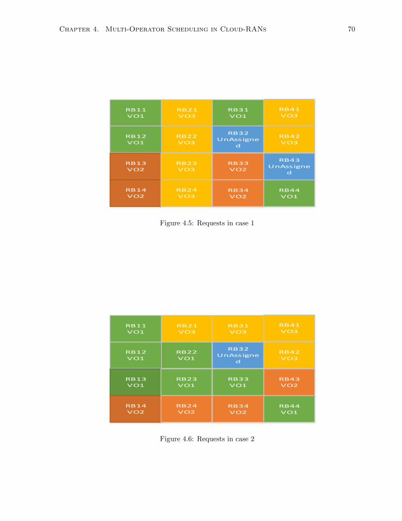
Chapter 4. Multi-Operator Scheduling in Cloud-RANs 70
RB11VO1
RB21VO3
RB22VO3
RB12VO1
RB31VO1
RB32UnAssigne
d
RB13VO2
RB23VO3
RB33VO2
RB14VO2
RB24VO3
RB34VO2
RB44VO1
RB43UnAssigne
d
RB42VO3
RB41VO3
Figure 4.5: Requests in case 1
RB11VO1
RB21VO3
RB22VO1
RB12VO1
RB31VO3
RB32UnAssigne
d
RB13VO1
RB23VO1
RB33VO1
RB14VO2
RB24VO2
RB34VO2
RB44VO1
RB43VO2
RB42VO3
RB41VO3
Figure 4.6: Requests in case 2
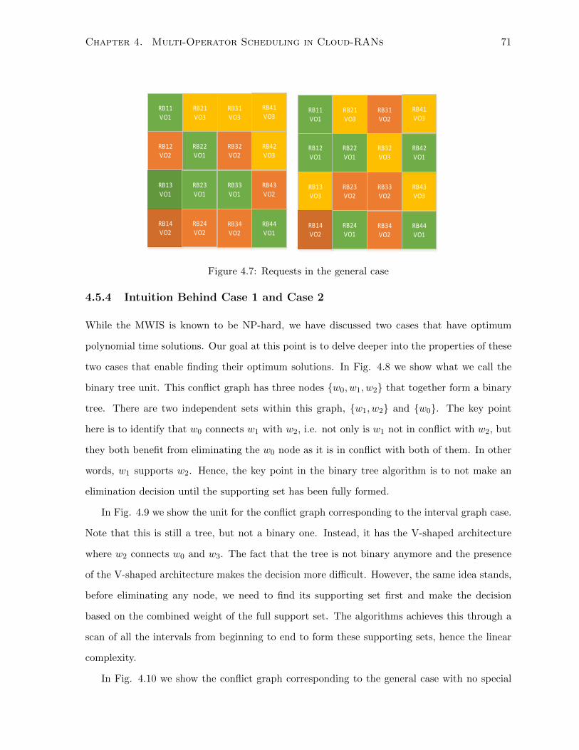
Chapter 4. Multi-Operator Scheduling in Cloud-RANs 71
RB11VO1
RB21VO3
RB22VO1
RB12VO2
RB31VO3
RB32VO2
RB13VO1
RB23VO1
RB33VO1
RB14VO2
RB24VO2
RB34VO2
RB44VO1
RB43VO2
RB42VO3
RB41VO3
RB11VO1
RB21VO3
RB22VO1
RB12VO1
RB31VO2
RB32VO3
RB13VO3
RB23VO2
RB33VO2
RB14VO2
RB24VO1
RB34VO2
RB44VO1
RB43VO3
RB42VO1
RB41VO3
Figure 4.7: Requests in the general case
4.5.4 Intuition Behind Case 1 and Case 2
While the MWIS is known to be NP-hard, we have discussed two cases that have optimum
polynomial time solutions. Our goal at this point is to delve deeper into the properties of these
two cases that enable finding their optimum solutions. In Fig. 4.8 we show what we call the
binary tree unit. This conflict graph has three nodes {w0, w1, w2} that together form a binary
tree. There are two independent sets within this graph, {w1, w2} and {w0}. The key point
here is to identify that w0 connects w1 with w2, i.e. not only is w1 not in conflict with w2, but
they both benefit from eliminating the w0 node as it is in conflict with both of them. In other
words, w1 supports w2. Hence, the key point in the binary tree algorithm is to not make an
elimination decision until the supporting set has been fully formed.
In Fig. 4.9 we show the unit for the conflict graph corresponding to the interval graph case.
Note that this is still a tree, but not a binary one. Instead, it has the V-shaped architecture
where w2 connects w0 and w3. The fact that the tree is not binary anymore and the presence
of the V-shaped architecture makes the decision more difficult. However, the same idea stands,
before eliminating any node, we need to find its supporting set first and make the decision
based on the combined weight of the full support set. The algorithms achieves this through a
scan of all the intervals from beginning to end to form these supporting sets, hence the linear
complexity.
In Fig. 4.10 we show the conflict graph corresponding to the general case with no special
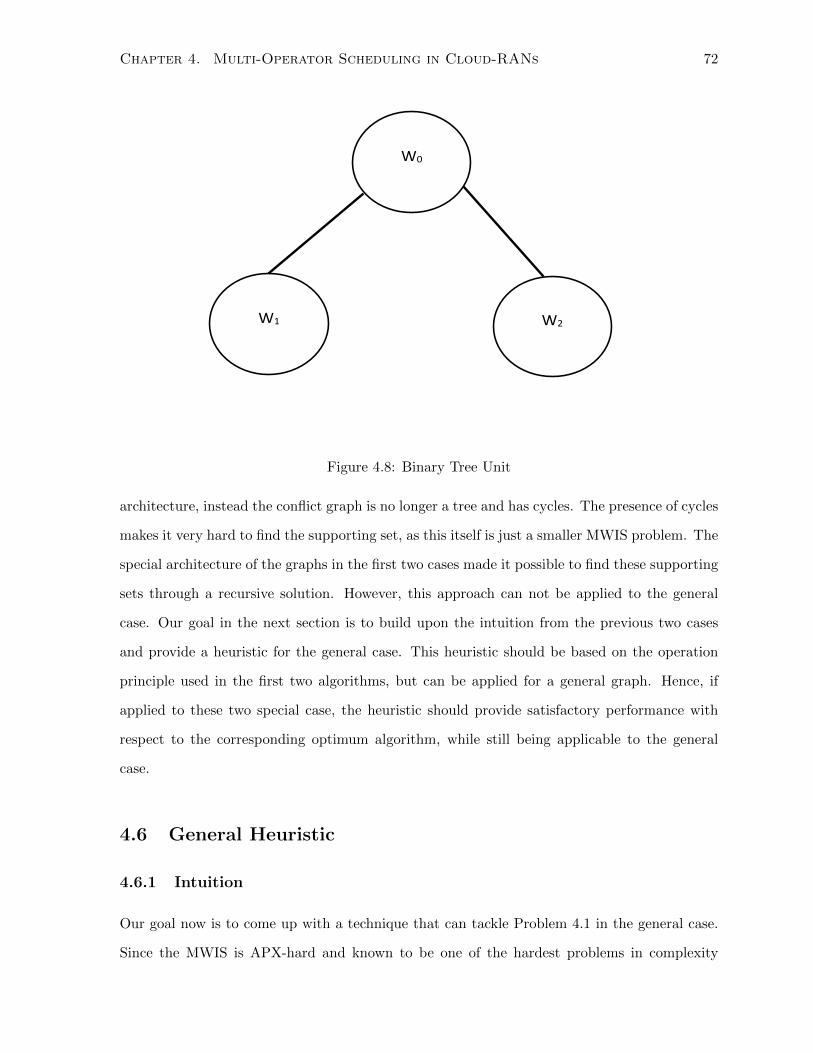
Chapter 4. Multi-Operator Scheduling in Cloud-RANs 72
W0
W1 W2
Figure 4.8: Binary Tree Unit
architecture, instead the conflict graph is no longer a tree and has cycles. The presence of cycles
makes it very hard to find the supporting set, as this itself is just a smaller MWIS problem. The
special architecture of the graphs in the first two cases made it possible to find these supporting
sets through a recursive solution. However, this approach can not be applied to the general
case. Our goal in the next section is to build upon the intuition from the previous two cases
and provide a heuristic for the general case. This heuristic should be based on the operation
principle used in the first two algorithms, but can be applied for a general graph. Hence, if
applied to these two special case, the heuristic should provide satisfactory performance with
respect to the corresponding optimum algorithm, while still being applicable to the general
case.
4.6 General Heuristic
4.6.1 Intuition
Our goal now is to come up with a technique that can tackle Problem 4.1 in the general case.
Since the MWIS is APX-hard and known to be one of the hardest problems in complexity
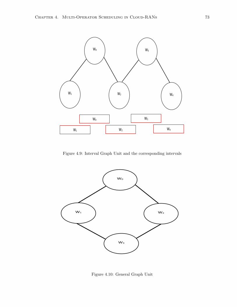
Chapter 4. Multi-Operator Scheduling in Cloud-RANs 73
W0
W1 W2
W3
W4
W1
W0
W2
W3
W4
Figure 4.9: Interval Graph Unit and the corresponding intervals
W0
W1 W2
W3
Figure 4.10: General Graph Unit
Chapter 4. Multi-Operator Scheduling in Cloud-RANs 74
theory [52],[20], the criteria we follow to measure the performance of any algorithm is how it
performs in comparison to the optimum algorithms in their special graphs. The way we design
our heuristic is by looking again at the previous cases and trying to gain insights into how and
why these cases had polynomial time optimum solutions.
The main insight we get from these algorithm is that a set of non-conflicting nodes each
with a small weight should be chosen over a single node with a large weight, if this large node
happens to be conflicting with that set of nodes. Note that this idea is in contrast with the
greedy approach, which usually starts by selecting the node with the largest weight. Hence, it
is necessary for each node to find an approximation for the supporting set of non-conflicting
nodes that support it against the set of conflicting nodes. Note that this is also why the
problem is so hard in the general case, as finding such sets is itself a MWIS, just on a smaller
set. In the special cases we discussed, the key idea was to be able to solve these smaller
MWIS efficiently by imposing some constraints on the graph, hence a recursive algorithm with
polynomial complexity was possible.
4.6.2 Operation
The operation of the algorithm is summarized in Algorithm 4.2. The max(.) can be either a soft-
max or a hardmax. We use the softmax in the proof of convergence. The algorithm can be seen
as equipping each node with a neuron. The neuron’s activation function is w0i
(12 + 1
2 tanh(.)),
where w0i is the initial weight associated with the request. At convergence, the output from the
neuron is either zero or woi . The input to the neuron is composed of:
1. Positive Input: the current weight of the node, plus the sum of the maximum weights
of each set of conflicting support nodes. In other words, for each set of supporting nodes
that are in conflict, we select the one with the maximum weight.
2. Negative Input: the maximum weight among all nodes in conflict with the current node.
The weight for each such node is found in a way similar to the positive input, where the
node’s weight is added together with the sum of the maximum supporting sets.
Theorem 4. If wi <23 ∀i ∈ V, then Algorithm 4.2 converges to a unique fixed point.
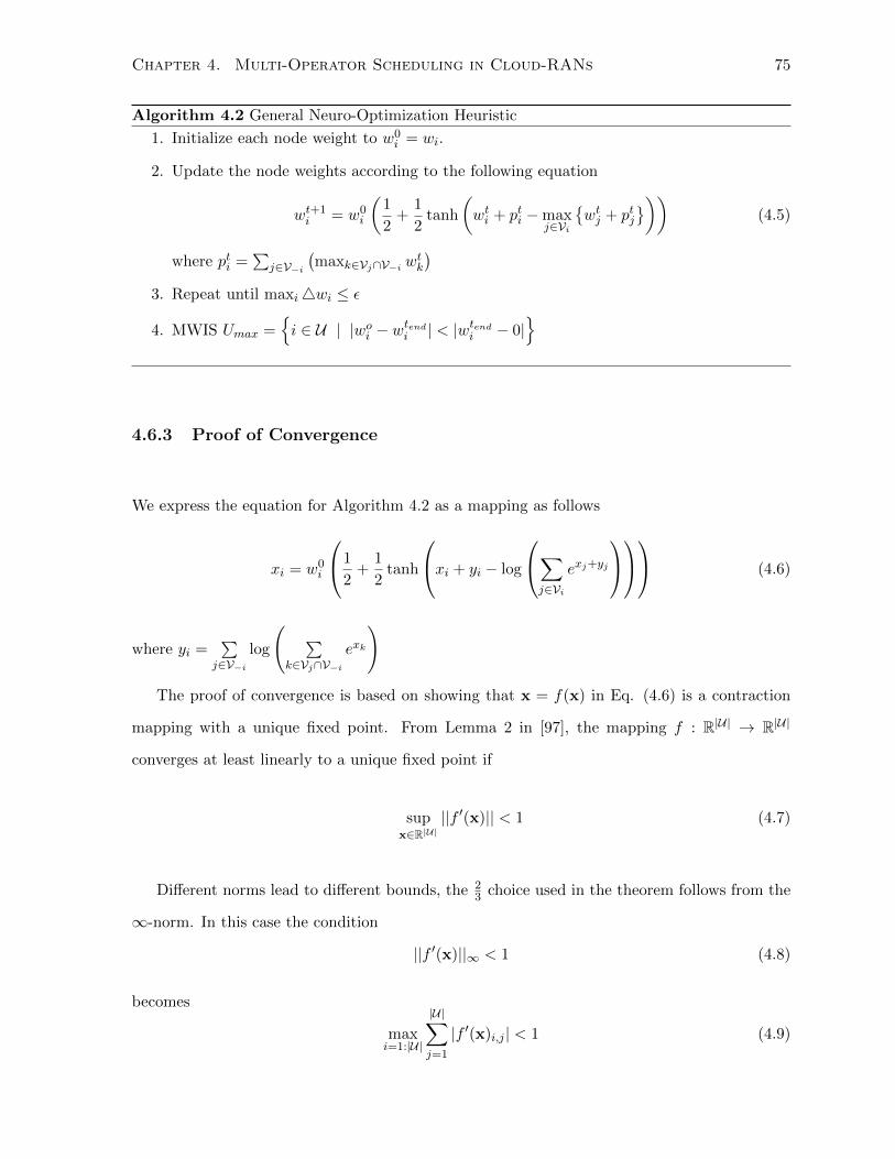
Chapter 4. Multi-Operator Scheduling in Cloud-RANs 75
Algorithm 4.2 General Neuro-Optimization Heuristic
1. Initialize each node weight to w0i = wi.
2. Update the node weights according to the following equation
wt+1i = w0
i
(1
2+
1
2tanh
(wti + pti −max
j∈Vi
{wtj + ptj
}))(4.5)
where pti =∑
j∈V−i(maxk∈Vj∩V−i w
tk
)3. Repeat until maxi4wi ≤ ε
4. MWIS Umax ={i ∈ U | |woi − w
tendi | < |wtendi − 0|
}
4.6.3 Proof of Convergence
We express the equation for Algorithm 4.2 as a mapping as follows
xi = w0i
1
2+
1
2tanh
xi + yi − log
∑j∈Vi
exj+yj
(4.6)
where yi =∑
j∈V−ilog
( ∑k∈Vj∩V−i
exk
)The proof of convergence is based on showing that x = f(x) in Eq. (4.6) is a contraction
mapping with a unique fixed point. From Lemma 2 in [97], the mapping f : R|U| → R|U|
converges at least linearly to a unique fixed point if
supx∈R|U|
||f ′(x)|| < 1 (4.7)
Different norms lead to different bounds, the 23 choice used in the theorem follows from the
∞-norm. In this case the condition
||f ′(x)||∞ < 1 (4.8)
becomes
maxi=1:|U|
|U|∑j=1
|f ′(x)i,j | < 1 (4.9)
Chapter 4. Multi-Operator Scheduling in Cloud-RANs 76
w0
w1
w2
w3
w4
w5
Figure 4.11: Request pattern: s0 = {0, 1, 3}, s1 = {0}, s2 = {1, 3}, s3 = {3}, s4 = {0, 2}, s5 ={1, 2}
Or equivalently|U|∑j=1
|f ′(x)i,j | < 1 ∀i = 1 : |U| (4.10)
Let g(x) = xi + yi − log(∑
j∈Vi exj+yj
). It can be shown that
||f ′(x)||i =
|U|∑j=1
|f ′(x)i,j |
≤ w0i
[1− tanh2(g(x))
]1 +
∑k∈Vj∩V−i
exj∑k∈Vj∩V−i
exj+
∑j∈Vi e
xj+yj∑j∈Vi e
xj+yj
≤ w0
i
[1− tanh2(g(x))
] 3
2≤ w0
i
3
2
(4.11)
Hence, for wi <23 ∀i ∈ V, the mapping is a contraction mapping and convergence is proved. It
is this worth noting that we have this bound to be conservative as our simulations exhibited
convergence without needing to impose this condition on the initial weights.
4.6.4 Neuro-Optimization
A class of optimization techniques related to neural network is known as neuro-optimization.
The most famous of which is the Hopfield network introduced by Hopfield in 1982 [60]. Hopfield
networks are fully-connected neural networks with binary or approximately binary, i.e. sigmoid,
Chapter 4. Multi-Operator Scheduling in Cloud-RANs 77
activation functions. Hopfield networks were used to solve NP-hard combinatorial problems,
such as the traveling salesman problem. The main drawback of Hopfield networks is the large
number of nodes, O(|U|2) needed when solving such combinatorial problem. Our scheme does
not suffer from this problem as we use a number of nodes O(|U|).
4.7 Simulation Results
In this section we present our results regarding the performance of the proposed heuristic in
comparison to the discussed optimum algorithms. The scenario is as explained in the chap-
ter, where the VOs prepare requests for resources and submit them to the coordinator. The
coordinator compares the requests based on the size and weight of each request, and selects a
non-conflicting subset of maximum weight. We vary the number of VOs requests, also called
flows, from 5 to 30. The scheduling weight we use is the channel power gain, where we use
samples from 3GPP LTE channels. Each VO picks the best subset of resources based on the
channel and with randomly chosen sizes. We also compare the proposed algorithms with linear
programming (LP). However, the complexity of the MWIS problem makes the LP solution
highly inefficient.
The first two algorithms discussed are provably optimal for the two special cases. The
main advantage of the third heuristic is its applicability for the general case. The goal of the
simulation results provided here is to study its performance in comparison with the optimum
algorithm for each case.
In Fig. 4.12 we compare the performance of Algorithm 4.2 with the proposed optimal
algorithm for case 1, i.e. Algorithm 4.1. By throughput, we mean the sum of the channel power
gains for the selected subset of requests, which is also the weight of the selected independent set.
The figure shows that the proposed heuristic is within just 2.5% from the optimum algorithm.
The loss in throughput is shown in Fig. 4.14.
A similar observation can be seen in Fig. 4.13 for the interval graph case, case 2. However,
the loss in performance here is more due to the increased complexity of the optimum algorithm.
The proposed heuristic is within 6% from the optimum throughput as shown in Fig. 4.15.
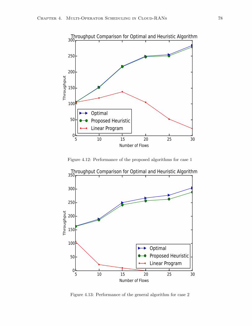
Chapter 4. Multi-Operator Scheduling in Cloud-RANs 78
5 10 15 20 25 30
Number of Flows
0
50
100
150
200
250
300
Throughput
Throughput Comparison for Optimal and Heuristic Algorithm
Optimal
Proposed Heuristic
Linear Program
Figure 4.12: Performance of the proposed algorithms for case 1
5 10 15 20 25 30
Number of Flows
0
50
100
150
200
250
300
350
Throughput
Throughput Comparison for Optimal and Heuristic Algorithm
Optimal
Proposed Heuristic
Linear Program
Figure 4.13: Performance of the general algorithm for case 2
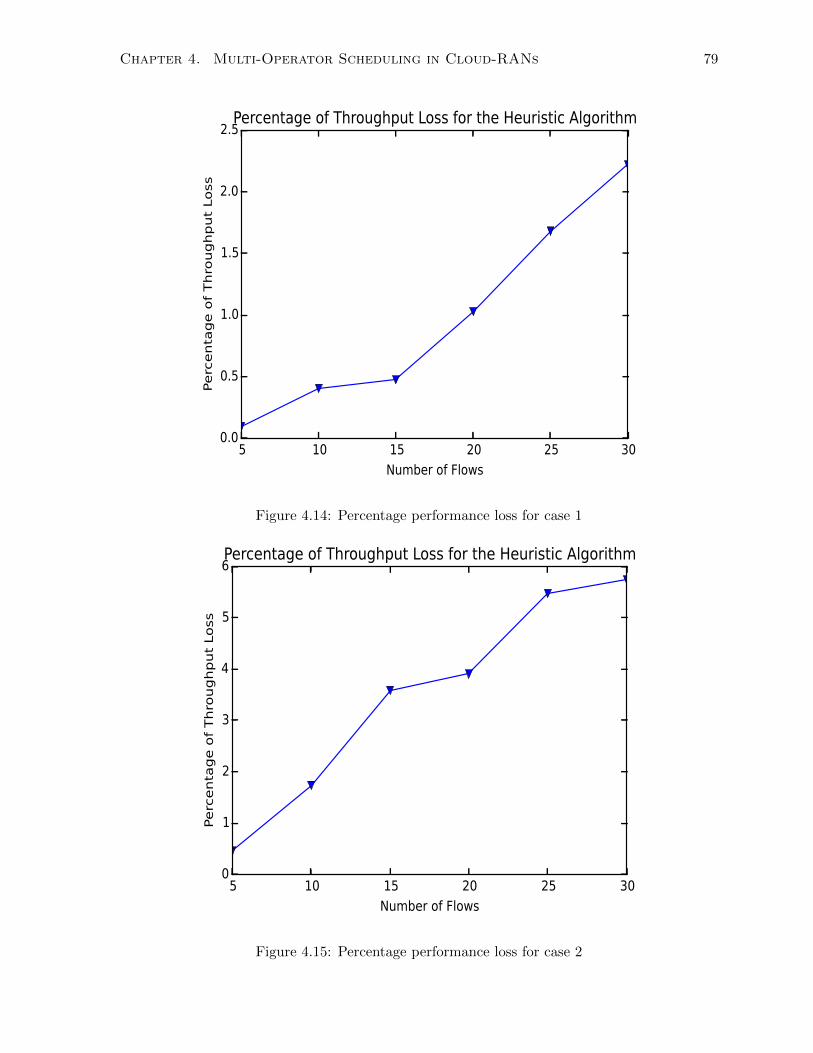
Chapter 4. Multi-Operator Scheduling in Cloud-RANs 79
5 10 15 20 25 30
Number of Flows
0.0
0.5
1.0
1.5
2.0
2.5
Percentage of Throughput Loss
Percentage of Throughput Loss for the Heuristic Algorithm
Figure 4.14: Percentage performance loss for case 1
5 10 15 20 25 30
Number of Flows
0
1
2
3
4
5
6
Percentage of Throughput Loss
Percentage of Throughput Loss for the Heuristic Algorithm
Figure 4.15: Percentage performance loss for case 2
Chapter 4. Multi-Operator Scheduling in Cloud-RANs 80
4.8 Conclusion
In this chapter we have studied the scheduling of multi VOs in a cloud-RAN environment.
We modeled the case when the VOs employ heterogeneous communication protocols. We have
shown that the coordination problem in such a case is in general NP-hard. We then proceeded
by specifying two special cases and provided the optimum algorithm for each case. Finally,
we proposed a novel neuro-computation heuristic, which is able to handle the general problem
but still provide close-to-optimum results for the special cases studied. The simulation results
confirm the effectiveness of the proposed heuristic and help learn more about the operation of
scheduling in cloud-RAN networks. It is worth noting here that such an approach is not the only
to coordinate multiple operators in the same infrastructure, and not necessarily the optimum.
Another possible approach is that IO offers a set of traffic streams which are then utilized by
the VOs. We see this as mainly a trade-off problem, traffic streams offer better utilization,
while forcing all VOs to use the same PHY/MAC technologies. The approach we studied here
was mainly focused on the case where the VOs are heterogeneous. A similar trade-off has also
been seen in the cloud computing field, between virtual machines and containers. While virtual
machines give more flexibility such as choosing different operating systems, they result in lower
utilization compared to containers, which are, on the other hand, much less flexible. There is
no right or wrong approach here, and the choice is to be done per scenario.
Part III
Cloud Computing Challenges
81
82
In the second part of the thesis, we study a set of challenges brought forward by the cloud
computing model itself. The cloud computing model has led to the split of the base band
processing into a user process and a cell process. We study how distributed scheduling can be
used to handle the excessive communication between the two. Next, we study the problem of
resource elasticity and dynamic scaling, for both access and cloud computing resources. For
the access network, we study joint activation, clustering and association of RRHs in a way that
balances energy efficiency with the end-users QoS. For cloud computing, we study the joint
anomaly detection and auto-scaling of the computing resources.
Chapter 5
Fully Distributed Scheduling in
Cloud-RAN Systems
5.1 Context
Cloud Radio Access Networks (C-RAN) promise to leverage cloud computing capabilities for
enhancing the quality and coverage of next generation 5G networks. 5G networks shall witness
an increasing density of users and access points, very small latencies, more bandwidth resources,
and the use of virtualized hardware for baseband processing. Within such an environment, the
problem of scheduling the network users across the radio resources might become a bottleneck
of the system. The cloud computing model has led to the split of the base band processes
into two processes: user process and cell process. However, a new challenge arises due to the
excessive communication needed between the two. In this chapter, we study the design and
performance of distributed schedulers in C-RAN systems. The idea is that each user’s base
band processing unit (BBU) tries to guess whether its user should be scheduled or not. First,
we focus on the case of maximum throughput scheduling and Rayleigh channels, and provide
closed-form expressions for the expected effective channel and signal-to-noise ratio (SNR) in
the distributed scenario. In order to deal with general channels and schedulers, we adopt the
classification techniques from machine learning. We discover an interesting relationship between
the fairness of the scheduler, and its ability to be distributed. In particular, schedulers which
83
Chapter 5. Fully Distributed Scheduling in Cloud-RAN Systems 84
are more fair are also more prune to prediction errors in the distributed scenario. Finally, we
provide simulation results showing that distributed scheduling can provide up to 92% of the
performance of the centralized case.
5.2 Introduction
The concept of cloud-RANs is closely related to that of software-defined networking (SDN) [75]
and network virtualization [32]. Overall, one of the main goals of these technologies is to be
able to support distributed computing capabilities, in the form of data-center servers, as well as
sharing the physical infrastructure between different network operators. The cloud computing
design principles have led to the concepts of distinct user and cell processes within the cloud
RAN architecture. However, such a design has to be considered from the wireless network
perspective. In particular, a central MAC-layer scheduler is needed to coordinate the resource
allocation between the distributed processing units.
One of the main challenges in porting wireless networks to the cloud is the low latency
required in wireless transmission. For example, in LTE a frame has to be sent every millisecond
[119]. Preparing an LTE frame is a computationally expensive process. LTE has adopted two
principles that contribute greatly to its high data rates: channel-selective scheduling and adap-
tive modulation. Scheduling involves selecting a subset of users with relatively good channel
conditions for transmission. Adaptive modulation and coding means choosing the best mod-
ulation and coding scheme for the selected users based on their channel state as well as the
target bit error rate (BER). Revisiting the cloud-RAN architecture, we see that the cell process
is responsible for scheduling the users, while the user process is responsible for the modulation
and coding part. Generally, communication is needed between these two components to come
up with a decision that is as good as the legacy case.
Due to the increasing number of users and RRHs, larger bandwidth and higher PHY layer
complexity, the scheduler is expected to become a heavy performance bottleneck. First, the
needed communication between the processing units and the scheduler is massive. For example,
every time slot, which is 1 ms for LTE and even less is predicted for 5G [17], all users need to
send their information, including channel state information (CSI), to the scheduler. Second,
Chapter 5. Fully Distributed Scheduling in Cloud-RAN Systems 85
even after such information is received, finding the best subset of users is a computationally
expensive task of quadratic complexity [42].
In Fig. 5.1 we show the system architecture as discussed in Chapter 1 focusing on the
scheduling part. In this framework, the base band processing is divided into two parts: user
processing and cell processing. The user process handles all the processing for a single user
such as modulation and coding, while the cell process handles the cell-wide processing such
as the scheduling and the IFFT. Focusing on these two aspects of the cell processing, we can
already see the heavy traffic load between the cell process and the user process. For the IFFT,
the user processes send their I/Q signals for final processing and forwarding to the RRH. For
the scheduler, each user process negotiates with the cell process in order to find whether its
respective user has been selected for transmission within the next time slot. However, this
decision typically involves information such as the CSI of the user and its queue occupancy,
information that is only available to the user process. Hence, the scheduling process already
requires at least two way communication, first the user process forwards its user info to the
scheduler, which then replies with the scheduling decision. Additional communication might
also be needed as more complex features of the scheduler are considered such as the contiguous
band requirements in LTE uplink. These challenges raise an important questions: What happens
if we remove the central scheduler altogether and make the process completely distributed ?
In summary, within the centralized framework, the BBUs communicate with the central
scheduler for the final scheduling decision. This process might involve an initial request, plus
some further negotiations depending on the degree of conflict between the requests from the
different BBUs. All this communication must be finished in less than one transmission time
in order to accommodate some time for the PHY layer processing. We can see that this com-
munication is a very demanding process. Within the distributed architecture, this extensive
communication is non-existent, and the goal of this chapter is to understand how much perfor-
mance we can get.
In this chapter, we study the fully distributed scheduling in Cloud-RAN systems. We model
the distributed scheduling within a C-RAN system and discuss the differences between C-RAN
systems and the existing approaches. Next, we study the maximum throughput scheduling
in Rayleigh channels. We equip each BBU with a predetermined threshold. A BBU would
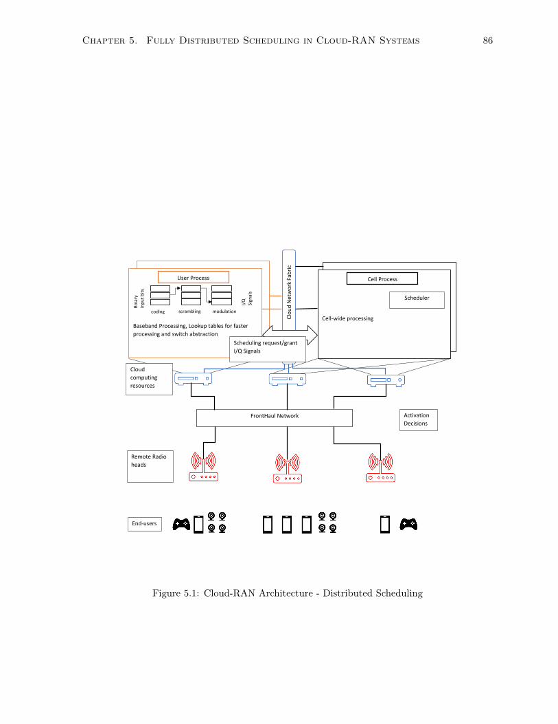
Chapter 5. Fully Distributed Scheduling in Cloud-RAN Systems 86
Baseband Processing, Lookup tables for faster
processing and switch abstraction
Baseband Processing, Lookup tables for faster
processing and switch abstraction
Baseband Processing, Lookup tables for faster
processing and switch abstraction
FrontHaul Network
coding scrambling modulation
Bin
ary
inp
ut
bit
s
I/Q
Sign
als
Cloud
computing
resources
Remote Radio
heads
Cell-wide processing
User Process Cell Process
Scheduler
C
lou
d N
etw
ork
Fab
ric
Activation
Decisions
Scheduling request/grant
I/Q Signals
End-users
Figure 5.1: Cloud-RAN Architecture - Distributed Scheduling
Chapter 5. Fully Distributed Scheduling in Cloud-RAN Systems 87
schedule its user if and only if its channel power gain exceeds the threshold. We provide
closed form expressions for the expected channel gain and SNR as a function of the threshold.
This expression can be maximized to get the optimum threshold value. We then study other
scheduling frameworks, such as proportional fairness and mean-variance maximization. In
these general cases, we use the classification techniques such as support vector machines (SVM)
and Decision Trees to learn the centralized scheduling decisions. Interestingly, we find that
schedulers that are more fair, are also harder to classify and predict. In general, our simulation
results show that up to 92% of the centralized performance can be obtained from the fully
distributed case.
5.3 Related Work
Scheduling for virtual wireless networks has recently received significant attention in the lit-
erature. The NVS prototype developed by NEC Labs proposed to use a two-level hierarchal
scheduling scheme [114]. In the first level, a virtual operator (VO) is selected, and in the second
level, a flow belonging to the selected VO is chosen for transmission based on some parameters
in the service level agreement (SLA) between the VO and the infrastructure owner (IO). A
stochastic game framework was discussed in [46], where an auction determines which VOs get
which resources. The team at University of Bremen has proposed a Hypervisor-like architecture
for LTE virtualization [160], and discussed the scheduling framework within it. Opportunistic
techniques for spectrum sharing among VOs was discussed in [154]. A related line of effort
is concerning with the extension of the network embedding problem into the wireless domain.
[155] is an example of these effort where an on-line scheduling algorithm was proposed based on
Karnaugh maps. However, these works have focused on scheduling multiple VOs on the same
infrastructure, and have not considered the new aspects of the problem related to cloud com-
puting. Specifically, the distributed computation model of the cloud has not been considered
in the current literature. For example, the separation of the user process and the cell process,
the extensive communication needed between the two, and the need, potential as well as design
of distributed approaches for the scheduler design are all absent from the current literature on
cloud-RAN scheduling.
Chapter 5. Fully Distributed Scheduling in Cloud-RAN Systems 88
By transforming the scheduling problem into a distributed decision one, it becomes closer to
a random access problem. The two main approaches in random access are the ALOHA schemes
and the carrier-sensing schemes, known as CSMA [21]. The classical ALOHA approaches have
not considered the effect of the CSI on the system’s performance. The CSI has been integrated
into the system model in more recent works such as [100][64][118][65][151][93]. In [100] and
[151], the problem has been studied assuming successive interference cancellation (SIC) at the
receiver, i.e. collision does not lead to packet loss and multiple users can transmit at the
same time. The authors of [93] have designed a contention resolution scheme where each time
slot is divided into a contention slot and a transmission slot, and the CSI controls the access
probability within the contention slot. Hu et. al [64] have designed a distributed random access
policy using sub-gradient methods to maximize proportional fairness. We extend the ideas of
these works to the cloud-RAN framework.
One of the main differentiators between the cloud-RAN framework and the existing ALOHA
schemes is that a collision in cloud-RAN is not a physical collision due to electromagnetic wave
interference at the receiver as in the case of ALOHA. Instead, it is a logical collision at the cell
process. The assumption that we make is that the cell process keeps a buffer for every resource
block. Whenever a user process decides that its user should transmit on a specific resource
block, it prepares the I/Q signal and forwards it to the corresponding buffer in the cell process.
Either the buffer has enough capacity to store the data for one user only, or the cell process
can simply pick the first signal received. In either case, the existence of the buffer and the fact
that this is a logical rather than physical collision guarantees that the resource block is utilized
if at least one user requested it. The only performance loss will occur if the user selected by
the cell process is not the best one (the cell process is not supposed to decide which user is
picked as we consider fully distributed architectures) or if no user requests the resource block.
These two reasons for performance loss will be considered in our performance analysis later in
the chapter. This aspect of the problem in terms of the different nature of the collision and the
new elements of the cloud-RAN architecture is the main reason why the performance is much
higher compared to the ALOHA case, as will shown.
Chapter 5. Fully Distributed Scheduling in Cloud-RAN Systems 89
5.4 System Model
5.4.1 System Architecture
Consider a cloud-RAN system where a set of virtual machines (VMs) host a set of base band
processors, BBUs. The BBUs forward the I/Q signals through a high-speed network to the
RRHs, where they are transmitted through the air interface to the users’ terminals. In systems
with deterministic access, such as 3G and 4G, a scheduler is responsible for choosing a subset
of users for transmission at each time slot. Within the considered framework, the BBUs are
responsible for calculating the scheduling weights, e.g. channel gain for maximum throughput
and channel gain divided by aggregate throughput for proportional fairness. These weights are
transmitted from the VM where the BBU is located to the VM where the scheduler function is
running. Once the data is received from all BBUs, the scheduling decision is made. Typically,
this is a process of complexity O(|U||S|), where |U| is the number of users and |S| is the number
of resources. Note that this process is repeated every transmission slot, e.g. 1 ms for LTE. We
focus in this chapter on the single cell scenarios, where the scheduling decision is localized at
each cell. Extensions to multi-cell coordinated scheduling is left for future work.
In order to avoid the scheduler becoming a bottleneck for the system, we study in this
chapter what happens if we make the process fully distributed. The architecture we assume
is as follows: the BBUs are still responsible for calculating the scheduling weights as before.
However, there is no central scheduler, each BBU should be able to find out on its own, with
no coordination with the other BBUs, whether its respective user should be scheduled. Finally,
the BBUs prepare the pre-filtered signals, which are sent to a central unit for final filtering
and forwarding to the RRH [53]. We assume that if two or more user are scheduled for the
same resources, one of them is chosen at random before the final filtering process. While this
complete lack of coordination might be a pessimistic assumption, understanding the behavior
in such a case can serve as a lower bound on the performance of other scenarios.
The question then becomes how can the BBU know if its user should be scheduled. If the
criteria is too conservative, only a small number of BBUs will schedule their users, resulting
in underutilized resources. On the other hand, if the criteria is too permissive, many BBUs
will schedule their users, and when one of these users is chosen at random, it might result in
Chapter 5. Fully Distributed Scheduling in Cloud-RAN Systems 90
choosing a less deserving user. Finding the optimal trade-off between these two extremes is the
main optimization problem of this chapter.
5.4.2 Model
Consider a cloud-RAN system where a cloud data center forwards the I/Q signals through a
high-speed network to a set of RRHs. Let S be the set of resources. Let U be the set of
distributed BBUs.
Each BBU u ∈ U prepares a request specifying the desired subset of resources. Let Su
denote such a request. We assume that each request Su is composed of the weights ws,u for
every resource s ∈ S. This weight is used by the central scheduler to compare the different
requests. Different scheduling weights have been discussed in the literature, see [42] for a survey.
In the current work we are not concerned with the design of the scheduling weight, rather we
assume that the BBUs and the scheduler agree upon a specific criteria for determining the
weights. The decision made by the central scheduler is:
us = arg maxu∈U
ws,u (5.1)
where us is the user selected for resource s.
5.5 Distributed Scheduling
5.5.1 Maximum Throughput Rayleigh Channels
In this section, we consider the problem of distributing the maximum throughput scheduler
for users whose channels follow a Rayleigh distribution. We adopt a threshold-based decision
criteria for the BBUs. Each BBU observes the channel vector of its user, compares it with a
predefined threshold value, and based on that decides whether to select the user for transmission.
If two or more users are selected for the same resource, one is chosen at random. For the
maximum throughout scheduling, the user with highest SNR value for each resource is selected.
In the following, we denote by |h|s,u the channel gain for user u at resource s, while |h|s denotes
the channel gain for resource s, i.e. the channel of the selected user. Note that |h|s = 0 if none
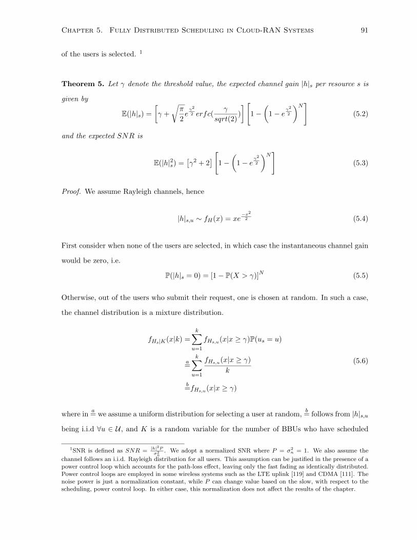
Chapter 5. Fully Distributed Scheduling in Cloud-RAN Systems 91
of the users is selected. 1
Theorem 5. Let γ denote the threshold value, the expected channel gain |h|s per resource s is
given by
E(|h|s) =
[γ +
√π
2eγ2
2 erfc(γ
sqrt(2))
][1−
(1− e
γ2
2
)N](5.2)
and the expected SNR is
E(|h|2s) =[γ2 + 2
] [1−
(1− e
γ2
2
)N](5.3)
Proof. We assume Rayleigh channels, hence
|h|s,u ∼ fH(x) = xe−x22 (5.4)
First consider when none of the users are selected, in which case the instantaneous channel gain
would be zero, i.e.
P(|h|s = 0) = [1− P(X > γ)]N (5.5)
Otherwise, out of the users who submit their request, one is chosen at random. In such a case,
the channel distribution is a mixture distribution.
fHs|K(x|k) =k∑
u=1
fHs,u(x|x ≥ γ)P(us = u)
a=
k∑u=1
fHs,u(x|x ≥ γ)
k
b=fHs,u(x|x ≥ γ)
(5.6)
where ina= we assume a uniform distribution for selecting a user at random,
b= follows from |h|s,u
being i.i.d ∀u ∈ U , and K is a random variable for the number of BBUs who have scheduled
1SNR is defined as SNR = |h|2Pσ2n
. We adopt a normalized SNR where P = σ2n = 1. We also assume the
channel follows an i.i.d. Rayleigh distribution for all users. This assumption can be justified in the presence of apower control loop which accounts for the path-loss effect, leaving only the fast fading as identically distributed.Power control loops are employed in some wireless systems such as the LTE uplink [119] and CDMA [111]. Thenoise power is just a normalization constant, while P can change value based on the slow, with respect to thescheduling, power control loop. In either case, this normalization does not affect the results of the chapter.
Chapter 5. Fully Distributed Scheduling in Cloud-RAN Systems 92
their users for the specific resource s.
fHs(x) =N∑k=1
fHs|K(x|k)P(K = k)
=N∑k=1
fHs|K(x|k)
(N
k
)[P(X > γ)]k [1− P(X > γ)]N−k
c= fHs|K(x|k) [1− P(K = 0)]
= fHs,u(x|x ≥ γ) [1− P(K = 0)]
(5.7)
wherec= follows from fHs|K(x|k) being independent of k as shown in (5.6). Now for Rayleigh
distributions, it can be shown that
fHs,u(x|x ≥ γ) =xe−x22
e−γ22
(5.8)
and
P(K = 0) = [P(X < γ)]N =
(1− e
γ2
2
)N(5.9)
In summary
fHs(x) =
[1− P(X > γ)]N , x = 0
fHs,u(x|x ≥ γ)
[1−
(1− e
γ2
2
)N], x ≥ γ
(5.10)
Note that fHs(x) is undefined for the range 0 < x < γ.
To find E(|h|s)
E(|h|s) = 0 ∗ P(|h|s = 0) +
∫ ∞γ
x× xe−x22
e−γ22
[1−
(1− e
γ2
2
)N](5.11)
leading to
E(|h|s) =
[γ +
√π
2eγ2
2 erfc(γ
sqrt(2))
][1−
(1− e
γ2
2
)N](5.12)
The expression for E(|h|2s) can be found using the same procedure starting from the fact that
Chapter 5. Fully Distributed Scheduling in Cloud-RAN Systems 93
|h|2s is a Chi-square random variable with 2 degrees of freedom, i.e.
|h|2s,u ∼ fH2(z) =1
2e−z2 (5.13)
Since γ∗ = arg maxγ E(log(1 + SNRs(γ))) = arg maxγ E(SNRs(γ)) = arg maxγ E(|h|s(γ)),
by maximizing E(|h|s), we find the optimum value of γ as a function of N and store it in a
lookup table for example
In order to validate our analysis and study the performance of the distributed scheduling,
simulation results are provided in Fig. 5.2 and 5.3. In Fig. 5.2 we show the expected channel
gain and SNR versus γ. It can be seen that the analytical expressions match exactly with the
simulation. A comparison of the expected performance between the centralized and distributed
schedulers is shown in Fig. 5.3 for different numbers of users. We find that the distributed
scheduler can achieve approximately 85% of the SNR performance and 92% of the channel
capacity performance in comparison to the centralized scheduler. We take this value as an
upper bound on the performance of the schemes in the upcoming sections.
5.5.2 General Schedulers and Distributions
In the case of general schedulers and channel distributions, performing an analysis similar to
the one in the previous part might not be feasible. A more systematic approach makes use of
the classification techniques [147] from machine learning to learn the scheduling decisions. Each
BBU will be equipped with a classifier. At each transmission slot, the classifier will determine
whether the BBU should/can transmit at a specific resource block. This decision is based on
some data features such as channel gain and queue size. Note that the classifiers belonging
to different BBUs do not communicate. Hence, the process is completely distributed and no
inter-BBU signaling is needed.
First, the system is to be trained in the presence of a centralized scheduler. BBUs submit
their requests to the scheduler, which performs the user selection decisions. The data involving
the users’ channels and the scheduler’s decisions are used to train the classifier. Once training is
finished, each BBU is provided the trained classifier which then makes the distributed decision.
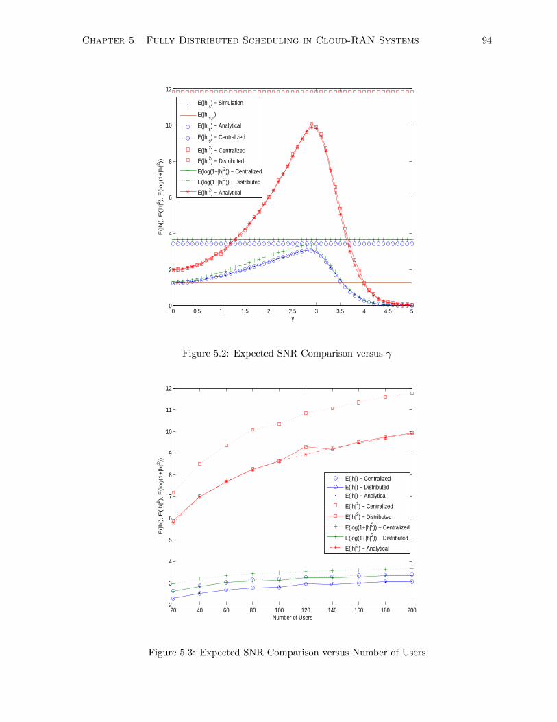
Chapter 5. Fully Distributed Scheduling in Cloud-RAN Systems 94
0 0.5 1 1.5 2 2.5 3 3.5 4 4.5 50
2
4
6
8
10
12
γ
E(|
h|)
, E
(|h
|2),
E(lo
g(1
+|h
|2))
E(|h|s) − Simulation
E(|h|s,u
)
E(|h|s) − Analytical
E(|h|s) − Centralized
E(|h|2) − Centralized
E(|h|2) − Distributed
E(log(1+|h|2)) − Centralized
E(log(1+|h|2)) − Distributed
E(|h|2) − Analytical
Figure 5.2: Expected SNR Comparison versus γ
20 40 60 80 100 120 140 160 180 2002
3
4
5
6
7
8
9
10
11
12
Number of Users
E(|
h|)
, E
(|h
|2),
E(lo
g(1
+|h
|2))
E(|h|) − CentralizedE(|h|) − DistributedE(|h|) − Analytical
E(|h|2) − Centralized
E(|h|2) − Distributed
E(log(1+|h|2)) − Centralized
E(log(1+|h|2)) − Distributed
E(|h|2) − Analytical
Figure 5.3: Expected SNR Comparison versus Number of Users
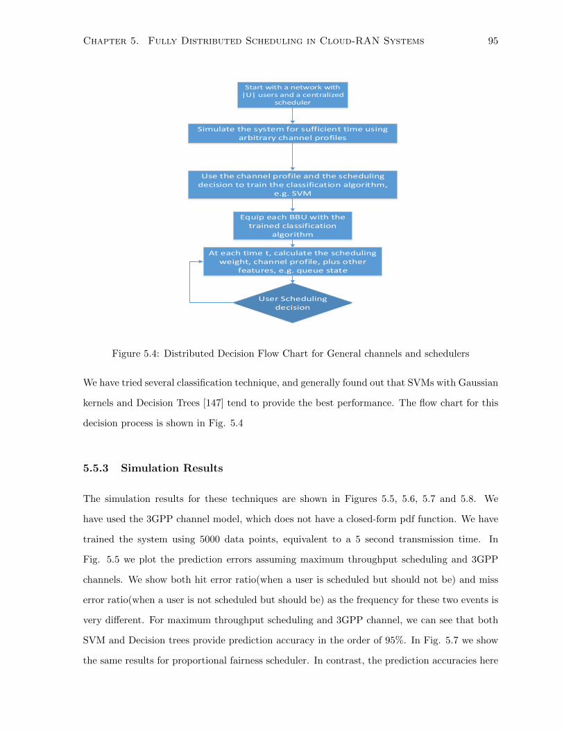
Chapter 5. Fully Distributed Scheduling in Cloud-RAN Systems 95
Start with a network with |U| users and a centralized
scheduler
Simulate the system for sufficient time using arbitrary channel profiles
Use the channel profile and the scheduling decision to train the classification algorithm,
e.g. SVM
Equip each BBU with the trained classification
algorithm
User Scheduling decision
At each time t, calculate the scheduling weight, channel profile, plus other
features, e.g. queue state
Figure 5.4: Distributed Decision Flow Chart for General channels and schedulers
We have tried several classification technique, and generally found out that SVMs with Gaussian
kernels and Decision Trees [147] tend to provide the best performance. The flow chart for this
decision process is shown in Fig. 5.4
5.5.3 Simulation Results
The simulation results for these techniques are shown in Figures 5.5, 5.6, 5.7 and 5.8. We
have used the 3GPP channel model, which does not have a closed-form pdf function. We have
trained the system using 5000 data points, equivalent to a 5 second transmission time. In
Fig. 5.5 we plot the prediction errors assuming maximum throughput scheduling and 3GPP
channels. We show both hit error ratio(when a user is scheduled but should not be) and miss
error ratio(when a user is not scheduled but should be) as the frequency for these two events is
very different. For maximum throughput scheduling and 3GPP channel, we can see that both
SVM and Decision trees provide prediction accuracy in the order of 95%. In Fig. 5.7 we show
the same results for proportional fairness scheduler. In contrast, the prediction accuracies here
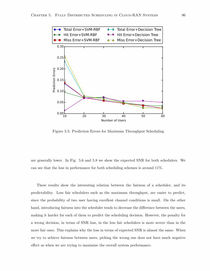
Chapter 5. Fully Distributed Scheduling in Cloud-RAN Systems 96
10 20 30 40 50 60
Number of Users
0.00
0.05
0.10
0.15
0.20
0.25
0.30
Prediction Errors
Total Error+SVM-RBF
Hit Error+SVM-RBF
Miss Error+SVM-RBF
Total Error+Decision Tree
Hit Error+Decision Tree
Miss Error+Decision Tree
Figure 5.5: Prediction Errors for Maximum Throughput Scheduling
are generally lower. In Fig. 5.6 and 5.8 we show the expected SNR for both schedulers. We
can see that the loss in performance for both scheduling schemes is around 11%.
These results show the interesting relation between the fairness of a scheduler, and its
predictability. Less fair schedulers such as the maximum throughput, are easier to predict,
since the probability of two user having excellent channel conditions is small. On the other
hand, introducing fairness into the scheduler tends to decrease the difference between the users,
making it harder for each of them to predict the scheduling decision. However, the penalty for
a wrong decision, in terms of SNR loss, in the less fair schedulers is more severe than in the
more fair ones. This explains why the loss in terms of expected SNR is almost the same. When
we try to achieve fairness between users, picking the wrong one does not have much negative
effect as when we are trying to maximize the overall system performance.
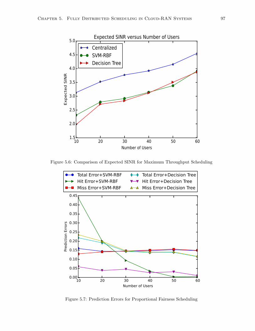
Chapter 5. Fully Distributed Scheduling in Cloud-RAN Systems 97
10 20 30 40 50 60
Number of Users
1.5
2.0
2.5
3.0
3.5
4.0
4.5
5.0
Expected SINR
Expected SINR versus Number of Users
Centralized
SVM-RBF
Decision Tree
Figure 5.6: Comparison of Expected SINR for Maximum Throughput Scheduling
10 20 30 40 50 60
Number of Users
0.00
0.05
0.10
0.15
0.20
0.25
0.30
0.35
0.40
0.45
Prediction Errors
Total Error+SVM-RBF
Hit Error+SVM-RBF
Miss Error+SVM-RBF
Total Error+Decision Tree
Hit Error+Decision Tree
Miss Error+Decision Tree
Figure 5.7: Prediction Errors for Proportional Fairness Scheduling
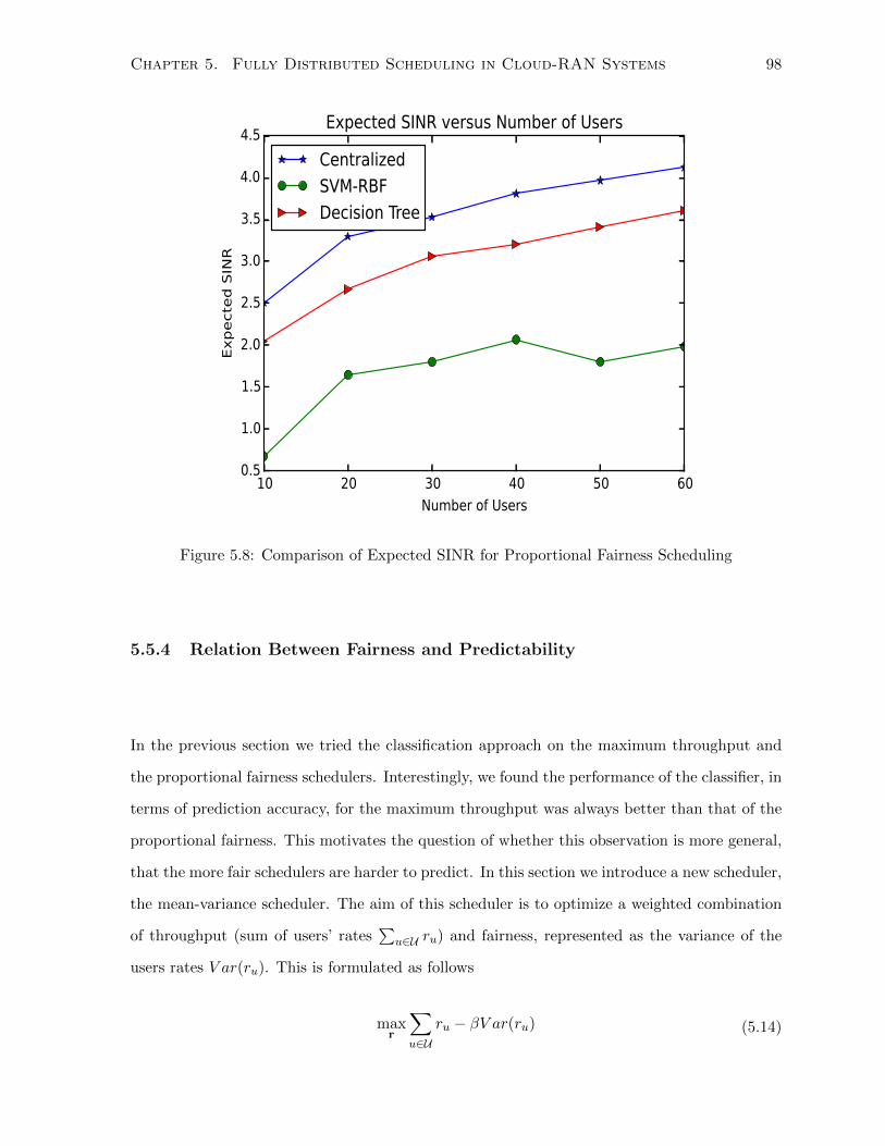
Chapter 5. Fully Distributed Scheduling in Cloud-RAN Systems 98
10 20 30 40 50 60
Number of Users
0.5
1.0
1.5
2.0
2.5
3.0
3.5
4.0
4.5
Expected SINR
Expected SINR versus Number of Users
Centralized
SVM-RBF
Decision Tree
Figure 5.8: Comparison of Expected SINR for Proportional Fairness Scheduling
5.5.4 Relation Between Fairness and Predictability
In the previous section we tried the classification approach on the maximum throughput and
the proportional fairness schedulers. Interestingly, we found the performance of the classifier, in
terms of prediction accuracy, for the maximum throughput was always better than that of the
proportional fairness. This motivates the question of whether this observation is more general,
that the more fair schedulers are harder to predict. In this section we introduce a new scheduler,
the mean-variance scheduler. The aim of this scheduler is to optimize a weighted combination
of throughput (sum of users’ rates∑
u∈U ru) and fairness, represented as the variance of the
users rates V ar(ru). This is formulated as follows
maxr
∑u∈U
ru − βV ar(ru) (5.14)
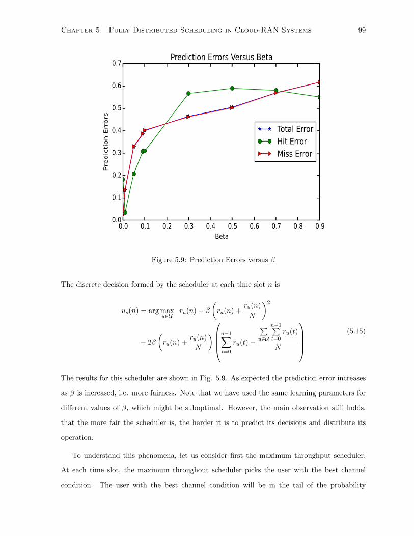
Chapter 5. Fully Distributed Scheduling in Cloud-RAN Systems 99
0.0 0.1 0.2 0.3 0.4 0.5 0.6 0.7 0.8 0.9
Beta
0.0
0.1
0.2
0.3
0.4
0.5
0.6
0.7
Prediction Errors
Prediction Errors Versus Beta
Total Error
Hit Error
Miss Error
Figure 5.9: Prediction Errors versus β
The discrete decision formed by the scheduler at each time slot n is
us(n) = arg maxu∈U
ru(n)− β(ru(n) +
ru(n)
N
)2
− 2β
(ru(n) +
ru(n)
N
)n−1∑t=0
ru(t)−
∑u∈U
n−1∑t=0
ru(t)
N
(5.15)
The results for this scheduler are shown in Fig. 5.9. As expected the prediction error increases
as β is increased, i.e. more fairness. Note that we have used the same learning parameters for
different values of β, which might be suboptimal. However, the main observation still holds,
that the more fair the scheduler is, the harder it is to predict its decisions and distribute its
operation.
To understand this phenomena, let us consider first the maximum throughput scheduler.
At each time slot, the maximum throughout scheduler picks the user with the best channel
condition. The user with the best channel condition will be in the tail of the probability
Chapter 5. Fully Distributed Scheduling in Cloud-RAN Systems 100
distribution, i.e. a high value for the channel magnitude which occurs with very low probability.
However, if the number of users is large enough, then we expect to have one such user at
almost every time slot. Since this best user user is far from the channel values with significant
probability, the data is relatively separable and the classifier can learn a good decision boundary.
In other words, there is enough probability to have one user with a very good channel condition
, but very low probability of having two such users, hence the data becomes separable.
Now let us look at the other extreme, schedulers that are focused solely on fairness. One such
scheduler is the round-robin, where all users get equal access to the resources irrespective of their
channel condition. The round-robin scheduler is statistically equivalent to a uniformly random
scheduler, where each is used is picked with equal probability. In both cases, the resources are
divided equally between the users. However, there is no information in the uniformly random
scheduler, and hence no classifier can learn to model its behavior. The means that fully fair
schedulers are not predictable. Since the proportional fairness scheduler lies somewhere between
the maximum throughput and the fully fair scheduler, we can see now why it is harder to predict
its decisions compared with the maximum throughput schedulers.
5.6 Conclusion
In this chapter we have studied the distributed scheduling problem in Cloud-RAN systems.
Analytical analysis for the Rayleigh channels and maximum throughput scheduler is provided.
We found that distributed scheduling in this case is able to provide around 92% of the centralized
performance. We then extended the scheme to general channels and schedulers by adopting
the classification techniques from machine learning. We discovered two conflicting effects that
depend upon the fairness of the scheduler. In particular, more fair schedulers are easier to
predict, but the penalty for wrong decisions is more severe. With enough training and efficient
parameter selection, the distributed schedulers are able to provide up to 89% of the centralized
performance.
Chapter 6
Joint RRH Activation and
Clustering in Cloud-RANs
6.1 Context
Cloud Radio Access Networks (Cloud-RAN) promise to leverage cloud computing capabilities to
enhance the quality and coverage of wireless networks. A dense network of remote radio heads
(RRHs) ensures less attenuation at the receiver side. However, two drawbacks are associated
with such dense network: the first is the high energy consumption associated with the large
number of RRHs; the second is the interference experienced by the receiver due to the close
proximity of the transmitters. The cloud-RAN must adopt the cloud design principles such
as resource elasticity and dynamic scaling. The infrastructure controller is responsible for
controlling the access network through activation and clustering of RRHs. The decisions made
by the infrastructure controller are based on the information it receives from the user processes
and should balance energy efficiency with the QoS received by the users. Hence, in this chapter
we study the problem of joint activation and clustering of RRHs. Since the problem is NP-
hard, we provide a two-step algorithm that can find an efficient solution. The first step uses
linear-programming relaxation to find a feasible solution. The second step is a greedy approach
to improve the utility function through gradual activation-clustering of RRHs. Our simulation
results demonstrate the benefit in the joint design of activation and clustering over existing
101
Chapter 6. Joint RRH Activation and Clustering in Cloud-RANs 102
activation only approaches.
6.2 Introduction
Energy efficiency is one of the main goals of cloud RAN. Current studies estimate that the
information and communication technology (ICT) sector contributes around 2% of the global
CO2 emissions [94], [86]. This carbon footprint is expected to triple by 2020 as a result of
the massive growth of cellular traffic. From the network operators perspective, building more
energy-efficient systems not only lowers their carbon footprint, but is also of significant economic
benefit as it saves their expenditure on energy bills. Considering that around 60-80% of the
energy consumption in a cellular network is consumed at the base-stations [87], [130], it is
no surprise that the C-RAN architecture tries to come up with more energy-efficient network
architectures.
The C-RAN architecture succeeds in decreasing one aspect of energy consumption, which is
related to the cooling and infrastructure of the macro base stations used in the current systems.
However, the energy consumption due to transmission is still present, and might even increase
due to the large number of RRHs envisioned in C-RAN systems. An important question then
becomes, given the high-redundancy of transmitters associated with the dense installation of
RRHs, how to select only a subset of these RRH in order to satisfy the users’ needs while
keeping the energy consumption to a minimum.
Interference is another important factor in the design of cloud RAN systems. The high
density of RRHs results in a decrease in the signal to interference and noise ratio (SINR). Co-
ordinated Multi-Point Transmission (CoMP) is a family of cooperative transmission techniques
that is well studied in cellular systems [50]. A main idea of CoMP is to cluster transmitters
together into a cooperative transmission set in order to coordinate their transmission. Hence,
clustering RRHs together results in improved SINR at the user side, which can be utilized to de-
activate some RRHs in order to save energy. However, in cloud RAN systems, users’ baseband
processing is performed in servers located in data centers, and the mutual exchange of data as
required by CoMP is governed by the networking infrastructure of these data centers. Hence,
any clustering scheme should strike an efficient trade-off between the users’ SINR distribution
Chapter 6. Joint RRH Activation and Clustering in Cloud-RANs 103
and the bandwidth consumption of the underlying networking infrastructure.
In Fig. 6.1 we show the system architecture focused on the access network control part. The
main part under study is the activation and clustering decisions by the infrastructure controller.
The infrastructure controller monitors the state of the network through continuously receiving
updates from the user process about the states of their users, eh.g. position, queue occupancy
and SINR. Based on this information, the infrastructure controller can then decide to activate
or de-activate a set of RRHs. Clearly, the activation decision is taken when a set of user within
close proximity to an inactive RRH are receiving an inadequate level of service. Similarly, the de-
activation is taken when the infrastructure controller can identify part of the network with low
enough density of users such that they can be migrated to another RRH without affecting their
QoS. The decisions made the infrastructure controller are about balancing the energy efficiency
of the network with the QoS achieved by the end users. Crucial to the infrastructure controller
decisions is the notion of clustering. Two RRHs can be clustered such that together they can
provide an acceptable level of service to the user of a third inactive RRH. The infrastructure
communicates this clustering decision to the corresponding cell processes in order to have them
coordinate their transmission together. FInally, The infrastructure controller communicates
with the RRHs by giving them the activation/de-activation decisions. The capabilities of the
cloud-RAN architecture, such as the collocation of the base band processing in the cloud and
the central management of the network through the infrastructure controller, are great enablers
for these clustering-enhanced activation decisions.
6.3 Related Work
In [133], the authors studied the base station deployment problem together with switching
ON/OFF some of them in order to guarantee QoS for the users. They used area spectral
efficiency [14] as their main QoS metric, and proposed a simple deterministic greedy algorithm
for the deployment and operation of the base stations. [108] introduced the idea of spatio-
temporal profiling to select an active subset of base stations for each duration. Cooperative
communication was used in [55] to accommodate the users whose base stations are turned off.
[104] introduced the concept of network impact to measure the effect of switching OFF a base
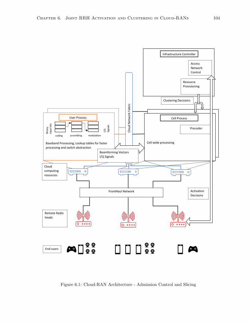
Chapter 6. Joint RRH Activation and Clustering in Cloud-RANs 104
Baseband Processing, Lookup tables for faster
processing and switch abstraction
Baseband Processing, Lookup tables for faster
processing and switch abstraction
Baseband Processing, Lookup tables for faster
processing and switch abstraction
FrontHaul Network
coding scrambling modulation
Bin
ary
inp
ut
bit
s
I/Q
Sign
als
Cloud
computing
resources
Remote Radio
heads
Cell-wide processing
User Process Cell Process
Precoder
Infrastructure Controller
Resource
Provisioning
Clo
ud
Net
wo
rk F
abri
c
Clustering Decisions
Access
Network
Control
Activation
Decisions
Beamforming Vectors
I/Q Signals
End-users
Figure 6.1: Cloud-RAN Architecture - Admission Control and Slicing
Chapter 6. Joint RRH Activation and Clustering in Cloud-RANs 105
station on its neighbors, and used it to build heuristics for gradual base station activation.
The joint deployment and operation problem was studied in [132], and greedy algorithms have
been proposed for both problems. An analysis and optimization approach based on stochastic
geometry was performed in [124], where two BSs sleeping strategies were studied. The energy-
delay trade-off was studied in [131]. Finally, antenna switching was distinguished from base
station switching in [163], which introduced both dynamic and semi-dynamic solutions for the
problem.
The main drawback of current studies is the absence of the clustering effect on the clustering
decisions. This is more crucial in the cloud-RAN architectures due to the high density of the
RRHs as mentioned before. Hence, our main goal in this chapter is to study how can the
clustering effect/decisions be incorporated into the RRH activation problem.
We improve upon the existing literature as follows: first, we introduce a coverage constraint
to the problem formulation in order to ensure connectivity for all users, and to avoid the waste
of resources associated with connection establishment and termination, which will occur due to
blindly turning off some RRHs. The second contribution is in the modeling of the users’ QoS.
While previous attempts have focused on SINR as the QoS metric, they ignored the higher-layer
metrics such as the number of users and the division of resources between them. Even if a user
achieves high SINR, its overall QoS still depends on how many resource blocks, bandwidth,
it can get. The third and main contribution is to consider RRH clustering jointly with RRH
activation. The reason for this is that it might be enough to cluster two RRHs together to
cover the area of a third RRH, without turning on that third RRH, hence saving energy.
6.4 System Model
6.4.1 System Description
Network Model
Consider a cloud-RAN system where a cloud data center forwards the I/Q signals through a
high-speed network to a set of RRHs. Let R be the set of RRHs, U the set of users, T the set
of time slots and C the set of RRHs clusters.
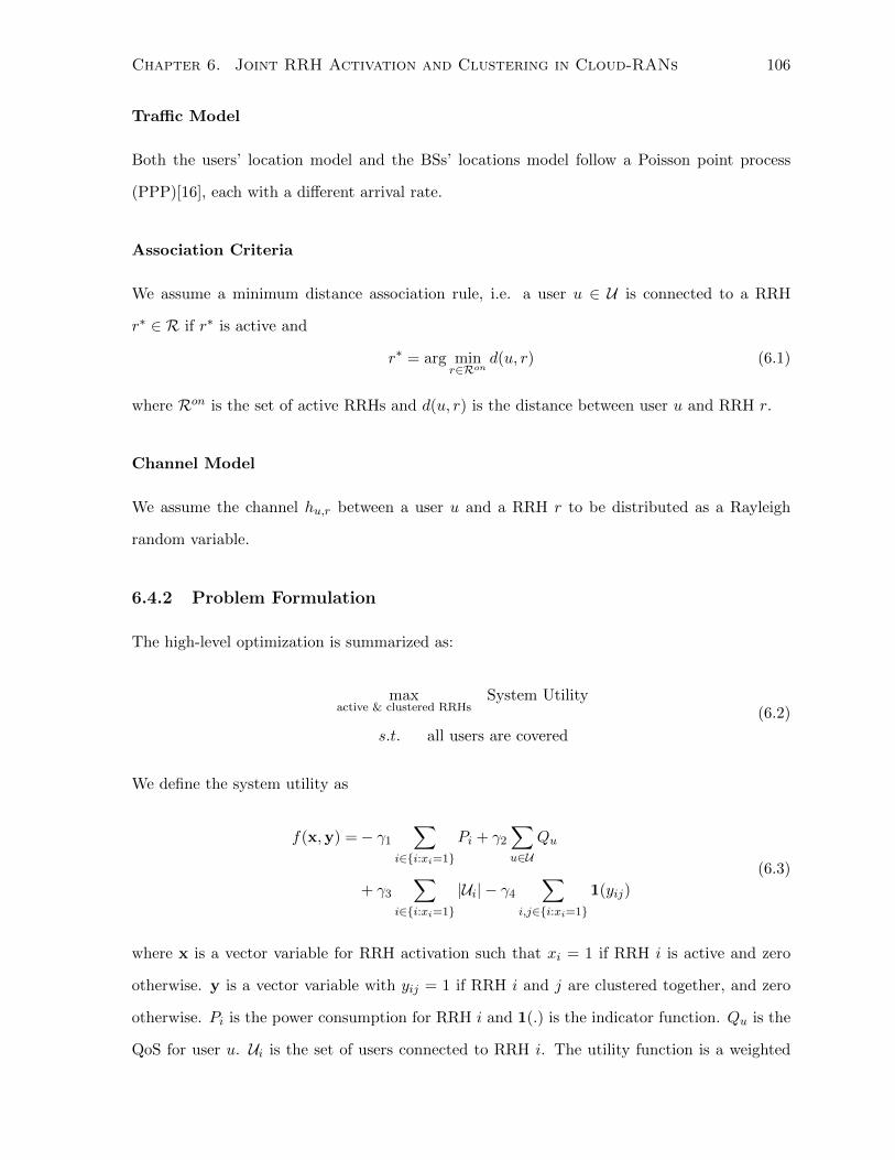
Chapter 6. Joint RRH Activation and Clustering in Cloud-RANs 106
Traffic Model
Both the users’ location model and the BSs’ locations model follow a Poisson point process
(PPP)[16], each with a different arrival rate.
Association Criteria
We assume a minimum distance association rule, i.e. a user u ∈ U is connected to a RRH
r∗ ∈ R if r∗ is active and
r∗ = arg minr∈Ron
d(u, r) (6.1)
where Ron is the set of active RRHs and d(u, r) is the distance between user u and RRH r.
Channel Model
We assume the channel hu,r between a user u and a RRH r to be distributed as a Rayleigh
random variable.
6.4.2 Problem Formulation
The high-level optimization is summarized as:
maxactive & clustered RRHs
System Utility
s.t. all users are covered
(6.2)
We define the system utility as
f(x,y) =− γ1∑
i∈{i:xi=1}
Pi + γ2∑u∈U
Qu
+ γ3∑
i∈{i:xi=1}
|Ui| − γ4∑
i,j∈{i:xi=1}
1(yij)
(6.3)
where x is a vector variable for RRH activation such that xi = 1 if RRH i is active and zero
otherwise. y is a vector variable with yij = 1 if RRH i and j are clustered together, and zero
otherwise. Pi is the power consumption for RRH i and 1(.) is the indicator function. Qu is the
QoS for user u. Ui is the set of users connected to RRH i. The utility function is a weighted
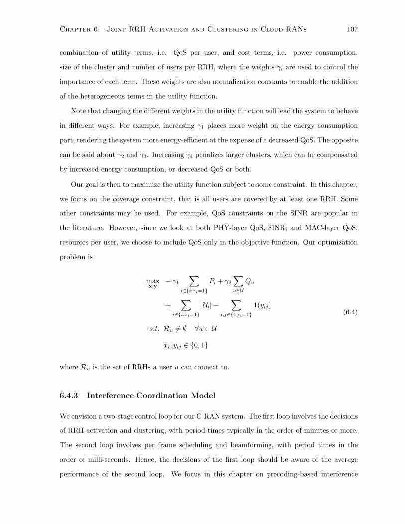
Chapter 6. Joint RRH Activation and Clustering in Cloud-RANs 107
combination of utility terms, i.e. QoS per user, and cost terms, i.e. power consumption,
size of the cluster and number of users per RRH, where the weights γi are used to control the
importance of each term. These weights are also normalization constants to enable the addition
of the heterogeneous terms in the utility function.
Note that changing the different weights in the utility function will lead the system to behave
in different ways. For example, increasing γ1 places more weight on the energy consumption
part, rendering the system more energy-efficient at the expense of a decreased QoS. The opposite
can be said about γ2 and γ3. Increasing γ4 penalizes larger clusters, which can be compensated
by increased energy consumption, or decreased QoS or both.
Our goal is then to maximize the utility function subject to some constraint. In this chapter,
we focus on the coverage constraint, that is all users are covered by at least one RRH. Some
other constraints may be used. For example, QoS constraints on the SINR are popular in
the literature. However, since we look at both PHY-layer QoS, SINR, and MAC-layer QoS,
resources per user, we choose to include QoS only in the objective function. Our optimization
problem is
maxx,y
− γ1∑
i∈{i:xi=1}
Pi + γ2∑u∈U
Qu
+∑
i∈{i:xi=1}
|Ui| −∑
i,j∈{i:xi=1}
1(yij)
s.t. Ru 6= ∅ ∀u ∈ U
xi, yij ∈ {0, 1}
(6.4)
where Ru is the set of RRHs a user u can connect to.
6.4.3 Interference Coordination Model
We envision a two-stage control loop for our C-RAN system. The first loop involves the decisions
of RRH activation and clustering, with period times typically in the order of minutes or more.
The second loop involves per frame scheduling and beamforming, with period times in the
order of milli-seconds. Hence, the decisions of the first loop should be aware of the average
performance of the second loop. We focus in this chapter on precoding-based interference
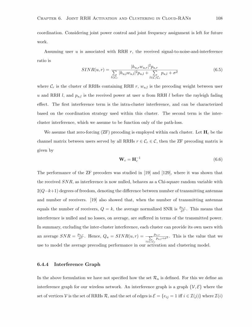
Chapter 6. Joint RRH Activation and Clustering in Cloud-RANs 108
coordination. Considering joint power control and joint frequency assignment is left for future
work.
Assuming user u is associated with RRH r, the received signal-to-noise-and-interference
ratio is
SINR(u, r) =|hu,rwu,r|2pu,r∑
l∈Cr|hu,lwu,l|2pu,l +
∑l∈C/Cr
pu,l + σ2(6.5)
where Cr is the cluster of RRHs containing RRH r, wu,l is the precoding weight between user
u and RRH l, and pu,l is the received power at user u from RRH l before the rayleigh fading
effect. The first interference term is the intra-cluster interference, and can be characterized
based on the coordination strategy used within this cluster. The second term is the inter-
cluster interference, which we assume to be function only of the path-loss.
We assume that zero-forcing (ZF) precoding is employed within each cluster. Let Hc be the
channel matrix between users served by all RRHs r ∈ Cr ∈ C, then the ZF precoding matrix is
given by
Wc = H−1c (6.6)
The performance of the ZF precoders was studied in [19] and [129], where it was shown that
the received SNR, as interference is now nulled, behaves as a Chi-square random variable with
2(Q−k+1) degrees of freedom, denoting the difference between number of transmitting antennas
and number of receivers. [19] also showed that, when the number of transmitting antennas
equals the number of receivers, Q = k, the average normalized SNR ispu,rσ2 . This means that
interference is nulled and no losses, on average, are suffered in terms of the transmitted power.
In summary, excluding the inter-cluster interference, each cluster can provide its own users with
an average SNR =pu,rσ2 . Hence, Qu = SINR(u, r) =
pu,r∑l∈C/Cr
pu,l+σ2 . This is the value that we
use to model the average precoding performance in our activation and clustering model.
6.4.4 Interference Graph
In the above formulation we have not specified how the set Ru is defined. For this we define an
interference graph for our wireless network. An interference graph is a graph {V, E} where the
set of vertices V is the set of RRHsR, and the set of edges is E = {eij = 1 iff i ∈ I(j)} where I(i)
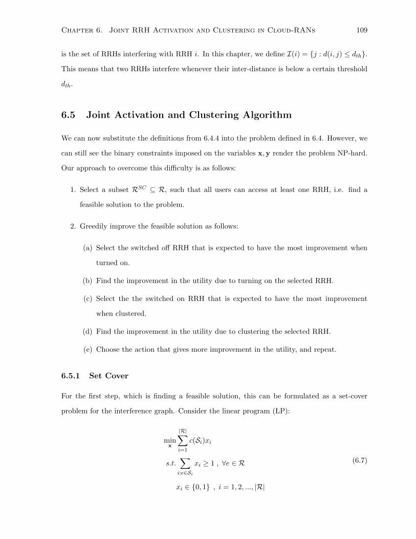
Chapter 6. Joint RRH Activation and Clustering in Cloud-RANs 109
is the set of RRHs interfering with RRH i. In this chapter, we define I(i) = {j : d(i, j) ≤ dth}.
This means that two RRHs interfere whenever their inter-distance is below a certain threshold
dth.
6.5 Joint Activation and Clustering Algorithm
We can now substitute the definitions from 6.4.4 into the problem defined in 6.4. However, we
can still see the binary constraints imposed on the variables x,y render the problem NP-hard.
Our approach to overcome this difficulty is as follows:
1. Select a subset RSC ⊆ R, such that all users can access at least one RRH, i.e. find a
feasible solution to the problem.
2. Greedily improve the feasible solution as follows:
(a) Select the switched off RRH that is expected to have the most improvement when
turned on.
(b) Find the improvement in the utility due to turning on the selected RRH.
(c) Select the the switched on RRH that is expected to have the most improvement
when clustered.
(d) Find the improvement in the utility due to clustering the selected RRH.
(e) Choose the action that gives more improvement in the utility, and repeat.
6.5.1 Set Cover
For the first step, which is finding a feasible solution, this can be formulated as a set-cover
problem for the interference graph. Consider the linear program (LP):
minx
|R|∑i=1
c(Si)xi
s.t.∑i:e∈Si
xi ≥ 1 , ∀e ∈ R
xi ∈ {0, 1} , i = 1, 2, ..., |R|
(6.7)
Chapter 6. Joint RRH Activation and Clustering in Cloud-RANs 110
where Si = Ii∪{i} is the set of cells covered by RRH i, which is also equal to the interference set
plus RRH i own cell. While the above problem is still NP-hard, it has an efficient approximation
scheme using linear-programming rounding. The first step is to solve a relaxed version of (6.7)
as follows:
minx
|R|∑i=1
c(Si)xi
s.t.∑i:e∈Si
xi ≥ 1 , ∀e ∈ R
0 ≤ xi ≤ 1 , i = 1, 2, ..., |R|
(6.8)
The output of problem (6.8) is then rounded to provide an integer solution using the
Algorithm summarized in Algorithm 6.1. This LP rounding scheme is known to be an f -
Algorithm 6.1 LP Rounding Set-Cover
1. Solve the relaxed version of the LP problem as shown in (6.8) to get x = (x1, x2, ..., x|R|);
2. Let f be the maximum frequency (the maximum number of times that an element appearsin distinct coverage sets);
3. Output deterministic rounding x = (x1, x2, ..., x|R|) ∈ {0, 1} where
xi =
{1 , xi ≥ 1/f
0 , otherwise
approximation of the set cover problem [143].
6.5.2 Greedy Improvement
The next step in our algorithm is to gradually improve upon the feasible solution found in
Algorithm 6.1. We follow a greedy approach, which can also be viewed as a discrete gradient
ascent one. The algorithm starts with the feasible solution found from Algorithm 6.1, and tries
to pick the direction that gives us the largest increase in the utility function. However, since
there are many decisions to choose from, activating each off RRH or clustering each pair of on
RRHs, we propose a simplification. First, we select the RRH that is most likely to improve
the utility. For the activation part, we pick the RRH which has the most users in its cell and
Chapter 6. Joint RRH Activation and Clustering in Cloud-RANs 111
is also turned off. While for the clustering part, we pick the RRH that is causing the most
interference. For each case, we find the utility improving by activation or clustering the chosen
RRH, and proceed with the one that gives us the larger improvement.
The steps are summarized in Algorithm 6.2. Step 1 finds the inactive RRH with the most
users within its cell. Step 3 finds the utility improvement resulting from activating this RRH.
Step 4 finds the active RRH that generates the most interference. Step 5 finds nearest interfering
RRH to the one selected in step 4. Step 7 finds the utility improvement from clustering the
two RRHs selected in steps 4 and 5. Finally the decision, either activation or clustering, with
the higher increase in utility is chosen in step 8. The process repeats until the marginal gain is
below a specified threshold or a maximum number of iterations is reached.
Algorithm 6.2 Greedy Improvement
• Do for n = 0→ N and 4xf,4yf > ε
1. Find i such that xi = 0 and Ui > Uj ∀j : xj = 0
2. Set xn+1 = xn ∀j 6= i and xn+1,i = 1
3. Find 4xf = f(xn+1, yn)− f(xn, yn)
4. Find k such that xk = 1 and∑
u∈U I(u, k) >∑
u∈U I(u, j) ∀j : xj = 1 and j /∈ Ck5. Find j such that d(k, j) < d(k, l) ∀l : xl = 1 and j, l /∈ Ck6. Set yn+1 = yn ∀v, w 6= i, j and yn+1,i,j = 1
7. Find 4yf = f(xn, yn+1)− f(xn, yn)
8.
xn+1, yn+1 =
{{xn+1, yn if 4xf ≥ 4yf
xn, yn+1 if 4yf < 4yf
6.6 Simulation Results
In this section we present performance results of the proposed solution to the optimization
problem. We simulate a network of 20 RRHs, distributed uniformly within an area of 39250m2,
where on average each AP has a cell of diameter 50 meters.
The main parameters that we vary in our simulations are dth and |U|. The first is the
interference threshold, whose higher values indicate a larger number of RRHs are needed to
provide coverage, and consequently being selected by the algorithm. In such case the greedy
Chapter 6. Joint RRH Activation and Clustering in Cloud-RANs 112
algorithm will favor clustering the already active RRHs over turning on new ones. The second
parameter is the average number of users. We vary this parameter from 1 user to 200 users per
RRH. This significantly affects the QoS performance, which will also be reflected in the greedy
algorithm decisions.
In Fig. 6.2 we show the average number of active RRHs as the the total number of users is
increased. First, we can see how the interference threshold throttles the domain of the greedy
algorithm. When the threshold is low, the number of RRHs selected by the set-cover problem
is already large, leaving little room for improvement in this side. As the interference threshold
reaches a value of 50, which is the average value of RRH inter-distance in our simulation, the
process saturates. We can already the significant energy savings available, this is particularly
important when the number of users is small. In such a case, almost half of all RRHs can be
turned off.
In Figures 6.3, 6.4 and 6.5 we study the behavior of the different components of QoS. The
main point here is to show how much improvement can be achieved by joint design of RRH
clustering and activation, hence confirming the benefit of our approach. Fig. 6.3 shows the
behavior of the first component of QoS (SIR) versus the total number of users. We can observe
up to 25% improvement in SIR QoS. Fig. 6.4 is beneficial to understanding the behavior of the
algorithm. It shows the QoS provided by the algorithm versus the number of RRHs activated
by it. We note that different lines start at different points due to the difference in the number
of initial RRHs activated by the set-cover problem. Fig. 6.5 shows the behavior of the overall
QoS, which is the weighted sum of SIR and the average number of users per RRH. The QoS
gains decrease when we consider the overall QoS. This confirms our rationale for studying both
PHY-layer and MAC-layer metrics.
In Fig. 6.6 and 6.7 we show the behavior of the algorithm as we change the area within
which the users and RRHs are co-located. We can see that for smaller areas, i.e. smaller density
factor, the number of active RRHs is less. This follows directly from the fact that once RRHs
are closer to each other, each RRH can cover more users. The interference threshold can be
tuned to control this behavior by forcing more RRHs to be turned on. In Fig. 6.7 we study
the behavior of QoS. We observe that as the density is increased, QoS is decreased. This is due
to the excessive clustering selected by the algorithm. As the RRHs become very far from each
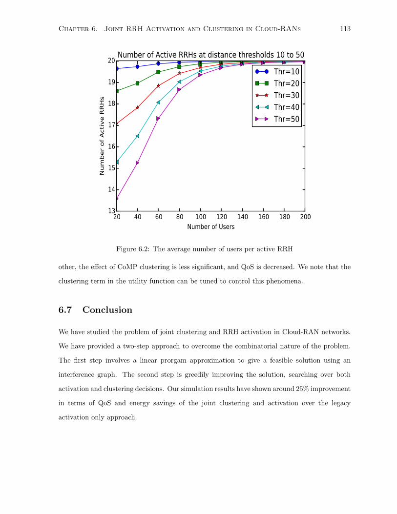
Chapter 6. Joint RRH Activation and Clustering in Cloud-RANs 113
20 40 60 80 100 120 140 160 180 200
Number of Users
13
14
15
16
17
18
19
20
Num
ber of Active R
RHs
Number of Active RRHs at distance thresholds 10 to 50
Thr=10
Thr=20
Thr=30
Thr=40
Thr=50
Figure 6.2: The average number of users per active RRH
other, the effect of CoMP clustering is less significant, and QoS is decreased. We note that the
clustering term in the utility function can be tuned to control this phenomena.
6.7 Conclusion
We have studied the problem of joint clustering and RRH activation in Cloud-RAN networks.
We have provided a two-step approach to overcome the combinatorial nature of the problem.
The first step involves a linear prorgam approximation to give a feasible solution using an
interference graph. The second step is greedily improving the solution, searching over both
activation and clustering decisions. Our simulation results have shown around 25% improvement
in terms of QoS and energy savings of the joint clustering and activation over the legacy
activation only approach.
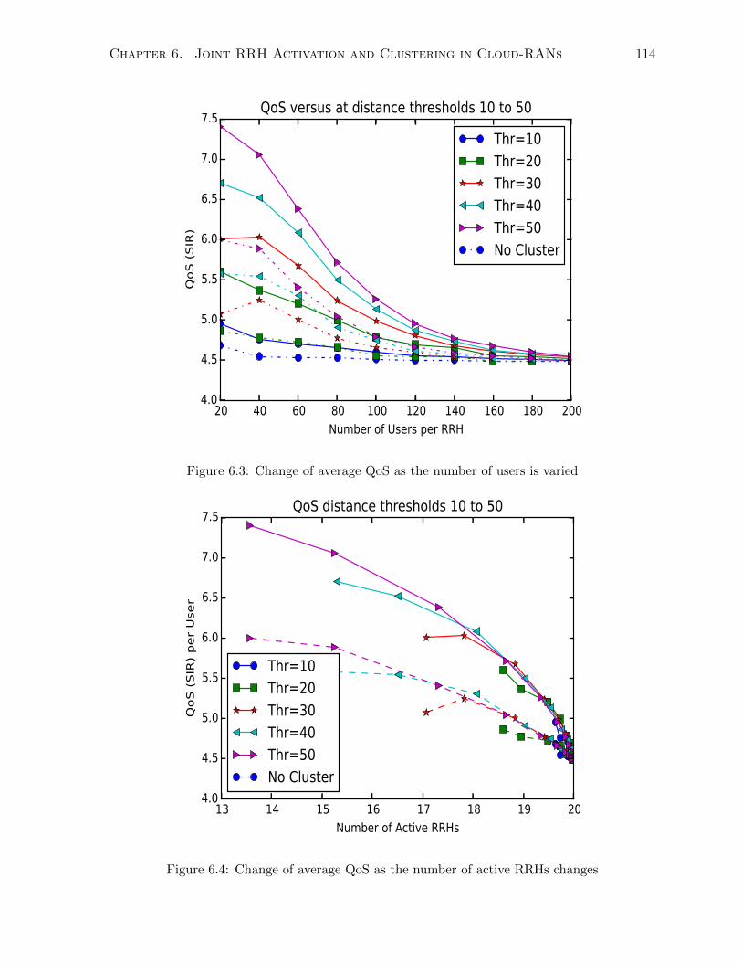
Chapter 6. Joint RRH Activation and Clustering in Cloud-RANs 114
20 40 60 80 100 120 140 160 180 200
Number of Users per RRH
4.0
4.5
5.0
5.5
6.0
6.5
7.0
7.5
QoS (SIR)
QoS versus at distance thresholds 10 to 50
Thr=10
Thr=20
Thr=30
Thr=40
Thr=50
No Cluster
Figure 6.3: Change of average QoS as the number of users is varied
13 14 15 16 17 18 19 20
Number of Active RRHs
4.0
4.5
5.0
5.5
6.0
6.5
7.0
7.5
Qo
S (
SIR
) p
er
Use
r
QoS distance thresholds 10 to 50
Thr=10
Thr=20
Thr=30
Thr=40
Thr=50
No Cluster
Figure 6.4: Change of average QoS as the number of active RRHs changes
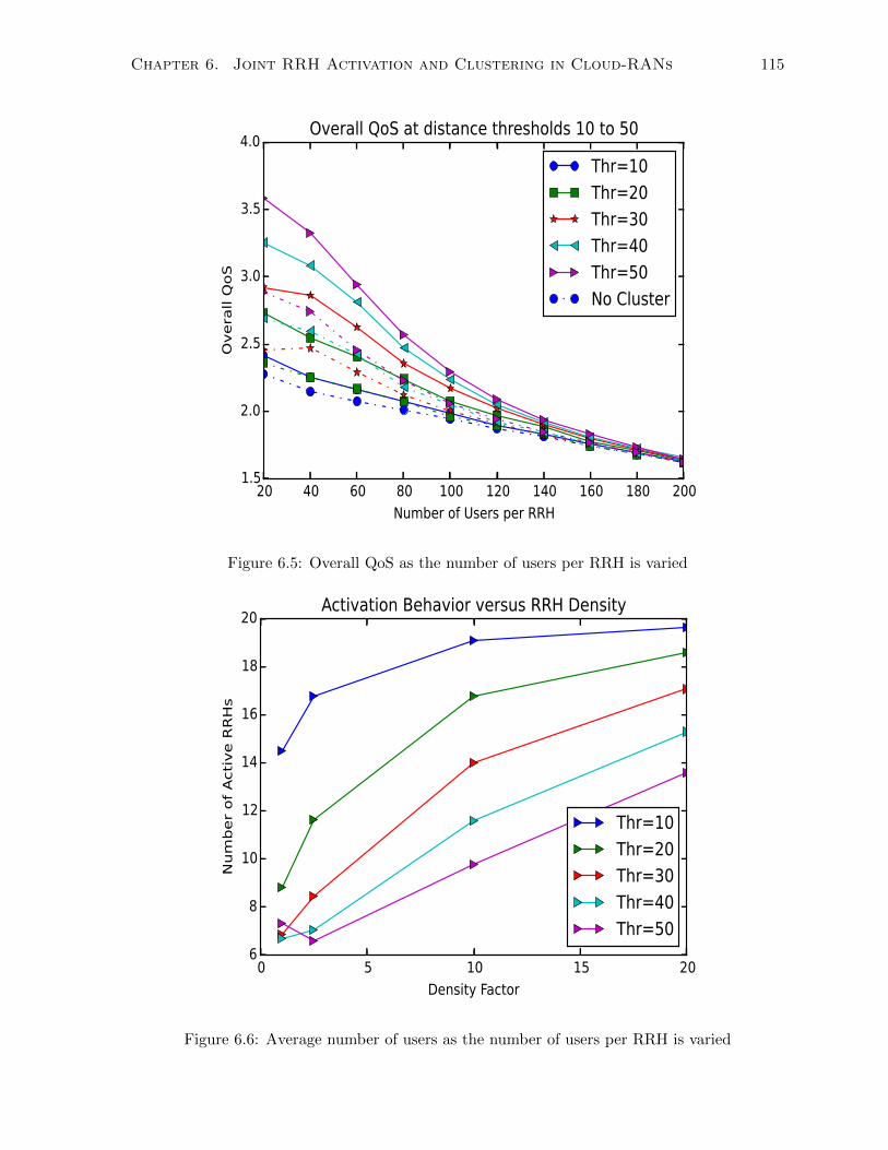
Chapter 6. Joint RRH Activation and Clustering in Cloud-RANs 115
20 40 60 80 100 120 140 160 180 200
Number of Users per RRH
1.5
2.0
2.5
3.0
3.5
4.0
Overall QoS
Overall QoS at distance thresholds 10 to 50
Thr=10
Thr=20
Thr=30
Thr=40
Thr=50
No Cluster
Figure 6.5: Overall QoS as the number of users per RRH is varied
0 5 10 15 20
Density Factor
6
8
10
12
14
16
18
20
Number of Active RRHs
Activation Behavior versus RRH Density
Thr=10
Thr=20
Thr=30
Thr=40
Thr=50
Figure 6.6: Average number of users as the number of users per RRH is varied
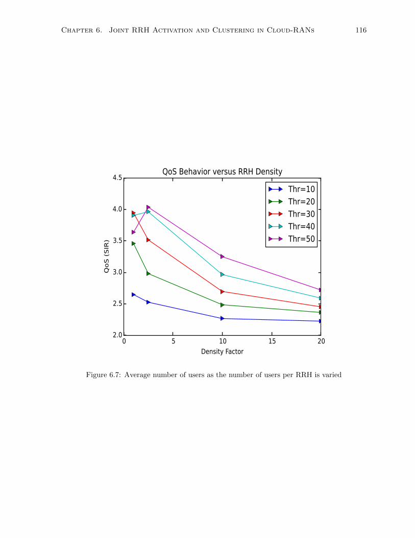
Chapter 6. Joint RRH Activation and Clustering in Cloud-RANs 116
0 5 10 15 20
Density Factor
2.0
2.5
3.0
3.5
4.0
4.5
QoS (SIR)
QoS Behavior versus RRH Density
Thr=10
Thr=20
Thr=30
Thr=40
Thr=50
Figure 6.7: Average number of users as the number of users per RRH is varied
Chapter 7
Long-term Activation, Clustering
and Association in Cloud-RAN
7.1 Context
In this chapter we build upon the work in Chapter 6 and extend it in several ways. While the
model used in the previous chapter showed the strong benefit of the joint activation-clustering
approach, there were two main aspects still missing. These are the dynamic and flexible user-
RRH association, and the temporal correlation of the user and traffic behavior, and consequently
the activation and clustering decisions. The more flexible association scheme we consider here
relieves us of having to always associate the user with its nearest RRH. Instead, users can be
dynamically hand-overed between the different RRHs, hence giving more flexibility to the acti-
vation and clustering decisions. In order to incorporate the temporal correlation, i.e. queuing,
into the model, we have to also include clustering as a variable and study its effect on the
SINR. We address these challenges by providing a comprehensive model that incorporates all
the aspects of activation, clustering and association. The resulting problem belongs to the class
of signomial optimization. We show how this problem can be efficiently solved using succes-
sive geometric approximation. Finally, we study how this approach can be extended into a
stochastic control one. The main idea is to perform the optimization based on the traffic fore-
cast. We measure the sensitivity of the activation and clustering decisions with respect to the
117
Chapter 7. Long-term Activation, Clustering and Association in Cloud-RAN118
forecast error, and find the error to be 9% and 18% for the activation and clustering decisions
respectively.
7.2 Introduction
The past few years have witnessed a large increase in cellular network traffic. Since the systems
are already operating close to their maximum capacity, one solution is to build more dense
wireless networks with aggressive frequency re-use factors. A dense network of RRHs ensures
less attenuation at the receiver side. However, two drawbacks are associated with these dense
networks: the first is the high energy consumption associated with such a large number of RRHs;
the second is the increased interference experienced by the receiver due to close proximity of
the transmitters.
In this Chapter, we study the same question as in the last chapter about energy-efficient
activation of RRHs. Previously, we studied the joint optimization of activation and clustering
and demonstrated the significant effect clustering has on the problem. Our goal now is to
extend the problem in two important ways:
• Association: User association is another aspect of the problem. Contrary to the tradi-
tional distance-based association, the high density of RRHs in cloud-RAN enables more
dynamic association schemes. Since the RRHs are closer to each other, instead of asso-
ciating a user to its nearest base station, it can instead be associated with one or more
nearby RRHs which can provide the user with comparable level of service but at a much
more balanced load. Eventually, even though the new RRH might be further from the
user, the low load on this RRH will help the user get more frequency resources to account
for the decrease in the received signal power.
• Queuing: The other major aspect is the strong time-dependency of the network load.
A decision to activate or de-activate a RRH will have a strong impact on the queues
occupancy and the network state at the next time slot. This strong temporal correlation
means that consecutive activation, clustering and association decisions are strongly inter-
twined, and should ideally be jointly optimized. This leads us to formulate the problem
Chapter 7. Long-term Activation, Clustering and Association in Cloud-RAN119
as a long-term optimization, where the queuing aspects are included to represent of the
temporal correlation of the state, and consequently the decisions.
In Fig. 7.1 we show the system architecture under study in this chapter. This is very
similar to the one in Chapter 6, except for the inclusion of association decisions as well. The
infrastructure controller communicates with the user process in order to find out about the
user’s position and its queue occupancy. This information is then used to decide upon the
activation and clustering of the RRHs as well as the association between the user and RRHs.
The activation decisions are then sent to the access network to activate/de-activate the corre-
sponding RRHs, while the clustering decisions are sent to the appropriate cell processes, and
the association decisions are sent to their respective users and cells processes.
7.3 Related Work
Besides the works reviewed in the previous chapter such as [133][108][55][104][132][131][163],
there is one more specific work that we would like to discuss here. The problem of dynamic base
station activation and user association was studied in [9]. This work has a lot of similarities with
ours, in that both study long-term optimization of RRH activation jointly with user association.
However, there are a few drawbacks with that approach that we intend to alleviate here:
• First and foremost clustering is not included in the model used in [9]. One of our main
contributions in this chapter is arriving at a generic form for SINR that integrates the
effect of RRH clustering for both interference coordination and joint transmission scenar-
ios. This form is necessary to be able to perform long-term optimization of the activation
and clustering decisions, since the traditional greedy approach to clustering might prove
infeasible once we go beyond a single time slot decision.
• The approach in [9] reduces to a form of greedy optimization that solves an optimization
problem for each time slot based on the current queue occupancy. Our approach solves
the whole problem at once, and utilizes traffic forecasts for the future decisions. Greedy
optimization based only on the current state ignores the typical cyclo-stationary pattern
of the user behavior and network traffic. In other words, the decision process for the
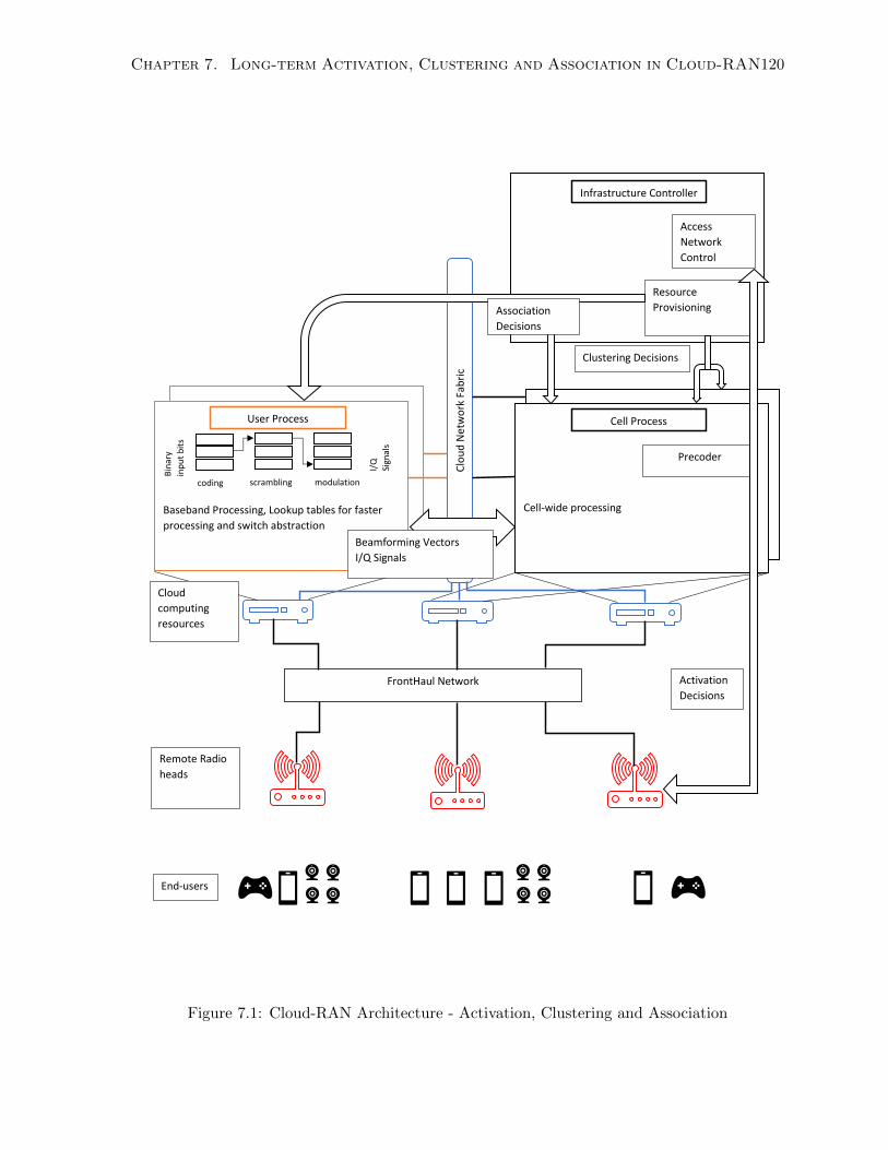
Chapter 7. Long-term Activation, Clustering and Association in Cloud-RAN120
Baseband Processing, Lookup tables for faster
processing and switch abstraction
Baseband Processing, Lookup tables for faster
processing and switch abstraction
Baseband Processing, Lookup tables for faster
processing and switch abstraction
FrontHaul Network
coding scrambling modulation
Bin
ary
inp
ut
bit
s
I/Q
Sign
als
Cloud
computing
resources
Remote Radio
heads
Cell-wide processing
User Process Cell Process
Precoder
Infrastructure Controller
Resource
Provisioning
Clo
ud
Net
wo
rk F
abri
c
Clustering Decisions
Access
Network
Control
Activation
Decisions
Beamforming Vectors
I/Q Signals
End-users
Association
Decisions
Figure 7.1: Cloud-RAN Architecture - Activation, Clustering and Association
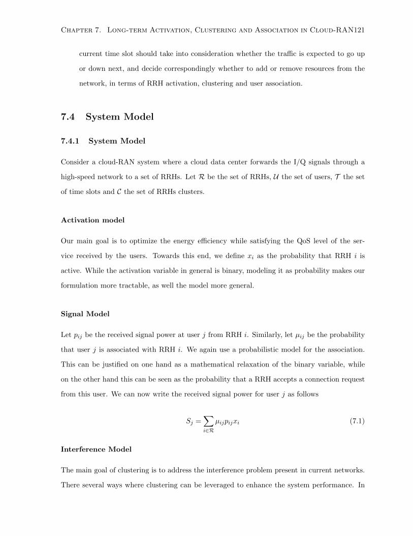
Chapter 7. Long-term Activation, Clustering and Association in Cloud-RAN121
current time slot should take into consideration whether the traffic is expected to go up
or down next, and decide correspondingly whether to add or remove resources from the
network, in terms of RRH activation, clustering and user association.
7.4 System Model
7.4.1 System Model
Consider a cloud-RAN system where a cloud data center forwards the I/Q signals through a
high-speed network to a set of RRHs. Let R be the set of RRHs, U the set of users, T the set
of time slots and C the set of RRHs clusters.
Activation model
Our main goal is to optimize the energy efficiency while satisfying the QoS level of the ser-
vice received by the users. Towards this end, we define xi as the probability that RRH i is
active. While the activation variable in general is binary, modeling it as probability makes our
formulation more tractable, as well the model more general.
Signal Model
Let pij be the received signal power at user j from RRH i. Similarly, let µij be the probability
that user j is associated with RRH i. We again use a probabilistic model for the association.
This can be justified on one hand as a mathematical relaxation of the binary variable, while
on the other hand this can be seen as the probability that a RRH accepts a connection request
from this user. We can now write the received signal power for user j as follows
Sj =∑i∈R
µijpijxi (7.1)
Interference Model
The main goal of clustering is to address the interference problem present in current networks.
There several ways where clustering can be leveraged to enhance the system performance. In
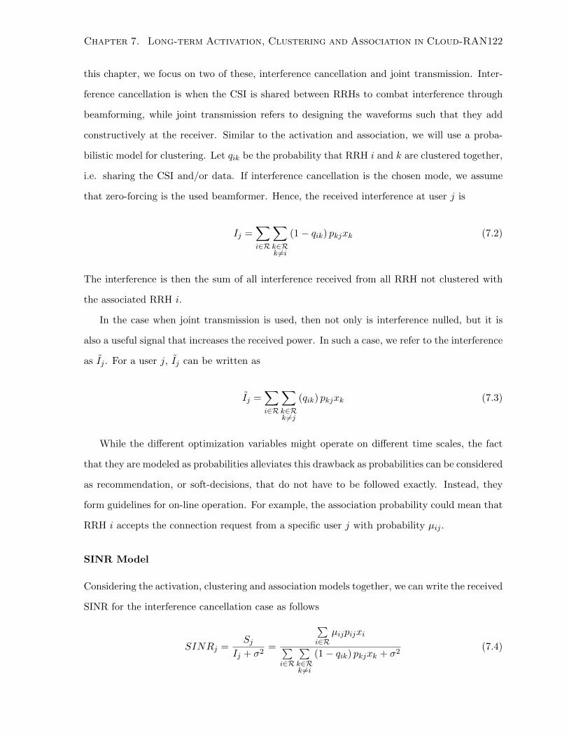
Chapter 7. Long-term Activation, Clustering and Association in Cloud-RAN122
this chapter, we focus on two of these, interference cancellation and joint transmission. Inter-
ference cancellation is when the CSI is shared between RRHs to combat interference through
beamforming, while joint transmission refers to designing the waveforms such that they add
constructively at the receiver. Similar to the activation and association, we will use a proba-
bilistic model for clustering. Let qik be the probability that RRH i and k are clustered together,
i.e. sharing the CSI and/or data. If interference cancellation is the chosen mode, we assume
that zero-forcing is the used beamformer. Hence, the received interference at user j is
Ij =∑i∈R
∑k∈Rk 6=i
(1− qik) pkjxk (7.2)
The interference is then the sum of all interference received from all RRH not clustered with
the associated RRH i.
In the case when joint transmission is used, then not only is interference nulled, but it is
also a useful signal that increases the received power. In such a case, we refer to the interference
as Ij . For a user j, Ij can be written as
Ij =∑i∈R
∑k∈Rk 6=j
(qik) pkjxk (7.3)
While the different optimization variables might operate on different time scales, the fact
that they are modeled as probabilities alleviates this drawback as probabilities can be considered
as recommendation, or soft-decisions, that do not have to be followed exactly. Instead, they
form guidelines for on-line operation. For example, the association probability could mean that
RRH i accepts the connection request from a specific user j with probability µij .
SINR Model
Considering the activation, clustering and association models together, we can write the received
SINR for the interference cancellation case as follows
SINRj =Sj
Ij + σ2=
∑i∈R
µijpijxi∑i∈R
∑k∈Rk 6=i
(1− qik) pkjxk + σ2(7.4)
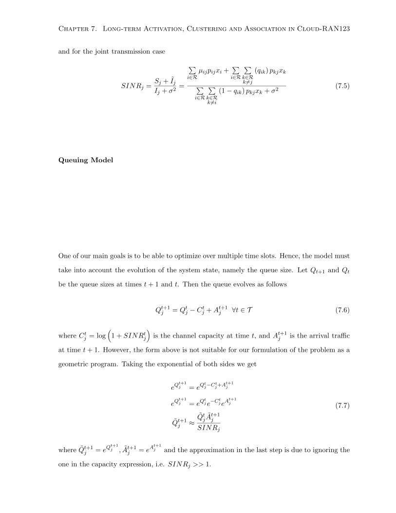
Chapter 7. Long-term Activation, Clustering and Association in Cloud-RAN123
and for the joint transmission case
SINRj =Sj + IjIj + σ2
=
∑i∈R
µijpijxi +∑i∈R
∑k∈Rk 6=j
(qik) pkjxk
∑i∈R
∑k∈Rk 6=i
(1− qik) pkjxk + σ2(7.5)
Queuing Model
One of our main goals is to be able to optimize over multiple time slots. Hence, the model must
take into account the evolution of the system state, namely the queue size. Let Qt+1 and Qt
be the queue sizes at times t+ 1 and t. Then the queue evolves as follows
Qt+1j = Qtj − Ctj +At+1
j ∀t ∈ T (7.6)
where Ctj = log(
1 + SINRtj
)is the channel capacity at time t, and At+1
j is the arrival traffic
at time t+ 1. However, the form above is not suitable for our formulation of the problem as a
geometric program. Taking the exponential of both sides we get
eQt+1j = eQ
tj−Ctj+A
t+1j
eQt+1j = eQ
tje−C
tjeA
t+1j
Qt+1j ≈
QtjAt+1j
SINRj
(7.7)
where Qt+1j = eQ
t+1j , At+1
j = eAt+1j and the approximation in the last step is due to ignoring the
one in the capacity expression, i.e. SINRj >> 1.
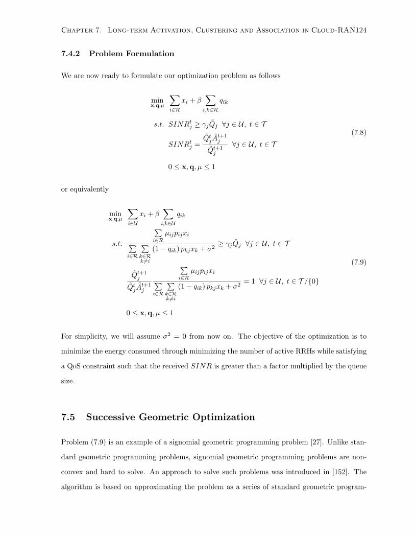
Chapter 7. Long-term Activation, Clustering and Association in Cloud-RAN124
7.4.2 Problem Formulation
We are now ready to formulate our optimization problem as follows
minx,q,µ
∑i∈R
xi + β∑i,k∈R
qik
s.t. SINRtj ≥ γjQj ∀j ∈ U , t ∈ T
SINRtj =QtjA
t+1j
Qt+1j
∀j ∈ U , t ∈ T
0 ≤ x,q, µ ≤ 1
(7.8)
or equivalently
minx,q,µ
∑i∈U
xi + β∑i,k∈U
qik
s.t.
∑i∈R
µijpijxi∑i∈R
∑k∈Rk 6=i
(1− qik) pkjxk + σ2≥ γjQj ∀j ∈ U , t ∈ T
Qt+1j
QtjAt+1j
∑i∈R
µijpijxi∑i∈R
∑k∈Rk 6=i
(1− qik) pkjxk + σ2= 1 ∀j ∈ U , t ∈ T /{0}
0 ≤ x,q, µ ≤ 1
(7.9)
For simplicity, we will assume σ2 = 0 from now on. The objective of the optimization is to
minimize the energy consumed through minimizing the number of active RRHs while satisfying
a QoS constraint such that the received SINR is greater than a factor multiplied by the queue
size.
7.5 Successive Geometric Optimization
Problem (7.9) is an example of a signomial geometric programming problem [27]. Unlike stan-
dard geometric programming problems, signomial geometric programming problems are non-
convex and hard to solve. An approach to solve such problems was introduced in [152]. The
algorithm is based on approximating the problem as a series of standard geometric program-
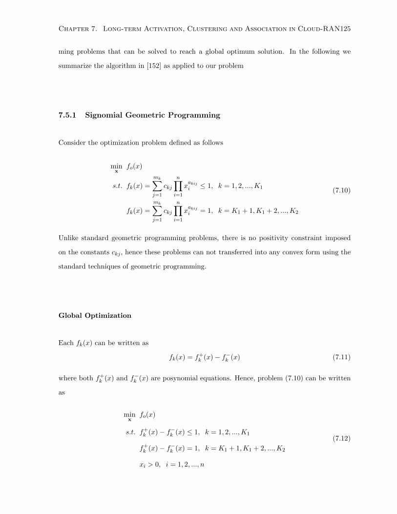
Chapter 7. Long-term Activation, Clustering and Association in Cloud-RAN125
ming problems that can be solved to reach a global optimum solution. In the following we
summarize the algorithm in [152] as applied to our problem
7.5.1 Signomial Geometric Programming
Consider the optimization problem defined as follows
minx
fo(x)
s.t. fk(x) =
mk∑j=1
ckj
n∏i=1
xakiji ≤ 1, k = 1, 2, ...,K1
fk(x) =
mk∑j=1
ckj
n∏i=1
xakiji = 1, k = K1 + 1,K1 + 2, ...,K2
(7.10)
Unlike standard geometric programming problems, there is no positivity constraint imposed
on the constants ckj , hence these problems can not transferred into any convex form using the
standard techniques of geometric programming.
Global Optimization
Each fk(x) can be written as
fk(x) = f+k (x)− f−k (x) (7.11)
where both f+k (x) and f−k (x) are posynomial equations. Hence, problem (7.10) can be written
as
minx
fo(x)
s.t. f+k (x)− f−k (x) ≤ 1, k = 1, 2, ...,K1
f+k (x)− f−k (x) = 1, k = K1 + 1,K1 + 2, ...,K2
xi > 0, i = 1, 2, ..., n
(7.12)
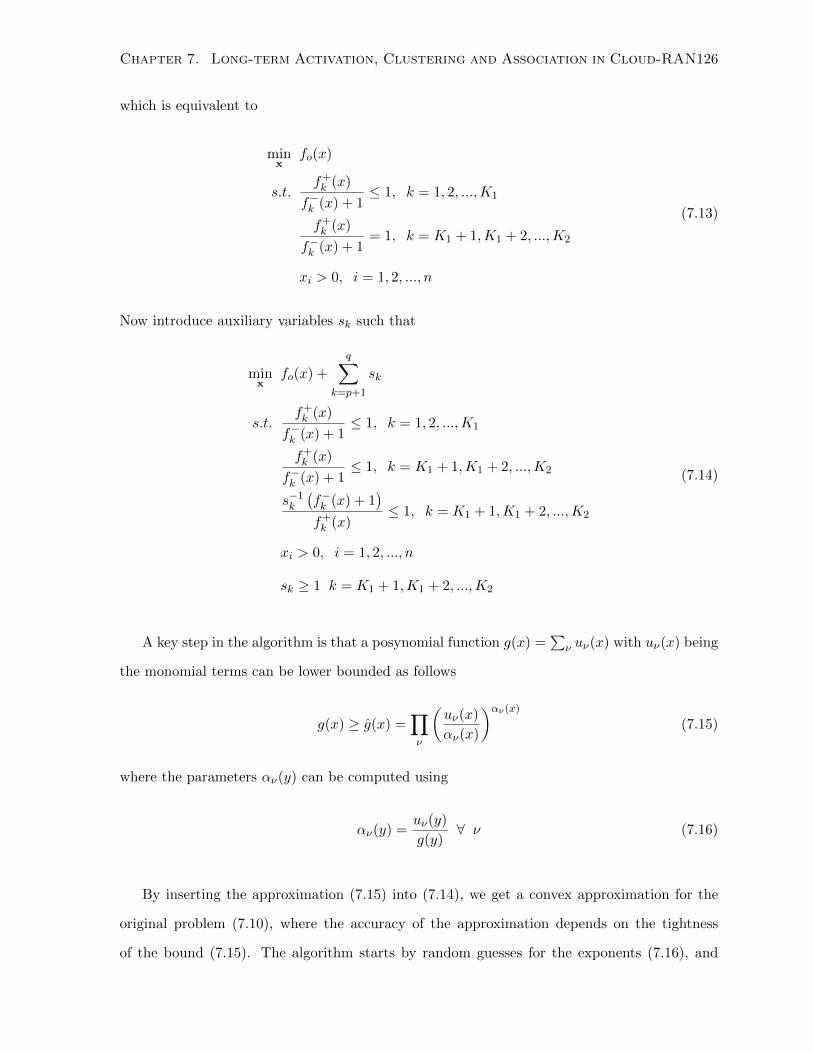
Chapter 7. Long-term Activation, Clustering and Association in Cloud-RAN126
which is equivalent to
minx
fo(x)
s.t.f+k (x)
f−k (x) + 1≤ 1, k = 1, 2, ...,K1
f+k (x)
f−k (x) + 1= 1, k = K1 + 1,K1 + 2, ...,K2
xi > 0, i = 1, 2, ..., n
(7.13)
Now introduce auxiliary variables sk such that
minx
fo(x) +
q∑k=p+1
sk
s.t.f+k (x)
f−k (x) + 1≤ 1, k = 1, 2, ...,K1
f+k (x)
f−k (x) + 1≤ 1, k = K1 + 1,K1 + 2, ...,K2
s−1k(f−k (x) + 1
)f+k (x)
≤ 1, k = K1 + 1,K1 + 2, ...,K2
xi > 0, i = 1, 2, ..., n
sk ≥ 1 k = K1 + 1,K1 + 2, ...,K2
(7.14)
A key step in the algorithm is that a posynomial function g(x) =∑
ν uν(x) with uν(x) being
the monomial terms can be lower bounded as follows
g(x) ≥ g(x) =∏ν
(uν(x)
αν(x)
)αν(x)(7.15)
where the parameters αν(y) can be computed using
αν(y) =uν(y)
g(y)∀ ν (7.16)
By inserting the approximation (7.15) into (7.14), we get a convex approximation for the
original problem (7.10), where the accuracy of the approximation depends on the tightness
of the bound (7.15). The algorithm starts by random guesses for the exponents (7.16), and
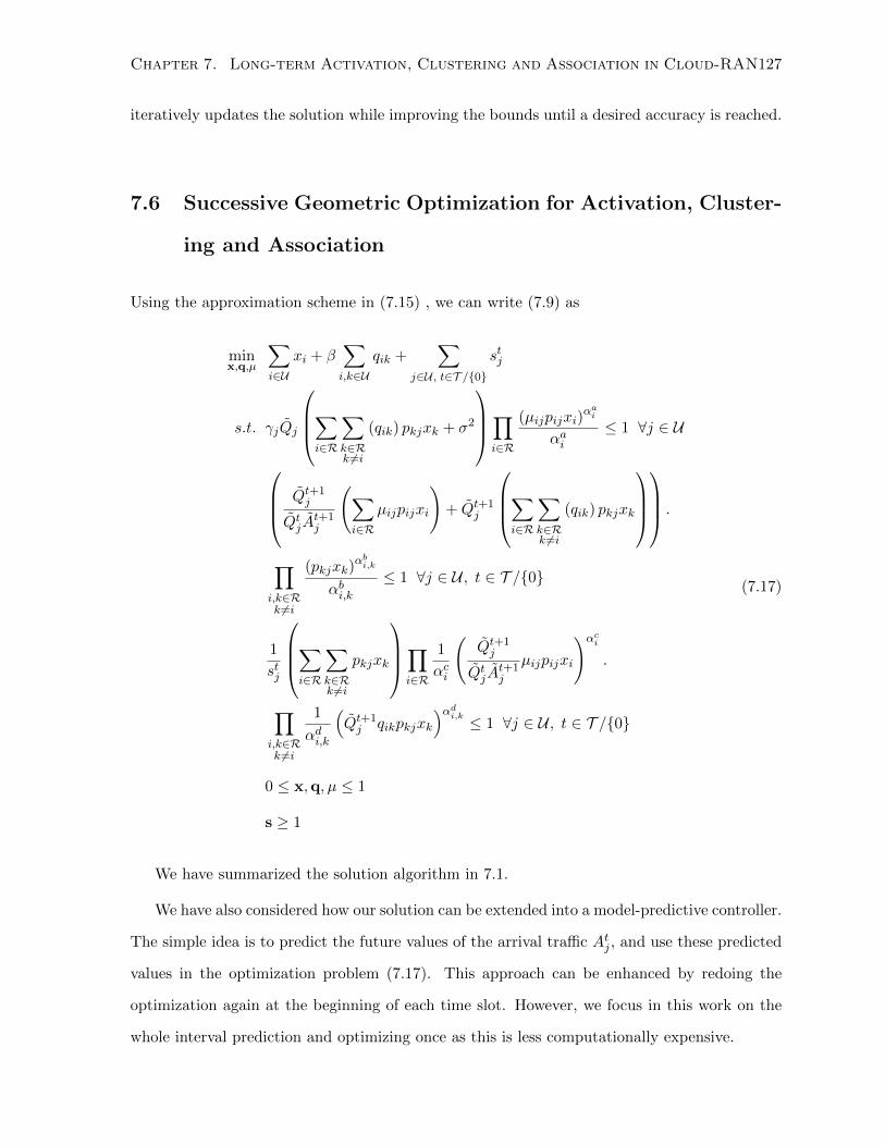
Chapter 7. Long-term Activation, Clustering and Association in Cloud-RAN127
iteratively updates the solution while improving the bounds until a desired accuracy is reached.
7.6 Successive Geometric Optimization for Activation, Cluster-
ing and Association
Using the approximation scheme in (7.15) , we can write (7.9) as
minx,q,µ
∑i∈U
xi + β∑i,k∈U
qik +∑
j∈U , t∈T /{0}
stj
s.t. γjQj
∑i∈R
∑k∈Rk 6=i
(qik) pkjxk + σ2
∏i∈R
(µijpijxi)αai
αai≤ 1 ∀j ∈ U
Qt+1j
QtjAt+1j
(∑i∈R
µijpijxi
)+ Qt+1
j
∑i∈R
∑k∈Rk 6=i
(qik) pkjxk
.
∏i,k∈Rk 6=i
(pkjxk)αbi,k
αbi,k≤ 1 ∀j ∈ U , t ∈ T /{0}
1
stj
∑i∈R
∑k∈Rk 6=i
pkjxk
∏i∈R
1
αci
(Qt+1j
QtjAt+1j
µijpijxi
)αci.
∏i,k∈Rk 6=i
1
αdi,k
(Qt+1j qikpkjxk
)αdi,k ≤ 1 ∀j ∈ U , t ∈ T /{0}
0 ≤ x,q, µ ≤ 1
s ≥ 1
(7.17)
We have summarized the solution algorithm in 7.1.
We have also considered how our solution can be extended into a model-predictive controller.
The simple idea is to predict the future values of the arrival traffic Atj , and use these predicted
values in the optimization problem (7.17). This approach can be enhanced by redoing the
optimization again at the beginning of each time slot. However, we focus in this work on the
whole interval prediction and optimizing once as this is less computationally expensive.
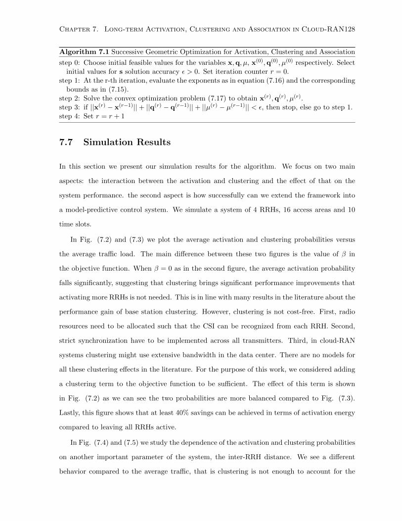
Chapter 7. Long-term Activation, Clustering and Association in Cloud-RAN128
Algorithm 7.1 Successive Geometric Optimization for Activation, Clustering and Association
step 0: Choose initial feasible values for the variables x,q, µ, x(0),q(0), µ(0) respectively. Selectinitial values for s solution accuracy ε > 0. Set iteration counter r = 0.
step 1: At the r-th iteration, evaluate the exponents as in equation (7.16) and the correspondingbounds as in (7.15).
step 2: Solve the convex optimization problem (7.17) to obtain x(r),q(r), µ(r).step 3: if ||x(r) − x(r−1)||+ ||q(r) − q(r−1)||+ ||µ(r) − µ(r−1)|| < ε, then stop, else go to step 1.step 4: Set r = r + 1
7.7 Simulation Results
In this section we present our simulation results for the algorithm. We focus on two main
aspects: the interaction between the activation and clustering and the effect of that on the
system performance. the second aspect is how successfully can we extend the framework into
a model-predictive control system. We simulate a system of 4 RRHs, 16 access areas and 10
time slots.
In Fig. (7.2) and (7.3) we plot the average activation and clustering probabilities versus
the average traffic load. The main difference between these two figures is the value of β in
the objective function. When β = 0 as in the second figure, the average activation probability
falls significantly, suggesting that clustering brings significant performance improvements that
activating more RRHs is not needed. This is in line with many results in the literature about the
performance gain of base station clustering. However, clustering is not cost-free. First, radio
resources need to be allocated such that the CSI can be recognized from each RRH. Second,
strict synchronization have to be implemented across all transmitters. Third, in cloud-RAN
systems clustering might use extensive bandwidth in the data center. There are no models for
all these clustering effects in the literature. For the purpose of this work, we considered adding
a clustering term to the objective function to be sufficient. The effect of this term is shown
in Fig. (7.2) as we can see the two probabilities are more balanced compared to Fig. (7.3).
Lastly, this figure shows that at least 40% savings can be achieved in terms of activation energy
compared to leaving all RRHs active.
In Fig. (7.4) and (7.5) we study the dependence of the activation and clustering probabilities
on another important parameter of the system, the inter-RRH distance. We see a different
behavior compared to the average traffic, that is clustering is not enough to account for the
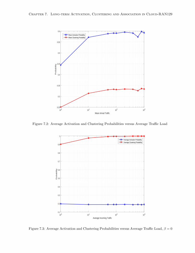
Chapter 7. Long-term Activation, Clustering and Association in Cloud-RAN129
100 101 102 103
Mean Arrival Traffic
0.25
0.3
0.35
0.4
0.45
0.5
0.55
0.6
Pro
ba
bility
Mean Activation ProbabilityMean Clustering Probability
Figure 7.2: Average Activation and Clustering Probabilities versus Average Traffic Load
100 101 102 103
Average Incoming Traffic
0.1
0.2
0.3
0.4
0.5
0.6
0.7
0.8
0.9
1
Pro
ba
bility
Average Activation ProbabilityAverage Clustering Probability
Figure 7.3: Average Activation and Clustering Probabilities versus Average Traffic Load, β = 0
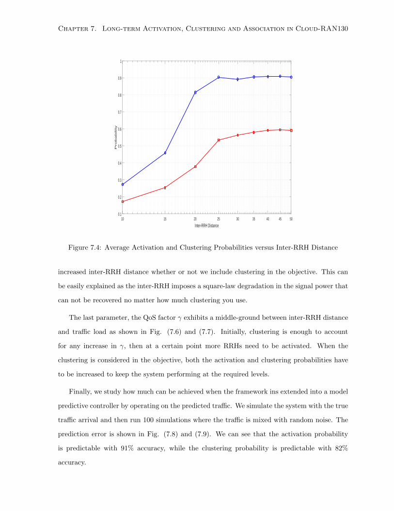
Chapter 7. Long-term Activation, Clustering and Association in Cloud-RAN130
10 15 20 25 30 35 40 45 50
Inter-RRH Distance
0.1
0.2
0.3
0.4
0.5
0.6
0.7
0.8
0.9
1
Probability
Figure 7.4: Average Activation and Clustering Probabilities versus Inter-RRH Distance
increased inter-RRH distance whether or not we include clustering in the objective. This can
be easily explained as the inter-RRH imposes a square-law degradation in the signal power that
can not be recovered no matter how much clustering you use.
The last parameter, the QoS factor γ exhibits a middle-ground between inter-RRH distance
and traffic load as shown in Fig. (7.6) and (7.7). Initially, clustering is enough to account
for any increase in γ, then at a certain point more RRHs need to be activated. When the
clustering is considered in the objective, both the activation and clustering probabilities have
to be increased to keep the system performing at the required levels.
Finally, we study how much can be achieved when the framework ins extended into a model
predictive controller by operating on the predicted traffic. We simulate the system with the true
traffic arrival and then run 100 simulations where the traffic is mixed with random noise. The
prediction error is shown in Fig. (7.8) and (7.9). We can see that the activation probability
is predictable with 91% accuracy, while the clustering probability is predictable with 82%
accuracy.
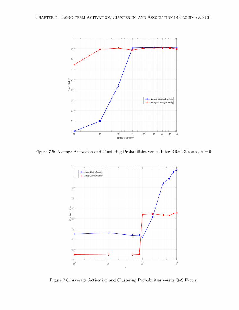
Chapter 7. Long-term Activation, Clustering and Association in Cloud-RAN131
10 15 20 25 30 35 40 45 50
Inter RRH distance
0.1
0.2
0.3
0.4
0.5
0.6
0.7
0.8
0.9
1
Pro
ba
bility
Average Activation ProbabilityAverage Clustering Probability
Figure 7.5: Average Activation and Clustering Probabilities versus Inter-RRH Distance, β = 0
100 101 102 103
γ
0.2
0.3
0.4
0.5
0.6
0.7
0.8
0.9
1
1.1
Probability
Average Activation ProbabilityAverage Clsutering Probability
Figure 7.6: Average Activation and Clustering Probabilities versus QoS Factor
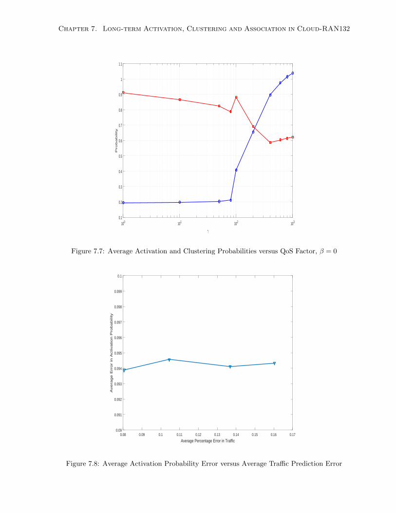
Chapter 7. Long-term Activation, Clustering and Association in Cloud-RAN132
100 101 102 103
γ
0.1
0.2
0.3
0.4
0.5
0.6
0.7
0.8
0.9
1
1.1
Probability
Figure 7.7: Average Activation and Clustering Probabilities versus QoS Factor, β = 0
0.08 0.09 0.1 0.11 0.12 0.13 0.14 0.15 0.16 0.17
Average Percentage Error in Traffic
0.09
0.091
0.092
0.093
0.094
0.095
0.096
0.097
0.098
0.099
0.1
Ave
rag
e E
rro
r in
Activa
tio
n P
rob
ab
ility
Figure 7.8: Average Activation Probability Error versus Average Traffic Prediction Error
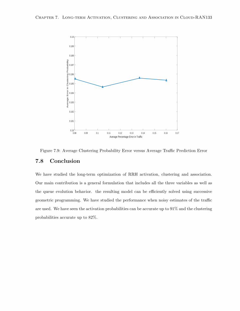
Chapter 7. Long-term Activation, Clustering and Association in Cloud-RAN133
0.08 0.09 0.1 0.11 0.12 0.13 0.14 0.15 0.16 0.17
Average Percentage Error in Traffic
0.18
0.181
0.182
0.183
0.184
0.185
0.186
0.187
0.188
0.189
0.19
Ave
rag
e E
rro
r in
Clu
ste
rin
g P
rob
ab
ility
Figure 7.9: Average Clustering Probability Error versus Average Traffic Prediction Error
7.8 Conclusion
We have studied the long-term optimization of RRH activation, clustering and association.
Our main contribution is a general formulation that includes all the three variables as well as
the queue evolution behavior. the resulting model can be efficiently solved using successive
geometric programming. We have studied the performance when noisy estimates of the traffic
are used. We have seen the activation probabilities can be accurate up to 91% and the clustering
probabilities accurate up to 82%.
Chapter 8
Graph-based Diagnosis in
Software-Defined Infrastructure
8.1 Context
In cloud-RAN systems, the infrastructure controller is responsible for the monitoring, diagno-
sis and dynamic scaling of cloud computing resources in order to provide resource elasticity.
The infrastructure controller needs to ensure the user/cell process has not been compromised
before assigning any extra resource. Hence, anomaly detection is the first step towards secure
resource management. However, investigating individual resource behavior may not be efficient
in detecting abnormal behavior in large and complex datacenters. In this chapter, we propose
a scalable graph based diagnosis framework to detect system anomalies in Software-Defined
Infrastructure running in the SAVI testbed. We have leveraged Graph Mining and Machine
Learning techniques in our approach in order to detect different kinds of anomalies. We have ex-
perimentally tested our framework on several use cases: Webserver-Database workload pattern,
bandwidth throttling between a pair of VMs, denial-of-service (DoS) attack on a webserver
and Spark Job failure. Our framework was able to detect all the aforementioned anomalies
accurately 1.
1This chapter is a joint work with Joseph Wahba, a former MSc student in our research group.
134
Chapter 8. Graph-based Diagnosis in Software-Defined Infrastructure 135
8.2 Introduction
In this chapter, and the next, we focus on the cloud computing aspect of the system. Particu-
larly, we study the anomaly detection and auto-scaling problems. The Cloud computing model
is increasingly being adopted in enterprises and service providers as it allows them to seam-
lessly manage their infrastructures. It was then natural to develop the next generation wireless
architecture, cloud-RAN, as a cloud-based architecture. Virtualization has become the en-
abler technology in today’s data centers. Through virtualization of networking and computing
resources, we can provide both infrastructure-as-a-service (IaaS), network-as-a-service (NaaS)
and platform-as-a-service (PaaS). These services enable sharing the infrastructure between dif-
ferent network slices. Hence, it is now possible to rapidly deploy applications on computing
infrastructure and speed up the rate of innovation.
As different cloud platforms continue to grow in scale and complexity (including C-RAN),
the diagnosis and management task of cloud data centers and platforms becomes a critical
challenge. Dynamic management of the cloud resources by upscaling/downscaling is at the
heart of the cloud economic model. A critical part of the resource management is detecting
abnormal behaviors in a data center in order to spot unusual system behaviors such as operator
errors, hardware, software failures, different attacks and anomalous communication patterns.
The cloud-focused architecture we envision for C-RAN is shown in Fig. 8.1. The controller
monitors the capacity of the physical and virtual machines on which the user process is running.
It also monitors the process itself in terms of computing resources both needed and assigned.
Once the infrastructure controller decides that the user process needs more computing resources,
it can either upgrade the underlying virtual machine, or migrate the whole process to a different
physical machine altogether. This decision by the infrastructure controller can be made based
on either the actual monitored state of the process, or the controller’s own prediction of the
process needs, as will be discussed in the next chapter. An important step before the scaling
decision is identifying whether the observed behavior is normal or anomalous. If the controller
suspects that virtual machine has been compromised, then it should be quarantined instead
of given extra resources. In this chapter we start by studying the anomaly detection problem,
and we study the joint anomaly detection and resource scaling in the next chapter. While we
Chapter 8. Graph-based Diagnosis in Software-Defined Infrastructure 136
have not actually implemented the wireless base-band processing of the user process, we have
designed the approaches in this chapter and the next to be as applicable as possible to the full
cloud-RAN case.
The anomaly detection process can be considered as a closed-loop system, involving data
collection, processing as well as decision making and execution. Resource based anomaly de-
tection techniques are useful in diagnosing anomalies in individual resources. By leveraging
Graph-Mining and Machine Learning techniques, unusual behaviors in data centers could be
detected not only based on a per-resource behavior, but using a holistic view of inter-dependency
and inter-communication pattern between different resources.
One example of a data center cloud management platform is the SAVI [71] testbed on
which we have implemented our approach. The SAVI project was established to investigate
future application platforms designed for rapid applications deployment. SAVI testbed has
been developed for controlling and managing converged virtual resources focused on computing
and networking. In a SAVI Smart Edge we have compute, network, storage, FPGA, and other
resources. OpenStack [1] is used for managing compute, storage, GPU and FPGA resources.
OpenFlow [91] controllers are used for controlling network resources such as switches.
Our main contribution in this chapter is developing a graph-based anomaly detection frame-
work for the SAVI testbed. Our framework leverages the Apache Spark big-data platform for
scalability. We have tested our framework on several use cases including Webserver-Database
workload pattern, bandwidth throttling between a pair of VMs, denial-of-service (DoS) attack
on a webserver and Spark Job failure. Our framework was able to detect the aforementioned
anomalies accurately.
8.3 Related Work
Graph based Anomaly detection has been studied under many different settings using various
statistics tools and graph mining algorithms [12]. There are two main categories of approaches
for detecting anomalies in graphs: Methods for static graph and approaches for dynamic graph
data.

Chapter 8. Graph-based Diagnosis in Software-Defined Infrastructure 137
Baseband Processing, Lookup tables for faster
processing and switch abstraction
Baseband Processing, Lookup tables for faster
processing and switch abstraction
FrontHaul Network
coding scrambling modulation
Bin
ary
inp
ut
bit
s
I/Q
Sign
als
Cloud
computing
resources
Remote Radio
heads
User Process
Infrastructure Controller
Computing
resources scaling
and migration
Clo
ud
Net
wo
rk F
abri
c
VM utilization
Scaling decisions
End-users
Figure 8.1: Cloud-RAN Architecture - Anomaly Detection and Scaling
Chapter 8. Graph-based Diagnosis in Software-Defined Infrastructure 138
8.3.1 Anomaly Detection in Static Graphs
In static graphs, the main task for anomaly detection is to discover anomalous network entities
(e.g., nodes, edges) given the entire graph structure. Static graphs are either plain graphs which
do not have attributes or attributed graphs where nodes and/or edges have features associated
with them. Given a snapshot of a plain or attributed graph, the anomaly detection problem
could be defined as finding the nodes and/or edges that are few and significantly different
from the patterns observed in the rest of the graph. In static plain graphs, the only available
information is the graph’s structure. Therefore, in order to detect anomalies, the structure
of the graph is used to find patterns and spot anomalies. There are two main categories of
methods in detecting anomalies in static plain graphs: structure-based methods [58] [26] [44]
[59] and community-based methods [134] [29] [140] [153]. In static attributed graphs, anomaly
detection methods exploit the structure as well as the correlation of attributes of the graph to
find patterns and spot anomalies [102] [40] [83]. In community based methods, approaches aim
to identify those outlier nodes in a graph whose attribute values deviate significantly from the
other members of the specific communities where they belong [47] [153] [98].
8.3.2 Anomaly Detection in Dynamic Graphs
Dynamic graphs are time-evolving graphs which are composed of sequences of static graphs.
Given a sequence of graphs, the anomaly detection problem could be defined as whether the
graph has become significantly different from its predecessors. Hence, it is necessary to de-
fine two things: first the features that represent a graph; second a distance measure between
these features. Based on the distance, we can train the system to decide whether a specific
graph is anomalous or not. The authors in [25] studied different graph similarity measures,
anomaly detection techniques in large network based data and clustering similar graphs to-
gether. Different approaches have been used in detecting anomalies in dynamic graphs such
as feature-based events [72] [121] [28], decomposition-based events [11] [117], clustering-based
[73] [99] and window-based events [110] [96]. In [66], an eigen-space based approach has been
proposed for modeling graphs and detecting anomalies.
In contrast to the current work, we focus on anomaly detection in the physical infrastruc-
Chapter 8. Graph-based Diagnosis in Software-Defined Infrastructure 139
ture itself, unlike [66], and detect a wider range of anomalies in several use cases. We have
used a novel approach in detecting anomalies by leveraging both graph-based metrics and ma-
chine learning techniques. Our work is the first to address graph-based anomaly detection in
virtualized heterogeneous environments.
8.3.3 Graph Centrality Measures
There has been extensive work on quantifying a graph from the perspectives of centrality,
robustness, criticality and connectivity. In [36], node connectivity has been chosen as the best
metric to quantify graph robustness. The authors of [35] have introduced the symmetry-ratio
as a measure of graph symmetry. The concept of network criticality has been discussed in
[138],[139] as another of graph robustness. Our interest in these metrics stems from the fact
that they can be used as efficient graph features in the detection of anomalies.
8.4 System Architecture
In this section of the chapter we present our system architecture used for graph-based diag-
nosis in the SAVI testbed. Figure 8.2 depicts the architecture for our system. The system
is composed of four main modules: The monitoring and measurements module, the diagnos-
tics module, the decision making module and the orchestration module. The monitoring and
measurements module is responsible for collecting different metrics from SAVI heterogeneous
resources such as Network and Compute metrics and building graphs for different applications
running in SAVI testbed. The diagnostics module is responsible for performing the Graph-based
Anomaly Detection which present in this chapter. The decision making module is responsible
for performing suitable actions in order to heal the system from the effect of the anomalies.
Finally, the orchestration module is responsible for executing the suitable decisions made in
order to return the system to its steady state condition. The focus of this chapter is on the
diagnostics module as this is where the anomaly detection is done.
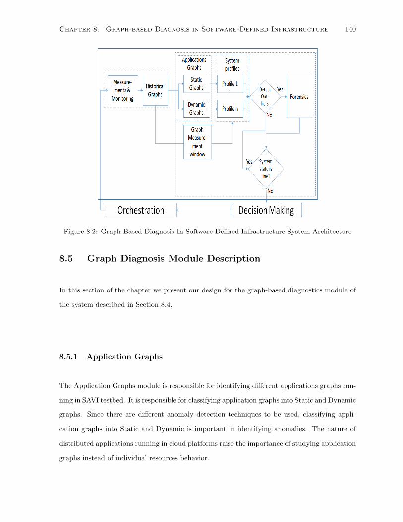
Chapter 8. Graph-based Diagnosis in Software-Defined Infrastructure 140
Figure 8.2: Graph-Based Diagnosis In Software-Defined Infrastructure System Architecture
8.5 Graph Diagnosis Module Description
In this section of the chapter we present our design for the graph-based diagnostics module of
the system described in Section 8.4.
8.5.1 Application Graphs
The Application Graphs module is responsible for identifying different applications graphs run-
ning in SAVI testbed. It is responsible for classifying application graphs into Static and Dynamic
graphs. Since there are different anomaly detection techniques to be used, classifying appli-
cation graphs into Static and Dynamic is important in identifying anomalies. The nature of
distributed applications running in cloud platforms raise the importance of studying application
graphs instead of individual resources behavior.
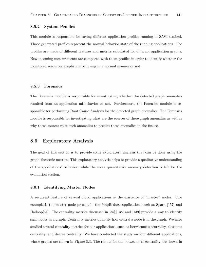
Chapter 8. Graph-based Diagnosis in Software-Defined Infrastructure 141
8.5.2 System Profiles
This module is responsible for saving different application profiles running in SAVI testbed.
Those generated profiles represent the normal behavior state of the running applications. The
profiles are made of different features and metrics calculated for different application graphs.
New incoming measurements are compared with those profiles in order to identify whether the
monitored resources graphs are behaving in a normal manner or not.
8.5.3 Forensics
The Forensics module is responsible for investigating whether the detected graph anomalies
resulted from an application misbehavior or not. Furthermore, the Forensics module is re-
sponsible for performing Root Cause Analysis for the detected graph anomalies. The Forensics
module is responsible for investigating what are the sources of these graph anomalies as well as
why these sources raise such anomalies to predict these anomalies in the future.
8.6 Exploratory Analysis
The goal of this section is to provide some exploratory analysis that can be done using the
graph-theoretic metrics. This exploratory analysis helps to provide a qualitative understanding
of the applications’ behavior, while the more quantitative anomaly detection is left for the
evaluation section.
8.6.1 Identifying Master Nodes
A recurrent feature of several cloud applications is the existence of ”master” nodes. One
example is the master node present in the MapReduce applications such as Spark [157] and
Hadoop[54]. The centrality metrics discussed in [35],[138] and [139] provide a way to identify
such nodes in a graph. Centrality metrics quantify how central a node is in the graph. We have
studied several centrality metrics for our applications, such as betweenness centrality, closeness
centrality, and degree centrality. We have conducted the study on four different applications,
whose graphs are shown in Figure 8.3. The results for the betweenness centrality are shown in
Chapter 8. Graph-based Diagnosis in Software-Defined Infrastructure 142
Figure 8.3: Graphs of Different Applications
Figure 8.4 and Figure 8.5.
It can be observed that the larger difference between the maximum and average betweenness
for a specific graph matches the existence of a central node as shown in Figure 8.3. For example,
application 4 exhibits the largest difference between the mean and maximum centrality. We can
see that for application 4, the graph is composed of a central node holding three other nodes
together. Next one is application 3, which has pseudo-central node holding the graph together,
but some other nodes have their connectivity outside this central node. Last is application 1,
which has an almost mesh-like graph, resulting in small values for the maximum centrality.
8.6.2 Assortativity
Another metric is Assortativity. Assortativity measures the correlation between the degrees
of the connected nodes. A graph is assortative if its high degree nodes are connected to high
degree nodes, and low degree nodes are connected to low degree nodes, in which case it will
have a more positive assortativity coefficient. We can see in Figure 8.6 that application 1 has
the highest assortativity due to the almost uniform connectivity of its nodes. On the other
hand, application 4 has the lowest assortativity. The presence of a central node in application
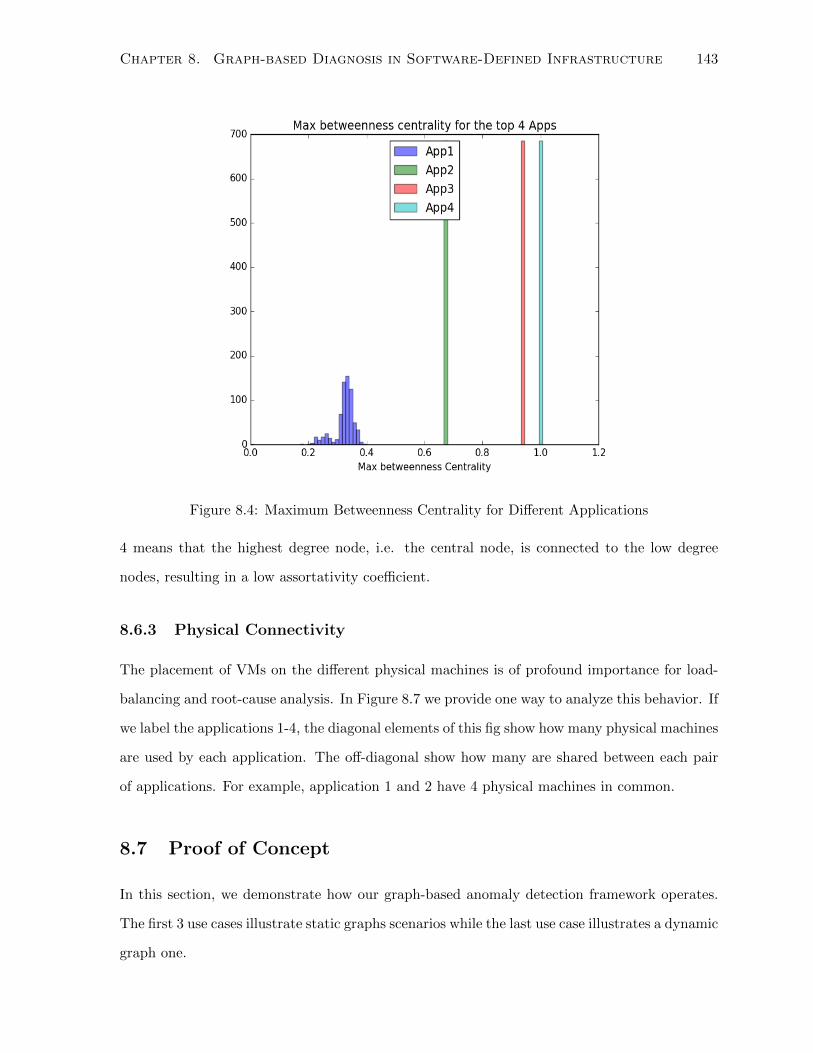
Chapter 8. Graph-based Diagnosis in Software-Defined Infrastructure 143
Figure 8.4: Maximum Betweenness Centrality for Different Applications
4 means that the highest degree node, i.e. the central node, is connected to the low degree
nodes, resulting in a low assortativity coefficient.
8.6.3 Physical Connectivity
The placement of VMs on the different physical machines is of profound importance for load-
balancing and root-cause analysis. In Figure 8.7 we provide one way to analyze this behavior. If
we label the applications 1-4, the diagonal elements of this fig show how many physical machines
are used by each application. The off-diagonal show how many are shared between each pair
of applications. For example, application 1 and 2 have 4 physical machines in common.
8.7 Proof of Concept
In this section, we demonstrate how our graph-based anomaly detection framework operates.
The first 3 use cases illustrate static graphs scenarios while the last use case illustrates a dynamic
graph one.
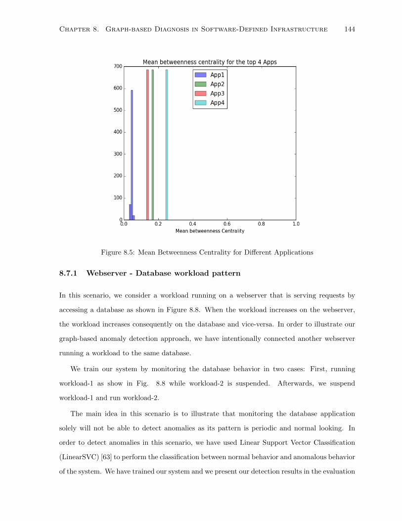
Chapter 8. Graph-based Diagnosis in Software-Defined Infrastructure 144
Figure 8.5: Mean Betweenness Centrality for Different Applications
8.7.1 Webserver - Database workload pattern
In this scenario, we consider a workload running on a webserver that is serving requests by
accessing a database as shown in Figure 8.8. When the workload increases on the webserver,
the workload increases consequently on the database and vice-versa. In order to illustrate our
graph-based anomaly detection approach, we have intentionally connected another webserver
running a workload to the same database.
We train our system by monitoring the database behavior in two cases: First, running
workload-1 as show in Fig. 8.8 while workload-2 is suspended. Afterwards, we suspend
workload-1 and run workload-2.
The main idea in this scenario is to illustrate that monitoring the database application
solely will not be able to detect anomalies as its pattern is periodic and normal looking. In
order to detect anomalies in this scenario, we have used Linear Support Vector Classification
(LinearSVC) [63] to perform the classification between normal behavior and anomalous behavior
of the system. We have trained our system and we present our detection results in the evaluation
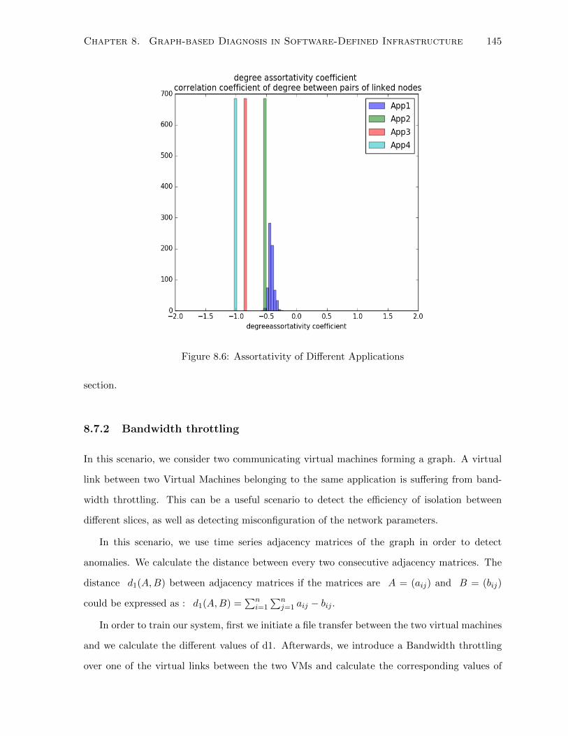
Chapter 8. Graph-based Diagnosis in Software-Defined Infrastructure 145
Figure 8.6: Assortativity of Different Applications
section.
8.7.2 Bandwidth throttling
In this scenario, we consider two communicating virtual machines forming a graph. A virtual
link between two Virtual Machines belonging to the same application is suffering from band-
width throttling. This can be a useful scenario to detect the efficiency of isolation between
different slices, as well as detecting misconfiguration of the network parameters.
In this scenario, we use time series adjacency matrices of the graph in order to detect
anomalies. We calculate the distance between every two consecutive adjacency matrices. The
distance d1(A,B) between adjacency matrices if the matrices are A = (aij) and B = (bij)
could be expressed as : d1(A,B) =∑n
i=1
∑nj=1 aij − bij .
In order to train our system, first we initiate a file transfer between the two virtual machines
and we calculate the different values of d1. Afterwards, we introduce a Bandwidth throttling
over one of the virtual links between the two VMs and calculate the corresponding values of
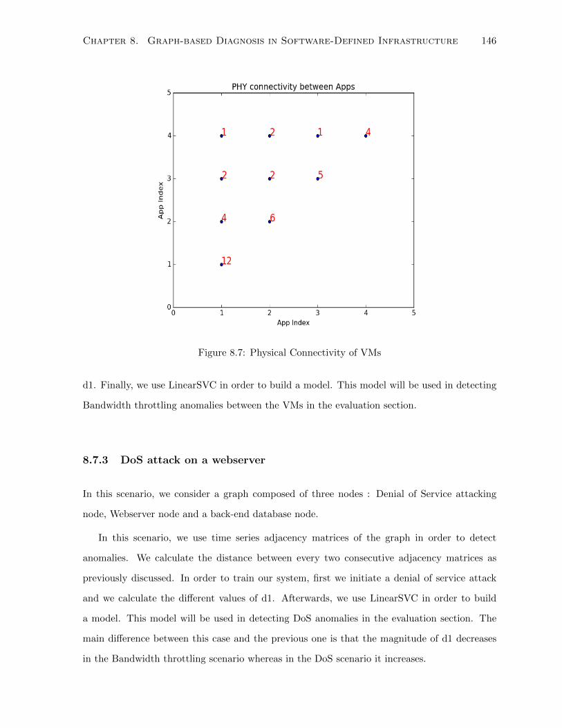
Chapter 8. Graph-based Diagnosis in Software-Defined Infrastructure 146
Figure 8.7: Physical Connectivity of VMs
d1. Finally, we use LinearSVC in order to build a model. This model will be used in detecting
Bandwidth throttling anomalies between the VMs in the evaluation section.
8.7.3 DoS attack on a webserver
In this scenario, we consider a graph composed of three nodes : Denial of Service attacking
node, Webserver node and a back-end database node.
In this scenario, we use time series adjacency matrices of the graph in order to detect
anomalies. We calculate the distance between every two consecutive adjacency matrices as
previously discussed. In order to train our system, first we initiate a denial of service attack
and we calculate the different values of d1. Afterwards, we use LinearSVC in order to build
a model. This model will be used in detecting DoS anomalies in the evaluation section. The
main difference between this case and the previous one is that the magnitude of d1 decreases
in the Bandwidth throttling scenario whereas in the DoS scenario it increases.
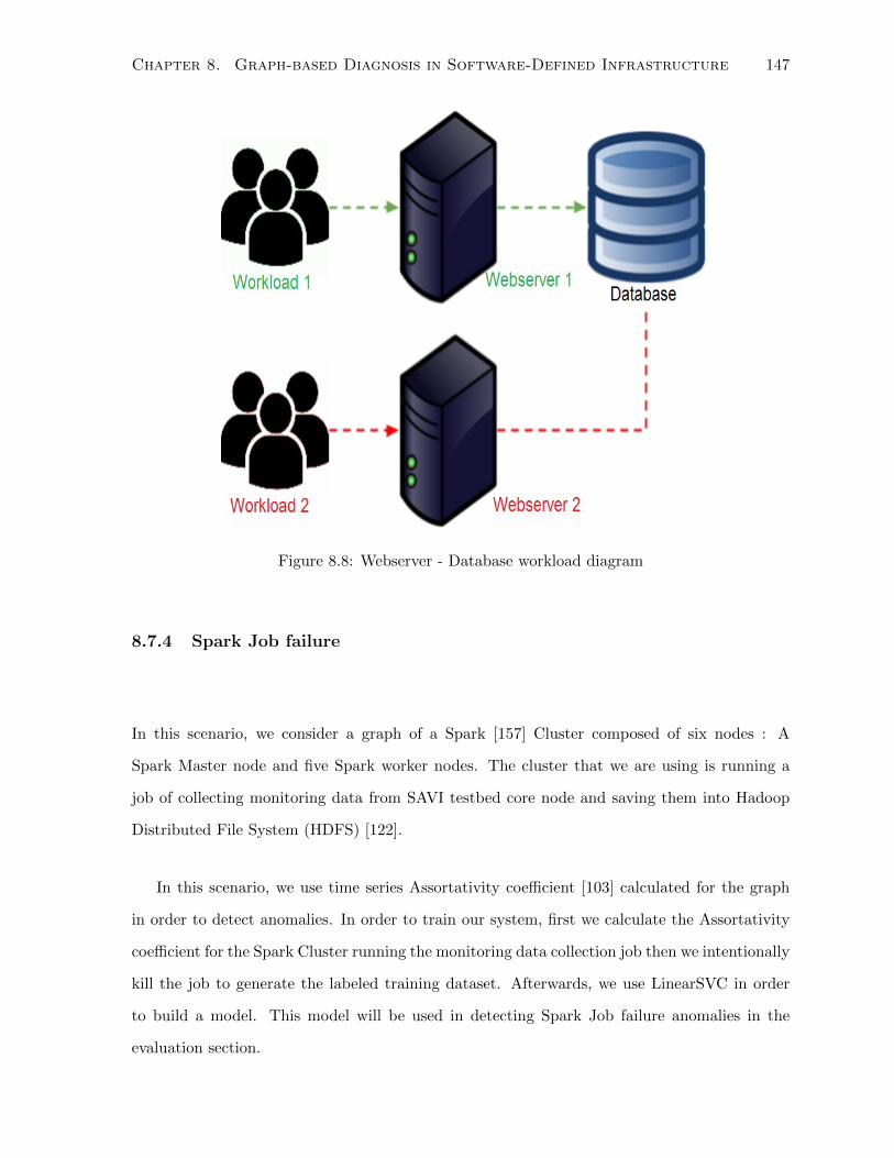
Chapter 8. Graph-based Diagnosis in Software-Defined Infrastructure 147
Figure 8.8: Webserver - Database workload diagram
8.7.4 Spark Job failure
In this scenario, we consider a graph of a Spark [157] Cluster composed of six nodes : A
Spark Master node and five Spark worker nodes. The cluster that we are using is running a
job of collecting monitoring data from SAVI testbed core node and saving them into Hadoop
Distributed File System (HDFS) [122].
In this scenario, we use time series Assortativity coefficient [103] calculated for the graph
in order to detect anomalies. In order to train our system, first we calculate the Assortativity
coefficient for the Spark Cluster running the monitoring data collection job then we intentionally
kill the job to generate the labeled training dataset. Afterwards, we use LinearSVC in order
to build a model. This model will be used in detecting Spark Job failure anomalies in the
evaluation section.
Chapter 8. Graph-based Diagnosis in Software-Defined Infrastructure 148
8.8 Evaluation
In order to evaluate our system, we have conducted several experiments to verify our approach
in detecting anomalies. We performed our experiments in the core node of the SAVI testbed,
composed of over 20 physical servers hosting a few hundred VMs. We use the OpenStack
and OpenFlow to collect data about the various elements in our network. Collected metrics
include: CPU utilization, amount of disk read and write data, amount of memory read and write
data, and network bandwidth between each pair of VMs. Our experiments are reproducible
by requesting access to SAVI testbed from [2]. The details about the metrics available from
Openstack can be found in [37]. We use Hadoop as our distributed file-system for data storage
and Spark as our analytics framework. In the following subsections, we present the verification
for each use case described in the Proof of Concept section.
Webserver - Database workload pattern
We have trained our system using 5 hours of data. Afterwards, we tested our system using
1.5 hours of data. We used the CPU Utilization metrics collected from the Webserver and
Database. Figure 8.9 shows the testing phase of our system. The dash-doted curve represents
the CPU Utilization of the Webserver, the dashed curve represents the CPU utilization of the
Database. The solid curve represents the labels of the test data that we know beforehand ;
high means anomaly, low means normal behavior. The dots represent the predicted labels of
the data using LinearSVC. Our system was able to detect the 11 anomalies accurately as shown
in Figure 8.9.
Bandwidth throttling
We have setup two Virtual Machines with xlarge flavor that has 160GB of disk. We have
initiated a file transfer operation between the two VMs. The file size was 100GB with a transfer
rate 10 Mbps between the two VMs.The throttling value in the training phase was fixed at 512
kbps. The training set for LinearSVC was 134 data points. Afterwards, we tested our system
by repeating the same experiment but while having random varying throttling value between
1 Mbps and 5 Mbps as shown in Figure 8.10. The dotted curve represents the time varying
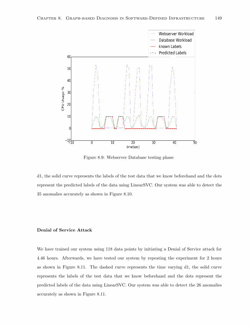
Chapter 8. Graph-based Diagnosis in Software-Defined Infrastructure 149
Figure 8.9: Webserver Database testing phase
d1, the solid curve represents the labels of the test data that we know beforehand and the dots
represent the predicted labels of the data using LinearSVC. Our system was able to detect the
35 anomalies accurately as shown in Figure 8.10.
Denial of Service Attack
We have trained our system using 118 data points by initiating a Denial of Service attack for
4.46 hours. Afterwards, we have tested our system by repeating the experiment for 2 hours
as shown in Figure 8.11. The dashed curve represents the time varying d1, the solid curve
represents the labels of the test data that we know beforehand and the dots represent the
predicted labels of the data using LinearSVC. Our system was able to detect the 26 anomalies
accurately as shown in Figure 8.11.
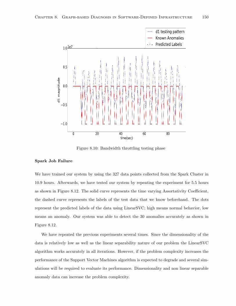
Chapter 8. Graph-based Diagnosis in Software-Defined Infrastructure 150
Figure 8.10: Bandwidth throttling testing phase
Spark Job Failure
We have trained our system by using the 327 data points collected from the Spark Cluster in
10.9 hours. Afterwards, we have tested our system by repeating the experiment for 5.5 hours
as shown in Figure 8.12. The solid curve represents the time varying Assortativity Coefficient,
the dashed curve represents the labels of the test data that we know beforehand. The dots
represent the predicted labels of the data using LinearSVC; high means normal behavior, low
means an anomaly. Our system was able to detect the 30 anomalies accurately as shown in
Figure 8.12.
We have repeated the previous experiments several times. Since the dimensionality of the
data is relatively low as well as the linear separability nature of our problem the LinearSVC
algorithm works accurately in all iterations. However, if the problem complexity increases the
performance of the Support Vector Machines algorithm is expected to degrade and several sim-
ulations will be required to evaluate its performance. Dimensionality and non linear separable
anomaly data can increase the problem complexity.
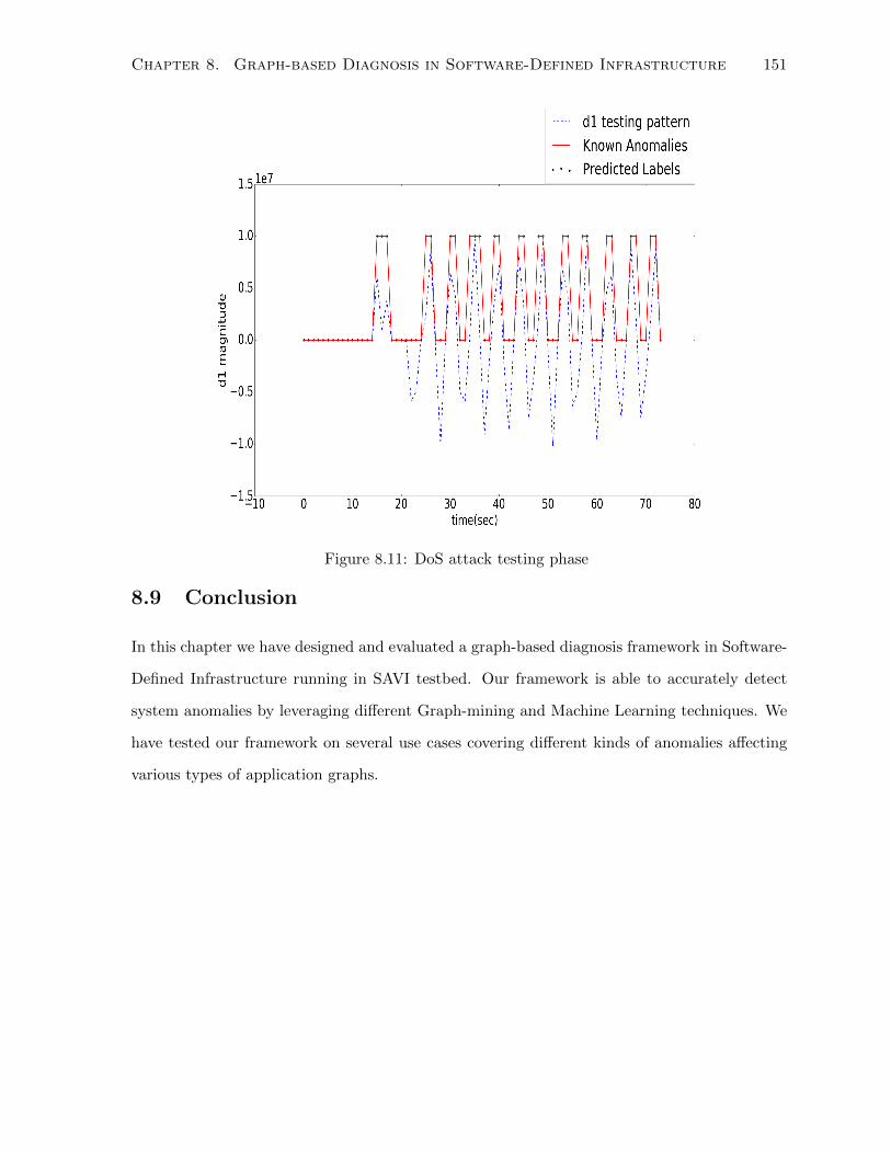
Chapter 8. Graph-based Diagnosis in Software-Defined Infrastructure 151
Figure 8.11: DoS attack testing phase
8.9 Conclusion
In this chapter we have designed and evaluated a graph-based diagnosis framework in Software-
Defined Infrastructure running in SAVI testbed. Our framework is able to accurately detect
system anomalies by leveraging different Graph-mining and Machine Learning techniques. We
have tested our framework on several use cases covering different kinds of anomalies affecting
various types of application graphs.
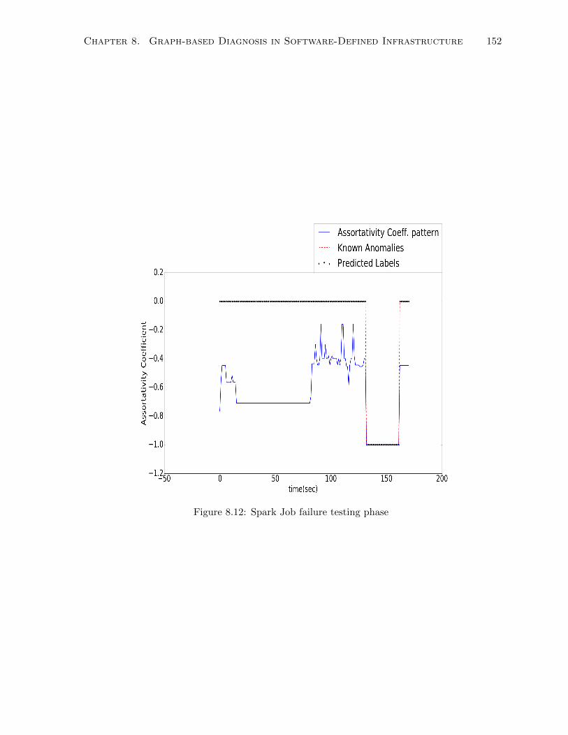
Chapter 8. Graph-based Diagnosis in Software-Defined Infrastructure 152
Figure 8.12: Spark Job failure testing phase
Chapter 9
Auto-Scaling and Anomaly
Detection in Software-Defined
Infrastructure
9.1 Context
In continuation of Chapter 8, we resume our study of how the infrastructure controller can
accurately and securely manage the cloud computing resources. The software-defined nature
of next-generation cloud environments are a great enabler for building efficient resource man-
agement frameworks. The elasticity of the cloud environment enables scaling up resources
according to the customer’s demand, offering a significant advantage over dedicated private
infrastructure systems. For example, in cloud-RAN the system load is directly dependent on
the number of active user which exhibits strong cyclo-stationary behavior. However, the effi-
ciency of such auto-scaling systems are limited by their ability to identify anomalous patterns
in the customer’s behavior in order to avoid unnecessary scaling when the system is breached.
Motivated by these two lines of reasoning, we propose a framework for an anomaly-aware auto-
scaling system. We employ a stochastic control framework that is able to predict the future
states of the system and identify the need to pro-actively scale the resources, as well as to
detect anomalies if the observed state is significantly different from the predicted one. We have
153
Chapter 9. Auto-Scaling and Anomaly Detection in Software-Defined Infrastructure154
implemented our framework as part of the SAVI testbed. We have leveraged the Spark Big-
Data platform to make our framework scalable with the large number of resources present in
the cloud. We present experimental results where we have observed an efficient 95% prediction
accuracy as well as over 90% anomaly detection accuracy.
9.2 Introduction
A significant challenge in cloud systems is to automatically scale the resources according to
the customer’s needs [85]. The infrastructure provider should be able to observe the the usage
pattern, and release any idle resources to avoid overcharging the customers. More important, is
the ability to upgrade the assigned resources to prevent the possibility of performance bottle-
necks. However, in the current networked world, the ability to estimate a customer’s behavior
is hindered by the various security attacks that might breach its system [145]. For this reason,
we provide the first, to our knowledge, study for joint anomaly-detection and auto-scaling for
software-defined infrastructure. The key concept in our solution is to employ a non-parametric
prediction scheme. Such a scheme should be able to not only predict the future state of the
system, but also provide the confidence level of its prediction. Using the predicted state and
its confidence level, an automated management system will then decide if the resource is to
be scaled up or down, and when the actual state is observed, decide whether it is normal or
anomalous.
In this chapter, we continue the theme we started in Chapter 8 about the auto-scaling and
anomaly detection in cloud computing systems. In particular, we study how auto-scaling can
be combined with anomaly detection to provide a general resource management framework for
cloud resources. The system architecture under study is shown in Fig. 9.1. This is the same
architecture used in the previous chapter where the infrastructure controller reads the state of
the user processes and the computing resources in order to come up with the necessary scaling
and migration decisions. In this chapter we focus on how auto-scaling can be designed jointly
with anomaly detection, unlike the previous chapter where we focused solely on the anomaly
detection part. We propose a pro-active auto-scaling policy where the infrastructure controller
predicts the future state of the system, e.g. the computing needs of the user process. In wire-
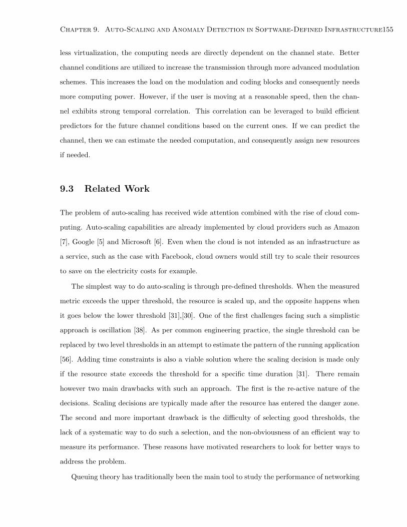
Chapter 9. Auto-Scaling and Anomaly Detection in Software-Defined Infrastructure155
less virtualization, the computing needs are directly dependent on the channel state. Better
channel conditions are utilized to increase the transmission through more advanced modulation
schemes. This increases the load on the modulation and coding blocks and consequently needs
more computing power. However, if the user is moving at a reasonable speed, then the chan-
nel exhibits strong temporal correlation. This correlation can be leveraged to build efficient
predictors for the future channel conditions based on the current ones. If we can predict the
channel, then we can estimate the needed computation, and consequently assign new resources
if needed.
9.3 Related Work
The problem of auto-scaling has received wide attention combined with the rise of cloud com-
puting. Auto-scaling capabilities are already implemented by cloud providers such as Amazon
[7], Google [5] and Microsoft [6]. Even when the cloud is not intended as an infrastructure as
a service, such as the case with Facebook, cloud owners would still try to scale their resources
to save on the electricity costs for example.
The simplest way to do auto-scaling is through pre-defined thresholds. When the measured
metric exceeds the upper threshold, the resource is scaled up, and the opposite happens when
it goes below the lower threshold [31],[30]. One of the first challenges facing such a simplistic
approach is oscillation [38]. As per common engineering practice, the single threshold can be
replaced by two level thresholds in an attempt to estimate the pattern of the running application
[56]. Adding time constraints is also a viable solution where the scaling decision is made only
if the resource state exceeds the threshold for a specific time duration [31]. There remain
however two main drawbacks with such an approach. The first is the re-active nature of the
decisions. Scaling decisions are typically made after the resource has entered the danger zone.
The second and more important drawback is the difficulty of selecting good thresholds, the
lack of a systematic way to do such a selection, and the non-obviousness of an efficient way to
measure its performance. These reasons have motivated researchers to look for better ways to
address the problem.
Queuing theory has traditionally been the main tool to study the performance of networking
Chapter 9. Auto-Scaling and Anomaly Detection in Software-Defined Infrastructure156
Baseband Processing, Lookup tables for faster
processing and switch abstraction
Baseband Processing, Lookup tables for faster
processing and switch abstraction
FrontHaul Network
coding scrambling modulation
Bin
ary
inp
ut
bit
s
I/Q
Sign
als
Cloud
computing
resources
Remote Radio
heads
User Process
Infrastructure Controller
Computing
resources scaling
and migration
Clo
ud
Net
wo
rk F
abri
c
VM utilization
Scaling decisions
End-users
Figure 9.1: Cloud-RAN Architecture - Auto-scaling and anomaly detection
Chapter 9. Auto-Scaling and Anomaly Detection in Software-Defined Infrastructure157
Figure 9.2: SAVI testbed Architecture
and servers applications [92]. The theory has been used to model cloud environments, mainly
through G/G/1 or G/G/n models [13], [142]. The main goal of this analysis is to find the
expected peak load, the necessary resources needed to serve a certain workload, or the mean
response time for requests. As such, queuing theory is more appropriate for planning purposes
rather on-line decision making. Queuing theory suffers, to some extent, from the rigidity of
its models. Additionally, it is typically hard to extend the traditional models to new scenarios
such as MapReduce applications with master and slave nodes. Moreover, the queue control
problems, when they are studied, typically end up with threshold-based decisions anyways [15].
The controller design aspect of the auto-scaling problem has naturally led to the adop-
tion of techniques from the field of control theory [105]. The main goal here is the controller
design. Controller classes such as proportionalintegral (PI), proportionalderivative (PD) and
proportionalintegralderivative (PID) have been proposed [81],[164]. The main challenge in the
controller design process is choosing the transfer function, state-space function or the perfor-
mance model [85]. This difficulty can be partially overcome by adopting adaptive controllers,
Chapter 9. Auto-Scaling and Anomaly Detection in Software-Defined Infrastructure158
which can be considered as special cases of the more general reinforcement learning problem
[135].
The ability to make the scaling decision pro-actively involves predicting the future state of
the resource [137]. Predictive analysis combined with re-enforcement learning are considered in
the literature to be the most promising solutions [85]. These techniques have been studied in
the literature in [137],[39],[112],[150] . However, a major challenge that has not been addressed
before is the ability to correctly distinguish the true system resource states from the anomalous
and to consider such distinction when making the scaling decisions.
Our main contributions are : we provide a general formulation for the stochastic control
problem of joint anomaly detection and auto-scaling in cloud computing systems. We also
provide the practical aspects of the problem from our interaction with the implementation in
OpenStack. Based on these two points, we propose a solution policy that can pro-actively
decide about the scaling and re-actively detect the anomalies. We discuss our implementation
of the framework within the SAVI testbed. We provide experimental results for the framework
including prediction accuracy, anomaly-detection accuracy, as well as other aspects of how the
involved components work within OpenStack.
9.4 System Model
Consider a cloud computing system where a cloud customer, or equivalently an application,
needs a set of resources V. Due to anomalous behaviors or security attacks, the customer is
actually provided with the resource set V, where typically V ⊂ V. Let f : V → R be the cost
function mapping the given set of resources to the actual cost. Our optimization problem is
then as follows:
Problem 9.1:
minV
E{f(V) + ν |M|
}s.t. g(V) ≤ δ
M = V − V
(9.1)
Chapter 9. Auto-Scaling and Anomaly Detection in Software-Defined Infrastructure159
where g(.) is a quality of service measure function, andM is the mismatch, possibly due to
anomalies, between the needed and assigned resources and |M| is its cardinality, ν is a weight
parameter that determines the trade-off between the two terms of the objective function, and
δ is the QoS parameter. The goal of the optimization problem is to minimize the expected cost
incurred and avoid assigning any unneeded resources.
Problem (9.1) belongs to a class of problems known as stochastic optimization problems
[109]. Outside of using Bellman’s equation [22], which suffers from the curse of dimensionality,
this class of problems has no systematic way for finding its solutions [109]. The general approach
to solve these problems is as follows:
1. Define the set of observable states of the system S.
2. Define the action set A.
3. Define the policy pθ : S → A as the state-action mapping parametrized by θ.
4. Optimize the policy as a function of its parameters p = arg maxθ pθ
In order to define our policy, we have to specify more details about problem (1).
9.4.1 Cost Measure and Quality of Service
In this chapter, we adopt the following notations:
• V = {vhi : i ∈ {1, 2, ..., Nv}, h ∈ H}
• f(V) =∑h∈H
ch
∣∣∣Vh∣∣∣• g(V) = P(u(vhi ) ≥ γ) ∀ vhi ∈ V
where h denotes the flavor of the VM vhi , Nv is the number of VMs in the set V, and H is
the set of available flavors, typically small, medium and large, ch is the cost associated with a
specific flavor.
The first condition states that the set of resources we consider is the set of virtual machines
(VMs). Each virtual machine has an index, and a flavor. The flavor of the VM determines
its computing power in terms of CPU, memory and so on. The second condition states that
Chapter 9. Auto-Scaling and Anomaly Detection in Software-Defined Infrastructure160
the cost incurred is proportional to the number of assigned VMs, and the cost of each VM
is dependent upon its flavor. The third condition is our QoS metric, which states that the
probability that the utilization of the VM exceeds a specific threshold γ should be below a
certain value δ, as in 9.1.
In such a case, the state and action are specifically defined as follows:
• s(t) = u(vhi , t) ∀ vhi ∈ V
• a(vhi ) = vh+1i , a(vhi ) = vh−1i
The state at time t is defined as the utilization levels of all assigned VMs. The action applied
on a VM vhi can either upgrade its flavor to the next level vh+1i , or downgrade it to the previous
one vh−1i . Note that in general we could transition between any two flavors, not necessarily
consecutive. These definitions of actions and states are compatible with the enabling technolo-
gies in the cloud systems, as will be explained in the next section.
Before we discuss the policy, we have to consider some additional aspects of the problem:
Re-Active versus Pro-Active
Auto-scaling decisions can be made either reactively or pro-actively [85]. Reactively means
that we observe the state first, and then decide the action. On the other hand, a pro-active
decision first involves some form of prediction, then we base our action upon the predicted state.
Intuitively, re-active techniques are less computationally demanding than pro-active ones, while
the latter are expected to outperform the former due to their anticipative nature. The decision
to choose which technique to go with depends on the frequency of the state observations and
the time needed to execute the action. In our case, when OpenStack receives a re-size request,
it can either re-scale the VM on the same physical machine, or migrate it to another one. The
migration process takes on average 10 times the time of the same-machine scaling (around
20 minutes for migration from our experiments). Note that depending on the application
requirements, even the no-migration re-size time might be too long. For such reasons, we have
decided to proceed with a pro-active policy.
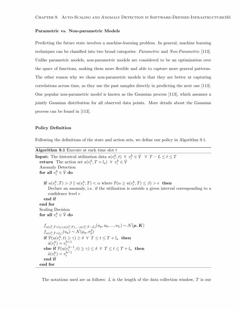
Chapter 9. Auto-Scaling and Anomaly Detection in Software-Defined Infrastructure161
Parametric vs. Non-parametric Models
Predicting the future state involves a machine-learning problem. In general, machine learning
techniques can be classified into two broad categories: Parametric and Non-Parametric [113].
Unlike parametric models, non-parametric models are considered to be an optimization over
the space of functions, making them more flexible and able to capture more general patterns.
The other reason why we chose non-parametric models is that they are better at capturing
correlations across time, as they use the past samples directly in predicting the next one [113].
One popular non-parametric model is known as the Gaussian process [113], which assumes a
jointly Gaussian distribution for all observed data points. More details about the Gaussian
process can be found in [113].
Policy Definition
Following the definitions of the state and action sets, we define our policy in Algorithm 9.1.
Algorithm 9.1 Execute at each time slot t
Input: The historical utilization data u(vhi , t) ∀ vhi ∈ V ∀ T − L ≤ t ≤ Treturn The action set a(vhi , T + la) ∀ vhi ∈ VAnomaly Detectionfor all vhi ∈ V do
if u(vhi , T ) > β || u(vhi , T ) < α where P(α ≥ u(vhi , T ) ≤ β) > e thenDeclare an anomaly, i.e. if the utilization is outside a given interval corresponding to aconfidence level e
end ifend forScaling Decisionfor all vhi ∈ V do
fu(vhi ,T+la),u(vhi ,T ),...,u(vhi ,T−L)(up, u0, ..., uL) ∼ N (µ,K)
fu(vhi ,T+la)(up) ∼ N (µp, σ
2p)
if P(u(vhi , t) ≥ γ) ≥ δ ∀ T ≤ t ≤ T + la thena(vhi ) = vh+1
i
else if P(u(vh−1i , t) ≥ γ) ≤ δ ∀ T ≤ t ≤ T + la thena(vhi ) = vh−1i
end ifend for
The notations used are as follows: L is the length of the data collection window, T is our
Chapter 9. Auto-Scaling and Anomaly Detection in Software-Defined Infrastructure162
operation interval, la is the look ahead interval, e is the confidence level and β−α is the length of
the confidence interval, and N (µ,K),N (µp, σ2p) are the Gaussian distributions resulting from
fitting the Gaussian process.
The process we follow in Algorithm 9.1 is as follows: the Gaussian process model is trained
for each VM. The main feature used in the training is the CPU utilization. We have used
both the CPU utilization of that VM as well as that of its connected VMs. The networking
information is available from OpenFlow.
Once the training phase is done, two decisions have to made by the algorithm. The first
decision is whether the observed state is anomalous. From the the Gaussian process model, we
predict the expected value as well as the confidence interval for the next time slot. When the
next measurement comes in, an anomaly is declared if the observed data point is outside the
specified confidence interval, for example a 95% confidence interval can be used in such a case.
If the observation is declared to be safe, then use the Gaussian process to predict the next state.
The second decision is the scaling decision. Using the Gaussian distribution assumption, we
can estimate the probability that the QoS constraint is violated. If such probability exceeds a
certain limit, then an up-scaling decision is made. On the other hand, in order for the policy
to minimize the objective function, we consider the case for a down-scaling. If a down-scaling
can be made while keeping the QoS constraint intact, then we proceed with the down-scaling.
Note that depending on the rate of change of the resource utilization, we might need to do a
multi-level up-scale or down-scale.
Note that the proposed algorithm does not solve problem (9.1) in its original form, as this is
typically infeasible for the stochastic optimization problems. Instead, the proposed policy tries
to achieve the same goals, i.e. resource scaling and anomaly detection, based on the capabilities
of our practical system.
The following parameters control the performance of the algorithm. For the anomaly de-
tection part, e is the level of confidence and [α, β] is the corresponding interval. If e is chosen
to be 95%, then α = µp − 3σp and β = µp + 3σp. L is the window of past measurements that
are used in predicting the next state. Larger window sizes typically result in better predictions,
but at the expense of increased complexity. The other parameter is la which is the look ahead
time. Typically for a Gaussian process, the further ahead we are trying to predict, the less
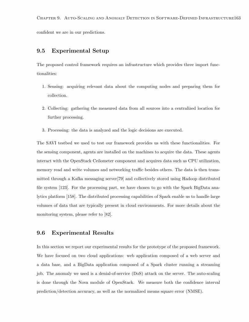
Chapter 9. Auto-Scaling and Anomaly Detection in Software-Defined Infrastructure163
confident we are in our predictions.
9.5 Experimental Setup
The proposed control framework requires an infrastructure which provides three import func-
tionalities:
1. Sensing: acquiring relevant data about the computing nodes and preparing them for
collection.
2. Collecting: gathering the measured data from all sources into a centralized location for
further processing.
3. Processing: the data is analyzed and the logic decisions are executed.
The SAVI testbed we used to test our framework provides us with these functionalities. For
the sensing component, agents are installed on the machines to acquire the data. These agents
interact with the OpenStack Ceilometer component and acquires data such as CPU utilization,
memory read and write volumes and networking traffic besides others. The data is then trans-
mitted through a Kafka messaging server[79] and collectively stored using Hadoop distributed
file system [123]. For the processing part, we have chosen to go with the Spark BigData ana-
lytics platform [158]. The distributed processing capabilities of Spark enable us to handle large
volumes of data that are typically present in cloud environments. For more details about the
monitoring system, please refer to [82].
9.6 Experimental Results
In this section we report our experimental results for the prototype of the proposed framework.
We have focused on two cloud applications: web application composed of a web server and
a data base, and a BigData application composed of a Spark cluster running a streaming
job. The anomaly we used is a denial-of-service (DoS) attack on the server. The auto-scaling
is done through the Nova module of OpenStack. We measure both the confidence interval
prediction/detection accuracy, as well as the normalized means square error (NMSE).
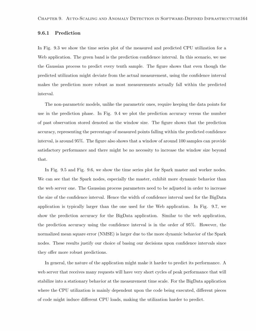
Chapter 9. Auto-Scaling and Anomaly Detection in Software-Defined Infrastructure164
9.6.1 Prediction
In Fig. 9.3 we show the time series plot of the measured and predicted CPU utilization for a
Web application. The green band is the prediction confidence interval. In this scenario, we use
the Gaussian process to predict every tenth sample. The figure shows that even though the
predicted utilization might deviate from the actual measurement, using the confidence interval
makes the prediction more robust as most measurements actually fall within the predicted
interval.
The non-parametric models, unlike the parametric ones, require keeping the data points for
use in the prediction phase. In Fig. 9.4 we plot the prediction accuracy versus the number
of past observation stored denoted as the window size. The figure shows that the prediction
accuracy, representing the percentage of measured points falling within the predicted confidence
interval, is around 95%. The figure also shows that a window of around 100 samples can provide
satisfactory performance and there might be no necessity to increase the window size beyond
that.
In Fig. 9.5 and Fig. 9.6, we show the time series plot for Spark master and worker nodes.
We can see that the Spark nodes, especially the master, exhibit more dynamic behavior than
the web server one. The Gaussian process parameters need to be adjusted in order to increase
the size of the confidence interval. Hence the width of confidence interval used for the BigData
application is typically larger than the one used for the Web application. In Fig. 9.7, we
show the prediction accuracy for the BigData application. Similar to the web application,
the prediction accuracy using the confidence interval is in the order of 95%. However, the
normalized mean square error (NMSE) is larger due to the more dynamic behavior of the Spark
nodes. These results justify our choice of basing our decisions upon confidence intervals since
they offer more robust predictions.
In general, the nature of the application might make it harder to predict its performance. A
web server that receives many requests will have very short cycles of peak performance that will
stabilize into a stationary behavior at the measurement time scale. For the BigData application
where the CPU utilization is mainly dependent upon the code being executed, different pieces
of code might induce different CPU loads, making the utilization harder to predict.
Chapter 9. Auto-Scaling and Anomaly Detection in Software-Defined Infrastructure165
9.6.2 Anomaly Detection
In Fig. 9.8 we have a time series plot of the server CPU utilization in the presence of DoS
attacks. The server runs for around half an hour and then gets a DoS attack for a period of
five minutes, visible as the spikes in the CPU utilization. We use the data gathered during
the normal 30 minutes to predict the states during the anomalous 5 minute duration. Note
that we receive 2 measurements during the 5 minutes interval. We declare an anomaly if the
measurement lies outside the predicted confidence interval. Since we always have two anomalous
points at a time, our anomaly detection accuracy for each single DoS attack is either 0%, 50%
or 100%. . We also steadily increase the normal load with time. The detection accuracies, i.e.
the percentage of points declared as anomalies, are shown in Fig. 9.9, where they are plotted
versus the mean load of the server during the normal operation state.
Our main observation from this experiment is that there is a trade-off between the ability
to detect anomalies and the utilization level of the VM. As the mean utilization level goes
up, the anomaly detection accuracy goes down. The explanation for this phenomena is as
follows: when the VM is operating at 20% utilization for example, then it is easy to declare
the 90% as an anomaly. Compare this with the case when the normal state is around 80%
utilization, which makes a change to 90% utilization very probable. Going back to our objective
function defined in problem 1, we see that there is a trade-off between the two components of
the objective function, namely minimizing the used resources and maximizing the anomaly
detection accuracy. Minimizing the used resources means that the assigned VMs have to be
operating near their maximum utilization, which makes the anomalies harder to detect.
One point that has not been studied in this chapter is closing the control loop when the
anomaly has been detected. This involves the action needed to be taken to counter the anomaly,
as well as an efficient state update mechanism that takes into account our confidence of the
measurements.
9.7 Conclusion
In this chapter we have proposed a control framework for joint anomaly detection and auto-
scaling in software-defined infrastructures. We have proposed policy based on the Gaussian
Chapter 9. Auto-Scaling and Anomaly Detection in Software-Defined Infrastructure166
200 400 600 800 1000 1200 1400 1600 1800Time +1.2303e7
18
20
22
24
26
28
30
Utilization
UtilizationPrediction
Figure 9.3: Example of CPU utilization Prediction for a Web application
0 50 100 150 200 250 300Window Size
0.04
0.06
0.08
0.10
0.12
0.14
0.16
Error
NMSEConfidence Error
Figure 9.4: Prediction Accuracy for a Web application
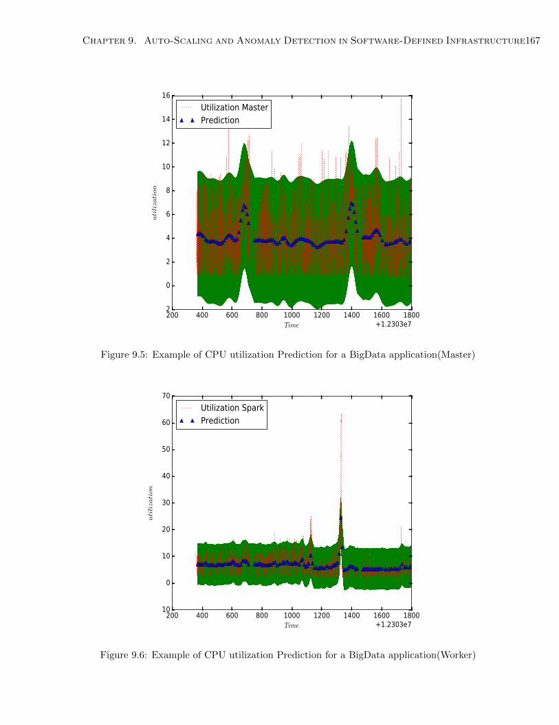
Chapter 9. Auto-Scaling and Anomaly Detection in Software-Defined Infrastructure167
200 400 600 800 1000 1200 1400 1600 1800Time +1.2303e7
−2
0
2
4
6
8
10
12
14
16
utilization
Utilization MasterPrediction
Figure 9.5: Example of CPU utilization Prediction for a BigData application(Master)
200 400 600 800 1000 1200 1400 1600 1800Time +1.2303e7
−10
0
10
20
30
40
50
60
70
utilization
Utilization SparkPrediction
Figure 9.6: Example of CPU utilization Prediction for a BigData application(Worker)
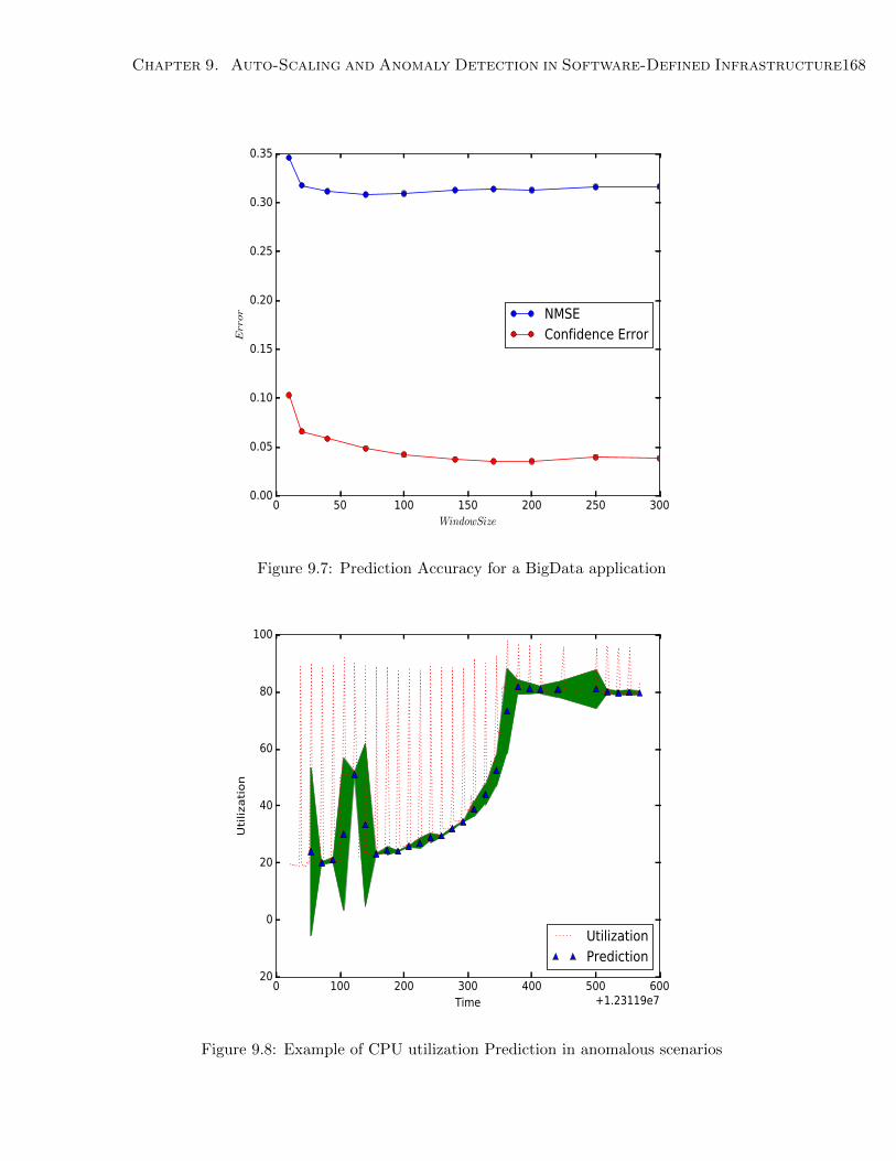
Chapter 9. Auto-Scaling and Anomaly Detection in Software-Defined Infrastructure168
0 50 100 150 200 250 300WindowSize
0.00
0.05
0.10
0.15
0.20
0.25
0.30
0.35
Error NMSE
Confidence Error
Figure 9.7: Prediction Accuracy for a BigData application
0 100 200 300 400 500 600Time +1.23119e7
−20
0
20
40
60
80
100
Utilization
UtilizationPrediction
Figure 9.8: Example of CPU utilization Prediction in anomalous scenarios
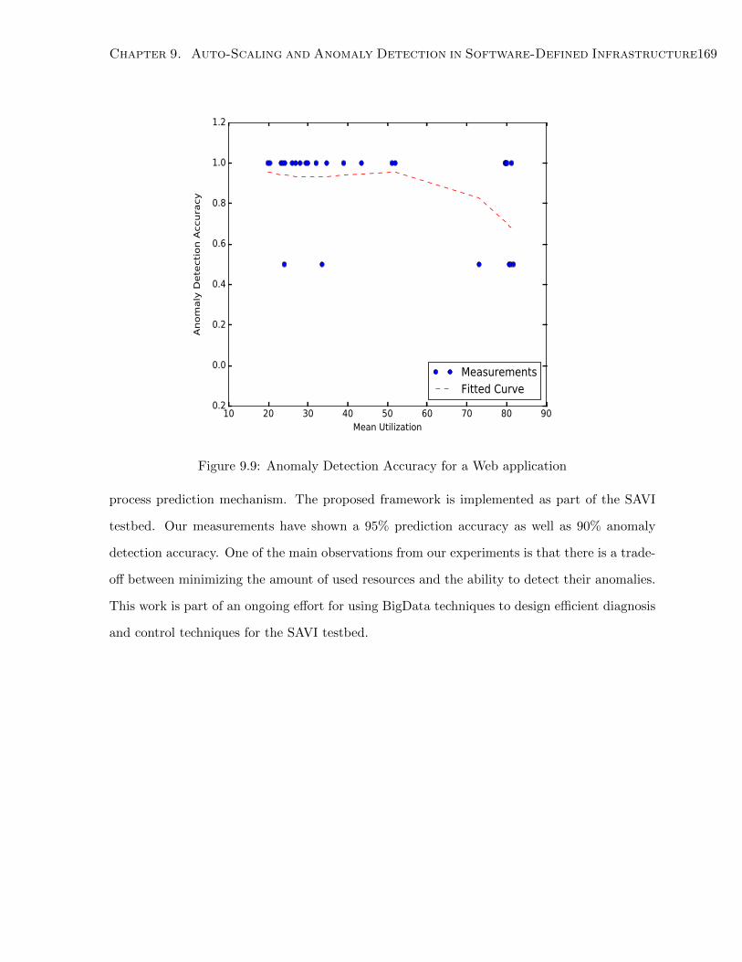
Chapter 9. Auto-Scaling and Anomaly Detection in Software-Defined Infrastructure169
10 20 30 40 50 60 70 80 90Mean Utilization
−0.2
0.0
0.2
0.4
0.6
0.8
1.0
1.2
Anomal Detection Accurac
MeasurementsFitted Curve
Figure 9.9: Anomaly Detection Accuracy for a Web application
process prediction mechanism. The proposed framework is implemented as part of the SAVI
testbed. Our measurements have shown a 95% prediction accuracy as well as 90% anomaly
detection accuracy. One of the main observations from our experiments is that there is a trade-
off between minimizing the amount of used resources and the ability to detect their anomalies.
This work is part of an ongoing effort for using BigData techniques to design efficient diagnosis
and control techniques for the SAVI testbed.

Part IV
Conclusion
170
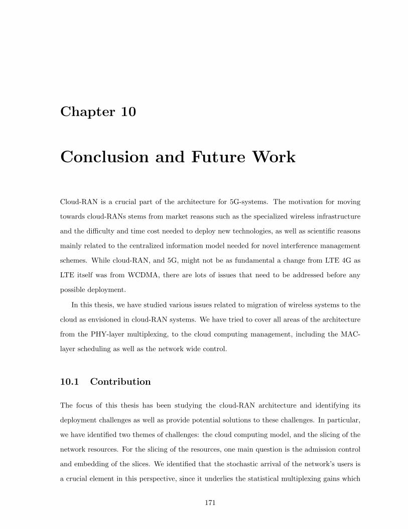
Chapter 10
Conclusion and Future Work
Cloud-RAN is a crucial part of the architecture for 5G-systems. The motivation for moving
towards cloud-RANs stems from market reasons such as the specialized wireless infrastructure
and the difficulty and time cost needed to deploy new technologies, as well as scientific reasons
mainly related to the centralized information model needed for novel interference management
schemes. While cloud-RAN, and 5G, might not be as fundamental a change from LTE 4G as
LTE itself was from WCDMA, there are lots of issues that need to be addressed before any
possible deployment.
In this thesis, we have studied various issues related to migration of wireless systems to the
cloud as envisioned in cloud-RAN systems. We have tried to cover all areas of the architecture
from the PHY-layer multiplexing, to the cloud computing management, including the MAC-
layer scheduling as well as the network wide control.
10.1 Contribution
The focus of this thesis has been studying the cloud-RAN architecture and identifying its
deployment challenges as well as provide potential solutions to these challenges. In particular,
we have identified two themes of challenges: the cloud computing model, and the slicing of the
network resources. For the slicing of the resources, one main question is the admission control
and embedding of the slices. We identified that the stochastic arrival of the network’s users is
a crucial element in this perspective, since it underlies the statistical multiplexing gains which
171
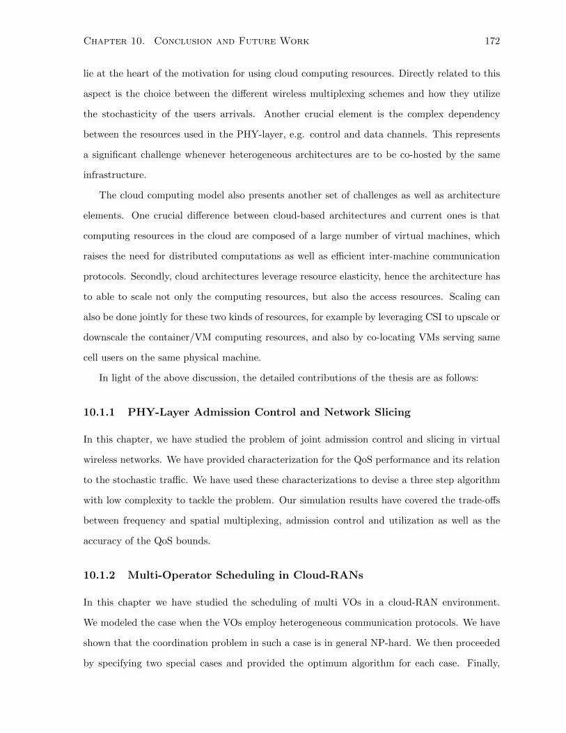
Chapter 10. Conclusion and Future Work 172
lie at the heart of the motivation for using cloud computing resources. Directly related to this
aspect is the choice between the different wireless multiplexing schemes and how they utilize
the stochasticity of the users arrivals. Another crucial element is the complex dependency
between the resources used in the PHY-layer, e.g. control and data channels. This represents
a significant challenge whenever heterogeneous architectures are to be co-hosted by the same
infrastructure.
The cloud computing model also presents another set of challenges as well as architecture
elements. One crucial difference between cloud-based architectures and current ones is that
computing resources in the cloud are composed of a large number of virtual machines, which
raises the need for distributed computations as well as efficient inter-machine communication
protocols. Secondly, cloud architectures leverage resource elasticity, hence the architecture has
to able to scale not only the computing resources, but also the access resources. Scaling can
also be done jointly for these two kinds of resources, for example by leveraging CSI to upscale or
downscale the container/VM computing resources, and also by co-locating VMs serving same
cell users on the same physical machine.
In light of the above discussion, the detailed contributions of the thesis are as follows:
10.1.1 PHY-Layer Admission Control and Network Slicing
In this chapter, we have studied the problem of joint admission control and slicing in virtual
wireless networks. We have provided characterization for the QoS performance and its relation
to the stochastic traffic. We have used these characterizations to devise a three step algorithm
with low complexity to tackle the problem. Our simulation results have covered the trade-offs
between frequency and spatial multiplexing, admission control and utilization as well as the
accuracy of the QoS bounds.
10.1.2 Multi-Operator Scheduling in Cloud-RANs
In this chapter we have studied the scheduling of multi VOs in a cloud-RAN environment.
We modeled the case when the VOs employ heterogeneous communication protocols. We have
shown that the coordination problem in such a case is in general NP-hard. We then proceeded
by specifying two special cases and provided the optimum algorithm for each case. Finally,
Chapter 10. Conclusion and Future Work 173
we proposed a novel neuro-computation heuristic, which is able to handle the general problem
but still provide close-to-optimum results for the special cases studied. The simulation results
confirm the effectiveness of the proposed heuristic and help learn more about the operation of
scheduling in cloud-RAN networks.
10.1.3 Fully Distributed Scheduling in Cloud-RAN Systems
In this chapter we have studied the distributed scheduling problem in Cloud-RAN systems.
Analytical analysis for the Rayleigh channels and maximum throughput scheduler was provided.
We found that distributed scheduling in this case is able to provide around 92% of the centralized
performance. We then extended the scheme to general channels and schedulers by adopting
the classification techniques from machine learning. We discovered two conflicting effects that
depend upon the fairness of the scheduler. In particular, less fair schedulers are easier to
predict, but the penalty for wrong decisions is more severe. With enough training and efficient
parameter selection, the distributed schedulers are able to provide up to 89% of the centralized
performance.
10.1.4 Joint RRH Activation and Clustering in Cloud-RANs
In this chapter we have studied the problem of joint clustering and RRH activation in Cloud-
RAN networks. We have provided a two-step approach to overcome the combinatorial nature of
the problem. The first step involves a linear program approximation to give a feasible solution
using an interference graph. The second step is greedily improving the solution, searching
over both activation and clustering decisions. Our simulation results have shown around 25%
improvement in terms of QoS and energy savings of the joint clustering and activation over the
legacy activation only approach.
10.1.5 Long-term Activation, Clustering and Association in Cloud-RANs
In this chapter we have studied the long-term optimization of RRH activation, clustering and
association. Our main contribution is a general formulation that includes all the three variables
as well as the queue evolution behavior. the resulting model can be efficiently solved using
successive geometric programming. We have studied the performance when noisy estimates of
Chapter 10. Conclusion and Future Work 174
the traffic are used. We have seen the activation probabilities can be accurate up to 91% and
the clustering probabilities accurate up to 82%.
10.1.6 Graph-based Diagnosis in Software-Defined Infrastructure
In this chapter we have designed and evaluated a graph-based diagnosis framework in Software-
Defined Infrastructure running in SAVI testbed. Our framework is able to accurately detect
system anomalies by leveraging different Graph-mining and Machine Learning techniques. We
have tested our framework on several use cases covering different kinds of anomalies affecting
various types of application graphs.
10.1.7 Auto-Scaling and Anomaly Detection in Software-Defined Infrastruc-
ture
In this chapter we have proposed a control framework for joint anomaly detection and auto-
scaling in software-defined infrastructures. We have proposed policy based on the Gaussian
process prediction mechanism. The proposed framework is implemented as part of the SAVI
testbed. Our measurements have shown a 95% prediction accuracy as well as 90% anomaly
detection accuracy. One of the main observations from our experiments is that there is a trade-
off between minimizing the amount of used resources and the ability to detect their anomalies.
This work is part of an ongoing effort for using BigData techniques to design efficient diagnosis
and control techniques for the SAVI testbed.
10.2 Future Work
One important direction to build upon the current research is deploying the whole software LTE
protocol stack on a cloud computing platform. While we have studied the management of the
computing resources, this study was conducted for general applications. There is a unique aspect
of wireless systems that is the computing resources needed is a function of the radio parameters,
most importantly the channel state. Hence, decisions about upscaling, downscaling or migrating
a user process have to be made using information about the user’s channel. Together with the
low latency existent and expected from future wireless systems, tight integration between the
Chapter 10. Conclusion and Future Work 175
wireless protocol stack and the cloud computing management framework such OpenStack has
to be achieved.
For the 5G architecture itself, there are open questions about how cloud-RAN works with
the other proposed ideas for 5G, such as millimeter waves and massive MIMO. Performance
studies about the trade-off, pros and cons of each technology as well as the use cases is an
important research direction.
Bibliography
[1] Available : https://www.openstack.org/.
[2] Request to access savi: http://www.savinetwork.ca/about-savi/request-access-to-savi-
testbed/.
[3] Technical document on wireless virtualization. Technical report, GENI: Global Environ-
ment for Network Innovations, 2006.
[4] C-RAN the road towards green RAN. Technical report, White Paper China Mobile
Research Insitute, 2011.
[5] Google cloud, https://cloud.google.com/. Online, Accessed 2016.
[6] Microsoft azure, https://azure.microsoft.com/en-us/. Online, Accessed 2016.
[7] Amazon elastic compute cloud (amazon ec2), http://aws.amazon.com/ec2/. Online, Ac-
cessed Sept 2016.
[8] Network functions virtualisation: An introduction, benefits, enablers, challenges & call
for action. In Introductory White Paper, SDN and OpenFlow World Congress, October
2012.
[9] A. Abbasi and M. Ghaderi. Energy cost reduction in cellular networks through dynamic
base station activation. In IEEE International Conference on Sensing, Communication,
and Networking (SECON), 2014.
[10] M. H. Ahmed. Call admission control in wireless networks: A comprehensive survey.
IEEE Communications Surveys Tutorials, 2005.
176
Bibliography 177
[11] Leman Akoglu and Christos Faloutsos. Event detection in time series of mobile commu-
nication graphs. In Army Science Conference, pages 77–79, 2010.
[12] Leman Akoglu, Hanghang Tong, and Danai Koutra. Graph based anomaly detection and
description: a survey. Data Mining and Knowledge Discovery, 29(3):626–688, 2015.
[13] A. Ali-Eldin, J. Tordsson, and E. Elmroth. An adaptive hybrid elasticity controller for
cloud infrastructures. In IEEE Network Operations and Management Symposium, 2012.
[14] Mohamed Slim Alouini and Andrea J. Goldsmith. Area spectral efficiency of cellular
mobile radio systems. IEEE Transactions on Vehicular Technology, 48, no. 4:2047–1066,
July 1999.
[15] E. Altman. Flow control using the theory of zero sum markov games. IEEE Transactions
on Automatic Control, 39:814–818, 1994.
[16] Martin Haenggi andJeffrey G. Andrews, Francois Baccelli, Olivier Dousse, and Massimo
Franceschetti. Stochastic geometry and random graphs for the analysis and design of
wireless networks. IEEE Journal on Selected Areas in Communications, 27, No. 7:1029 –
1046, September 2009.
[17] J.G. Andrews, S. Buzzi, Wan Choi, S.V. Hanly, A. Lozano, A.C.K. Soong, and J.C.
Zhang. What Will 5G Be? IEEE Journal on Selected Areas in Communications, Vol.
32, No. 6, 1065-1082, 2014.
[18] Manu Bansal, Jeffrey Mehlman, Sachin Katti, and Philip Levis. Openradio: a pro-
grammable wireless dataplane. In Proceedings of the first workshop on Hot topics in
software defined networks, 2012.
[19] Diego Bartolome and Ana I. Perez-Neira. A unified fairness framework in multi-antenna
multi-user channels. pages 81–84, December 2004.
[20] Cristina Bazgan, Bruno Escoffier, and Vangelis Th. Paschos. Completeness in standard
and differential approximation classes: Poly-(D)APX- and (D)PTAS-completeness. The-
oretical Computer Science, 339:272–292, 2005.
Bibliography 178
[21] Dimitri Bertsekas and Robert Gallager. Data Networks. Prentice Hall, 1991.
[22] Dimitri P. Bertsekas. Dynamic Programming and Optimal Control. Athena Scientific,
2005.
[23] G. Bhanage, R. Daya, I. Seskar, and D. Raychaudhuri. VNTS: A virtual network traffic
shaper for air time fairness in 802.16e system. In Communications (ICC), IEEE Inter-
national Conference on, 2010.
[24] Gautam Bhanage, Ivan Seskar, Rajesh Mahindra, and Dipankar Raychaudhuri. Virtual
basestation: Architecture for an open shared wimax framework. In Proceedings of the Sec-
ond ACM SIGCOMM Workshop on Virtualized Infrastructure Systems and Architectures
VISA, 2010.
[25] Cemal Cagatay Bilgin and Bulent Yener. Dynamic network evolution: Models, clustering,
anomaly detection. IEEE Networks, 2006.
[26] Phillip Bonacich and Paulette Lloyd. Eigenvector-like measures of centrality for asym-
metric relations. Social networks, 23(3):191–201, 2001.
[27] Stephen Boyd and Lieven Vandenberghe. Convex Optimization. Cambridge University
Press, 2004.
[28] Horst Bunke, Peter J Dickinson, Miro Kraetzl, and Walter D Wallis. A graph-theoretic
approach to enterprise network dynamics, volume 24. Springer Science & Business Media,
2007.
[29] Deepayan Chakrabarti. Autopart: Parameter-free graph partitioning and outlier detec-
tion. In Knowledge Discovery in Databases: PKDD 2004, pages 112–124. Springer, 2004.
[30] T. C. Chieu, A. Mohindra, and A. A. Karve. Scalability and performance of web appli-
cations in a compute cloud. In e-Business Engineering (ICEBE), 2011 IEEE 8th Inter-
national Conference on, 2011.
Bibliography 179
[31] Trieu C. Chieu, Ajay Mohindra, Alexei A. Karve, and Alla Segal. Dynamic scaling of web
applications in a virtualized cloud computing environment. In Proceedings of the 2009
IEEE International Conference on e-Business Engineering, 2009.
[32] N. M. Mosharaf Kabir Chowdhury and Raouf Boutaba. Network virtualization: State of
the art and research challenges. IEEE Communications Magazine, 47:20–26, July 2009.
[33] N.M. Mosharaf Kabir Chowdhury and Raouf Boutaba. A survey of network virtualization.
Comput. Netw., 2010.
[34] Cisco. Network virtualization-path isolation design guide. Available Online.
[35] Anthony H. Dekker and Bernard Colbert. The symmetry ratio of a network. In Aus-
tralasian symposium on Theory of computing CATS, 2005.
[36] Anthony H. Dekker and Bernard D. Colbert. Network robustness and graph topology. In
27th Australasian conference on Computer science ACSC, 2004.
[37] OpenStack Meter description. http://docs.openstack.org/admin-guide/telemetry-
measurements.html.
[38] X. Dutreilh, A. Moreau, J. Malenfant, N. Rivierre, and I. Truck. From data center resource
allocation to control theory and back. In 2010 IEEE 3rd International Conference on
Cloud Computing, 2010.
[39] Xavier Dutreilh, Sergey Kirgizov, Olga Melekhova, Jacques Malenfant, Nicolas Rivierre,
and Isis Truck. Using reinforcement learning for autonomic resource allocation in clouds:
towards a fully automated workflow. In 7th International Conference on Autonomic and
Autonomous Systems (ICAS), 2011.
[40] William Eberle and Lawrence Holder. Discovering structural anomalies in graph-based
data. In Data Mining Workshops, 2007. ICDM Workshops 2007. Seventh IEEE Interna-
tional Conference on, pages 393–398. IEEE, 2007.
[41] S. Baucke et al. Virtualization approach: Concept. Technical report, Technical Report
FP7-ICT-2007-1-216041-4WARD/D-3.1.1, The 4WARD Project, 2009.
Bibliography 180
[42] G. Piro F. Capozzi, L.A. Grieco, G. Boggia, and P. Camarda. Downlink packet scheduling
in LTE cellular networks: Key design issues and a survey. IEEE Communications Surveys
and Tutorials, 15:678–700, 2013.
[43] A. Fischer, J. F. Botero, M. T. Beck, H. de Meer, and X. Hesselbach. Virtual network
embedding: A survey. IEEE Communications Surveys Tutorials, 2013.
[44] Linton C Freeman. A set of measures of centrality based on betweenness. Sociometry,
pages 35–41, 1977.
[45] Fangwen Fu and U.C. Kozat. Stochastic game for wireless network virtualization. Net-
working, IEEE/ACM Transactions on, 21 number 1:84–97, Feb 2013.
[46] Fangwen Fu and Ulas C. Kozat. Stochastic game for wireless network virtualization.
IEEE/ACM Transactions on Networking, 21:84–97, February 2013.
[47] Jing Gao, Feng Liang, Wei Fan, Chi Wang, Yizhou Sun, and Jiawei Han. On community
outliers and their efficient detection in information networks. In Proceedings of the 16th
ACM SIGKDD international conference on Knowledge discovery and data mining, pages
813–822. ACM, 2010.
[48] D. Gesbert, S. Hanly, H. Huang, S. Shamai Shitz, O. Simeone, and Wei Yu. Multi-cell
mimo cooperative networks: A new look at interference. Selected Areas in Communica-
tions, IEEE Journal on, 28, number 9:1380–1408, December 2010.
[49] David Gesbert, Stephen Hanly, Howard Huang, Shlomo Shamai Shitz, Osvaldo Simeone,
and Wei Yu. Multi-cell MIMO cooperative networks: A new look at interference. IEEE
Journal on Sele, 28, No. 9:1380–1408, 2010.
[50] David Gesbert, Stephen Hanly, Howard Huang, Shlomo Shamai Shitz, Osvaldo Simeone,
and Wei Yu. Multi-cell MIMO cooperative networks: A new look at interference. IEEE
Journal on Selected Areas in Communications, 28, No. 9:1380–1408, 2010.
[51] Majid Ghaderi and Raouf Boutaba. Call admission control in mobile cellular networks:
A comprehensive survey: Research articles. Wirel. Commun. Mob. Comput., February
2006.
Bibliography 181
[52] Chris Godsil and Gordon F. Royle. Algebraic Graph Theory. Springer, 2001.
[53] Bernd Haberland, Fariborz Derakhshan, Heidrun Grob-Lipski, Ralf Klotsche, Werner
Rehm, Peter Schefczik, and Michael Soellner. Radio base stations in the cloud. Bell Labs
Technical Journal, 18, No. 1:129–152, 2013.
[54] Apache Hadoop. Available: http://hadoop.apache.org/.
[55] Feng Han, Zoltan Safar, W. Sabrina Lin, Yan Chen, and K. J. Ray Liu. Energy-efficient
cellular network operation via base station cooperation. In IEEE ICC, Ottawa ON, June
2012.
[56] M. Z. Hasan, E. Magana, A. Clemm, L. Tucker, and S. L. D. Gudreddi. Integrated and
autonomic cloud resource scaling. In 2012 IEEE Network Operations and Management
Symposium, 2012.
[57] Ahmadreza Hedayat and Aria Nosratinia. Outage and diversity of linear receivers in flat-
fading MIMO channels. IEEE Transactions on Signal Processing, 55, No. 12:5868 – 5873,
Dec. 2007.
[58] Keith Henderson, Tina Eliassi-Rad, Christos Faloutsos, Leman Akoglu, Lei Li, Koji
Maruhashi, B Aditya Prakash, and Hanghang Tong. Metric forensics: a multi-level ap-
proach for mining volatile graphs. In Proceedings of the 16th ACM SIGKDD international
conference on Knowledge discovery and data mining, pages 163–172. ACM, 2010.
[59] Keith Henderson, Brian Gallagher, Tina Eliassi-Rad, Hanghang Tong, Sugato Basu, Le-
man Akoglu, Danai Koutra, Christos Faloutsos, and Lei Li. Rolx: structural role extrac-
tion & mining in large graphs. In Proceedings of the 18th ACM SIGKDD international
conference on Knowledge discovery and data mining, pages 1231–1239. ACM, 2012.
[60] J. J. Hopfield. Neural networks and physical systems with emergent collective compu-
tational abilities. Proceedings of the National Academy of Sciences of the USA, 79 no.
8:2554–2558, April 1982.
[61] K. Hosseini, W. Yu, and R. S. Adve. A stochastic analysis of network mimo systems.
IEEE Transactions on Signal Processing, 2016.
Bibliography 182
[62] Ju Yuan Hsiao, Chuan Yi Tang, and Ruay Shiung Chang. An efficient algorithm for
finding a maximum weight 2-independent set on interval graphs. Information Processing
Letters, 43:229–235, October 1992.
[63] Chih-Wei Hsu, Chih-Chung Chang, Chih-Jen Lin, et al. A practical guide to support
vector classification. 2003.
[64] Yichuan Hu and Alejandro Ribeiro. Adaptive distributed algorithms for optimal random
access channels. IEEE Transactions on Wireless Communications, 10, No. 8:2703–2715,
August 2011.
[65] Yichuan Hu and Alejandro Ribeiro. Optimal wireless networks based on local channel
state information. IEEE Transactions on Signal Processing, 60, No. 9:4913 – 4929, June
2012.
[66] Tsuyoshi ID and Hisashi KASHIMA. Eigenspace-based anomaly detection in computer
systems. In tenth ACM SIGKDD international conference on Knowledge discovery and
data mining KDD, 2004.
[67] S. Jeong and H. Otsuki. Framework of network virtualization. FG-FN OD-17, 2009.
[68] Nihar Jindal, Jeffrey G. Andrews, and Steven Weber. Multi-antenna communication in
ad hoc networks: Achieving mimo gains with simo transmission. IEEE Transaction on
Communications, 59, No. 2:529 – 540, February 2011.
[69] E.A. Jorswieck, P. Svedman, and B. Ottersten. Performance of TDMA and SDMA based
opportunistic beamforming. Wireless Communications, IEEE Transactions on, 7, No.
11:4058–4063, 2008.
[70] J. M. Kang, H. Bannazadeh, and A. Leon-Garcia. Savi testbed: Control and manage-
ment of converged virtual ict resources. In 2013 IFIP/IEEE International Symposium on
Integrated Network Management (IM 2013), 2013.
[71] Joon-Myung Kang, Hadi Bannazadeh, and Alberto Leon-Garcia. Savi testbed: Control
and management of converged virtual ict resources. In Integrated Network Management
(IM 2013), 2013 IFIP/IEEE International Symposium on, pages 664–667. IEEE, 2013.
Bibliography 183
[72] U Kang, Spiros Papadimitriou, Jimeng Sun, and Hanghang Tong. Centralities in large
networks: Algorithms and observations. In SDM, volume 2011, pages 119–130. SIAM,
2011.
[73] George Karypis and Vipin Kumar. Metis–unstructured graph partitioning and sparse
matrix ordering system, version 2.0. 1995.
[74] Manzoor Ahmed Khan and Yasir Zaki. Dynamic spectrum trade and game-theory based
network selection in lte virtualization using uniform auctioning. In Proceedings of the
9th IFIP TC 6 International Conference on Wired/Wireless Internet Communications
WWIC, 2011.
[75] Keith Kirkpatrick. Software-defined networking. Communications of the ACM, 56:16–19,
September 2013.
[76] R. Kokku, R. Mahindra, Honghai Zhang, and S. Rangarajan. Nvs: A substrate for
virtualizing wireless resources in cellular networks. Networking, IEEE/ACM Transactions
on, 20 number 5:1333–1346, 2012.
[77] R. Kokku, R. Mahindra, Honghai Zhang, and S. Rangarajan. Cellslice: Cellular wire-
less resource slicing for active ran sharing. In Communication Systems and Networks
(COMSNETS), Fifth International Conference on, 2013.
[78] M. Kountouris, D. Gesbert, and T. Salzer. Distributed transmit mode selection for MISO
broadcast channels with limited feedback: Switching from SDMA to TDMA. In Sig-
nal Processing Advances in Wireless Communications, 2008. SPAWC 2008. IEEE 9th
Workshop on, 2008.
[79] Jay Kreps, Neha Narkhede, and Jun Rao. Kafka: A distributed messaging system for log
processing. In NetDB Workshop, 2011.
[80] Swarun Kumar, Diego Cifuentes, Shyamnath Gollakota, and Dina Katabi. Bringing cross-
layer mimo to today’s wireless lans. SIGCOMM Computer Communication Review, 43
number 4:387–398, October 2013.
Bibliography 184
[81] Harold C. Lim, Shivnath Babu, Jeffrey S. Chase, and Sujay S. Parekh. Automated control
in cloud computing: Challenges and opportunities. In Proceedings of the 1st Workshop
on Automated Control for Datacenters and Clouds, 2009.
[82] J. Lin, R. Ravichandiran, H. Bannazadeh, and A. Leon-Garcia. Monitoring and measure-
ment in software-defined infrastructure. In 2015 IFIP/IEEE International Symposium on
Integrated Network Management (IM), 2015.
[83] Chao Liu, Xifeng Yan, Hwanjo Yu, Jiawei Han, and S Yu Philip. Mining behavior graphs
for” backtrace” of noncrashing bugs. In SDM, pages 286–297. SIAM, 2005.
[84] M. J. Lopez. Multiplexing, scheduling, and multicasting strategies for antenna arrays in
wireless networks. PhD thesis, Dept. of Elect. Eng. and Comp. Sci., MIT, Cambridge,
MA, 2002.
[85] Tania Lorido-Botran, Jose Miguel-Alonso, and Jose A. Lozano. A review of auto-scaling
techniques for elastic applications in cloud environments. Journal of Grid Computing,
12(4):559–592, 2014.
[86] J. Malmodin, A. Moberg, D. Lunden, G. Finnveden, and N. Lovehagen. Greenhouse gas
emissions and operational electricity use in the ICT and entertainment & media sectors.
Journal of Industrual Ecology, 14, no. 5:770–790, October 2010.
[87] M. A. Marsan, L. Chiaraviglio, D. Ciullo, and M. Meo. Optimal energy savings in cellular
access networks. 2009.
[88] E. Matskani, N. D. Sidiropoulos, Z. q. Luo, and L. Tassiulas. Convex approximation
techniques for joint multiuser downlink beamforming and admission control. IEEE Trans-
actions on Wireless Communications, 2008.
[89] Nick McKeown. How sdn will shape networking. In Open Networking Summit, Stanford,
October 2011.
[90] Nick McKeown, Tom Anderson, Hari Balakrishnan, Guru Parulkar, Larry Peterson, Jen-
nifer Rexford, Scott Shenker, and Jonathan Turner. Openflow: Enabling innovation in
campus networks. SIGCOMM Comput. Commun. Rev., 2008.
Bibliography 185
[91] Nick McKeown, Tom Anderson, Hari Balakrishnan, Guru Parulkar, Larry Peterson, Jen-
nifer Rexford, Scott Shenker, and Jonathan Turner. Openflow: enabling innovation in
campus networks. ACM SIGCOMM Computer Communication Review, 38(2):69–74,
2008.
[92] Daniel A. Menasce, Lawrence W. Dowdy, and Virgilio A. F. Almeida. Performance by
Design: Computer Capacity Planning By Example. Prentice Hall PTR, 204.
[93] Guowang Miao, Ye (Geoffrey) Li, and Ananthram Swami. Channel-aware distributed
medium access control. IEEE/ACM Transactions on Networking, 20, No. 4:1290–1303,
August 2012.
[94] Simon Mingay. Green IT: The new industry shock wave. Technical report, Gartner, 2007.
[95] Dov Monderer and Lloyd S. Shapley. Potential games. Games and Economic Behavior,
14 issue 1, 1996.
[96] Misael Mongiovi, Petko Bogdanov, Razvan Ranca, Ambuj K Singh, Evangelos E Pa-
palexakis, and Christos Faloutsos. Netspot: Spotting significant anomalous regions on
dynamic networks. In Proceedings of the 13th SIAM international conference on data
mining (SDM), Texas-Austin, TX. SIAM, 2013.
[97] J. M. Mooij and H. J. Kappen. Sufficient conditions for convergence of the sum-product
algorithm. IEEE Transactions on Information Theory, 2007.
[98] Emmanuel Muller, Patricia Iglesias Sanchez, Yvonne Mulle, and Klemens Bohm. Rank-
ing outlier nodes in subspaces of attributed graphs. In Data Engineering Workshops
(ICDEW), 2013 IEEE 29th International Conference on, pages 216–222. IEEE, 2013.
[99] Andrew Y Ng, Michael I Jordan, Yair Weiss, et al. On spectral clustering: Analysis and
an algorithm. Advances in neural information processing systems, 2:849–856, 2002.
[100] Minh Hanh Ngo, Vikram Krishnamurthy, , and Lang Tong. Optimal channel-aware
ALOHA protocol for random access in WLANs with multipacket reception and decen-
tralized channel state information. IEEE Transactions on Signal Processing, 56, No.
6:2575–2588, June 2008.
Bibliography 186
[101] Navid Nikaein, Mahesh K. Marina, Saravana Manickam, Alex Dawson, Raymond Knopp,
and Christian Bonnet. Openairinterface: A flexible platform for 5g research. SIGCOMM
Comput. Commun. Rev., 2014.
[102] Caleb C Noble and Diane J Cook. Graph-based anomaly detection. In Proceedings of the
ninth ACM SIGKDD international conference on Knowledge discovery and data mining,
pages 631–636. ACM, 2003.
[103] Rogier Noldus and Piet Van Mieghem. Assortativity in complex networks. Journal of
Complex Networks, page cnv005, 2015.
[104] Eunsung Oh, Member Kyuho Son, and Bhaskar Krishnamachari. Dynamic base station
switching-on/off strategies for green cellular networks. IEEE Transactions on Wireless
Communications, 12, no. 5:1536–1276, May 2013.
[105] Tharindu Patikirikorala and Alan Colman. Feedback controllers in the cloud. In APSEC
2010, Cloud Workshop, 2010.
[106] Sanjoy Paul and Srini Seshan. Technical document on wireless virtualization. Technical
report, GENI: Global Environment for Network Innovations, September 2006.
[107] Subharthi Paul, Jianli Pan, and Raj Jain. Architectures for the future networks and the
next generation internet: A survey. Computer Communications, 34:2–42, January 2011.
[108] Chunyi Peng, Suk-Bok Lee, Songwu Lu, Haiyun Luo, and Hewu Li. Traffic-driven power
saving in operational 3g cellular networks. In The 17th Annual International Conference
on Mobile Computing and Networking MobiCom, 2011.
[109] Warren B. Powell. Clearing the Jungle of Stochastic Optimization, chapter Chapter 4,
pages 109–137. INFORMS.
[110] Carey E Priebe, John M Conroy, David J Marchette, and Youngser Park. Scan statistics
on enron graphs. Computational & Mathematical Organization Theory, 11(3):229–247,
2005.
Bibliography 187
[111] Wireless Communications: Principles and Practice. Wireless Communications: Principles
and Practice. Prentice Hall, 2001.
[112] Jia Rao, Xiangping Bu, Cheng-Zhong Xu, Leyi Wang, and George Yin. Vconf: A rein-
forcement learning approach to virtual machines auto-configuration. In 6th International
Conference on Autonomic Computing, 2009.
[113] C. E. Rasmussen and C. K. I. Williams. Gaussian Processes for Machine Learning. MIT
Press, 2006.
[114] Member Ravi Kokku, Rajesh Mahindra, Honghai Zhang, and Sampath Rangarajan. NVS:
A substrate for virtualizing wireless resources in cellular networks. IEEE/ACM Transac-
tions on Networking, 20:1333–1346, October 2012.
[115] D. Raychaudhuri, M. Ott, and I. Secker. Orbit radio grid tested for evaluation of next-
generation wireless network protocols. In Proceedings of the First International Con-
ference on Testbeds and Research Infrastructures for the Development of Networks and
Communities (TRIDENTCOM), 2005.
[116] Dipankar Raychaudhuri and Mario Gerla. Emerging Wireless Technologies and the Future
Mobile Internet. Cambridge University Press, 2011.
[117] Ryan A Rossi, Brian Gallagher, Jennifer Neville, and Keith Henderson. Modeling dy-
namic behavior in large evolving graphs. In Proceedings of the sixth ACM international
conference on Web search and data mining, pages 667–676. ACM, 2013.
[118] Jun-Bae Seo and V.C.M. Leung. Design and analysis of cross-layer contention resolution
algorithms for multi-packet reception slotted ALOHA systems. Wireless Communications,
IEEE Transactions on, 10, No. 3:825–833, 2011.
[119] Stefania Sesia, Issam Toufik, and Matthew Baker. LTE - The UMTS Long Term Evolu-
tion: From Theory to Practice. WILEY, 2011.
[120] Rob Sherwood, Glen Gibb, Kok kiong Yap, Martin Casado, Nick Mckeown, and Guru
Parulkar. FlowVisor: A network virtualization layer. Technical report, 2009.
Bibliography 188
[121] Peter Shoubridge, Miro Kraetzl, WAL WALLIS, and Horst Bunke. Detection of abnormal
change in a time series of graphs. Journal of Interconnection Networks, 3(01n02):85–101,
2002.
[122] Konstantin Shvachko, Hairong Kuang, Sanjay Radia, and Robert Chansler. The hadoop
distributed file system. In Mass Storage Systems and Technologies (MSST), 2010 IEEE
26th Symposium on, pages 1–10. IEEE, 2010.
[123] Konstantin Shvachko, Hairong Kuang, Sanjay Radia, and Robert Chansler. The hadoop
distributed file system. In IEEE 26th Symposium on Mass Storage Systems and Tech-
nologies (MSST), 2010.
[124] Yong Sheng Soh, Tony Q. S. Quek, Marios Kountouris, , and Hyundong Shin. Energy
efficient heterogeneous cellular networks. IEEE Journal on Selected Areas in Communi-
cations, 31, No. 5:840–850, May 2013.
[125] H. M. Soliman and A. Leon-Garcia. Fully distributed scheduling in cloud-RAN systems.
In IEEE Wireless Communications and Networking Conference, 2016.
[126] H. M. Soliman and A. Leon-Garcia. A novel neuro-optimization method for multi-operator
scheduling in cloud-RANs. In IEEE International Conference on Communications (ICC),
2016.
[127] H. M. Soliman and A. Leon-Garcia. Qos-aware frequency-space network slicing and ad-
mission control for virtual wireless networks. In IEEE Global Communications Conference
(GLOBECOM), 2016.
[128] H. M. Soliman and A. Leon-Garcia. Qos-aware joint rrh activation and clustering in
cloud-RANs. In IEEE Wireless Communications and Networking Conference, 2016.
[129] Hazem M. Soliman, Omar A. Nasr, and Mohamed M. Khairy. Analysis and optimization
of backhaul sharing in coMP. pages 1013–1018, September 2013.
[130] K. Son, H. Kim, Y. Yi, and B. Krishnamachari. Toward energy-efficient operation of base
stations in cellular wireless networks. CRC Press, Taylor and Francis, 2012.
Bibliography 189
[131] Kyuho Son, Hongseok Kim, Yung Yi, and Bhaskar Krishnamachari. Base station opera-
tion and user association mechanisms for energy-delay tradeoffs in green cellular networks.
IEEE Journal on Selected Areas in Communications, 29, No. 8:1525–1536, September
2011.
[132] Kyuho Son, Eunsung Oh, and Bhaskar Krishnamachari. Energy-efficient design of hetero-
geneous cellular networks from deployment to operation. Computer Networks, 78:95–106,
2015.
[133] Kyuho Son, Eunsung Oh, and Bhaskar Krishnamachari. Energy-aware hierarchical cell
configuration from deployment to operation. In IEEE INFOCOM, Shanghai, April 2011.
[134] Jimeng Sun, Huiming Qu, Deepayan Chakrabarti, and Christos Faloutsos. Neighbor-
hood formation and anomaly detection in bipartite graphs. In Data Mining, Fifth IEEE
International Conference on, pages 8–pp. IEEE, 2005.
[135] Barto A.G. Sutton, R.S. Introduction to Reinforcement Learning. Cambridge University
Press, 1998.
[136] Kun Tan, He Liu, Jiansong Zhang, Yongguang Zhang, Ji Fang, and Geoffrey M. Voelker.
Sora: High-performance software radio using general-purpose multi-core processors. Com-
mun. ACM, January 2011.
[137] G. Tesauro, N. K. Jong, R. Das, and M. N. Bennani. A hybrid reinforcement learning
approach to autonomic resource allocation. In Proceedings of the 2006 IEEE International
Conference on Autonomic Computing, 2006.
[138] Ali Tizghadam and Alberto Leon-Garcia. A robust routing plan to optimize throughput in
core networks. In 20th international teletraffic conference on Managing traffic performance
in converged networks, 2007.
[139] Ali Tizghadam and Alberto Leon-Garcia. On robust traffic engineering in transport
networks. IEEE Global Telecommunications Conference GLOBECOM, 2008.
[140] Hanghang Tong and Ching-Yung Lin. Non-negative residual matrix factorization with
application to graph anomaly detection. In SDM, pages 143–153. SIAM, 2011.
Bibliography 190
[141] David Tse and Pramod Viswanath. Fundamentals of Wireless Communication. Cam-
bridge University Press, 2005.
[142] Bhuvan Urgaonkar, Prashant Shenoy, Abhishek Chandra, Pawan Goyal, and Timothy
Wood. Agile dynamic provisioning of multi-tier internet applications. ACM Trans. Auton.
Adapt. Syst., 3:1:1–1:39, March 2008.
[143] Vijay V. Vazirani. Approximation Algorithms. Springer, 2001.
[144] William von Hagen. Professional Xen Virtualization. Wrox, 2008.
[145] Joseph Wahba, Hazem Soliman, Hadi Bannazadeh, and Alberto Leon-Garcia. Graph-
based diagnosis in software-defined infrastructure. In International Conference on Net-
work and Service Management (CNSM), 2016.
[146] Anjing Wang, M. Iyer, R. Dutta, G.N. Rouskas, and I. Baldine. Network virtualization:
Technologies, perspectives, and frontiers. Lightwave Technology, Journal of, 31 number
4:523–537, February 2013.
[147] Andrew Webb. Pattern Recognition. Wiley, 2002.
[148] J. H. Winters, J. Salz, and R. D. Gitlin. The impact of antenna diversity on the capacity
of wireless communication systems. IEEE Transactions on Communications, 1994.
[149] G. Woodruff, N. Perinpanathan, F. Chang, P. Appanna, and A. Leon-Garcia. Atm net-
work resources management using layer and virtual network concepts. 1997.
[150] Cheng-Zhong Xu, Jia Rao, and Xiangping Bu. A unified reinforcement learning approach
for autonomic cloud management. J. Parallel Distrib. Comput., 72:95–105, 2012.
[151] Chongbin Xu, Li Ping, Peng Wang, S. Chan, and Xiaokang Lin. Decentralized power
control for random access with successive interference cancellation. IEEE Journal on
Selected Areas in Communications, 31, No. 11:2387 – 2396, May 2013.
[152] Gongxian Xu. Global optimization of signomial geometric programming problems. Eu-
ropean Journal of Operational Research, 233:500510, 2014.
Bibliography 191
[153] Xiaowei Xu, Nurcan Yuruk, Zhidan Feng, and Thomas AJ Schweiger. Scan: a structural
clustering algorithm for networks. In Proceedings of the 13th ACM SIGKDD international
conference on Knowledge discovery and data mining, pages 824–833. ACM, 2007.
[154] Mao Yang, Yong Li, Depeng Jin, Jian Yuan, Li Su, and Lieguang Zeng. Opportunistic
spectrum sharing based resource allocation for wireless virtualization. In Seventh Inter-
national Conference on Innovative Mobile and Internet Services in Ubiquitous Computing
(IMIS), July 2013.
[155] Mao Yang, Yong Li, Lieguang Zeng, Depeng Jin, and Li Su. Karnaugh-map like online
embedding algorithm of wireless virtualization. In 15th International Symposium on
Wireless Personal Multimedia Communications (WPMC), September 2012.
[156] Kok-Kiong Yap, Rob Sherwood, Masayoshi Kobayashi, Te-Yuan Huang, Michael Chan,
Nikhil Handigol, Nick McKeown, and Guru Parulkar. Blueprint for introducing innovation
into wireless mobile networks. In Proceedings of the Second ACM SIGCOMM Workshop
on Virtualized Infrastructure Systems and Architectures VISA, 2010.
[157] Matei Zaharia, Mosharaf Chowdhury, Michael J Franklin, Scott Shenker, and Ion Stoica.
Spark: Cluster computing with working sets. HotCloud, 10:10–10, 2010.
[158] Matei Zaharia, Mosharaf Chowdhury, Michael J. Franklin, Scott Shenker, and Ion Stoica.
Spark: Cluster computing with working sets. In the 2Nd USENIX Conference on Hot
Topics in Cloud Computing, 2010.
[159] Yasir Zaki, Liang Zhao, Carmelita Goerg, and Andreas Timm-Giel. A Novel LTE Wireless
Virtualization Framework. Springer Berlin Heidelberg, 2011.
[160] Yasir Zaki, Liang Zhao, Carmelita Goerg, and Andreas Timm-Giel. LTE mobile network
virtualization. Mobile Networks and Applications, 16:424–432, August 2011.
[161] Jun Zhang, Robert W. Heath, Marios Kountouris, and Jeffrey G. Andrews. Mode switch-
ing for the multi-antenna broadcast channel based on delay and channel quantization.
EURASIP J. Adv. Signal Process, pages 1:1–1:15, February 2009.
Bibliography 192
[162] Jun Zhang, M. Kountouris, J.G. Andrews, and R.W. Heath. Multi-mode transmission for
the MIMO broadcast channel with imperfect channel state information. Communications,
IEEE Transactions on, 59, No. 3:803–814, 2011.
[163] Qian Zhang, Chenyang Yang Harald Haas, and John S. Thompson. Energy efficient
downlink cooperative transmission with bs and antenna switching off. IEEE Transactions
on Wireless Communications, 13, no. 9:5183–5195, September 2014.
[164] Qian Zhu and Gagan Agrawal. Resource provisioning with budget constraints for adap-
tive applications in cloud environments. In Proceedings of the 19th ACM International
Symposium on High Performance Distributed Computing, 2010.