Performance Analysis of an Earth Science Application

www.bsc.es

Athens, 27 March 2014

George S. Markomanolis, Oriol Jorba, Kim Serradell, Enza Di Tomaso

University of Athens, Department of Physics

Performance Analysis of an Earth Science Application

Outline

Overview of BSC

Introduction to Earth Sciences Modeling

Preprocess

Performance Analysis of NMMB/BSC-CTM Model

OmpSs Programming Model

Data Assimilation

Future work

Overview of BSC

BSC-CNS

Barcelona Supercomputing Center – Centro Nacional de Supercomputación (BSC-CNS) is the Spanish National Laboratory in supercomputing.

The BSC mission:– To investigate, develop and manage technology to facilitate the advancement of

science.

The BSC objectives:– To perform R&D in Computer Sciences and e-Sciences– To provide Supercomputing support to external research.

BSC is a consortium that includes:– the Spanish Government – 51%– the Catalan Government – 37%– the Technical University of Catalonia – 12%

5

BSC Scientific & Technical Departments

www.bsc.es

6

BSC Current Resources

● MareNostrum 2013● 48448 Intel SandyBridge-EP cores● 1 PFlops

● MinoTauro 2011 ● 128 compute nodes● 182 TFlops

● HPC Storage and Backup:

● 2.5 PB disk● 6.0 PB tapes Robot

Introduction to Earth Sciences Modeling

Research in the Earth Sciences area is devoted to the development and implementation of regional and global state-of-the-art models for short-term air quality forecast and long-term climate applications.

ES maintains two daily operational systems: AQF CALIOPE and MD forecasts: BSC-DREAM8b and NMMB/BSC-CTM.

8

Earth Sciences Department (www.bsc.es/earth-sciences)

Earth Sciences research lines

Air Quality Forecast

Atmospheric modelling: development of NMMB/BSC-CTM

Transfer technology(EIA and AQ studies)

Climate change modelling

Mineral dust transport:BSC-DREAM8b

WMO SDS WAS [AEMET-BSC]

Severo-Ochoa Earth Sciences Application

Development of a Unified Meteorology/Air Quality/Climate model ● Towards a global high-resolution system for global to local assessments

10

International collaborations: Meteorology

ClimateGlobal aerosols

Air Quality Uni. of California

IrvineGoddard Institute Space Studies

National Centers forEnvironmental Predictions

Extending NMMB/BSC-CTM from coarse regional scales to global high-resolution configurations

Coupling with a Data Assimilation System for Aerosols

Is it a new problem?

Not a new problem:– As far back as the 13 th century, people started complaining about coal

dust and soot in the air over London, England.

– As industry spread across the globe, so did air pollution.

– The worst air pollution happened in London when dense smog (a mixture of smoke and fog) formed in December of 1952 and lasted until March of 1953. 4,000 people died in one week. 8,000 more died within six months.

A picture is worth a thousand words

Air Pollution: Europe, South China, the Earth


Not a local problem, wide regions with air pollution problems


Not a local problem, wide regions with air pollution problems

Effects:– It can cause illness and even death.– It damages buildings, crops, and wildlife.– It has a strong impact in visibility – Impact on climate system

Where do we solve the primitive equations? Grid discretization

High performance computing resources:

If we plan to solve small scale features we need higher resolution in the mesh and so more HPC resources are required.

Unified models: meteorology – chemistry – climate

Embedding chemistry processes within a meteorological core driver

17

Global aerosol simulation

Source: NASA GSFC

18

Types of simulations

Climate Simulations– Global scale– Large periods– Huge amount of data created– Execution time is not a critical constraint– Example: EC-EARTH model for 1900 to 2100, year simulation

Operational Simulations– Global/Regional Scale– Small periods– Data created is smaller but postprocess products are more important– Execution time and reliabilty are very critical– Example: Daily weather forecast

19

Setting up a model

A model is a collection of source codes

We need to compile to build an executable

The executable will run and produce results

Usually, models have a building producedure– Configure– Makefiles– Scripting…

20

Computational demandsWhich domains are we simulating ¿?

– Barcelona– Spain– World

Which resolution ¿?– 1 km2 – 4 km2 – 12 km2 – 50 km2

How many variables we want to compute ¿?– T2– U10, V10– QRAIN, QVAPOR

Increasing this parameters, increases the system constraints– Computation Needs (CPU’s, Memory Bandwith…)– Data Storage

Define this parameters in function of your hardware and time to serve forecast.

We need to be able to run this models in Multi-core architectures.

Model domain is decomposed in patches

Patch: portion of the model domain allocated to a distributed/shared memory node.

21

Parallelizing Atmospheric Models

MPI/OpenMP Communication with neighbours

Patch

22

Couplers

What is the role of a coupler ?– Exchange and transform information through two or more diferent

models.– Manage the execution and synchronization of the codes.– Example: couple an ocean model and atmosphere.

23

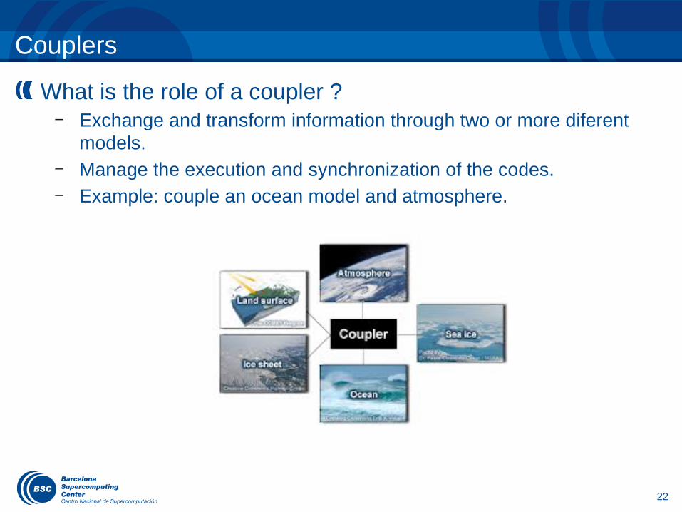
Post-processing

Once the model is run successfully, we need to post-process results to visualize data

– Maps– Plots– Text files– 3D Animations

24

Models at BSC

Mineral Dust Modeling– BSC-DREAM8b V2: Dust REgional Atmospheric

● Model● Fortran Code● Not parallel

NMMB/BSC-CTM– Meteorology-Chemistry coupled model

● Meteo. Driver: Nonhydrostatic Multiscale ● Model on the B grid (NMMB) ● Fortran Code● MPI

Climate Change– EC-EARTH

● Fortran, C● MPI, OpenMP

25

3D Outputs

Preprocess

Execution diagram: Focus on the Preprocessor

Tested in two cases: Global domain 1ºx1.4º resolution Global domain 12km x 12km

28

CompSs

COMPSs programming model intends to maximize the programmability of Java applications running on parallel and distributed infrastructures.

COMPSs is fully developed at BSC.

29

Original Preprocess

Preprocess is divided in two main tasks:– Fixed: which is only done once, when configuring the model– Variable: is done each run, as takes daily meteorological and surface

sea temperature inputs.– Fixed and Variable are now run separately.

Totally sequential, synchronous, ignore data dependencies between subprocesses.

#FIXED./exe/smmount.x./exe/landuse.x./exe/landusenew.x./exe/topo.x./exe/stdh.x./exe/envelope.x./exe/topsoiltype.x./exe/botsoiltype.x./exe/toposeamask.x./exe/stdhtopo.x./exe/deeptemperature.x./exe/snowalbedo.x./exe/vcgenerator.x./exe/roughness.x./exe/gfdlco2.x./exe/lookup_aerosol.x

#VARIABLEln -s ../meteo_data/wafs.00.0P5DEG.13042400.grib1 ../output/gfs.t00z.pgrb2f00ln -s ../meteo_data/sst2dvar_grb_0.5.13042400.grib1 ../output/sst2dvar_grb_0.5

./degribgfs_generic_05.sh 00 00 03 pgrb2f ../output

./exe/gfs2model_rrtm.exe 00

./exe/inc_rrtm.x

./exe/cnv_rrtm.x

./exe/degribsst.x

./exe/albedo.x

./exe/albedorrtm1deg.x

./exe/vegfrac.x

./exe/z0vegustar.x

./exe/allprep_rrtm.x

./exe/read_paul_source.x

./exe/dust_start.x

30

Original Performance

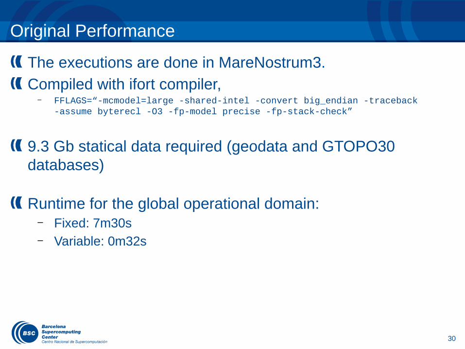
The executions are done in MareNostrum3.

Compiled with ifort compiler,– FFLAGS=“-mcmodel=large -shared-intel -convert big_endian -traceback

-assume byterecl -O3 -fp-model precise -fp-stack-check”

9.3 Gb statical data required (geodata and GTOPO30 databases)

Runtime for the global operational domain:– Fixed: 7m30s– Variable: 0m32s

31

Porting to COMPSs (I)

Preprocess is a collection of Fortran codes.

In order to port to COMPSs, we need to modify sources to manage files as arguments instead of being hardcoded.

Example: – smmount creates two files, seamaskDEM and heightDEM.– With COMPSs, smmount is executed with files as arguments

● ./smmount ../output/seamaskDEM ../output/heightDEM

Fortran source code is modified to handle arguments.

Each executable is wrapped in a Java method and selected as a task.

This method is not hard to code, but allprep executable in variable, manages more than 44 files !!!

32

Porting to COMPSs (II)

Then, three files are written in JAVA:– Fixed.java: main program of the application, contains task calls.– FixedBinaries.java: implementation of each task with the call to the

executable.– FixedItf.java: selection of tasks, providing the necessary metadata

about their parameters.

The same files are written for Variable.

33

Execution

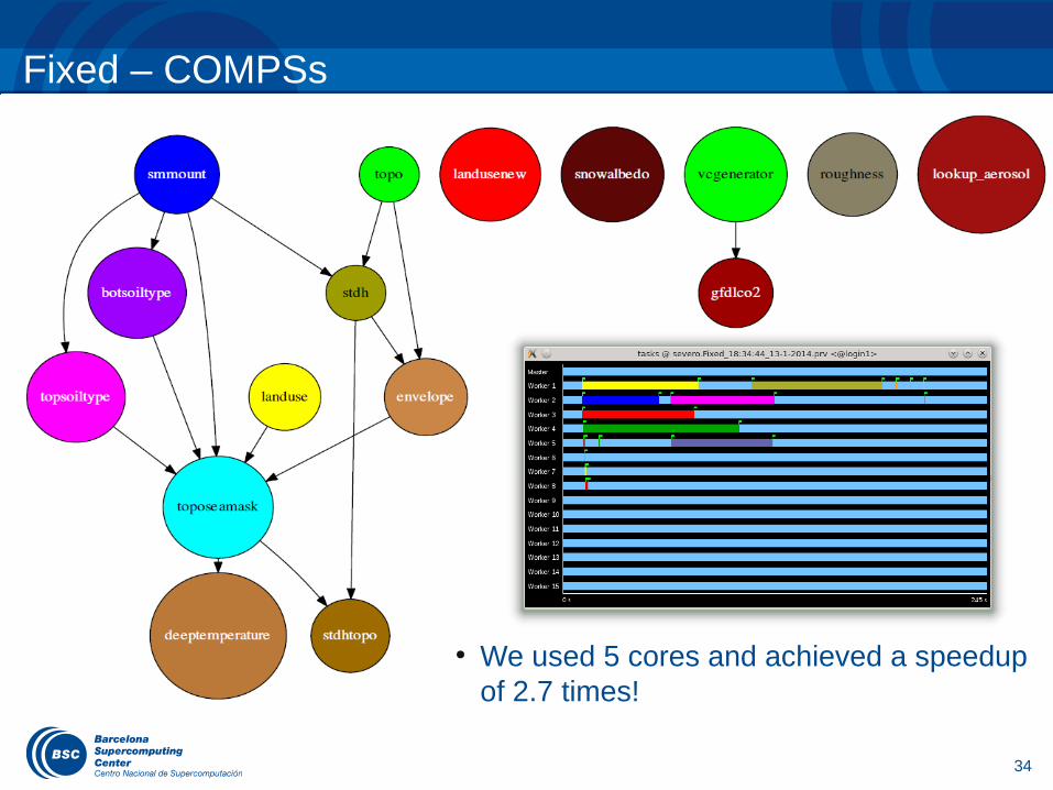
We implemented a Fortran/MPI application only for the Fixed preprocess, using 5 cores of one node based on the dependency graph acquired from CompSs.

Runtime for the global domain, 24 km:– Fixed: 2m30s.

Fixed – COMPSs

34

● We used 5 cores and achieved a speedup of 2.7 times!

Variable – COMPSs

35

The serial part allprep consumes a lot of time, we should investigate a hybrid solution because of memory issues

Need to be improved for higher resolution forecasts

36

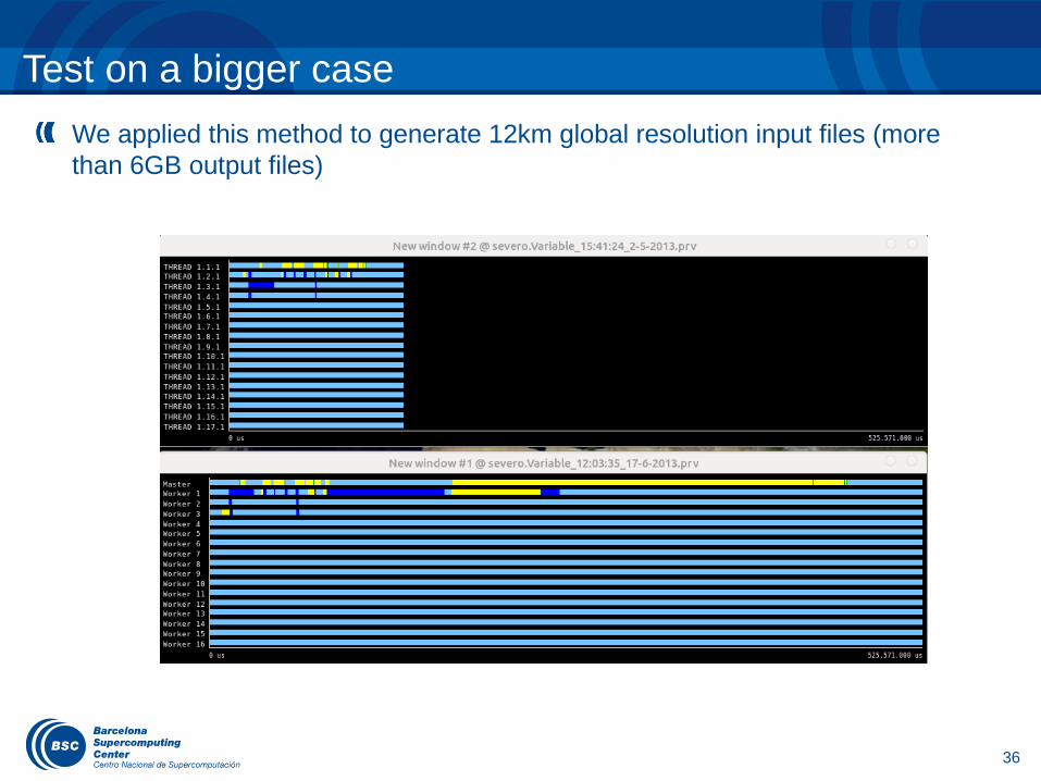
We applied this method to generate 12km global resolution input files (more than 6GB output files)

Test on a bigger case

37

Execution Remarks

Data dependencies between tasks are automatically detected, thus exploiting the inherent concurrency of the application when executing the tasks.

In the Fixed application, 8 tasks are free of dependencies at the beginning, and therefore they can be sent for execution immediately.

Performance– Fixed: the exploitation of task parallelism speeds up the process.– Variable: it has little computation and parallelism, which does not

compensate the overhead of task processing and distribution (e.g. dependency analysis, file transfer, task submission), hence incrementing the execution time.

Performance Analysis of NMMB/BSC-CTM Model

Execution diagram – Focus on the Model

Study domain: Global domain 24km x 24km resolution

Paraver

40

One hour simulation of NMMB

Last four processes are used for I/O

Paraver - Dimemas

41

It seems that previously there was noise during the execution

Issue with I/O

42

There is no parallel I/O implemented! Last hour

With I/O Without I/O

Issue with the last binary file

43

Last binary is written with delay.

Example regional 11km resolution

4778176548 Dec 15 09:25 nmmb_hst_01_bin_0000h_00m_00.00s 4778176548 Dec 15 09:28 nmmb_hst_01_bin_0001h_00m_00.00s 4778176548 Dec 15 09:31 nmmb_hst_01_bin_0002h_00m_00.00s 4778176548 Dec 15 09:34 nmmb_hst_01_bin_0003h_00m_00.00s 4778176548 Dec 15 09:38 nmmb_hst_01_bin_0004h_00m_00.00s 4778176548 Dec 15 09:41 nmmb_hst_01_bin_0005h_00m_00.00s 4778176548 Dec 15 10:42 nmmb_hst_01_bin_0006h_00m_00.00s

Issue with I/O – Mapping

44

Initial mapping for an experiment with 64 cores where the last 4 ranks are the write tasks

Final mapping

Issue with the last binary file solved

45

The instrumented execution has no issue…

4778176548 Dec 15 11:14 nmmb_hst_01_bin_0000h_00m_00.00s 4778176548 Dec 15 11:17 nmmb_hst_01_bin_0001h_00m_00.00s 4778176548 Dec 15 11:21 nmmb_hst_01_bin_0002h_00m_00.00s 4778176548 Dec 15 11:24 nmmb_hst_01_bin_0003h_00m_00.00s 4778176548 Dec 15 11:27 nmmb_hst_01_bin_0004h_00m_00.00s 4778176548 Dec 15 11:30 nmmb_hst_01_bin_0005h_00m_00.00s 4778176548 Dec 15 11:33 nmmb_hst_01_bin_0006h_00m_00.00s

Performance of different mapping and more I/O servers

46

The new mapping improved the execution time between 2.73 and 3.85 times

Processor Affinity

47

Processor affinity improved the execution time between 2.8% and 10% (some colleagues reported 20% improvement)

48

Decomposition (X,Y)

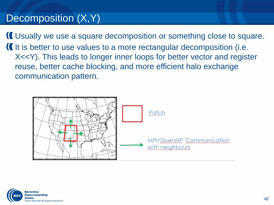
Usually we use a square decomposition or something close to square.

It is better to use values to a more rectangular decomposition (i.e. X<<Y). This leads to longer inner loops for better vector and register reuse, better cache blocking, and more efficient halo exchange communication pattern.

Decomposition

49

New decomposition improved the execution time till 6.5%

Throttling mechanism

An application is developed for many years and some times the scientists are not located anymore in the department

Use gprof (-pg) to figure out number of calls and duration of functions

Use Intel Fortran compiler with “-g -finstrument-functions” option and create a function list with the following rule, do not instrument the functions that are executed more than 10,000 times and the duration of each call is less than 1ms or 0%For example:00000000008c0230 # module_dynamics_routines_mp_hdiff_

Paraver

51

One hour simulation of NMMB, global, 24km, 64 layers

meteo: 9 tracers

meteo + aerosols: 9 + 16 tracers

meteo + aerosols + gases: 9 + 16 + 53

Paraver – Useful computation - Meteo

52

Paraver - Information about functions

53

One hour simulation of NMMB, global 24kmMeteo

Functions Percentage IPC

rrtm 13.7% - 52% (31.3%)

2.18 - 2.38

gather_layers

8.26% - 13.7% (11.1%)

X

scatter_layers

10.6% - 14.1% (12.1%)

X

Meteo + aerosols + chemistry


run_ebi 14% - 20.3% (16.55%)

0.71-1.11

rrtm 3.97% - 15.07% (9.05%)

2.17 – 2.37

gather_layers

12.37% - 24.55% (16.93%)

X

scatter_layers

14.65% - 26.58% (19%)

XMeteo +

aerosols


rrtm 8.8% - 33.4% (20.33%)

2.2 – 2.4

gather_layers 11.9% - 22% (17.4%)

x

scatter_layers 14.4% - 26.6% (19.5%)

X

Paraver – Global – 24km - Meteo

Simulation: 02/12/2005

Paraver – Global – 24km – Meteo – between radiations

Paraver – Global – 24km – Meteo – radiation

Communication matrix

Paraver – Global – 24km – Meteo/Dust/Chem


Paraver – Global – 24km – Meteo/Dust/Chem


Paraver – (useful) user functions

Paraver – (useful) user functions

Computation load impalance

Tracer Monotonization

This routine is designed with a not efficient approach, the serialization can be observed

Zoom between radiation calls for dust/sea-salt

Polar filters

The execution time with 65 cores is increased by 60% at least (without I/O) but the functions gather/scatter are improved by 5.2 - 5.8 times.

0 500 1000 1500 2000 25000

2

4

6

8

10

12

14

Speedup

Number of cores

Sp

eedu

p

Speedup – Global 24km – 64 layers

For the extra datapoint we use a domain of 16 x 128 processors instead of 32 x 64

Code vectorization

MUST - MPI run time error detection

OmpSs Programming Model

OmpSs Introduction

Parallel Programming Model - Build on existing standard: OpenMP

- Directive based to keep a serial version - Targeting: SMP, clusters, and accelerator devices

- Developed in Barcelona Supercomputing Center (BSC) Mercurium source-to-source compiler

Nanos++ runtime system

OmpSs Example

72

Roadmap to OmpSs

NMMB is based on the Earth System Modeling Framework (ESMF)

The current ESMF release (v3.1) is not supporting threads. However, the development version of NMMB uses ESMF v6.3

Post-process broke because of some other issues but it was fixed

The new version of NMMB with OmpSs support has been compiled and is ready to apply and test OmpSs

Current work to be presented at PRACE Scientific and Industrial Conference 2014

73

Improved I/O (future work)

Parallel NetCDF written to single files by all MPI tasks.

74

Future workUse OmpSs programming model● Study GPU case● Explore Xeon Phi

Prepare NMMB model for higher resolutions, first milestone is the global model for 12km

Improve performance and scale NMMB for thousands of cores

Fix I/O issue - IS-ENES Exascale Technologies & Innovation in HPC for Climate Models workshop - Possible collaboration across the community to focus on a global solution

Data Assimilation

Data Assimilation – Motivations

Dust optical depth: 2014 01 06 h+00

http://sds-was.aemet.es/forecast-products/ dust-forecasts/compared-dust-forecasts

Atmospheric models are far from being perfect A considerable amount of accurate earth observations is available

Data assimilation 'optimally' combines models and observations

http://www.wmo.int/pages/prog/gcos/

77

Data Assimilation – WorkflowEnsemble background

Ensemble analysis

Observations

Ensemble background

Mean analysis

Kalman filter*short-term

forecast

long-term

forecast

http://aeronet.gsfc.nasa.gov/

http://modis-atmos.gsfc.nasa.gov/

* In collaboration with N. Schutgens (Uni. Oxford, UK)

Data Assimilation – Workflow

http://modis-atmos.gsfc.nasa.gov/

BASH script starts the submission of the assimilation job● We want all the ensembles to be executed in parallel● We have 40 ensembles, we provide 20 cores for each execution and one

ensemble for long-forecast. We should need totally 82 nodes (1,312 exclusive cores)

● Now, we need 52 nodes (832 cores), ~36% less resources

www.bsc.es

Thank you!

For further information please [email protected]

79

Documents

Performance Analysis of an Earth Science Application