Performance Analysis of CR-honeynet to preventJamming Attack through Stochastic Modeling I

Suman Bhuniaa, Shamik Senguptaa, Felisa Vazquez-Abadb

aDept. of Computer Science and Engineering, University of Nevada, Reno, USA 89557bDept. of Computer Science, Hunter College, City University of New York, USA 10065

Abstract

Cognitive Radio Network (CRN) has to stall its packet transmission periodicallyto sense the spectrum for Primary User’s (PU’s) transmission. The limited anddynamically available spectrum and fixed periodic schedule of transmission in-terruption makes it harder to model the performance of a CRNs. Again, anopen and dynamic spectrum access model brings forth a serious challenge ofsustenance among the CRN and makes them more susceptible to jamming-based denial of service (DoS) attacks. Inspired by honeypot in the networksecurity, we propose a honeynet based defense mechanism called CR-honeynet.CR-honeynet aims to avoid attacks on legitimate communications by dedicatinga Secondary User (SU) as a honeynode, to deter the attacker from attackinglegitimate SUs and attack the honeynode instead. Dedicating an SU as hon-eynode, on account of its permanent idleness, is wasteful of an entire node asa resource. We seek to resolve the dilemma by dynamically selecting the hon-eynode for each transmission period. The contribution of the current paper istwo-fold. Initially, we develop the first comprehensive queuing model for CRNs,which pose unique modeling challenges, due to their fixed periodic sensing andtransmission cycles. In the second step, we introduce a series of strategies forhoneynode selection to combat these attacks while keeping the CRN’s perfor-mance optimal for different traffic scenarios. We build a simulation of a CRNunder jamming attack and analyze its performance with different honeynodeselection strategies. We find that the predictions, of our mathematical model,track closely with the results of our simulation experiments.

Keywords: Cognitive Radio, Jamming attack, Honeynet, Stochastic Model,Queuing theory, queue with vacation

IThis research was supported by NSF CAREER grant CNS #1346600.Email addresses: sumanbhunia@gmail.com (Suman Bhunia), felisav@hunter.cuny.edu

(Felisa Vazquez-Abad)URL: http://www.cse.unr.edu/~shamik (Shamik Sengupta)

Preprint submitted to Pervasive and Mobile Computing February 1, 2015

1. Introduction

The conventional static spectrum allocation policy has resulted in subop-timal use of spectrum resource, leading to over-utilization in some bands andunder-utilization in others [1]. As a solution, dynamic spectrum access-basedCognitive Radio (CR) has been proposed. CR allows secondary users (SUs) touse an idle licensed spectrum while the proprietary primary user (PU) is nottransmitting. The IEEE 802.22 [2] which is an emerging standard for CR-basedwireless regional area networks (WRANs), aims at a vacant licensed TV spec-trum to be used by SU without causing interference to PU. Infrastructure-basedcognitive radio networks (CRNs) consist of two major components: a centralcontroller (such as base station or access point) and mobile SUs. The centralcontroller supervises the communication and makes the spectrum allocation de-cisions. A sample CRN is presented in Fig. 1.

Figure 1: A sample CRN with an at-tacker

The dynamic nature of the available spec-trum makes CRNs vulnerable to several spec-trum etiquette attacks. The IEEE 802.22standard does not specifically address the SU-SU interaction or SU protection, although itproactively specifies the PU protection. The“open” philosophy of the CR paradigm makessuch networks susceptible to attacks by smartmalicious users that could even render the le-gitimate CR spectrum-less [1, 3, 4]. Due tosoftware reconfigurability, CRs can even bemanipulated to disrupt other CRNs or legacywireless networks with even greater impact than traditional hardware radios.The jamming-based Denial of Service (DoS) [1] attack is achieved by transmit-ting energy on the channel where a legitimate SU is communicating. An attackercan scan through channels, identify ongoing legitimate SU communication andthen transmit a jamming signal on that particular channel causing heavy inter-ference to the SU, which in effect, can block the legitimate SU’s transmissioncompletely.

A number of defense mechanisms against such attacks have been attempted[5–10]. Most of these techniques have considered that the attacker is naiveand does not evolve. Inspired by “honeypot” in cybercrime, we propose CR-honeynet, which passively learns the attacker’s strategy of assault and thendedicates an SU as an active decoy to lure the attacker to hit the decoy node.In this way, the assailant gets false satisfaction of attack, while legitimate SUsbypass attacks. In our earlier paper [11], We introduced the learning mechanismof CR-Honeynet. However the effectiveness of CR-Honeynet in CRN has to bestudied before a CRN can deploy CR-Honeynet mechanism. The goal of thispaper is to investigate whether allocating resources for CR-honeynet can bebeneficial for improving system performance.

To protect PU incumbent services, DSA strictly enforces SUs to periodicallypause its transmission and sense for PU activity. SUs scan the wireless envi-

2

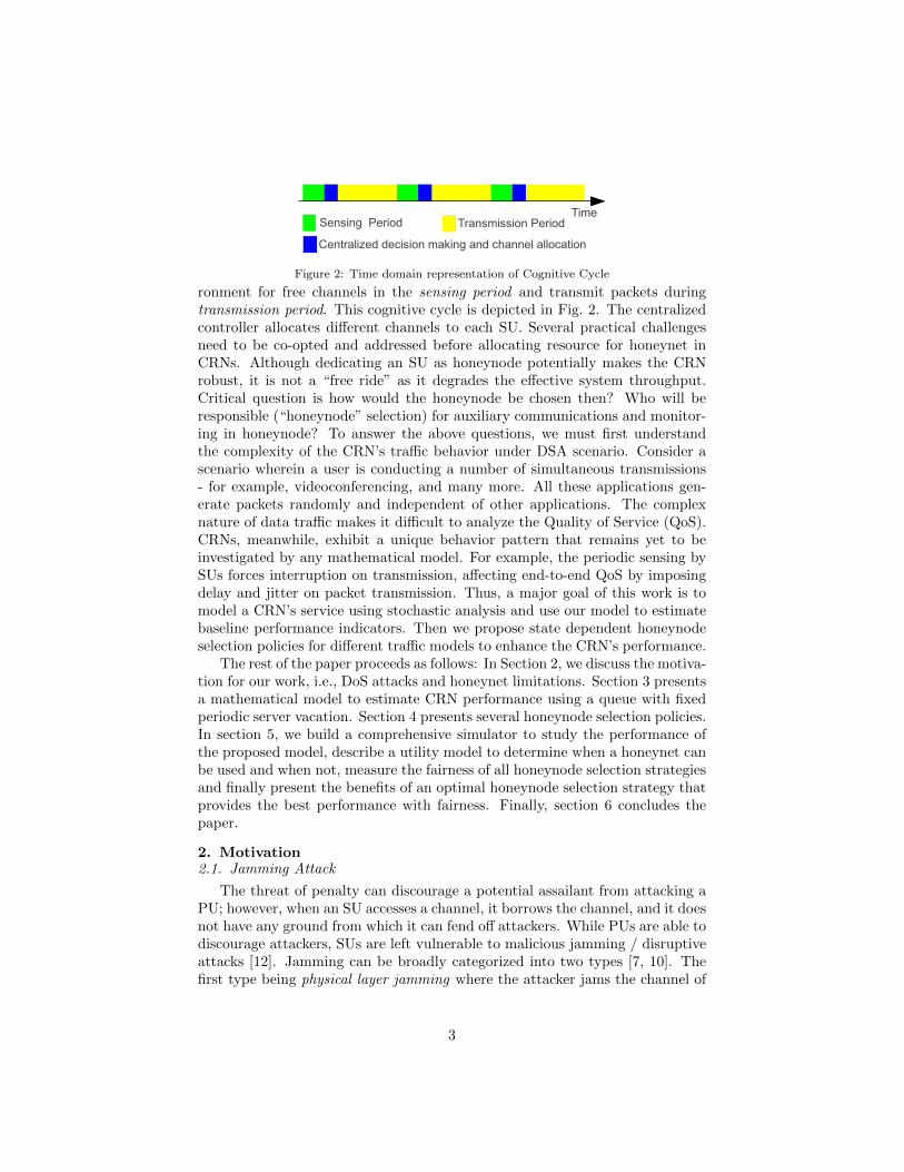
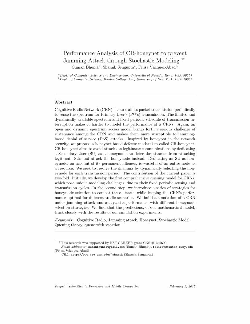
Figure 2: Time domain representation of Cognitive Cycle

ronment for free channels in the sensing period and transmit packets duringtransmission period. This cognitive cycle is depicted in Fig. 2. The centralizedcontroller allocates different channels to each SU. Several practical challengesneed to be co-opted and addressed before allocating resource for honeynet inCRNs. Although dedicating an SU as honeynode potentially makes the CRNrobust, it is not a “free ride” as it degrades the effective system throughput.Critical question is how would the honeynode be chosen then? Who will beresponsible (“honeynode” selection) for auxiliary communications and monitor-ing in honeynode? To answer the above questions, we must first understandthe complexity of the CRN’s traffic behavior under DSA scenario. Consider ascenario wherein a user is conducting a number of simultaneous transmissions- for example, videoconferencing, and many more. All these applications gen-erate packets randomly and independent of other applications. The complexnature of data traffic makes it difficult to analyze the Quality of Service (QoS).CRNs, meanwhile, exhibit a unique behavior pattern that remains yet to beinvestigated by any mathematical model. For example, the periodic sensing bySUs forces interruption on transmission, affecting end-to-end QoS by imposingdelay and jitter on packet transmission. Thus, a major goal of this work is tomodel a CRN’s service using stochastic analysis and use our model to estimatebaseline performance indicators. Then we propose state dependent honeynodeselection policies for different traffic models to enhance the CRN’s performance.

The rest of the paper proceeds as follows: In Section 2, we discuss the motiva-tion for our work, i.e., DoS attacks and honeynet limitations. Section 3 presentsa mathematical model to estimate CRN performance using a queue with fixedperiodic server vacation. Section 4 presents several honeynode selection policies.In section 5, we build a comprehensive simulator to study the performance ofthe proposed model, describe a utility model to determine when a honeynet canbe used and when not, measure the fairness of all honeynode selection strategiesand finally present the benefits of an optimal honeynode selection strategy thatprovides the best performance with fairness. Finally, section 6 concludes thepaper.

2. Motivation2.1. Jamming Attack

The threat of penalty can discourage a potential assailant from attacking aPU; however, when an SU accesses a channel, it borrows the channel, and it doesnot have any ground from which it can fend off attackers. While PUs are able todiscourage attackers, SUs are left vulnerable to malicious jamming / disruptiveattacks [12]. Jamming can be broadly categorized into two types [7, 10]. Thefirst type being physical layer jamming where the attacker jams the channel of

3

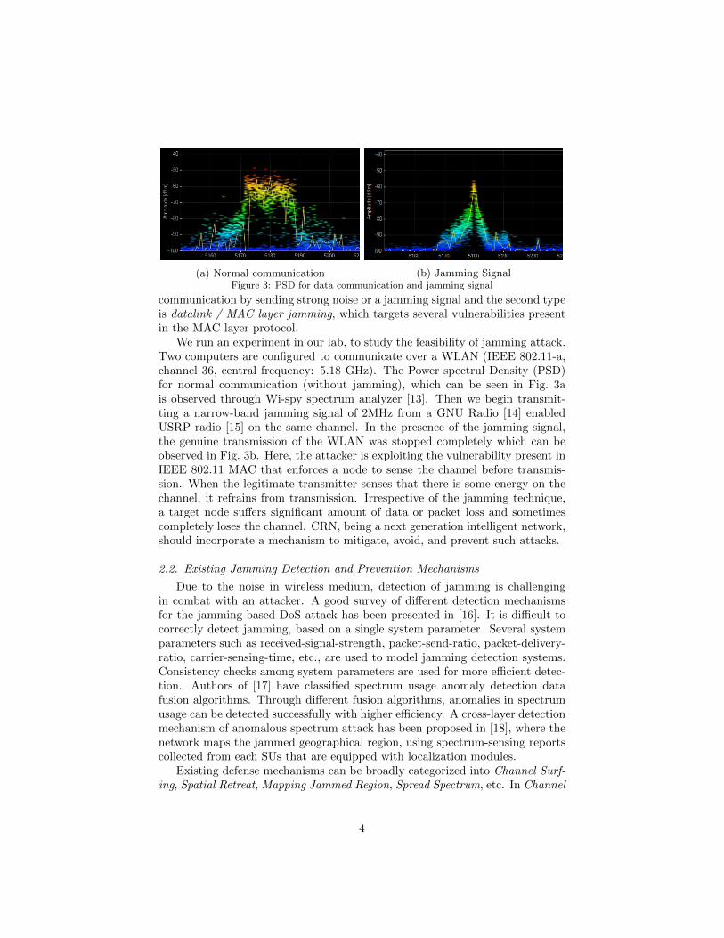
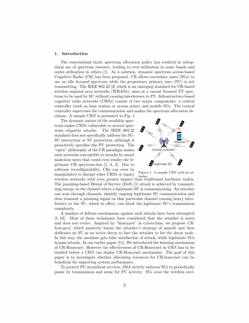
(a) Normal communication (b) Jamming SignalFigure 3: PSD for data communication and jamming signal

communication by sending strong noise or a jamming signal and the second typeis datalink / MAC layer jamming, which targets several vulnerabilities presentin the MAC layer protocol.

We run an experiment in our lab, to study the feasibility of jamming attack.Two computers are configured to communicate over a WLAN (IEEE 802.11-a,channel 36, central frequency: 5.18 GHz). The Power spectrul Density (PSD)for normal communication (without jamming), which can be seen in Fig. 3ais observed through Wi-spy spectrum analyzer [13]. Then we begin transmit-ting a narrow-band jamming signal of 2MHz from a GNU Radio [14] enabledUSRP radio [15] on the same channel. In the presence of the jamming signal,the genuine transmission of the WLAN was stopped completely which can beobserved in Fig. 3b. Here, the attacker is exploiting the vulnerability present inIEEE 802.11 MAC that enforces a node to sense the channel before transmis-sion. When the legitimate transmitter senses that there is some energy on thechannel, it refrains from transmission. Irrespective of the jamming technique,a target node suffers significant amount of data or packet loss and sometimescompletely loses the channel. CRN, being a next generation intelligent network,should incorporate a mechanism to mitigate, avoid, and prevent such attacks.

2.2. Existing Jamming Detection and Prevention Mechanisms

Due to the noise in wireless medium, detection of jamming is challengingin combat with an attacker. A good survey of different detection mechanismsfor the jamming-based DoS attack has been presented in [16]. It is difficult tocorrectly detect jamming, based on a single system parameter. Several systemparameters such as received-signal-strength, packet-send-ratio, packet-delivery-ratio, carrier-sensing-time, etc., are used to model jamming detection systems.Consistency checks among system parameters are used for more efficient detec-tion. Authors of [17] have classified spectrum usage anomaly detection datafusion algorithms. Through different fusion algorithms, anomalies in spectrumusage can be detected successfully with higher efficiency. A cross-layer detectionmechanism of anomalous spectrum attack has been proposed in [18], where thenetwork maps the jammed geographical region, using spectrum-sensing reportscollected from each SUs that are equipped with localization modules.

Existing defense mechanisms can be broadly categorized into Channel Surf-ing, Spatial Retreat, Mapping Jammed Region, Spread Spectrum, etc. In Channel

4

Surfing technique, the node which is under attack, migrates its channel of com-munication upon detection of jamming [5]. Authors of [6] proposed proactivefrequency hopping, where the nodes change its channel of communication, irre-spective of attacks to avoid jamming. The authors considered a fixed numberof channels that the attacker can use, that is known to an SU, which in realityis difficult to achieve. In Spatial Retreat [7], mobile nodes relocate themselvesphysically to avoid jamming. The constraint of this approach is that the nodesare required to be highly mobile, which is not applicable for static nodes. InMapping Jammed Region [8] approach, the multi-hop, and intensely populated,CRN avoids routing through the links that have been affected by jamming. Thismechanism fails if there is only one path and that path is attacked. Majorityof current countermeasures defend against jamming after it has been detected;on the contrary, CR-Honeynet learns from the history of attack and provideproactive defense mechanism.

2.3. Use of Honeynet in avoiding attacks

“Honeypot,” in cybercrime, is defined as “a security resource who’s value liesin being probed, attacked or compromised”. In cybercrime defense, honeypotsare being used as a camouflaging security tool with little or no actual produc-tion value to lure the attacker into giving them a false sense of satisfaction, thusbypassing (reducing) the attack impact and giving the defender a chance to re-trieve valuable information about the attacker and their activities. This node iscalled honeynode. A single channel honeypot-based channel surfing, to mitigatejamming-based DoS attacks, has been proposed in [10]. The network dedicatesa node, as honeypot, to monitor attacks. Upon detection of attack, the networkswitches its channel of operation, which results in long-time communication dis-ruption. Majority of the previous works have assumed that the attacker is naiveand does not evolve. Thus, none of these works have focused on learning thestrategy of attacker where the attacker is also dynamic and changes its strategyof choosing the target communication characteristics.

From an intelligent and rational attacker’s perspective, jamming a commu-nication randomly will not yield optimal results; rather, an attacker can bemost disruptive if it targets the communication that impacts the CRN mostseverely upon interruption [16, 19–21]. The attacker succeeds in determininghighest impacting communication by observing certain transmission character-istics, for example, highest transmission power, highest data rate, modulationscheme, packet inter arrival time, quality of route with end-to-end acknowledg-ments, etc. [16]. To proactively defend against such intelligent attackers, a CRNmust learn about the strategy that the attacker uses, to figure out the highestimpacting communication. The attacker’s strategy of finding the highest im-pacting communication can be used as a trap by the defending CRN to detractthe attacker from striking legitimate communications.

We propose CR-honeynet, a honeynet-based defense mechanism where theCRN passively learns the strategy of the attacker and then places an activedecoy, namely honeynode to entice the attacker for jamming the honeynodetransmission. Thus, the attacker gets a false impression of attacking the highest

5

impacting communication, whereas legitimate SU communications avoid attacksand reduce attack impact on the CRN. The SU, acting as honeynode, refrainsfrom transmitting its own data packets and instead transmits garbage data withspecific transmission characteristics. Such transmission characteristics lure theattacker to jam the honeynode’s transmission. For example, if an attacker tar-gets the highest transmission power, then the honeynode transmits with highestpossible power, while all other SUs keep their transmission power lower thanthe honeynode’s power.

The description of the learning mechanism of honeynet is provided in [11].When CR-honeynet is deployed, and the attacker is evolving, the attacks willsometimes be trapped by honeynode, and sometimes can strike legitimate SUs.We define one parameter, attractiveness of honeynet (ξ) as the probability thatthe honeynode is the one to be attacked, conditional on observing a jammingattack. Note that ξ depends on how well the CR-honeynet learning mechanismworks. In this paper, our goal is to investigate the effectiveness of CR-honeynetwith different values of ξ and determine when it is/not beneficial to deployCR-honeynet.

2.4. Queue model

Honeynode ensures less data loss at the cost of end-to-end delay. Some ap-plication can tolerate data loss but not delay and others the opposite. The goalis to build a mathematical model that can estimate system performance beforewe actually deploy CR-honeynet. If honeynode assignment results in degrada-tion of overall system performance then we can opt for not assigning honeynet.The end-to-end delay in CR is mainly affected by queuing delay as processing,transmission and propagation delays are negligible compared to queuing delay.Our theoretical model focus on determining queuing delay. Then we concentrateon honeynode selection strategies to achieve better over-all system performance.

We can model an SU as a server with vacation where vacation is specialservice with higher priority. There are many mathematical models that dealswith servers with vacations [22–25] where the server has the option to takevacations only at the end of its current service. Because the sensing period hasdeterministic length and intervals, the server model does not conform to theusual server with vacations. Instead, the sensing period acts as a “priority”customer whose inter-arrival rates and service times are deterministic. In thiscase a packet transmission has to be delayed if this packet can not be transmittedwithin the transmission period. In this paper we derive a mathematical modelfor server with deterministic vacations that portray the behavior of SUs in CR-Honeynet.

3. Mathematical Model of an SU3.1. Queuing Characteristics

In earlier telecommunication networks, voice packets were generated at fixedrates or at fixed burst sizes [26, 27]. For this kind of system the inter-arrival timeis fixed and the value depends on the codec (voice digitization technique) used

6

[26, 27]. Voice activity detection and Silence suppression techniques introducesrandomness in packet arrival time.

Figure 4: Depiction of how packets arrive toqueue

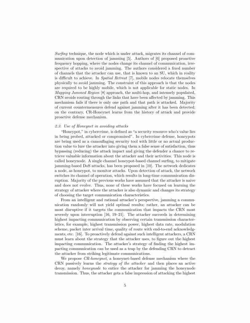
With the increase in usage of mul-timedia applications on smart-phonesthe nature of the traffic flow is verycomplex to model. Because of the in-dependence between sources, a mem-oryless inter-arrival time may be agood model. This observation is sup-ported by statistical analysis. Thestudies carried out in various exper-iments [28–31] have concluded thatwhen many different applications aremerged, the packet arrival process tends to follow Poisson process. Fig. 4 pro-vides a depiction of how packets from different applications flow to a queue. Weuse λi to denote the rate of the Poisson process of packet arrivals at SU labeledi, and {Ni(t); t ≥ 0} to denote the corresponding arrival process. When a singlequeue is analyzed, we drop the subindex i.

Each SU is modeled as a FCFS (first come-first served) queue with oneserver. Packets arrive according to a marked Poisson process with rate λ and“marks” specifying the packet size in number of bytes. In our model, the marks{Y1, Y2, . . .} are independent and identically distributed uniform random vari-ables. The aggregate byte arrival rate is thus λE(Y ). Each SU can transmit ata fixed data transmission rate. Therefore, the service time of a packet of sizeYn is, Sn = (Yn/data rate) and it has uniform distribution U(`1, `2), with meanE(S) = (`1 + `2)/2 and maximal service rate, µ = 1/E(S).

During the transmission periods of length Tt, the model corresponds to aM/G/1 queue [23] where the service time of consecutive packets {Sn} are in-dependent and identically distributed. During the sensing periods of length Tsand transmission periods when the SU is chosen as a honeynode our server stopsservicing the queue, which nonetheless continues to accumulate arriving pack-ets. The effect of an attack during a transmission period when the SU is not ahoneynode is that all packets transmitted in that slot are lost.

The two performance criteria of interest are the (stationary) average waitingtime in queue per packet (Wq), and the average packet drop rate (pdr). In thecase of infinite buffer pdri is also the long term probability that the i-th SU isattacked, that we call θi.

3.2. Queuing Model with Vacations

For simplicity, we assume that there are more free channels than the numberof SUs in the CRN. In this section we assume that an SU is chosen to be“sacrificed” as a honeynode at every transmission period. If an SU is chosen asa honeynode, then all the new arriving packets join the queue and wait untilthe next transmission period, where the SU is not chosen as a honeynode. Theanalysis of this section assumes a random policy, where the i-th SU is chosenas honeynode with probability pi, independently of past assignments and of

7

the state of the CRN. Other benchmark policies (such as round robin) will bediscussed in later sections and compared via simulation experiments.

The amount of service time that must be postponed at the start of a sensingperiod is either 0 (when the server is idle at time of sensing) or it has the valueof the random variable S representing the fraction of service time that must bepostponed. In steady state, if ρ = P(the server is busy) then the server is notidle with probability ρ. Thus, calling X the fraction of service that must bepostponed, we have:

X =

{0 w.p. 1− ρS w.p. ρ

We now characterize the random variable S, Condition on the event thatthe sensing period starts when the queue is still not empty. When transmissionstarts, consecutive service times S1, S2, . . . accumulate until the last service thatdoes not fit into transmission. We now provide precise definitions and results.Let M(t) = min(n : S1 + . . .+Sn ≤ t). This is a renewal process and it indicatesthe times of start of successive service epochs. Call

Jn =

n∑j=1

Sj ,

then for time t = Tt we are interested in what is known as the “age” or “back-ward recurrence time” of the renewal process M(t) at time t = Tt:

S = Tt − JN(Tt).

For a renewal process with no preemption, the distribution of this variableand its expectation can be calculated asymptotically [23]. In our model, where“many” services can be completed during transmission time (specifically, when`2 << Tt) we can argue that S will have this known asymptotic distribution asan approximate distribution, so that

P(S ≤ x) =1

E(S)

∫ x

0

(1− F (u)) du

where F (u) is the distribution corresponding to the uniform random variable Sbetween `1 and `2.

Lemma 1. Assume that P(S ≤ x) = 1E(S)

∫ x0P(S > u) du. Then

E(S) =E(S2)

2E(S); E(S2) =

E(S3)

3E(S).

Proof. Let g be any differentiable function with bounded derivative. Callf(·) the density of the service time S. Using calculus it is straightforward to

8

calculate:∫ ∞0

g′(x)P(S > x) dx =

∫ ∞0

g′(x)

∫ ∞x

f(y) dy =

∫ ∞0

dy

(∫ y

0

g′(x) dx

)f(y)

=

∫ ∞0

g(y)f(y)− g(0) = E(g(S))− g(0).

Thus, using g(x) = x2/(2E(S)) we obtain the result for E(S) and using g(x) =x3/(3E(S)) we obtain the result for E(S3). �

Using this approximation,

E(X) =ρE(S2)

2E(S)(1)

For any constant a > 0,

E(a+X2) = ρ(E(a+ S)2 + (1− ρ)a2

= ρ(a2 + 2aE(S) + E(S2)) + (1− ρ)a2

= a2 + 2aE(S) + E(S2)

which yields:

E(a+X2) = a2 + aE(S2)

E(S)+

E(S3)

3E(S). (2)

We now calculate the effective utilization factor for the queue under therandom policy. Assuming that the queues are stable, the effective service ratefor each of the SUs satisfies the equation:

µ′i = µ

(Tt − ρi E(S)

Ts + Tt

)(1− pi), ρi =

λiµ′i,

which yields an implicit equation for µ′:

µ′i(Tt + Ts) = µ

(µTt −

E(S2)λi2E(S)µ′i

)(1− pi) (3)

Solving the quadratic equation (3) gives values of µ′i that depend on λi.

Remark: If all SUs have equal probability of being chosen (pi), then the re-duced service rate is the same as in the round robin policy.

Stationary policies. We now provide an analysis of the stationary queu-ing delay for the random (or round robin) policies. The analysis is done for eachqueue, and the subscript i will be dropped from our notation.

9

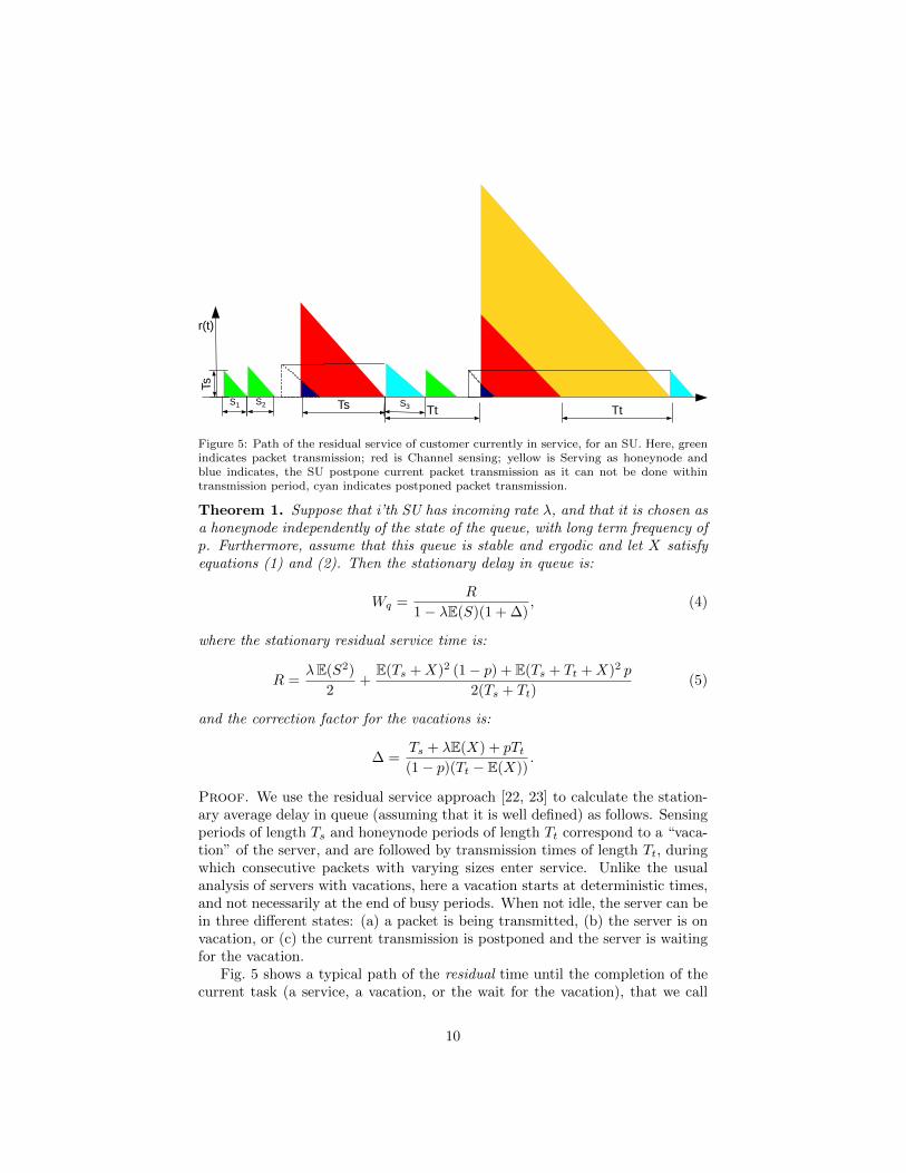
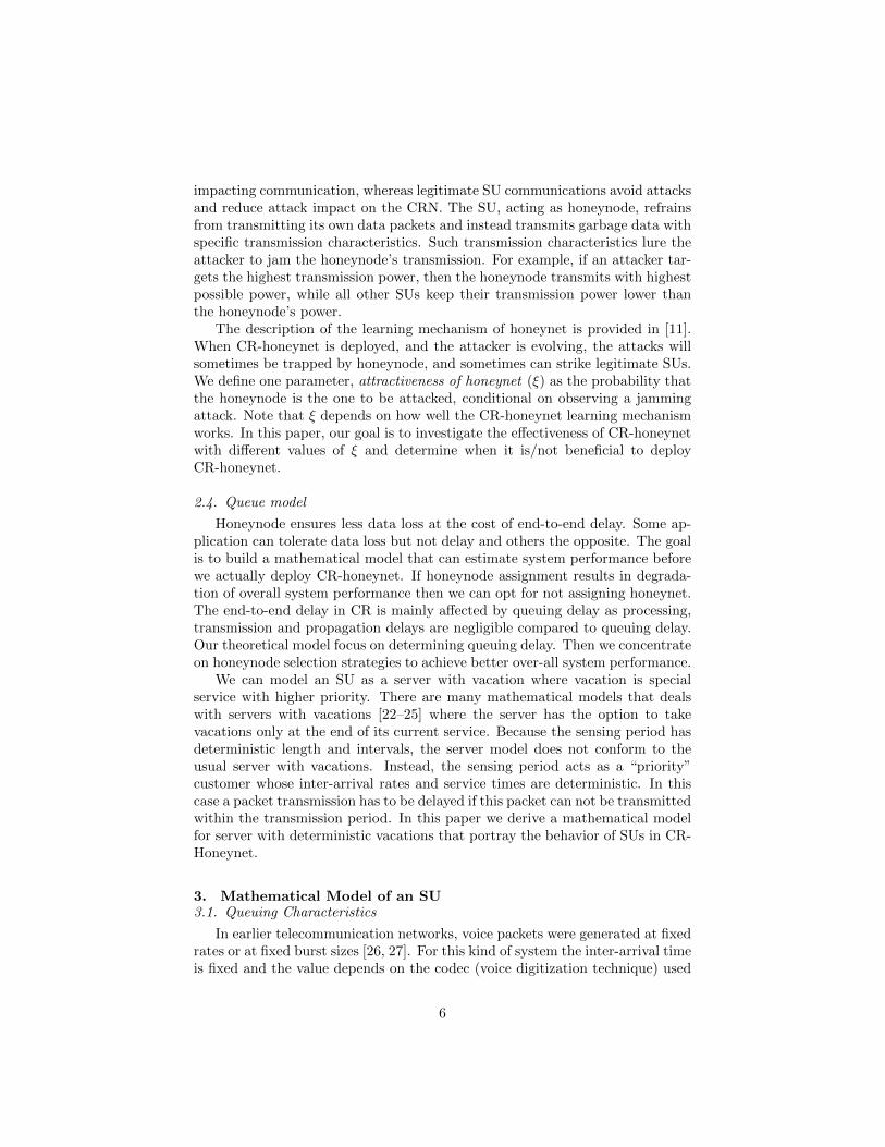
Figure 5: Path of the residual service of customer currently in service, for an SU. Here, greenindicates packet transmission; red is Channel sensing; yellow is Serving as honeynode andblue indicates, the SU postpone current packet transmission as it can not be done withintransmission period, cyan indicates postponed packet transmission.

Theorem 1. Suppose that i’th SU has incoming rate λ, and that it is chosen asa honeynode independently of the state of the queue, with long term frequency ofp. Furthermore, assume that this queue is stable and ergodic and let X satisfyequations (1) and (2). Then the stationary delay in queue is:

Wq =R

1− λE(S)(1 + ∆), (4)

where the stationary residual service time is:

R =λE(S2)

2+

E(Ts +X)2 (1− p) + E(Ts + Tt +X)2 p

2(Ts + Tt)(5)

and the correction factor for the vacations is:

∆ =Ts + λE(X) + pTt(1− p)(Tt − E(X))

.

Proof. We use the residual service approach [22, 23] to calculate the station-ary average delay in queue (assuming that it is well defined) as follows. Sensingperiods of length Ts and honeynode periods of length Tt correspond to a “vaca-tion” of the server, and are followed by transmission times of length Tt, duringwhich consecutive packets with varying sizes enter service. Unlike the usualanalysis of servers with vacations, here a vacation starts at deterministic times,and not necessarily at the end of busy periods. When not idle, the server can bein three different states: (a) a packet is being transmitted, (b) the server is onvacation, or (c) the current transmission is postponed and the server is waitingfor the vacation.

Fig. 5 shows a typical path of the residual time until the completion of thecurrent task (a service, a vacation, or the wait for the vacation), that we call

10

r(t). Under ergodicity, the stationary average residual service is the same as thelong term average, given by:

R = limt→∞

1

t

∫ t

0

r(t) dt = limt→∞

1

t

M(t)∑i=1

S2i

2+

V (t)∑i=1

L2i

2

(6)

where M(t) is the number of arrivals that have entered service up to time t, V (t)is the number of sensing periods up to time t, and Li is the length of the i-thvacation. It follows that Li are independent and identically distributed (iid)random variables random variables with composite distribution: with probabil-ity 1− p the vacation length is Ts +X, and with probability p it is Ts +Tt +X.For k ≥ 1, let

τk = min(t > τk−1 : Q(t) = 0); τ0 ≡ 0

be the consecutive moments when the queue empties. The stability assumptionimplies that the queue empties infinitely often (that is, the state Q = 0 ispositive recurrent), so that τk → +∞ with probability one. At these times,M(τn) = N(τn), and N(t)/t → λ, because N(·) is a Poisson process. Becausethe limit R (assuming that it exists) is the same if we consider any divergentsubsequence, we can take the limit along the subsequence {τk; k ≥ 0}. In ourmodel V (t)/t→ (Ts+Tt)

−1. Under ergodicity, long term averages are stationaryaverages, and

E(L2i ) = E(Ts +X)2(1− p) + E(Ts + Tt +X)2 p,

where X satisfies (1) and (2). Applying these results in (6) gives expression (5).The rest of the argument is as follows. It is a known property of Poisson

processes that sampling a system at Poisson arrival epochs yields states thathave a stationary distribution. This is sometimes called “ a random snapshot”of the system. In queuing theory this property is also known as “PASTA”(Poisson arrivals see time averages). Using this property an arriving customerwill encounter Nq customers in queue, where Nq is a random variable that hasthe stationary distribution of the queue length. The average wait time is thusthe sum of the expected service time of the Nq customers in queue, plus R, plusthe contribution of the vacation periods during the waiting time. Call T therequired service time for the customers in queue, then using Little’s Law:

E(T ) = E

Nq∑k=1

Sk

= E(NqE(S)) = λWqE(S).

Therefore, the stationary delay upon arrival at the queue will satisfy:

Wq = λWqE(S) +R+ vs(Ts + E(X)) + vh Tt, (7)

where vs and vh are the (expected) number of sensing and honeynode periods(respectively) that fall within the time required to transmit all the Nq customers

11

in front of the new arrival. In the expression above we have used the fact thatfor every sensing period, the actual vacation time is not just Ts but we must addthe lost time from the postponed service (if any). On average, the stationarycontribution of this excess is E(X).

We now proceed to the calculation of vs and vh. In order to do so, we willuse Wald’s theorem [23]. Given T , the actual number of (true) transmissionperiods required to provide the service for the Nq customers in queue is:

νt = min

(n :

n∑i=1

(Tt −Xi) ≥ T

), (8)

where Xi is the fraction of postponed service at the i-th sensing period. This isa stopping time adapted to the filtration Fn generated by {Zi ≡ Tt−Xi, i ≤ n}.In addition, Zn is independent of Fn−1. For our model the random variables{Zn} are bounded, thus absolutely integrable. It is straightforward to verifythat E(Xn1{νt<n}) = P(νt < n)E(X), and finally, E(νt) < ∞, which followsbecause νt ≤ T/(Tt−`2) w.p.1. Under these conditions, Wald’s Theorem ensuresthat

E

(νt∑i=1

Zi

)= E(νt)(Tt − E(X)).

Rewrite (8) as:∑νti=1 Zi ≤ T <

∑νt+1i=1 Zi and take expectations to get:

E(T )

Tt − E(X)− 1 < E(νt) ≤

E(T )

Tt − E(X).

In stationary state, we use the approximation E(νt) = λWqE(S)/(Tt−E(X)). Inorder to calculate vs and vh we reason as follows: given the number of honeyn-ode periods, the number of sensing periods is the number of true transmissionperiods required to exhaust the time T , plus vh, that is:

vs = E(νt) + vh = E(νt) + pvs, =⇒ vs =E(νt)

1− p.

Replacing now these values in (7) and using E(T ) = λWqE(S), we obtain

Wq = λWq E(S)

(1 +

Ts + E(X)

(1− p)(Tt − E(X))+ p

Tt(1− p)(Tt − E(X))

)+R,

which yields (4), after some simple algebra.

4. Honeynode Selection Policies

4.1. State Dependent Policies for Uniform traffic distribution

When an SU is chosen as honeynode with initial queue size of Q packets,the queue size at the beginning of the following transmission period is Q + A,

12

where A ∼ Poisson(λ(Ts+Tt)). In order to understand the effects of honeynodeassignment, we now look at the dynamics of a single channel with an initialqueue of a given size. Consider a queue with initial service requirement (in

milliseconds): u =∑Qi=1 Si, where {Si; i ≥ 0} are iid∼ U(`1, `2). The remaining

service time at time t seen by the server is a stochastic process that follows thedynamics:

K(t) = u+

N(t)∑i=1

Si − t, t ≤ τu,

where N(t) is the Poisson arrival process of packets, with rate λ and τu =min(t ≤ Tt : K(t) ≤ 0) is the time until the queue empties, or until the servicestops because a sensing period starts.

This is called the “storage process” and it is dual to the surplus processin the canonical model for risk theory [32]. We are interested in evaluatingthe probability that the queue empties within the current transmission period,that is, P(τu ≤ Tt). This quantity is known in classical risk theory as thefinite horizon “ruin probability”. Because there are no closed form solutions, anumber of methods have been proposed in the literature to evaluate the ruinprobability, mostly when Tt =∞.

In our problem, the packets have an integer number of bytes. If we considerIEEE802.11g channel with data transmission rate of 36 Mbits/sec, the naturaltime to transmit a single byte, δ = O(10−7 ms). We consider u = jδ for j ∈ N.To discretize the arrival process for small δ, we approximate the Poisson processwith an independent Bernoulli trials process with P(N(δ) = 1) = 1− P(N(δ) =0) = 1− e−λδ. Define the function:

φN (j) = P(τjδ ≤ Nδ). (9)

which defines the probability that the queue will empties within the next trans-mission period. Then we are interested in solving (9) for N = bTt/δc, j = bu/δc.First notice that if j ≥ N then φN (j) = 0, because it takes longer to servethe current packets than the prescribed time horizon. Next, suppose thatj < N . Conditioning on the event that the first packet arrives during theinterval [(k − 1)δ, kδ), it is immediate that φN (j) = 1 for all k > j (no arrivalswhile there is transmission, so the queue empties) which happens w.p. e−λjδ.For k ≥ j the new arrival has Y bytes, and k bytes have been transmitted. Thefunction φ satisfies the recursive equations:

φN (j) = e−λjδ + (1− e−λδ)j∑

k=1

E(φN−k(j − k + Y )) e−λkδ,

for Y ∼ U(126, 2146) is the packet size in bytes. The boundary conditions are:

φN (0) = 1 ∀N,φ0(j) = 0 ∀ j,φN (j) = 0 ∀ j ≥ N.

13

In principle, the above equations can be pre-calculated starting at N = 1and increasing N , similar to a two-dimensional dynamic programming problem.

At the end of a sensing period, the central controller of the CRN can thenevaluate, for every channel i = 1, . . . , n, the probability that it empties if itchosen as a honeynode, using

πi = P(emptying during period) = e−λi

∞∑a=0

Φi(ui + a)λaia!,

where Φi(x) = φbTt/δc(bx/δc) for SUi.Notice that if θi is the probability that SU i is attacked and pi is the long

term fraction of periods where SU i is chosen as a honeynode, then pdri =θi((1 − pi) + pi(1 − ξi)). In particular, if all channels are equally likely to beattacked then θi = 1/n, and if pi = 1/n, then

pdri =1

n

(1− ξ

n

). (10)

This is verified in section 5.3.Therefore, strategies for honeynode selection may include choosing the SU

that has the largest probability of emptying its queue. For a CRN where allSU’s have identical traffic (same arrival rates), choosing the SU with highestprobability of emptying the queue is equivalent to choosing the SU with lowestqueue size. Using, largest probability of emptying queue strategy, the CRN withuniform traffic chooses an SU that has the lowest queue at the beginning ofa transmission period. For comprehensiveness, we compare this policy withround robin and random honeynode selection. In random honeynode selectionstrategy, one SU is chosen randomly to serve as a honeynode. In round-robinhoneynode selection strategy, each SU takes a turn to serve as a honeynodein a cyclic order. In section 5.3, we present the system performance of thesehoneynode selection strategies and also compare the performance of CRN whenit does not use a honeynet.

4.2. Optimal honeynode selection strategy for non uniform traffic distribution

So far we have considered uniform traffic load among all SUs in a CRN.In this case, state dependent policy of choosing SU with lowest queue size isbeneficial in terms of overall system performance as can be seen in section 5.3.However, choosing SU with lowest queue size provides lowest fairness in thecase of non-uniform traffic (i.e. SUs with different data rate requirements). Itmay easily be possible that the SU with lowest traffic is starved of services.This particular SU would be chosen as honeynode most of the time due tolower accumulated packets in the queue compared to other SUs. Repeatedlydedicating one SU over the other SUs results in more queuing delay for this SU.Round robin strategy provides fairness of service but lacks in overall systemperformance. Section 5.6 presents this trade-off.

Queuing delay and PDR define Quality of Service (QoS) measure of differentapplications. Some applications (such as real time application) can tolerate

14

packet loss but not delay and some applications (such as FTP) can tolerate delaybut can not tolerate packet loss. A utility function has to be defined consideringthe delay and PDR so that CR-Honeynet can determine the best candidate forHoneynode. Utility function varies with the application. In section 5.5, we haveused R-score as utility function for voice application. We have already statedthat packet arrival model is a marked Poisson process where the marks specifythe packet size. We can calculate transmission or service time (Si) for eachpacket in the queue at the beginning of transmission period. Let’s say Ui is theutility function of SUi that depends on queuing delay and the pdr. Uavgi isthe average of Ui observed till the last transmission period. Now we model thehoneynode selection strategy to a maximization problem.

maximize :∑i∈N

(Ui(dexpi ,pdri))

2∑i∈N

ψ(i).Uavgi (11)

subject to : ∃! i ∈ N (ψ(i) = 1)

dexpi =

(∑Q(i)j=1 Sj+Ts+Tt.ψ(i)

)2

2Ts+Tt

1− λiEi(S)(1 + ∆i),

∆i =Ts + λiE(X)

(Tt − E(X)).

Where ψ(i) is a indicator function: ψ(i) = 1 if SUi is chosen as honeynodefor the next transmission cycle and ψ(i) = 0 if it serve as normal SU. Qi is thenumber of queued packets in SUi. Ei(S) is the expected packet transmissiontime. pdr is measured from past events.

Determining the SU to select is very easy to calculate from the above men-tioned maximization problem. We consider all SUs as possible candidates forhoneynode and plug ψ(i) = 1 separately. After calculating the utility we choosethe SU that calculates highest according to (11).

5. Simulation and ResultsIn this section, we first describe our baseline simulation model. After that, we

inspect the accuracy of the mathematical model with simulated results. Then,we present the performance of CRN with limited buffer. We build a modelthat determines when CR-Honeynet should or should not be used. We examinethe fairness of honeynode selection strategies with a fairness index and finally,present an optimal honeynode selection strategy that provides better perfor-mance with higher fairness.

5.1. Simulation parameters and model

We coded a discrete event simulation [33], written in Python. in order toanalyze CR-honeynet’s performance. All arrival rates (λ) are in millisecond do-main and mean λ packets per millisecond. As a first step, we consider equalarrival rates λi = λ amongst the SUs. Under this assumption, the random-ized and the queue-dependent policies become a randomized policy with equal

15

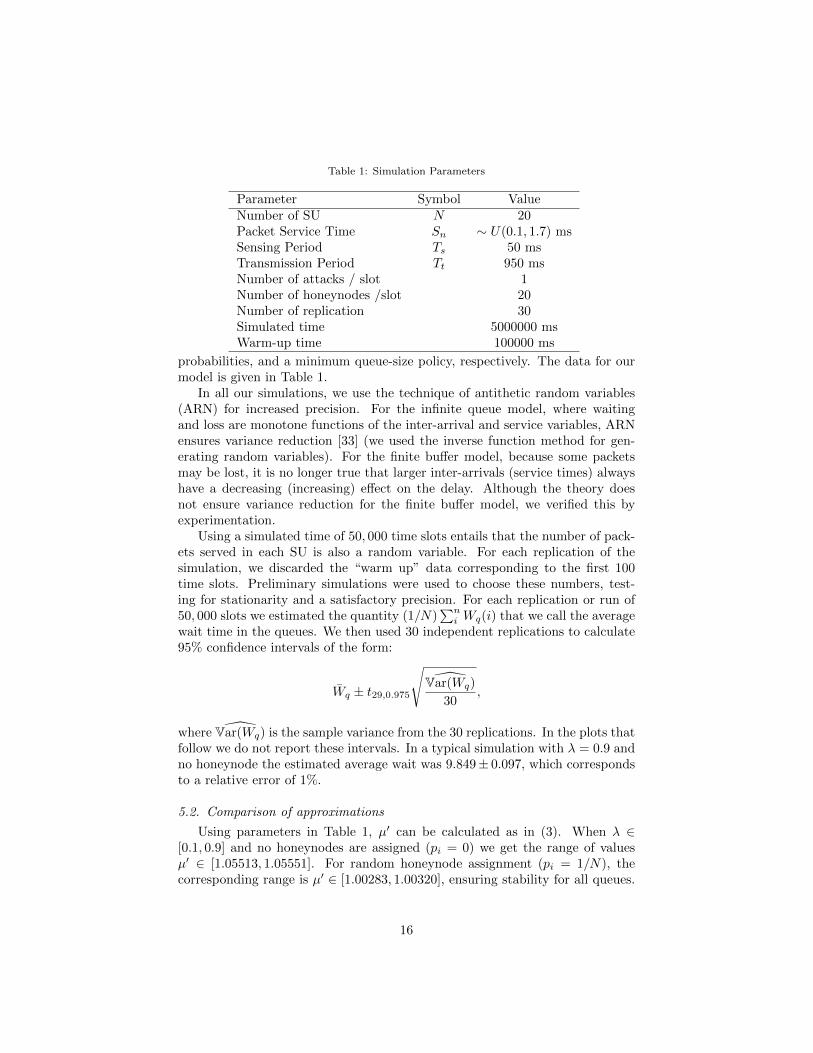
Table 1: Simulation Parameters

Parameter Symbol ValueNumber of SU N 20Packet Service Time Sn ∼ U(0.1, 1.7) msSensing Period Ts 50 msTransmission Period Tt 950 msNumber of attacks / slot 1Number of honeynodes /slot 20Number of replication 30Simulated time 5000000 msWarm-up time 100000 ms

probabilities, and a minimum queue-size policy, respectively. The data for ourmodel is given in Table 1.

In all our simulations, we use the technique of antithetic random variables(ARN) for increased precision. For the infinite queue model, where waitingand loss are monotone functions of the inter-arrival and service variables, ARNensures variance reduction [33] (we used the inverse function method for gen-erating random variables). For the finite buffer model, because some packetsmay be lost, it is no longer true that larger inter-arrivals (service times) alwayshave a decreasing (increasing) effect on the delay. Although the theory doesnot ensure variance reduction for the finite buffer model, we verified this byexperimentation.

Using a simulated time of 50, 000 time slots entails that the number of pack-ets served in each SU is also a random variable. For each replication of thesimulation, we discarded the “warm up” data corresponding to the first 100time slots. Preliminary simulations were used to choose these numbers, test-ing for stationarity and a satisfactory precision. For each replication or run of50, 000 slots we estimated the quantity (1/N)

∑ni Wq(i) that we call the average

wait time in the queues. We then used 30 independent replications to calculate95% confidence intervals of the form:

Wq ± t29,0.975

√Var(Wq)

30,

where Var(Wq) is the sample variance from the 30 replications. In the plots thatfollow we do not report these intervals. In a typical simulation with λ = 0.9 andno honeynode the estimated average wait was 9.849± 0.097, which correspondsto a relative error of 1%.

5.2. Comparison of approximations

Using parameters in Table 1, µ′ can be calculated as in (3). When λ ∈[0.1, 0.9] and no honeynodes are assigned (pi = 0) we get the range of valuesµ′ ∈ [1.05513, 1.05551]. For random honeynode assignment (pi = 1/N), thecorresponding range is µ′ ∈ [1.00283, 1.00320], ensuring stability for all queues.

16

0

2

4

6

8

10

12

14

0.1 0.2 0.3 0.4 0.5 0.6 0.7 0.8 0.9

Avera

ge Q

ueuin

g D

ela

y in m

illis

econd

Packet Arrival Rate (λ)

M/G/1 ApproximationPriority Queue

Queue with VacationSimulated

(a) without Honeynode

0

50

100

150

200

250

300

0.1 0.2 0.3 0.4 0.5 0.6 0.7 0.8 0.9

Avera

ge Q

ueuin

g D

ela

y in m

illis

econd

Packet Arrival Rate (λ)

Priority QueueSimulated

M/G/1 ApproximationQueue with Vacation

(b) With one HoneynodeFigure 6: Average Queuing Delay for simple cognitive radio network

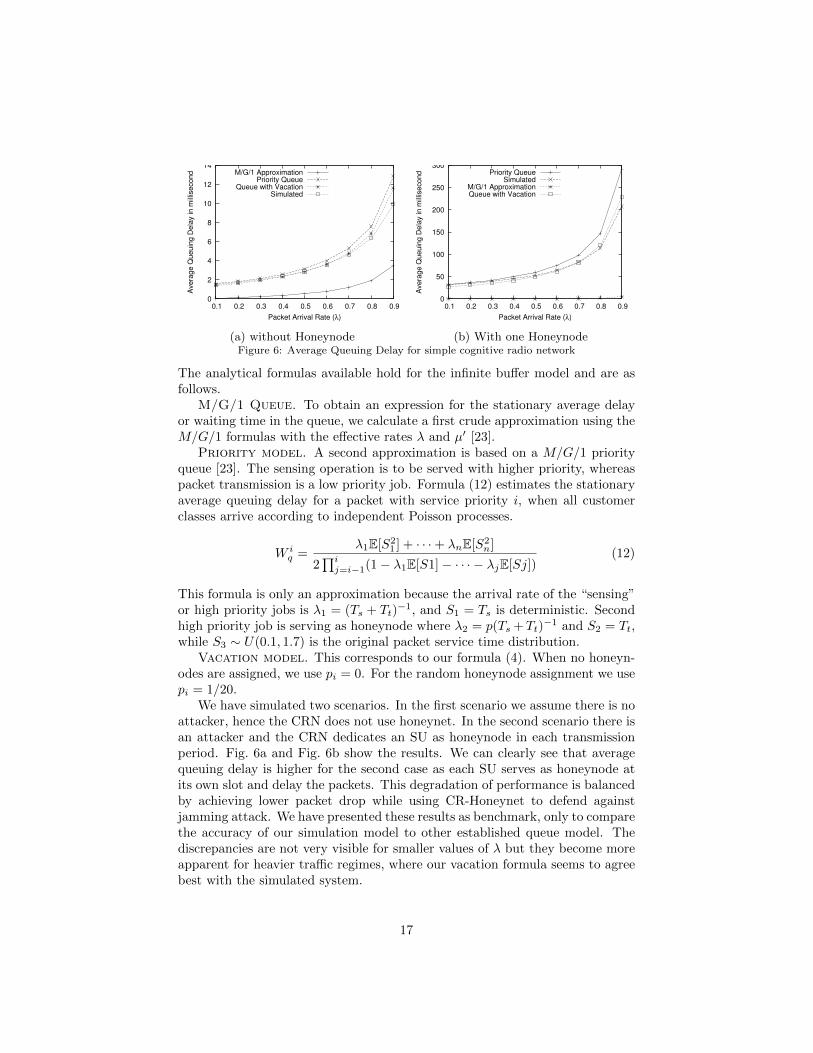
The analytical formulas available hold for the infinite buffer model and are asfollows.

M/G/1 Queue. To obtain an expression for the stationary average delayor waiting time in the queue, we calculate a first crude approximation using theM/G/1 formulas with the effective rates λ and µ′ [23].

Priority model. A second approximation is based on a M/G/1 priorityqueue [23]. The sensing operation is to be served with higher priority, whereaspacket transmission is a low priority job. Formula (12) estimates the stationaryaverage queuing delay for a packet with service priority i, when all customerclasses arrive according to independent Poisson processes.

W iq =

λ1E[S21 ] + · · ·+ λnE[S2

n]

2∏ij=i−1(1− λ1E[S1]− · · · − λjE[Sj])

(12)

This formula is only an approximation because the arrival rate of the “sensing”or high priority jobs is λ1 = (Ts + Tt)

−1, and S1 = Ts is deterministic. Secondhigh priority job is serving as honeynode where λ2 = p(Ts +Tt)

−1 and S2 = Tt,while S3 ∼ U(0.1, 1.7) is the original packet service time distribution.

Vacation model. This corresponds to our formula (4). When no honeyn-odes are assigned, we use pi = 0. For the random honeynode assignment we usepi = 1/20.

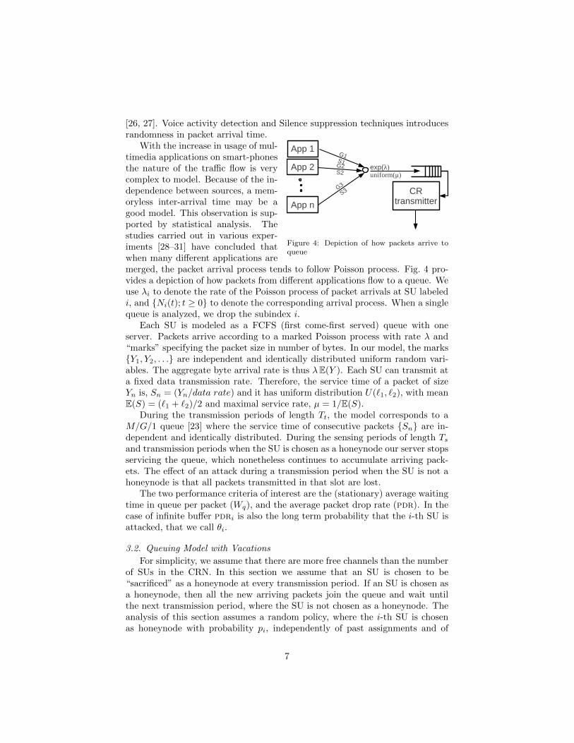
We have simulated two scenarios. In the first scenario we assume there is noattacker, hence the CRN does not use honeynet. In the second scenario there isan attacker and the CRN dedicates an SU as honeynode in each transmissionperiod. Fig. 6a and Fig. 6b show the results. We can clearly see that averagequeuing delay is higher for the second case as each SU serves as honeynode atits own slot and delay the packets. This degradation of performance is balancedby achieving lower packet drop while using CR-Honeynet to defend againstjamming attack. We have presented these results as benchmark, only to comparethe accuracy of our simulation model to other established queue model. Thediscrepancies are not very visible for smaller values of λ but they become moreapparent for heavier traffic regimes, where our vacation formula seems to agreebest with the simulated system.

17

0.1 0.2 0.3 0.4 0.5 0.6 0.7 0.8 0.9Packet arrival rate (λ)

0

50

100

150

200

250

300Av

erag

e qu

euin

g de

lay

in m

swithout honeynetRound RobinMinimum queueRandom honeynode

(a) Average Queuing Delay in millisecondfor ξ = 0.8

0.1 0.2 0.3 0.4 0.5 0.6 0.7 0.8 0.9 1.0Attractiveness of Honeynet (ξ)

0.00

0.01

0.02

0.03

0.04

0.05

0.06

Averag

e PD

R

without honeynetRound RobinMinimum queueRandom honeynode

(b) Average pdr of all SUs for λ = 0.6

Figure 7: Results for CRN with infinite buffer

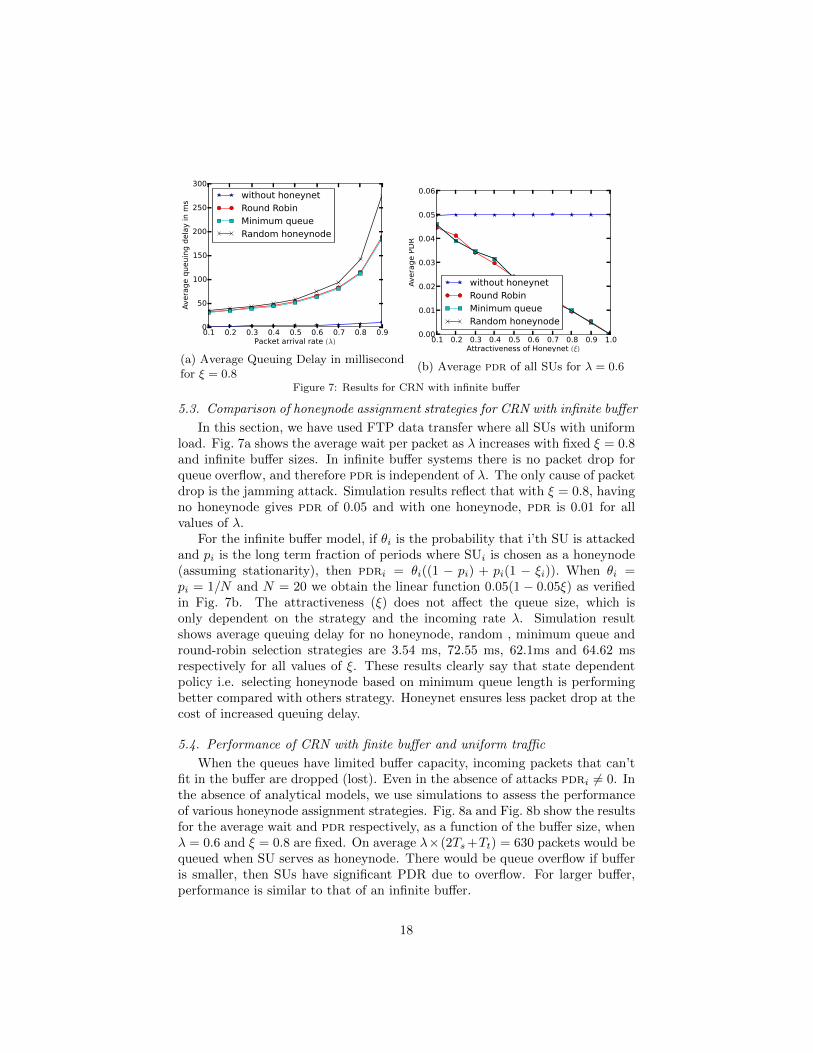
5.3. Comparison of honeynode assignment strategies for CRN with infinite buffer

In this section, we have used FTP data transfer where all SUs with uniformload. Fig. 7a shows the average wait per packet as λ increases with fixed ξ = 0.8and infinite buffer sizes. In infinite buffer systems there is no packet drop forqueue overflow, and therefore pdr is independent of λ. The only cause of packetdrop is the jamming attack. Simulation results reflect that with ξ = 0.8, havingno honeynode gives pdr of 0.05 and with one honeynode, pdr is 0.01 for allvalues of λ.

For the infinite buffer model, if θi is the probability that i’th SU is attackedand pi is the long term fraction of periods where SUi is chosen as a honeynode(assuming stationarity), then pdri = θi((1 − pi) + pi(1 − ξi)). When θi =pi = 1/N and N = 20 we obtain the linear function 0.05(1 − 0.05ξ) as verifiedin Fig. 7b. The attractiveness (ξ) does not affect the queue size, which isonly dependent on the strategy and the incoming rate λ. Simulation resultshows average queuing delay for no honeynode, random , minimum queue andround-robin selection strategies are 3.54 ms, 72.55 ms, 62.1ms and 64.62 msrespectively for all values of ξ. These results clearly say that state dependentpolicy i.e. selecting honeynode based on minimum queue length is performingbetter compared with others strategy. Honeynet ensures less packet drop at thecost of increased queuing delay.

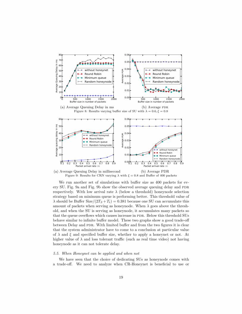
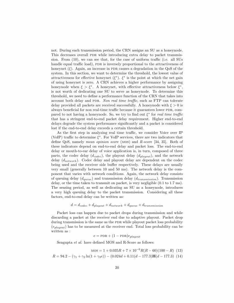
5.4. Performance of CRN with finite buffer and uniform traffic

When the queues have limited buffer capacity, incoming packets that can’tfit in the buffer are dropped (lost). Even in the absence of attacks pdri 6= 0. Inthe absence of analytical models, we use simulations to assess the performanceof various honeynode assignment strategies. Fig. 8a and Fig. 8b show the resultsfor the average wait and pdr respectively, as a function of the buffer size, whenλ = 0.6 and ξ = 0.8 are fixed. On average λ×(2Ts+Tt) = 630 packets would bequeued when SU serves as honeynode. There would be queue overflow if bufferis smaller, then SUs have significant PDR due to overflow. For larger buffer,performance is similar to that of an infinite buffer.

18

0 500 1000 1500 2000Buffer size in number of packets

0

10

20

30

40

50

60

70

80Av

erag

e Qu

euin

g De

lay

in m

s

without honeynetRound RobinMinimum queueRandom honeynode

(a) Average Queuing Delay in ms

0 500 1000 1500 2000Buffer size in number of packets

0.00

0.01

0.02

0.03

0.04

0.05

0.06

Aver

age

PDR without honeynet

Round RobinMinimum queueRandom honeynode

(b) Average pdrFigure 8: Results varying buffer size of SU with λ = 0.6, ξ = 0.8

0.1 0.2 0.3 0.4 0.5 0.6 0.7 0.8 0.9Packet arrival rate (λ)

0

10

20

30

40

50

60

Aver

age

queu

ing

dela

y in

ms

without honeynetRound RobinMinimum queueRandom honeynode

(a) Average Queuing Delay in millisecond

0.1 0.2 0.3 0.4 0.5 0.6 0.7 0.8 0.9Packet arrival rate (λ)

0.00

0.01

0.02

0.03

0.04

0.05

0.06Av

erag

e PD

R

without honeynetRound RobinMinimum queueRandom honeynode

(b) Average PDRFigure 9: Results for CRN varying λ with ξ = 0.8 and Buffer of 400 packets

We run another set of simulations with buffer size as 400 packets for ev-ery SU. Fig. 9a and Fig. 9b show the observed average queuing delay and pdrrespectively. With low arrival rate λ (below a threshold) honeynode selectionstrategy based on minimum queue is performing better. This threshold value ofλ should be Buffer Size/(2TS +Tt) = 0.381 because one SU can accumulate thisamount of packets when serving as honeynode. When λ goes above the thresh-old, and when the SU is serving as honeynode, it accumulates many packets sothat the queue overflows which causes increase in pdr. Below this threshold SUsbehave similar to infinite buffer model. These two graphs show a good trade-offbetween Delay and pdr. With limited buffer and from the two figures it is clearthat the system administrator have to come to a conclusion at particular valueof λ and ξ and specified buffer size, whether to apply a honeynet or not. Athigher value of λ and loss tolerant traffic (such as real time video) not havinghoneynode as it can not tolerate delay.

5.5. When Honeynet can be applied and when not

We have seen that the choice of dedicating SUs as honeynode comes witha trade-off. We need to analyze when CR-Honeynet is beneficial to use or

19

not. During each transmission period, the CRN assigns an SU as a honeynode.This decreases overall pdr while introducing extra delay to packet transmis-sion. From (10), we can see that, for the case of uniform traffic (i.e. all SUshandle equal traffic load), pdr is inversely proportional to the attractiveness ofhoneynet (ξ). Again, an increase in pdr causes a degradation in the QoS of thesystem. In this section, we want to determine the threshold, the lowest value ofattractiveness for effective honeynet (ξ∗). ξ∗ is the point at which the net gainof using honeynet is zero. A CRN achieves a higher performance by assigninghoneynode when ξ > ξ∗. A honeynet, with effective attractiveness below ξ∗,is not worth of dedicating one SU to serve as honeynode. To determine thisthreshold, we need to define a performance function of the CRN that takes intoaccount both delay and pdr. Non real time traffic, such as FTP can toleratedelay provided all packets are received successfully. A honeynode with ξ > 0 isalways beneficial for non real-time traffic because it guarantees lower pdr, com-pared to not having a honeynode. So, we try to find out ξ∗ for real time trafficthat has a stringent end-to-end packet delay requirement. Higher end-to-enddelays degrade the system performance significantly and a packet is consideredlost if the end-to-end delay exceeds a certain threshold.

As the first step in analyzing real time traffic, we consider Voice over IP(VoIP) traffic to determine ξ∗. For VoIP services, there are two indicators thatdefine QoS, namely mean opinion score (mos) and R-score [34, 35]. Both ofthese indicators depend on end-to-end delay and packet loss. The end-to-enddelay or mouth-to-ear delay of voice application is, in turn, composed of threeparts, the codec delay (dcodec), the playout delay (dplayout), and the networkdelay (dnetwork). Codec delay and playout delay are dependent on the codecbeing used and the receiver side buffer respectively. These delays are usuallyvery small (generally between 10 and 50 ms). The network delay is the com-ponent that varies with network conditions. Again, the network delay consistsof queuing delay (dqueue) and transmission delay (dtransmission). Transmissiondelay, or the time taken to transmit on packet, is very negligible (0.1 to 1.7 ms).The sensing period, as well as dedicating an SU as a honeynode, introducesa very high queuing delay to the packet transmission. Considering all thesefactors, end-to-end delay can be written as:

d = dcodec + dplayout + dnetwork + dqueue + dtransmission

Packet loss can happen due to packet drops during transmission and whilediscarding a packet at the receiver end due to adaptive playout. Packet dropduring transmission is the same as the pdr while playout packet loss probability(eplayout) has to be measured at the receiver end. Total loss probability can bewritten as :

e = pdr + (1− pdr)eplayout

Sengupta et al. have defined MOS and R-Score as follows:

mos = 1 + 0.035R+ 7× 10−6R(R− 60)(100−R) (13)

R = 94.2− (γ1 + γ2 ln(1 + γ3e))− (0.024d+ 0.11(d− 177.3)H(d− 177.3) (14)

20

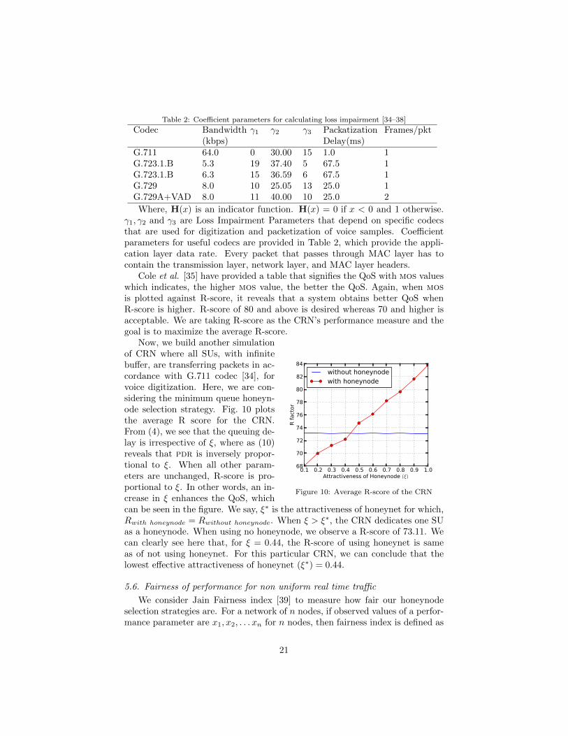
Table 2: Coefficient parameters for calculating loss impairment [34–38]

Codec Bandwidth(kbps)

γ1 γ2 γ3 PackatizationDelay(ms)

Frames/pkt

G.711 64.0 0 30.00 15 1.0 1G.723.1.B 5.3 19 37.40 5 67.5 1G.723.1.B 6.3 15 36.59 6 67.5 1G.729 8.0 10 25.05 13 25.0 1G.729A+VAD 8.0 11 40.00 10 25.0 2

Where, H(x) is an indicator function. H(x) = 0 if x < 0 and 1 otherwise.γ1, γ2 and γ3 are Loss Impairment Parameters that depend on specific codecsthat are used for digitization and packetization of voice samples. Coefficientparameters for useful codecs are provided in Table 2, which provide the appli-cation layer data rate. Every packet that passes through MAC layer has tocontain the transmission layer, network layer, and MAC layer headers.

Cole et al. [35] have provided a table that signifies the QoS with mos valueswhich indicates, the higher mos value, the better the QoS. Again, when mosis plotted against R-score, it reveals that a system obtains better QoS whenR-score is higher. R-score of 80 and above is desired whereas 70 and higher isacceptable. We are taking R-score as the CRN’s performance measure and thegoal is to maximize the average R-score.

0.1 0.2 0.3 0.4 0.5 0.6 0.7 0.8 0.9 1.0Attractiveness of Honeynode (ξ)

68

70

72

74

76

78

80

82

84

R factor

without honeynodewith honeynode

Figure 10: Average R-score of the CRN

Now, we build another simulationof CRN where all SUs, with infinitebuffer, are transferring packets in ac-cordance with G.711 codec [34], forvoice digitization. Here, we are con-sidering the minimum queue honeyn-ode selection strategy. Fig. 10 plotsthe average R score for the CRN.From (4), we see that the queuing de-lay is irrespective of ξ, where as (10)reveals that pdr is inversely propor-tional to ξ. When all other param-eters are unchanged, R-score is pro-portional to ξ. In other words, an in-crease in ξ enhances the QoS, whichcan be seen in the figure. We say, ξ∗ is the attractiveness of honeynet for which,Rwith honeynode = Rwithout honeynode. When ξ > ξ∗, the CRN dedicates one SUas a honeynode. When using no honeynode, we observe a R-score of 73.11. Wecan clearly see here that, for ξ = 0.44, the R-score of using honeynet is sameas of not using honeynet. For this particular CRN, we can conclude that thelowest effective attractiveness of honeynet (ξ∗) = 0.44.

5.6. Fairness of performance for non uniform real time traffic

We consider Jain Fairness index [39] to measure how fair our honeynodeselection strategies are. For a network of n nodes, if observed values of a perfor-mance parameter are x1, x2, . . . xn for n nodes, then fairness index is defined as

21

0.1-0.2 0.1-0.3 0.6-0.8 0.1-0.8Range of packet arrival rate λ

25

30

35

40

Averag

e Que

uing

Delay

RandomRound RobinMinimum Queue

(a) Average queuing delay

0.1-0.2 0.1-0.3 0.6-0.8 0.1-0.8Range of packet arrival rate λ

0.0

0.2

0.4

0.6

0.8

1.0

Fairn

ess

Inde

x of

que

uing

del

ay

RandomRound RobinMinimum Queue

(b) Fairness Index among all SUsFigure 11: Simulation results for CRN with non uniform traffic.

(∑n

i=1 xi)2

n∑n

i=1 x2i

. Fig. 11a and Fig. 11b depicts the overall average queuing delay for

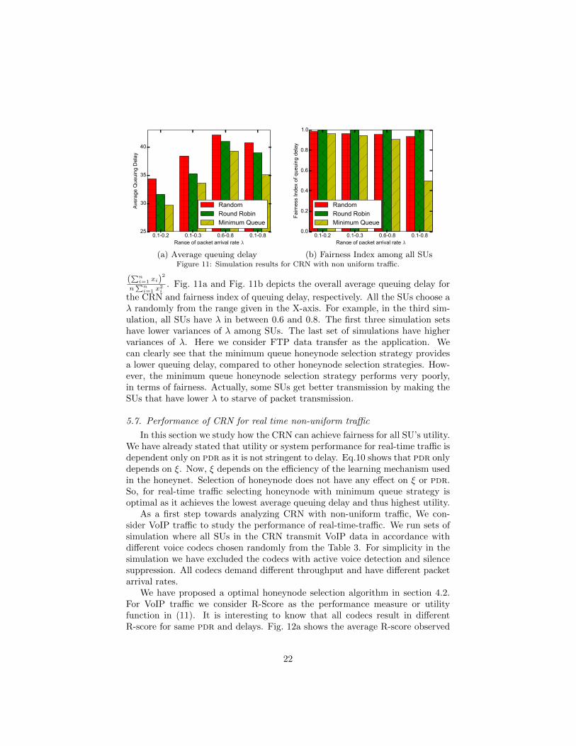
the CRN and fairness index of queuing delay, respectively. All the SUs choose aλ randomly from the range given in the X-axis. For example, in the third sim-ulation, all SUs have λ in between 0.6 and 0.8. The first three simulation setshave lower variances of λ among SUs. The last set of simulations have highervariances of λ. Here we consider FTP data transfer as the application. Wecan clearly see that the minimum queue honeynode selection strategy providesa lower queuing delay, compared to other honeynode selection strategies. How-ever, the minimum queue honeynode selection strategy performs very poorly,in terms of fairness. Actually, some SUs get better transmission by making theSUs that have lower λ to starve of packet transmission.

5.7. Performance of CRN for real time non-uniform traffic

In this section we study how the CRN can achieve fairness for all SU’s utility.We have already stated that utility or system performance for real-time traffic isdependent only on pdr as it is not stringent to delay. Eq.10 shows that pdr onlydepends on ξ. Now, ξ depends on the efficiency of the learning mechanism usedin the honeynet. Selection of honeynode does not have any effect on ξ or pdr.So, for real-time traffic selecting honeynode with minimum queue strategy isoptimal as it achieves the lowest average queuing delay and thus highest utility.

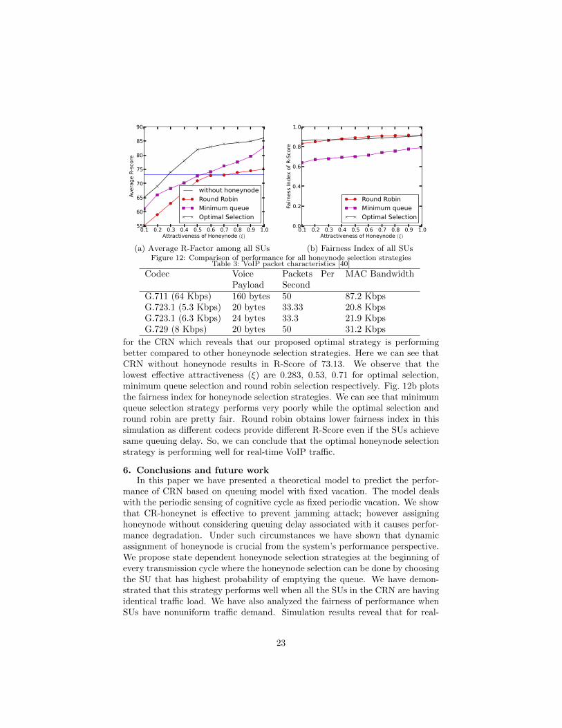
As a first step towards analyzing CRN with non-uniform traffic, We con-sider VoIP traffic to study the performance of real-time-traffic. We run sets ofsimulation where all SUs in the CRN transmit VoIP data in accordance withdifferent voice codecs chosen randomly from the Table 3. For simplicity in thesimulation we have excluded the codecs with active voice detection and silencesuppression. All codecs demand different throughput and have different packetarrival rates.

We have proposed a optimal honeynode selection algorithm in section 4.2.For VoIP traffic we consider R-Score as the performance measure or utilityfunction in (11). It is interesting to know that all codecs result in differentR-score for same pdr and delays. Fig. 12a shows the average R-score observed

22

0.1 0.2 0.3 0.4 0.5 0.6 0.7 0.8 0.9 1.0Attractiveness of Honeynode (ξ)

55

60

65

70

75

80

85

90Average R-score

without honeynodeRound RobinMinimum queueOptimal Selection

(a) Average R-Factor among all SUs

0.1 0.2 0.3 0.4 0.5 0.6 0.7 0.8 0.9 1.0Attractiveness of Honeynode (ξ)

0.0

0.2

0.4

0.6

0.8

1.0

Fairn

ess Index of R-Score

Round RobinMinimum queueOptimal Selection

(b) Fairness Index of all SUsFigure 12: Comparison of performance for all honeynode selection strategies

Table 3: VoIP packet characteristics [40]

Codec VoicePayload

Packets PerSecond

MAC Bandwidth

G.711 (64 Kbps) 160 bytes 50 87.2 KbpsG.723.1 (5.3 Kbps) 20 bytes 33.33 20.8 KbpsG.723.1 (6.3 Kbps) 24 bytes 33.3 21.9 KbpsG.729 (8 Kbps) 20 bytes 50 31.2 Kbps

for the CRN which reveals that our proposed optimal strategy is performingbetter compared to other honeynode selection strategies. Here we can see thatCRN without honeynode results in R-Score of 73.13. We observe that thelowest effective attractiveness (ξ) are 0.283, 0.53, 0.71 for optimal selection,minimum queue selection and round robin selection respectively. Fig. 12b plotsthe fairness index for honeynode selection strategies. We can see that minimumqueue selection strategy performs very poorly while the optimal selection andround robin are pretty fair. Round robin obtains lower fairness index in thissimulation as different codecs provide different R-Score even if the SUs achievesame queuing delay. So, we can conclude that the optimal honeynode selectionstrategy is performing well for real-time VoIP traffic.

6. Conclusions and future workIn this paper we have presented a theoretical model to predict the perfor-

mance of CRN based on queuing model with fixed vacation. The model dealswith the periodic sensing of cognitive cycle as fixed periodic vacation. We showthat CR-honeynet is effective to prevent jamming attack; however assigninghoneynode without considering queuing delay associated with it causes perfor-mance degradation. Under such circumstances we have shown that dynamicassignment of honeynode is crucial from the system’s performance perspective.We propose state dependent honeynode selection strategies at the beginning ofevery transmission cycle where the honeynode selection can be done by choosingthe SU that has highest probability of emptying the queue. We have demon-strated that this strategy performs well when all the SUs in the CRN are havingidentical traffic load. We have also analyzed the fairness of performance whenSUs have nonuniform traffic demand. Simulation results reveal that for real-

23

time traffic our proposed honeynode selection strategy provides optimal systemperformance while maintaining fairness.

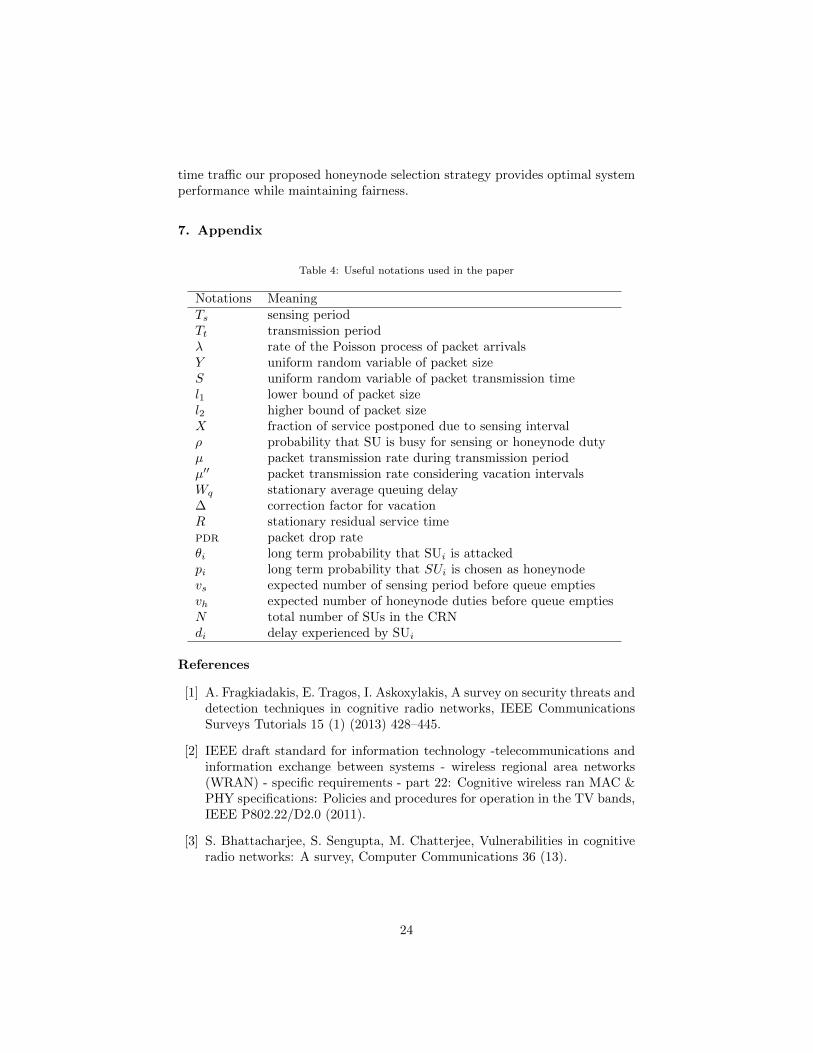
7. Appendix

Table 4: Useful notations used in the paper

Notations MeaningTs sensing periodTt transmission periodλ rate of the Poisson process of packet arrivalsY uniform random variable of packet sizeS uniform random variable of packet transmission timel1 lower bound of packet sizel2 higher bound of packet sizeX fraction of service postponed due to sensing intervalρ probability that SU is busy for sensing or honeynode dutyµ packet transmission rate during transmission periodµ′′ packet transmission rate considering vacation intervalsWq stationary average queuing delay∆ correction factor for vacationR stationary residual service timepdr packet drop rateθi long term probability that SUi is attackedpi long term probability that SUi is chosen as honeynodevs expected number of sensing period before queue emptiesvh expected number of honeynode duties before queue emptiesN total number of SUs in the CRNdi delay experienced by SUi

References

[1] A. Fragkiadakis, E. Tragos, I. Askoxylakis, A survey on security threats anddetection techniques in cognitive radio networks, IEEE CommunicationsSurveys Tutorials 15 (1) (2013) 428–445.

[2] IEEE draft standard for information technology -telecommunications andinformation exchange between systems - wireless regional area networks(WRAN) - specific requirements - part 22: Cognitive wireless ran MAC &PHY specifications: Policies and procedures for operation in the TV bands,IEEE P802.22/D2.0 (2011).

[3] S. Bhattacharjee, S. Sengupta, M. Chatterjee, Vulnerabilities in cognitiveradio networks: A survey, Computer Communications 36 (13).

24

[4] T. X. Brown, J. E. James, A. Sethi, Jamming and sensing of encryptedwireless ad hoc networks, in: Proceedings of the ACM international sym-posium on Mobile ad hoc networking and computing, 2006, pp. 120–130.

[5] W. Xu, T. Wood, W. Trappe, Y. Zhang, Channel surfing and spatial re-treats: defenses against wireless denial of service, in: Proceedings of the3rd ACM workshop on Wireless security, ACM, 2004, pp. 80–89.

[6] V. Navda, A. Bohra, S. Ganguly, D. Rubenstein, Using channel hopping toincrease 802.11 resilience to jamming attacks, in: 26th IEEE InternationalConference on Computer Communications (INFOCOM), IEEE, 2007.

[7] W. Xu, K. Ma, W. Trappe, Y. Zhang, Jamming sensor networks: attackand defense strategies, Network, IEEE (2006) 41–47.

[8] C. Sorrells, P. Potier, L. Qian, X. Li, Anomalous spectrum usage attackdetection in cognitive radio wireless networks, in: IEEE International Con-ference on Technologies for Homeland Security (HST), 2011, IEEE, 2011,pp. 384–389.

[9] C. Popper, M. Strasser, S. Capkun, Anti-jamming broadcast communica-tion using uncoordinated spread spectrum techniques, Selected Areas inCommunications, IEEE Journal on 28 (5) (2010) 703–715.

[10] S. Misra, S. K. Dhurandher, A. Rayankula, D. Agrawal, Using honeyn-odes for defense against jamming attacks in wireless infrastructure-basednetworks, Computers and Electrical Engineering 36 (2) (2010) 367 – 382.

[11] S. Bhunia, S. Sengupta, F. Vazquez-Abad, Cr-honeynet: A learning &decoy based sustenance mechanism against jamming attack in crn, in: Mil-itary Communications Conference (MILCOM), 2014 IEEE, IEEE, 2014,pp. 1173–1180.

[12] J. Burbank, Security in cognitive radio networks: The required evolution inapproaches to wireless network security, in: 3rd International Conference onCognitive Radio Oriented Wireless Networks and Communications., 2008,pp. 1 –7. doi:10.1109/CROWNCOM.2008.4562536.

[13] Wi-spy spectrum analyzer, http://www.metageek.net/products/wi-spy/.

[14] GNU Radio, http://gnuradio.org/redmine/projects/gnuradio/wiki.

[15] Usrp kit, https://www.ettus.com/product/details/UN200-KIT.

[16] K. Pelechrinis, M. Iliofotou, S. V. Krishnamurthy, Denial of service attacksin wireless networks: The case of jammers, Communications Surveys &Tutorials, IEEE 13 (2) (2011) 245–257.

25

[17] V. Chatzigiannakis, G. Androulidakis, K. Pelechrinis, S. Papavassiliou,V. Maglaris, Data fusion algorithms for network anomaly detection: clas-sification and evaluation, in: Networking and Services, 2007. ICNS. ThirdInternational Conference on, IEEE, 2007, pp. 50–50.

[18] C. Sorrells, L. Qian, H. Li, Quickest detection of denial-of-service attacksin cognitive wireless networks, in: Homeland Security (HST), 2012 IEEEConference on Technologies for, IEEE, 2012, pp. 580–584.

[19] T. X. Brown, A. Sethi, Potential cognitive radio denial-of-service vulnera-bilities and protection countermeasures: A multi-dimensional analysis andassessment, Mobile Networks and Applications 13 (5) (2008) 516–532.

[20] S. Anand, S. Sengupta, K. Hong, K. Subbalakshmi, R. Chandramouli,H. Cam, Exploiting channel fragmentation and aggregation/ bonding tocreate security vulnerabilities, IEEE Transactions on Vehicular Technology.

[21] B. Wang, Y. Wu, K. R. Liu, T. C. Clancy, An anti-jamming stochas-tic game for cognitive radio networks, Selected Areas in Communications,IEEE Journal on 29 (4) (2011) 877–889.

[22] K. C. Madan, A. Z. Abu Al-Rub, On a single server queue with optionalphase type server vacations based on exhaustive deterministic service anda single vacation policy, Applied Mathematics and Computation 149 (3)(2004) 723–734.

[23] S. M. Ross, Introduction to Probability Models, 10thEd., Academic Press.

[24] G. Choudhury, L. Tadj, An M/G/1 queue with two phases of service sub-ject to the server breakdown and delayed repair, Applied MathematicalModelling 33 (6) (2009) 2699–2709.

[25] S. Wang, J. Zhang, L. Tong, Delay analysis for cognitive radio networkswith random access: a fluid queue view, in: INFOCOM, 2010 ProceedingsIEEE, IEEE, 2010, pp. 1–9.

[26] L. X. Cai, X. Shen, J. W. Mark, L. Cai, Y. Xiao, Voice capacity analysisof wlan with unbalanced traffic, Vehicular Technology, IEEE Transactionson 55 (3) (2006) 752–761.

[27] L. Sun, E. Ifeachor, Voice quality prediction models and their applicationin voip networks, IEEE Transactions on Multimedia 8 (4) (2006) 809 –820.doi:10.1109/TMM.2006.876279.

[28] V. Grout, S. Cunningham, D. Oram, R. Hebblewhite, A note on the distri-bution of packet arrivals in high-speed data networks., in: ICWI, Citeseer,2004, pp. 889–892.

[29] R. Jain, S. A. Routhier, Packet trains-measurements and a new model forcomputer network traffic, IEEE Journal on Selected Areas in Communica-tion 6 (4) (1986) 986–995.

26

[30] M. Wilson, A historical view of network traffic models,http://www.cse.wustl.edu /∼ jain/cse567-06/ftp/traffic models2.

[31] D. R. Dennis Guster, R. Sundheim, Evaluating computer networkpacket inter-arrival distributions, Encyclopedia of Information Science &Technologydoi:10.4018/978-1-60566-026-4.ch232.

[32] R. Kaas, M. Goovaerts, J. Dhaene, M. Denuit, Modern actuarial risk theory,Vol. 328, Springer, 2001.

[33] S. M. Ross, Simulation, 5th Edision, Academic Press, 2012.

[34] S. Sengupta, M. Chatterjee, S. Ganguly, Improving quality of voip streamsover wimax, Computers, IEEE Transactions on 57 (2) (2008) 145–156.

[35] R. G. Cole, J. H. Rosenbluth, Voice over IP performance monitoring, ACMSIGCOMM Computer Communication Review 31 (2) (2001) 9–24.

[36] L. Ding, R. A. Goubran, Speech quality prediction in voip using theextended e-model, in: Global Telecommunications Conference, 2003.GLOBECOM’03. IEEE, Vol. 7, IEEE, 2003, pp. 3974–3978.

[37] J. Q. Walker, Assessing voip call quality using the e-model.URL http://www.recursosvoip.com/docs/english/AssessingVoIPCallQualityUsingtheE-model.pdf

[38] V. Balan, L. Eggert, An experimental evaluation of voice-over-ip qualityover the datagram congestion control protocol, School of Engineering andScienze International University Bremen.

[39] R. Jain, D.-M. Chiu, W. R. Hawe, A quantitative measure of fairness anddiscrimination for resource allocation in shared computer system, EasternResearch Laboratory, Digital Equipment Corporation, 1984.

[40] Voice Over IP - per call bandwidth consumption.URL http://www.cisco.com/c/en/us/support/docs/voice/voice-quality/7934-bwidth-consume.html

27