Embed Size (px)
Citation preview
PERFORMANCE, DENITRIFICATION ACTIVITY, AND MICROBIAL COMMUNITY
DYNAMICS OF DENITRIFYING BIOFILTERS UNDER FLUCTUATING WATER LEVEL
BY
SARAH KINGSLEY HATHAWAY
THESIS
Submitted in partial fulfillment of the requirements
for the degree of Master of Science in Environmental Engineering in Civil Engineering
in the Graduate College of the
University of Illinois at Urbana-Champaign, 2013
Urbana, Illinois
Advisers:
Research Assistant Professor Julie L. Zilles
Associate Professor Angela D. Kent
ii
Abstract
Agricultural runoff through tile drainage systems is a significant source of nitrogen to
coastal water bodies, causing water quality degradation. Denitrifying biofilters have been
identified as a technology that reduces the export of nitrate from tile-drained fields. A better
understanding of the microbial communities that allow the biofilter to function may provide
insight to improve performance.
Two studies were performed to achieve this aim. Laboratory-scale biofilters were
operated for two years with variations in water level. Nitrate removal performance was
measured. Denitrifying enzyme assays (DEAs) were performed regularly to measure the
denitrification potential in different parts of the two reactors. A comparison of the microbial
communities of agriculture, natural wetland, restored wetland, and biofilter habitats was also
carried out to determine the relative effects of niche and legacy on the structure of the microbial
communities. For both studies, total bacterial communities were analyzed using automated
ribosomal intergenic spacer analysis (ARISA), and denitrifying bacterial communities were
analyzed using terminal restriction fragment length polymorphism (tRFLP) of nosZ, the gene
encoding the catalytic subunit of nitrous oxide reduction.
In the laboratory biofilter study, the performance was sensitive to changing water level,
with 31% nitrate removed at high water level and 59% at low water level. The denitrification
potential was the same under almost all conditions, ranging from 0.000015-0.004 mg N2O-
N/hour/dry g woodchip; the microbial communities were still able to carry out denitrification,
unaffected by the water level, unless dried out for an extended period of time. The denitrifying
bacterial communities were not significantly different from each other, regardless of water level.
This indicates resistance of these bacteria, meaning that the bacterial communities did not change
iii
in response to disturbance. The total bacterial communities became more distinct between the
two reactors once the regular disturbance period began, with a stronger effect on the most
severely disturbed port. The communities were not distinguishable based on high or low water
level, though, in the same place during the regular disturbance period, indicating that disturbance
communities were created, rather than high or low water level communities.
In the habitat comparison, the biofilter microbial communities were distinct from those of
the other habitats. This was true for both the total and denitrifying bacterial communities. This
suggests a stronger influence of environmental parameters on the microbial community structure
than the legacy effects of the agricultural bacteria that were initially present and continued to
enter with the influent water.
These results show the biofilters to be stable systems with resistant and functionally
redundant bacterial communities. Water level and HRT should be considered in the design of
the biofilters, as they influenced the nitrate removal. Overall, the biofilters show promise as a
method to reduce the amount of nitrogen pollution from agricultural fields to surface water.

iv
Acknowledgements I would like to thank my advisors, Dr. Julie Zilles and Dr. Angela Kent. I would like to
express my gratitude to Dr. Zilles for her excellent feedback on my writing and managing my
time and for challenging me to think carefully about the questions I’m asking and how best to
answer them. I am appreciative of Dr. Kent for introducing me to microbial ecology and the lab
techniques and multivariate statistics that go with it, as well as for her never-ending enthusiasm.
Thanks must also go to the rest of the biofilter group: Dr. Luis Rodríguez, for his
helpfulness and feedback in biofilter meetings. Graham Kent helped me in the field. I am
grateful to Dora Boyd Cohen for good discussions about our work and also, for her friendship.
Paul Choi put in frequent hard work to help me in lab. Nick Bartolerio helped me get on my feet
in lab with the biofilters, and he and Matt Porter were always helpful and willing to share
information with me after leaving Urbana-Champaign.
The members of the Kent and Zilles labs have been wonderful colleagues, and, in
particular, Sara Paver and Jason Koval helped me as I learned new lab techniques. Corey
Mitchell has also been wonderfully helpful when I was using the GC.
I would also like to express my gratitude to my wonderful friends and family for all their
support. Thanks especially to Adrian, for his patience, encouragement, and willingness to bring
dinner during late nights in lab.
v
Table of Contents
Chapter 1: Introduction ................................................................................................................... 1
Chapter 2: Literature Review .......................................................................................................... 5
2.1 Denitrification ....................................................................................................................... 5
2.2 Denitrifying Biofilters ........................................................................................................... 9
2.3 Niche-Legacy Effects .......................................................................................................... 16
Chapter 3: Methods ....................................................................................................................... 24
3.1 Reactor Set-up ..................................................................................................................... 24
3.2 Reactor Operation ............................................................................................................... 25
3.3 Nitrate Concentrations......................................................................................................... 29
3.4 Microbial Community Sample Collection .......................................................................... 29
3.5 DNA Extraction................................................................................................................... 30
3.6 Microbial Community Analysis .......................................................................................... 31
3.7 Microbial Community Statistical Analysis ......................................................................... 33
3.8 Denitrification Potential ...................................................................................................... 33
3.9 Statistical Analysis of Denitrification Potential .................................................................. 34
3.10 Tracer Studies .................................................................................................................... 35
3.11 Dissolved Oxygen Measurements ..................................................................................... 36
3.12 Analytical Measurements .................................................................................................. 36
Chapter 4: Results of Laboratory Biofilter Study ......................................................................... 38
4.1 Reactor Performance ........................................................................................................... 38
4.2 Denitrification Potential ...................................................................................................... 39
4.3 Microbial Community Composition ................................................................................... 45
4.4 Tracer Studies ...................................................................................................................... 53
4.5 Dissolved Oxygen ............................................................................................................... 54
Chapter 5: Results of Niche-Legacy Effects Study ...................................................................... 55
5.1 Total Bacterial Communities .............................................................................................. 55
5.2 Denitrifying Bacterial Communities ................................................................................... 56
Chapter 6: Discussion ................................................................................................................... 58
6.1 Laboratory Biofilters ........................................................................................................... 58
vi
6.2 Niche-legacy Study ............................................................................................................. 65
Chapter 7: Conclusions ................................................................................................................. 67
References ..................................................................................................................................... 71
Appendix ....................................................................................................................................... 77
A.1 Laboratory Procedures ....................................................................................................... 77
A.2 Sample Information ............................................................................................................ 81
1
Chapter 1: Introduction
Human activity has caused radical alteration to the global nitrogen and phosphorus
cycles. In particular, the widespread use of synthetic fertilizer in modern farming has increased
nutrient loads to water bodies. The rate these nutrients are transported from land to ocean has
more than doubled compared to the non-anthropogenically influenced rate (Howarth et al, 2000).
Excess nutrient loading in water bodies is a major cause of water quality degradation.
Fertilization of surface water encourages the growth of excess algae. The eventual
decomposition of the algae depletes dissolved oxygen in the water, creating hypoxic zones. This
can lead to fish kills, which are particularly problematic in hypoxic areas with significant fishing
industries, like the Chesapeake Bay and Gulf of Mexico. Some of the algal blooms are made up
of toxic red tide organisms, which result in fish kills, and in some cases, human poisoning by
shellfish and death of marine mammals. Algal blooms also alter the environment by changing
the light patterns in the water. All these changes in the aquatic habitat favor different species
than are naturally present and can result in biodiversity losses.
Although the chemistry of different water bodies varies, a review of research on nutrient
limitation in coastal marine ecosystems suggests that many coastal ecosystems where hypoxia is
a problem are nitrogen-limited (Howarth & Marino, 2006). Thus, it is important for efforts to
reduce nutrient pollution to focus on preventing the release of excess nitrogen into coastal
ecosystems.
One of the sources of nitrogen in these ecosystems is agricultural runoff. Tile drain usage
is widespread in the agricultural Midwest, and subsurface runoff from fertilized agricultural
2
fields with tile drainage is a major source of nitrate in the Mississippi River Basin, which
discharges to the Gulf of Mexico (David et al, 2010). In central Illinois, twelve year average
nitrate losses from tile-drained agricultural fields were 23 to 33 kg N/ha, with average nitrate
concentrations from 15 to 20 mg N/L in subsurface drains (Kalita et al, 2006), higher than the
EPA maximum contaminant level for drinking water (10 mg/L).
Agricultural runoff poses treatment challenges, because it is a dispersed source of
pollution and cannot easily be diverted to a centralized treatment plant. Treatment technologies
must be sufficiently small-scale and low-maintenance to be employed next to cropped fields or
runoff-receiving bodies. Methods to decrease nitrogen export in runoff include biological
treatment systems like constructed wetlands (Carleton et al, 2001), decreased fertilizer use, and
slowing the flow of runoff with buffer strips (Osborne & Kovacic, 1993, Gopalakrishnan et al,
2012) or drainage ditches.
Another such option is edge-of-field denitrifying biofilters. These biofilters consist of a
trench of woodchips through which tile drainage is directed. The woodchips provide a filter
media on which bacteria can grow as well as a carbon source for denitrification. The biofilters
provide an environment in which denitrification can occur, reducing the nitrate load carried by
the tile drainage water to surface water. Denitrifying biofilters have been implemented with
success in Illinois (Wildman, 2002, Woli et al, 2010), Iowa (Jaynes et al, 2008), Ontario (Blowes
et al, 1994, van Driel et al, 2006), and New Zealand (Schipper et al, 2010a).
Although the biofilters have been shown to remove nitrate from subsurface agricultural
runoff, there is some inconsistency in performance. Anecdotally, problems have included
variable performance for the first year of start-up, poor performance at peak flows, and a lag in
performance after flow resumes following dry periods. Although the poor performance at peak
3
flows is likely related to residence time, the other issues could likely be related to the microbial
communities in the biofilters. Microbial communities within biofilters have only been minimally
investigated, and further study would provide insight into the function and structure of the
microbial communities that enable the biofilter to remove nitrate. This knowledge would be
helpful in improving biofilter design and start-up
Previous work has shown that the microbial communities of full-scale, field biofilters
correlate with season and depth within the reactor, driven by temperature and moisture gradients
(Porter, 2011). To study this further, the first part of this project examines the effect of changing
water level on the performance of the biofilters, their microbial community composition, and
denitrification potential. Two laboratory-scale reactors were used in this study for ease of
sampling and control of operating conditions.
Engineered ecosystems are dependent on the presence and functioning of beneficial
organisms. Denitrifying biofilters require microbes to reduce nitrate to dinitrogen gas, so the
second part of this project checks the success of developing these microbial communities in
biofilters. The total and denitrifying bacterial communities of field biofilters were compared with
those of agricultural fields and natural and restored wetlands. Agricultural fields and wetlands
were chosen, because they represent, to a degree, the starting microbial communities, in the case
of the agricultural fields, and the target environment, in the case of the wetlands. This study
looks at the relative importance of niche and legacy effects on the composition of bacterial
communities and tests success in encouraging the growth of the desirable microbial communities
in engineered ecosystems. Many other engineered ecosystems are also dependent on the
establishment of the necessary microbial communities, so this study has broader implications
regarding the ability of humans to engineer self-sustaining biological systems.

4
The next chapter of this thesis will review literature on the design and performance of
denitrifying biofilters, the denitrification process and the factors that affect it, and the effect of
legacy versus current environmental conditions on microbial communities. Then, chapter three
will detail the methods used for both parts of this project. The results from the lab reactor study
will be presented after this in chapter four, and then the results from the study comparing
microbial communities from different habitats in chapter five. Chapter six will discuss the
results, and finally, chapter seven will give conclusions and make recommendations for future
work.
5
Chapter 2: Literature Review
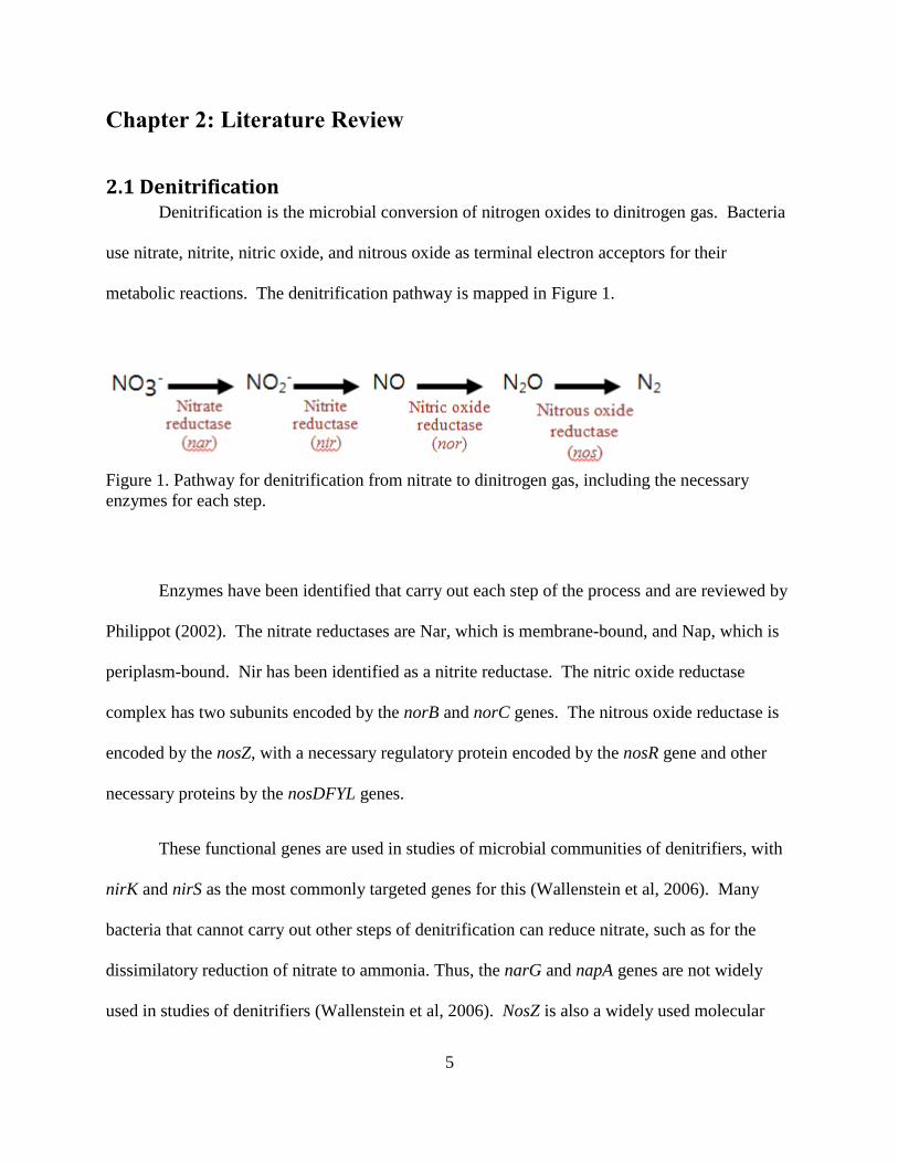
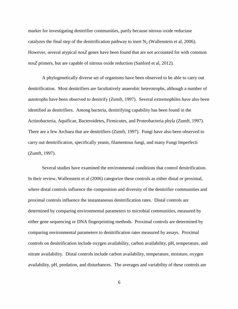
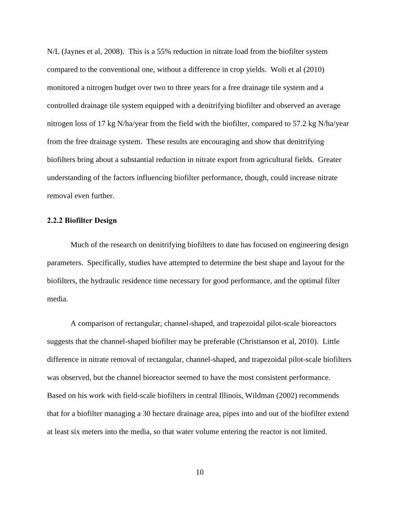
2.1 Denitrification Denitrification is the microbial conversion of nitrogen oxides to dinitrogen gas. Bacteria
use nitrate, nitrite, nitric oxide, and nitrous oxide as terminal electron acceptors for their
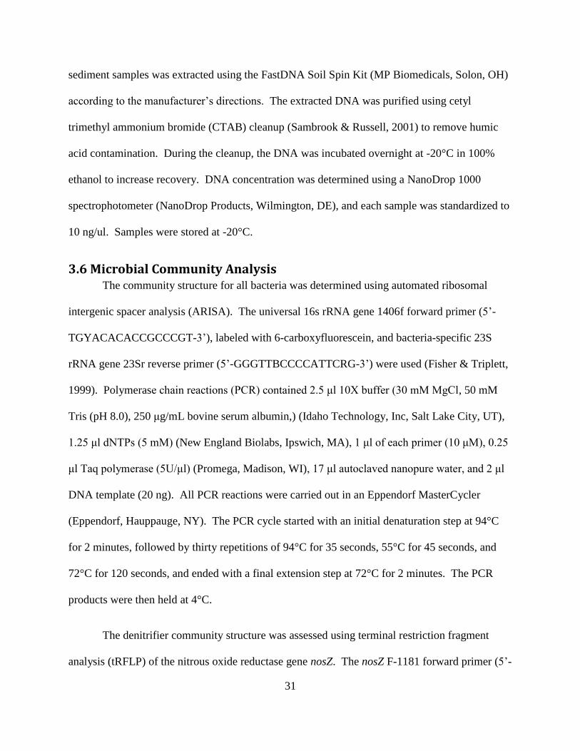
metabolic reactions. The denitrification pathway is mapped in Figure 1.
Figure 1. Pathway for denitrification from nitrate to dinitrogen gas, including the necessary
enzymes for each step.
Enzymes have been identified that carry out each step of the process and are reviewed by
Philippot (2002). The nitrate reductases are Nar, which is membrane-bound, and Nap, which is
periplasm-bound. Nir has been identified as a nitrite reductase. The nitric oxide reductase
complex has two subunits encoded by the norB and norC genes. The nitrous oxide reductase is
encoded by the nosZ, with a necessary regulatory protein encoded by the nosR gene and other
necessary proteins by the nosDFYL genes.
These functional genes are used in studies of microbial communities of denitrifiers, with
nirK and nirS as the most commonly targeted genes for this (Wallenstein et al, 2006). Many
bacteria that cannot carry out other steps of denitrification can reduce nitrate, such as for the
dissimilatory reduction of nitrate to ammonia. Thus, the narG and napA genes are not widely
used in studies of denitrifiers (Wallenstein et al, 2006). NosZ is also a widely used molecular
6
marker for investigating denitrifier communities, partly because nitrous oxide reductase
catalyzes the final step of the denitrification pathway to inert N2 (Wallenstein et al, 2006).
However, several atypical nosZ genes have been found that are not accounted for with common
nosZ primers, but are capable of nitrous oxide reduction (Sanford et al, 2012).
A phylogenetically diverse set of organisms have been observed to be able to carry out
denitrification. Most denitrifiers are facultatively anaerobic heterotrophs, although a number of
autotrophs have been observed to denitrify (Zumft, 1997). Several extremophiles have also been
identified as denitrifiers. Among bacteria, denitrifying capability has been found in the
Actinobacteria, Aquificae, Bacteroidetes, Firmicutes, and Proteobacteria phyla (Zumft, 1997).
There are a few Archaea that are denitrifiers (Zumft, 1997). Fungi have also been observed to
carry out denitrification, specifically yeasts, filamentous fungi, and many Fungi Imperfecti
(Zumft, 1997).
Several studies have examined the environmental conditions that control denitrification.
In their review, Wallenstein et al (2006) categorize these controls as either distal or proximal,
where distal controls influence the composition and diversity of the denitrifier communities and
proximal controls influence the instantaneous denitrification rates. Distal controls are
determined by comparing environmental parameters to microbial communities, measured by
either gene sequencing or DNA fingerprinting methods. Proximal controls are determined by
comparing environmental parameters to denitrification rates measured by assays. Proximal
controls on denitrification include oxygen availability, carbon availability, pH, temperature, and
nitrate availability. Distal controls include carbon availability, temperature, moisture, oxygen
availability, pH, predation, and disturbances. The averages and variability of these controls are
7
also important, in that a consistent temperature is different from a highly variable temperature,
even if the averages are the same.
A consensus has not been reached regarding the relation between denitrifier community
and denitrification enzyme activity. Several studies have found a link between community
composition and denitrification activity. For example, a study comparing the denitrifier
communities and denitrification rates of two geomorphically similar soils found the different
communities to have different denitrification rates under identical incubation conditions as well
as different sensitivity to pH and oxygen (Cavigelli and Roberston, 2000). Similarly, Holtan-
Hartwig et al (2000) compared the denitrification rates of soils from three agricultural fields
under identical laboratory conditions, and found different kinetics for each soil, also suggesting
that the communities influence the denitrification rates. A study of denitrification in streams in
an agricultural area found nosZ gene abundance and T-RF (terminal restriction fragment)
number, determined by redundancy analysis, to be secondary controls on the denitrification rate
in the streams (Baxter et al, 2012).
Other studies, though, have found denitrification rates to be independent of the
denitrifying community composition. A study comparing denitrification activity and nosZ
communities in agricultural soil, riparian soil, and creek sediment found that, although there
were differences in both community composition and nitrous oxide reducing activity, they
appeared uncoupled (Rich and Myrold, 2004). In a reciprocal transplant study, Boyle et al
(2006) a change in denitrification rates after transplanting did not correspond to a change in
microbial communities. Ma et al (2008) were unable to find a link between denitrifying (nosZ)
communities from cultivated and uncultivated wetlands and nitrous oxide production in
laboratory studies.
8
While some studies found a coupling between denitrifier communities and denitrifying
activity, and some did not, it is not clear what determines the difference. Biofilters are
attempting to replicate ecosystem services provided by wetlands, and study of wetlands is likely
the most similar environment to the biofilters. This suggests that a change in community will not
independently bring about a change in activity. Both Rich et al (2003) and Boyle et al (2006)
compared denitrifier communities and activity in forest and meadow soils in Oregon’s Western
Cascade Mountains, though, with opposing conclusions in this regard. Therefore, it does not
appear that the correlation or lack thereof between denitrifier community structure and
denitrification activity in one environment will be a good predictor of the extent of the
correlation in a similar habitat.
9
2.2 Denitrifying Biofilters Several technologies have been proposed to biologically remove nitrate from water
leaving agricultural fields. These technologies include vegetated buffer strips (Osborne &
Kovacic, 1993, Gopalakrishnan et al, 2012), constructed wetlands (Carleton et al, 2001),
denitrification walls (Robertson & Cherry, 1995, Schipper & Vojvodic-Vukovic, 1998), and
denitrifying biofilters (Wildman, 2002, van Driel et al, 2006, Jaynes et al, 2008). In the
literature, denitrifying biofilters are also referred to as denitrification beds, and the term
denitrifying bioreactors includes both denitrifying biofilters and denitrification walls.
Denitrification walls treat groundwater flowing through them, whereas biofilters have influent
and effluent pipes that the water flows through.
This literature review will include studies on the effectiveness of field-scale biofilters,
their design parameters, long-term performance, microbial communities, and greenhouse gas
emissions. The results of many studies on denitrifying walls and biofilters, particularly
laboratory studies, can give insight about the other type of system, so this biofilter-focused
review includes relevant studies on denitrification walls.
2.2.1 Biofilter Effectiveness
Several studies have looked at the effectiveness of denitrifying biofilters under field
conditions and found them to reduce the amount of nitrate exported from agricultural fields. As
reviewed by Schipper et al (2010b), sustained nitrate removal rates under field conditions vary
from 2-22 g N/m3/d, with differences primarily attributed to temperature. A five year
comparison between a denitrifying biofilter, a deep tile drain system, and a conventional
drainage system showed the bioreactor treatments to have an average nitrate concentration of 8.8
mg N/L, whereas the conventional system had 22.1 mg N/L and the deep tile system had 20.5 mg
10
N/L (Jaynes et al, 2008). This is a 55% reduction in nitrate load from the biofilter system
compared to the conventional one, without a difference in crop yields. Woli et al (2010)
monitored a nitrogen budget over two to three years for a free drainage tile system and a
controlled drainage tile system equipped with a denitrifying biofilter and observed an average
nitrogen loss of 17 kg N/ha/year from the field with the biofilter, compared to 57.2 kg N/ha/year
from the free drainage system. These results are encouraging and show that denitrifying
biofilters bring about a substantial reduction in nitrate export from agricultural fields. Greater
understanding of the factors influencing biofilter performance, though, could increase nitrate
removal even further.
2.2.2 Biofilter Design
Much of the research on denitrifying biofilters to date has focused on engineering design
parameters. Specifically, studies have attempted to determine the best shape and layout for the
biofilters, the hydraulic residence time necessary for good performance, and the optimal filter
media.
A comparison of rectangular, channel-shaped, and trapezoidal pilot-scale bioreactors
suggests that the channel-shaped biofilter may be preferable (Christianson et al, 2010). Little
difference in nitrate removal of rectangular, channel-shaped, and trapezoidal pilot-scale biofilters
was observed, but the channel bioreactor seemed to have the most consistent performance.
Based on his work with field-scale biofilters in central Illinois, Wildman (2002) recommends
that for a biofilter managing a 30 hectare drainage area, pipes into and out of the biofilter extend
at least six meters into the media, so that water volume entering the reactor is not limited.
11
Effective nitrate removal has been observed in studies with hydraulic residence time
(HRT) ranging from a few hours to almost ten days. Doheny (2003) suggests a HRT of ten
hours to reduce nitrate in tile drainage with 20-30 mg/L NO3-N to below the EPA limit of 10
mg/L. Greenan et al (2009) also compared bioreactor performance at HRTs of 2.1, 2.8, 3.7, and
9.8 days, but used influent nitrate concentration of 50 mg NO3-N/L, much higher than typically
seen in Illinois tile drainage. At the lowest HRT tested, 2.1 days, a 14.7 mg/L decrease in
nitrate-N concentration was observed, which would decrease the tile drainage concentrations
observed in central Illinois to below the EPA limit. In a study of three pilot-scale biofilters,
observed HRTs were between 1.5 and 2.2 times the theoretical HRTs (Christianson et al, 2011).
The channel-shaped reactor behaved as a plug-flow reactor, and the rectangular and trapezoidal
reactors had higher dispersion. 30-70% nitrate removal from tile drain water with HRTs from 4
to 8 hours was observed.
Several studies have examined different sources of organic carbon to determine the best
filter media for the denitrification walls and denitrifying biofilters. Pine woodchips, eucalyptus
woodchips, sawdust, corn cobs, wheat straw, and green waste were compared in a 23 month
laboratory study, in which corn cobs were associated with the highest nitrate removal rate: 19.8 g
N m-3
d-1
and 15.0 g N m-3
d-1
at 14oC and 23.5
oC, respectively (Cameron and Schipper, 2010).
Ammonium and total Kjeldahl nitrogen were leached from the bioreactors with corn cobs longer
than from the bioreactors with other media. A follow-up study (Warneke et al, 2011) also found
the corn cob treatments to release high concentrations of methane. They suggest that this could
be because the corn cob treatments may be nitrate, rather than carbon limited, allowing
methanogenesis to better compete against denitrification. Although Cameron and Schipper
(2010) found corn cobs to be associated with the highest nitrate removal, Cooke et al (2001)
12
found woodchips to have superior nitrate removal than corn cobs, possibly due to the greater
surface area of the woodchips. Batch tests comparing softwood, hardwood, coniferous, mulch,
willow, compost, and leaves as carbon sources for denitrification found that softwood was
associated with the most efficient denitrification without leaching nitrogen, with hardwood and
coniferous sources also performing well (Gibert et al, 2008). Similarly, Greenan et al (2006)
compared woodchips, woodchips saturated with soybean oil, dried cornstalks, and paper fibers
from corrugated cardboard as a carbon source for denitrification in 180 day batch tests. They
found cornstalks to support the highest degree of nitrate removal, followed by cardboard fibers,
woodchips with oil, and then woodchips alone, but that the nitrate removal rates were steady
with woodchips, and would likely continue longer than with cornstalks. The soybean oil
increased the nitrate removed by 30-70% compared to the woodchips alone. Other media,
including wheat straw (Soares and Abeliovich, 1998) and low quality cotton (Volokita et al,
1996) have also been found effective as a carbon source for denitrification of groundwater, but
have been rapidly degraded.
Comparisons between media of different size shows no difference in nitrate removal rates
for field (van Driel et al, 2006) or laboratory reactors (4-61 mm pine chips) (Cameron and
Schipper, 2010).
2.2.3 Long-term Results
Some studies have observed bioreactors over several years to determine their long-term
performance and the longevity of the media. Long-lasting media is important, because it results
in lower maintenance on the biofilter, thus encouraging their successful implementation.
Moorman et al (2010) observed sustained denitrification potential and nitrate removal from a
13
field biofilter operated for nine years. After that time period, one meter below the surface, 25%
of woodchips remained, and deeper in the biofilter, at least 80% remained. A denitrification wall
with soil-sawdust media was removing 90% of nitrate from the influent after 14 years, and
approximately half of the carbon remained (Long et al, 2011). At this rate of sawdust
degradation, the total carbon in the denitrification wall would not be fully depleted for 66 years,
although that does not indicate when denitrification would become limited by insufficient
accessible carbon. In a sawdust and sand denitrification wall treating a septic system plume with
concentrations as high as 100 mg/L NO3-N, denitrification rates measured during the 15th
year of
operation were about 50% of those measured in the first year (Robertson et al, 2008). Together,
these studies suggest that the longevity of denitrifying biofilters likely depends on local factors,
such as influent nitrate loading, but they can reasonably be expected to remove nitrate for ten
years or more.
2.2.4 Microbial Communities
Microbial communities in denitrifying biofilters have been studied in both field and lab
biofilter environments, but many questions in this area remain unanswered. Porter (2011)
performed a two year temporal study of total bacterial, total fungal, and denitrifying bacterial
communities in three field biofilters. He found the communities to be strongly influenced by
depth and season and that the depth differences were driven by temperature and moisture
gradients. He observed bi-annual seasonal variation in samples, with the greatest distinction
between samples from January-June or July-December. A spatial study of total and denitrifying
bacteria in an L-shaped biofilter was also performed (Andrus, 2011, Porter, 2011). Total
bacterial communities were found to vary by depth and along the flow path, but not orthogonal
to flow-path, but denitrifying bacteria were not found to vary greatly throughout the biofilter.
14
Additionally, a third study looked at the abundance and relative proportions of total
bacteria (16S), nitrite-reducing bacteria (nirS and nirK), and nitrous oxide-reducing bacteria
(nosZ) after 2.5 years in continuously operated laboratory-scale bioreactors with several different
filter media (Warneke et al, 2011). They found pine woodchips to have the lowest denitrification
gene abundance and corn cobs to often have the highest, and that the nitrate removal rate
increases exponentially with nitrite reductase gene abundance. The woodchips, though, had
communities with a higher proportion of nitrite reductase genes making up the total bacterial
communities. They also observed a higher ratio of nitrite reductase genes to nitrous oxide
reductase genes at higher temperatures.
2.2.5 Greenhouse Gas Production
Nitrous oxide, an intermediate in the denitrification pathway, is a potent greenhouse gas
(Forster et al, 2007). There is concern that attempts to remove nitrate using denitrification could
trade a nutrient pollution problem for a climate change one (Groffman et al, 2000). Some studies
have included nitrous oxide measurements in biofilter effluent to be aware of unintended
consequences on air quality. In a study with several laboratory scale bioreactors, nitrous oxide
production accounted for only 0.003-0.028% of the nitrate denitrified, and N2 was the primary
denitrification end product (Greenan et al, 2009). Moorman et al (2010) found lower overall
indirect nitrous oxide emissions from the biofilters than from tile drain water not treated in a
denitrifying biofilter. Denitrifying enzyme assays (DEAs) have been performed on biofilter
samples inhibited and uninhibited by acetylene (Andrus, 2011). Nitrous oxide was below
detection limit in the uninhibited DEAs, indicating that almost all the denitrification proceeded
fully.
15
Research on denitrifying biofilters, to date, has shown them to be an effective technique
for removing nitrate from agricultural drainage, although further improvements are anticipated.
Channel-shaped reactors with woodchip media seem to be the best design for treating tile
drainage. Although greenhouse gas production could be of concern, a few studies have shown
that biofilters do not significantly increase nitrous oxide emissions (Greenan et al, 2009,
Moorman et al, 2010, Andrus, 2011). Studies on the microbial communities of denitrifying
biofilters have indicated that depth and season result in different communities and are correlated
with temperature and moisture gradients (Porter, 2011).
16
2.3 Niche-Legacy Effects Many different factors can have an effect shaping microbial community composition.
These factors can generally be divided between “niche” or “legacy” effects. In ecology, a niche
has a very specific definition, that “an n-dimensional hypervolume is defined, every point in
which corresponds to a state of the environment which would permit the species to exist
indefinitely” (Hutchinson, 1957). For this thesis, a more broad definition of niche will be used,
that a niche is the set of conditions and resources that encourage or discourage the growth of a
species. A community shaped by niche effects has species that have been selected for by the
environmental conditions present at that time. Legacy effects have been defined as the “impacts
of a species on abiotic or biotic features of ecosystems that persist for a long time after the
species has been extirpated or ceased activity and which have an effect on other species”
(Cuddington, 2011). A community shaped by legacy effects contains many species that reflect
the historical conditions of the ecosystem.
In the case of the biofilters being studied, the influent coming into the reactors is coming
from an agricultural field. If the biofilters were colonized and dominated by the microbes
common in the agricultural fields, this would suggest that the legacy effects are central in
shaping the community structure. The biofilters are designed to have wet, anoxic conditions that
encourage denitrification, such as in a wetland. If the microbial communities are similar to those
found in wetlands, it would indicate that the niche effects are governing the structure of the
biofilter’s microbial communities.
It is important to determine whether niche or legacy effects control the composition of
microbial communities in engineered systems. The successful establishment and performance of
17
the biofilters is dependent on the ability of the filter’s conditions to encourage the growth of
denitrifying bacteria, and, to a degree, to approximate the nitrogen removal function of wetlands.
Although few papers specifically address the question of whether niche or legacy effects
dominate in controlling microbial communities, there is a large body of literature that provides
insight on this. This literature review attempts to provide a representative sample of study types
and results that can shed light on this question. First, reciprocal transplant experiments and
common garden experiments will be discussed together, starting with those that suggest legacy
effects, followed by those that suggest niche effects. These will be followed by studies
comparing the microbial communities of similar ecosystems with different land use histories.
The last group of studies to be discussed will be comparisons between communities that have
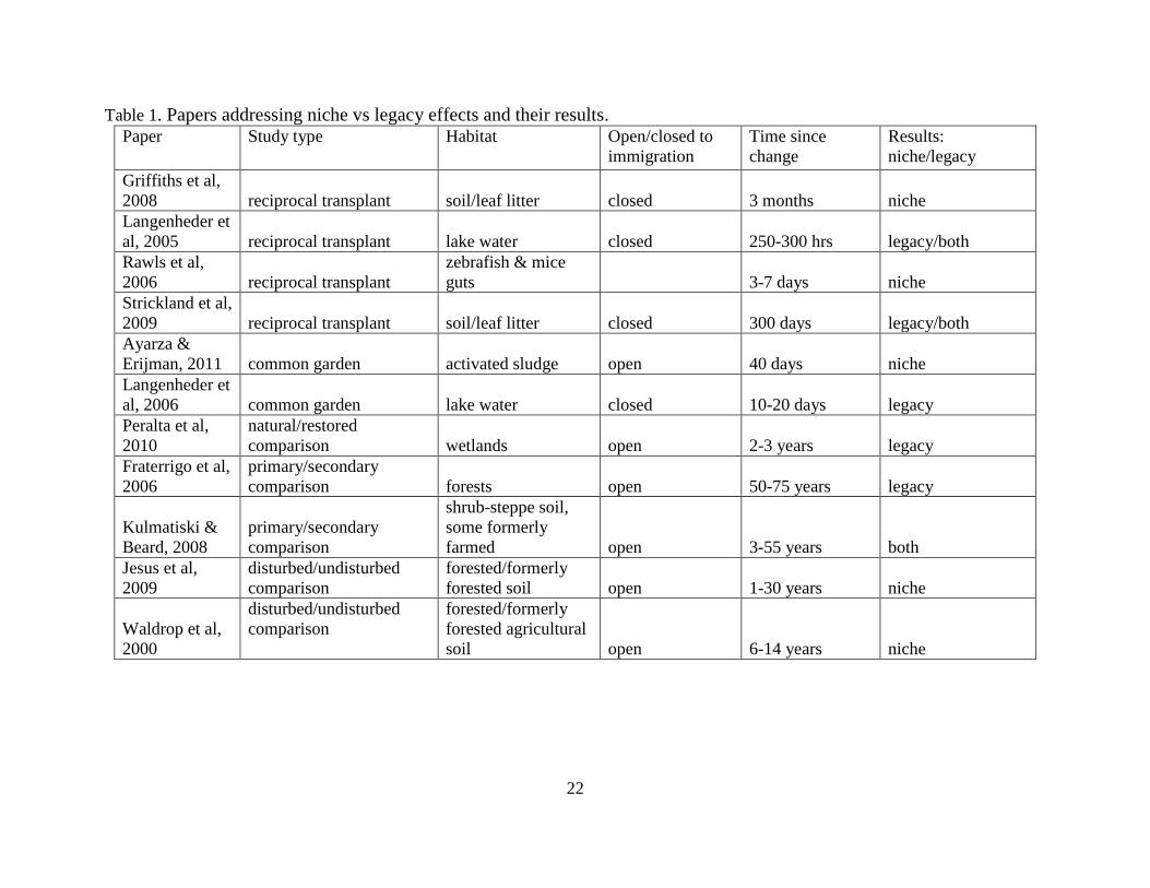
undergone land use change to those that have not been disturbed in this way. Table 1 includes
all the papers included in this literature review, as well as a summary of relevant information and
conclusions, to facilitate comparisons between papers. A discussion of these papers will
conclude this section of the literature review.
Reciprocal transplant studies have been used by several researchers to test the functional
redundancy of microbial communities. This type of experiment involves removing organisms
from one habitat and growing them in another, where organisms from multiple habitats are all
grown separately in each habitat. Similarly, common garden experiments involve growing
organisms from multiple habitats under the same conditions. In some cases, the data collected
on microbial community composition in these studies can also offer insight about the roles of
legacy versus niche in shaping microbial community structure, because the transplanting
represents a disturbance in the communities. If communities change from their original
composition to become like those grown in the same habitat, this indicates a stronger niche
18
effect, whereas, if communities remain more like those from the same original habitat, this
indicates a stronger legacy effect.
In one reciprocal transplant study supporting the importance of legacy effects,
Langenheder et al. (2005) compared bacteria from four different lakes growing in media created
from each lake’s water. The bacterial communities clustered by medium and by inoculum,
indicating that both their current and previous habitat influenced community composition. The
new bacterial communities had between 250 and 300 hours to reach their new structure. If given
more time, the communities might have converged to be more similar to other communities
growing in the same medium. These experiments were closed to migration by outside bacteria.
As a follow up, Langenheder et al. (2006) performed a common garden experiment in
which aquatic bacteria from eight sampling sites with different characteristics were incubated
under identical conditions. The bacterial communities had low similarity between the inoculum
and the community post-incubation. The similarity among the bacterial communities did not
increase from the original inocula to the communities after incubation. These results show a
stronger effect by the initial community than the growth conditions. Again, it may be relevant
that no new bacteria could migrate into the communities, and 10 to 20 days may be insufficient
time for the communities to converge.
Another reciprocal transplant experiment was performed by Strickland et al. (2009), in
which three different types of leaf litter habitat and bacteria from the habitats were crossed with
each other. While both habitat and inoculum showed an effect on the microbial community, the
communities on the same litter habitat did not converge by the end of the 300 day experiment.
19
The communities on the more chemically complex litter habitats came closer to converging than
those on the less complex habitats.
In contrast to the legacy effects observed in the previous studies, Ayarza & Erijman
(2011) set up activated sludge sequencing batch reactors seeded with varying proportions of
different inocula. The reactors were operated in the same manner and received the same
influent. The bacterial communities were functionally stable and converged over time. These
experiments lasted 40 days (10 solids retention times). These reactors were open to the
atmosphere and could receive immigrant populations, so that may be part of why they converged
when the other, closed systems did not.
In a reciprocal transplant study showing the importance of niche effects, Griffiths et al.
(2008) inoculated two types of sterilized soil with bacteria from their own and each other’s
environment. After a three month incubation, the communities in the same types of soil
converged to be more similar to each other than to the communities inoculated with the same
microbial source. These communities were not open to migrant bacteria.
In another reciprocal transplant study, gut microbes from zebrafish and mice were used to
inoculate the digestive tracts of other zebrafish and mice (Rawls et al., 2006). In this case, the
microbial communities in the gut of a particular species are similar to each other, whether they
had grown there since birth or were inoculated from the other species. This study suggests that
the habitat is more important than the legacy in shaping the gut communities.
Studies comparing restored and natural habitats can also offer insight about the relative
effects of legacy versus niche in the structuring of microbial communities. Peralta et al. (2010)
compared bacterial and denitrifier communities in restored and reference wetlands. The bacterial
20
communities of the natural wetlands clustered together, separate from the restored wetlands, as
did the denitrifiers in some cases. This suggests the importance of the legacy of different land
use in shaping community composition.
A similar comparison can be made between primary and secondary communities, as in
Fraterrigo et al (2006). The microbial communities of forests that had been logged, farmed, or
undisturbed 50-75 years prior and since returned to forest were compared. The community
structures were different among each type of site, particularly the farmed site. This was not
explained by differences in the substrate pool or live biomass, suggesting the historic land use
directly influenced the communities. The authors suggest that the farming practices may have
altered the fungi community, which showed the strongest differences among site classifications.
In another comparison between primary and secondary communities, Kulmatiski and
Beard (2008) decoupled the effects of land use legacy and the presence of native versus non-
native plants on soil microbial communities. They sampled soils disturbed by agriculture and
nearby undisturbed soils with native or non-native plants growing on them. There were distinct
soil communities for each treatment, indicating both niche (native vs non-native plants) and
legacy effects. The authors did not address any other potential differences between the disturbed
and undisturbed sites which may be the direct causes of differences in community structure.
Another way to look at the relative effects of niche and legacy is to compare the
microbial communities of formerly similar ecosystems, some of which have undergone land use
changes. Waldrop et al (2000) compared microbial communities in Tahitian pineapple
plantations of different ages in different cultivational stages between each other and nearby
forest. The plantations were cleared and burned between six and fourteen years prior to
21
sampling. The microbial communities from the younger and older plantations were more similar
to each other than they were to the nearby forests. This suggests a niche effect shaping the
microbial communities, rather than the legacy of the previous forest ecosystem.
In a similar set-up, Jesus et al (2009) compared the bacterial communities of formerly
forested soil communities with different land use. Cropped, pasture, agroforestry, young and old
secondary forest, and primary forest sites were included. The microbial communities from each
land use grouped together to varying degrees. They were correlated with different environmental
parameters more than site classification, but the initial similarity of the soils present leads the
authors to conclude that these differences are land use driven. The communities of the secondary
forests were more similar to the primary forest than to the cropped or pasture sites. The
communities from cropped sites were significantly different from the forest communities, even
though they had been converted to cropland within the previous year. This study supports the
idea that these soil communities are influenced more by niche effects than by legacy effects.
22
Table 1. Papers addressing niche vs legacy effects and their results. Paper Study type Habitat Open/closed to
immigration
Time since
change
Results:
niche/legacy
Griffiths et al,
2008 reciprocal transplant soil/leaf litter closed 3 months niche
Langenheder et
al, 2005 reciprocal transplant lake water closed 250-300 hrs legacy/both
Rawls et al,
2006 reciprocal transplant
zebrafish & mice
guts 3-7 days niche
Strickland et al,
2009 reciprocal transplant soil/leaf litter closed 300 days legacy/both
Ayarza &
Erijman, 2011 common garden activated sludge open 40 days niche
Langenheder et
al, 2006 common garden lake water closed 10-20 days legacy
Peralta et al,
2010
natural/restored
comparison wetlands open 2-3 years legacy
Fraterrigo et al,
2006
primary/secondary
comparison forests open 50-75 years legacy
Kulmatiski &
Beard, 2008
primary/secondary
comparison
shrub-steppe soil,
some formerly
farmed open 3-55 years both
Jesus et al,
2009
disturbed/undisturbed
comparison
forested/formerly
forested soil open 1-30 years niche
Waldrop et al,
2000
disturbed/undisturbed
comparison
forested/formerly
forested agricultural
soil open 6-14 years niche
23
A consensus has not been reached regarding the importance of niche versus legacy
effects in shaping microbial communities. Certainly, they both matter to a degree. It is difficult
to separate the effect land use has directly from the effects it has on environmental parameters
that influence community structure. The tropical soils studied by Jesus et al (2009) and Waldrop
et al (2000) may be able to recover more easily than the sites studied by Peralta et al (2010),
Fraterrigo et al (2006) and Kulmatiski et al (2008). The shorter disturbance period caused by
slash-and-burn agriculture may allow for microbial community recovery, whereas sites where
agriculture has been carried out for much longer cannot recover easily.
There were also variable results for the reciprocal transplant experiments. Different
bacteria grow at different rates, and the Langenheder et al (2005, 2006) and Strickland (2009)
experiments might have converged if given more time. It makes sense that the activated sludge
and gut bacteria in Ayarza & Erijman (2011) and Rawls et al (2006) might grow more quickly
given their higher nutrient input. However, this does not explain why the microbial communities
studied by Griffiths et al (2008) converged; perhaps the inocula were more similar to each other
to begin with than in Langenheder et al (2005, 2006) and Strickland (2009).
The habitat in the biofilters is expected to be most like the wetland studied by Peralta et
al (2010), as they both have high moisture content, low dissolved oxygen, and high nitrogen
inputs. As this study found differences in microbial communities and their functioning between
environmentally similar sites with different histories, it reinforces the importance of studying the
relative importance of niche and legacy in the biofilter environment.
24
Chapter 3: Methods
3.1 Reactor Set-up Two laboratory-scale biofilters were previously constructed by Nick Bartolerio, and a
thorough description and schematic can be found in his thesis (Bartolerio, 2011). The biofilters
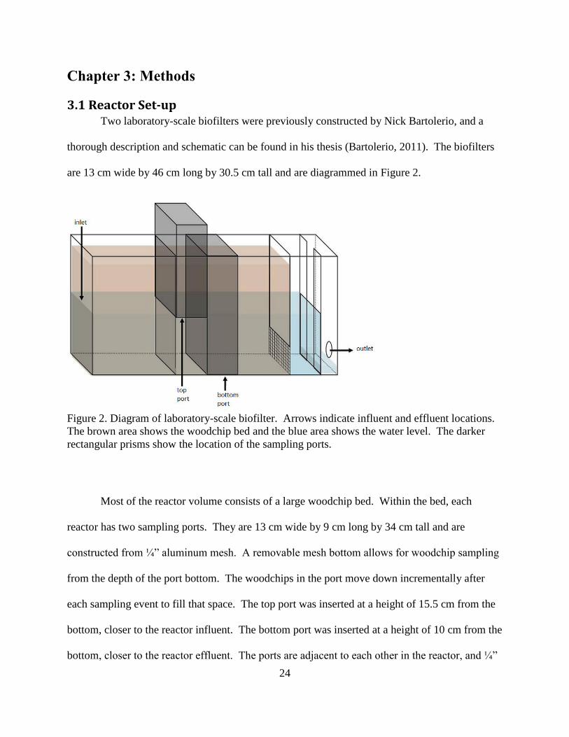
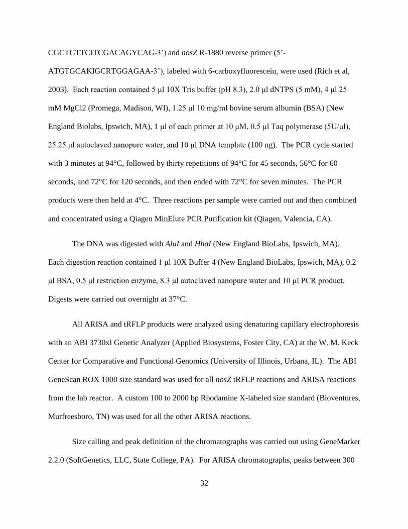
are 13 cm wide by 46 cm long by 30.5 cm tall and are diagrammed in Figure 2.
Figure 2. Diagram of laboratory-scale biofilter. Arrows indicate influent and effluent locations.
The brown area shows the woodchip bed and the blue area shows the water level. The darker
rectangular prisms show the location of the sampling ports.
Most of the reactor volume consists of a large woodchip bed. Within the bed, each
reactor has two sampling ports. They are 13 cm wide by 9 cm long by 34 cm tall and are
constructed from ¼” aluminum mesh. A removable mesh bottom allows for woodchip sampling
from the depth of the port bottom. The woodchips in the port move down incrementally after
each sampling event to fill that space. The top port was inserted at a height of 15.5 cm from the
bottom, closer to the reactor influent. The bottom port was inserted at a height of 10 cm from the
bottom, closer to the reactor effluent. The ports are adjacent to each other in the reactor, and ¼”
25
aluminum mesh separates the area they occupy from the rest of the reactor on either side, to
prevent the woodchips from collapsing when the ports are removed.
At the end of the reactor is the overflow weir/drain compartment. An acrylic baffle wall
extends from the top of the reactor to 5 cm above the bottom and separates this compartment
from the woodchip bed. The area below the baffle wall has ¼” aluminum mesh that prevents
woodchips from the rest of the reactor from getting into the overflow weir/drain compartment.
Water level in the biofilter is controlled by an adjustable overflow weir. Screws through
the effluent side reactor wall hold the weir in place and allow it to be removed.
Tap water was dechlorinated by flowing through an activated carbon column and used as
dilution water. It was mixed with concentrated synthetic tile drainage in a mixing chamber. The
diluted synthetic tile drainage was pumped into the biofilters.
3.2 Reactor Operation The laboratory-scale biofilters were initially filled with woodchips collected from a full-
scale biofilter (FP07) in Decatur, IL. Approximately half of the woodchips came from a
stockpile next to the biofilter and half from the bottom of the biofilter. As woodchips were
depleted from sampling, they were re-stocked with woodchips collected from the stockpile.
The initial woodchip bed porosity at the time of inoculation was 0.60 in the manipulated
reactor and 0.62 in the constant reactor (Bartolerio, 2011).
The reactors were continuously fed with synthetic tile drainage. A basic bacterial and
fungal growth media (Tanner, 1997) was modified to resemble tile drainage for important
constituents. Table 2, Table 3, and Table 4 give the recipe for the feed. A comparison of the

26
composition of the synthetic tile drainage to that of actual tile drainage can be found in
Bartolerio (2011). Influent nitrate concentration was 15 mg NO3--N/L, which is similar to what
would be found in tile drainage in central Illinois (Kalita et al, 2006).
27
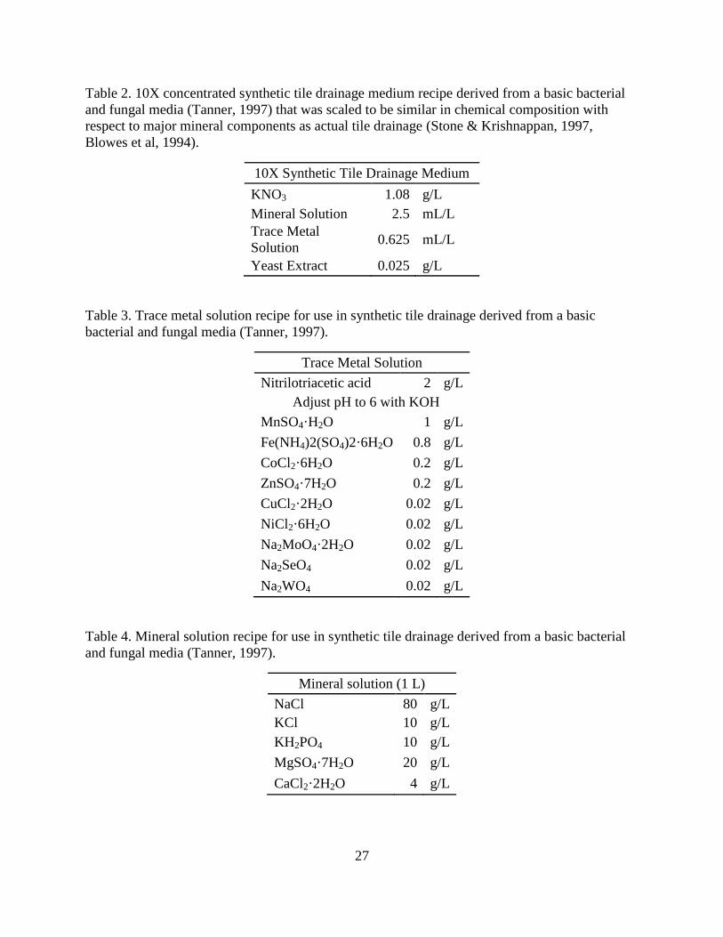
Table 2. 10X concentrated synthetic tile drainage medium recipe derived from a basic bacterial
and fungal media (Tanner, 1997) that was scaled to be similar in chemical composition with
respect to major mineral components as actual tile drainage (Stone & Krishnappan, 1997,
Blowes et al, 1994).
10X Synthetic Tile Drainage Medium
KNO3 1.08 g/L
Mineral Solution 2.5 mL/L
Trace Metal
Solution 0.625 mL/L
Yeast Extract 0.025 g/L
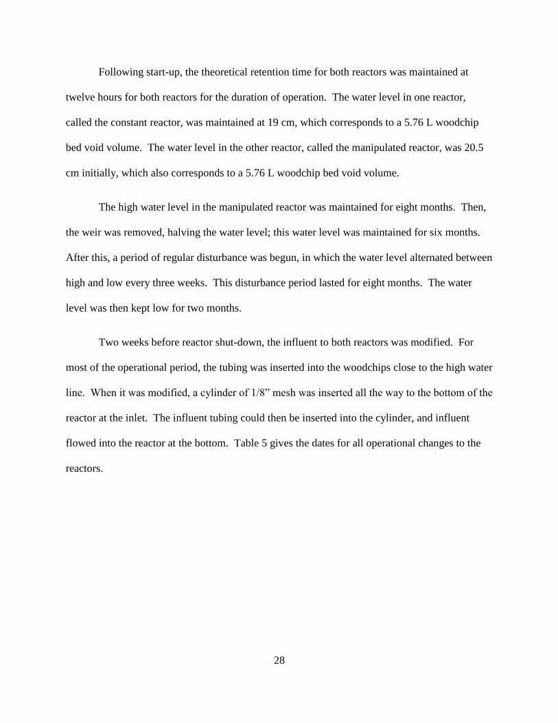
Table 3. Trace metal solution recipe for use in synthetic tile drainage derived from a basic
bacterial and fungal media (Tanner, 1997).
Trace Metal Solution
Nitrilotriacetic acid 2 g/L
Adjust pH to 6 with KOH
MnSO4·H2O 1 g/L
Fe(NH4)2(SO4)2·6H2O 0.8 g/L
CoCl2·6H2O 0.2 g/L
ZnSO4·7H2O 0.2 g/L
CuCl2·2H2O 0.02 g/L
NiCl2·6H2O 0.02 g/L
Na2MoO4·2H2O 0.02 g/L
Na2SeO4 0.02 g/L
Na2WO4 0.02 g/L
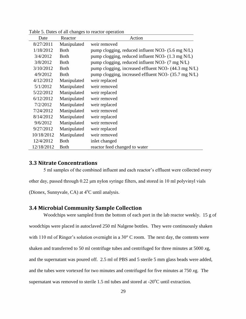
Table 4. Mineral solution recipe for use in synthetic tile drainage derived from a basic bacterial
and fungal media (Tanner, 1997).
Mineral solution (1 L)
NaCl 80 g/L
KCl 10 g/L
KH2PO4 10 g/L
MgSO4·7H2O 20 g/L
CaCl2·2H2O 4 g/L
28
Following start-up, the theoretical retention time for both reactors was maintained at
twelve hours for both reactors for the duration of operation. The water level in one reactor,
called the constant reactor, was maintained at 19 cm, which corresponds to a 5.76 L woodchip
bed void volume. The water level in the other reactor, called the manipulated reactor, was 20.5
cm initially, which also corresponds to a 5.76 L woodchip bed void volume.
The high water level in the manipulated reactor was maintained for eight months. Then,
the weir was removed, halving the water level; this water level was maintained for six months.
After this, a period of regular disturbance was begun, in which the water level alternated between
high and low every three weeks. This disturbance period lasted for eight months. The water
level was then kept low for two months.
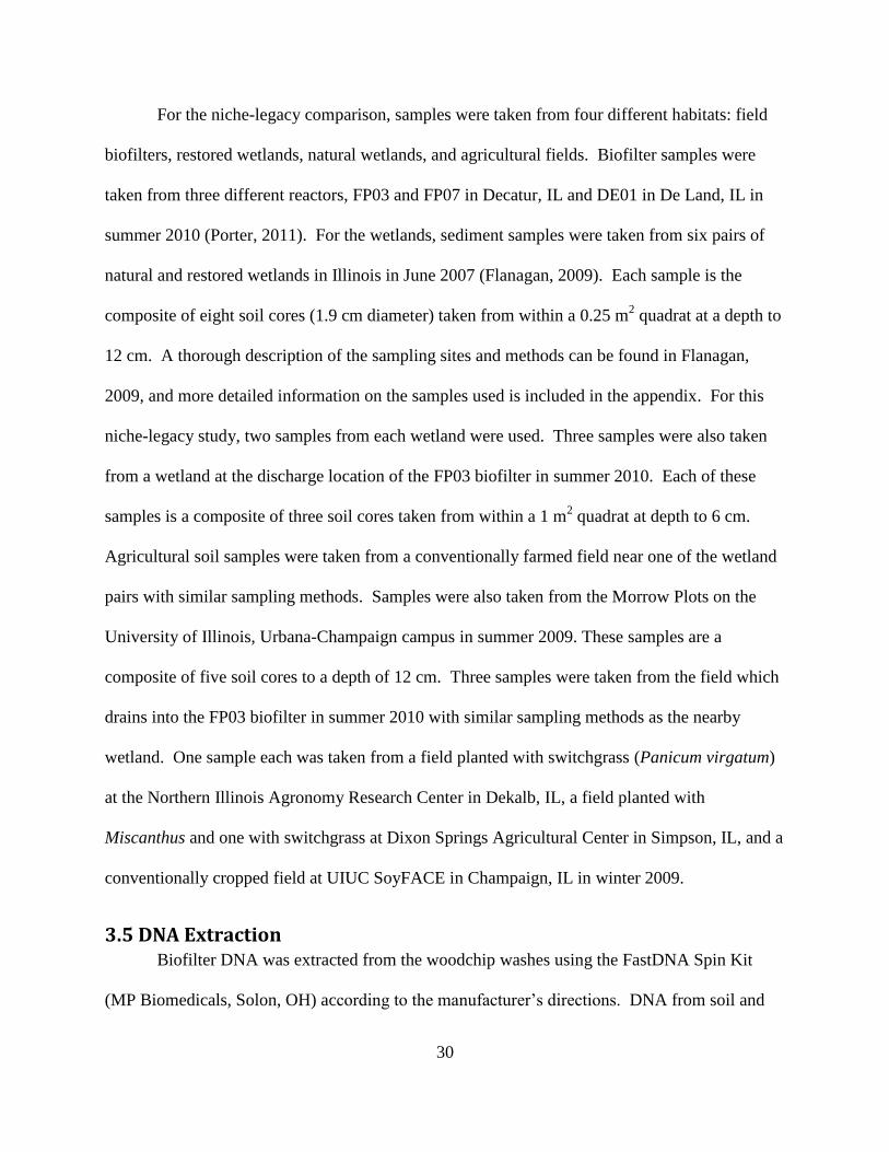
Two weeks before reactor shut-down, the influent to both reactors was modified. For
most of the operational period, the tubing was inserted into the woodchips close to the high water
line. When it was modified, a cylinder of 1/8” mesh was inserted all the way to the bottom of the
reactor at the inlet. The influent tubing could then be inserted into the cylinder, and influent
flowed into the reactor at the bottom. Table 5 gives the dates for all operational changes to the
reactors.
29
Table 5. Dates of all changes to reactor operation
Date Reactor Action
8/27/2011 Manipulated weir removed
1/18/2012 Both pump clogging, reduced influent NO3- (5.6 mg N/L)
3/4/2012 Both pump clogging, reduced influent NO3- (1.3 mg N/L)
3/8/2012 Both pump clogging, reduced influent NO3- (7 mg N/L)
3/10/2012 Both pump clogging, increased effluent NO3- (44.3 mg N/L)
4/9/2012 Both pump clogging, increased effluent NO3- (35.7 mg N/L)
4/12/2012 Manipulated weir replaced
5/1/2012 Manipulated weir removed
5/22/2012 Manipulated weir replaced
6/12/2012 Manipulated weir removed
7/2/2012 Manipulated weir replaced
7/24/2012 Manipulated weir removed
8/14/2012 Manipulated weir replaced
9/6/2012 Manipulated weir removed
9/27/2012 Manipulated weir replaced
10/18/2012 Manipulated weir removed
12/4/2012 Both inlet changed
12/18/2012 Both reactor feed changed to water
3.3 Nitrate Concentrations 5 ml samples of the combined influent and each reactor’s effluent were collected every
other day, passed through 0.22 μm nylon syringe filters, and stored in 10 ml polyvinyl vials
(Dionex, Sunnyvale, CA) at 4oC until analysis.
3.4 Microbial Community Sample Collection Woodchips were sampled from the bottom of each port in the lab reactor weekly. 15 g of
woodchips were placed in autoclaved 250 ml Nalgene bottles. They were continuously shaken
with 110 ml of Ringer’s solution overnight in a 30° C room. The next day, the contents were
shaken and transferred to 50 ml centrifuge tubes and centrifuged for three minutes at 5000 xg,
and the supernatant was poured off. 2.5 ml of PBS and 5 sterile 5 mm glass beads were added,
and the tubes were vortexed for two minutes and centrifuged for five minutes at 750 xg. The
supernatant was removed to sterile 1.5 ml tubes and stored at -20oC until extraction.
30
For the niche-legacy comparison, samples were taken from four different habitats: field
biofilters, restored wetlands, natural wetlands, and agricultural fields. Biofilter samples were
taken from three different reactors, FP03 and FP07 in Decatur, IL and DE01 in De Land, IL in
summer 2010 (Porter, 2011). For the wetlands, sediment samples were taken from six pairs of
natural and restored wetlands in Illinois in June 2007 (Flanagan, 2009). Each sample is the
composite of eight soil cores (1.9 cm diameter) taken from within a 0.25 m2 quadrat at a depth to
12 cm. A thorough description of the sampling sites and methods can be found in Flanagan,
2009, and more detailed information on the samples used is included in the appendix. For this
niche-legacy study, two samples from each wetland were used. Three samples were also taken
from a wetland at the discharge location of the FP03 biofilter in summer 2010. Each of these
samples is a composite of three soil cores taken from within a 1 m2 quadrat at depth to 6 cm.
Agricultural soil samples were taken from a conventionally farmed field near one of the wetland
pairs with similar sampling methods. Samples were also taken from the Morrow Plots on the
University of Illinois, Urbana-Champaign campus in summer 2009. These samples are a
composite of five soil cores to a depth of 12 cm. Three samples were taken from the field which
drains into the FP03 biofilter in summer 2010 with similar sampling methods as the nearby
wetland. One sample each was taken from a field planted with switchgrass (Panicum virgatum)
at the Northern Illinois Agronomy Research Center in Dekalb, IL, a field planted with
Miscanthus and one with switchgrass at Dixon Springs Agricultural Center in Simpson, IL, and a
conventionally cropped field at UIUC SoyFACE in Champaign, IL in winter 2009.
3.5 DNA Extraction Biofilter DNA was extracted from the woodchip washes using the FastDNA Spin Kit
(MP Biomedicals, Solon, OH) according to the manufacturer’s directions. DNA from soil and
31
sediment samples was extracted using the FastDNA Soil Spin Kit (MP Biomedicals, Solon, OH)
according to the manufacturer’s directions. The extracted DNA was purified using cetyl
trimethyl ammonium bromide (CTAB) cleanup (Sambrook & Russell, 2001) to remove humic
acid contamination. During the cleanup, the DNA was incubated overnight at -20°C in 100%
ethanol to increase recovery. DNA concentration was determined using a NanoDrop 1000
spectrophotometer (NanoDrop Products, Wilmington, DE), and each sample was standardized to
10 ng/ul. Samples were stored at -20°C.
3.6 Microbial Community Analysis The community structure for all bacteria was determined using automated ribosomal
intergenic spacer analysis (ARISA). The universal 16s rRNA gene 1406f forward primer (5’-
TGYACACACCGCCCGT-3’), labeled with 6-carboxyfluorescein, and bacteria-specific 23S
rRNA gene 23Sr reverse primer (5’-GGGTTBCCCCATTCRG-3’) were used (Fisher & Triplett,
1999). Polymerase chain reactions (PCR) contained 2.5 μl 10X buffer (30 mM MgCl, 50 mM
Tris (pH 8.0), 250 μg/mL bovine serum albumin,) (Idaho Technology, Inc, Salt Lake City, UT),
1.25 μl dNTPs (5 mM) (New England Biolabs, Ipswich, MA), 1 μl of each primer (10 μM), 0.25
μl Taq polymerase (5U/μl) (Promega, Madison, WI), 17 μl autoclaved nanopure water, and 2 μl
DNA template (20 ng). All PCR reactions were carried out in an Eppendorf MasterCycler
(Eppendorf, Hauppauge, NY). The PCR cycle started with an initial denaturation step at 94°C
for 2 minutes, followed by thirty repetitions of 94°C for 35 seconds, 55°C for 45 seconds, and
72°C for 120 seconds, and ended with a final extension step at 72°C for 2 minutes. The PCR
products were then held at 4°C.
The denitrifier community structure was assessed using terminal restriction fragment
analysis (tRFLP) of the nitrous oxide reductase gene nosZ. The nosZ F-1181 forward primer (5’-
32
CGCTGTTCITCGACAGYCAG-3’) and nosZ R-1880 reverse primer (5’-
ATGTGCAKIGCRTGGAGAA-3’), labeled with 6-carboxyfluorescein, were used (Rich et al,
2003). Each reaction contained 5 μl 10X Tris buffer (pH 8.3), 2.0 μl dNTPS (5 mM), 4 μl 25
mM MgCl2 (Promega, Madison, WI), 1.25 μl 10 mg/ml bovine serum albumin (BSA) (New
England Biolabs, Ipswich, MA), 1 μl of each primer at 10 μM, 0.5 μl Taq polymerase (5U/μl),
25.25 μl autoclaved nanopure water, and 10 μl DNA template (100 ng). The PCR cycle started
with 3 minutes at 94°C, followed by thirty repetitions of 94°C for 45 seconds, 56°C for 60
seconds, and 72°C for 120 seconds, and then ended with 72°C for seven minutes. The PCR
products were then held at 4°C. Three reactions per sample were carried out and then combined
and concentrated using a Qiagen MinElute PCR Purification kit (Qiagen, Valencia, CA).
The DNA was digested with AluI and HhaI (New England BioLabs, Ipswich, MA).
Each digestion reaction contained 1 μl 10X Buffer 4 (New England BioLabs, Ipswich, MA), 0.2
μl BSA, 0.5 μl restriction enzyme, 8.3 μl autoclaved nanopure water and 10 μl PCR product.
Digests were carried out overnight at 37°C.
All ARISA and tRFLP products were analyzed using denaturing capillary electrophoresis
with an ABI 3730xl Genetic Analyzer (Applied Biosystems, Foster City, CA) at the W. M. Keck
Center for Comparative and Functional Genomics (University of Illinois, Urbana, IL). The ABI
GeneScan ROX 1000 size standard was used for all nosZ tRFLP reactions and ARISA reactions
from the lab reactor. A custom 100 to 2000 bp Rhodamine X-labeled size standard (Bioventures,
Murfreesboro, TN) was used for all the other ARISA reactions.
Size calling and peak definition of the chromatographs was carried out using GeneMarker
2.2.0 (SoftGenetics, LLC, State College, PA). For ARISA chromatographs, peaks between 300
33
and 1000 base pairs were included, and a minimum fluorescence threshold of 200 was used. For
nosZ tRFLP chromatographs, peaks between 100 and 700 base pairs were included, and a
minimum fluorescence threshold of 80 was used. The minimum and maximum size for each
peak was defined using the allele calling features in GeneMarker. Each peak is considered to
represent a distinct operational taxonomic unit (OTU).
3.7 Microbial Community Statistical Analysis Lab reactor microbial communities were analyzed using PRIMER 6, version 6.1.10
(Primer-E, Ltd., Plymouth, UK). Non-metric multi-dimensional scaling (MDS) plots were
generated to visually analyze the patterns in microbial community structure. The ANOSIM
function (Clarke and Green, 1988) was used to generate similarity values among different groups
of samples. The DIVERSE function was used to determine species richness.
Partial correspondence analysis was used for the niche-legacy comparison using Canoco
for Windows 4.5.1 (Plant Research International, Wageningen, Netherlands) (ter Braak et al,
2002). The environmental variables used were moisture and habitat categorization as biofilter,
natural wetland, restored wetland, or agriculture. The influence of location was removed from
the analysis with latitude and longitude as covariables. The program parameters used were
species, environment, and covariable data available; indirect gradient; unimodal (CA) response;
inter-sample distances; biplot scaling; and no transformation of species data.
3.8 Denitrification Potential Denitrification potential was measured through denitrification enzyme assays (DEA) with
the acetylene block method (Tiedje et al, 1989). These assays were performed in duplicate for
each sampling port. Ten grams of woodchips were incubated in a Wheaton bottle with 75 ml of
solution containing 15 mg/L NO3- and 0.1 g chloramphenicol. The chloramphenicol prevents the
34
bacteria from synthesizing new protein, so only enzymes that are already present contribute to
the denitrification potential. In selected assays, 1 mM glucose was included. The headspace was
flushed with helium gas, and acetylene gas added to achieve a headspace concentration of about
20%. Acetylene prevents the final denitrification step from nitrous oxide to dinitrogen gas.
Samples were taken at times zero, two, four, and six hours. Gas samples were taken and stored
in 10 ml Vacutainers (BD, Franklin Lakes, NJ). Liquid samples were filtered with 0.22 μl
syringe filters and stored in 10 ml polyvinyl vials (Dionex, Sunnyvale, CA). After each
sampling point, the extracted volume was replaced with 10:1 helium: acetylene gas mix. The
Vacutainers had silicon sealant spread on the top to prevent contamination. The liquid samples
were stored at 4°C until analysis. After the assay, the headspace volume was measured, and the
bottles were placed in a drying oven at 105°C to determine the dry weight of woodchips.
The nitrate concentrations were converted to total nitrate removed from the bottle. A
linear regression of this was used to calculate the rate of nitrate removal, where the slope of the
regression line is the mass of nitrate removed per hour. The t0 sample was not included in the
regression, because it was usually not linear with the other time points. The nitrate removal rates
were normalized per dry gram of woodchips.
The nitrous oxide concentrations were converted to total N2O produced in the bottle.
Similarly to nitrate removal, a linear regression was used to calculate the rate of nitrous oxide
produced per hour. This rate was also normalized per dry gram of woodchips.
3.9 Statistical Analysis of Denitrification Potential The denitrification potential values for multiple categories of disturbance and water level
were averaged together. Significance of values was evaluated using paired t-tests for unequal
variance in Microsoft Excel (Microsoft Corporation, Redmond, WA).
35
3.10 Tracer Studies Tracer studies were performed on both reactors, twice with the changed inlet and twice
with the original inlet. The manipulated reactor had a low water level during all the tracer
studies. The first set of tracer studies took place in early December 2012, shortly before reactor
shut down. The second set of tracer studies were performed because of problems with analysis
of the first set of tracer studies. They took place six months after reactor shut down;
dechlorinated water had been flowing through the reactors, but no nutrient feed. They are
compared to tracer studies performed on the reactors by Nick Bartolerio (2011) in November
2011, when the manipulated reactor was being subjected to its extended low water period and the
inlet had not been modified.
A step input of 100 ppm bromide was used as the tracer. Effluent samples were taken
every hour for the first five hours, every half hour for the next thirteen hours, and every hour for
the remaining eighteen hours.
The cumulative residence time distribution, F(t), given in equation 1below, was
determined from the effluent bromide concentrations.
( ) ( )
(1)
where ceff(t) = effluent bromide concentration at time t
co = influent bromide concentration
The derivitive of F(t) is the residence time density function, f(t). The mean residence
time, t, is computed from f(t) according to equation 2.
∫ ( )
(2)
36
f(t) at the sampling time j was approximated using equation 3.
( ) (
) ( ) ( )
(3)
The mean residence time could then be approximated according to equation 4.
∑ ( ) (
)( )
∑ ( ) ( )
(4)
3.11 Dissolved Oxygen Measurements Dissolved oxygen was measured with a YSI Professional Plus handheld multiparameter
meter with Quattro cable and probe 1003 (pH/ORP) (YSI, Yellow Springs, OH). Measurements
were taken twice in each port of the reactor, once at low water level on September 28, 2012 and
once at high water level on October 2, 2012. Because the top port of the manipulated reactor
was not submerged at low water level, dissolved oxygen could not be measured in that port then.
To allow the probe into the reactor, the sampling ports were removed when taking the
measurements. Readings were taken as quickly as possible after removing the sampling port, but
removing the port may have introduced some oxygen.
3.12 Analytical Measurements Gas samples taken during the DEAs were analyzed using a Shimadzu GC-2014AFsc gas
chromatography system with packed columns and GCSolution software (Shimadzu Corporation,
Nakagyo-ku, Kyoto, Japan). Preconditioned, custom packed HayeSep N 80-100 columns were
included in the set-up (Supelco, Bellefonte, PA). A standard curve was created for each run
using standards with 0.11 ppm, 0.73 ppm, 1.09 ppm, 1.80 ppm, 3.67 ppm, and 7.33 ppm N2O.
37
Liquid samples taken during the DEAs and for reactor performance were analyzed for
nitrate concentration using an ICS-2000 ion chromatography system with Chromeleon
Chromatography Management Software (Dionex, Sunnyvale, CA). An IonPac AS18 4x250 mm
hydroxide-selective anion-exchange column was used in the set-up. A standard curve was
created for each run using standards with 3.125 ppm, 6.25 ppm, 12.5 ppm, 25 ppm, 50 ppm, and
100 ppm NO3-. Samples taken during the tracer studies were analyzed for bromide this way,
also. The same concentrations were used for the bromide standards as for the nitrate standards.
38
Chapter 4: Results of Laboratory Biofilter Study
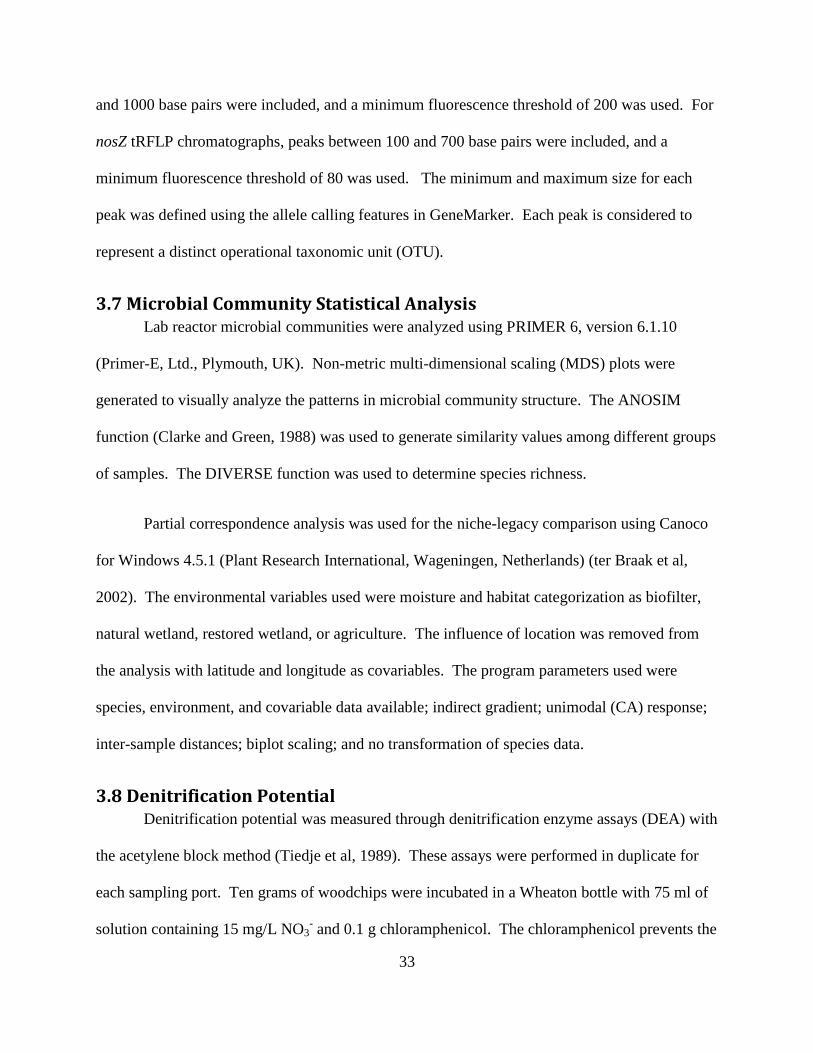
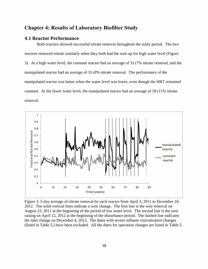
4.1 Reactor Performance Both reactors showed successful nitrate removal throughout the study period. The two
reactors removed nitrate similarly when they both had the weir up for high water level (Figure
3). At a high water level, the constant reactor had an average of 31±7% nitrate removal, and the
manipulated reactor had an average of 31±8% nitrate removal. The performance of the
manipulated reactor was better when the water level was lower, even though the HRT remained
constant. At the lower water level, the manipulated reactor had an average of 59±11% nitrate
removal.
Figure 3. 5-day average of nitrate removal by each reactor from April 3, 2011 to December 18,
2012. The solid vertical lines indicate a weir change. The first line is the weir removal on
August 23, 2011 at the beginning of the period of low water level. The second line is the weir
raising on April 12, 2012 at the beginning of the disturbance period. The dashed line indicates
the inlet change on December 4, 2012. The dates with severe influent concentration changes
(listed in Table 5.) have been excluded. All the dates for operation changes are listed in Table 5.
39
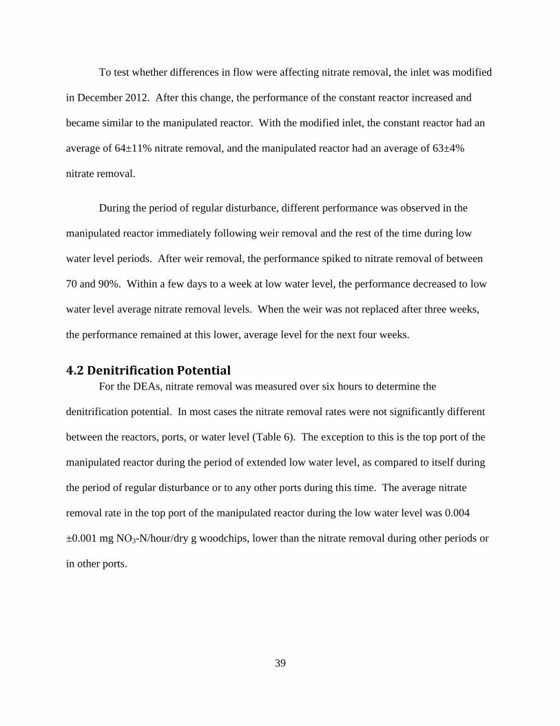
To test whether differences in flow were affecting nitrate removal, the inlet was modified
in December 2012. After this change, the performance of the constant reactor increased and
became similar to the manipulated reactor. With the modified inlet, the constant reactor had an
average of 64±11% nitrate removal, and the manipulated reactor had an average of 63±4%
nitrate removal.
During the period of regular disturbance, different performance was observed in the
manipulated reactor immediately following weir removal and the rest of the time during low
water level periods. After weir removal, the performance spiked to nitrate removal of between
70 and 90%. Within a few days to a week at low water level, the performance decreased to low
water level average nitrate removal levels. When the weir was not replaced after three weeks,
the performance remained at this lower, average level for the next four weeks.
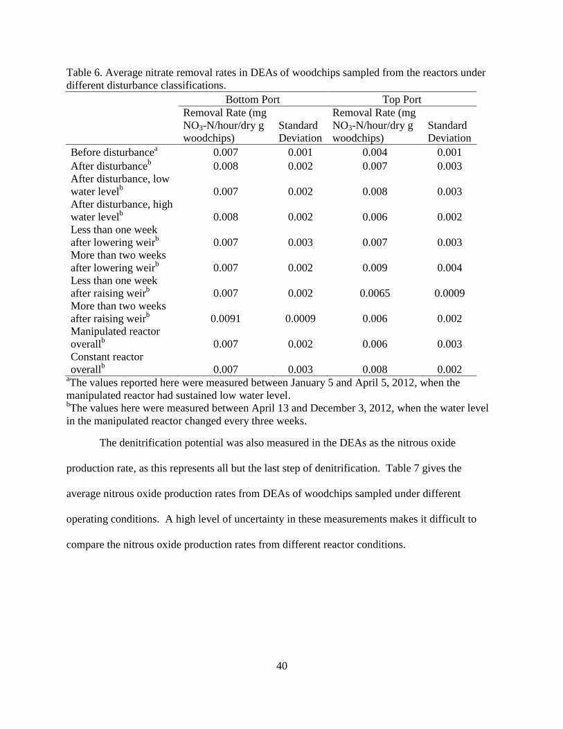
4.2 Denitrification Potential For the DEAs, nitrate removal was measured over six hours to determine the
denitrification potential. In most cases the nitrate removal rates were not significantly different
between the reactors, ports, or water level (Table 6). The exception to this is the top port of the
manipulated reactor during the period of extended low water level, as compared to itself during
the period of regular disturbance or to any other ports during this time. The average nitrate
removal rate in the top port of the manipulated reactor during the low water level was 0.004
±0.001 mg NO3-N/hour/dry g woodchips, lower than the nitrate removal during other periods or
in other ports.
40
Table 6. Average nitrate removal rates in DEAs of woodchips sampled from the reactors under
different disturbance classifications.
Bottom Port Top Port
Removal Rate (mg
NO3-N/hour/dry g
woodchips)
Standard
Deviation
Removal Rate (mg
NO3-N/hour/dry g
woodchips)
Standard
Deviation
Before disturbancea 0.007 0.001 0.004 0.001
After disturbanceb 0.008 0.002 0.007 0.003
After disturbance, low
water levelb 0.007 0.002 0.008 0.003
After disturbance, high
water levelb 0.008 0.002 0.006 0.002
Less than one week
after lowering weirb 0.007 0.003 0.007 0.003
More than two weeks
after lowering weirb 0.007 0.002 0.009 0.004
Less than one week
after raising weirb 0.007 0.002 0.0065 0.0009
More than two weeks
after raising weirb 0.0091 0.0009 0.006 0.002
Manipulated reactor
overallb 0.007 0.002 0.006 0.003
Constant reactor
overallb 0.007 0.003 0.008 0.002
aThe values reported here were measured between January 5 and April 5, 2012, when the
manipulated reactor had sustained low water level. bThe values here were measured between April 13 and December 3, 2012, when the water level
in the manipulated reactor changed every three weeks.
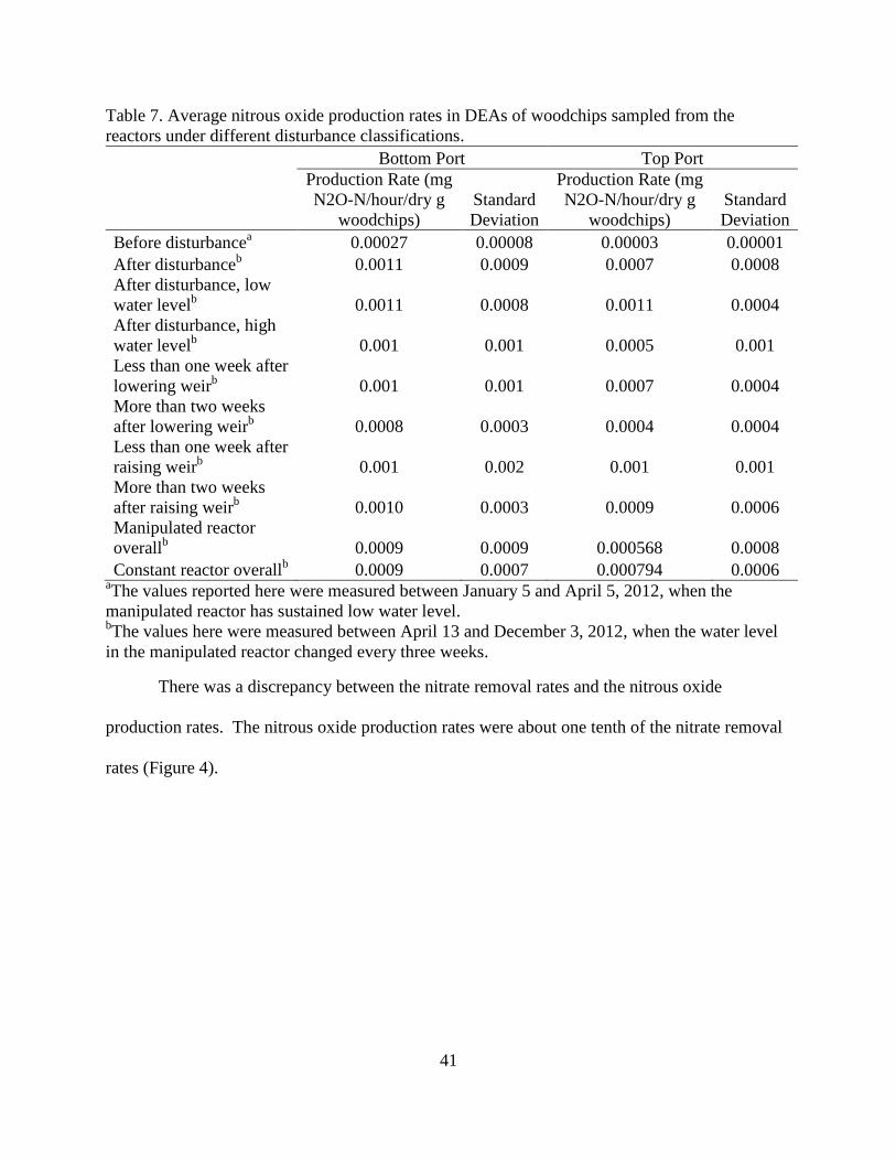
The denitrification potential was also measured in the DEAs as the nitrous oxide
production rate, as this represents all but the last step of denitrification. Table 7 gives the
average nitrous oxide production rates from DEAs of woodchips sampled under different
operating conditions. A high level of uncertainty in these measurements makes it difficult to
compare the nitrous oxide production rates from different reactor conditions.
41
Table 7. Average nitrous oxide production rates in DEAs of woodchips sampled from the
reactors under different disturbance classifications.
Bottom Port Top Port
Production Rate (mg
N2O-N/hour/dry g
woodchips)
Standard
Deviation
Production Rate (mg
N2O-N/hour/dry g
woodchips)
Standard
Deviation
Before disturbancea 0.00027 0.00008 0.00003 0.00001
After disturbanceb 0.0011 0.0009 0.0007 0.0008
After disturbance, low
water levelb 0.0011 0.0008 0.0011 0.0004
After disturbance, high
water levelb 0.001 0.001 0.0005 0.001
Less than one week after
lowering weirb 0.001 0.001 0.0007 0.0004
More than two weeks
after lowering weirb 0.0008 0.0003 0.0004 0.0004
Less than one week after
raising weirb 0.001 0.002 0.001 0.001
More than two weeks
after raising weirb 0.0010 0.0003 0.0009 0.0006
Manipulated reactor
overallb 0.0009 0.0009 0.000568 0.0008
Constant reactor overallb 0.0009 0.0007 0.000794 0.0006
aThe values reported here were measured between January 5 and April 5, 2012, when the
manipulated reactor has sustained low water level. bThe values here were measured between April 13 and December 3, 2012, when the water level
in the manipulated reactor changed every three weeks.
There was a discrepancy between the nitrate removal rates and the nitrous oxide
production rates. The nitrous oxide production rates were about one tenth of the nitrate removal
rates (Figure 4).
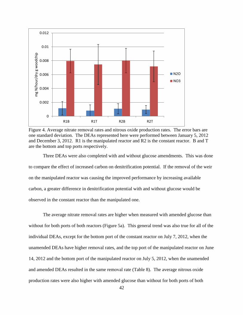
42
Figure 4. Average nitrate removal rates and nitrous oxide production rates. The error bars are
one standard deviation. The DEAs represented here were performed between January 5, 2012
and December 3, 2012. R1 is the manipulated reactor and R2 is the constant reactor. B and T
are the bottom and top ports respectively.
Three DEAs were also completed with and without glucose amendments. This was done
to compare the effect of increased carbon on denitrification potential. If the removal of the weir
on the manipulated reactor was causing the improved performance by increasing available
carbon, a greater difference in denitrification potential with and without glucose would be
observed in the constant reactor than the manipulated one.
The average nitrate removal rates are higher when measured with amended glucose than
without for both ports of both reactors (Figure 5a). This general trend was also true for all of the
individual DEAs, except for the bottom port of the constant reactor on July 7, 2012, when the
unamended DEAs have higher removal rates, and the top port of the manipulated reactor on June
14, 2012 and the bottom port of the manipulated reactor on July 5, 2012, when the unamended
and amended DEAs resulted in the same removal rate (Table 8). The average nitrous oxide
production rates were also higher with amended glucose than without for both ports of both
0
0.002
0.004
0.006
0.008
0.01
0.012
R1B R1T R2B R2T
mg
N/h
ou
r/d
ry g
wo
od
chip
N2O
NO3
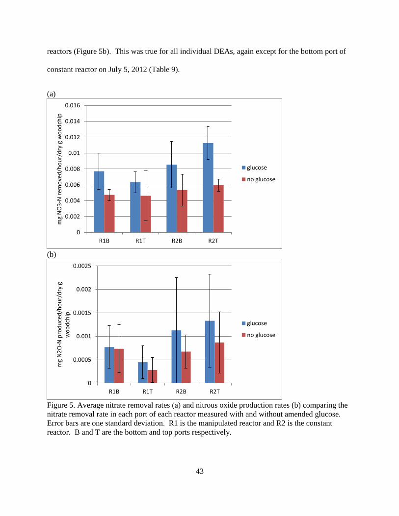
43
reactors (Figure 5b). This was true for all individual DEAs, again except for the bottom port of
constant reactor on July 5, 2012 (Table 9).
(a)
(b)
Figure 5. Average nitrate removal rates (a) and nitrous oxide production rates (b) comparing the
nitrate removal rate in each port of each reactor measured with and without amended glucose.
Error bars are one standard deviation. R1 is the manipulated reactor and R2 is the constant
reactor. B and T are the bottom and top ports respectively.
0
0.002
0.004
0.006
0.008
0.01
0.012
0.014
0.016
R1B R1T R2B R2T
mg
NO
3-N
rem
ove
d/h
ou
r/d
ry g
wo
od
chip
glucose
no glucose
0
0.0005
0.001
0.0015
0.002
0.0025
R1B R1T R2B R2T
mg
N2
O-N
pro
du
ced
/ho
ur/
dry
g
wo
od
chip
glucose
no glucose
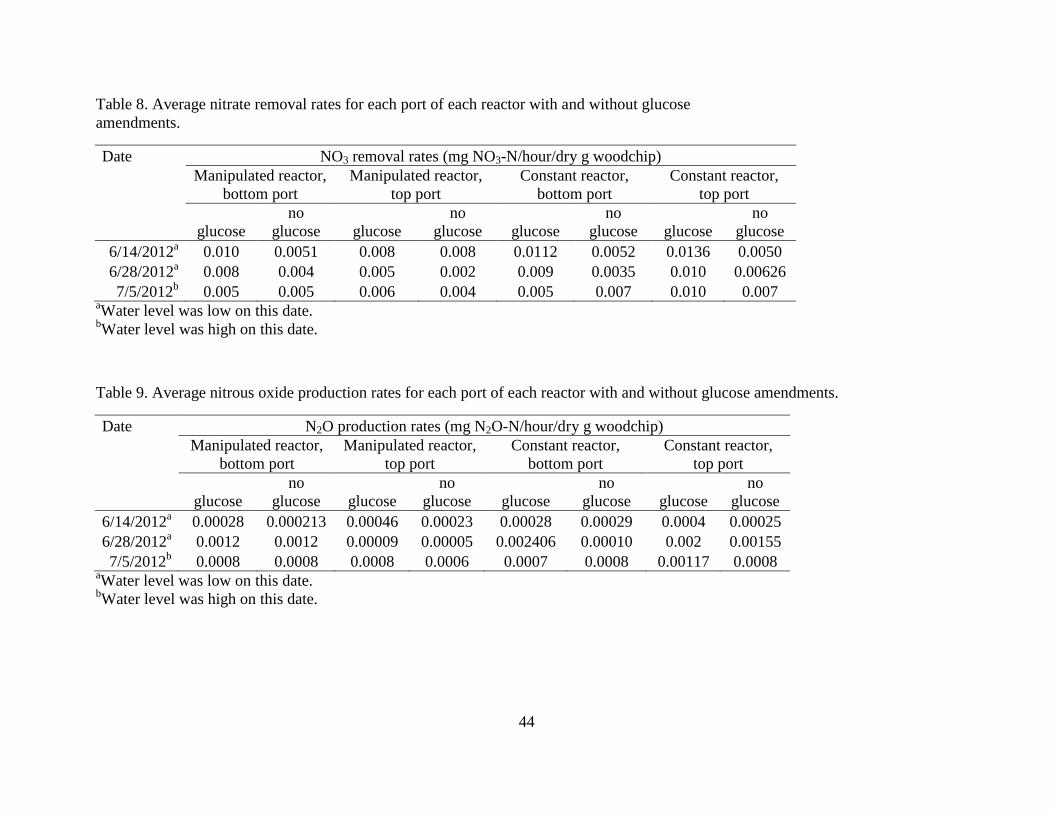
44
Table 8. Average nitrate removal rates for each port of each reactor with and without glucose
amendments.
Date NO3 removal rates (mg NO3-N/hour/dry g woodchip)
Manipulated reactor,
bottom port
Manipulated reactor,
top port
Constant reactor,
bottom port
Constant reactor,
top port
glucose
no
glucose glucose
no
glucose glucose
no
glucose glucose
no
glucose
6/14/2012a 0.010 0.0051 0.008 0.008 0.0112 0.0052 0.0136 0.0050
6/28/2012a 0.008 0.004 0.005 0.002 0.009 0.0035 0.010 0.00626
7/5/2012b 0.005 0.005 0.006 0.004 0.005 0.007 0.010 0.007
aWater level was low on this date.
bWater level was high on this date.
Table 9. Average nitrous oxide production rates for each port of each reactor with and without glucose amendments.
Date N2O production rates (mg N2O-N/hour/dry g woodchip)
Manipulated reactor,
bottom port
Manipulated reactor,
top port
Constant reactor,
bottom port
Constant reactor,
top port
glucose
no
glucose glucose
no
glucose glucose
no
glucose glucose
no
glucose
6/14/2012a 0.00028 0.000213 0.00046 0.00023 0.00028 0.00029 0.0004 0.00025
6/28/2012a 0.0012 0.0012 0.00009 0.00005 0.002406 0.00010 0.002 0.00155
7/5/2012b 0.0008 0.0008 0.0008 0.0006 0.0007 0.0008 0.00117 0.0008
aWater level was low on this date.
bWater level was high on this date.
45
Similarly to the unamended DEAs, the nitrate removal rates in the glucose-amended
DEAs were about ten times higher than the nitrous oxide production rates.
4.3 Microbial Community Composition My study on microbial community composition in the lab reactors focused on the effect
of changing water level on the bacterial communities. How do the communities respond to
regular disturbance: does it result in different OTUs? How is overall diversity affected? How do
different parts of the reactor respond to the changing water level? Ideally, a comparison between
the microbial communities and the performance of the reactors will also be possible.
4.3.1 Total Bacterial Communities
The analysis of total bacterial communities included 317 unique OTUs. Each sample
contained between four and 123 OTUs, with a median of 70. The median number of OTUs was
similar for both reactors.
The total bacterial communities in the manipulated reactor were similar to those in the
same port, regardless of water level (Figure 6). ANOSIM R values are used to evaluate the
similarity of different classifications of samples (eg. manipulated vs. constant reactor). A value
close to 0 means that the samples are similar to each other, and a value close to 1 indicates that
they are dissimilar. An insignificant ANOSIM R value indicates that the groups of communities
being compared are indistinct from each other. The ANOSIM R value comparing the top port
communities at low and high water levels was not significant, nor was the value comparing the
bottom port communities at low and high water levels, meaning that the communities are not
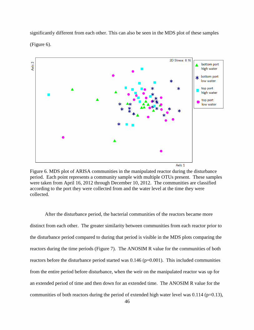
46
significantly different from each other. This can also be seen in the MDS plot of these samples
(Figure 6).
Figure 6. MDS plot of ARISA communities in the manipulated reactor during the disturbance
period. Each point represents a community sample with multiple OTUs present. These samples
were taken from April 16, 2012 through December 10, 2012. The communities are classified
according to the port they were collected from and the water level at the time they were
collected.
After the disturbance period, the bacterial communities of the reactors became more
distinct from each other. The greater similarity between communities from each reactor prior to
the disturbance period compared to during that period is visible in the MDS plots comparing the
reactors during the time periods (Figure 7). The ANOSIM R value for the communities of both
reactors before the disturbance period started was 0.146 (p=0.001). This included communities
from the entire period before disturbance, when the weir on the manipulated reactor was up for
an extended period of time and then down for an extended time. The ANOSIM R value for the
communities of both reactors during the period of extended high water level was 0.114 (p=0.13),
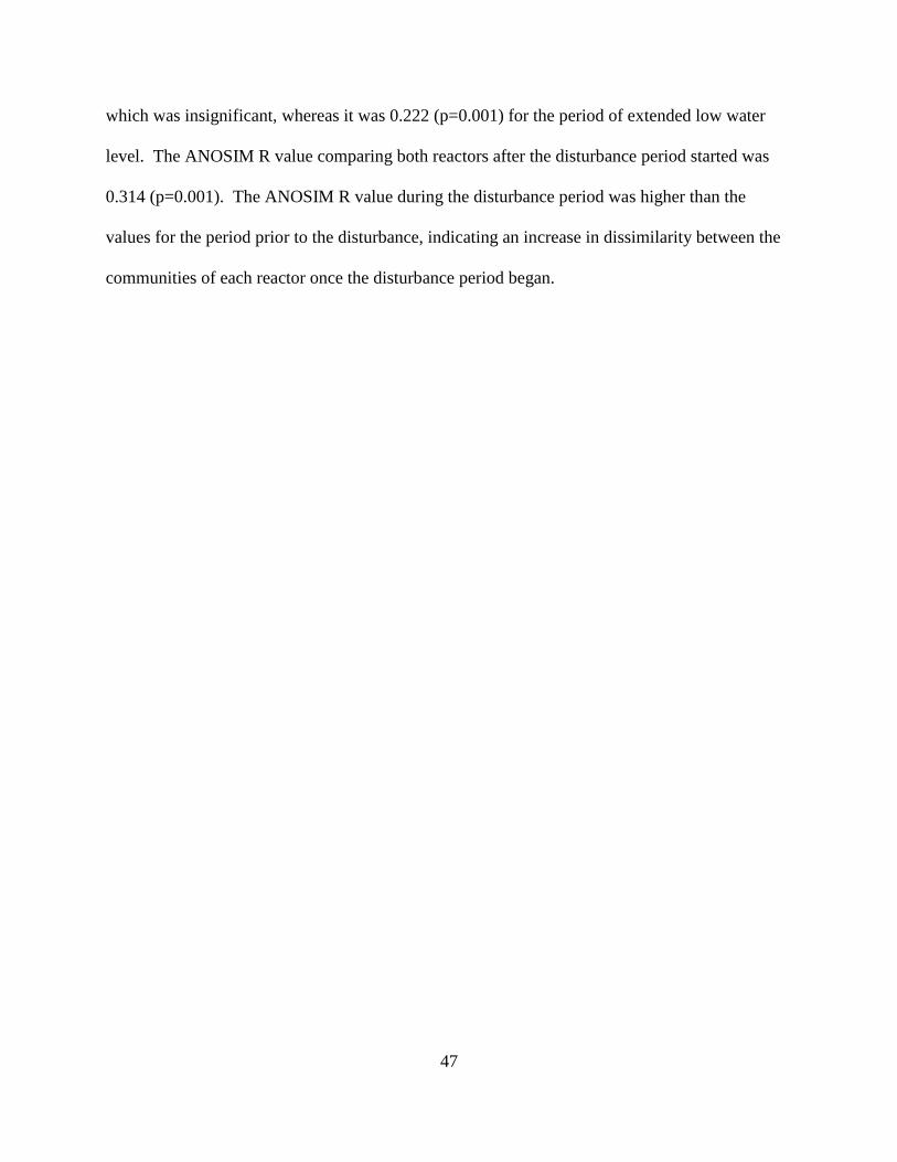
47
which was insignificant, whereas it was 0.222 (p=0.001) for the period of extended low water
level. The ANOSIM R value comparing both reactors after the disturbance period started was
0.314 (p=0.001). The ANOSIM R value during the disturbance period was higher than the
values for the period prior to the disturbance, indicating an increase in dissimilarity between the
communities of each reactor once the disturbance period began.
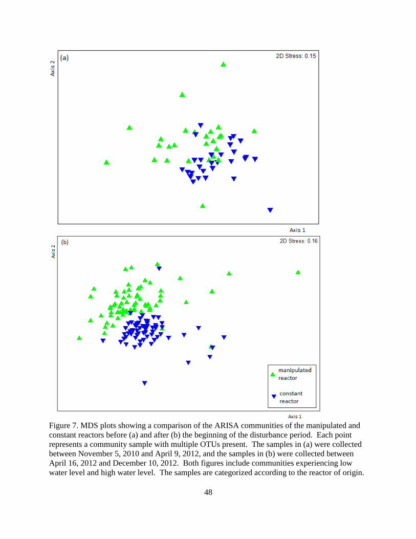
48
Figure 7. MDS plots showing a comparison of the ARISA communities of the manipulated and
constant reactors before (a) and after (b) the beginning of the disturbance period. Each point
represents a community sample with multiple OTUs present. The samples in (a) were collected
between November 5, 2010 and April 9, 2012, and the samples in (b) were collected between
April 16, 2012 and December 10, 2012. Both figures include communities experiencing low
water level and high water level. The samples are categorized according to the reactor of origin.
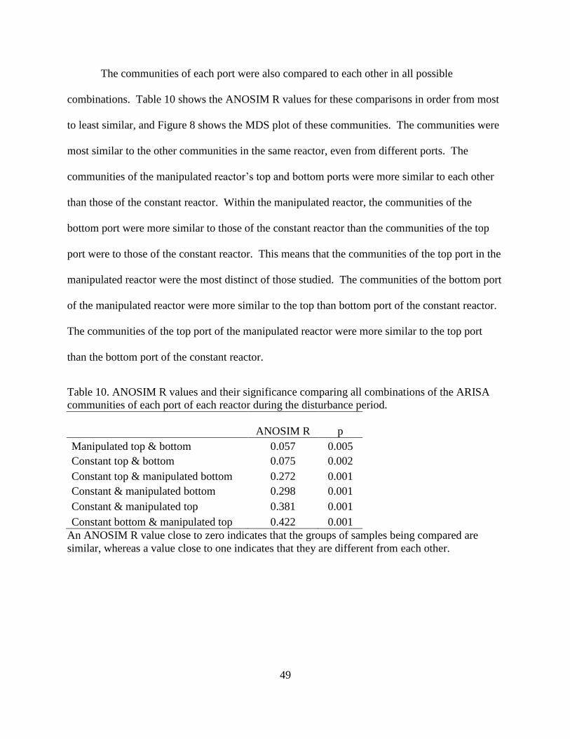
49
The communities of each port were also compared to each other in all possible
combinations. Table 10 shows the ANOSIM R values for these comparisons in order from most
to least similar, and Figure 8 shows the MDS plot of these communities. The communities were
most similar to the other communities in the same reactor, even from different ports. The
communities of the manipulated reactor’s top and bottom ports were more similar to each other
than those of the constant reactor. Within the manipulated reactor, the communities of the
bottom port were more similar to those of the constant reactor than the communities of the top
port were to those of the constant reactor. This means that the communities of the top port in the
manipulated reactor were the most distinct of those studied. The communities of the bottom port
of the manipulated reactor were more similar to the top than bottom port of the constant reactor.
The communities of the top port of the manipulated reactor were more similar to the top port
than the bottom port of the constant reactor.
Table 10. ANOSIM R values and their significance comparing all combinations of the ARISA
communities of each port of each reactor during the disturbance period.
ANOSIM R p
Manipulated top & bottom 0.057 0.005
Constant top & bottom 0.075 0.002
Constant top & manipulated bottom 0.272 0.001
Constant & manipulated bottom 0.298 0.001
Constant & manipulated top 0.381 0.001
Constant bottom & manipulated top 0.422 0.001
An ANOSIM R value close to zero indicates that the groups of samples being compared are
similar, whereas a value close to one indicates that they are different from each other.
50
Figure 8. MDS plot of ARISA communities from both ports of both reactors during the
disturbance period. Each point represents a sample with multiple OTUs present. These samples
were collected from April 16, 2012 through December 10, 2012. The samples are classified
according to the reactor and port of origin. This plot includes communities from periods of high
and low water levels.
4.3.2 Denitrifying microbial communities
The results of the denitrifying communities data included 800 unique restriction
fragments from digests with both restriction enzymes. Each sample contained between five and
468 OTUs, with a median of 36 fragments per sample, including both digests. There was a
median of 17 fragments from the reactions digested with AluI and for those digested with HhaI.
There was a maximum of 227 fragments per AluI digest and 241 fragments per HhaI digest. The
median number of OTUs was 34 for the manipulated reactor and 38 for the constant reactor.
Unlike with the total bacterial communities, the similarity of the denitrifying
communities between the two reactors did not change before and after the regular disturbance
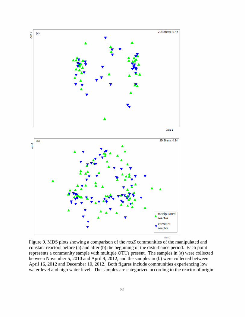
51
Figure 9. MDS plots showing a comparison of the nosZ communities of the manipulated and
constant reactors before (a) and after (b) the beginning of the disturbance period. Each point
represents a community sample with multiple OTUs present. The samples in (a) were collected
between November 5, 2010 and April 9, 2012, and the samples in (b) were collected between
April 16, 2012 and December 10, 2012. Both figures include communities experiencing low
water level and high water level. The samples are categorized according to the reactor of origin.
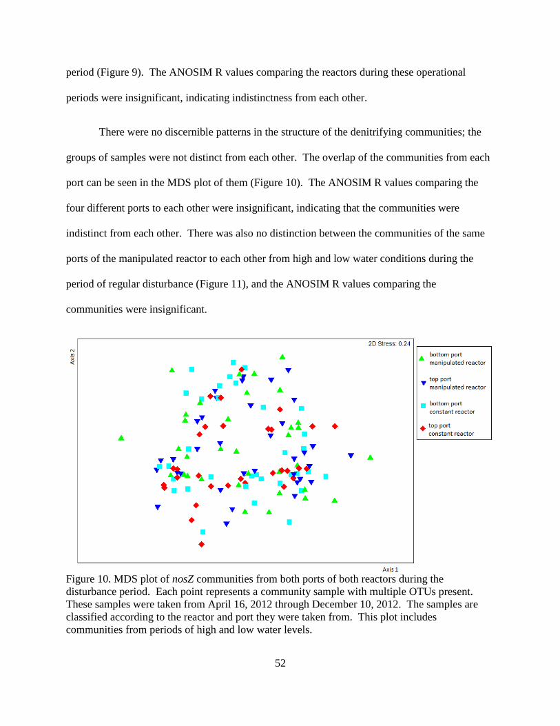
52
period (Figure 9). The ANOSIM R values comparing the reactors during these operational
periods were insignificant, indicating indistinctness from each other.
There were no discernible patterns in the structure of the denitrifying communities; the
groups of samples were not distinct from each other. The overlap of the communities from each
port can be seen in the MDS plot of them (Figure 10). The ANOSIM R values comparing the
four different ports to each other were insignificant, indicating that the communities were
indistinct from each other. There was also no distinction between the communities of the same
ports of the manipulated reactor to each other from high and low water conditions during the
period of regular disturbance (Figure 11), and the ANOSIM R values comparing the
communities were insignificant.
Figure 10. MDS plot of nosZ communities from both ports of both reactors during the
disturbance period. Each point represents a community sample with multiple OTUs present.
These samples were taken from April 16, 2012 through December 10, 2012. The samples are
classified according to the reactor and port they were taken from. This plot includes
communities from periods of high and low water levels.
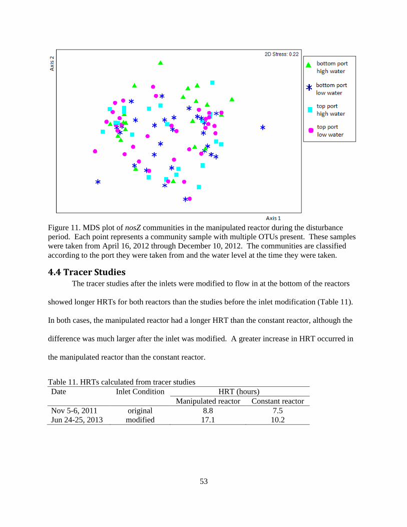
53
Figure 11. MDS plot of nosZ communities in the manipulated reactor during the disturbance
period. Each point represents a community sample with multiple OTUs present. These samples
were taken from April 16, 2012 through December 10, 2012. The communities are classified
according to the port they were taken from and the water level at the time they were taken.
4.4 Tracer Studies The tracer studies after the inlets were modified to flow in at the bottom of the reactors
showed longer HRTs for both reactors than the studies before the inlet modification (Table 11).
In both cases, the manipulated reactor had a longer HRT than the constant reactor, although the
difference was much larger after the inlet was modified. A greater increase in HRT occurred in
the manipulated reactor than the constant reactor.
Table 11. HRTs calculated from tracer studies
Date Inlet Condition HRT (hours)
Manipulated reactor Constant reactor
Nov 5-6, 2011 original 8.8 7.5
Jun 24-25, 2013 modified 17.1 10.2
54
4.5 Dissolved Oxygen Dissolved oxygen concentration in both ports of both reactors was measured twice, once
during a high water period and once during a low water period (Table 12). The dissolved oxygen
concentrations were less than 1 mg/L in the bottom port of the constant reactor. It was similarly
low in the bottom port of the manipulated reactor when the water level was high. When the
water level was low, the concentration in the bottom port was much closer to saturation (about 9
mg/L at room temperature). There was dissolved oxygen present in the top port of the constant
reactor, a few mg/L less than saturation, as well as in the top port of the manipulated reactor at
high water level.
Table 12. Dissolved oxygen concentration in each port. This was measured twice in fall 2012,
once at low water level and once at high water level.
Date Water level Dissolved Oxygen (mg/L)
Constant reactor Manipulated reactor
Top port Bottom port Top port Bottom port
9/28/2012 low 7.8 0.95 a 7.55
10/2/2012 high 6.92 0.59 5.02 0.95
a The concentration could not be measured in the top port of the manipulated reactor at low
water level, because it was not submerged.
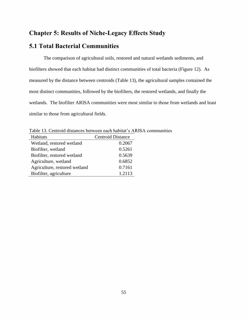
55
Chapter 5: Results of Niche-Legacy Effects Study
5.1 Total Bacterial Communities
The comparison of agricultural soils, restored and natural wetlands sediments, and
biofilters showed that each habitat had distinct communities of total bacteria (Figure 12). As
measured by the distance between centroids (Table 13), the agricultural samples contained the
most distinct communities, followed by the biofilters, the restored wetlands, and finally the
wetlands. The biofilter ARISA communities were most similar to those from wetlands and least
similar to those from agricultural fields.
Table 13. Centroid distances between each habitat’s ARISA communities
Habitats Centroid Distance
Wetland, restored wetland 0.2067
Biofilter, wetland 0.5261
Biofilter, restored wetland 0.5639
Agriculture, wetland 0.6852
Agriculture, restored wetland 0.7161
Biofilter, agriculture 1.2113
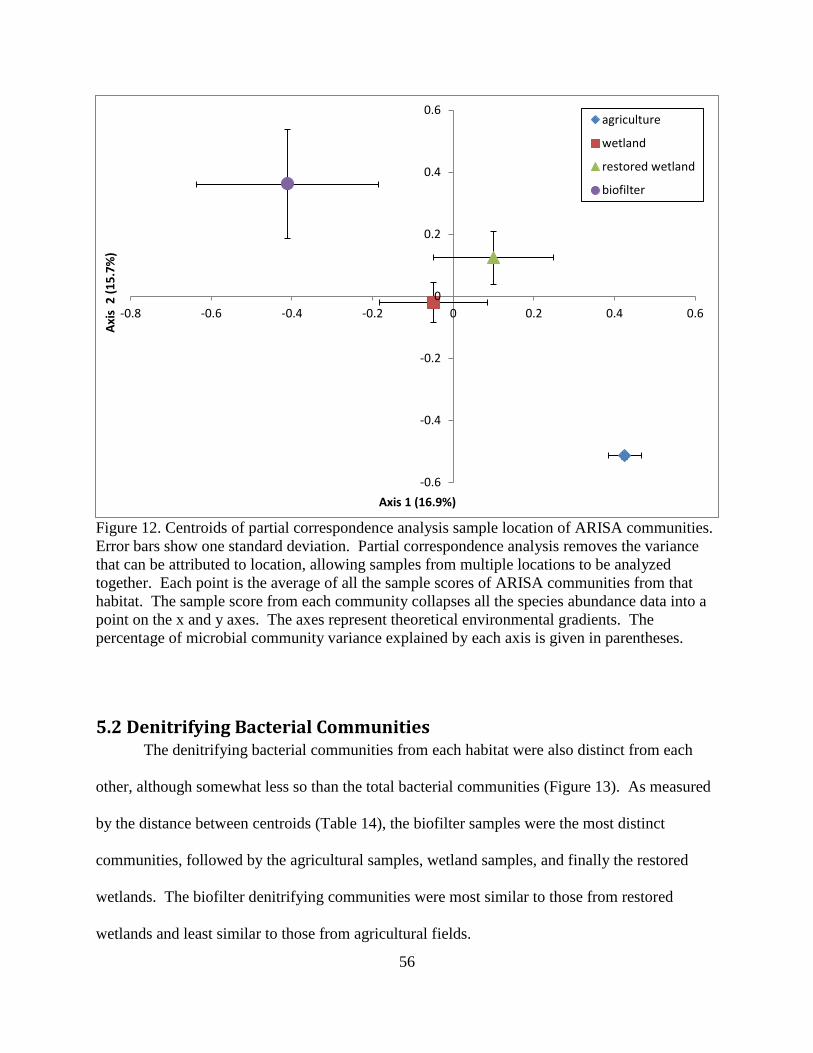
56
Figure 12. Centroids of partial correspondence analysis sample location of ARISA communities.
Error bars show one standard deviation. Partial correspondence analysis removes the variance
that can be attributed to location, allowing samples from multiple locations to be analyzed
together. Each point is the average of all the sample scores of ARISA communities from that
habitat. The sample score from each community collapses all the species abundance data into a
point on the x and y axes. The axes represent theoretical environmental gradients. The
percentage of microbial community variance explained by each axis is given in parentheses.
5.2 Denitrifying Bacterial Communities The denitrifying bacterial communities from each habitat were also distinct from each
other, although somewhat less so than the total bacterial communities (Figure 13). As measured
by the distance between centroids (Table 14), the biofilter samples were the most distinct
communities, followed by the agricultural samples, wetland samples, and finally the restored
wetlands. The biofilter denitrifying communities were most similar to those from restored
wetlands and least similar to those from agricultural fields.
-0.6
-0.4
-0.2
0
0.2
0.4
0.6
-0.8 -0.6 -0.4 -0.2 0 0.2 0.4 0.6
Axi
s 2
(1
5.7
%)
Axis 1 (16.9%)
agriculture
wetland
restored wetland
biofilter
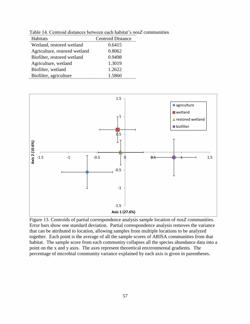
57
Table 14. Centroid distances between each habitat’s nosZ communities
Habitats Centroid Distance
Wetland, restored wetland 0.6415
Agriculture, restored wetland 0.8062
Biofilter, restored wetland 0.9498
Agriculture, wetland 1.3019
Biofilter, wetland 1.2622
Biofilter, agriculture 1.5860
Figure 13. Centroids of partial correspondence analysis sample location of nosZ communities.
Error bars show one standard deviation. Partial correspondence analysis removes the variance
that can be attributed to location, allowing samples from multiple locations to be analyzed
together. Each point is the average of all the sample scores of ARISA communities from that
habitat. The sample score from each community collapses all the species abundance data into a
point on the x and y axes. The axes represent theoretical environmental gradients. The
percentage of microbial community variance explained by each axis is given in parentheses.
-1.5
-1
-0.5
0
0.5
1
1.5
-1.5 -1 -0.5 0 0.5 1 1.5
Axi
s 2
(1
0.6
%)
Axis 1 (27.6%)
agriculture
wetland
restored wetland
biofilter
58
Chapter 6: Discussion
6.1 Laboratory Biofilters The three main components of the laboratory biofilter study are the performance of the
biofilters, the denitrification rates measured in the DEAs, and the microbial community structure,
total bacteria and denitrifying bacteria. The response of these to the water level disturbances will
be discussed, as will the relationships between performance, denitrification potential, and
microbial community structure.
The laboratory biofilters successfully removed 31% of the nitrate at high water level and
59% of the nitrate at low water level. For comparison to other biofilters, the total nitrate
removed per volume can be calculated given the influent nitrate loading and volume of the
inundated woodchip bed. The removal rates were 5 g N/day/m3 for both biofilters at high water
level and 9 g N/day/m3 for the manipulated biofilter at low water level. Therefore, the
performance of the laboratory biofilters falls within the range of 2-22 g N/day/m3 observed in the
literature (Schipper et al, 2010b).
The laboratory biofilters had better performance when the water level was low than when
it was high. This was different from the initial expectation that performance would be better at
high water level, because a greater portion of the reactor would be anoxic. Hypotheses tested to
explain this difference are that there was more dissolved oxygen at higher water level, short
circuiting was occurring at high water level, or that more carbon was available at low water
level. None of these were found to be conclusively true, although differences in carbon appear to
be the most likely cause of the performance difference.
59
One potential explanation is that more carbon could be released when the water level is
low. A greater portion of the reactor is aerobic, which could result in a faster carbon
mineralization rate of the woodchips (Moorman et al, 2010). To determine whether differences
in carbon availability were causing the difference in performance, DEAs with and without
glucose amendments were performed. If there were little to no difference between the amended
and unamended DEAs for the manipulated reactor but a difference between them for the constant
reactor, this would indicate that carbon was limiting denitrification at the high water level, but
not the low, causing the difference in performance. For both ports in both reactors, the nitrate
removal rates and nitrous oxide production rates were higher when measured with glucose
amendments than without, indicating that they are all carbon-limited. The difference in amended
and unamended nitrate removal rates was larger for the constant reactor than the manipulated
reactor. The smallest difference was between the DEAs for the top port of the manipulated
reactor, which, being close to the water level, would likely feel the strongest effect of increased
carbon. However, the differences in rates calculated from the two types of DEAs are not
different enough between the two reactors to conclude that carbon availability was the main
driver of performance differences.
Another possibility investigated is that differences in dissolved oxygen concentration in
the reactors caused the change in performance at high and low water level. If dissolved oxygen
were lower in the manipulated reactor at low water level than at high water level, this could
explain the difference in performance. As expected, the dissolved oxygen was highest in the
manipulated reactor when the water level was low, though, so dissolved oxygen concentrations
do not seem to be causing the different nitrate removal.

60
A third possible explanation for the improved performance at low water level is that there
are differences in actual HRT at different water levels, even though the theoretical HRT was the
same. If the HRT was much higher at the low water level than the high, this would explain the
differences in performance. The tracer studies performed by Bartolerio (2011) showed that the
HRT was 8.84 hours in the manipulated reactor at low water level and 7.52 hours in the constant
reactor. The HRT was longer at low water level than high, but only by 15%, whereas about
twice as much nitrate was removed at low water level than high. Therefore, the difference in
HRT does not fully explain the difference in performance. The similar construction of the two
reactors and their similar performance at the same water level also suggested that the constant
reactor and the manipulated reactor at high water level would have similar HRTs.
However, the change in performance after the inlet was modified suggests that
differences in the way water flows through the reactors are causing the changes. The inlet had
been modified so that the influent flowed in to the bottom of the reactor, rather than near the
water line. Following the modification, the nitrate removal by the constant reactor doubled,
whereas the removal in the manipulated reactor at low water level barely changed. The tracer
study after the inlet was modified showed an increase in the difference between the two reactors’
HRTs, which does not explain why the performance of the constant reactor became more similar
to the manipulated reactor. Furthermore, if the increase in performance in the constant reactor
were caused by a longer HRT, it seems likely that the even greater increase in the HRT of the
manipulated reactor would result in better performance, which was not the case.
One possible explanation for the performance improvement in the constant reactor after
modifying the inlet is that the bottom of the reactor, close to the inlet, could be an area of high
denitrification activity that started receiving more flow in the constant reactor once the inlet was
61
changed, thus increasing the overall nitrate removal. The flow would have been passing through
this part of the manipulated reactor at low water level anyway, which could be why the inlet
modification did not have a large effect on the manipulated reactor’s performance. The
denitrification potential was not measured at the bottom of the reactor, close to the inlet.
Another unexpected result in nitrate removal was the difference in performance in the
manipulated reactor right after weir removal and a week after weir removal. A potential
explanation is that it could be caused by differences in carbon degradation. Possibly, the optimal
conditions for carbon release from the woodchips occur in the portion of the reactor that was
previously inundated just after weir removal. Exposed to the air, oxygen was available for
aerobic respiration. This is supported by the faster degradation of woodchips near the top of
field biofilters, where there is more oxygen (Moorman et al, 2010). The woodchips were still
moist from the high water period, though.
DEAs were performed on woodchip samples from both ports of both biofilters to
compare the denitrification activity in different parts of the reactors and to determine which
operating conditions resulted in the highest denitrification rates. To my knowledge, all the DEAs
performed as part of other biofilter studies only measured nitrous oxide production, as is typical
for the assay, so only the nitrous oxide values in this study can be compared to the values found
in the literature. The range of values found for the laboratory biofilters in this study was
0.000015-0.004 mg N/hour/g woodchips for all DEAs and 0.00005-0.004 mg N/hour/g
woodchips when excluding the top port of the manipulated reactor during the extended dry
period, which had significantly lower denitrification potential than usual. In DEAs of woodchip
samples from a field biofilter, the denitrification rate ranged from 0.000176-0.00143 mg
N/hour/g woodchips (Moorman et al, 2010). Denitrification rates measured in DEAs of
62
woodchip samples from several lab reactors range from about 0.001-0.004 mg N/hour/g
woodchips (Warneke et al, 2011). The ranges of denitrification rates found in these two studies
are both within the range of the laboratory biofilters. This indicates that nitrous oxide production
rates observed in this work are reasonable for denitrifying biofilters. This study included many
more DEAs than either of the ones cited here, which may explain the wider range of values in
my work.
The denitrifying activity was very similar across reactors and across ports. Looking at
several different ways of classifying the disturbance conditions, this similarity persists. The
manipulated reactor was being disturbed by the changing water level, and indirectly the
environmental conditions that control denitrification were being changed. The microbes were
nevertheless able to maintain the same denitrification potential. Even with the changing
microbial communities, the denitrification potential was not that different, suggesting that these
communities were functionally redundant.
The exception to this similarity of denitrification potential is the top part of the disturbed
reactor, before regular disturbance. It was at low water level, and fairly dried out for an extended
period of time during this period, with moisture levels as low as 14% (data not shown). The
denitrification potential in this port was lower during this time than all the other groupings of
values. The water level does influence denitrification potential, but it takes a long time to see the
effect.
A surprising result observed from the DEAs was the discrepancy between nitrate removal
rates and the nitrous oxide production rates. If the nitrate is being removed by complete
denitrification and the rate is being accurately measured in the DEAs, these two rates should be
63
the same. However, the nitrate removal rates were ten times higher than the nitrous oxide
production rates.
The difference between nitrous oxide production and nitrate removal in DEAs is likely
due to incomplete blocking by acetylene. Alternative explanations are nitrous oxide dissolved in
the water, another method of nitrate removal besides denitrification, or incomplete
denitrification. Nitrous oxide has a Henry’s Law constant of 0.025 mol/kg/bar (NIST), which is
0.62 when converted to be dimensionless. The equilibrium concentration in water is less than in
air, and the bottles in which the assays were performed were shaken prior to sampling to release
dissolved gas. Nitrous oxide dissolved in the water would therefore not cause a ten-fold decrease
in the measurement.
Another potential explanation for the discrepancy is that nitrate is being removed from
the solution by methods other than denitrification. Nitrate can be used for cell growth. Given
that the addition of chloramphenicol prevents new protein synthesis, it seems unlikely that this
much nitrate would be removed via cell growth. Nitrate could also be removed via the
Anammox process, in which nitrite is the electron acceptor for ammonia oxidation (Mulder et al,
1995). No ammonia is added to the solution in the DEAs, so it seems unlikely that sufficient
ammonia is present for ten times more nitrate to be removed via Anammox than denitrification.
Incomplete denitrification is another potential explanation for the discrepancy between
nitrous oxide production and nitrate removal measured in the DEAs. Possibly nitrate is being
reduced, but is not being converted all the way to nitrous oxide. This would have potential
implications for biofilter implementation, because if nitrate is not being transformed all the way
to N2, one environmental quality problem is being traded for another. No nitrite has been
64
detected in the water samples collected during DEAs, so denitrification is occurring at least past
the reduction of nitrite. Nitric oxide has not been measured in the gas samples, so it is possible
that this is the limiting step where denitrification is not going to completion. This leaves
incomplete blocking of nitrous oxide reduction by acetylene and incomplete denitrification as the
two likely causes of the discrepancy. If incomplete blocking is the cause, the nitrate removal
rates are a better measurement of denitrification potential than the nitrous oxide production rates,
but if incomplete denitrification is the cause, nitrous oxide production rates are the better
measurement.
The total bacterial and denitrifying bacterial communities in the laboratory biofilters were
investigated to determine the effects of the changing water level on them. Also, the differences
in the diversity and community structure between the two reactors and between the top and
bottom (constantly inundated) ports were compared.
The regular disturbance of the reactors resulted in the development of total bacterial
communities distinct from the communities of the constant reactor. However, the communities
of the manipulated reactor at low water level were not significantly different from those at high
water level. This suggests that specific disturbance communities are being formed, rather than
high water level communities and low water level communities.
Increased disturbance severity caused the greatest dissimilarity to other communities.
This is evident from the ANOSIM R values comparing the top port of the disturbed reactor
during regular disturbance to other ports at the same time. The top port was the most severely
disturbed port in the reactor, because it was inundated at high water level, but just at the water
level when the weir was removed. The bottom port, though, was inundated at all times, even
65
with the changing water level. Both ports of the constant reactor were more similar to the
bottom port of the manipulated reactor than the more severely disturbed top port, indicating that
the more severe disturbance was associated with a more distinct bacterial community.
The denitrifying bacterial communities, though, appear to be less affected by the
changing water level than the total bacterial communities. No significant differences were
observed between the communities of each reactor or between the communities of the
manipulated reactor at high and low water level. This suggests that the denitrifying communities
are resistant to disturbance by changing water level. This resistance may be because most
denitrifying bacteria are facultative anaerobes (Zumft, 1997) and would be successful in a habitat
with increased oxygen. Although moisture and carbon were also likely changing in the
manipulated reactor with the varying water level, the denitrifying bacteria do not appear to have
been sensitive to the change in these conditions.
6.2 Niche-legacy Study In the comparison of microbial communities from different habitats, microbial
communities in the biofilters were completely distinct from the communities found in
agricultural soil and natural and restored wetland sediment. This suggests that the communities
of the biofilters have developed primarily based on the influence of the environmental conditions
there. The biofilter communities were even more dissimilar to those from agricultural soil than
the wetland communities were from the agricultural soil. There was not an observable effect of
the legacy of historical agricultural land use on the biofilter microbial communities. This was
true for both the total bacterial communities and the denitrifying bacterial communities.
66
The literature review showed both niche and legacy having an effect on the microbial
community structure. Of the papers included in the literature review of this thesis, both of the
studies comparing habitats with different current land use primarily showed niche effects ( Jesus
et al, 2009, Waldrop et al, 2010). The habitat comparison in this thesis is most similar in concept
to the experimental design of these disturbed/undisturbed habitat comparison studies, so it makes
sense that the biofilter habitat comparison would have results similar to these studies. Like
Peralta et al (2010), a difference in the microbial community structure of natural and restored
wetlands was also observed in this habitat comparison. Looking at the larger scale, though, in
which habitats are more environmentally different, shows a stronger niche effect on microbial
community composition.
The results of this habitat comparison indicate that microbial communities can
successfully be encouraged to develop through the implementation of the right environmental
conditions. Many engineered ecosystems depend on microbes to degrade contaminants, as in the
case of the denitrifying biofilters. This further validates the importance of studying microbial
communities in engineered ecosystems and the ecological drivers that influence their
composition.
67
Chapter 7: Conclusions
The laboratory biofilter study was conducted to observe the performance, denitrification
activity, and microbial communities under constant conditions and under changing water level
conditions. Active field biofilters experience variable flow and thus variable HRT, so the
changing water level should give insight into the effects of this flow variability on denitrification
within the reactors and the microbes responsible for carrying it out.
The performance of the laboratory biofilters was sensitive to the effects of changing
water level, even with a constant HRT. About twice as much nitrate was removed at low water
level than high. This difference is likely due to changes in flow patterns within the biofilters at
different water levels. Based on the evidence of the DEAs with and without glucose, the lower
water level also seems to increase the release of carbon from the woodchips, increasing the
nitrate removal in the reactors. This suggests that the water depth of the biofilters should be
considered in design to optimize nitrate removal.
The denitrification activity was similar in both reactors under almost all conditions. The
only time water level appeared to influence the denitrification activity was in the top port during
the period of long-term low water level, when these woodchips became dried out. This indicates
that denitrification should not decrease due to short-term decreases in flow through the biofilter.
The bacterial communities from the two reactors became more divergent from each other
after the period of regular disturbance began. Distinct disturbance communities appeared to
develop, rather than high or low water level communities, with the most severely disturbed parts
of the biofilter having the most different microbial communities. The changing bacterial
communities did not affect denitrification.

68
The denitrifying bacterial communities were not different from each other between the
different reactors, ports, or disturbance conditions. In spite of the changing water level, these
communities exhibited a high level of resistance.
One of the original hypotheses that motivated the laboratory biofilter study was that the
changing water level would encourage the development of microbial communities able to rapidly
recover after disturbance. Functional redundancy was observed in the total bacterial
communities with respect to denitrification and denitrifying bacterial communities were
unaffected by the changing water level. Although the water level had a strong effect on the
performance of the denitrifying biofilters, it seems to be primarily due to the environmental
conditions in the reactors, rather than due to the microbial community composition.
The results of the niche-legacy comparison showed differentiation of the microbial
communities of each habitat. Both the total and denitrifying bacterial communities in the field
biofilters were independent of their source community, agricultural soil, and those from a
somewhat similar environment, wetlands. This suggests that environmental conditions can be
used to encourage the development of particular microbial communities in engineered
ecosystems.
Some future work is recommended to further elucidate the effects of changing water level
on the biofilters. To gain a better understanding of the effect of changing water level on
performance, a shorter term study of the nitrate removal of the biofilters should be conducted.
The inlet should be set up as it was after the modification, in which the water enters the biofilter
at the bottom. This will test whether water level affects the performance of the reactor and how,
when the inlet is not causing the differences. A study of the same length as the one already
69
performed is unnecessary, because a few months will be sufficient to observe the performance
for several weeks at each water level. Although the results of the tracer studies did not show a
shorter residence time in the reactors at high water level, the performance was the same in the
two reactors at different water levels once the inlet was changed. This additional study will
clarify the effect of water level, independent of changes it may have caused in flow through the
reactor.
Second, to more completely study the effect of disturbance on the microbial
communities, the biofilters should be pushed to failure. How long does it take for denitrification
potential to return to its previous level? Does the microbial community structure return to its
pre-disturbance state, and if so, how long does that rebound take? A more severe disturbance
should be imposed that results in drastically less nitrate removal and a large change in microbial
community composition. Some potential disturbances that are experienced by field biofilters
include changes in influent flow rate, nitrate loading, or HRT. Injection of a pesticide is another
potential way to realistically disturb the laboratory biofilters. This second proposed experiment
would also be useful for reliability modeling of the denitrifying biofilters, continuing the work of
Nick Bartolerio (2011).
Thirdly, the cause of the discrepancy between nitrate removal and nitrous oxide
production should be further investigated. To do this, the gas samples collected during the DEAs
should be analyzed for nitric oxide. If it accumulated over time during the assays, this indicates
that nitric oxide reduction is the rate-limiting step of denitrification for the biofilter microbes. If
this is the case, the nitrous oxide production rates are the better measure of denitrification
potential. If the possibility of nitric oxide accumulation is eliminated, this leaves incomplete
70
blocking by acetylene of nitrous oxide reduction as the likely explanation. If this is the case, the
nitrate removal rates are the better measure of denitrification potential in the biofilters.
Overall, the performance of the reactor is sensitive to the operating conditions, and the
bacterial communities changed in response to the changing water level. However, the
denitrification potential was not as sensitive, and the denitrifying bacterial communities within
the reactors displayed resistance under the water level disturbance. The microbial communities
of the biofilters were distinct from the communities in agricultural soil or natural or restored
wetland sediments.
These results have positive implications for the removal of nitrate from agricultural
runoff before it reaches sensitive water bodies through good performance by denitrifying
biofilters. The functional redundancy of the total bacteria and resistance of the denitrifying
bacteria under water level disturbance indicate that the microbes in the field biofilters should be
able to successfully carry out denitrification, even when subjected to variable flow rate. The
sensitivity of the biofilter performance to changing water level, though, suggests that nitrate
removal in the reactors is highly dependent on either the HRT or other conditions. This can be
addressed in the design of the biofilters to maximize nitrate removal. The niche-legacy habitat
comparison also shows a strong effect of environmental conditions rather than legacy effects on
the microbial community composition of the biofilters. This is encouraging in that
environmental conditions can be used to develop microbial communities effective at nitrate
removal.
71
References
Andrus, J.M. (2011) Microbial Community Analysis for denitrifying biofilters. PhD dissertation,
University of Illinois at Urbana-Champaign, Urbana, IL.
Ayarza, J., Erijman, L. (2011) Balance of neutral and deterministic components in the dynamics
of activated sludge floc assembly. Environmental Microbiology. 61: 486-495
Bartolerio, N.A. (2011) Development and application of a microbial reliability model to analyze
denitrifying biofilter stability. M.S. thesis, University of Illinois at Urbana-Champaign, Urbana,
IL.
Baxter, A.M., Johnson, L., Edgerton, J., Royer, T., Leff, L.G. (2012) Structure and function of
denitrifying bacterial assemblages in low-order Indiana streams. Freshwater Science 31: 304-
317.
Blowes, D.W., Robertson, W.D., Ptacek, C.J., Merkley, C. (1994) Removal of agricultural nitrate
from tile-drainage effluent water using in-line bioreactors. Journal of Contaminant Hydrology
15: 207-221.
Boyle, S.A., Rich, J.J., Bottomley, P.J., Cromack, J.K., Myrold, D.D. (2006) Reciprocal transfer
effects on denitrifying community composition and activity at forest and meadow sites in the
Cascade Mountains of Oregon. Soil Biology and Biochemistry 38: 870-878.
Cameron, S.G., Schipper, L.A. (2010) Nitrate removal and hydraulic performance of carbon
substrates for potential use in denitrification beds. Ecological Engineering 36: 1588-1595.
Carleton, J.N., Grizzard, T.J., Godreh, A.N., Post, H.E. (2001) Factors affecting the performance
of stormwater treatment wetlands. Water Research 35: 1552-1562.
Cavigelli, M.A., Robertson, G.P. (2000) The functional significance of denitrifier community
composition in a terrestrial ecosystem. Ecology 81: 1402-1414.
Christianson, L.E., Helmers, M.J., Bhandari, A. (2010) Bioreactor design geometry effects on
nitrate removal. ASABE Paper #IDS-CSBE100073.
Christianson, L.E., Bhandari, A., Helmers, M.J. (2011) Pilot-scale evaluation of denitrification
drainage bioreactors: reactor geometry and performance. Journal of Environmental Engineering
137: 213-220.
Clarke, K.R. and Green, R.H. (1988) Statistical design and analysis for a" biological effects"
study. Marine Ecology Progress Series 46: 213-226.
Cooke, R.A., Doheny, A.M., Hirschi, M.C. (2001) Bio-reactors for edge-of-field treatment of tile
outflow. ASABE Paper #0120181-17.
72
Cuddington, K. (2011) Legacy effects: The persistent impact of ecological interactions.
Biological Theory 6: 203-210.
David, M. B., Drinkwater, L. E,; McIsaac, G. F. (2010) Sources of nitrate yields in the
Mississippi River Basin. Journal of Environmental Quality 39: 1657-1667.
Doheny, A.M. (2003) Amelioration of tile nitrate-N and atrazine using inline biofilters. M.S.
thesis, University of Illinois at Urbana-Champaign, Urbana, IL.
Fisher, M.M., and Triplett, E.W. (1999) Automated approach for ribosomal intergenic spacer
analysis of microbial diversity and its application to freshwater bacterial communities. Applied
and Environmental Microbiology 65: 4630-4636.
Forster, P., Ramaswamy, V., Artaxo, P., Berntsen, T., Betts, R., Fahey, D.W., Haywood, J.,
Lean, J., Lowe, D.C., Myhre, G., Nganga, J., Prinn, R., Raga, G., Schulz, M., Van Dorland, R.
(2007) Changes in Atmospheric Constituents and in Radiative Forcing. In: Climate Change
2007: The Physical Science Basis. Contribution of Working Group I to the Fourth Assessment
Report of the Intergovernmental Panel on Climate Change [Solomon, S., D. Qin, M. Manning, Z.
Chen, M. Marquis, K.B. Averyt, M.Tignor and H.L. Miller (eds.)]. Cambridge University Press,
Cambridge, United Kingdom and New York, NY, USA.
Fraterrigo, J., Balser, T., Turner, M. (2006) Microbial community variation and its relationship
with nitrogen mineralization in historically altered forests. Ecology 87: 570-579.
Gopalakrishnan, G., Negri, M.C., Salas, W. (2012) Modeling biogeochemical impacts of
bioenergy buffers with perennial grasses for a row-crop field in Illinois. Global Change Biology
Bioenergy 4: 739-750.
Griffiths, B.S., Hallett, P.D., Kuan, H.L., Gregory, A.S., Watt, C.W., Whitmore, A.P. (2008)
Functional resilience of soil microbial communities depends on both soil structure and microbial
community composition. Biology and Fertility of Soils 44: 745–754.
Groffman, P.M., Gold, A.J., Addy, K. (2000) Nitrous oxide production in riparian zones and its
importance to national emission inventories. Chemosphere – Global Change Science 2: 291-299.
Gibert, O., Pomierny, S., Rowe, I., Kalin, R.M. (2008) Selection of organic substrates as
potential reactive materials for use in a denitrification permeable reactive barrier wall (PRB).
Bioresource Technology 99: 7587-7596.
Greenan, C.M., Moorman, T.B., Kaspar, T.C., Parkin, T.B., Jaynes, D.B. (2006) Comparing
carbon substrates for denitrification of subsurface drainage water. Journal of Environmental
Quality 35: 824-829.
73
Greenan, C.M., Moorman, T.B., Parkin, T.B., Kaspar, T.C., Jaynes, D.B. (2009) Denitrification
in wood chip bioreactors at different water flows. Journal of Environmental Quality 38: 1664-
1671.
Holtan-Hartwig, L., Dorsch, P., Bakken, L.R. (2000) Comparison of denitrifying communities in
organic soils: kinetics of NO3- and N2O reduction. Soil Biology and Biogeochemistry 32:833-
843.
Howarth, R.W., Marino, R. (2006) Nitrogen as the limiting nutrient for coastal marine
ecosystems: Evolving views over three decades. Limnology and Oceanography 51: 364-376.
Hutchinson, G.E. (1957) Concluding remarks. Cold Spring Harbor Symposium 22:415–427.
Jaynes, D.B., Kaspar, T.C., Moorman, T.B., Parkin, T.B. (2008) In situ bioreactors and deep-
pipe drain-pipe installation to reduce nitrate losses in artificially drained fields. Journal of
Environmental Quality 37: 429–436.
Jesus, E., Marsh, T., Tiedje, J., Moreira, F. (2009) Changes in land use alter the structure of
bacterial communities in Western Amazon soils. The ISME Journal. 3:1004-1011.
Kalita, P.K., Algoazany, A.S., Mitchell, J.K., Cooke, R.A., and Hirschi, M.C. (2006) Subsurface
water quality from a flat tile-drained watershed in Illinois, USA. Agriculture, Ecosystems &
Environment 115: 183-193.
Kulmatiski, A., Beard, K. (2008) Decoupling plant-growth from land use legacies in soil
microbial communities. Soil Biology and Biogeochemistry 40: 1059-1068.
Langenheder, S., Lindström, E. Tranvik, L. (2005) Weak coupling between community
composition and functioning of aquatic bacteria. Limnology and Oceonography. 50: 957-967.
Langenheder, S., Lindström, E. Tranvik L. (2006) Structure and function of bacterial
communities emerging from different sources under identical conditions. Applied and
Environmental Microbiology 72: 212-220.
Long, L.M., Schipper, L.A., Bruesewitz, D.A. (2011) Long-term nitrate removal in a
denitrification wall. Agriculture, Ecosystems & Environment 140: 514-520.
Ma, W.K., Bedard-Haughn, A., Siciliano, S.D., Farrell, R.E. (2008) Relationship between
nitrifier and denitrifier community composition and abundance in predicting nitrous oxide
emissions from ephemeral wetland soils. Soil Biology and Biogeochemistry 40:1114-1123.
Moorman, T.B., Parkin, T.B., Kaspar, T.C., Jaynes, D.B. (2010) Denitrification activity, wood
loss, and N2O emissions over 9 years from a wood chip bioreactor. Ecological Engineering 36:
1567-1574.
74
Mulder, A., van de Graaf, A.A., Robertson, L.A., Kuenen, J.G. (1995) Anaerobic ammonium
oxidation discovered in a denitrifying fluidized bed reactor. FEMS Microbiology Ecology 16:
177-183.
Osborne, L.L. and Kovacic, D.A. (1993) Riparian vegetated buffer strips in water-quality
restoration and stream management. Freshwater Biology 29: 243-258.
Peralta, A., Matthews, J., Kent, A. (2010) Microbial community structure and denitrification in a
wetland mitigation bank. Applied and Environmental Microbiology 76: 4207-4215.
Philippot, L. (2002) Denitrifying genes in bacterial and Archaeal genomes. Biochimica et
Biophysica Acta 1577: 355-376.
Porter, M.D. (2011) Microbial community dynamics in denitrifying biofilters receiving
agricultural drainage. M.S. thesis, University of Illinois at Urbana-Champaign, Urbana, IL.
Rawls, J.F., Mahowald, M.A., Ley, R.E., Gordon, J.I. (2006) Reciprocal gut microbiota
transplants from zebrafish and mice to germ-free recipients reveal host habitat selection. Cell
127: 423-433.
Rich, J.J., Heichen, R.S., Bottomley, P.J., Cromack, J.K., Myrold, D.D. (2003) Community
composition and functioning of denitrifying bacteria from adjacent meadow and forest soils.
Applied and Environmental Microbiology 69: 5974-5982.
Rich, J.J., Myrold, D.D. (2004) Community composition and activities of denitrifying bacteria
from adjacent agricultural soil, riparian soil, and creek sediment in Oregon, USA. Soil Biology
and Biochemistry 36: 1431-1441.
Robertson, W.D., Cherry, J.A. (1995) In situ denitrification of septic-system nitrate using
reactive porous media barriers: field trials. Ground Water 33: 99–111.
Robertson, W.D., Vogan, J.L., Lombardo, P.S. (2008) Nitrate removal rates in a 15-year-old
permeable reactive barrier treating septic system nitrate. Groundwater Monitoring &
Remediation 28: 65-72.
Sambrook, J., and D. Russell (2001) Molecular cloning: a laboratory manual. Cold Spring
Harbor, NY: Cold Spring Harbor Laboratory Press.
Sanford, R.A., Wagner, D.D., Wu, Q., Chee-Sanford, J.C., Thomas, S.H., Cruz-García, C.,
Rodríguez, G., Massol-Deyáe, A., Krishnani, K.K., Ritalahti, K.M., Nissen, S., Konstantinidis,
K.T., Löffler, F.E. (2012) Unexpected nondenitrifier nitrous oxide reductase gene diversity and
abundance in soils. Proceedings of the National Academy of Science 109: 19709-19714.
75
Schipper, L.A., Cameron, S.C., Warneke, S. (2010a) Nitrate removal from three different
effluents using large-scale denitrification beds. Ecological Engineering 36: 1552-1557.
Schipper, L.A., Robertson, W.D., Gold, A.J., Jaynes, D.B., Cameron, S.C. (2010b) Denitrifying
bioreactors – An approach for reducing nitrate loads to receiving waters. Ecological Engineering
36: 1532-1543.
Schipper, L., Vojvodic-Vukovic, M. (1998) Nitrate removal from ground water using a
denitrification wall amended with sawdust: field trial. Journal of Environmental Quality 27:
664–668.
Soares, M.I.M., Abehovich, A. (1998) Wheat straw as substrate for water denitrification. Water
Research 32: 3790-3794.
Stone, M. and Krishnappan, B. (1997) Transport characteristics of tile-drain sediments from an
agricultural watershed. Water Air & Soil Pollution 99: 89-103.
Strickland, M., Lauber, C., Fierer, N. & Bradford, M. (2009) Testing the functional significance
of microbial community composition. Ecology 90: 441-451.
Tanner, R.S. (1997) “Cultivation of bacteria and fungi” in Manual of Environmental
Microbiology, C.J. Hurst, G.R. Knudsen, M.J. McInerney, L.D. Stetzenbach, and M.V. Walter,
eds., American Society for Microbiology, Washington, D.C., 52-60.
ter Braak, C. J. F, and P. Smilauer (ed.). 2002. CANOCO reference manual and CanoDraw for
Windows user's guide: software for canonical community ordination (version 4.5). Wageningen
University and Research Center Publications, Wageningen, Netherlands.
Tiedje, J.M., Simkins, S., Groffman, P.M. (1989) Perspectives on measurement of denitrification
in the field including recommended protocols for acetylene based methods. Plant and Soil 115:
261-284.
van Driel, P.W., Robertson, W.D., Merkley, L.C. (2006) Denitrification of agricultural drainage
using wood-based reactors. Transactions of the ASABE 49: 565-573.
Volokita, M., Abehovich, A., Soares, M.I.M. (1996) Denitrification of groundwater using cotton
as energy source. Water Science and Technology 34: 379-385
Waldrop, M., Balser, T., Firestone, M. (2000) Linking microbial community composition to
function in a tropical soil. Soil Biology and Biogeochemistry 32: 1837-1846.
Wallenstein, M.D., Myrold, D.D., Firestone, M., Voytek, M. (2006) Environmental controls on
denitrifying communities and denitrification rates: insights from molecular methods. Ecological
Applications 16: 2143-2152.
76
Warneke, S., Schipper, L.A., Matiasek, M.G., Scow, K.M., Cameron, S., Bruesewitz, D.A.,
McDonald, I.R. (2011) Nitrate removal, communities of denitrifiers and adverse effects in
different carbon substrates for use in denitrification beds. Water Research 45: 5463-5475.
Wildman, T.A. (2002) Design of field-scale bioreactors for bioremediation of nitrate-N in tile
drainage effluent. M.S. thesis, University of Illinois at Urbana-Champaign, Urbana, IL.
Woli, K.P., David, M.B., Cooke, R.A., McIsaac, G.F., Mitchell, C.A. (2010) Nitrogen balance in
and export from agricultural fields associated with controlled drainage systems and denitrifying
bioreactors. Ecological Engineering 36: 1558–1566.
Zumft, W.G. (1997) Cell biology and molecular basis of denitrification. Microbiology and
Molecular Biology Reviews 61: 533-616.

77
Appendix
A.1 Laboratory Procedures
A.1.1 Biofilter Woodchip Sampling Procedure for Microbial Community Analysis Adapted from Matthew Porter’s procedure for field biofilter sampling.
Prior to Sampling
1. Wash and autoclave one 250 mL Nalgene sampling bottle for each port.
2. Weigh each sampling bottle without the lid and write the weight on the bottle.
3. Prepare Ringer’s solution by adding 250 mL of nanopure water to 2 Ringer’s tablets (Oxoid Limited, UK) and autoclaving on a 30 liquid cycle.
4. Autoclave a 250 mL graduated cylinder, 5 mm glass beads, and 1.5 mL centrifuge tubes
on a 30 gravity cycle.
Sample Collection
1. Sterilize tweezers by covering in 70% ethanol and flaming.
2. Add at least 15 g woodchips from the bottom of the port to the appropriate sampling
bottle.
Sample Processing
1. Remove woodchips from each bottle until 15 g remain.
2. Add 110 mL of sterile Ringer's solution to each bottle using a sterile graduated cylinder.
3. Place the bottles on the shaker tray in the 30ºC room overnight.
4. Label 1.5 mL centrifuge tubes with the date, reactor, and port. Label three tubes for each
port.
5. Remove the bottles from the warm room to work at the lab bench.
6. Vigorously shake the bottles with the woodchip wash (the Ringer's solution in which the
woodchips have been shaken), and transfer as much of the liquid as will fit into sterile,
appropriately marked 50 mL centrifuge tubes.
7. Spin down the woodchip wash for 3 minutes at 5000xg.
8. Pour off the supernatant into a waste beaker.
9. Repeat steps 6-8, adding the woodchip wash to the same centrifuge tubes as before, until
all the woodchip wash has been used. This should take two to three spins.
10. Add 2.5 mL of 1X PBS and 5 sterile glass beads to each 50 mL centrifuge tube.
11. Vortex each 50 mL centrifuge tube for 2 minutes on the high setting.
12. After vortexing, centrifuge at 750xg for 5 minutes.
13. Pipet 1 mL of the supernatant into each of the sterile, labeled 1.5 mL centrifuge tubes
using sterile large orifice pipette tips. There should be two to three 1.5 mL centrifuge
tubes for each port.
14. Store the DNA sample tubes at -20ºC until extraction.

78
A.1.2 DNA Extraction Protocol Modified from the manufacturers’ instructions by J. Malia Andrus to increase DNA yields. This
uses the FastDNA Spin Kit (MP Biomedicals, Solon, OH).
1. Before beginning, load five 2 mL mid-sci tubes with autoclaved nanopure H2O. Place
these tubes into the block heater. Set the heater on low and at the 65C mark. The water
will be needed in the washing step.
2. Use a 96-tube plate, and set up the following tubes in this order vertically:
a. One lysis tube per sample (in soil spin kit)
b. One 1.5 mL tube per sample (on bench top)
c. One Spin Module per sample (in soil spin kit)
d. One 1.5 mL tube per sample (on bench top)
3. Label the tops of each of the tubes with sample name and date.
4. Vortex each sample, and add 400 L of the sample to its lysis tube.
5. Add 1 mL of CLS-TC to each lysis tube.
6. Load the lysis tubes in the Fast Prep Machine. Ensure that the machine is balanced and
the spindle is securing each tube in place. Run for 40 seconds at 5 m/s.
7. Centrifuge the lysis tubes for 5 mins at max speed.
8. Pipette 700 L of supernatant into each sample’s respective 2 mL tube.
9. Add 700 L (equivalent to the volume of DNA) of binding matrix, into each 2 mL tube.
10. Transfer all of the 1.5 mL tubes into a 96 well tray, place the lid on the tray and slowly
turn the tray up and down for 5 mins.
11. After 5 mins are up, centrifuge the 1.5 mL tubes for 1 min at max speed.
12. Pipette about half of the liquid out (700 L) into a waste liquid container, but make sure
to leave some liquid near the top of the glass bead level.
13. Re-suspend the glass beads with the remaining liquid, and pipette into the basket tube.
14. Spin the basket tubes for 1 min at max speed, to separate the liquid from the beads.
15. Empty the liquid from the basket tube into the waste liquid container.
16. Pipette the remaining extraction liquid into the now empty 1.5 mL tube (should get about
500 L).
17. Add an equivalent volume of binding matrix into each of the tubes.
18. Repeat steps 10 through 15.
19. Add 500 L of SEWS to the basket tube and centrifuge for 1 min.
20. Empty the wash into the waste container.
21. Add another 500 L of SEWS to the basket tube and centrifuge again for 1 min.
22. Empty the wash into the waste container.
23. Centrifuge for 1 min to remove any remaining ethanol.
24. Place the basket into the remaining 1.5 mL tube.
25. Add 100 L of 65C water to the glass beads in the basket.
26. Vortex the samples, and then centrifuge for 1 min (The tops will pop open, so place the
tubes into the centrifuge so that the lid opens down.
27. Store at -20oC until further analysis.
79
A.1.3 CTAB Cleanup Procedure Established CTAB procedure of Angela Kent’s laboratory.
working CTAB stock recipe (10% CTAB/0.7 M NaCl):
1. Dissolve 4.1 g NaCl in 80 mL H2O.
2. Place on heater/stirrer with stirring bar.
3. Slowly add 10 g CTAB (cetyl trimethyl ammonium bromide)
4. Adjust final volume to 100 mL.
5. Autoclave.
Purification protocol
1. Pre-warm working CTAB stock to 65C in a 1.5 mL tube in the heat block.
2. Transfer 100 mL of the extracted DNA into a 1.5 mL tube for each sample.
3. Label (long-term storage) one autoclaved 1.5 mL tube for each DNA extraction.
4. Add 16.25 mL of 5 M NaCl (autoclaved) to each DNA extract to adjust the NaCl
concentration of each DNA extract to 0.7 M.
5. Add 12 mL of warm working CTAB stock (0.1 vol). Mix thoroughly and incubate at
65C for 15 mins. *use filter tips
6. Add 128 mL (one volume) of chloroform:isoamyl alcohol (24:1). Mix carefully but
thoroughly. Centrifuge at maximum speed (14,000 x g) for 5 mins.
*Use filter tips; do not collect white interface layer (only transfer top layer for
precipitation)
7. Carefully remove the top layer to a clean, well-labeled 1.5 mL tube (should get about 125
mL). Add 256 mL (two volumes) of cold 100% EtOH to precipitate the DNA. After
adding/mixing 100% EtOH, increase precipitation of DNA by putting samples in the
freezer (-20C) overnight.
8. Mix thoroughly and centrifuge at maximum speed for 15 mins (increase time to increase
expected yield).
***Make sure to orient the tubes in the same direction (e.g. hinge side point out) so you
know the location of the DNA (if hinge side facing out, DNA will be along the side of the
hinge).
9. Carefully avoiding the pellet, remove supernatant. Add 125 mL 70% EtOH (cold), flick
to mix, and centrifuge at maximum speed for 7 mins.
10. Repeat step 9 once.
11. Remove supernatant. Allow pellet to air dry (approximately 15 mins – this may take
longer and be careful not to dry down samples all the way). Place tubes upside-down,
propped against a tube rack and over kim wipes.
12. Resuspend pellet in 50 mL dH2O.
13. Wash back side of tube (where DNA is supposed to be) with dH2O using the pipet. If you
orient all your tubes hinge side out in the centrifuge, then the DNA should be along the
hinge side, so make sure you run water down that side.
14. Store at -20C until further analysis.
80
A.1.4 Denitrification Enzyme Assay Protocol Adapted from Nicholas Bartolerio’s DEA procedure, based on the acetylene block method
described by Tiedje et al. (1989).
1. Mix a solution of 15 mg/L NO3- and 0.1 g/L chloramphenicol in nanopure water.
2. Measure solution into 75 mL aliquots for each DEA to be carried out. Aliquots should be
stored in autoclaved 125 mL Nalgene sampling bottles.
3. Sample woodchips from each port using sterile tweezers, as for the microbial community
sampling.
4. Add 10 g of woodchips into a labeled 150 mL Wheaton bottle. Duplicate assays should
be performed for each port. Record the mass of the bottle empty and with woodchips.
5. Pour nitrate-chloramphenicol solution into each Wheaton bottle.
6. Close the Wheaton bottles with lids fitted with rubber septa.
7. Flush the bottle headspace with helium gas for 10 minutes. An extra needle should be in
each septum, so the bottle doesn’t become over-pressurized and explode. Feel the tops of
the needles to ensure that gas is exiting. The bottles should be behind the shield, in case
any break during flushing.
8. Extract 15 mL of headspace gas and replace it with acetylene gas to give an approximate
acetylene concentration of 20% in the headspace.
9. Take a 12 mL gas sample from each bottle, and store them in labeled Vacutainers.
10. Take a 4 mL liquid sample from each bottle and filter through a 0.2 μm syringe filter.
Store them in labeled Dionex IC vials.
11. After sampling, replace the removed volume with 16 mL of 90:10 He:acetylene gas
mixture.
12. Repeat steps 9-11 at two, four, and six hours.
13. After all sampling, remove the caps and pour water from a graduated cylinder into the
bottles until full to measure the headspace volumes.
14. Put bottles into the drying oven at 105oC for a couple days.
15. Store the liquid samples at 4oC until further analysis.
16. When the bottles are dry, measure and record the dry mass of the bottles with woodchips.
17. Analyze the liquid samples for NO3- using ion chromatography.
18. Analyze the gas samples for N2O using gas chromatography.
A.1.5 Ion Chromatography Settings Column: AS18
Sampling loop: 0.25 μm
Flow rate: 1.0 mL/min
Eluent concentration: 32.0 mM
Suppressor current: 80 mA
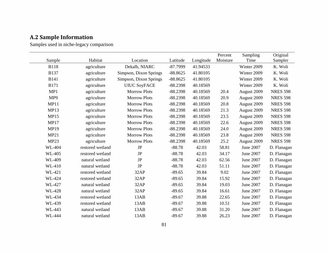
81
A.2 Sample Information Samples used in niche-legacy comparison
Sample Habitat Location Latitude Longitude
Percent
Moisture
Sampling
Time
Original
Sampler
B118 agriculture Dekalb, NIARC -87.7999 41.94533
Winter 2009 K. Woli
B137 agriculture Simpson, Dixon Springs -88.8625 41.80105
Winter 2009 K. Woli
B141 agriculture Simpson, Dixon Springs -88.8625 41.80105
Winter 2009 K. Woli
B171 agriculture UIUC SoyFACE -88.2398 40.18569
Winter 2009 K. Woli
MP1 agriculture Morrow Plots -88.2398 40.18569 20.4 August 2009 NRES 598
MP9 agriculture Morrow Plots -88.2398 40.18569 20.9 August 2009 NRES 598
MP11 agriculture Morrow Plots -88.2398 40.18569 20.8 August 2009 NRES 598
MP13 agriculture Morrow Plots -88.2398 40.18569 21.3 August 2009 NRES 598
MP15 agriculture Morrow Plots -88.2398 40.18569 23.5 August 2009 NRES 598
MP17 agriculture Morrow Plots -88.2398 40.18569 22.6 August 2009 NRES 598
MP19 agriculture Morrow Plots -88.2398 40.18569 24.0 August 2009 NRES 598
MP21 agriculture Morrow Plots -88.2398 40.18569 23.8 August 2009 NRES 598
MP23 agriculture Morrow Plots -88.2398 40.18569 25.2 August 2009 NRES 598
WL-404 restored wetland JP -88.78 42.03 58.81 June 2007 D. Flanagan
WL-405 restored wetland JP -88.78 42.03 34.17 June 2007 D. Flanagan
WL-409 natural wetland JP -88.78 42.03 62.56 June 2007 D. Flanagan
WL-410 natural wetland JP -88.78 42.03 51.11 June 2007 D. Flanagan
WL-421 restored wetland 32AP -89.65 39.84 9.02 June 2007 D. Flanagan
WL-424 restored wetland 32AP -89.65 39.84 15.92 June 2007 D. Flanagan
WL-427 natural wetland 32AP -89.65 39.84 19.03 June 2007 D. Flanagan
WL-428 natural wetland 32AP -89.65 39.84 16.61 June 2007 D. Flanagan
WL-434 restored wetland 13AB -89.67 39.88 22.65 June 2007 D. Flanagan
WL-439 restored wetland 13AB -89.67 39.88 10.51 June 2007 D. Flanagan
WL-443 natural wetland 13AB -89.67 39.88 31.20 June 2007 D. Flanagan
WL-444 natural wetland 13AB -89.67 39.88 26.23 June 2007 D. Flanagan
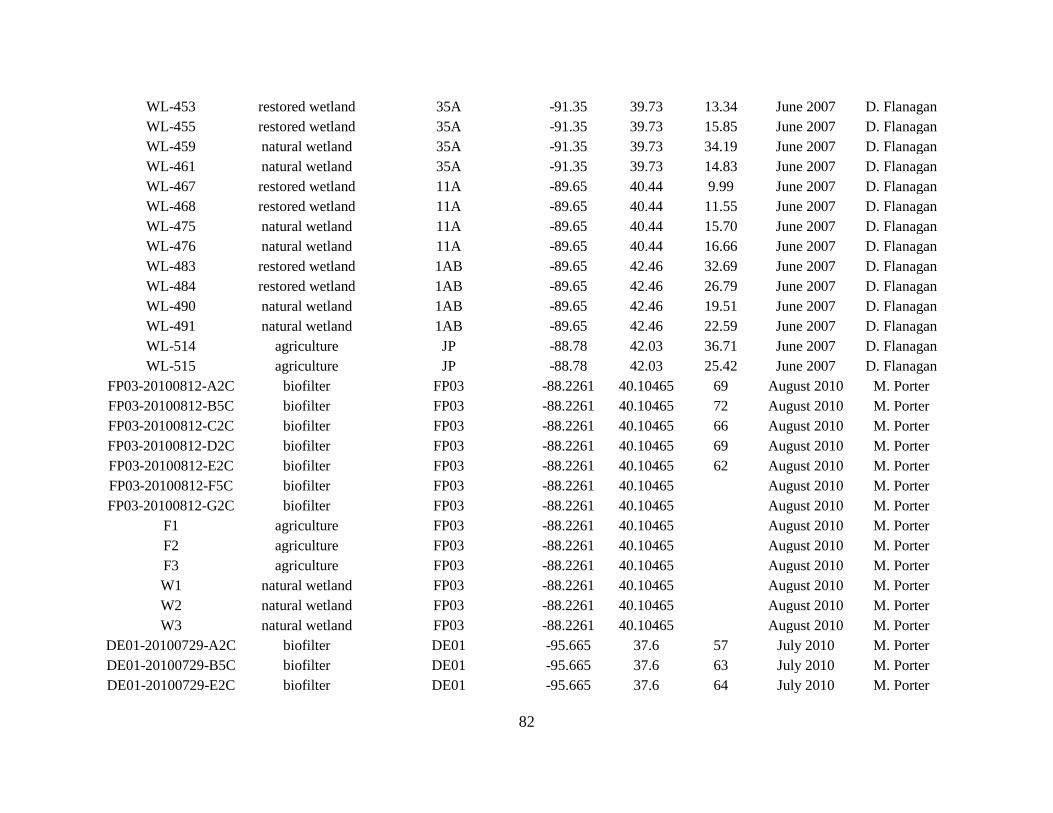
82
WL-453 restored wetland 35A -91.35 39.73 13.34 June 2007 D. Flanagan
WL-455 restored wetland 35A -91.35 39.73 15.85 June 2007 D. Flanagan
WL-459 natural wetland 35A -91.35 39.73 34.19 June 2007 D. Flanagan
WL-461 natural wetland 35A -91.35 39.73 14.83 June 2007 D. Flanagan
WL-467 restored wetland 11A -89.65 40.44 9.99 June 2007 D. Flanagan
WL-468 restored wetland 11A -89.65 40.44 11.55 June 2007 D. Flanagan
WL-475 natural wetland 11A -89.65 40.44 15.70 June 2007 D. Flanagan
WL-476 natural wetland 11A -89.65 40.44 16.66 June 2007 D. Flanagan
WL-483 restored wetland 1AB -89.65 42.46 32.69 June 2007 D. Flanagan
WL-484 restored wetland 1AB -89.65 42.46 26.79 June 2007 D. Flanagan
WL-490 natural wetland 1AB -89.65 42.46 19.51 June 2007 D. Flanagan
WL-491 natural wetland 1AB -89.65 42.46 22.59 June 2007 D. Flanagan
WL-514 agriculture JP -88.78 42.03 36.71 June 2007 D. Flanagan
WL-515 agriculture JP -88.78 42.03 25.42 June 2007 D. Flanagan
FP03-20100812-A2C biofilter FP03 -88.2261 40.10465 69 August 2010 M. Porter
FP03-20100812-B5C biofilter FP03 -88.2261 40.10465 72 August 2010 M. Porter
FP03-20100812-C2C biofilter FP03 -88.2261 40.10465 66 August 2010 M. Porter
FP03-20100812-D2C biofilter FP03 -88.2261 40.10465 69 August 2010 M. Porter
FP03-20100812-E2C biofilter FP03 -88.2261 40.10465 62 August 2010 M. Porter
FP03-20100812-F5C biofilter FP03 -88.2261 40.10465
August 2010 M. Porter
FP03-20100812-G2C biofilter FP03 -88.2261 40.10465
August 2010 M. Porter
F1 agriculture FP03 -88.2261 40.10465
August 2010 M. Porter
F2 agriculture FP03 -88.2261 40.10465
August 2010 M. Porter
F3 agriculture FP03 -88.2261 40.10465
August 2010 M. Porter
W1 natural wetland FP03 -88.2261 40.10465
August 2010 M. Porter
W2 natural wetland FP03 -88.2261 40.10465
August 2010 M. Porter
W3 natural wetland FP03 -88.2261 40.10465
August 2010 M. Porter
DE01-20100729-A2C biofilter DE01 -95.665 37.6 57 July 2010 M. Porter
DE01-20100729-B5C biofilter DE01 -95.665 37.6 63 July 2010 M. Porter
DE01-20100729-E2C biofilter DE01 -95.665 37.6 64 July 2010 M. Porter
83
FP07-20100812-A2C biofilter FP07 -88.2261 40.10465 66 August 2010 M. Porter
FP07-20100812-B2C biofilter FP07 -88.2261 40.10465 67 August 2010 M. Porter
FP07-20100812-C5C biofilter FP07 -88.2261 40.10465 71 August 2010 M. Porter
FP07-20100812-C5W biofilter FP07 -88.2261 40.10465
August 2010 M. Porter
FP07-20100812-D5C biofilter FP07 -88.2261 40.10465 63 August 2010 M. Porter
FP07-20100812-D5W biofilter FP07 -88.2261 40.10465
August 2010 M. Porter
FP07-20100812-E2C biofilter FP07 -88.2261 40.10465
August 2010 M. Porter


![WELCOME [d3pcsg2wjq9izr.cloudfront.net]...- High-performance nitrification and denitrification - with suspended and robust carrier-bound immobilised organisms, - for the main stream](https://img.pdfslide.net/doc/110x75/5f9fe4d0bd4e012e7b7a3cbb/welcome-high-performance-nitrification-and-denitrification-with-suspended.jpg)