Embed Size (px)
Citation preview

Performance Enhancement in Recently Deployed LTE
Wireless Networks
José Maria de Sousa Cardoso Marques
Thesis to obtain the Master of Science Degree in
Electrical and Computer Engineering
Supervisor: Prof. António José Castelo Branco Rodrigues
Examination Committee
Chairperson: Prof. Fernando Duarte Nunes
Supervisor: Prof. António José Castelo Branco Rodrigues
Members of Committee: Prof. João Miguel Duarte Ascenso
April 2014

ii

iii
To Leonor, Álvaro and Tomás

iv

v
Acknowledgements
Acknowledgements
Firstly, I would like to thank my two coordinators, Prof. António Rodrigues and Prof. Pedro Vieira, for
giving me the opportunity to study and learn more about a subject of my big interest. In addition, I also
want to thank for all your provided answers and ideas which helped me accomplish the proposed goals.
During the development of this dissertation I had the fortune of receiving many contributes from many
people, so to you all my most sincere gratitude.
I am also very obliged to my company Altran, especially to Rodrigo Cordeiro for his assistance,
comprehension, and time provided to finish this work. Also to Diana Salvador who helped me on some
chapters.
A special thanks to Fátima Almeida, who volunteered for the grammar review. I want to extend that
special thanks to Bruno Pires, who also reviewed my work and had the important mission to deliver this
work in person.
Also I want to give a special word to my friends, not only regarding the help during this dissertation, but
for all the times and for every support during my education.
Finally, my biggest appreciation to my parents and to my brother, for everything they give me and for
supporting me every time.

vi

vii
Abstract
Abstract
In telecommunications in general, optimization is a commonly used term. Mobile operators want to
provide a service with the best quality possible to their subscribers, and therefore are continually seeking
to improve the performance of their networks. When a new mobile technology comes, such as LTE
(Long Term Evolution), before being available to the public, it needs to be properly tested and optimized,
in order to ensure the desired quality of service. In this context, one will study a pilot LTE network in
which it was performed a Drive Test. The collected data from the Drive Test will be the input for the
optimization study to perform. For this study, it will also be examined LTE’s main features, highlighting
its evolution from the previous mobile generations. The DT will be analysed in detail, identifying the
areas where performance is poor and consequently will affect negatively the quality of service. Then, it
will be defined strategies to improve performance for the identified areas, applied to the current
network’s configuration. Finally, it will be simulated the addition of a new site to the network, analysing
the impact and if it is a justifiable option. This simulation uses propagation and performance models
obtained combining the real gathered data and the existing theoretical models.
Keywords
Optimization, Planning, LTE, Drive Test, KPIs,

viii
Resumo
Resumo
Nas telecomunicações em geral, otimização é um termo bastante recorrente. As operadoras pretendem
fornecer um serviço com a melhor qualidade possível aos seus subscritores, e portanto estão
continuamente à procura de melhorar a performance das suas redes. Quando surge uma nova
tecnologia móvel como é o caso do LTE (Long Term Evolution), antes de ser disponibilizada ao publico,
necessita de ser devidamente testada e otimizada, de modo a assegurar a qualidade de serviço
pretendida. Neste âmbito, será estudada uma rede piloto LTE, na qual se realizou um Drive Test. Os
dados recolhidos no Drive Test servirão de base ao estudo de otimização realizado. Para este estudo,
serão também analisadas as principais características do LTE, salientando a sua evolução face às
anteriores gerações móveis. O DT será detalhadamente analisado, identificando as áreas em que a
performance está aquém do que se pretenderia, e que consequentemente afetará a qualidade do
serviço prestado. Procurar-se-á posteriormente, encontrar estratégias de melhoramento de
performance para as áreas identificadas, aplicadas à sua atual configuração. Finalmente, será simulada
a introdução de um novo site, analisando o seu impacto e justificabilidade. Esta simulação usará
modelos de propagação e performance obtidos com base nos dados reais em conjunto com modelos
teóricos existentes.
Palavras-chave
Otimização, Planeamento, LTE, Drive Test, KPIs,

ix
Table of Contents
Table of Contents
Acknowledgements ................................................................................. v
Abstract ................................................................................................. vii
Resumo ................................................................................................ viii
Table of Contents ................................................................................... ix
List of Figures ........................................................................................ xi
List of Tables ......................................................................................... xiii
List of Acronyms .................................................................................. xiv
List of Software .................................................................................... xvi
1 Introduction .................................................................................. 1
1.1 Overview and Objectives ......................................................................... 2
1.2 Contents .................................................................................................. 3
2 State of the Art ............................................................................. 5
2.1 LTE .......................................................................................................... 6
2.1.1 Introduction ............................................................................................................ 6
2.1.2 System architecture ............................................................................................... 7
2.1.3 LTE Radio Interface ............................................................................................... 8
2.1.4 Physical Layer – Resource structure ................................................................... 15
2.1.5 Duplexing ............................................................................................................. 17
2.2 Key Performance Indicators (KPIs) ....................................................... 18
2.3 Models ................................................................................................... 19
2.3.1 Propagation Models ............................................................................................. 20
2.3.2 Performance Model ............................................................................................. 24
3 Drive Test ................................................................................... 26
3.1 Introduction ............................................................................................ 27
3.2 Results................................................................................................... 29
3.2.1 RSRP ................................................................................................................... 30

x
3.2.2 RSRQ .................................................................................................................. 31
3.2.3 SINR .................................................................................................................... 32
3.2.4 Downlink Throughput ........................................................................................... 33
3.2.5 Serving Cell (PCI) ................................................................................................ 34
3.3 Analysis ................................................................................................. 35
3.3.1 Coverage ............................................................................................................. 35
3.3.2 Quality .................................................................................................................. 36
3.3.3 Performance ........................................................................................................ 38
3.3.4 Serving Area ........................................................................................................ 40
3.4 Network Optimization ............................................................................ 42
4 Simulation .................................................................................. 45
4.1 Introduction ............................................................................................ 46
4.2 Simulation Models ................................................................................. 48
4.2.1 Propagation Models assessment and fitting ........................................................ 48
4.2.2 Performance Model assessment and fitting ........................................................ 52
4.3 Simulation Results ................................................................................. 53
4.3.1 Coverage prediction ............................................................................................ 53
4.3.2 Model Application ................................................................................................ 55
5 Conclusions ................................................................................ 59
References............................................................................................ 63
xi
List of Figures
List of Figures Figure 1.1 - Global data traffic in mobile networks, 2007-2013 [1]................................................ 2
Figure 2.1 - LTE Architecture. [7] .................................................................................................. 7
Figure 2.2 - OFDM spectral representation. [10] ........................................................................... 9
Figure 2.3 - OFDMA and SC-FDMA. [13] .................................................................................... 10
Figure 2.4 - Modulation Schemes. [15] ....................................................................................... 10
Figure 2.5 - Different MIMO configurations. [17] ......................................................................... 12
Figure 2.6 - Spatial multiplexing with CDD. [20] .......................................................................... 14
Figure 2.7 - Codebook indices for spatial multiplexing with two antennas, green background for two [16] .............................................................................................................. 14
Figure 2.8 - Multi User MIMO. two layers for two users. [20] ...................................................... 14
Figure 2.9 - TM6 Closed loop spatial multiplexing using a single transmission layer. [20] ......... 15
Figure 2.10 - LTE downlink physical resource grid based on OFDM. [12] .................................. 16
Figure 2.11 - LTE Frame Structure. [22] ..................................................................................... 16
Figure 2.12 - LTE resource structure. [23] .................................................................................. 17
Figure 2.13 - LTE FDD and TDD representation. [24] ................................................................ 17
Figure 2.14 - Castelo Branco airview. [31] .................................................................................. 20
Figure 2.15 - Parameters in the COST 231-Walfish-Ikegami model. [35] ................................... 23
Figure 2.16 - Throughput of a set of Coding and Modulation Combinations in LTE, assuming AWGN channels. [30] ........................................................................................ 25
Figure 2.17 - Approximating AMC with an Attenuated and Truncated form of the Shannon Bound. [30] ..................................................................................................................... 25
Figure 3.1 – RSRP. ..................................................................................................................... 30
Figure 3.2 – RSRQ. ..................................................................................................................... 31
Figure 3.3 – SINR. ....................................................................................................................... 32
Figure 3.4 - Downlink Throughput. .............................................................................................. 33
Figure 3.5 - Serving Cell (PCI). ................................................................................................... 34
Figure 3.6 - Bad coverage areas. ................................................................................................ 35
Figure 3.7- Average RSRP/Distance. .......................................................................................... 35
Figure 3.8 - Bad coverage area II. ............................................................................................... 36
Figure 3.9 - Bad coverage area III. .............................................................................................. 36
Figure 3.10 - Bad quality areas. .................................................................................................. 37
Figure 3.11 - SINR when RSRP < -105 dBm. ............................................................................. 37
Figure 3.12 - SINR when RSRP > -85 dBm. ............................................................................... 38
Figure 3.13 - Throughput/ RSRP. ................................................................................................ 38
Figure 3.14 - Throughput/ SINR. ................................................................................................. 39
Figure 3.15 - Average Throughput/ Distance. ............................................................................. 39
Figure 3.16 - Average serving distance/PCI. ............................................................................... 40
Figure 3.17 - Weak coverage Area. ............................................................................................ 43
Figure 3.18 - Lack of dominant cell. ............................................................................................ 43
Figure 3.19 - Cross Coverage area (pointed by the arrows). ...................................................... 44
Figure 4.1 – RSRP. ..................................................................................................................... 46

xii
Figure 4.2 – RSRQ. ..................................................................................................................... 46
Figure 4.3 – SINR. ....................................................................................................................... 46
Figure 4.4 – Throughput. ............................................................................................................. 46
Figure 4.5 - Drive Test RSRP measurements. ............................................................................ 48
Figure 4.6- Trendlines comparison between Models and DT data. ............................................ 50
Figure 4.7- Corrective factor (K). ................................................................................................. 50
Figure 4.8- Comparison between Model 4 plus corrective factor and DT data trendlines. ......... 51
Figure 4.9- SINR/RSRP relation and equation. ........................................................................... 52
Figure 4.10- Obtained Performance Model. ................................................................................ 53
Figure 4.11- RSRP before new site (scenario 1). ....................................................................... 54
Figure 4.12 - RSRP before new site (scenario 2). ...................................................................... 54
Figure 4.13- Simulation: RSRP scenario 1. ................................................................................. 57
Figure 4.14- Simulation: SINR scenario 1. .................................................................................. 57
Figure 4.15 – Simulation: Throughput scenario 1. ...................................................................... 57
Figure 4.16 – Simulation: RSRP scenario 2. ............................................................................... 58
Figure 4.17 - Simulation: SINR scenario 2. ................................................................................. 58
Figure 4.18 – Simulation: Throughput scenario 2. ...................................................................... 58

xiii
List of Tables
List of Tables Table 2.1 - CQI and MCS correlation. [16] .................................................................................. 11
Table 2.2 - Transmission Modes in LTE. [20].............................................................................. 13
Table 2.3 - Number of RB for different available bandwidth. ...................................................... 16
Table 2.4 - Okumura Hata validity ranges. .................................................................................. 21
Table 2.5 - Okumura-Hata model assumptions........................................................................... 22
Table 2.6 - COST 231 Extended Hata validity ranges. ............................................................... 22
Table 3.1 - Average Serving Distance / PCI. ............................................................................... 41
Table 3.2 - RF optimization. ........................................................................................................ 42
Table 4.1 - Current (average) measurements from weak coverage area. .................................. 47
Table 4.2 - Simulated Results comparison. ................................................................................. 55
Table 4.3- Simulation Results (percentage). ............................................................................... 56

xiv
List of Acronyms
List of Acronyms 2G – 2nd Generation of Mobile Network
3G – 3rd Generation of Mobile Network
3GPP – 3rd Generation Partnership Project
4G – 4th Generation of Mobile Network
AMC – Adaptive Modulation and Coding
AWGN – Additive White Gaussian Noise
BLER – Block Error Rate
BS – Base Station
CDD – Cyclic Delay Diversity
CP – Cyclic Prefix
CQI – Channel Quality Indicator
DL – Downlink
DT – Drive Test
E-UTRAN – Evolved Terrestrial Radio Access Network
eNB – Evolved Node B
EPC – Evolved Packet Core
ePDG – Evolved Packet Data Gateway
FDD – Frequency Division Duplex
GPRS – General Packet Radio Service
GSM – Global System for Mobile Communications
HSPA – High-Speed Packet Access
HSS – Home Subscriber Server
IP – Internet Protocol
ISI – Intersymbol Interference
KPI – Key performance Indicator
LTE – Long Term Evolution
MCS – Modulation and Coding Scheme
MIMO – Multiple Input Multiple Output
MME – Mobility Management Entity
OFDM – Orthogonal Frequency–Division Multiplexing
OFDMA – Orthogonal Frequency–Division Multiple Access
PCI – Physical Layer Cell Identity
PCRF – Policy Control and Charging Rules
P-GW – Packet Data Network Gateway
PMI – Precoding Matrix Indicators
PRB – Physical Resource Blocks
QAM – Quadrature Amplitude Modulation
QoS – Quality of Service
QPSK – Quadrature Phase-Shift Keying
RB – Resource Block

xv
RE – Resource Element
RI – Ranks Indications
RSRQ – Reference Signal Received Quality
RSRP– Reference Signal Received Power
S-GW – Serving Gateway
SC-FDMA – Single Carrier Frequency Division Multiple Access
SIMO – Single Input Multiple Output
SINR – Signal to Interference plus Noise Ratio
SISO – Single Input Single Output
TDD – Time Division Duplex
TDMA – Time Division Multiple Access
TTI – Time Transmission Interval
UE – User Equipment
UL – Uplink
UMTS – Universal Mobile Telecommunications Systems

xvi
List of
List of Software Microsoft Excel
MapInfo Professional
Microsoft Word

1
Chapter 1
Introduction
1 Introduction
This chapter gives an overview for the present dissertation. It addresses the goals and motivations to
conduct such study and provides the structure in which it is organized.

2
1.1 Overview and Objectives
Since ever communication has been part of the human existence. People want to be in touch, all the
time, and not only with the ones near them. To enable this constant urge and due to his inherent
curiosity, man constantly pursues new, faster and better ways to communicate.
In this context comes Telecommunications. In a simplified definition, it is the exchange of information
between two or more individuals over distance. Typically, it is associated with the use of technology,
and information being sent through electrical signals or electromagnetic waves.
Mobile communications are a key part of that, and they are also the main theme of the present
dissertation.
In recent years, the constant growth of the exchange of information pushed telecommunication
engineers to develop new and better techniques, in order to provide an answer to that increasing
demand. Also, communication habits and means are continuously changing, and today one assists to
an increasingly mobile world. So, when Internet was brought from computers to people’s pockets too, it
represented a huge growth of mobile traffic. In this context comes the smartphone. It is undoubtedly the
responsible for that data growth and still more and more people are getting one, especially in the
emerging markets and highly populated countries like China and India.
The following figure illustrates the evolution of mobile traffic between 2007 and 2013:
Figure 1.1 - Global data traffic in mobile networks, 2007-2013 [1]
The path to LTE started with GSM (Global System for Mobile Communications) or 2G [2] and it was
design to carry voice traffic, with data communication support added later via GPRS (General Packet
Radio Services) and EDGE (Enhanced Data rates for GSM Evolution or EGPRS). This system enabled
voice communications to go wireless[3] and it is the global standard for mobile communications with
over 90% market share, and is available in over 219 countries. The following system[3], the third
generation (3G) Universal Mobile Telecommunications System (UMTS) brought more capacity to the
mobile network, allowing new multimedia services. The UMTS supports a maximum theoretical data
rate of 42 Mbps [4] when High Speed Packet Access (HSPA+) is implemented.

3
The change of costumers’ habits and the previous stated data traffic growth, demanded a new evolution
for the mobile communication systems, and LTE (Long Term Evolution) was the response. Being
commercially advertised as “4G”, it intends to be a clear improvement over previous mobile
technologies, providing even higher data rates, lower latency and better spectral efficiency.
Throughout the present dissertation LTE will be detailed and studied, in order to comprehend its
characteristics, its differences over the previous systems and how the defined improvements were
achieved through different techniques.
Before a new mobile system is available to the general public, it has to be properly tested and enhanced,
by the mobile operators. In this phase – deployment – it is essential to ensure coverage to the target
areas, assess the provided user experience and performance, and also assure that the existing systems
are not affected by the new one. An important tool that is frequently used to help in this process is Drive
Testing. It gathers measurements of the network’s actual conditions that can be later analysed.
The purpose of the present dissertation is precisely to find strategies of performance enhancement that
can be applied to the deployment phase of a LTE network. These strategies will be based on provided
data from a Drive Test performed in Castelo Branco, Portugal. Also is intended the establishment of
propagation and performance models which can be used for simulating alternative scenarios with
different equipment setups.
1.2 Contents
This thesis is composed of 5 chapters. Each chapter contents can be summarized by:
Chapter 1 – Introduction:
o Problem description and dissertation purposes
Chapter 2 – State of the Art
o LTE technology features overview
o KPIs overview and formulas
o Propagation models: formulas and validity ranges
o LTE system level performance model
Chapter 3 – Drive Test Analysis
o Drive Test overview
o Drive Test analysis:
o Proposed optimizations
Chapter 4 – Simulation
o Model establishment and fitting to the specific area in study
o Simulation of alternative scenarios, using different frequency bands and additional
equipment.
o Simulation results analysis and comparison with the real conditions.

4
Chapter 5 – Conclusions
o Summary of the performed study
o Evaluation of the obtained results

5
Chapter 2
State of the Art
2 State of the Art
In this chapter it will be studied and detailed the relevant subjects in which the work is based on. This
study will allow a better knowledge for each subject, before obtaining any of the intended results.
6
2.1 LTE
2.1.1 Introduction
Before entering in technical details about LTE technology and networks it’s important to understand
what the motivations to develop this new mobile technology were and targets established by the 3GPP
(3rd Generation Partnership Project).
In mobile communications business the companies are constantly looking for new technologies and
ways to provide costumers new or improved services, possibly at a lower cost, in order to attract more
subscribers. So, as stated in [5] the key drivers to a new mobile system are:
Staying competitive;
Services (better provisioning of old services as well as provisioning of new services);
Cost (more cost-efficient provisioning of old services as well as cost-effective provisioning
of new services).
There were several factors that motivated the development of LTE, such as the growth of fixed
communications capacity with the implementation of optical fiber solutions and the offer of wireless (Wi-
Fi) services with also high capacity.
With these in mind, at the start of 2005 [3] and [6] the 3GPP define the following targets to LTE:
All IP network: the LTE system should be packet switched domain optimized;
In terms of latency must be below 10ms for the LTE radio round trip and access delay
lower than 300ms;
The data rates should represent a major step from the previous 3G HSPA networks, so
the peak rate should be higher than 50Mbps for the uplink, and higher than 100 Mbps for
the downlink.
High spectral efficiency;
Interoperability with existing mobile systems (GSM, UMTS)
Good level of mobility and security ensured;
Improved terminal power efficiency;
Frequency allocation flexibility with 1.25/2.5, 5, 10, 15 and 20 MHz allocations;
Simplified architecture
Even the name, “Long Term Evolution”, emphasizes the goal of a clear evolution from the UMTS system.
So, from a simplistic point of view, LTE objective is to provide higher data rates to users, in addition to
a lower latency. The combination of these two factors can potentiate by far the offer of applications and
services for mobile phones and other devices with mobile connectivity, such as video streaming,
videoconference, gaming, VoIP and many more, which ultimately will provide increasing profits for all
mobile industry.

7
2.1.2 System architecture
In opposition to the former mobile technologies, LTE was planned to support only packet switching
services: all IP network. This new architecture is designed to optimize network performance, improve
cost-efficiency and facilitate the introduction of mass-market IP-based services.
Figure 2.1 - LTE Architecture. [7]
The LTE system, as shown in previous figure, is composed by two kind of networks:
Evolved Universal Terrestrial Radio Access Network (E-UTRAN)
Evolved Packet Core (EPC)
2.1.2.1 Access network: E-UTRAN
The E-UTRAN consists of a network of e-NoodBs (eNBs). It has a flat architecture since there is not any
centralized controller, unlike the previous mobile generations. The e-NoodBs are linked with each other
through an X2 interface and connected with the EPC through an S1 interface [8]
The E-UTRAN is responsible for all radio functions of the network, such as:
Radio Resource Management: responsible to manage the radio bearers functions such as
radio bearer control, radio admission control, radio mobility control, scheduling and dynamic
allocation to UEs in both uplink and downlink.
User Data Encryption: encrypts all user data, in order to provide better security and prevent
unwanted access.
Header Compression: compresses IP packets headers to increase efficiency of the radio
interface.
Connectivity to the EPC: responsible for the communication with the EPC through signalling.
This simple, flat and integrated architecture for the E-UTRAN aims for an improved efficiency,
reduced latency and also reduced cost for the operators.

8
2.1.2.2 Evolved Packet Core
The EPC is the latest evolution of the 3GPP core network architecture. [9] [10] As stated before it is an
all IP Network, in contrast with 3G and 2G core networks, so it no longer uses circuit-switched domain,
and was designed to support higher throughput and lower latency Radio Access Networks (RAN’s) as
well as the former RANs (2G and 3G).
The components of the EPC are:
Mobility Management Entity (MME): it is the most important component in the EPC. It
handles the signalling between the user and the Core Network. The MME functions are
authentication, mobility management, security and retrieval of subscription information from
the Home Subscriber Server (HSS).
Home Subscriber Server (HSS): is a database containing all user subscription information,
and operator offered services. It also provides support functions in mobility management, call
and session setup, user authentication and access authorization.
Serving Gateway (S-GW): is responsible for forwarding user data packets, and it is also
mobility anchor for the user plane during inter-eNodeB handovers and as the anchor for
mobility between LTE and other 3GPP technologies.
Public Data Network Gateway (P-GW): is responsible for IP address allocation to the user
and also to enforce QoS according to the rules from Policy Control and Charging Rules
Function (PCRF). The PCRF is responsible for applying various operators’ policies on the
network, like guaranteed QoS or defining what bit rate should be provisioned to a user. The P-
GW also assures interoperability with other non-3GPP technologies such as WIMAX and
CDMA2000 networks.
2.1.3 LTE Radio Interface
This section will address the main aspects of LTE radio interface, in particular multiple access
techniques used, transmission schemes and multiple antenna transmission
2.1.3.1 Multiple Access
Multiple access is essential for mobile communications. It allows several users access to the network
and use it simultaneously. In LTE, as stated previously, one of the major goals is to seek for a better
usage of the spectrum, so efficiency assumes a major significance in the choice of multiple access
techniques. Other relevant aspect taken in account is flexibility between users with different needs and
usage of the network: for example checking the e-mail or watching a video on Youtube requires very
different bandwidths. In addition it must support multi-antenna techniques too, which will be described
in more detail, ahead in this chapter.
After all these and more considerations, although the 3GPP looked at other options, quickly the choice
for LTE multiple access was SC-FDMA in the Uplink and OFDMA in the Downlink [6]. Both are variants
from OFDM (Orthogonal Frequency Division Multiplex):

9
Figure 2.2 - OFDM spectral representation. [10]
These techniques can be described as following:
Orthogonal Frequency Division Multiple Access (OFDMA) [6] [11] [12]: The principle of the OFDMA is
based on the use of narrow, mutually orthogonal sub-carriers, each one spaced 15 KHz between each
other (in the case of LTE), and at the sampling instant of a single sub-carrier, all the others have zero
value (as seen in the previous figure), avoiding crosstalk. The data to be transmitted by the user is
divided in multiple data sub-fluxes, modulated into different OFDMA sub-carriers (generating data
symbols), which will simultaneously be transmitted, generating this way a high speed data flux. Each
sub-carrier is independently coded and modulated which provides a great adaptability to the channel
conditions. This is called Adaptive Modulation and Coding and will be described with more detail ahead.
The sub-carriers are received by multiple users simultaneously, providing this way a multiple access
scheme: this is what differentiates OFDMA from OFDM, and it’s done with the use of TDMA (Time
Division Multiple Access) which means that groups of sub-carriers are dynamically assigned to each
user, during a specific time slot. Finally, another significant aspect of OFDMA is the introduction of a
guard prefix, named cyclic prefix (CP), in between the sub-carriers that, in addition to a long symbol
time, provides great robustness against inter-symbolic interference (ISI), caused by the existence of
multipath in this kind of radio transmission. There are two kinds of cyclic prefix, the normal CP and the
extended CP. the normal CP has the duration of 5 µs and the extended CP has 17 µs which is used
when the multipath effect is heavier.
Single Carrier-Frequency Division Multiple Access (SC-FDMA): The SC-FDMA technique is very similar
to OFDMA but was chosen to the uplink transmission by virtue of some important benefits. The main is
the lower Pick to Average Ratio (PAR) when comparing with OFDMA. The uplink signal is generated by
the users’ mobile terminal, so the power efficiency becomes a crucial aspect, in consequence of the
limitations of mobile batteries and also reduces the cost of the power amplifier. SC-FDMA can benefit
from the advantages stated previously for the OFDMA with the important addition of low PAR. For the
transmission process SC-FDMA also splits the available bandwidth in sub-carriers with cyclic prefix to
avoid ISI interference, but differentiates itself from OFDMA because in the first scheme the transmission

10
of the “N” different data symbols occurs in parallel (in the time domain), and in SC-FDMA it occurs in
series (each one at a time) but at “N” times the rate. In order to illustrate this and for a better perception
check figure 2.3. This difference is what justifies the prefix “Single Carrier” in opposition to OFDMA
multiple carrier scheme. This is also what justifies the lower PAR of this scheme.
Figure 2.3 - OFDMA and SC-FDMA. [13]
2.1.3.2 Adaptive Modulation and Coding (AMC)
The characteristics and conditions of the radio link between the UE and E-NodeB are continuously
changing due to its wireless nature. So depending on the existence or not of Line of sight, the distance,
multi-path reflexion, interference, noise level, it is essential to adapt the link to this conditions. In order
to dynamically optimize the data rate and coverage to those varying conditions, LTE uses Adaptive
Modulation and Coding. [2] [14]
There are essentially two ways to perform link adaptation in LTE:
Modulation Scheme: there are 3 modulation schemes to be used: QSPK (Quadrature Phase-Shift Key),
16-QAM and 64-QAM (Quadrature Amplitude Modulation). The following figure illustrates the number
of bits per symbols of each scheme:
Figure 2.4 - Modulation Schemes. [15]
QPSK is the most robust to interference and bad channel conditions, but consequently offers the lower
bit rate. In contrast the 64-QAM allows the higher bit rates in LTE, but requires the best conditions in
terms of SINR, by being the most prone to errors due to interference.
Code Rate: For a given modulation scheme, several code ratios can be chosen according to the radio
11
conditions. The higher code rate is used in the better radio conditions and the lower code rate when
experiencing poor conditions.
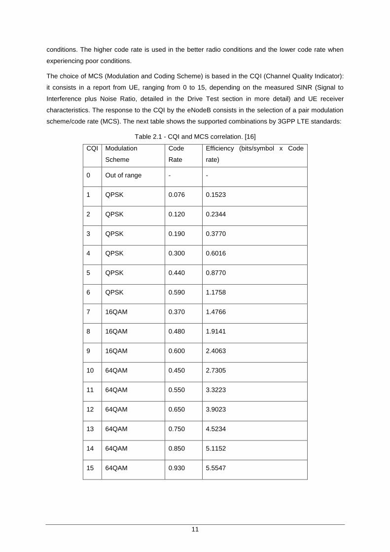
The choice of MCS (Modulation and Coding Scheme) is based in the CQI (Channel Quality Indicator):
it consists in a report from UE, ranging from 0 to 15, depending on the measured SINR (Signal to
Interference plus Noise Ratio, detailed in the Drive Test section in more detail) and UE receiver
characteristics. The response to the CQI by the eNodeB consists in the selection of a pair modulation
scheme/code rate (MCS). The next table shows the supported combinations by 3GPP LTE standards:
Table 2.1 - CQI and MCS correlation. [16]
CQI Modulation
Scheme
Code
Rate
Efficiency (bits/symbol x Code
rate)
0 Out of range - -
1 QPSK 0.076 0.1523
2 QPSK 0.120 0.2344
3 QPSK 0.190 0.3770
4 QPSK 0.300 0.6016
5 QPSK 0.440 0.8770
6 QPSK 0.590 1.1758
7 16QAM 0.370 1.4766
8 16QAM 0.480 1.9141
9 16QAM 0.600 2.4063
10 64QAM 0.450 2.7305
11 64QAM 0.550 3.3223
12 64QAM 0.650 3.9023
13 64QAM 0.750 4.5234
14 64QAM 0.850 5.1152
15 64QAM 0.930 5.5547

12
In order to report a certain CQI the UE measures what MCS combination that ensures a BLER (Block
Error Rate) lesser than 10%.
2.1.3.3 Multiple Antennas Techniques (MIMO)
The multi-input multi-output (MIMO) is a technique used in mobile technologies in order to improve
spectral efficiency, obtain higher data rates and enhanced coverage. It consists in the use of multiple
antennas in both transmitter and receiver. LTE takes advantage of MIMO to achieve the proposed goals
in terms of peak data rates without requiring more transmitting power or bandwidth.[17][18][19]
Essentially MIMO provides different kinds of gains:
Array Gain: improvement of the average signal to noise ratio (SINR) using the same
transmission power. It is obtained by coherent combining of various signals.
Power Combining Gain: can be described by the following expression10 log(𝑁) 𝑑𝐵. N
represents the number of multiple transmitting antennas.
Spatial Multiplexing Gain: improvement of the data throughput using the same bandwidth
and transmission power.
Diversity Gain: improvement of the average signal quality, making the radio link more robust
against the fading effects which are inherent to a wireless connection.
Also, can be presented in different configurations, which are better illustrated by the following figure:
Figure 2.5 - Different MIMO configurations. [17]
The “S” stands for Single, and the “M” for multiple, so there are 4 possibilities:
Single Input Single Output: basically consists in the no use of MIMO
Single Input Multiple Output: only one antenna in the transmission and more than one
present in the receiver
Multiple Input Single Output: more than one antennas in the transmission and only one
present in the receiver
Multiple Input Multiple Output: more than one antennas in both transmission and reception

13
2.1.3.4 Transmission Modes
Based on the introduction of MIMO technique, there were created different Transmission Modes.
Each one represents different kind of gains and propagation conditions, with specific goals and
characteristics. The 3GPP release 8 describes seven different TM’s: [20]
Table 2.2 - Transmission Modes in LTE. [20]
Transmission Mode Description
1 Single transmit antenna
2 Transmit diversity
3 Open loop spatial multiplexing with cyclic
delay diversity (CDD)
4 Closed loop spatial multiplexing
5 Multi-user MIMO
6 Closed loop spatial multiplexing using a
single transmission layer
7 Beamforming
TM1 - Single transmit antenna: in this case that only one antenna is transmitting (SISO and SIMO)
TM2 – Transmit diversity: This is the default MIMO transmission mode. In this case the same signal is
transmitted through multiple antennas, but with different coding and frequency resources, resulting in a
better Signal to Noise Ratio (SNR). The capacity remains unchanged. Transmit diversity is used in
cases such as when spatial multiplexing isn’t possible, as a fallback option.
TM 3 – Open loop spatial multiplexing (with CDD) : In this mode, spatial multiplexing of 2 or 4
transmission layers1 (according to the number of transmitting antennas) is used, improving the data rate
to higher values. So in this mode the goal is to provide higher capacity to the transmission. In order to
create frequency diversity between each signal transmitted by different antennas, a specific delay is
added to those signals: Cyclic delay diversity (CDD). The following picture illustrates this technique.
1 Transmission layer refers to a data flux transmitted by one Antenna. It is equal to the number of
transmitting antennas.

14
Figure 2.6 - Spatial multiplexing with CDD. [20]
TM 4 – Closed loop spatial multiplexing: this mode also supports 2 or 4 Transmission layers (with 2 or
4 antennas), in order to improve the data rate. The major difference from the previous mode relates with
the transmission of cell-specific reference signals over various resource elements and timeslots. The
response from the UE gives feedback regarding the channel situation and the precoding to be used.
This is done by selecting one index (precoding matrix indicator) from a matrix table codebook, which is
known by both transmitter and receiver. The following picture illustrates this table for the 2 layer case:
Figure 2.7 - Codebook indices for spatial multiplexing with two antennas, green background for two
[16]
TM 5 – Multi-User MIMO: this mode is very similar with the last one (Closed Loop Spatial Multiplexing)
but with the difference that each layer is dedicated for each UE.
Figure 2.8 - Multi User MIMO. two layers for two users. [20]
TM 6 – Closed loop spatial multiplexing using a single transmission layer: this mode works very similarly

15
to TM4, with the major difference of only being used one spatial layer2. The UE also sends feedback
about the channel, and, based in the matrix from figure 2.7 for the one layer case, a codebook index is
chosen to be sent to the BS. The precoded signal is then sent by all antennas.
Figure 2.9 - TM6 Closed loop spatial multiplexing using a single transmission layer. [20]
TM 7- Beamforming: This mode has the goal to improve the coverage, using the beamforming
technique. It consists in the power concentration of the transmitted signal and phase modification, in
order to obtain a constructive sum of the signal in reception.
2.1.4 Physical Layer – Resource structure
[12] [21] LTE’s basic downlink structure can be seen as time-frequency-grid, where Resource Blocks
(RBs) are allocated. On the other hand, one of the previous stated (downlink) OFDMA subcarriers,
alongside with a symbol (QPSK, 16-QAM or 64-QAM) constitutes a Resource Element (RE). In the
frequency domain, the RBs have a total size of 180 KHz, and, as seen before, the subcarrier spacing is
15 KHz, which means that a RB contains 12 RE. In the time domain, a OFDM symbol has the duration
of 1/∆f+CP (cyclic prefix), and the RB has the duration of 0.5 ms (called a Time Slot), being this way
able to accommodate 7 OFDM symbols with normal CP (in the case of extended CP 6 symbols). The
following picture illustrates the LTE physical layer and helps to understand this structure:
2 Spatial layer refers to a data stream with unique information, not included in any of the other layers
16
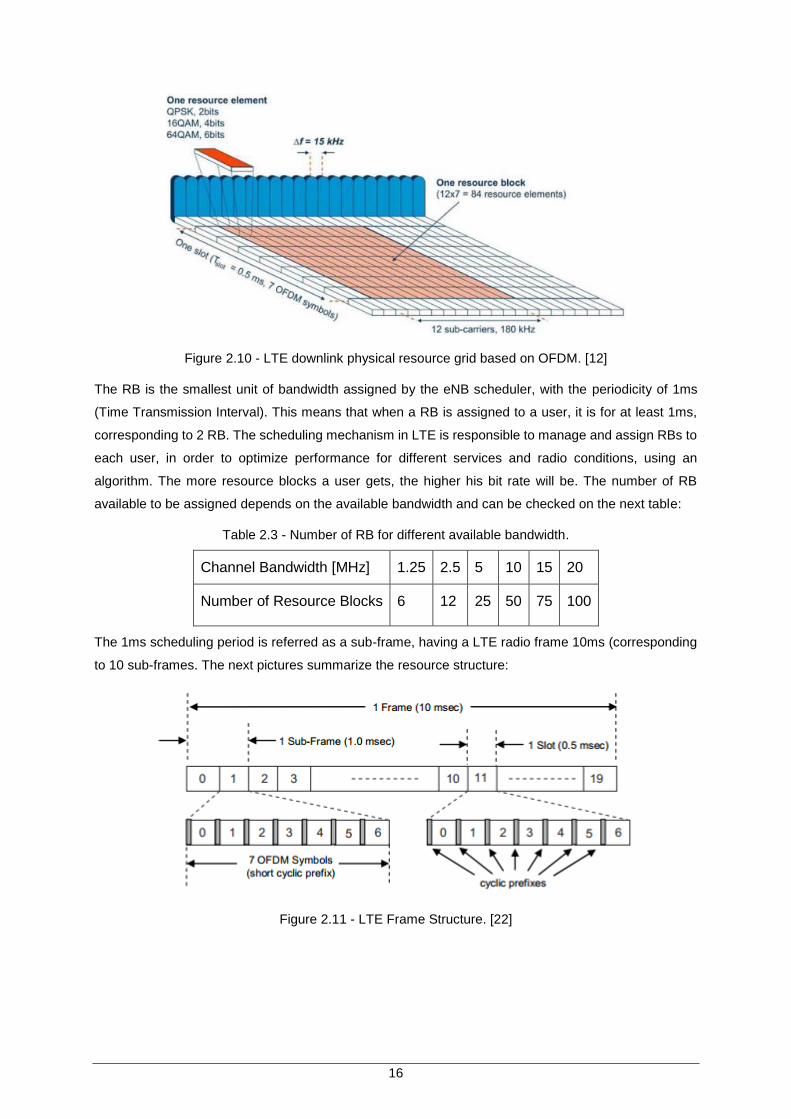
Figure 2.10 - LTE downlink physical resource grid based on OFDM. [12]
The RB is the smallest unit of bandwidth assigned by the eNB scheduler, with the periodicity of 1ms
(Time Transmission Interval). This means that when a RB is assigned to a user, it is for at least 1ms,
corresponding to 2 RB. The scheduling mechanism in LTE is responsible to manage and assign RBs to
each user, in order to optimize performance for different services and radio conditions, using an
algorithm. The more resource blocks a user gets, the higher his bit rate will be. The number of RB
available to be assigned depends on the available bandwidth and can be checked on the next table:
Table 2.3 - Number of RB for different available bandwidth.
Channel Bandwidth [MHz] 1.25 2.5 5 10 15 20
Number of Resource Blocks 6 12 25 50 75 100
The 1ms scheduling period is referred as a sub-frame, having a LTE radio frame 10ms (corresponding
to 10 sub-frames. The next pictures summarize the resource structure:
Figure 2.11 - LTE Frame Structure. [22]

17
Figure 2.12 - LTE resource structure. [23]
2.1.5 Duplexing
LTE supports both FDD (Frequency Division Duplex) and TDD (Time Division Duplex). To clarify the
difference between these techniques, in FDD, downlink and uplink traffic is transmitted at the same time
in separate frequency bands. On the contrary, in TDD the transmission in downlink and uplink is
discontinuous and both use the same frequency band. FDD is currently the most used technique,
corresponding to more than 90% of the word’s available mobile frequencies. [12] In fact, operators often
use more than half of their resources in the downlink, and if TDD is used, it will need more sites to cover
the same area when compared to FDD: in a 3/1 Downlink/Uplink ratio, TDD uses approximately more
20% sites than FDD.
The following figure shows the representation of the two techniques:
Figure 2.13 - LTE FDD and TDD representation. [24]

18
Some of the terms in the previous picture refer to LTE TDD frame structure which is different from the
one presented in the preceding chapter (LTE Physical Layer). The frame consists of two half-frames of
equal length, containing 10 or 8 slots plus 3 special fields (present in the previous picture), each slot
with 0.5ms duration:
DwPTS: Downlink pilot time slot
UpPTS: Uplink pilot time slot
GP: Guard period
These 3 special fields combined always have 1ms of duration, but individually length can vary,
depending on the uplink/downlink configuration. [25]
2.2 Key Performance Indicators (KPIs)
In this section the goal is to describe the KPIs (Key Performance Indicators) related to mobile systems
and in particular the ones to evaluate in a LTE network. [27] [28] [29].
First, in telecommunications, a KPI is a performance measurement that is used to evaluate, monitor and
assess about the network performance, which determines what kind of service quality can be provided
to a costumer. Specifying to the case of LTE, it’s important for the operators to check about the
performance that can be provided both at the time of a commercial launch, and after the deployment. In
order to do this there are two main data sources: Field Testing (Drive Tests for example) and statistical
analyzes.
For the first phase, before the commercial launch to costumers, once that there is no traffic in the
network, the only option is to perform Field Testing, such as Drive Test, Walk Tests or Stationary Tests.
Then, after the launch, even if the traffic is very low (which is expected), statistical analyses can be
introduced as well. For the first phase the main aspects to be evaluated are the coverage area and
performance. Since the present work is based in this type of testing, in particular Drive test, this will be
described in more detail.
There are 5 categories in which the KPIs can be categorized:
Accessibility: E-RAB Establishment Success Rate
Throughput: Downlink and Uplink User Throughput
Mobility: Handover Success Rate (intra-system)
Retainability: E-RAB Retainability rate
Latency: Round Trip Time (Ping)
According to [29] these KPIs can be described and calculated as:
E-RAB Establishment Success Rate: Probability success rate for E-RABs establishment.
Successful attempts compared with total number of attempts for the different parts of the E-
RAB establishment.
o Formula:

19
𝑁𝑢𝑚𝑏𝑒𝑟 𝑜𝑓 𝑠𝑢𝑐𝑐𝑒𝑠𝑠𝑓𝑢𝑙 𝐸−𝑅𝐴𝐵 𝑒𝑠𝑡𝑎𝑏𝑙𝑖𝑠ℎ𝑚𝑒𝑛𝑡𝑠
𝑁𝑢𝑚𝑏𝑒𝑟 𝑜𝑓 𝑟𝑒𝑐𝑒𝑖𝑣𝑒𝑑 𝐸−𝑅𝐴𝐵 𝑒𝑠𝑡𝑎𝑏𝑙𝑖𝑠ℎ𝑚𝑒𝑛𝑡 𝑎𝑡𝑡𝑒𝑚𝑝𝑡𝑠 (1)
Throughput (Downlink and Uplink): A KPI that shows how E-UTRAN impacts the service
quality provided to an end-user. Given by the Payload data volume on IP level per elapsed
time unit on the Uu interface.
o Formulas:
𝐼𝑃 𝑇ℎ𝑟𝑜𝑢𝑔ℎ𝑝𝑢𝑡 𝑖𝑛 𝐷𝐿 = 𝑇ℎ𝑝𝑉𝑜𝑙𝐷𝑙 / 𝑇ℎ𝑝𝑇𝑖𝑚𝑒𝐷𝑙 (𝑘𝑏𝑖𝑡𝑠/𝑠) (2)
𝐼𝑃 𝑇ℎ𝑟𝑜𝑢𝑔ℎ𝑝𝑢𝑡 𝑖𝑛 𝑈𝐿 = 𝑇ℎ𝑝𝑉𝑜𝑙𝑈𝑙 / 𝑇ℎ𝑝𝑇𝑖𝑚𝑒𝑈𝑙 (𝑘𝑏𝑖𝑡𝑠/𝑠) (3)
Note: ThpVolDl is the volume on IP level and the ThpTimeDl is the time
elapsed on Uu for transmission of the volume included in ThpVolDl. The same
applies to the UL case.
Handover Success Rate: A KPI that shows how E-UTRAN Mobility functionality is working.
o Formula:
𝐻𝑂.𝐸𝑥𝑒𝑐𝑆𝑢𝑐𝑐×𝐻𝑂.𝑃𝑟𝑒𝑝𝑆𝑢𝑐𝑐
𝐻𝑂.𝐸𝑥𝑒𝑐𝐴𝑡𝑡×𝐻𝑂.𝑃𝑟𝑒𝑝𝐴𝑡𝑡 (4)
Note: “Entering preparation phase” is defined as the point of time when the
source eNB attempts to prepare resources for an UE in a neighboring cell.
“Success of execution phase” is defined as the point of time when the source
eNB receives information that the UE is successfully connected to the target
cell.
E-RAB Retainability: A measurement that shows how often an end-user abnormally loses an
E-RAB during the time the E-RAB is used. Number of E-RABs with data in a buffer that was
abnormally released, normalized with number of data session time units.
o Formula:
𝑁𝑢𝑚𝑏𝑒𝑟 𝑜𝑓 𝑎𝑏𝑛𝑜𝑟𝑚𝑎𝑙𝑙𝑦 𝑟𝑒𝑙𝑒𝑎𝑠𝑒𝑑 𝐸−𝑅𝐴𝐵 𝑤𝑖𝑡ℎ 𝑑𝑎𝑡𝑎 𝑖𝑛 𝑎𝑛𝑦 𝑜𝑓 𝑡ℎ𝑒 𝑏𝑢𝑓𝑓𝑒𝑟𝑠
𝐴𝑐𝑡𝑖𝑣𝑒 𝐸−𝑅𝐴𝐵 𝑇𝑖𝑚𝑒
[𝑟𝑒𝑙𝑒𝑎𝑠𝑒𝑠𝑠𝑒𝑠𝑠𝑖𝑜𝑛 𝑡𝑖𝑚𝑒]⁄
(5)
Latency: Time from reception of IP packet to transmission of first packet over the Uu.
o Formula:
𝐿𝑎𝑡𝑒𝑛𝑐𝑦_𝐷𝐿 = ∑ 𝑇_𝐿𝑎𝑡_𝐷𝐿 (𝑠) / # 𝑠𝑎𝑚𝑝𝑙𝑒𝑠 (6)
Note: T_Lat is defined as the time between reception of IP packet and the
time when the eNodeB transmits the first block to Uu.
2.3 Models
Mobile communication systems can prove to be challenging when one attempts to predict and estimate
the signal’s strength, phase, multipath reflections and other variables, at a certain position. The
propagation conditions and environment are continuously changing, as well as the UE position (which
can be considered both receiver and transmitter depending on the link direction). Also, the link path
varies from a line of sight situation, to one with considerable obstruction from buildings, vegetation or
the actual terrain orography. The distance to the BS can likewise range between a few meters to some
kilometres.
All these factors contribute to the complex task of establishing a model that describes accurately the
way radio waves behave and propagate under the different conditions mentioned. It has been a
20
particular interesting problem and subject of significant investigation in the recent years.
Taken advantage of that work and the already existing models, a new one, based in live measurements
from a Drive Test, will be established. The purpose of this model is to replicate the observed propagation
conditions, estimating an expected received power by the UE given a certain distance of the serving
BS. The starting point will be the study of Propagation Models and chose the ones that both respect the
experienced conditions in the DT, and matches, with minimum error, the measured results. The intended
result should be a model that estimates accurately the received signal by an UE, on a LTE network with
similar setup and environment with the one from the DT (Castelo Branco).
In addition, a Link Level Performance Model will also be extrapolated from the Drive Test results. This
model should determine the obtained Throughput, at a given SINR, which sets which MCS (Modulation
and Coding Scheme, detailed in section Radio Interface) can be used with acceptable BLER (Bit Error
Rate). The comparison model, [30], also approximate the throughput over a channel with a given SNR,
when using link adaptation (AMC), but in this case using equations. This model will be detailed in the
next section “Performance Models”.
2.3.1 Propagation Models
In short, the objective is essentially to evaluate the power reduction (path loss) of the signal in its path
between the serving BS and the UE (considering the Downlink case).
A RF propagation model can be described as a mathematical formulation (equation), which
characterizes radio wave propagation as a function of distance, frequency, obstructions, terrain and
many other variables. Different models have different approaches, but all are based by both empirical
measures and observations, and theoretical considerations.
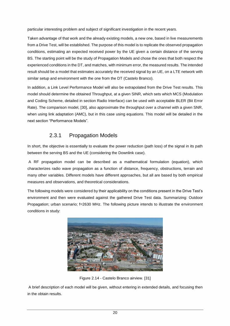
The following models were considered by their applicability on the conditions present in the Drive Test’s
environment and then were evaluated against the gathered Drive Test data. Summarizing: Outdoor
Propagation; urban scenario; f=2630 MHz. The following picture intends to illustrate the environment
conditions in study:
Figure 2.14 - Castelo Branco airview. [31]
A brief description of each model will be given, without entering in extended details, and focusing then
in the obtain results.
21
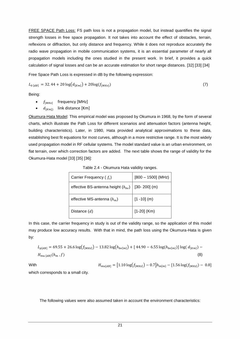
FREE SPACE Path Loss: FS path loss is not a propagation model, but instead quantifies the signal
strength losses in free space propagation. It not takes into account the effect of obstacles, terrain,
reflexions or diffraction, but only distance and frequency. While it does not reproduce accurately the
radio wave propagation in mobile communication systems, it is an essential parameter of nearly all
propagation models including the ones studied in the present work. In brief, it provides a quick
calculation of signal losses and can be an accurate estimation for short range distances. [32] [33] [34]
Free Space Path Loss is expressed in dB by the following expression:
𝐿0 [𝑑𝐵] = 32. 44 + 20 log(𝑑[𝐾𝑚]) + 20log (𝑓[𝑀𝐻𝑧]) (7)
Being:
𝑓[𝑀𝐻𝑧] frequency [MHz]
𝑑[𝐾𝑚]) link distance [Km]
Okumura-Hata Model: This empirical model was proposed by Okumura in 1968, by the form of several
charts, which illustrate the Path Loss for different scenarios and attenuation factors (antenna height,
building characteristics). Later, in 1980, Hata provided analytical approximations to these data,
establishing best fit equations for most curves, although in a more restrictive range. It is the most widely
used propagation model in RF cellular systems. The model standard value is an urban environment, on
flat terrain, over which correction factors are added. The next table shows the range of validity for the
Okumura-Hata model [33] [35] [36]:
Table 2.4 - Okumura Hata validity ranges.
Carrier Frequency ( 𝑓𝑐) [800 – 1500] (MHz)
effective BS-antenna height (ℎ𝑏𝑒) [30- 200] (m)
effective MS-antenna (ℎ𝑚) [1 -10] (m)
Distance (𝑑) [1-20] (Km)
In this case, the carrier frequency in study is out of the validity range, so the application of this model
may produce low accuracy results. With that in mind, the path loss using the Okumura-Hata is given
by:
𝐿𝑝[𝑑𝐵] = 69.55 + 26.6 log(𝑓[𝑀𝐻𝑧]) − 13.82 log(ℎ𝑏𝑒[𝑚]) + [ 44.90 − 6.55 log(ℎ𝑏𝑒[𝑚])] log ( 𝑑[𝐾𝑚]) −
𝐻𝑚𝑢 [𝑑𝐵](ℎ𝑚 , 𝑓) (8)
With 𝐻𝑚𝑢[𝑑𝐵] = [1.10 log(𝑓[𝑀𝐻𝑧]) − 0.7]ℎ𝑚[𝑚] − [1.56 log(𝑓[𝑀𝐻𝑧]) − 0.8]
which corresponds to a small city.
The following values were also assumed taken in account the environment characteristics:

22
Table 2.5 - Okumura-Hata model assumptions.
Frequency ( 𝑓 ) 2630 (MHz)
effective BS-antenna height (ℎ𝑏𝑒) 15 (m) (considering
an average 3 floor building scenario)
effective MS-antenna height (ℎ𝑚) 1.5 (m)
The COST 231 Extended HATA: this model is an extension for the Hata model, which is based in the
previous Okumura-Hata model, by COST (“COopération européenne dans le domaine de la recherche
Scientifique et Technique”), in order to cover a wider range of frequencies. COST [38] is a European
Union Forum for cooperative scientific research which has developed this model and some others based
in various experiments and researches. [33] [37]
This particular model is applicable to urban areas under the following conditions:
Table 2.6 - COST 231 Extended Hata validity ranges.
Carrier Frequency ( 𝑓𝑐) [1500 – 2000] (MHz)
BS-antenna height (ℎ𝑏𝑒) [30- 200] (m)
MS-antenna (ℎ𝑚) [1 -10] (m)
Distance (𝑑) [1-20] (Km)
When comparing with the previous model (Okumura-Hata) the major difference is the operability in
higher frequencies (1.5 to 2 GHz). Taking into account the used frequency, 2630 MHz, it could mean
more reliable results.
The model is expressed by the following equation:
𝐿𝑝 = 46.30 + 33.90 log(𝑓[𝑀𝐻𝑧]) − 13.82 log(ℎ𝑏𝑒[𝑚]) + [44.90 − 6.55 log(ℎ𝑏𝑒[𝑚])] log(𝑑[𝑘𝑚])
− 𝐻𝑚𝑢[𝑑𝐵](ℎ𝑚, 𝑓) + 𝐶𝑚[𝑑𝐵] (9)
Where 𝐶𝑚[𝑑𝐵] {0, 𝑠𝑚𝑎𝑙𝑙 𝑐𝑖𝑡𝑖𝑒𝑠
3, 𝑢𝑟𝑏𝑎𝑛 𝑐𝑒𝑛𝑡𝑒𝑟𝑠
The COST 231–Walfish–Ikegami Model: This model is a combination of J. Walfisch and F. Ikegami
model. The COST 231 project further developed this model. Now it is known as COST 231 Walfisch-
Ikegami model. It distinguishes different terrain with different proposed parameters. Also it distinguishes
between two different propagation scenarios: Line of sight (LOS) and Non-line of sight (NLOS). [33] [35]
[39]
For the first, LOS, the path loss is expressed by the following expression:

23
𝐿𝑃[𝑑𝐵] = 42.6 + 26 log(𝑑[𝐾𝑚]) + 20log (𝑓[𝑀𝐻𝑧]) (10)
For the NLOS case, this model takes into account multiple parameters, which makes the model more
complex and less suitable for generalizations. The model consists of free space path loss (seen earlier)
𝐿0, the multiscreen loss 𝐿𝑚𝑠𝑑 along the propagation path, and the attenuation from the last roof edge to
the UE, 𝐿𝑟𝑡𝑠 (roof-top-to-street diffraction and scatter loss).
𝐿𝑝[𝑑𝐵] = 𝐿𝑜 [𝑑𝐵] + 𝐿𝑚𝑠𝑑[𝑑𝐵] + 𝐿𝑟𝑡𝑠[𝑑𝐵] (11)
Figure 2.15 - Parameters in the COST 231-Walfish-Ikegami model. [35]
As the above picture illustrates, to evaluate this model one must know:
ℎ𝑟𝑜𝑜𝑓 building height
ℎ𝑏 height of the BS (Base Station)
ℎ𝑚 height of the MS (Mobile Station)
𝑤 width of the street
∆ℎ𝑚 = ℎ𝑟𝑜𝑜𝑓 − ℎ𝑚
𝑏 distance between two buildings
So, these detailed and specific parameters make the model less fitted to accomplish the objective of
this work, which consists in a more general model suitable to describe a heterogeneous and vast area.
Therefore the COST 231–Walfish–Ikegami Model will be assessed only for the LOS situations.
The CCIR Model: This empirical model was developed by the CCIR (Comité Consultatif International
des Radio-Communication, now ITU-R). It combines the effects from free-space path loss and terrain
induced path loss. [40]
This model is expressed by the following equation:
𝐿𝑝[𝑑𝐵] = 69.55 + 26.16 log(𝑓[𝑀𝐻𝑧]) − 13.82 log(ℎ𝑏) − 𝑎(ℎ𝑚) + (44.9 − 6.55 log(ℎ𝑏) log(𝑑[𝐾𝑚])) − 𝐵 (12)
Where: 𝑎(ℎ𝑚) = (1.1 log(𝑓[𝑀𝐻𝑧]) − 0.7)ℎ𝑚 − (1.56 log(𝑓[𝑀𝐻𝑧]) − 0.8)
𝐵 = 30 − 25log (% 𝑜𝑓 𝑎𝑟𝑒𝑎 𝑐𝑜𝑣𝑒𝑟𝑒𝑑 𝑏𝑦 𝑏𝑢𝑖𝑙𝑑𝑖𝑛𝑔𝑠)
Being:

24
𝑑[𝐾𝑚]) link distance [Km]
ℎ𝑏 height of the BS (Base Station) [m]
𝑓[𝑀𝐻𝑧] frequency [MHz]
ℎ𝑚 height of the MS (Mobile Station) [m]
There is no defined range validity for this model, and there were assumed the following values:
ℎ𝑏 = 15𝑚
ℎ𝑚 = 1.5𝑚
% 𝑜𝑓 𝑎𝑟𝑒𝑎 𝑐𝑜𝑣𝑒𝑟𝑒𝑑 𝑏𝑦 𝑏𝑢𝑖𝑙𝑑𝑖𝑛𝑔𝑠 = 25%
2.3.2 Performance Model
The Link Level Performance Model [30] shows that the throughput can be approximated by an
attenuated and truncated form of the Shannon bound: The Shannon bound represents the maximum
theoretical throughput that can be achieved by an AWGN (Additive White Gaussian Noise) channel for
a given SNR (Signal to Noise Ratio). In this model, the following equations estimated the throughput for
a given SNR, when using link adaptation:
𝑇ℎ𝑟𝑜𝑢𝑔ℎ𝑝𝑢𝑡, 𝑇ℎ𝑟,𝑏𝑝𝑠
𝐻𝑧= {
𝑇ℎ𝑟 = 0, 𝑓𝑜𝑟 𝑆𝑁𝐼𝑅 < 𝑆𝐼𝑁𝑅𝑀𝐼𝑁
𝑇ℎ𝑟 = 𝛼. 𝑆(𝑆𝐼𝑁𝑅), 𝑓𝑜𝑟 𝑆𝐼𝑁𝑅𝑀𝐼𝑁 < 𝑆𝐼𝑁𝑅 < 𝑆𝐼𝑁𝑅𝑀𝐴𝑋
𝑇ℎ𝑟 = 𝑇ℎ𝑟𝑚𝑎𝑥 , 𝑓𝑜𝑟 𝑆𝐼𝑁𝑅 > 𝑆𝐼𝑁𝑅𝑀𝐴𝑋
(13)
Where:
𝑆(𝑆𝐼𝑁𝑅) is the Shannon bound: 𝑆(𝑆𝐼𝑁𝑅) = log2(1 + 𝑆𝐼𝑁𝑅) 𝑏𝑝𝑠/𝐻𝑧
𝛼 attenuation factor, representing implementation losses
𝑆𝐼𝑁𝑅𝑀𝐼𝑁 Minimum SNIR of the codeset, dB
𝑇ℎ𝑟𝑚𝑎𝑥 Maximum throughput of the codeset, bps/Hz
𝑆𝐼𝑁𝑅𝑀𝐴𝑋 SNIR at which max throughput is reached S-1 (𝑇ℎ𝑟𝑚𝑎𝑥), dB
These parameters can be chosen to represent different system configurations and link conditions.
When using link adaptation, the maximum throughput of a given MCS (Modulation and Coding Scheme)
is the product of the coding rate (rate between redundant bits and data bits) and the number of bits per
modulation symbols (QPSK:2 ; 16-QAM:4 ; 64-QAM:6). Throughput has units of data bits per modulation
symbol. This is commonly normalised to a channel of unity bandwidth, which carries one symbol per
second. The units of throughput then become bits per second, per Hz.
Each MCS requires a minimum SINR to operate with acceptable low BLER (Bit Error Rate) in the output
data, so, to achieve higher throughput, higher SINR is required. The AMC (Adaptive Modulation and
Coding) is done by measuring and feeding back the channel SINR to the transmitter, which then decides
the best MCS from a codeset (which contains a number of MCSs designed to cover a range of SNR) to
maximise throughput at the present SINR.

25
Figure 2.16 - Throughput of a set of Coding and Modulation Combinations in LTE, assuming AWGN
channels. [30]
The previous figure illustrates the throughput (spectral efficiency) for different MCS in LTE. It also shows
the theoretical maximum throughput, represent by the Shannon Bound.
So, as stated before, the system performance (spectral efficiency) can be approximated by an
attenuated and truncated form of the Shannon bound:
Figure 2.17 - Approximating AMC with an Attenuated and Truncated form of the Shannon Bound. [30]
Using these principals and the gathered data, the objective is to plot and obtain an approximated curve
(which is an attenuated and truncated form of the Shannon Bound), that describes the real live
measurements performance: for the measured SINR, what is the spectral efficiency (bps/Hz).

26
Chapter 3
Drive Test
3 Introduction
This chapter will address the results obtained in the performed Drive Test. The test occurred in the city
of Castelo Branco and the collected data was provided to be studied in the present dissertation.

27
3.1 Introduction
Before specifying the results, it is relevant to emphasize the importance of performing this kind of tests
[41] [42] .A drive test provides measurements about the real conditions of the network. In particular, it
can show how the network is performing, the covered area, or the behaviour of a specific cell or cells.
The versatility of the drive test, and the real-world conditions nature, makes it one of the most useful
and accurate tools for Engineers who need to plan and enhance mobile networks.
Usually the drive test is performed using a vehicle and two measurement components: instrumented
mobile phones (test engineering phones) and measurement receivers (RF scanner). They both have
different purposes: the mobile phone gives information about the user experience of the network, and
the scanner gives a complete overview about RF reception. The gathered data is recorded to a PC and
then analysed with proper software. Also, these devices are equipped with GPS, which allows accurately
registering of the route made during the DT.
There are a wide variety of data that can be collected during these tests, since RF conditions, to
exchanged messages between the cellular phone and the BS, so it is essential to know what to measure
and understand those measurements. The following list from [42] exemplifies the kind of data collected
during a DT:
Signal intensity
Signal quality
Interference
Dropped calls
Blocked calls
Anomalous events
Call statistics
Service level statistics
QoS information
Handover information
Neighbouring cell information
GPS location co-ordinates
Also, Drive Testing can be motivated by multiple reasons, including cell optimization, network
benchmark, technology/feature testing, quality monitoring and new cell validation.
In LTE’s specific case, there are multiple measurements to be monitored and analysed, with the
following being highlighted for their importance:
RSRP (Reference Signal Received Power): measurement of the signal strength received by the
mobile phone (coverage). In the definition RSRP represents the average received power by the UE,
from the reference signal resource elements over a desired bandwidth. The RSRP is reported in the
RRC measurement reports and the reporting range is defined from -140dBm to -44dBm with 1dB
resolution. Also, and for the case of an outdoor LTE cell, three categories of values can be considered:

28
[29] [43]
RSRP> -75 dBm: excellent QoS, unless there are too many users occupying the available
bandwidth
-95>RSRP>-75 dBm: slight degradation of the QoS; Throughput will decline 30 to 50% when
RSRP goes from -75 to -95 dBm.
RSRP< -95 dBm: QoS becomes unacceptable; Throughput will decline and tend to zero at
around -100 and -108 dBm; In these conditions it is likely to occur a call drop.
RSRQ (Reference Signal Received Quality): is a measure of signal quality, which means the Signal-
to-Noise ratio. [29] The calculation of RSRQ can be obtained by the following formula:
𝑅𝑆𝑅𝑄[𝑑𝐵] = 10𝑙𝑜𝑔𝑅𝑆𝑅𝑃
𝑅𝑆𝑆𝐼3 (14)
The RSRQ range is defined from -19.5 to -3 dBm, with a 0.5 dBm resolution. Usually, if RSRP remains
stable, even if the UE is in motion, and RSRQ starts decreasing, this means that the interference is
rising. If both RSRP and RSRQ starts decreasing this means the loss of coverage. So, as seen before,
the interpretation of both RSRP and RSRQ can provide a useful representation of the network’s radio
conditions, and be used to find coverage and interference problems that affect the user experience and
QoS. Like RSRP, three categories of values can be considered:
RSRQ> -9dB: ensures a good subscriber experience
-12 dB>RSRQ> -9dB: users can experience a slight degradation of QoS, but with
acceptable user experience.
RSRQ< -13 dB: below this level it’s expected to experience significant declines in the
throughput and also call drop.
SINR (Signal-to-Noise-plus-Noise Ratio): it is also a signal quality measurement, but unlike the RSRQ
it is not defined in the 3GPP specs, being defined by UE vendors. The SINR is mostly used in wireless
communications, and is defined by the power of measured usable signals divided by the sumof the
interference power (from other interfering signals) and the power of the background noise:
𝑆𝐼𝑁𝑅𝑑𝐵 =𝑆
𝑁+𝐼 (15)
The reason to measure SINR in wireless transmissions, in opposition to SNR (Signal-to-Noise Ratio)
typical from wired communications, consists in the better quantification of the RF conditions of a wireless
environment with multiple signals present simultaneously, which results in a better relation between RF
measure and the throughput. [44] [45]
Throughput: (defined in the KPIs section with more detail) represents the volume of data transmitted
within a defined time period both in Uplink and Downlink directions. In a Drive-Test, the throughput
measured represents the performance to be expected from the network in that current position, and as
showed in the radio interface section, it depends on the previous measures. [29]
3 RSSI: measurement of all of the power contained in the applicable spectrum (1.4, 3, 5, 10, 15 or
20MHz).

29
In addition to Throughput, Latency [46] is also an essential end-user performance measure that
assesses how the network is performing and what kind of QoS can be provided. It measures the amount
of time that a packet of data takes to travel to and from the destination, back to the source (RTT: Round
Trip Time). Although, no data about latency were provided, therefore latency will not be addressed in
the DT analysis.
Position: can be represented in different formats but in either one it represents a specific position in the
planet. It is used in DT to trace the path made during the test.
3.2 Results
In the next section the plots from the various measurements collected will be presented, with the goal
to provide some visual information about the network’s conditions and performance.
In order to obtain this results, the provided data from the DT (in MS Office Excel format *.xlsx) were
loaded into MapInfo Professional (v12). Then, thematic maps were created for the plotted data over the
map of the city.
In addition, an analysis to the obtained results will be made, and e the network’s performance will be
evaluated, based in the available data.

30
3.2.1 RSRP
Figure 3.1 – RSRP.

31
3.2.2 RSRQ
Figure 3.2 – RSRQ.

32
3.2.3 SINR
Figure 3.3 – SINR.

33
3.2.4 Downlink Throughput
Figure 3.4 - Downlink Throughput.

34
3.2.5 Serving Cell (PCI)
Figure 3.5 - Serving Cell (PCI).

35
3.3 Analysis
3.3.1 Coverage
As seen in figure 3.1 (RSRP), with these 4 eNBs installed in the city, a good overall coverage is
achieved, but predominantly in its surrounding areas. Bad coverage areas, highlighted in the following
picture, are essentially caused by large distance between the UE and the Serving BS.
Figure 3.6 - Bad coverage areas.
In fact, the collected data follows the trend expressed in the next chart:
Figure 3.7- Average RSRP/Distance.
These are average values, so only an overview of the general behaviour can be evaluated. It shows
that for distances larger than 1Km from the serving BS, the average RSRP drops below the -95 dBm
which affects negatively the QoS and the Throughput. Another detected area with bad coverage, but by
different cause is the following:
-110,0
-105,0
-100,0
-95,0
-90,0
-85,0
-80,0
[ 0 ; 250] ] 250 ; 500 ] ] 500 ; 750] ] 750 ; 1000] ] 1000 ; 1500] ] 1500 ; 2000] ] 2000 ; 3500]
[dB
m]
Distance [m]
Average RSRP / Distance

36
Figure 3.8 - Bad coverage area II.
In this case, the road with bad coverage (in black colour) is relatively close to the BS, but the way its
cells are oriented (30º, 120º and 240º) does not cover that specific area. An improvement to the
coverage in this specific place can be done by reorienting one cell (24 or 32) or in alternative, add a new
sector.
Also, another bad coverage area found in the DT, but with unusual behaviour is the following:
Figure 3.9 - Bad coverage area III.
In this case, as illustrated, the low coverage area is close to two BSs but, by inspection of figure 3.5
(Serving Cell), it is found that there is no dominant cell, with different cells serving here. Therefore,
improving coverage in this specific area, by creating a dominant cell, can be achieved by up tilting cell
36, which will increase its coverage area. This must be done with caution, because it will also increase
interference with neighbour cells, namely cell 24 and cell 28. In alternative, the transmitting power can
be increased in cell 36, but possible only if the cell is not currently transmitting at the maximum power.
In this area in particular, may be relevant to assure a good LTE coverage, once it is a touristic area and
with numerous potential LTE users.
Further in this section will be analysed the throughput performance and matched with the good/bad
coverage areas.
3.3.2 Quality
To evaluate the network in terms of quality (interference), there are two main measurements to consider:
RSRQ and SINR. If in the case of RSRQ the overall results, figure 3.2 (RSRQ), are between the
acceptable values to provide a good experience to the user (larger than 12 dB). If compared with the
coverage results, some correlation can be found between the bad coverage areas and bad quality areas.

37
This is an expected behaviour since the RSRQ is calculated using the RSRP value in its formula. On
the other hand, the SINR presents worse results. The worse signal quality areas are illustrated in the
following figure:
Figure 3.10 - Bad quality areas.
In fact, when comparing with the results from the coverage analysis, it is evident the overlap of the areas
affected by both bad signal reception and bad signal quality. This reinforces the idea of lack of coverage
of these areas. To better demonstrate the mentioned situation the following picture shows the SINR for
the points where the RSRP is lower than -105 dBm:
Figure 3.11 - SINR when RSRP < -105 dBm.
The opposite situation, which means the points with very good signal reception (RSRP >-85dBm) the
results show that signal quality is mostly very good:

38
Figure 3.12 - SINR when RSRP > -85 dBm.
One main conclusion that comes from the previous results and analysis, and before entering in the
performance evaluation of the present DT, is that the current networks’ state, in terms of coverage is
not enough to assure LTE coverage to all city area, at least the one covered in the present test. However,
and taking into account the distance of some of this points to the serving BS, the frequency in use (2600
MHz), it is an expected outcome, and these areas are beyond the coverage objective for the current
network set-up. Therefore, the next part of the DT analysis will provide objective answers about the
actual performance that can be achieved by this network, being conscious that the previous results will
be reflected in the following ones.
3.3.3 Performance
To emphasize the previous idea the next charts shows how Throughput relates with RSRP and SINR:
Figure 3.13 - Throughput/ RSRP.
01000020000300004000050000600007000080000
]… ;
-1
20
]
]-1
20
; -1
15
]
]-1
15
; -1
10
]
]-1
10
; -9
0]
]-9
0 ;
-85
]
]-8
5 ;
-80
]
]-8
0 ;
-75
]
]-7
5 ;
-70
]
]-7
0 ;
-65
]
]-6
5 ;
-50
]Thro
ugh
pu
t [K
bp
s]
RSRP [dBm]
Average Throughput / RSRP

39
Figure 3.14 - Throughput/ SINR.
These charts show the relation between signal reception and quality, with the (average) throughput. As
stated in chapter 2, in radio interface section, the modulation and code rate are dependent on the radio
conditions, thus this behaviour is consistent with theoretical expectation. Also and now observing the
figure 3.4 (DL throughput) in the majority of the DT the downlink speeds are between 20-50 Mb/s (in
yellow) and between 50-70 Mb/s (in green). Reminding this is a single user scenario (without shared
resources) and these values are a bit far from the theoretical maximum, but nonetheless, represent a
large improvement from the typical throughput achieved with UMTS.
Once again, when examining the worst performing areas, a match with the previous pointed out low
coverage areas can be established. So, as anticipated in this analysis, bad signal reception, in addition
to bad quality, also leads to poor throughput performance. These results reinforce the previous idea
that, in order to obtain better results and better performance, the coverage should be extended.
Figure 3.15 - Average Throughput/ Distance.
The previous chart shows the average behaviour of throughput as the user moves away from the serving
BS. Being average values, the worst performing cases are dispersed and not noticeable, but the
influence of distance in overall performance is clear.
01000020000300004000050000600007000080000
] 3
0; 2
5]
] 2
5 ;
22
]
] 2
2 ;
21
]
] 2
1 ;
20
]
] 2
0 ;
18
]
] 1
8 ;
15
]
] 1
5 ;
12
]
] 1
2 ;
10
]
] 1
0 ;
8]
] 8
; 5
]
] 5
; 2
]
] 2
; 0
]
] 0
; -2
0]
Thro
ugh
pu
t [K
bp
s]
SINR [dB]
Throughput / SINR
30000,0
35000,0
40000,0
45000,0
50000,0
55000,0
60000,0
[ 0 ; 250] ] 250 ; 500 ] ] 500 ; 750] ] 750 ; 1000] ] 1000 ; 1500] ] 1500 ; 2000] ] 2000 ; 3500]
Thro
ugh
pu
t [K
bp
s]
Distance [m]
Average Throughput / Distance
Avg Throughput[Kbps]

40
3.3.4 Serving Area
Another main analysis to be done in a DT is the area where each cell is serving. Before implementing a
new site (or more), a coverage objective (area to be served) is defined/estimated, and then, using DT
data, one can check if that objective is being accomplished, if a cell is serving outside the planned area,
or even if the cell’s coverage area overlaps with another cell.
Ideally, this kind of study should be done by gathering data using an idle setup, with no active calls, but
it was not available for the present study.
So, the figure 3.5 (serving cell) shows where each cell is serving, identified by its PCI (Physical layer
Cell Identity). In addition, and to better distinguish between different performances, the following
chart/table shows the average serving distance for each cell:
Figure 3.16 - Average serving distance/PCI.
0,00
200,00
400,00
600,00
800,00
1000,00
1200,00
1400,00
1600,00
1800,00
2000,00
Dis
tan
ce [
m]
Average Serving Distance / PCI0
4
8
12
16
20
24
28
32
36
40
44

41
Table 3.1 - Average Serving Distance / PCI.
PCI Average Serving distance(m)
0 348.76
4 627.68
8 573.16
12 444.17
16 1107.21
20 696.94
24 516.17
28 1235.98
32 1820.85
36 275.20
40 275.33
44 414.44
These data show that, in particular cell 28 and cell 32 are serving at a very long range. This is justified
by the position of the site which contains cells 24, 28 and 32. In fact, it is located at one of the city’s
higher places (near the castle): elevation of 470m. As a consequence, these cells are serving in a far
region, and even introducing interference with the other cells placed at lower points. The most effective
way to avoid this situation is the down tilting of these two cell’s antennas. On the contrary cells 36, 40
and 44 all from the same BS, only serve at short distance and in lesser points when comparing with the
other cells, which may indicate a low transmitting power.

42
3.4 Network Optimization
To simplify, network optimization can be divided in two phases: Single site verification and RF
optimization. [47] [48]
Single site verification consists in function verification at each new site, and aims to ensure that each
site is installed properly and with the correct configuration.
RF Optimization is done after all sites in a planned area are installed and working. The optimization
aims to control pilot pollution improving the signal quality, while assuring coverage to a particular area.
Also, it could be done in order to achieve and enhance some specific KPI’s and QoS targets. The
process of optimization consists in adjustment of antenna system hardware (tilt, azimuth and height
adjustment), eNB transmit power adjustment, feature algorithms, and performance parameters
tweaking. These optimization methods are common for all mobile technologies but each standard has
its own measurement definition and specific parameters.
Regarding the Drive Test in study, the main focus is on the RF optimization since there is no data
available about the sites’ configuration.
To better summarize the DT analysis/optimization, the following table shows identified problems and
recommended actions to improve performance, in a RF optimization perspective.
Table 3.2 - RF optimization.
Problem Action
Weak Coverage: mainly when RSRP levels are low or if there is no network coverage (coverage holes). This happens when the UE received levels are below the minimum access level (RXLEV_ACCESS_MIN). Also, the signal quality is poorer. This is the main problem found in the studied area.
Analyse the EIRP (equivalent isotropically radiated power) of each sector on parameter configuration and ensure EIRPs can reach maximum values
Increase pilot power
Antenna adjustment: azimuth, beam tilt, increase height (if possible)
Use high gain antennas
Deploy new eNBs if coverage problems cannot be resolved by the previous adjustments
Lack of Dominant Cell: in this case the received level of the serving cell is similar to the levels of its neighbour cells and close to cell reselection thresholds. Received levels in these areas are usually unsatisfactory. Also SINR levels (signal quality) are unstable and low. Originates frequent handovers and service drops.
Identify the cells covering an area without dominant cells
Antenna adjustment: azimuth, beam tilt
Increase the coverage by a cell with good signal levels (by adjusting engineering parameters )
Decrease coverage of other cells to avoid additional interference
Cross Coverage: happens when one or more cells are serving in a non-planned area exceeding its coverage scope. These cells have discontinuous serving areas and usually serve in another cells planned coverage scope. Generally this occurs when the site is located at a high elevation location, and its
Antenna adjustment: azimuth, beam tilt
Beam Tilt adjustment is the most effective way to control coverage (preferentially adjusting electrical tilt)
If necessary replace antennas with large tilt antennas.

43
signal propagates farther and over other cells. This can originate situations where the UE is served by a far cell that is not configured as a neighbour of the surrounding cells, which may result in a drop call when user moves from that area. Also this usually happens with cells located at both ends of shores (particularly river shores) due to water surface reflexion.
Decrease the antenna height (for a high site)
Decrease transmit power of carriers when cell performance is not affected
Also, and to better illustrate the found problems the next figure shows examples of areas affect by each
problem:
Weak coverage:
Figure 3.17 - Weak coverage Area.
Lack of dominant cell:
Figure 3.18 - Lack of dominant cell.

44
Cross Coverage:
Figure 3.19 - Cross Coverage area (pointed by the arrows).

45
Chapter 4
Simulation
4 Introduction
Combining the studied propagation and performance models [section 2.3] with the Drive Test analysis
it is possible to create simulated scenarios and predict how the performance would be in this area when
the current network is changed/enhanced.

46
4.1 Introduction
There were many different scenarios that can be studied, so for this particular simulation the focus is a
very weak coverage area identified in the DT analysis:
Figure 4.1 – RSRP.
Figure 4.2 – RSRQ.
Figure 4.3 – SINR.
Figure 4.4 – Throughput.
The previous figures confirms that indeed this area have very weak coverage and therefore a bad
performance. In the previous section (RF Optimization), there were suggested some actions that can
improve performance when encountering weak coverage areas, namely antenna adjustment, increase
transmitted power, and ultimately deploy a new eNB. In fact for this area, to effectively increase
coverage and consequently improve performance the best solution is the addition of an eNB. On the
downside, this is also the most expansive option.
To help justifying the addition of one eNB, the following table shows the current performance in that
particular area:

47
Table 4.1 - Current (average) measurements from weak coverage area.
Average RSRP [dBm] -111.44
Average RSRQ [dB] -12.24
Average SINR [dB] 3.976
Average Throughput [Mb/s] 24.04
Average Distance to Serving BS [m] 1656.06
Also, one of the main problems in this area is mainly being served by cell 28 (78.99% of the points).
This occurs due the location of this cell, an elevated area (480m), in contrast to the area in study (395-
375m). Although it can be optimized, as addressed on chapter 3 (Drive Test), this fact highly contributes
to the poor performance and supports the need of the proposed new cell.
The common practice when choosing where to place a new site, one generally attempts to co-locate
with an existing site (already with 2G and/or 3G systems and equipment), from the same operator or a
shared solution between operators. This significantly reduces cost and allows reusing the already made
cell planning and radio equipment (for example the antennas).
Following this practice, the selected location of the simulation’s eNB is an existing non-LTE site.
Note: for simulation purposes, it is assumed that the selected site is owned by or shared with this
network’s operator.
New site location:
Latitude: 39º 48’ 59.11’’ N
Longitude: 7º 29’ 2.28’’ W
Azimuths:
o Sector 1: 30º
o Sector 2: 140º
o Sector 3: 300º
The simulation contemplates two different scenarios:
1. Frequency = 2600 MHz; Bandwidth = 20 MHz
2. Frequency= 800 MHz; Bandwidth = 10 MHz
The scenario 1 uses the same frequency/bandwidth as the other sites. In this case the propagation
model defined for this area will be better accurate once it is used in the same frequency and area, only
with a different serving cell. The main drawback in this scenario is the possible additional inter-cell
interference introduced which is not taken into account by the performance model. In this case one
assumes that the relation RSRP/SINR verified in this area remains the same, because the distance
between the new site and the existing ones is of the same order of length than the distance between
each other.

48
On the other hand, scenario 2 eliminates any additional interference by using a different LTE band:
f=800 MHz, but for the same reason, the propagation model applicability will be less precise, once it
was obtained from data with a different working frequency. In order to overcame this issue and provide
better accuracy, for this scenario one uses a propagation model containing this frequency (800 MHz)
within its validity range.
The reasons to also include a scenario with the 800 MHz frequency band are firstly because it is part of
the 3 LTE bands (800, 1800 and 2600 MHz) that currently are available in Portugal. Also, using a lower
frequency results in a lower free space path loss and therefore an increased coverage range using the
same power. The downside of using this band is that the available LTE bandwidth by Portuguese
operators for this band is half (10 MHz) of the bandwidth available for the 2600 frequency (20 MHz). As
a result, the available Resource Blocks (RBs) will also be half (section 2.1.4.) so as the maximum
throughput. So despite the throughput limitation, this scenario would provide a better coverage, without
added interference.
4.2 Simulation Models
For scenario 1, and after comparing the obtained results with each model (from section 2.3.1), the COST
231 Extended HATA proved to be the best path loss model when applied to this specific area. To
minimize the error it was added an empirical distance-depend factor, which best fits the model’s curve
to the real data points behaviour. This was done using MS Excel software.
The obtained fitted model (with the additional factor) describes this area’s radio propagation profile,
allowing the estimation of the received power by the UE (estimated RSRP). This way, it is estimated the
RSRP for the case when this area is served by the proposed new site.
For scenario 2, the same reasoning were applied but using a different model, Okumura Hata.
4.2.1 Propagation Models assessment and fitting
The following figure shows the gathered RSRP data in this area.
Figure 4.5 - Drive Test RSRP measurements.
-140-130-120-110-100
-90-80-70-60-50-40
0 500 1000 1500 2000 2500
dB
m
Distance [m]RSRP [dBm]
MS1_ServerCellRSRP
Log. trendline

49
The included red line, is done by MS Excel and shows the data points’ logarithmic trend, and it is useful
when one tries to assess how the established model matches with the DT measures.
In addition to Path Loss, to calculate the Link Budget there are multiple factors to be accounted, but can
be simplified into the following equation: [49]
𝑅𝑒𝑐𝑒𝑖𝑣𝑒𝑑 𝑃𝑜𝑤𝑒𝑟𝑑𝐵𝑚 = 𝑇𝑟𝑎𝑛𝑠𝑚𝑖𝑡𝑡𝑒𝑑 𝑃𝑜𝑤𝑒𝑟𝑑𝐵𝑚 + 𝐺𝑎𝑖𝑛𝑠𝑑𝐵 − 𝐿𝑜𝑠𝑠𝑒𝑠𝑑𝐵 (16)
Using the available data, and the following assumptions:
All cells are transmitting at the same power: 𝑇𝑥 𝑝𝑜𝑤𝑒𝑟𝐵𝑆 = 43 𝑑𝐵𝑚
MS height: 1.5m
BS height: 15m
The BS Antenna radiation pattern is described by: [30]
o 𝐴(𝜃) = −𝑚𝑖𝑛 [12 (𝜃
𝜃3𝑑𝐵)
2
, 𝐴𝑚𝑖𝑛 ] 𝑤ℎ𝑒𝑟𝑒 − 180 ≤ 𝜃 ≤ 180 º, (17)
and 𝜃3𝑑𝐵 is the 3dB beam width which corresponds to 65 degrees, and 𝐴𝑚𝑖𝑛 = 20 𝑑𝐵
is the maximum attenuation.
o BS antenna Gain: 15 dBi
o 𝐺𝐵𝑆 𝑎𝑛𝑡𝑒𝑛𝑛𝑎 = 15 − 𝐴(𝜃)
Mobile Antenna Gain: 𝐺𝑀𝑆 = 0 𝑑𝐵𝑖
The losses are represented by the Path Loss, plus the added factor
Medium-small city
Propagation Models (section 2.3.1)
o Model 1: Free space Path Loss
o Model 2: Okumura-Hata
o Model 3: The COST 231–Walfish–Ikegami Model
o Model 4: COST 231 Extended Hata
o Model 5: CCIR
The first correction done, in order to reduce error, consisted on adding the average of the difference
between each model’s RSRP estimation and the RSRP measurements. Then and to better illustrate the
assessment of the various studied propagation models, the following figures shows the comparison
between the logarithmic trendlines of each model (plus the corrective constant) and the DT data RSRP:

50
Figure 4.6- Trendlines comparison between Models and DT data RSRP [dBm] / Distance [m].
In conjunction with error analysis, this shows that the best suited models and that are being used for
this area are Model 2 and 4, respectively Okumura-Hata and Cost 231 Extended Hata. Due to the validity
ranges for both models (see section 2.3.1), namely the frequency range, it was defined that for scenario
1 will be used and further optimized the Model 4, and for scenario 2 the Model 2.
To better fit the curve of each model, it was used a different corrective factor, K. This factor is distance
dependent and was obtain by linear regression when averaging the difference between measured RSRP
and simulated RSRP, as shown by the following picture, for scenario 1-Model 4:
Figure 4.7- Corrective factor (K).
-140-130-120-110-100
-90-80-70-60-50-40-30
0 500 1000 1500 2000 2500
MODEL 1
REAL
MODEL1
-140-130-120-110-100
-90-80-70-60-50-40-30
0 500 1000 1500 2000 2500
MODEL 2
REAL
MODEL2
-140-130-120-110-100
-90-80-70-60-50-40-30
0 500 1000 1500 2000 2500
MODEL 3
REAL
MODEL3
-140-130-120-110-100
-90-80-70-60-50-40-30
0 500 1000 1500 2000 2500
MODEL 4
REAL
MODEL4
-140-130-120-110-100
-90-80-70-60-50-40-30
0 500 1000 1500 2000 2500
MODEL 5
REAL
MODEL5
y = -0.002x - 14.954-50-40-30-20-10
01020304050
0 500 1000 1500 2000 2500
K Model 4
K mod 4
Linear (K mod 4)
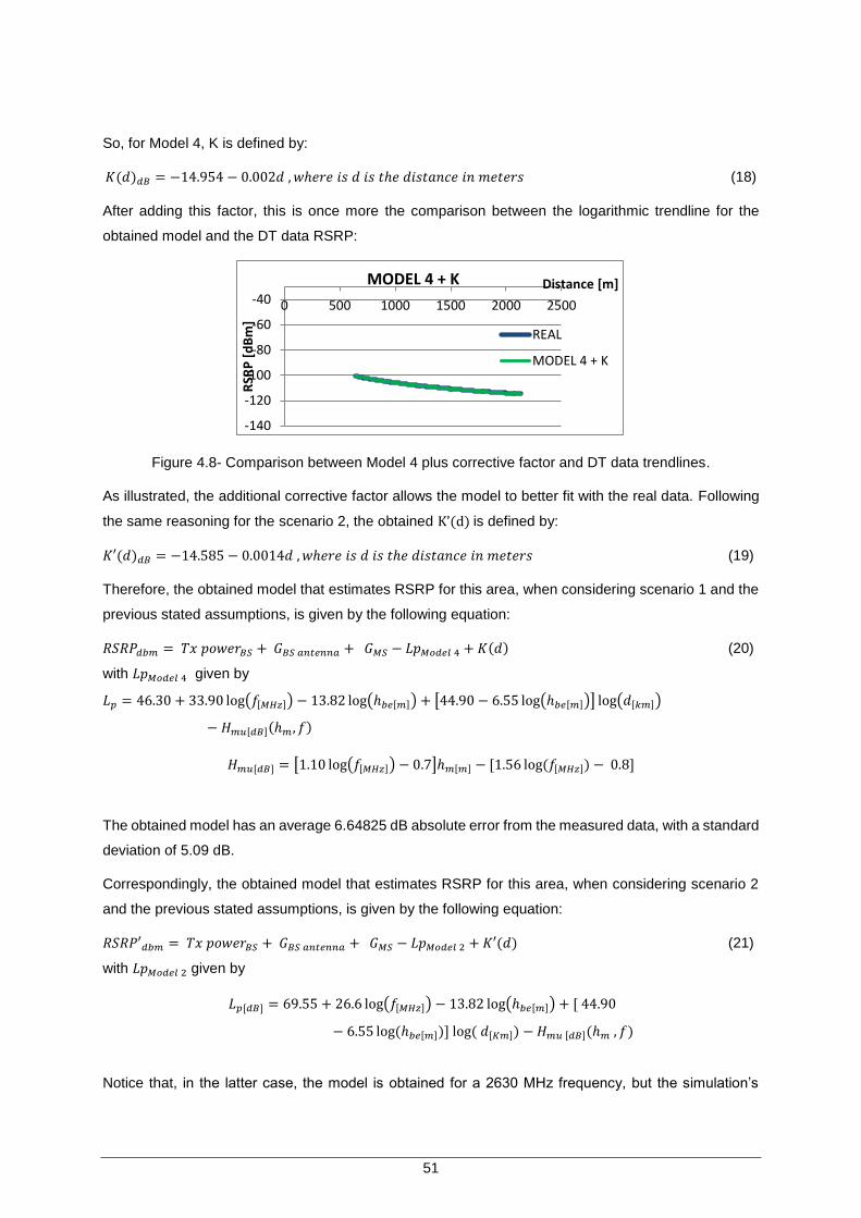
51
So, for Model 4, K is defined by:
𝐾(𝑑)𝑑𝐵 = −14.954 − 0.002𝑑 , 𝑤ℎ𝑒𝑟𝑒 𝑖𝑠 𝑑 𝑖𝑠 𝑡ℎ𝑒 𝑑𝑖𝑠𝑡𝑎𝑛𝑐𝑒 𝑖𝑛 𝑚𝑒𝑡𝑒𝑟𝑠 (18)
After adding this factor, this is once more the comparison between the logarithmic trendline for the
obtained model and the DT data RSRP:
Figure 4.8- Comparison between Model 4 plus corrective factor and DT data trendlines.
As illustrated, the additional corrective factor allows the model to better fit with the real data. Following
the same reasoning for the scenario 2, the obtained K’(d) is defined by:
𝐾′(𝑑)𝑑𝐵 = −14.585 − 0.0014𝑑 , 𝑤ℎ𝑒𝑟𝑒 𝑖𝑠 𝑑 𝑖𝑠 𝑡ℎ𝑒 𝑑𝑖𝑠𝑡𝑎𝑛𝑐𝑒 𝑖𝑛 𝑚𝑒𝑡𝑒𝑟𝑠 (19)
Therefore, the obtained model that estimates RSRP for this area, when considering scenario 1 and the
previous stated assumptions, is given by the following equation:
𝑅𝑆𝑅𝑃𝑑𝑏𝑚 = 𝑇𝑥 𝑝𝑜𝑤𝑒𝑟𝐵𝑆 + 𝐺𝐵𝑆 𝑎𝑛𝑡𝑒𝑛𝑛𝑎 + 𝐺𝑀𝑆 − 𝐿𝑝𝑀𝑜𝑑𝑒𝑙 4 + 𝐾(𝑑) (20)
with 𝐿𝑝𝑀𝑜𝑑𝑒𝑙 4 given by
𝐿𝑝 = 46.30 + 33.90 log(𝑓[𝑀𝐻𝑧]) − 13.82 log(ℎ𝑏𝑒[𝑚]) + [44.90 − 6.55 log(ℎ𝑏𝑒[𝑚])] log(𝑑[𝑘𝑚])
− 𝐻𝑚𝑢[𝑑𝐵](ℎ𝑚 , 𝑓)
𝐻𝑚𝑢[𝑑𝐵] = [1.10 log(𝑓[𝑀𝐻𝑧]) − 0.7]ℎ𝑚[𝑚] − [1.56 log(𝑓[𝑀𝐻𝑧]) − 0.8]
The obtained model has an average 6.64825 dB absolute error from the measured data, with a standard
deviation of 5.09 dB.
Correspondingly, the obtained model that estimates RSRP for this area, when considering scenario 2
and the previous stated assumptions, is given by the following equation:
𝑅𝑆𝑅𝑃′𝑑𝑏𝑚 = 𝑇𝑥 𝑝𝑜𝑤𝑒𝑟𝐵𝑆 + 𝐺𝐵𝑆 𝑎𝑛𝑡𝑒𝑛𝑛𝑎 + 𝐺𝑀𝑆 − 𝐿𝑝𝑀𝑜𝑑𝑒𝑙 2 + 𝐾′(𝑑) (21)
with 𝐿𝑝𝑀𝑜𝑑𝑒𝑙 2 given by
𝐿𝑝[𝑑𝐵] = 69.55 + 26.6 log(𝑓[𝑀𝐻𝑧]) − 13.82 log(ℎ𝑏𝑒[𝑚]) + [ 44.90
− 6.55 log(ℎ𝑏𝑒[𝑚])] log ( 𝑑[𝐾𝑚]) − 𝐻𝑚𝑢 [𝑑𝐵](ℎ𝑚 , 𝑓)
Notice that, in the latter case, the model is obtained for a 2630 MHz frequency, but the simulation’s
-140
-120
-100
-80
-60
-40 0 500 1000 1500 2000 2500
RSR
P [
dB
m]
Distance [m]MODEL 4 + K
REAL
MODEL 4 + K

52
RSRP is obtained using 800 MHz, inherent to scenario 2.
4.2.2 Performance Model assessment and fitting
The first step, and in order to get an estimation for the expected throughput, is establishing a relation
between RSRP and SINR. In other words, for a given RSRP value, what SINR value to expect. Again,
to be noted that one assumes that the interference profile obtained in the Drive Test is kept after the
new site addition. Then, with the obtained SINR and using the performance model studied in section
2.3.2 is possible to estimate the Throughput in the new conditions of both considered scenarios.
The model consist on using an Attenuated and Truncated form of the Shannon Bound, given by the
equation (13), also detailed in the section 2.3.2. The fitting process consists in finding the best suited
attenuation factor.
Once again resorting to MS Excel the following figure shows the relation between RSRP and SINR for
this area
:
Figure 4.9- SINR/RSRP relation and equation.
So, using the trendline obtained, in this case polynomial of second order, it is possible to verify that it
reproduces accurately the desired relation. So, the established empirical relation, between SINR and
RSRP, is given by:
𝑆𝐼𝑁𝑅(𝑅𝑆𝑅𝑃)𝑑𝐵 = −0.0045 × 𝑅𝑆𝑅𝑃2 − 0.3015 × 𝑅𝑆𝑅𝑃 − 26.175 (22)
The curve is set to have a theoretical maximum of 30 dB which consist in the maximum SINR measured
in this DT, for a RSRP of -50 dBm.
Then, to obtain the throughput estimation the process consisted on averaging the obtained throughput
for a given SINR, plot it against the Shannon Bound and find the best suited attenuation fact for the
model, and define the maximum throughput. The following figure illustrates the stated process,
considering a 20 MHz bandwidth:
y = -0.0045x2 - 0.3015x + 26.175-25-20-15-10
-505
101520253035
-150-130-110-90-70-50SIN
R [
dB
]
RSRP [dBm]
SINR/ RSRP
SINR
PolynomialSINR
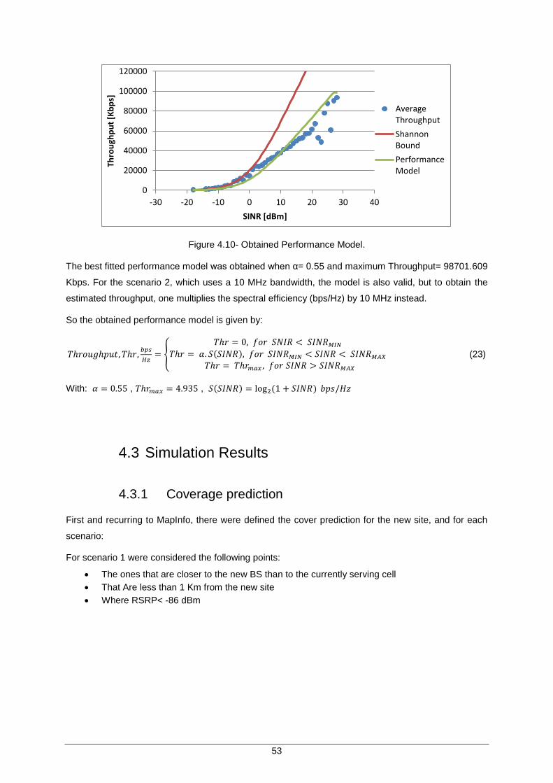
53
Figure 4.10- Obtained Performance Model.
The best fitted performance model was obtained when α= 0.55 and maximum Throughput= 98701.609
Kbps. For the scenario 2, which uses a 10 MHz bandwidth, the model is also valid, but to obtain the
estimated throughput, one multiplies the spectral efficiency (bps/Hz) by 10 MHz instead.
So the obtained performance model is given by:
𝑇ℎ𝑟𝑜𝑢𝑔ℎ𝑝𝑢𝑡, 𝑇ℎ𝑟,𝑏𝑝𝑠
𝐻𝑧= {
𝑇ℎ𝑟 = 0, 𝑓𝑜𝑟 𝑆𝑁𝐼𝑅 < 𝑆𝐼𝑁𝑅𝑀𝐼𝑁
𝑇ℎ𝑟 = 𝛼. 𝑆(𝑆𝐼𝑁𝑅), 𝑓𝑜𝑟 𝑆𝐼𝑁𝑅𝑀𝐼𝑁 < 𝑆𝐼𝑁𝑅 < 𝑆𝐼𝑁𝑅𝑀𝐴𝑋
𝑇ℎ𝑟 = 𝑇ℎ𝑟𝑚𝑎𝑥 , 𝑓𝑜𝑟 𝑆𝐼𝑁𝑅 > 𝑆𝐼𝑁𝑅𝑀𝐴𝑋
(23)
With: 𝛼 = 0.55 , 𝑇ℎ𝑟𝑚𝑎𝑥 = 4.935 , 𝑆(𝑆𝐼𝑁𝑅) = log2(1 + 𝑆𝐼𝑁𝑅) 𝑏𝑝𝑠/𝐻𝑧
4.3 Simulation Results
4.3.1 Coverage prediction
First and recurring to MapInfo, there were defined the cover prediction for the new site, and for each
scenario:
For scenario 1 were considered the following points:
The ones that are closer to the new BS than to the currently serving cell
That Are less than 1 Km from the new site
Where RSRP< -86 dBm
0
20000
40000
60000
80000
100000
120000
-30 -20 -10 0 10 20 30 40
Thro
ugh
pu
t [K
bp
s]
SINR [dBm]
AverageThroughput
ShannonBound
PerformanceModel

54
Figure 4.11- RSRP before new site (scenario 1).
The previous figure shows the location of the new site and the current RSRP on the area that predictably
would be covered by it, considering scenario 1.
This area is naturally more extensive than the one identified as weak coverage and which is studied and
modelled in the present chapter. This means that, in addition of solving the lack of LTE coverage in the
specific identified area, the new eNB will also improve the coverage/performance of all neighbouring
area, namely the red and black points from the previous figure.
For scenario 2, since it uses a lower frequency, 800 MHz, a wider area were considered. The main
reason is that, when there are 2 bands available, the usual planning practice is prioritize the usage of
the 2600 band, because it allows a higher throughput. However, due to the extended range of the 800
band, the Handover to this band is parameterized to occur when the measured RSRP levels are
considerably low.
So For scenario 2 were considered the following points:
That Are less than 1.5 Km from the new site
Where RSRP< -105 dBm
Figure 4.12 - RSRP before new site (scenario 2).
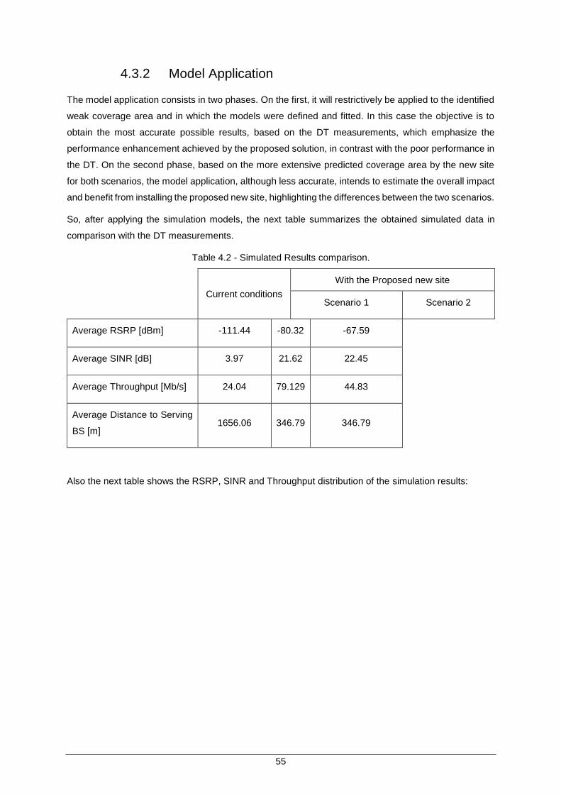
55
4.3.2 Model Application
The model application consists in two phases. On the first, it will restrictively be applied to the identified
weak coverage area and in which the models were defined and fitted. In this case the objective is to
obtain the most accurate possible results, based on the DT measurements, which emphasize the
performance enhancement achieved by the proposed solution, in contrast with the poor performance in
the DT. On the second phase, based on the more extensive predicted coverage area by the new site
for both scenarios, the model application, although less accurate, intends to estimate the overall impact
and benefit from installing the proposed new site, highlighting the differences between the two scenarios.
So, after applying the simulation models, the next table summarizes the obtained simulated data in
comparison with the DT measurements.
Table 4.2 - Simulated Results comparison.
Current conditions
With the Proposed new site
Scenario 1 Scenario 2
Average RSRP [dBm] -111.44 -80.32 -67.59
Average SINR [dB] 3.97 21.62 22.45
Average Throughput [Mb/s] 24.04 79.129 44.83
Average Distance to Serving
BS [m] 1656.06 346.79 346.79
Also the next table shows the RSRP, SINR and Throughput distribution of the simulation results:

56
Table 4.3- Simulation Results (percentage).
scenario 1 scenario 2
RSRP [dBm]
>-85 61% 99%
]-85, -95] 38% 1%
]-95, -105] 1% 0%
SINR [dB]
>20 75% 94%
]20, 14] 25% 6%
]14, 6] ~0% 0%
Throughput [Mb/s]
> 75 68% 0%
]75, 50] 32% 0%
]20, 50] 0% 100%
When comparing with the previous measurements the main conclusion to take and as expected, the
new site will allow a major performance enhancement in this specific area, and actually allow LTE
coverage with very good QoS for this area. When comparing between the two simulated scenarios, both
show advantages and drawbacks, which can be summarized as a trade-off between a wider coverage
range with better signal reception and providing higher throughput to a closer area.
Finally, the following figures show the plots corresponding to the predicted coverage area for both
scenarios:

57
Scenario 1:
Figure 4.13- Simulation: RSRP scenario 1.
Figure 4.14- Simulation: SINR scenario 1.
Figure 4.15 – Simulation: Throughput scenario 1.

58
Scenario 2:
Figure 4.16 – Simulation: RSRP scenario 2.
Figure 4.17 - Simulation: SINR scenario 2.
Figure 4.18 – Simulation: Throughput scenario 2.

59
Chapter 5
Conclusions
5 Conclusions
This chapter will contain the final considerations, regarding the obtained results. Also, it summarizes the work and studies carried out along the present dissertation.

60
LTE represents a big step forward in mobile systems. It introduced a new simplified all-IP architecture
both in access and core, leaving the traditional circuit switching present in the previous generations.
Also, it uses OFDMA for multiple access technique and MIMO for multiple antenna technique, but the
main evolution, which is highlighted in its name, comes from the considerably higher data rates and
lower latency provided.
Drive testing constitutes an essential tool to assess network conditions and performance, and the
analysis of the measured data can provide answers that help solving the identified problems and which
actions should be implemented.
Following this premise, firstly, a comprehensive DT analysis was made, focusing on identifying the areas
with poor performance. Then, taking in consideration factors, such as terrain’s orography, eNB location
and zone kind, the aim was finding the cause for that poor performance and how it could be improved.
This analysis was mostly based on the map plotting of the gathered data.
In addition, a summary of the identified problems/actions were made. These suggested actions
represent the preferential and more prioritized optimizations that are performed, especially if they can
be done remotely. Optimization also signifies finding the best solution at the lower expense possible.
To complement the Drive Test analysis, it was also studied the main KPIs (key performance indicators)
for LTE. The KPIs allow an objective evaluation and monitoring of the networks’ conditions. They are
categorized in: Accessibility, Throughput, Mobility, Retainability and Latency.
The final chapter consisted in the simulation of two scenarios, in which a new site was added to an area
with very weak LTE coverage. As mentioned, the addition of a new site (and radio components in
general) is not the first optimization action to be taken, but it is the most efficient. So, it was important to
justify the actual need for adding a new site in that specific area and show the improvement achieved.
In order to optimize the cost of this solution, one chose a location containing an existing non-LTE site.
This allows significantly reduce costs, and follows the common practise when implementing a new LTE
site.
The simulation required the usage of Propagation Models and Performance Models, in order to obtain
the estimated measures. So, these models were also studied and then evaluated against the DT data.
This study allowed the establishment of a model better suited for each considered scenario.
In addition, and to better fit the theoretical models to the real data one resorted to the MS Excel’s
“trendline” functions that helped in the curve fitting process. The obtained model that estimates the
received power (RSRP) had an average 6.64825 dB absolute error from the measured data, with a
standard deviation of 5.09 dB.
The study of how using different bands would affect performance motivated the two different scenarios.
In one of them, the frequency (2600 MHz) used were the same of the other eNodeBs, and in the other
were studied the usage of a different frequency (800 MHz) band, from the ones available in Portugal.
This means a lower frequency, with better free space propagation and without adding additional

61
interference. On the downside, this frequency band only has available half of the bandwidth (10 MHz)
in comparison to the 2600 band (20 MHz), so in consequence it only allows half of the maximum
throughput.
The simulation showed, as expected, that the performance in that area were considerably improved, but
more important than that, it showed that in order to provide LTE coverage to this kind of areas, it is a
required action. Otherwise, the low reception levels would cause the UE to reselect to 2G or 3G.
From both scenarios, the conclusion to be drawn is that depending on which factor is prioritised, between
coverage and throughput, one scenario will fit better than the other. Using the 2600 MHz band provided
an overall better performance/throughput (79.129 Mbs on average) due to its higher available
bandwidth, but to a more confined area. On the other hand, the 800 MHz frequency provides an
acceptable throughput (44.83 Mbs on average) to an extended area, improving also other nearby low
coverage areas detected. So, it was evident the impact of using different LTE bands, and their respective
benefits/disadvantages.
To conclude, the present dissertation attained the proposed objective of defining strategies for the
performance enhancement for a given LTE network. It was realised through Drive Test analysis and the
proposed strategies contemplate actions that can be applied to the existing network’s configuration and
also for an alternative scenario, in which, it was simulated and studied the addition of an eNB. This study
allowed the definition of propagation and performance models that intend to replicate the real
measurements’ behaviour and can be applied in areas with similar conditions and environment.

62

63
References
References
[1] Ericsson. Traffic and Market Data Report, June 2013
[2] GSM [Online] http://en.wikipedia.org/wiki/GSM
[3] H. Holma e A. Toskala. “LTE for UMTS – OFDMA and SC-FDMA Based Radio Access”, John
Wiley & Sons, Ltd, April 2009
[4] UMTS [Online] http://en.wikipedia.org/wiki/UMTS
[5] Erik Dahlman, Stefan Parkvall, Johan Sköld, Per Beming, "3G Evolution – HSPA and LTE for
Mobile Broadband", 2nd edition, Academic Press, 2008
[6] H. Holma e A. Toskala. “WCDMA for UMTS: HSPA Evolution and LTE, 4th Edition”, John Wiley &
Sons, Ltd, September 2007
[7] Mobile Network Evolution and the LTE Architecture [Online]
http://www.wirelessweek.com/articles/2010/10/part-2-mobile-network-evolution-and-lte-architecture
[8] Alcatel Lucent. “The LTE Network Architecture – Strategic White Paper”. White Paper
[9] 3GPP [Online] http://www.3gpp.org/technologies/keywords-acronyms/100-the-evolved-packet-core
[10] Long Term Evolution (LTE) & Ultra-Mobile Broadband (UMB) Technologies for Broadband Wireless
Access [Online] http://www.cs.wustl.edu/~jain/cse574-08/ftp/lte/
[11] Orthogonal frequency-division multiple access [Online]
http://en.wikipedia.org/wiki/Orthogonal_frequency-division_multiple_access
[12] Ericsson “Long Term Evolution (LTE): an introduction”, October 2007
[13] Agilent Technologies “3GPP LTE: Introducing Single-Carrier FDMA” January 2008
[14] Liang Zhang “Network Capacity, Coverage Estimation and Frequency Planning of 3GPP Long
Term Evolution”, Master thesis, September 2009
[15] [Online] http://commons.wikimedia.org/wiki/File:Modul.jpg
[16] Stefania Sesia, Issam Toufik, Matthew Baker “LTE - The UMTS Long Term Evolution: From
Theory to Practice, 2nd Edition” July 2011
[17] MIMO [Online] http://en.wikipedia.org/wiki/MIMO
[18] How Many Various Gains brought by the MIMO for LTE [Online] http://www.teletopix.org/4g-lte/how-
many-various-gains-brought-by-the-mimo-for-lte/

64
[19] What is MIMO? Multiple Input Multiple Output Tutorial [Online]
http://www.radio-electronics.com/info/antennas/mimo/multiple-input-multiple-output-technology-
tutorial.php
[20] Rhode & Schwarz “LTE Transmission Modes and Beamforming”, white paper, October 2011
[21] Telesystem Innovations “LTE in a Nutshell: The Physical Layer”, 2010
[22] An overview of the LTE physical layer [Online]
http://www.eetimes.com/document.asp?doc_id=1278096&page_number=2
[23] F. Rezaei, M. Hempel, H. Sharif “LTE PHY Performance Analysis under strict 3GPP parameter”,
submitted to Vehicular Technology Conference (VTC), September 2010
[24] Interoperability between LTE FDD/TDD network [Online]
http://blog.3g4g.co.uk/2011/11/interoperability-between-lte-fddtdd.html
[25] Maria Djanatliev “LTE TDD Technology Overview” [Online]
http://www.slideshare.net/GoingLTE/lte-tdd-technology-overview
[26] Ralf Kreher, Karsten Gaenger “LTE Signaling: Troubleshooting and Optimization”, John Wiley &
Sons, Ltd, December 2010
[27] How and Which KPI to Check before and after LTE Launch [Online] http://www.teletopix.org/4g-
lte/how-and-which-kpi-to-check-before-and-after-lte-launch/
[28] LTE KPI Measurement Methodology and Acceptance Procedure [Online]
http://www.teletopix.org/4g-lte/lte-kpi-measurement-methodology-and-acceptance-procedure/
[29] 3GPP, TS 32.450 V10.1.0, “Key Performance Indicators (KPI) for
Evolved Universal Terrestrial Radio Access Network (E-UTRAN): Definitions (Release 10)”, June 2011
[30] 3GPP, TR 136 942 V11.0.0, “LTE; Evolved Universal Terrestrial Radio Access (E-UTRA); Radio
Frequency (RF) system scenarios” [Annex A] October 2012
[31] Castelo Branco [Online], http://portugalfotografiaaerea.blogspot.pt/2012/12/castelo-branco.html
[32] Free-space path loss [Online] http://en.wikipedia.org/wiki/Free-space_path_loss
[33] L. Correia “Mobile system communications: Propagation Models chapter”, Sistemas de
Comunicações Móveis classes 2013
[34] Path Loss: Models of "large-scale effects" [Online]
http://people.seas.harvard.edu/~jones/es151/prop_models/propagation.html#propmain
[35] Andreas F. Molisch “Wireless Communications”, [Appendix 7.A] John Wiley & Sons, Ltd, Second
Edition, November 2010
[36] Hata-Okumura Model [Online] http://www.awe-communications.com/Propagation/Rural/HO/
[37] COST Hata model [Online] http://en.wikipedia.org/wiki/COST_Hata_model
[38] European Cooperation in Science and Technology [Online] http://en.wikipedia.org/wiki/COST

65
[39] Didarul Alam Rezaul Huque Khan, “Comparative Study of Path Loss Models of WiMAX at 2.5
GHz Frequency Band”, April 2013, International Journal of Future Generation Communication and
Networking
[40] Hata and CCIR Formulas [Online] http://www.antd.nist.gov/wctg/manet/calcmodels_dstlr.pdf
[41] JDSU “Drive Testing LTE”, white paper February 2012
[42] Drive testing [Online] http://en.wikipedia.org/wiki/Drive_testing
[43] LTE Measurements – RSRP [Online Video]
http://lteuniversity.com/get_trained/video_tutorials/m/videotutorials/11523.aspx
[44] Signal-to-interference-plus-noise ratio [Online] http://en.wikipedia.org/wiki/Signal-to-interference-
plus-noise_ratio
[45] LTE RF conditions classification [Online] http://radioaccess.blogspot.pt/2012/11/lte-rf-conditions-
classification.html
[46] NSN “Latency The impact of latency on application performance”, White Paper, July 2007
[47] Huawei Confidential document
[48] LTE RF Planning [Online] https://sites.google.com/site/lteencyclopedia/lte-radio-link-budgeting-
and-rf-planning/lte-rf-planning
[49] Link Budget [Online] http://en.wikipedia.org/wiki/Link_budget