Embed Size (px)
Citation preview
Performance Evaluation Methods to Study IEEE 802.11 Broadband Wireless Networks under the PCF Mode 509
Performance Evaluation Methods to Study IEEE 802.11 Broadband Wireless Networks under the PCF Mode
Vladimir Vishnevsky and Olga Semenova
0
Performance Evaluation Methods to StudyIEEE 802.11 Broadband Wireless Networks
under the PCF Mode
Vladimir Vishnevsky and Olga SemenovaZAO Research & Development Company "Information and Networking Technologies"
Russia
1. Introduction
In the Chapter, we consider design concepts and protocols for metropolitan area wireless net-works, realization methods for adaptive dynamic polling in these networks and investigationof their main performance characteristics by means of stochastic polling models.Polling mechanism is widely used in the wireless metropolitan area networks (WMANs). Inthe wireless networks with PCF (Point Coordination Function), a base station polls subscriberstations accordingly to a polling table describing the order of polling. For IEEE 802.11 Wi-Finetworks, the polling is an option; for WiMAX networks (IEEE 802.16), it is basic. Using thePCF in the MANs allows to avoid the problem of hidden stations, efficiently schedule an orderof station access to the wireless channel, flexibly control the radio cell operation and changeits parameters correspondingly to the current situation by adjusting only the base station.The methods to form and keep up the polling table are not specified in the standard thus thewireless network developers can freely decide on how to realize it. The specific polling mech-anism and its parameters are the main factors determining the efficiency of the broadbandwireless MAN with centralized control. In the Section, we give the description of the IEEE802.11 protocols and the main directions of their development, including the recent versionsIEEE 802.11n and IEEE 802.11 VHT. The much attention is given to development and mod-elling of the algorithms to poll subscriber stations, the schemes of adaptive dynamic polling(ADP). The adaptive dynamic polling is proposed to cut down the expenses of polling theempty subscriber stations and stations that stopped working for some reason. The adaptivedynamic polling is the prospective direction of developing the IEEE 802.11 broadband wirelessnetworks.We present the models of adaptive polling system and the system with threshold polling. Withthe adaptive polling order, the order of queue visit is cyclic but a server does not visit queuesthat were empty at the instant of polling in the previous cycle. Under the threshold polling,a queue is served only of its length exceeds the given threshold. Such service discipline is apossible way to assign a priority to a queue depending on the threshold value, and it allowsserver to give more attention to queues with high traffic intensity rather than spend time inqueues with low traffic.
24
www.intechopen.com
Trends in Telecommunications Technologies510
2. Performance evaluation of the broadband wireless networks
Polling mechanism is widely used in the metropolitan area wireless transmission networks. Inthe wireless networks with PCF (Point Coordination Function), a base station polls subscriberstations accordingly to a polling table describing the order of polling. For IEEE 802.11 Wi-Finetworks, the polling is an option; for WiMAX networks (IEEE 802.16), it is basic. In thisSection, we consider design concepts and protocols for metropolitan area wireless networks,realization methods for adaptive dynamic polling in these networks.
2.1 Development of the broadband wireless networks: state of the art and prospects
In the recent years, the wireless transmission networks become the main direction of thenetwork industry development. It was provided by both the rapid Internet developmentand the adoption of new progressive methods for coding, modulation and wireless datatransmission. Recently, it is obvious that broadband wireless networks are without a rivalwith their efficiency of deployment, portability, price and area of potential applications.Wireless technologies displace the wired one almost in all places where they can providehigh-quality data transmission. The tendency is evidently continuing to the future since thewireless world is more comfortable. Nowadays, the wireless data transmission technologieshave become ingrained in everyday life of millions of people and enterprises. The modernwireless networks allows solving variety of problems from the indoor network managementto the distributed wireless networks within a city, a region or a country. Low cost, efficiency ofdeployment, wide performance capabilities to transmit data, IP telephony and video streams,all these make the wireless technologies the most rapidly developing telecommunication area.Rapid growth of the broadband wireless networks often called the "wireless revolution" in thefield of data transmission networks is explained by a number of their own distinctive features,such as
– flexibility of a network topology enabling the dynamic change of the topology withouttime loss when mobile users connect to the network, move or disconnect;
– high data transmission rate (up to 54 Mbit/sec);
– rapidity of designing and realization which is significant because of the strict technicalconditions to network construction;
– high unauthorized access protection level;
– high-priced laying or rent of the fiber optic or copper cable are not needed.
Recently, the wireless technologies provide effective solution of the following problems:
– mobile access to the Internet;
– organization of the wireless radiocommunication between workstations of a local areanetwork (organization of the wireless access to a local area network resources);
– unification of local area networks and workstations into a single data transmissionnetwork and providing the remote access to the Internet for local area networks;
– last mile problem solution;
– interconnecting the automatic telephone systems with wireless channels of up to 54Mbit/sec rate;
– creation of the land cellular radio modem data networks.
www.intechopen.com
Performance Evaluation Methods to Study IEEE 802.11 Broadband Wireless Networks under the PCF Mode 511
The mentioned features of the wireless technologies are substantially brought about by the factthat wireless networks operating within the range 2.4-6.4 GHz are based on the technology ofbroadband, or noise-type signal. The technology was initially used for the military purposesand recently it is efficiently used for civil radio networks.The broadband wireless technologies use two radically different methods of frequency bandutilization, they are Direct Sequence Spread Spectrum (DSSS) and Frequency Hopping SpreadSpectrum (FHSS). Both methods imply the frequency band division into n subchannels. UnderDSSS method, each data bit is coded as a sequence of n bits, and all those n bits are transmittedsimultaneously through all n subchannels, and the coding algorithm is individual for each pair’transmitter-receiver’ so as to provide the transmission security. Under the FHSS method, astation transmits only through one of n subchannels at each time moment periodically changingthe subchannel. Those change-overs (hops) happen simultaneously for both a transmitter anda receiver, and their sequence is pseudo-random and is known only for ’transmitter-receiver’pair that provide the transmission security as well.Undoubtedly, each method has its own advantages and disadvantages. The DSSS methodallows reaching the maximal throughput and due to the n-modular redundancy it, first, pro-vides the narrow-band interference immunity, and, second, gives the opportunity to use thelow power signal so as not to interfere with ordinary radio devises. On the other hand, theFHSS equipment is considerably simpler and cheaper and has the broadband interferenceimmunity.To work with the wireless networks, we need the special MAC (Media Access Control) proto-cols due to the fundamental differences from the cable medium, namely the lack of completeconnection (the stations can be hidden from each other), the wireless medium is not protectedfrom the outside signals and its signal propagation properties are asymmetric and variable bytimes. In order to provide the effective wireless medium access, the international standards,protocols and recommendations are developed which specify the physical and MAC layers ofwireless networks: Bluetooth, ETSI Hiperlan and IEEE 802.11 for local area networks (LAN);IEEE 802.11 using the necessary amplifiers and parabolic antennae for metropolitan area net-works (MAN), and finally, IEEE 802.16 and callular telephony technologies modified for dataand video images transmission (GPRS, UMTS and CDMA-2000) for MANs (Vishnevsky et al.,2009).Among the LAN and MAN developers, the IEEE 802.11 protocol is very popular (referred to asRadio-Ethernet as well) adopted as an international standard in 1997 and having the followingfeatures:
• it can be used in both LANs and MANs;
• both DSSS and FHSS methods of the broadband wireless network deployment areregulated;
• the huge number of software and hardware of the large companies (such as CISCOAironet, Lucent Technologies, Alvarion, etc.) in the world markets support the standard.
The IEEE 802.11 protocol determines two network development topology, they are topologieswith infrastructure and so called ad-hoc-topology. With infrastructure topology, a wirelessnetwork has a single access point (or base station). An access point provides the synchroniza-tion and coordination for stations within the range, transmits broadcast packets and, what isof the great importance, can be a portal into the global network. Such topology is referred toas the Basic Service Set (BSS). To cover the wide area, it is possible to set up several accesspoints working in different frequency channels and connected to the joint wired or wireless
www.intechopen.com
Trends in Telecommunications Technologies512
backbone. Besides, the subscriber stations can be provided with a roaming between the accesspoints. Such topology is called the Extended Service Set (ESS). The ad-hoc topology calledthe Independent Basic Service Set (IBSS) is the network performance scheme under which thenumerous stations are connected directly avoiding connection to the special access point. Thisregime is effective when the wireless network infrastructure is not constructed (e.g., conferencehall), or can not be constructed by some reason.The IEEE 802.11 protocol specifies the data transmission rate equal to 1 or 3 Mbit/sec, with thisthe packet header and the service information can be transmitted at 1 Mbit/sec. Note that thetransmission rate did not satisfy the users even when the protocol was adopted and approved.In order to make the wireless technology popular, cheap and, above all, to satisfy the modernstrict conditions of business applications, the developers had to set up new standards whichwere the extensions of IEEE 802.11. Consider them in brief.IEEE 802.1a. The IEEE 802.11a protocol exploits the radio frequency band of 5 GHz (5150-5250MHz, 5250-5350 MHz and 5725-5850 MHz). In contrast to IEEE 802.11, the protocol appliesnot the spectrum broadening technologies but Orthogonal Frequency Division Multiplexing(OFDM), also referred to as multiple carrier modulation, which uses several carrier signals ofdifferent frequencies each transmitting a number of bites. This technology allows reaching thefollowing data transmission rates: 6, 9, 12, 18, 24, 36, 48 and 54 Mbit/sec.IEEE 802.11b. The IEEE 802.11b protocol involves the changes within the IEEE 802.11 physicallayer. The network operates in 2.4 GHz radio frequency band. But the other signal modulationtechnology, Complementary Code Keying (CCK) allows reaching the rates 5.5 and 11 Mbit/secand increases the connection stability in interference and multipath signal propagation condi-tions.IEEE 802.11g. The IEEE 802.11g protocol as long as IEEE 802.11b operates in 2,4 GHz radiofrequency band but applies the orthogonal frequency division multiplexing (OFDM) allowingto reach the data transmission rate equivalent to IEEE 802.11a (up to 54 Mbit/sec). Nevertheless,the protocol enables stations to get back to rates 1, 2, 5.5 and 11 Mbit/sec, i.e to CCK modulation.Therefore, the devices 802.11b and 802.11g are compatible within a segment of broadbandwireless network.Recently, the standard IEEE 802.11n describing the networks with data transmission rate100Mbit/sec on the base of antenna system technology MIMO is going to be finished. Themobile version of the standard (IEEE 802.11p) and the addition IEEE 802.11e to provide theguaranteed quality of service (QoS).In 2007, the generalized standard (see IEEE Std. 802.11-2007) was approved involving all stan-dards finished before June, 2007. They are IEEE 802.11a/b/g mentioned above and additionsIEEE802.11e/h/i/j.The standard IEEE 802.11 is constantly being improved and developed to provide new cus-tomer services and to increase the data transmission rate and its quality. In 2009, it is plannedto release a number of new standards being developed from 2003-2004. First of all, they areIEEE 802.11n and IEEE 802.11s. Though those standards are being finished, many companieshave started production of devices and provide the wireless network operation based on thedraft versions of those standards.The other standards to be approved in 2009 are:
• standard IEEE 802.11u describing communications between IEEE 802.11 networks andouter networks;
• standard IEEE 802.11r regulating procedures of switching between subscriber stationsfor delay sensible applications like IP-telephony, etc.;
www.intechopen.com
Performance Evaluation Methods to Study IEEE 802.11 Broadband Wireless Networks under the PCF Mode 513
• standard IEEE 802.11p for operation in dynamic environment, and for fast movingwireless devices, in particular;
• standard IEEE 802.11v describing the wireless network control protocols;
• standard IEEE 802.11w regulating the methods to protect supervisory frames in a wire-less network;
• standard IEEE802.11z describing the protocol for direct data exchanging between sta-tions without using an access point.
The standard IEEE 802.11k should be also mentioned but it is not included into the generalizedstandard IEEE 802.11-2007 since its final version was released at the end of 2007 only. The stan-dard regulates the mechanisms to exchange information about radio resource, radiochannelperformance and load, noise level, etc.The persistent growth of the transmission data volume, release of new applications, e.g. highdefinition video, impose heavy demands on wireless network throughput.In spite of high data transmission rate in third generation mobile networks based on LTEtechnology and in networks IEEE 802.11n (up to 300 Mbit/sec), work on new technologiescreation in the framework of IEEE 802.11 is continued. From 2007, the standard IEEE 802.11VNT (Very High Troughput) has been started providing a base for very high throughput localwireless networks with nominal speed up to 500Mbit/sec within the frequency range 6 GHz.The standard is planned to be finished in 2012.High network throughput is obtained by the MIMO technology application with 8 spacedantennas on both transmitting and receiving sides, by band enhancement up to 80 MHzthrough multiplexing of four channels of width 20 MGz, also by using OFDMA to organizefrequency division multiple access as in IEEE 802.16. The developed standard supportscompatibility with devices working under IEEE 802.11a/b/g/n.In Russian Federation, the new technology and both hardware and software for very highthroughput mesh-networks operating in the frequency range 60GHz (Vishnevsky & Frolov,2009). As compared to existing mesh-networks, the proposed approach provides transmissionrate up to 1000 Mbit/sec and makes the frequency planning and operating in duplex modeunnecessary.In the 802.11 protocol, the fundamental mechanism to access the medium is called DistributedCoordination Function (DCF). This is a random access scheme, based on the Carrier SenseMultiple Access with Collision Avoidance (CSMA/CA) protocol. Retransmission of collidedpackets for each station is managed according to binary exponential backoff rules (Section 2.2).The alternative access mechanism as an option specified in IEEE 802.11 is point coordinationfunction (PCF) under which the coordinator station manages the centralized polling of otherstations (Section 2.3).
2.2 Medium access layer in IEEE 802.11. Distributed Coordination Function (DCF)
The IEEE 802.11 protocol is the part of IEEE 802 protocols for local area networks (LANs)andmetropolitan area networks (MANs) involving the well-known protocols IEEE 802.3 (EthernetLAN) and IEEE 802.5 (Token Ring LAN). The majority of IEEE 802 protocols determines thephysical and data link layers of the Open Systems Interconnection (OSI) seven-level referencemodel of the International Organization for Standardization (ISO). Furthermore, the datalink layer is represented as two sub-layers, the Logical Link Control (LLC) and MediumAccess Control (MAC). Such division is conditioned by the fact that under the same LLC,the mechanisms providing MAC can be different. The IEEE 802.11 involves the functional
www.intechopen.com
Trends in Telecommunications Technologies514
description of both MAC and PHY layers. Both layers possess significant features, e.g. thehigh packet loss rate due to noise and collisions, and the fact that wireless data transmissioncan suffer from the unauthorized access. Logical link control is not considered in the protocolsince it is the same as in IEEE 802.2.All questions on regulation of the wireless medium sharing by the network stations are de-termined on MAC-layer. The necessity of such regulation rules is quite obvious. Imaginethe situation when each station of the wireless network sends data to the medium withoutobserving any rules. As a result of such signals interference, the destination stations cannot receive the data, and even understand the data were destined for them. Therefore, thestringent regulating rules are essential to determine the wireless medium multiple access. Themultiple access rules can be compared to the rules of the road which regulate the road sharingby road users.As it is mentioned above, there are four types of IEEE 802.11 MAC layer multiple access towireless medium, they are Distributed Coordination Function (DCF), its extension ExtendedDCF (EDCF), Point Coordination Function (PCF) and Hybrid Coordination Function (HCF).Below, we consider these mechanisms in details.The DCF is a method to organize peer-to-peer access to the wireless medium. The functionis based on the Carrier Sense Multiple Access/Collision Avoidance (CSMA/CA). With thisaccess, each station before sending a packet listens to the medium trying to detect the carriersignal and starts transmission only when the channel is idle. But in this case the probabilitythat a packet collides with another one upon its transmission is high enough, when two ormore stations find out the channel is idle and start transmission at the moment when somestation is transmitting. In order to decrease the collision probability, the Collision Avoidance(CA) mechanism is applied. The mechanism is described as follows. A station detecting thechannel idle waits for the prespecified time interval before it starts transmission. The timeinterval is random given by two intervals: the Distributed InterFrame Space (DIFS) and therandom Backoff time. Consequently, each station waits for a random time before starting datatransmission that essentially decreases the collision probability since the probability that atleast two stations have the same backoff is negligible.MAC-layer of the IEEE 802.11 protocol, its modification described in IEEE 802.11e thereof,specifies five types of a time interval between consecutive data transmissions, namely Inter-frame Space (IFS). The shortest one is SIFS (Short Interframe Space) used for special sequenceof data exchange, e.g. ACK transmission to acknowledge a frame successful reception. TheSIFS duration is specified by physical layer to give enough time for the system to switch fromreception to transmission or inversely. The other intervals are given in duration increasingorder: PIFS, used by stations with Point Coordination Function; DIFS, used by stations withDistributed Coordination Function; AIFS, used in Extended DCF (EDCF), and EIFS (ExtendedInterframe Space), used by stations after transmission error.In order to provide stations with the equal access to the channel, it is necessary to determinethe appropriate algorithm to choose the backoff time which is a number of basic time intervalscalled time-slots. To choose the random backoff, each station determines the ContentionWindow (CW) which is the range the backoff time is chosen from. The minimal CW is 31 timeslots, and maximal one is 1023 time slots. The backoff is determined as:
Backo f f = Random(CW) · SlotTime,
www.intechopen.com
Performance Evaluation Methods to Study IEEE 802.11 Broadband Wireless Networks under the PCF Mode 515
where Random(CW) is an integer uniformly chosen in the range (0, CW − 1). At each time, thevalue CW depends on the number n of the attempts failed to send a packet and is given by
CW = CW02n,
where CW0 is the minimal contention window, 0 ≤ n ≤ m, and m is the maximal number ofattempts allowed to send a packet. If the m + 1-th attempt is failed the packet is discarded.When a station tries to get an access to the channel, after the DIFS expires the backoff starts tocount down. If the channel is idle during DIFS and the backoff, the station immediately startstransmission as the backoff counter reaches 0.After the successful packet transmission, the CW is determined anew. If another stationtransmits during the backoff time, the backoff counter is frozen until the channel becomes idle(transmission is finished and DIFS expired). With this procedure, it is easy so see that the moretimes the station freezes its backoff counter the grater the probability that the packet waitingfor transmission will not collide.The described algorithm to get an access to the wireless medium guarantees the equal accessfor all stations in the network. But under such procedure, the probability of collision (thatan arbitrary packet collides upon its transmission) is still non-zero. The collision probabilitycould be reduced by extension of the maximal CW. But it leads to the grater backoff valuewhich decreases the channel throughput. Therefore, the DCF uses the following algorithmto minimize collisions. After each successful frame reception, the destination station sendsthe ACK (ACKnowledgement) after SIFS to acknowledge the transmission was successful. Ifcollision happens upon transmission the sender station does not get an ACK, so it finds outthe transmission failed. The sender waits for ACK during EIFS, and if the ACK is not receivedthe sender increases its CW. Thus, if the CW is 31 slots for the first transmission attempt forthe second one it is 63, 127 for the third, 255 for the fourth, 511 for the fifth, and 1023 forother attempts. It can be seen that the CW is dynamically increased with collision numberincreasing, which allows reducing both the delay and the collision probability.Note that the sender station can not receive the ACK frame indicating the transmission wassuccess due to collision or signal distortion. And both reasons are not distinguishable for thesender station.As it is mentioned above, all stations are equal to get an access to the wireless medium due tothe contention mechanism, and no station has a priority to transmit data. This restricts DCF toprovide Quality of Service (QoS). In IEEE 802.11e protocol, QoS is enabled by Enhanced DCF(EDCF). The EDCF mechanism is similar to DCF, but the difference concerns the CW size andthe backoff counter to provide the priority access for various applications to wireless medium.For EDCF the traffic is divided into categories (TC, Traffic Categories) which differ from eachother by priority to get an access to the transmission medium. Meanwhile, the medium accessmechanism is the same as for DCF contention based.Before a station detecting the channel idle starts transmission, it waits for AIFS (ArbitrationInterFrame Space) and then counts down the backoff counter. The backoff counter is uniformlychosen in the range [1, CW(TC) + 1] where CW(TC) is the contention window for the givenTC. TC priority is provided by using the different values of minimal and maximum CW andAIFS. Thus, the minimal value of AIFS is always DIFS but it can be increased depending onthe TC.In case of collisions which happen when two or more backoff counter drop to zero simulta-neously and AIFS intervals are the same, the CW is increased. For EDCF, the new CW size is
www.intechopen.com
Trends in Telecommunications Technologies516
determined as newCW(TC) = ((oldCW(TC) + 1)PF) − 1, where PF is the constant CW scalingfactor depending on the TC. Note that for DCF we have PF = 2.Thus in EDCA, the TC is assigned a priority by variation of the parameters CWmin, CWmax,AIFS, PF. Each station of the wireless network can have up to 8 TC queues for transmission.But in this case, the TC backoff counters within the same station can drop to zero simulta-neously which is called the virtual collision. To avoid virtual collisions, the station uses thespecial queue scheduler which provides the higher priority TC with the priority access to thetransmission medium.The considered mechanism of transmission medium multiple access control have the samebottleneck, so-called problem of hidden stations. The situation happens when two stationscan not listen to each other directly due to natural barriers. Such stations are called hidden.To avoid the problem, the DCF and EDCF mechanisms have the optional technique known asRequest-To-Send/Clear-To-Send (RTS/CTS).Accordingly to RTS/CTS, before transmitting a packet, a station operating in RTS/CTS mode"reserves" the channel by sending a special Request-To-Send short frame. An RTS frameinvolves the information on the forthcoming transmission and destination station and is avail-able to all stations in the network (except ones hidden from the sender station). It allows theother stations to postpone transmission for the declared transmission time, and during thistime the channel is considered "virtually busy". The destination station acknowledges thereceipt of an RTS frame by sending back a Clear-To-Send (CTS) frame, after which normalpacket transmission and ACK response occurs. Since collision may occur only on the RTSframe, and it is detected by the lack of CTS response, the RTS/CTS mechanism allows to in-crease the system performance by reducing the duration of a collision when long messagesare transmitted.The DCF and EDCF are simple and reliable mechanisms of multiple access to transmissionmedium in IEEE 802.11 broadband wireless networks. But they have two shortcomings: thelack of both QoS support and solution of the hidden stations problem. Thereby, the IEEE802.11 protocol was supplemented with the alternative methods to multiple access control.
2.3 Point coordination function
The DCF mechanism described above is basic for IEEE 802.11 protocols and can be used inboth ad-hoc wireless networks and infrastructure networks (having Access Point, AP). But forthe infrastructure networks, there are more appropriate methods to control the transmissionmedium multiple access, namely, Point Coordination Function (PCF) and Hybrid CoordinationFunction (HCF). Note that PCF and HCF mechanisms are optional and applied for networkswith AP only.In case of PCF, one of stations (access point) is central and called the Point Coordinator(PC). The PC controls is imposed a responsibility to control the multiple access on the baseof the specified polling algorithm or information on station priority. Thus, the PC polls allstations in the network listed in its polling table and organizes data transmission betweennetwork stations. As opposed to DCF where each station decides for itself when to starttransmission, the PCF implies that only PC decides what station can get an access to thechannel. It is significant to note that this approach completely avoids the contention accessto the channel unlike DCF, makes collisions impossible and provide the priority access fortime-sensitive applications. Thus, PCF can be used to organize collision-free priority access tothe transmission medium.
www.intechopen.com
Performance Evaluation Methods to Study IEEE 802.11 Broadband Wireless Networks under the PCF Mode 517
The Point Coordination Function does not contradict the Distributed Coordination Functionand rather supplements it. In fact, the PCF networks can use both PCF and traditional DCF.During network operating, the time intervals for PCF and DCF alternate.In order to provide alternating the PCF and DCF modes, the access point which realizes PCFhas to have a priority access to transmission medium. It is possible if an access to the channelis contention one (as for DCF) but the time interval for the access point to wait the response isless then DIFS. In this case, when the access point tries to get an access to the channel it waitsthe end of transmission as other stations do and since it has the minimal inferframe space, itgets an access first. The interframe space for the access point is called PIFS (PCF InterframeSpace), diven that SIFS < PIFS < DIFS.The DCF and PCF mechanisms are combined in so called superframe which is the sum of PCFinterval of the contention-free access called CFP (Contention-Free Period) and the succeedingDCF interval of CP (Contention Period). The CP length should be enough to enable thetransmission of at least one frame by using PCF mechanism. It is necessary for the associationprocedure but it is out of our topic. The superframe starts with the beacon frame, andall stations having received it postpone their transmissions for the time determined by theCFP. The beacons contain the information on the CFP duration and allow synchronizing theoperation of all stations.Under PCF, the access point sends data packets (DATA) destined for stations (if available)and asks (polls) all stations about the frames waiting for transmission by sending them theservice frame CF-POLL (invitation to transmit). The access point polls stations accordinglyto its polling list (polling table). The methods to form and keep up the polling table are notspecified in the standard thus the wireless network developers can freely decide on how torealize it.A station can transmit packets to the channel only when it receives the CF-POLL. Havingreceived the CF-POLL, the station sends the short frame containing both data (if available)and acknowledgement of CF-POLL reception after SIFS. If there are no data to transmit, thestation answers with NULL frame containing the header only. If the access point gets theanswer frame, it waits for SIFS and polls the next station. Otherwise if there is now answerduring PIFS, the access point considers the station unaccessible and polls the next station.In order to cut expenses, an access point can combine the CF-POLL with data transmission(the frame DATA+CF-POLL). Similarly, the stations are allowed to combine acknowledgementframe with data transmission (the frame DATA+CF-ACK). Under the PCF, there are four typesof a frame:
• DATA, data frame;
• CF-ACK, acknowledgement frame;
• CF-POLL, poll frame;
• DATA+CF-ACK, combined frame of data and acknowledgement;
• DATA+CF-POLL, combined frame of data and poll;
• DATA+CF-ACK+CF-POLL, combined frame of data, acknowledgement and poll;
• CF-ACK+CF-POLL, combined frame of acknowledgement and poll.
Along with the extended distributed function EDCF in the IEEE 802.11e protocol, the HybridCoordination Function (HCF) is determined. Similarly as the EDCF is extension of the DCF,the HCF extends the PCF.
www.intechopen.com
Trends in Telecommunications Technologies518
Due to the fact that the PCF and HCF realize centralized non-collision priority access totransmission medium, they completely solve the problem of hidden stations and provide QoS.But regardless of their advantages, the PCF and HCF are harder to be realized then the DCF.Besides, the point coordination functions imply relatively large number of service frames (CF-POLL, etc.) that essentially increases overhead expenses of data transmission in the wirelessmedium. To organize the wireless network with PCF or HCF, all stations support these regimesand one station serves as an access point while the DCF allows organizing the ad-hoc networkwithout access point. The distributed coordination functions are reasonable to be used in thesimplest wireless networks without hidden stations and delay-sensitive applications.
2.4 Problem of hidden stations in wireless metropolitan area networks
In IEEE 802.11 broadband wireless network, the basic structure unit is a radio-cell having star-shape structure: the center is a base station with omnidirectional antenna which antennae ofall subscriber stations are focused on presenting the radio bridges between wireless networkand local cable networks.In typical conditions of the wireless metropolitan area network, the subscriber stations donot have a radio visibility for each other (they are hidden from each other) and have tocommunicate through the retransmitting base station disposed on the high altitude (towerbuildings, TV tower, etc.) and providing an access to the outer network. Thus, the broadbandwireless metropolitan area networks have the mesh structure: a mesh is a radio cell andsubscriber stations are connected with the high-speed backborn network.Below we consider the operation of a radio cell in the broadband wireless metropolitan areanetwork.A radio cell has the following features:
• all subscriber stations are hidden from each other and their antennae are focused on thebase station, i.e. data transmission between subscriber stations is possible through thebase station only;
• the distances between the base station and subscriber ones are large enough (severalkilometers) and different.
Each of the IEEE 802.11 protocols supports its own set of transmission rates. For IEEE 802.11b,they are the channel rates 1, 2, 5.5 and 11 Mbit/sec, for IEEE 802.11a they are 6, 9, 12, 18, 24, 48and 54 Mbit/sec. A rate is a type of modulation which modulate the carrier radio signal or itspart in the system with several carriers. The "faster" modulations are less noise-resistant, andotherwise. For this reason, the IEEE 802.11 based devises use more noise-resistant modulations,or lower transmission rates in cases of the signal depression and large number of losses whentransmitting frames. It is obvious that a frame of n bits is transmitted longer by rate 1 Mbit/sec(hence it reserves a channel for a longer time) than by rate 11 Mbit/sec. In case when asubscriber station is far off or is placed in a nasty place, the radio signal it receives from thebase station is weak, and the subscriber station automatically decrease the transmission rate.It results in decreasing of the network throughput. In case of PCF, the situation gets worthas it is impossible to control the subscriber station behavior. Remind, that accordingly to theDCF and EDCF mechanisms, the subscriber station decides by itself when to transmit data.Besides, regardless of data transmission directions within a radio cell, they come through thebase station, thus it is logical to impose the base station on the radio cell control responsibility.It easy to see that due to the above-mentioned features, it is not reasonable to use the distributedcoordination functions in broadband wireless metropolitan area networks. Even though the
www.intechopen.com
Performance Evaluation Methods to Study IEEE 802.11 Broadband Wireless Networks under the PCF Mode 519
equipment supporting the centralized control is more complicated for development and pro-duction hence it is more expensive, it much more efficiently uses two most valuable resourcesof the broadband wireless network, they are frequency and throughput. The centralizedcontrol in the MANs allows to avoid the problem of hidden stations, efficiently schedule anorder of station access to the wireless channel, flexibly control the radio cell operation andchange its parameters correspondingly to the current situation by adjusting only the base sta-tion. The adaptive centralized control is a prospective direction of developing the IEEE 802.11broadband wireless networks.
2.5 Adaptive dynamical polling in wireless networks
Since both the Point Coordination Function and Hybrid Coordination Function are based onthe centralized control (polling), the main attention should be focused on the method of thecentralized control realization. The specific polling mechanism and its parameters are the mainfactors determining the efficiency of the broadband wireless MAN with centralized control.The IEEE 802.11 standards allow the developers freely construct the methods of PCF and HCFrealization. The standard does not specify: the method to poll the subscriber stations, methodto construct and support the polling table, the policy to form queues of frames for transmission,and recommendations on the relation between DCF and PCF intervals in a superframe. Further,within the Section the main attention is given to development and modelling of the algorithmsto poll subscriber stations, the schemes of adaptive dynamic polling (ADP).For each subscriber station, the base station forms a queue of frames. Within a queue, theframes are ordered accordingly to the priority of traffic they belong to. Then the base stationstarts the polling cycle. As the cycle starts, it polls the first station in the polling list (pollingtable) sending frames from the corresponding queue to the station. Then the base station pollsit sending the CF-POLL (or QoS CF-POLL) and receives the frames to be transmitted fromthe station (if available). As the base station finishes polling the subscriber one, it switches topolling the next station accordingly to the polling table. Note that PCF leads to the overheadexpenses which can not be avoided during data exchange between the base station and thesubscriber one, they are the time to switch to subscriber stations and service frames for pollingthem (CF-POLL, etc.).The development the algorithm of adaptive dynamic polling lead to the following problems:
• choosing the method to poll the subscriber stations;
• choosing the policy to work with a subscriber station (receiving and transmission);
• development of methods to minimize the overhead expenses and;
• development of methods to optimize the system parameters.
Since the base station is substantially the central device in a radio cell of the broadband wirelessMAN, it is reasonable to provide it with the complete functionality concerning the radio cellcontrol, service of the queues, determination of the polling order and minimization of theoverhead expenses. For the equipment developers, it means that the base station has to carrythe majority of the network features. A subscriber station plays a passive role just answeringthe service frames from the base station.Efficiency of the broadband wireless PCF network performance considerably depends on themethod of polling mechanism realization. At the same time, the choosing of a cyclic pollingtype and a queue service discipline is determined by the method of the broadband wirelessMAN (Metropolitan Area Network) application. Normally, there are two situations during thebroadband wireless MAN operating. In the first one, uplink traffic from the base station to end
www.intechopen.com
Trends in Telecommunications Technologies520
stations dominates over the downlink one. Such a traffic is typical while using a broadbandwireless MAN cell as a "last mile" for Internet provider. In this case, each end station has itsown segment of LAN (Local Area Network) that gets an access to Internet via the wirelessnetwork. The investigation of the real broadband wireless MAN (Vishnevsky, 2000) workingas the "last mile" shows that traffic from the outer network to the local segment is much higherthan the backward traffic.In the second case, downlink traffic from an end station to the base one dominates overthe uplink one. Such a traffic is typical while using the broadband wireless network asbackbone network to transmit information from the objects "behind" the end stations to theouter network (usually, to an information data storage center). The situation takes place whenthe wireless network is used for the video monitoring systems, automatic process controlsystems, telemetering, systems of collection, storage and processing of data.Further we say a cell works in the "last mile" mode if the downlink traffic is dominate and itworks in the "data collection" mode if the uplink traffic is dominate.The fundamental difference between two situations is that the base station (coordinator of thewireless network cell work) knows the parameters of the queue of frames to be transmittedto end stations in the case of dominating downlink traffic. Thus, the base station can choosethe policy to work with an end station queue before it polls the station. In the second case,the base station knows nothing about the queues of frames to be transmitted when the uplinktraffic is dominate. Hence, it needs to poll the end station first and then to decide on the policyto work with the queue.When a cell works in the "data collection" mode we can neglect the data traffic from the basestation to the end ones considering just uplink traffic from the end stations to the base one.In this case, the base station polls an end one first, that is connects to the end station andstarts transmitting. Then, the base station makes an attempt to switch to the next end stationaccordingly to the polling table. Moreover, the base station does not know if the end stationwill respond to the poll and if it will have the frames for transmission. In order to cut downexpenses of polling the empty end stations and stations that stopped working for some reasonwe propose not to poll those stations at the next polling cycle.Thus the rule to poll the end stations could be as follows. The base station polls a subscriberone if it polled it in the previous cycle and the end station had frames for transmission orit was skipped. In the case the end station did not respond to the base one in the previouscycle or it was empty when being polled, it is skipped (not polled) by the base station in thecurrent cycle. Since the base station can not estimate the number of frames in the queue tobe transmitted in advance (before polling the end station) it is not reasonable to serve thequeue until it is empty. Thus, we propose the discipline to serve the end station: the basestation transmits only the frames which were present in the queue at the station polling epoch.The adequate model to investigate the performance characteristics of the broadband wirelessnetwork working in the "data collection" mode described above is the polling system withadaptive polling mechanism and gated service analyzed in Section 3 where we presented theanalytical and simulation results.When a cell works in the "last mile" mode, the data traffic from the end station to the base onecan be neglected. So we consider just downlink data traffic from the base station to the end one.In this case, the base station sends frames from the queue to the corresponding end station.Then, it waits for the successful data transmission acknowledgment from the subscriber station(during PIFS) and starts sending frames from the next queue. Time to switch between queuesis random so it is impossible to say in advance if the data are transmitted successfully. If the
www.intechopen.com
Performance Evaluation Methods to Study IEEE 802.11 Broadband Wireless Networks under the PCF Mode 521
queue of frames is short it is obvious that data transmission costs are high. So, it is betterto serve the queue only if its length exceeds the given value called the threshold in order tocut down the expenses. To maximize the system throughput, the queues of each end stationshould be served until empty. But in the case when one or several queues are long enough,the frame mean waiting time in the queue is large that is unacceptable for some networkapplications. So, the most important system parameters are the mean queue length and theframe mean waiting time. These parameters can be estimated by means of stochastic modelwith exhaustive threshold service considered in Section 4.
3. Adaptive polling system
The polling systems are varieties of the queuing systems with multiple queues and one (ormore) server(s) common to all queues that poll the queues and serve the queued customers.Classification of polling systems and methods to study them are presented in reviews (Levy& Sidi, 1990; Vishnevsky & Semenova, 2006) and books (Takagi, 1986; Borst, 1996; Vishnevsky& Semenova, 2006).The adaptive polling mechanism assumes that the server polls not all queues in a cycle. Thequeues that were empty at the previous polling epoch are skipped (not visited) by the serverand are visit in the next cycle only. Unfortunately, the exact analysis of adaptive pollingsystems is cumbersome, and in this Section, we provide an approximate analysis.We consider the polling system with N queues (having unlimited waiting space) and a singleserver which is common for all queues. Each queue, say i, has a Poisson input of customerswith parameter λi. Service times at queue i are independent and identically distributed with
the distribution function Bi(t) with the moments b(r)i
=∫ ∞
0trdBi(t), r ≥ 1, and Laplace-Stieltjes
transform (LST) βi(s) =∫ ∞
0e−stdBi(t), i = 1, N.
The server visits queues in cyclic order from queue 1 to queue N accordingly to an adaptivescheme. A cycle is referred to as the time the server spends visiting (serving) queues 1 throughN. With adaptive mechanism, the server skips (does not visit) queues which were visited inthe previous cycle and were found empty at their polling moments. After being skipped, aqueue is always visited in the next cycle.If queue i is polled (or visited) by the server, the switchover time is incurred with distribution
function Si(t) having the LST Si(t) and the moments s(r)i
, r ≥ 1, r = 1, N. A polling momentis referred to as a moment when the switchover time is finished and the server is ready tostart working at a queue. The service discipline is gated, i. e. the server serves only thosecustomers that presented at a queue at its polling instant. The customers arriving during thequeue service time will be served in the next cycle.If N queues were sequentially found empty at their polling moments, the server takes a
vacation having the distribution function F(t) with LST ϕ(s), and moments ϕ(k), k ≥ 1. After avacation, server starts working at the queue that he stopped polling at and went for a vacation.The approach we use to investigate the model with several queues is based on the decom-position of the polling system to separate queues, further analysis of a queue as a queueingsystem with server’s vacations, and then, application of the obtained results to the systemwith several queues. The analysis aims at deriving the first and second moments of the meanwaiting time in a separate queue and is partially based on the results obtained in (Sumita,1988) for the queueing system with server’s vacations which are discussed in Section 3.1.
www.intechopen.com
Trends in Telecommunications Technologies522
3.1 Analysis of a single queue
First, consider a single queue with server’s vacations. Within this subsection, we omit thelower index denoting the queue number. We assume that the vacation time depends on thefact whether the queue was empty at the moment the server finishes the previous vacationor it was not. If not, the vacation time has distribution function H(t) with LST h(s) and the
moments h(k), k ≥ 1. If the queue is empty when server finishes a vacation, the next vacation
period is distributed with the function H(t) having the LST h(s), and the moments h(k), k ≥ 1.To investigate the queue, consider the Markov chain describing the queue state at the end ofvacations. Let tk be the kth epoch when vacation is finished, k ≥ 1, and itk
be the number ofcustomers at the queue at the epoch tk. It is easy to see that the process itk
, k ≥ 1, presents thediscrete-time Markov chain, and its one-step transition probabilities
pi, j = P{itk+1= j|itk
= i}, i, j ≥ 0,
have the form
p0, j = y j, pi, j =
j∑
l=0
a(i)l
y j−l, i > 0, j ≥ 0,
where
a(i)l
=
∞∫
0
(λt)l
l!e−λtdB(∗i)(t), yl =
∞∫
0
(λt)l
l!e−λtdH(t), yl =
∞∫
0
(λt)l
l!e−λtdH(t), l ≥ 0,
and B(∗i)(t) is the i-fold convolution of the distribution function B(t).
It can be shown that under the condition ρ = λb(1) < 1 fulfilled, the stationary state probabili-ties exist
q( j) = limk→∞
P{itk= j}, j ≥ 0.
These probabilities satisfy the following set of the balance equations, j ≥ 0,
q( j) = q(0)∞∫
0
(λt) j
j!e−λtdH(t) +
∞∑
i=1
∞∫
0
(λt)l
l!e−λtdB(∗i)(t)
∞∫
0
(λt) j−l
( j− l)!e−λtdH(t). (1)
By multiplying the equations (1) by the corresponding powers of z and summing them up,
it readily follows that the probability generating function (PGF) Q(z) =∑∞
j=0 q( j)z j of the
stationary probabilities satisfies the functional equation
Q(z) = (Q(β(λ− λz)) − q(0))h(λ− λz) + q(0)h(λ− λz), |z| ≤ 1. (2)
The equations of type (2) have been solved in (Sumita, 1988) on the base of the method to solvethe functional equations like (2) described in (Kuczma, 1968) and the corresponding result isincluded into (Takagi, 1991), pp. 223-225.Below, we briefly describe the solution of (2). Consider the sequence of functions η j(z), j ≥ 0,which are defined recursively,
η0(z) = z, η j+1(z) = β(λ− λη j(z)), j ≥ 0. (3)
www.intechopen.com
Performance Evaluation Methods to Study IEEE 802.11 Broadband Wireless Networks under the PCF Mode 523
It was proven in (Sumita, 1988) that if ρ = λb(1) < 1, the sequence of functions η j(z), j ≥ 0,converges uniformly to 1 as j→∞ for all z, 0 ≤ z ≤ 1. By substitution η j(z) instead of z in (2),we get
Q(η j(z)) = Q(η j+1(z))h(λ− λη j(z)) + q(0)(h(λ− λη j(z)) − h(λ− λη j(z))).
Continuing the substitution for j = 0, 1, . . . , n− 1, we have
Q(z) = Q(ηn(z))n−1∏
j=0
h(λ− λη j(z)) + q(0)n−1∑
j=0
(h(λ− λη j(z)) − h(λ− λη j(z)))
j−1∏
k=0
h(λ− ληk(z)).
(4)
Here we assume thatb∏
k=ack = 1 if b < a.
Now, let n→∞ in (4). Using the normalization condition Q(1) = 1, we obtain
Q(z) =∞∏
j=0
h(λ− λη j(z)) + q(0)∞∑
j=0
(h(λ− λη j(z)) − h(λ− λη j(z)))
j−1∏
k=0
h(λ− ληk(z)). (5)
Setting z = 0 at the latter equation, we get the relation for the probability q(0):
q(0) =∞∏
j=0
h(λ− λz( j))
1−
∞∑
j=0
(h(λ− λz( j)) − h(λ− λz( j)))
j−1∏
k=0
h(λ− λz(k))
−1
, (6)
where the quantities z( j) = η j(0), j ≥ 0, are given by the recursion
z(0) = 0, z( j+1) = β(λ− λz( j)), j ≥ 0. (7)
Finally, the equations (1), (5)–(7) give the probabilities q( j), j ≥ 0.To obtain the performance characteristics of the system with adaptive polling scheme, weneed to derive formulas for the first three derivatives Q′(1), Q′′(1), Q′′′(1) of the PGF Q(z)at z = 1, which can be found by using (5). The formula (5) involves the LSTs (h(λ − λη j(z))and h(λ− λη j(z)), where the functions η j(z), j ≥ 0, are given by recursion (3). Thus, in orderto obtain the formulas for the derivatives Q′(1), Q′′(1), Q′′′(1) of the PGF Q(z), we have tofind the explicit expressions for the derivatives of the functions η j(z), j ≥ 0, at z = 1 :
η j(1) = 1, η j′(1) = ρ j, j ≥ 0, η j
′′(1) = λ2b(2)ρ j−1 1− ρ j
1− ρ, j ≥ 0,
η j′′′(1) = λ3b(3)ρ j−1 1− ρ2 j
1− ρ2+ 3λ4(b(2))2ρ j−1 (1− ρ
j−1)(1− ρ j)
(1− ρ)(1− ρ2), j ≥ 0.
Using the formulas obtained above, we can calculate the derivatives of functions h(λ −λη j(z)), j ≥ 0, at z = 1: h(λ− λη j(z))|z=1 = 1,
(h(λ− λη j(z)))′|z=1 = λh(1)ρ j, (h(λ− λη j(z)))
′′|z=1 = λ2h(2)ρ2 j + λ3h(1)b(2)ρ j−1 1− ρ j
1− ρ,
www.intechopen.com
Trends in Telecommunications Technologies524
(h(λ− λη j(z)))′′′|z=1 = λ3h(3)ρ3 j + 3λ4h(2)b(2)ρ j−1 1− ρ j
1− ρ+
+λh(1)ρ j−1
[
λ3b(3)1− ρ2 j
1− ρ2+ 3λ4(b(2))2 (1− ρ
j−1)(1− ρ j)
(1− ρ)(1− ρ2)
]
.
Finally, after cumbersome simplifications, the formulas for the derivatives Q′(1), Q′′(1),Q′′′(1) of the PGF Q(z) at z = 1 are obtained as
Q′
(1) =λh(1)
1− ρ+ q(0)
λ(h(1) − h(1))
1− ρ, (8)
Q′′
(1) =λ2h(2)
1− ρ2+λ3h(1)b(2) + (λh(1))22ρ
(1− ρ)(1− ρ2)+ q(0)
[
λ2(h(2) − h(2))
1− ρ2+ (9)
+(h(1) − h(1))λ3b(2) + 2ρλ2h(1))
(1− ρ)(1− ρ2)
]
,
Q′′′
(1) =λ3h(3)
1− ρ3+
λ4h(1)b(3)
(1− ρ)(1− ρ3)+
3ρλ4h(2)b(2) + 3ρ(1 + 2ρ)λ3h(1)h(2)
(1− ρ2)(1− ρ3)+ (10)
+3ρλ5h(1)(b(2))2 + 3λ4(1 + 2ρ2)(h(1))2b(2)
(1− ρ)(1− ρ2)(1− ρ3)+
6ρ3(λh(1))3
(1− ρ)(1− ρ2)(1− ρ3)+ q(0)
[
λ3(h(3) − h(3))
1− ρ3+
+λ4(h(1) − h(1))b(3)
(1− ρ)(1− ρ3)+
3ρλ4(h(2) − h(2))b(2)
(1− ρ2)(1− ρ3)+
+3ρ2λ3(h(2) − h(2))h(1)
(1− ρ2)(1− ρ3)+
3ρ(1 + ρ)λ3(h(1) − h(1))h(2)
(1− ρ2)(1− ρ3)+
+3ρλ5(h(1) − h(1))(b(2))2 + 3λ4(1 + 2ρ2)((h(1) − h(1))h(1)b(2)
(1− ρ)(1− ρ2)(1− ρ3)+
6ρ3λ3(h(1))2(h(1) − h(1))
(1− ρ)(1− ρ2)(1− ρ3)
]
,
Let ζ be the duration of the queue service (between two successive server’s vacations). Using
the relations obtained above, we can get the moments ψ(r), r = 1, 2, 3 of ζ. The numberof customers served between two successive server’s vacations is a random variable, say τ,which has the first three moments L1 = Q′(1), L2 = Q
′′
(1) + Q′
(1), L3 = Q′′′
(1) + 3L2 − 2L1,and the service time of the kth customer in a service period is a random variable, say ξk, which
has the moments b(r), r = 1, 2, 3. It is easy to see that ζ =τ∑
k=1ξk. The random variables ξk are
mutually independent and independent of τ. Thus, ζ equals to the sum of a random numberof the random variables. Using the technique of the conditional expectations, it can be shown
that the moments ψ(r), r = 1, 2, 3, of the random variable ζ are
ψ(1) = b(1)L1, ψ(2) = b(2)L1 + (b(1))2(L2 − L1), (11)
ψ(3) = L1b(3) + 3b(1)b(2)(L2 − L1) + (b(1))3(L3 − 3L2 + 2L1). (12)
Denote by ψ(r), r = 1, 2, 3, the conditional moments of the distribution of ζ, duration of thequeue service between two successive vacations, given that the queue is not empty. It is easy
www.intechopen.com
Performance Evaluation Methods to Study IEEE 802.11 Broadband Wireless Networks under the PCF Mode 525
to see that the conditional moments ψ(r), r = 1, 2, 3, are expressed in the terms of the moments
ψ(r), r = 1, 2, 3, as follows:
ψ(r) =ψ(r)
1− q(0), r = 1, 2, 3.
Thus, the formulas (5)–(7) give the stationary distribution of q(i), i ≥ 0, the number of cus-tomers in the queue at the epoch the server finishes a vacation, and the formulas (8)–(10)express the first three moments of that distribution.
Let W(x), x ≥ 0, be the distribution of the waiting time in the queue, and w(s) =∫ ∞
0e−sxdW(w)
be its LST. It is easy to see that
w(s) = w(0)(s) + w(1)(s) + w(2)(s),
where w(0)(s) is the LST of the waiting time of an arbitrary customer arrived to the system
when the server was busy, w(1)(s) is the LST of the waiting time of an arbitrary customerarrived to the system when the server was on an ordinary vacation (with distribution H(t)),
w(2)(s) is the LST of the waiting time of an arbitrary customer arrived to the system when theserver was on a special vacation (with distribution H(t)).Using the probabilistic sense of LST, one can verify the following formulas are valid
w(0)(s) = τ−1h(s)Q(β(λ(1− β(s)))) −Q(β(s))
s− λ(1− β(s)),
w(1)(s) = τ−1(Q(β(λ(1− β(s)))) − q(0))h(λ(1− β(s))) − h(s)
s− λ(1− β(s)), w(2)(s) =
= τ−1q(0)h(λ(1− β(s))) − h(s)
s− λ(1− β(s)).
These formulas lead to the following result.Theorem 1. The LST w(s) of the waiting time is given by
w(s) =τ−1
s− λ(1− β(s))(Q(β(s))(1− h(s)) + q(0)(h(s) − h(s))).
By differentiating w(s) at s = 0, we obtain the formula for the mean waiting time
W(1) =v(2)
2v(1)+λb(2) + 2ρh(1)
2(1− ρ)(13)
and for second moment W(2) of the waiting time
W(2) =v(3)
3v(1)+λb(3) + 3λb(2)h(1) + 3ρh(2)
3(1− ρ)+ W(1)
(
λb(2)
1− ρ+
2ρ2h(1)
1− ρ2
)
(14)
with v(k) = (1− q(0))h(k) + q(0)h(k), k = 1, 2, 3.
www.intechopen.com
Trends in Telecommunications Technologies526
3.2 Approximate analysis of the system with N queues
As it follows from (6)–(14), the key role in calculation of the performance characteristics ofthe system considered is played by the form of the functions h(s) and h(s), the LSTs of thedistributions of vacation period after visiting an empty or non-empty queue, respectively. Inorder to apply the results obtained for the system with single queue to the polling systemwith N queues, we have to estimate those LSTs. It is easy to see that they depend on the timethe server spends visiting other queues, and are unknown. Below, we elaborate a procedureof successive approximations to calculate the first and second moments of waiting time ineach queue on the base of the analysis given in Section 3.1. Note that the unknown LSTs h(s)and h(s) of vacation duration are improved at each stage of the procedure. And below, weelaborate such a heuristic procedure.
In the procedure, we use the quantities z( j)i
, j ≥ 0, q(0)i
, ψ(r)i
, r = 1, 2, 3, and W(r)i
, r = 1, 2,
i = 1, N, given by formulas (6)–(14) where all LSTs and the corresponding moments are giventhe subscript i, the number of the queue.Since a queue being polled and found empty will not be visited at the next cycle and will bepolled again two cycles later, it seems reasonable to assume that the time when the server isaway from the queue is equal to the double intervisit time as if the queue was visited eachcycle (after being polled and found non-empty). Besides, we need to take into account thefact that, if all queues are found empty, they are all visited in the cycle following the server’svacation. Thus, we assume that hi(w) = χi(w)Si(w), where χi(w) = (χi(w))2 + qi(ϕ(w +λi(1− βi(w)))ri(w) − χi(w)), the functions χi(s) are given by formula (17),
qi =N∏
j=1, j�i
q(0)j
, ri(w) =N∏
j=1, j�i
(q(0)j
+ (1− q(0)j
)ψ j(w))S j(w).
It follows that the moments of the distribution functions H(t) and H(t) of a vacation period inthe system with single queue considered in Section 3.1 are defined as
h(1)i
= χ(1)i
+ si, h(2)i
= χ(2)i
+ s(2)i
+ 2χ(1)i
si, h(3)i
= χ(3)i
+ s(3)i
+ 3χ(2)i
si + 3χ(1)i
s(2)i
,
where χ(l)i
, i = 1, 3, are calculated as
χ(1)i
= 2χ(1)i
+ qi(ϕ(1) + r
(1)i−χ
(1)i
), χ(2)i
= 2χ(2)i
+ 2(χ(1)i
)2 + qi(ϕ(2) + 2ϕ(1)r
(1)i
+ r(2)i−χ
(2)i
),
χ(3)i
= 2χ(3)i
+ 6χ(1)iχ(2)i
+ qi(ϕ(3) + 3ϕ(2)r
(1)i
+ 3ϕ(1)r(2)i
+ r(3)i− χ
(3)i
),
ϕ(r), r = 1, 3, are given by
ϕ(1) = ϕ(1)(1 + ρi), ϕ(2) = ϕ(2)(1 + ρi)
2 + ϕ(1)λib(2)i
,
ϕ(3) = ϕ(3)(1 + ρi)3 + 3ϕ(2)(1 + ρi)λib
(2)i
+ ϕ(1)λib(3)i
,
and the moments r(l)i
are defined as
r(1)i
=N∑
j=1, j�i
(q(0)j
s(1)j
+ (1− q(0)j
)a(1)j
),
www.intechopen.com
Performance Evaluation Methods to Study IEEE 802.11 Broadband Wireless Networks under the PCF Mode 527
r(2)i
=N∑
j=1, j�i
(q(0)j
s(2)j
+ (1− q(0)j
)a(2)j
+
+(q(0)j
s(1)j
+ (1− q(0)j
)a(1)j
)N∑
k=1, k�i,k� j
(q(0)k
s(1)k
+ (1− q(0)k
)a(1)k
)),
r(3)i
=N∑
j=1, j�i
(q(0)j
s(3)j
+ (1− q(0)j
)a(3)j
+ 2(q(0)j
s(2)j
+ (1− q(0)j
)a(2)j
)N∑
k=1, k�i,k� j
(q(0)k
s(1)k
+
+(1− q(0)k
)a(1)k
) + (q(0)j
s(1)j
+ (1− q(0)j
)a(1)j
)N∑
k=1, k�i,k� j
(q(0)k
s(2)k
+ (1− q(0)k
)a(2)k
+
+(q(0)k
s(1)k
+ (1− q(0)k
)a(1)k
)N∑
m=1, m�i,m� j,m�k
(q(0)m s
(1)m + (1− q
(0)m )a
(1)m ))).
Further, we discuss the problem of determining the LST h(s).On the first step of the procedure, assume that each queue is visited (polled) in each cycle andthe server serves only one customer in a queue per a visit. From this assumption it followsthat the initial form of the LST hi(s) of the vacation (intervisit time for queue i) could be
hi(s) =σi
s + σi
with
(σi)−1 =
N∑
j=1, j�i
(b(1)j
+ s(1)j
), i = 1, N.
Then, the moments of the vacation period (intervisit time for queue i) are given by equations
h(1)i
= σ−1i , h
(2)i
= 2σ−2i , h
(3)i
= 6σ−3i .
Using LSTs hi(s), i = 1, N, and the moments h(r)i
, r = 1, 3, we calculate the values of z( j)i
, j ≥ 0,
q(0)i
, ψ(r)i
, r = 1, 2, 3, W(r)i
, r = 1, 2, i = 1, N, by the formulas (6)–(14) for each queue i, i = 1, N.Note that we can use the Lyapunov inequality to check the correctness of numerical calculation
of the moments. For instance, the values ψ(r)i
, r = 1, 2, 3, have to satisfy the inequalities
ψ(2)i≥ (ψ
(1)i
)2, ψ(3)i≥ (ψ
(1)i
)3, ψ(3)i≥ (ψ
(2)i
)32 .
Having analyzed the moments ψ(r)i
, r = 1, 2, 3, of queue i service period, we choose the formof the LST ψi(s) as follows.
• If the value cψ =ψ(2)i
(ψ(1)i
)2is approximately equal to 1, we set ψi(s) = 1
1+sψ(1)i
, i.e. the
vacation (intervisit time) is exponentially distributed.
www.intechopen.com
Trends in Telecommunications Technologies528
• If cψ ≈1k , where k is some positive integer, we set
ψi(s) =
1
1 + sψ(1)i
k
k
,
i.e. the vacation has Erlang-k distribution.
• If cψ > 1, we suppose that a vacation has hyper-exponential distribution, i.e.
ψi(s) = pi
µ(1)i
µ(1)i
+ s+ (1− pi)
µ(2)i
µ(2)i
+ s. (15)
The parameters pi, µ(1)i
, µ(2)i
are calculated through values ψ(r)i
, r = 1, 2, 3, in thefollowing way. First, calculate the values
vl =ψ(l)i
l!, l = 1, 2, 3, f1 =
v3 − v1v2
v2 − (v1)2, f2 =
v1v3 − (v2)2
v2 − (v1)2,
µ(1)i
=2
f1 +√
f 21− 4 f2
, µ(2)i
=2
f1 −√
f 21− 4 f2
, pi =µ(1)i
(µ(2)i
v1 − 1)
µ(2)i− µ
(1)i
.
If the inequalities v2 > v21, v3 > v1v2, v1v3 > v2
2and f 2
1> 4 f2, are fulfilled then we define
the function ψi(s) from (15). Otherwise, the values µ(1)i
, µ(2)i
and pi are chosen to satisfythe relations
pi �2(ψ
(1)i
)2
ψ(2)i
, 0 ≤ pi ≤ 1, µ(2)i
=2ψ
(1)i
(1− pi) −
√
2(1− pi)pi(ψ(2)i− 2(ψ
(1)i
)2)
2(ψ(1)i
)2 −ψ(2)i
pi
,
ψ(1)iµ(2)i− 1 + pi > 0, µ
(1)i
=piµ
(2)i
ψ(1)iµ(2)i− (1− pi)
.
Note that the value pi should be chosen to minimize
∣
∣
∣
∣
∣
∣
6pi
(µ(1)i
)3+
6(1−pi)
(µ(2)i
)3−ψ
(3)i
∣
∣
∣
∣
∣
∣
for the better
approximation (Kazimirsky, 2002).
• If cψ < 1 but cψ does not equal to 1k approximately, the vacation period distribution can
be approximated by the phase distribution.
• If cψ ≈ 0, we use the following form:
ψi(s) = e−ψ(1)i
s.
www.intechopen.com
Performance Evaluation Methods to Study IEEE 802.11 Broadband Wireless Networks under the PCF Mode 529
Now, suppose the LSTs ψi(s), i = 1, N, are known. Note that queues may have different formsof the LST of intervisit times (server’s vacations).Then, we make a simplifying assumption that the probability that queue i is found emptyat an arbitrary polling epoch is independent of the state of the other queues. Note that thisassumption may not be valid at all (e.g. if the other queues are empty, queue i gets more timefor its customers to be served, hence the probability that the queue is empty is greater thenin the case when all other queues are not empty). But this assumption makes it possible toinvestigate the model with adaptive polling analytically. Thus, we can rewrite the form of theLST hi(s) of vacation duration for queue i (its intervisit time) can be rewritten as
hi(w) = χi(w)Si(w), (16)
with
χi(w) =N∏
j=1, j�i
(q(0)j
+ (1− q(0)j
)ψ j(w)S j(w)). (17)
The derivation of (16)–(17) is based on the probabilistic interpretation of LST as the probabilitythat a catastrophe from a Poisson input with parameter w does not occur during the periodconsidered. A catastrophe does not occur during a vacation time for the queueing system withvacations corresponding to queue i if it does not occur during switchover time for this queue(with probability Si(w)) and during the switchover and service periods for the rest of queuesin the current cycle (with probability χi(w)). The first term in (17) implies that a catastrophedoes not occur during the switchover time to queue j and the following service period withprobability 1, if the queue is not visited by the server, and with probability ψ j(w)S j(w) if itwas.Formulas (16) and (17) result in the relations for the moments of the intervisit time for queue i:
h(1)i
= χ(1)i
+ s(1)i
, h(2)i
= χ(2)i
+ s(2)i
+ 2χ(1)i
s(1)i
, h(3)i
= χ(3)i
+ s(3)i
+ 3χ(2)i
s(1)i
+ 3χ(1)i
s(2)i
,
(18)
where
χ(1)i
=N∑
j=1, j�i
(1− q(0)j
)a(1)j
, χ(2)i
=N∑
j=1, j�i
(1− q(0)j
)a(2)j
+ (19)
+N∑
j=1, j�i
(1− q(0)j
)a(1)j
N∑
k=1, k�i,k� j
(1− q(0)k
)a(1)k
,
χ(3)i
=N∑
j=1, j�i
(1− q(0)j
)a(3)j
+ 2
N∑
j=1, j�i
(1− q(0)j
)a(2)j
N∑
k=1, k�i,k� j
(1− q(0)k
)a(1)k
+
+N∑
j=1, j�i
(1− q(0)j
)a(1)j
N∑
k=1, k�i,k� j
(1− q(0)k
)a(1)k
N∑
m=1, m�i,m� j,m�k
(1− q(0)m )a
(1)m , (20)
where, for m = 1, N,
a(1)m = s
(1)m +ψ
(1)m , a
(2)m = s
(2)m +ψ
(2)m + 2s
(1)m ψ
(1)m , a
(3)m = s
(3)m +ψ
(3)m + 3s
(2)m ψ
(1)m + 3s
(1)m ψ
(2)m .
www.intechopen.com
Trends in Telecommunications Technologies530
Then using formulas (16)–(20) for the LSTs and the moments of the vacation duration (of
intervisit time for a queue), we recalculate the values q(0)i
, ψ(r)i
, r = 1, 2, 3, W(r)i
, r = 1, 2,
i = 1, N, by formulas (6)–(14) for all i, i = 1, N.
The iterative procedure described above should be repeated until the values q(0)i
, ψ(r)i
, r =
1, 2, 3, W(r)i
, r = 1, 2, i = 1, N, calculated at the succeeding steps coincide with the necessary
accuracy. Thus, we get the moments, W(r)i
, r = 1, 2, i = 1, N, of the waiting time in the queues.
3.3 Numerical results
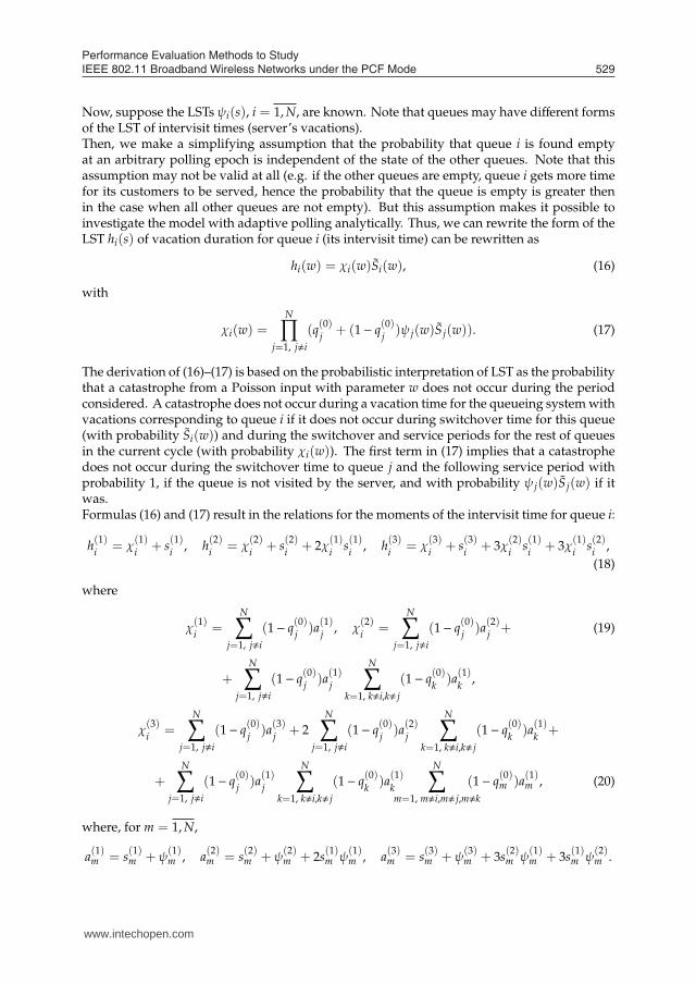
Here we give numerical examples to illustrate how the algorithm works for polling systemswith various numbers of queues and traffic intensity comparing to the simulation resultsobtained using the general-purpose simulation system GPSS World (Schriber, 1974). Theobject of modeling was represented by a regional broadband wireless network consisting ofseveral devices operating with one base station. The rates of packet arrivals to the devices andthe rate of processing them are different. The devices are polled cyclically. Packet servicingis gated, that is, only those packets are transmitted which were at the queue at the pollingmoment. The input flows are assumed to be of the Poisson nature, and the times of packetservicing and polling initialization are assumed to be exponentially distributed.We assume for simulation that the system is in the stationary mode when at duplication ofthe number of the packets passing through the system none of the comparison parameterschanges more than by 0.5%. In the experiments, more than three million of packets passedthrough the system.Average packet service time, switchover time, etc. in the numerical examples are taken fromthe real IEEE 802.11a broadband wireless network under PCF mode with realistic packet sizesand load levels. Thus, the obtained results correspond to such networks and mean waitingtimes satisfy the real systems requirements.Case N = 2. First, consider the symmetric system of two queues with the mean service times
b(1)1
= b(1)2
= 0.311, the mean switchover times s(1)1
= s(1)2
= 0.091 and the mean time of
server’s vacation ϕ(1) = 0.005. The mean waiting time calculated by the Algorithm (column"A"). Simulation results (column "S") and relative error of comparison (column "∆") are shownin Table 1. The first column describes the customers input intensities and the correspondingtraffic intensities. Two last lines of the Table present the results obtained for different mean
server’s vacation times ϕ(1) given that λ1 = λ2 = 0.5.
A S ∆, %λ1 = λ2 = 0.321, ρ = 0.2 0.289 0.268 7.8λ1 = λ2 = 0.5, ρ = 0.311 0.392 0.358 9.5λ1 = λ2 = 0.803, ρ = 0.5 0.659 0.601 9.7λ1 = λ2 = 1.28, ρ = 0.8 1.73 1.93 10.4
ϕ(1) = 0.05 0.392 0.358 9.5
ϕ(1) = 0.1 0.417 0.384 8.6
Table 1. System with two queues
Case N = 3. Now, consider the case of three queues with symmetric service b(1)i
= 0.044,
s(1)i
= 0.1, i = 1, 3, ϕ(1) = 0.1. The mean waiting times W(1)i
, i = 1, 3 obtained by using thealgorithm and simulation are presented in Table 2 for various customer input intensities. The
last two lines contain results for fully symmetric system (all λi, i = 1, 3 are the same).
www.intechopen.com
Performance Evaluation Methods to Study IEEE 802.11 Broadband Wireless Networks under the PCF Mode 531
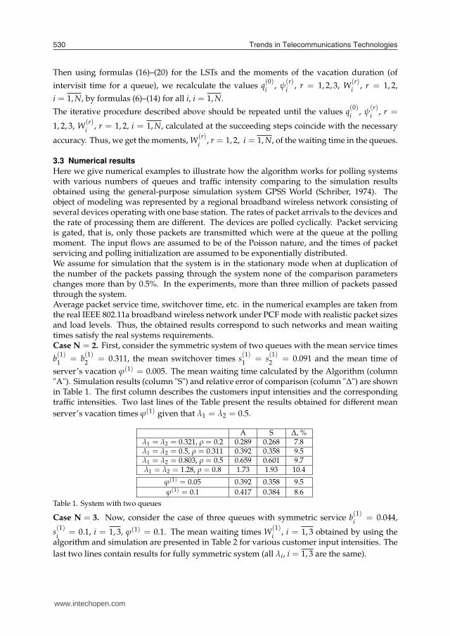
Case N = 5. And, finally, consider the case of five queues with λ1 = 1, λ2 = 2, λ3 = 0.5,
λ4 = 6, λ5 = 0.5, b(1)i
= 0.05, s(1)i
= 0.05, i = 1, 5, ϕ(1) = 0.05. We vary the input intensity bymultiplying all λi by αwhich takes values 0.285, 0.714, 1, and 1.143. Thus, the traffic intensity,ρ, varies from 0.2 to 0.8. The results are given in Table 3. The last four lines present results forthe fully symmetric system with λi = 2 multiplied by the same values of α.
A S ∆, % A S ∆, %λ1 = 2.5 0.342 0.365 6.3 λ1 = 4.375 0.658 0.698 5.7λ2 = 6 0.335 0.361 7.2 λ2 = 10.5 0.781 0.834 3.0λ3 = 0.5 0.410 0.440 6.8 λ3 = 0.875 0.778 0.805 3.4
Symmetric system
λi = 3, i = 1, 3 0.387 0.382 1.3 λi = 5.25, i = 1, 3 0.702 0.771 8.9
Table 2. System with three queues
A S ∆, % A S ∆, %
W(1)1
0.203 0.220 7.7 W(1)1
0.714 0.672 6.2
α = 0.285 W(1)2
0.199 0.215 7.4 α = 1 W(1)2
0.661 0.618 7.0
ρ = 0.2 W(1)3
0.205 0.222 7.7 ρ = 0.7 W(1)3
0.776 0.738 5.1
W(1)4
0.197 0.203 3.0 W(1)4
0.705 0.679 3.8
W(1)5
0.205 0.224 8.5 W(1)5
0.776 0.745 4.2
W(1)1
1.036 0.974 6.4 W(1)1
0.374 0.398 6.0
α = 0.714 W(1)2
0.353 0.370 4.6 α = 1.143 W(1)2
0.967 0.934 3.5
ρ = 0.5 W(1)3
0.393 0.419 6.2 ρ = 0.8 W(1)3
1.153 1.080 6.8
W(1)4
0.340 0.355 4.2 W(1)4
1.152 1.120 2.9
W(1)5
0.393 0.422 6.9 W(1)5
1.153 1.090 5.8
Symmetric system
ρ = 0.2 W(1)i
0.207 0.216 4.2 ρ = 0.7 W(1)i
0.759 0.686 10.6
ρ = 0.5 W(1)i
0.455 0.391 16.4 ρ = 0.8 W(1)i
1.003 1.040 3.6
Table 3. System with five queues
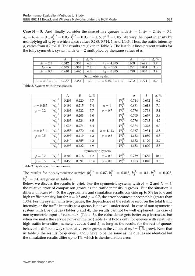
The results for non-symmetric service (b(1)1
= 0.07, b(1)2
= 0.015, b(1)3
= 0.1, b(1)4
= 0.025,
b(1)5
= 0.4) are given in Table 4.Below, we discuss the results in brief. For the symmetric systems with N = 2 and N = 3,the relative error of comparison grows as the traffic intensity ρ grows. But the situation isdifferent in case N = 5: the approximate and simulation results coincide up to 5% for low andhigh traffic intensity, but for ρ = 0.5 and ρ = 0.7, the error becomes unacceptable (grater than10%). For the system with five queues, the dependence of the relative error on the total trafficintensity, or the traffic intensity to a queue, is not well-understood. In case of non-symmetricsystem with five queues (Tables 3 and 4), the results can not be well explained. In case ofnon-symmetric input of customers (Table 3), the coincidence gets better as ρ increases, butwhen we make the service non-symmetric (Table 4), it holds only for queues with relativelyhigh traffic intensities, namely, queues 4 and 5, as long as the results for the rest of queues
behave the different way (the relative error grows as the values of ρi, i = 1, 3, grow). Note thatin Table 3, the results for queues 3 and 5 have to be the same as the queues are identical butthe simulation results differ up to 1%, which is the simulation error.
www.intechopen.com
Trends in Telecommunications Technologies532
A S ∆, % A S ∆, %
W(1)1
0.251 0.250 0.4 W(1)1
0.570 0.506 12.7
α = 0.4, W(1)2
0.248 0.244 1.6 α = 1, W(1)2
0.535 0.475 12.7
ρ = 0.2 W(1)3
0.251 0.254 1.2 ρ = 0.5 W(1)3
0.592 0.548 7.9
W(1)4
0.244 0.228 7.0 W(1)4
0.516 0.455 13.4
W(1)5
0.223 0.254 12.2 W(1)5
0.538 0.559 3.8
W(1)1
0.318 0.314 1.3 W(1)1
1.016 0.902 12.6
α = 0.6, W(1)2
0.311 0.302 3.0 α = 1.4, W(1)2
0.901 0.831 8.4
ρ = 0.3 W(1)3
0.322 0.325 0.9 ρ = 0.7 W(1)3
1.095 0.994 10.2
W(1)4
0.305 0.281 8.5 W(1)4
0.938 0.896 4.7
W(1)5
0.281 0.325 13.5 W(1)5
1.082 1.080 0.2
Table 4. System with five queues and non-symmetric service
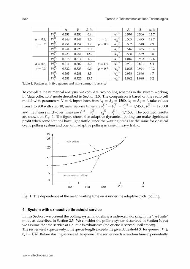
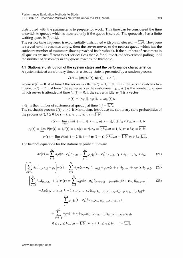
To complete the numerical analysis, we compare two polling schemes in the system workingin "data collection" mode described in Section 2.5. The comparison is based on the radio cellmodel with parameters N = 4, input intensities λ1 = λ2 = 1500, λ3 = λ4 = λ take values
from 1 to 200 with step 10, mean service times are b(1)1
= b(1)2
= b(1)4
= 1/4500, b(1)3
= 1/3000
and the mean switch-over times are s(1)1
= s(1)2
= s(1)3
= s(1)4
= 1/1500. The obtained resultsare shown on Fig. 1. The figure shows that adaptive dynamical polling can make significantprofit when some stations have light traffic, since the waiting times are the same for classicalcyclic polling system and one with adaptive polling in case of heavy traffic.
Fig. 1. The dependence of the mean waiting time on λ under the adaptive cyclic polling
4. System with exhaustive threshold service
In this Section, we present the polling system modelling a radio-cell working in the "last mile"mode as described in Section 2.5. We consider the polling system described in Section 3, butwe assume that the service at a queue is exhaustive (the queue is served until empty).The server visit a queue only if the queue length exceeds the given threshold (ki for queue i), ki ≥
0, i = 1, N. Before starting service at the queue i, the server needs a random time exponentially
www.intechopen.com
Performance Evaluation Methods to Study IEEE 802.11 Broadband Wireless Networks under the PCF Mode 533
distributed with the parameter si to prepare for work. This time can be considered the timeto switch to queue i which is incurred only if the queue is served. The queue also has a finitewaiting space hi (hi ≥ ki).
The service time in queue i is exponentially distributed with parameter µi, i = 1, N. The queueis served until it becomes empty, then the server moves to the nearest queue which has thesufficient number of customers (having reached its threshold). If the numbers of customers inall queues are insufficient to get service (less than ki for queue i), the server stops polling untilthe number of customers in any queue reaches the threshold.
4.1 Stationary distribution of the system states and the performance characteristics
A system state at an arbitrary time t in a steady-state is presented by a random process
ξ(t) = (m(t), i(t), n(t)), t ≥ 0,
where m(t) = 0, if at time t the server is idle, m(t) = 1, if at time t the server switches to aqueue, m(t) = 2, if at time t the server serves the customers, t ≥ 0; i(t) is the number of queuewhich server is attended at time t, i(t) = 0, if the server is idle; n(t) is a vector
n(t) = (n1(t), n2(t), . . . , nN(t)),
n j(t) is the number of customers at queue j at time t, j = 1, N.The stochastic process ξ(t), t ≥ 0, is Markovian. Introduce the stationary state probabilities of
the process ξ(t), t ≥ 0 for r = (r1, r2, . . . , rN), i = 1, N,
a(r) = limt→∞
P{m(t) = 0, i(t) = 0, n(t) = r}, 0 ≤ rm < km, m = 1, N,
pi(r) = limt→∞
P{m(t) = 1, i(t) = i, n(t) = r}, rm = 0, hm, m = 1, N, m � i, ri = ki, hi,
qi(r) = limt→∞
P{m(t) = 2, i(t) = i, n(t) = r}, 0, hm, m = 1, N, m � i, ri1, hi.
The balance equations for the stationary probabilities are
λa(r) =N∑
j=1
λ ja(r− e j)I{r j>0} +N∑
j=1
µ jq j(r + e j)I{r j=0}, r1 < k1, . . . , rN < kN , (21)
N∑
m=1
λmI{rm<hm} + µi
qi(r) =N∑
j=1
λ jqi(r− e j)I{r j>δi j} + µiqi(r + ei)I{ri<hi} + sipi(r)I{ri≥ki}, (22)
N∑
m=1
λmI{rm<hm} + si
pi(r) =N∑
j=1
λ jpi(r− e j)I{r j>kiδi j} + µi−1qi−1(r + ei−1)I{ri−1=0}+ (23)
+λia(r1, . . . , ri−1, ki − 1, ri+1, . . . , rN)I{r1<k1,...,ri−1<ki−1,ri=ki,ri+1<ki+1,...,rN<kN}+
+i−2∑
j=1
µ jq j(r + e j)I{r j=0,r j+1<k j+1,...,ri−1<ki−1}+
+N∑
j=i+1
µ jq j(r + e j)I{r j=0,r j+1<k j+1,...,rN<kN ,r1<k1,...,ri−1<ki−1},
0 ≤ rm ≤ hm, m = 1, N, m � i, ki ≤ ri ≤ hi, i = 1, N.
www.intechopen.com
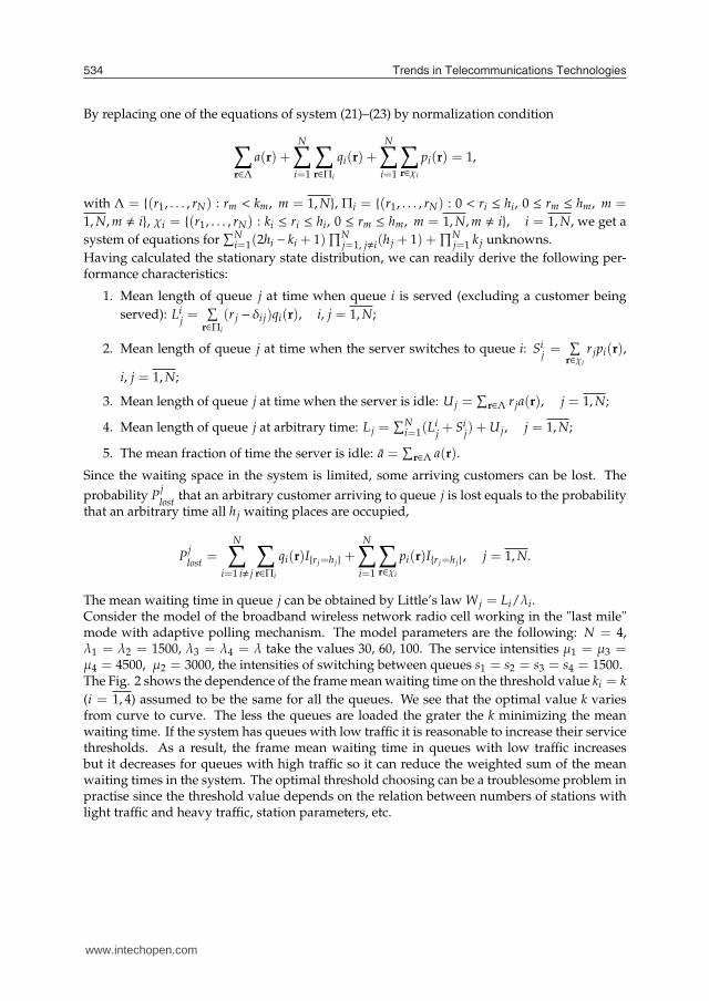
Trends in Telecommunications Technologies534
By replacing one of the equations of system (21)–(23) by normalization condition
∑
r∈Λ
a(r)+N∑
i=1
∑
r∈Πi
qi(r) +N∑
i=1
∑
r∈χi
pi(r) = 1,
with Λ = {(r1, . . . , rN) : rm < km, m = 1, N}, Πi = {(r1, . . . , rN) : 0 < ri ≤ hi, 0 ≤ rm ≤ hm, m =
1, N, m � i}, χi = {(r1, . . . , rN) : ki ≤ ri ≤ hi, 0 ≤ rm ≤ hm, m = 1, N, m � i}, i = 1, N, we get a
system of equations for∑N
i=1(2hi − ki + 1)∏N
j=1, j�i(h j + 1) +∏N
j=1 k j unknowns.
Having calculated the stationary state distribution, we can readily derive the following per-formance characteristics:
1. Mean length of queue j at time when queue i is served (excluding a customer being
served): Lij=∑
r∈Πi
(r j − δi j)qi(r), i, j = 1, N;
2. Mean length of queue j at time when the server switches to queue i: Sij=∑
r∈χi
r jpi(r),
i, j = 1, N;
3. Mean length of queue j at time when the server is idle: U j =∑
r∈Λ r ja(r), j = 1, N;
4. Mean length of queue j at arbitrary time: L j =∑N
i=1(Lij+ Si
j) + U j, j = 1, N;
5. The mean fraction of time the server is idle: a =∑
r∈Λ a(r).
Since the waiting space in the system is limited, some arriving customers can be lost. The
probability Pj
lostthat an arbitrary customer arriving to queue j is lost equals to the probability
that an arbitrary time all h j waiting places are occupied,
Pj
lost=
N∑
i=1 i� j
∑
r∈Πi
qi(r)I{r j=h j} +N∑
i=1
∑
r∈χi
pi(r)I{r j=h j}, j = 1, N.
The mean waiting time in queue j can be obtained by Little’s law W j = Li/λi.Consider the model of the broadband wireless network radio cell working in the "last mile"mode with adaptive polling mechanism. The model parameters are the following: N = 4,λ1 = λ2 = 1500, λ3 = λ4 = λ take the values 30, 60, 100. The service intensities µ1 = µ3 =µ4 = 4500, µ2 = 3000, the intensities of switching between queues s1 = s2 = s3 = s4 = 1500.The Fig. 2 shows the dependence of the frame mean waiting time on the threshold value ki = k
(i = 1, 4) assumed to be the same for all the queues. We see that the optimal value k variesfrom curve to curve. The less the queues are loaded the grater the k minimizing the meanwaiting time. If the system has queues with low traffic it is reasonable to increase their servicethresholds. As a result, the frame mean waiting time in queues with low traffic increasesbut it decreases for queues with high traffic so it can reduce the weighted sum of the meanwaiting times in the system. The optimal threshold choosing can be a troublesome problem inpractise since the threshold value depends on the relation between numbers of stations withlight traffic and heavy traffic, station parameters, etc.
www.intechopen.com
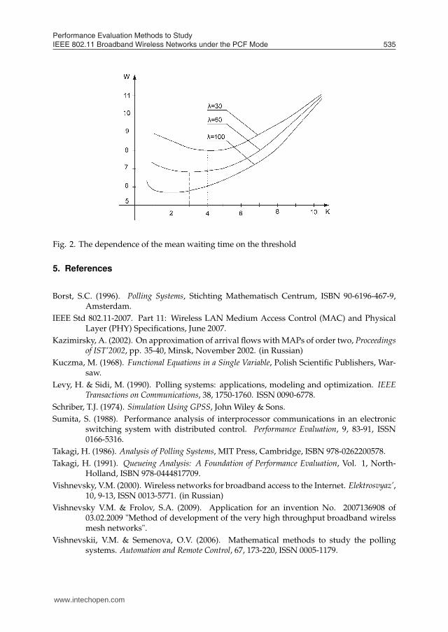
Performance Evaluation Methods to Study IEEE 802.11 Broadband Wireless Networks under the PCF Mode 535
Fig. 2. The dependence of the mean waiting time on the threshold
5. References
Borst, S.C. (1996). Polling Systems, Stichting Mathematisch Centrum, ISBN 90-6196-467-9,Amsterdam.
IEEE Std 802.11-2007. Part 11: Wireless LAN Medium Access Control (MAC) and PhysicalLayer (PHY) Specifications, June 2007.
Kazimirsky, A. (2002). On approximation of arrival flows with MAPs of order two, Proceedingsof IST’2002, pp. 35-40, Minsk, November 2002. (in Russian)
Kuczma, M. (1968). Functional Equations in a Single Variable, Polish Scientific Publishers, War-saw.
Levy, H. & Sidi, M. (1990). Polling systems: applications, modeling and optimization. IEEETransactions on Communications, 38, 1750-1760. ISSN 0090-6778.
Schriber, T.J. (1974). Simulation Using GPSS, John Wiley & Sons.
Sumita, S. (1988). Performance analysis of interprocessor communications in an electronicswitching system with distributed control. Performance Evaluation, 9, 83-91, ISSN0166-5316.
Takagi, H. (1986). Analysis of Polling Systems, MIT Press, Cambridge, ISBN 978-0262200578.
Takagi, H. (1991). Queueing Analysis: A Foundation of Performance Evaluation, Vol. 1, North-Holland, ISBN 978-0444817709.
Vishnevsky, V.M. (2000). Wireless networks for broadband access to the Internet. Elektrosvyaz’,10, 9-13, ISSN 0013-5771. (in Russian)
Vishnevsky V.M. & Frolov, S.A. (2009). Application for an invention No. 2007136908 of03.02.2009 "Method of development of the very high throughput broadband wirelssmesh networks".
Vishnevskii, V.M. & Semenova, O.V. (2006). Mathematical methods to study the pollingsystems. Automation and Remote Control, 67, 173-220, ISSN 0005-1179.
www.intechopen.com

Trends in Telecommunications Technologies536
Vishnevskii, V.M. & Semenova, O.V. (2007). Polling Systems: Theory and Applications for Broad-band Wireless Networks, Moscow, Technosphera, ISBN 978-5-94836-166-6. (in Russian)
Vishnevsky, V.M.; Portnoy, S.L. & Shakhnovich, I.V. (2009). Encyclopaedia WiMAX. Way to 4G,Moscow, Technosphera. (in Russian)
www.intechopen.com
Trends in Telecommunications TechnologiesEdited by Christos J Bouras
ISBN 978-953-307-072-8Hard cover, 768 pagesPublisher InTechPublished online 01, March, 2010Published in print edition March, 2010
InTech EuropeUniversity Campus STeP Ri Slavka Krautzeka 83/A 51000 Rijeka, Croatia Phone: +385 (51) 770 447 Fax: +385 (51) 686 166www.intechopen.com
InTech ChinaUnit 405, Office Block, Hotel Equatorial Shanghai No.65, Yan An Road (West), Shanghai, 200040, China
Phone: +86-21-62489820 Fax: +86-21-62489821
The main focus of the book is the advances in telecommunications modeling, policy, and technology. Inparticular, several chapters of the book deal with low-level network layers and present issues in opticalcommunication technology and optical networks, including the deployment of optical hardware devices and thedesign of optical network architecture. Wireless networking is also covered, with a focus on WiFi and WiMAXtechnologies. The book also contains chapters that deal with transport issues, and namely protocols andpolicies for efficient and guaranteed transmission characteristics while transferring demanding dataapplications such as video. Finally, the book includes chapters that focus on the delivery of applicationsthrough common telecommunication channels such as the earth atmosphere. This book is useful forresearchers working in the telecommunications field, in order to read a compact gathering of some of thelatest efforts in related areas. It is also useful for educators that wish to get an up-to-date glimpse oftelecommunications research and present it in an easily understandable and concise way. It is finally suitablefor the engineers and other interested people that would benefit from an overview of ideas, experiments,algorithms and techniques that are presented throughout the book.
How to referenceIn order to correctly reference this scholarly work, feel free to copy and paste the following:
Vladimir Vishnevsky and Olga Semenova (2010). Performance Evaluation Methods to Study IEEE 802.11Broadband Wireless Networks under the PCF Mode, Trends in Telecommunications Technologies, Christos JBouras (Ed.), ISBN: 978-953-307-072-8, InTech, Available from: http://www.intechopen.com/books/trends-in-telecommunications-technologies/performance-evaluation-methods-to-study-ieee-802-11-broadband-wireless-networks-under-the-pcf-mode

© 2010 The Author(s). Licensee IntechOpen. This chapter is distributedunder the terms of the Creative Commons Attribution-NonCommercial-ShareAlike-3.0 License, which permits use, distribution and reproduction fornon-commercial purposes, provided the original is properly cited andderivative works building on this content are distributed under the samelicense.