PERFORMANCE EVALUATION OF peA TESTS IN … Evaluation of... · ERROR IDENTIFICATION 123 In both PCNT and PCMT, the measurements in gross errors can further he identified by looking

Chern. Eng. Comm., 2000, Vol. 183, PI'. 119-139Reprints available directly from the publisherPhotocopying permitted by license only

et> 2000 OPA (Overseas Publishers Association) N.V.Published by license under

the Gordon and Breach SciencePublishers imprint.

Printed in Malaysia.

PERFORMANCE EVALUATIONOF peA TESTS IN SERIAL ELIMINATION

STRATEGIES FOR GROSSERROR IDENTIFICATION

MIGUEL BAGAJEWICZa,. , QIYOU JIANGa

and MABEL SANCHEZb

"School of Chemical Engineering and Materials Science, University of Oklahoma.Norman, OK. USA: bPlanta Piloto de lngenieria Quimica (UNS - CONICET) ,

Camino La Carrindanga. Km 7, (8000) Bahia Blanca-Argentina

( Received 28 December 1999: In final form 10 April 2000)

In this paper, the performance of the Principal Component Measurement Test (PCMT) isevaluated when used for the identification of multiple biases. A serial elimination strategy isimplemented where a statistical test based on principal component analysis is used to identifythe measurement to eliminate. A simulation procedure involving random measurement errorsand fixed gross error sizes is applied to evaluate its performance. This performance is comparedwith the one obtained using serial elimination using the conventional Measurement Test (MT),as it is performed in some commercial simulators. The analysis indicates that principal component tests alone, without the aid of other collective tests, do not significantly enhance theability in identification features of this strategy. performing worse in some cases. A few cases ofsevere failure of this strategy are shown and a suggestion to test other strategies is offered.

Keywords: Data reconciliation; Gross errors; Principal component analysis

INTRODUCTION

Data reconciliation techniques are performed to estimate process variablesin such a way that balance constraints are satisfied, but to obtain accurateestimates, some action should be taken to eliminate the influence of grosserrors. Hypothesis testing has been extensively used for detection and

·Corresponding author. Tel.: 4053255458, Fax: 4053255813, e-mail: [email protected]

119

Downloaded By: [EBSCOHost EJS Content Distribution - Superceded by 916427733] At: 17:45 4 September 2010

120 M. BAGAJEWICZ et 01.

identification purposes. A good survey of this issue can be found in Mah(1990) and Madron (1992).

For the purpose of identification of gross errors, Mah (1982) proposedthe measurement test. This test has been used in gross error hypothesis testing in almost all practical applications. Narasimhan and Mah (1987) introduced the GLR test, which can also provide an estimate of the gross error.Crowe (1988) proved that these two are equivalent and have maximumpower for the case of one gross error. Recently Principal Component Tests(PCT) have been proposed by Tong and Crowe (1995, 1996) as analternative for multiple bias and leak identification. Industrial applicationsofPCMT were reported by Tong and Bluck (1998), who indicated that testsbased on PCA are more sensitive to subtle gross errors than others, andhave larger power to correctly identify the variables in error than theconventional Nodal, Measurement and Global Tests. With the exceptionof the aforementioned scattered examples of improved efficiency for onegross error, there is no published work assessing the effectiveness of themethod for multiple gross errors.

For the case of multiple gross errors, serial elimination was originallyproposed by Ripps (1965). The method proposes to eliminate the measurement that renders the largest reduction in a test statistics until notest fails. Several authors proposed different variants of this procedure(Nogita, 1972; Romagnoli and Stephanopoulos, 1981; Crowe et al., 1983;Rosenberg et al., 1987). Of all these strategies, the one that has beenimplemented in commercial software more often is the one where thelargest measurement test (MT) is used to determine the measurement toeliminate.

The increasing application of PCA in process monitoring and faultdiagnosis, and the lack of performance evaluation studies like those proposed by Iordache et al. (1985), Serth and Heenan (1986), motivates thepresent work. It involves a comparison of the identification performance ofPCMT and MT for existing industrial plants, where multiple gross errorsare present. The strategy presented does not include recommendationsperformed by Tong and Crowe (1995) to complement the usage of thePCMT with information from collective tests. Incorporating such tests inour scheme would not constitute a fair comparison, neither for the usageof PC, nor for the usage of the measurement test.

The paper is organized as follows. First, the PCT is reviewed followed bya short description of the serial elimination strategy and the new strategytested. Finally, performance evaluation results and a comprehensive discussion are provided.


ERROR IDENTIFICAnON

PRINCIPAL COMPONENT TESTS

121

In this section, a review of principal component tests proposed by Tong andCrowe (1995) is presented. The Principal Component Nodal Test (PCNT) andthe Principal Component Measurement Test (PCMT) are briefly described.

Given a linear steady-state process, the residuals of the constraints aredefined as

r=Ay (I)

where y is the vector of measurements and A the balance matrix. Forsimplicity, in this formulation it is assumed that all variables are measured.This is not a limitation since the unmeasured variables can be removedusing, for example, the Reduced Balance Scheme (Vaclavek, 1969), MatrixProjection (Crowe, 1983), QR decomposition (Schwartz, 1989); (Sanchezand Romagnoli, 1996) or Matrix co-optation (Madron, 1992).

Assuming that the measurement errors follow a certain distribution withcovariance '11 then r will follow the same distribution with expectation andcovariance given by

E{r} = r' = 0 <I> = cov{r} = AWAT

The eigenvalue decomposition of matrix ~ is formulated as

Ar = U;ipUr

where,

U,: matrix of orthonormalized eigenvectors of <I>(UrU; = I)Ar: diagonal matrix of the eigenvalues of <1>.

Accordingly, the following linear combinations of r are proposed

p' = W;(r - r*) = W;r

where,

W, = UrA; I/2

(2)

(3)

(4)

(5)

and p' consists of the principal components. Also, r ~ P(O, ip) => p' I"V P(O, I),for any distribution P. That is, a set of correlated variables r is transformedinto a new set of uncorrelated variables pro If the measurement errorsare normally distributed then the principal components will be normallydistributed too. That is: y ~ N(x, '11) ~ p'~ N(O, I). Consequently, instead of


122 M. BAGAJEWICZet al.

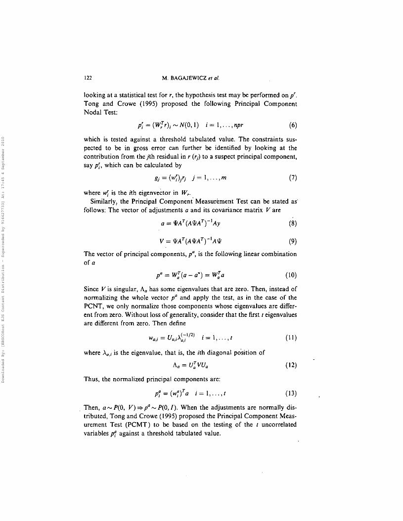
looking at a statistical test for T, the hypothesis test may be performed on proTong and Crowe (1995) proposed the following Principal ComponentNodal Test:

p~ = (W;'r)i rv N(0I 1) i = 1, ... 1 npr (6)

which is tested against a threshold tabulated value. The constraints suspected to be in gross error can further be identified by looking at thecontribution from the jth residual in r (rj) to a suspect principal component,say p~, which can be calculated by

(7)

where »1 is the ith eigenvector in W,.Similarly, the Principal Component' Measurement Test can be stated as'

follows: The vector of adjustments a and its covariance matrix V are

(8)

(9)

The vector of principal components, p", is the following linear combinationof a

pO = WJ(a - a*) = W~a (10)

Since V is singular, Aa has some eigenvalues that are zero. Then, instead ofnormalizing the whole vector pO and apply the test, as in the case of thepeNT, we only normalize those components whose eigenvalues are different from zero. Without loss of generality, consider that the first t eigenvaluesare different from zero. Then define

(11)

where Aa ,; is the eigenvalue, that is, the ith diagonal position of

s, = U~VUo (12)

Thus, the normalized principal components are:

a (Q)T . 1Pi = Wi a I = I"" t (13)

. Then, a rv P(O, V) ~ pO rv P(O, I). When the adjustments are normally distributed, Tong and Crowe (1995) proposed the Principal Component Measurement Test (PCMT) to be based on the testing of the t uncorrelatedvariables pf against a threshold tabulated value.


ERROR IDENTIFICATION 123

In both PCNT and PCMT, the measurements in gross errors can furtherhe identified by looking at the contribution from the jth residual/adjustmentto a suspect principal component, say, rt. This contribution is calculatedas follows:

(14)

To assess the number of major contributors k, for a suspect principalcomponent pf, a vector g' is defined that contains the elements gj in descending order of their absolute values. Then k l is set so that

(15)

where ~ may be fixed, for example at 0.1.

REVIEW OF SERIAL ELIMINATION STRATEGY

Serial elimination was originally proposed by Ripps (1965). The methodproposed to eliminate the measurement that renders the largest reductionin the Chi-squared statistics and then repeat the procedure eliminatingmeasurements one at a time until the maximum number of measurementsallowed to be deleted is reached or the statistics falls below the thresholdvalue. Nogita (1972) later modified this approach by proposing to eliminatethe measurement that reduces the objective function the most and stoppingwhen the objective function increases or the maximum of deletions has beenreached. Romagnoli and Stephanopoulos (1981) proposed a method to reevaJuate the objective function without having to solve the reconciliationagain and obtain an estimate of the gross errors. Additionally, Crowe et al.

(1983) proposed a strategy where the global test is used in conjunction withother test statistics. Rosenberg et al. (1987) presented an extension of themethod where instead of only one measurement being deleted at a time, setsof measurements of different size are deleted. We now present Rosenberget a/.'s version of the aJgorithm followed by the version of Serial Eliminationbased on the measurement test that is used in many commercial packages.

Serial Elimination Strategy Based on the Global Test (SEG)

The basis of the method is that measurements are deleted sequentially ingroups of size d, t = 1,2 ... ,dmax ' After each deletion, the process constraints


124 M. BAGAJEWICZ et al.

are projected (matrix A is recalculated) and the global test is againapplied. This procedure continues until among all sets of measurementsthat are deleted one can find one for which the global test indicates nogross error, or until dmax is reached. In this last case, the set that produces the largest reduction in test statistics is declared as the set of grosserrors.

Let the following be defined:

S: set of all measured stream flow ratesSd: temporary set which contains the measurements being deleted in a

particular step,Sc: current set of measurements suspected of containing gross

errors.d max: maximum number of measurements that can be deleted from the

original network so that the degree of freedom of the constraints isequal to one (rank A = 1). This is equivalent to leave the system withone degree of redundancy.

Fmin: area under the Chi-square distribution that represents the desireddegree of confidence.

The gross error identification steps are:

A. Determine d max- Set d =0 and S; =o.B. Determine the degrees of freedom, ZI, for the network contairung the

measurement set S, and calculate the global test statistic, T = ,Ttf> -1r. IfT < X~ta' declare no gross errors and stop. Otherwise, go to Step C.

C. Set d= d+ l. If d » d max declare all measurements in S suspect and stop.Otherwise, set Fm in = I-a. For each possible combination Sd of dmeasurements, do the following:

(a) Delete the set Sd from the network.

(b) Obtain the new constraint matrix A to reflect the reduced set ofmeasurements, S - Sd' If one or more columns of the new matrix A arezero, discard this set Sd and choose the next set of d measurements.

(c) Determine the degrees of freedom v for the projected constraints, i.e., therank of A. Calculate the global test statistic T for the projectedconstraints.

(d) If F{X~} < Fmin, replace s. by e,and reset Fmin = F{X~}. If all sets of dmeasurements have been tried, go to D. Otherwise, choose the next set ofd measurements in Step (a).

D. If Fmi n < I - a, declare all measurements in S; in suspect and stop.Otherwise, go to Step C.



Serial Elimination Strategy Based on the Measurement Test (SEM)

The serial elimination strategy based on measurement test (SEM) is obtainedbased on the modification of SEG. The gross error identification steps are:

A. Determine d m ax • Set d=O and Sc=O.

B. Run the data reconciliation and calculate the measurement test (MT)statistics. If no MT flags, declare no gross errors and stop. Otherwise, go toStep C.

C. If the number of elements in S; > d max declare all measurements in Scsuspect and stop. Otherwise, put the stream with the largest MT into S; anddo the following:

(a) Delete the set S, from the network.

(b) Obtain the new constraint matrix A to reflect the reduced set ofmeasuremen ts, S - SC'

(c) Do the data reconciliation and calculate MT for the new redundantsystem.

D. If no MT flags, declare all measurements in Sc in suspect and stop.Otherwise, go to Step C.

MODIFICATION OF SEM TO USE PCMT

In order to compare the performance of MT and PCMT in the serialelimination strategy, the serial elimination strategy based on PCMT, whichis called PCMT - SEM in this paper, is proposed.

The procedure is:

A. Determine d max. Set d=O and Sc=O.

B. Run the data reconciliation and calculate the PCMT statistics. If no PCMTflags, declare no gross errors and stop. Otherwise, go to Step C.

C. If the number of elements in S; > d max, declare all measurements in Sc

suspect and stop. Otherwise put the stream with the largest contribution tothe largest PCMT into S; and do the following:

(a) Delete the set S, from the network.

(b) Obtain the new constraint matrix B to reflect the reduced set ofmeasurements, S - SC'

(c) Do the data reconciliation and calculate PCMT for the new redundantsystem.

D. If no PCMT flags, declare all measurements in Sc in suspect and stop.Otherwise, go to Step C.


126 M. BAGAJEWICZ et 01.

SIMULATION PROCEDUREAND UNCERTAINTY REMOVAL

A simulation procedure was applied to evaluate the performance of theaforementioned strategies. The method proposed by Iordache et al. (1985)was followed. Each result is based on 10000 simulation trials where therandom errors are changed and the magnitudes of gross errors are fixed.

Three performance measures are used: overall power (OP), averagenumber of Type I errors (AVTI) and expected fraction of perfect identification (OPF). They are defined as follows:

ONo. of gross errors correctly identifiedp=---------------

No. of gross errors simulated

A VTI = No. of gross errors incorrectly identifiedNo. of simulation trials

O F= No. of trials with perfect identification

p f' l' . INo. 0 simu anon tna s

(16)

( 17)

(18)

The first two measures are proposed by Mah and Narasimhan (1987) andthe last one by Rollins and Davis (1992).

A set of gross errors may have its equivalent sets, as describedby Bagajewicz and Jiang (1998). Thus, to assess these uncertainties, a newmeasure, the overall performance of equivalent identification (OPFE) wasintroduced recently (Sanchez et al., 1999).

OPFE = No. of triaJs with successful identification (19)No. of simulation trials

Determination of 0 PFE

The uncertainty in gross error detection was discussed in a recent paper(Bagajewicz and Jiang, 1998). Two sets of gross errors are considered equivalent when they have the same effect in data reconciliation. Equivalentsets usually have the same gross error cardinality. However, in some caseswhen a set of gross errors has special sizes (usually equal to each other) itcan be represented by another set of gross errors with different cardinality.These cases are caJJed Degenera teo

When a set of gross errors is obtained, one can identify if it is a successfulidentification by simply applying the conversion equation between equivalent


ERROR IDENTIFICATION

sets, which has been proposed by Jiang and Bagajewicz (1999):

127

(20)

where A is the incidence matrix, g1, it vectors of biases and leaks for the setof gross errors identified, 82, i2 vectors of biases and leaks for the set ofgross errors introduced, L t , K., L 2, K2 matrices reflecting the positions ofbiases and leaks in the system.

Pre-multiplying both [ALI Kd and [AL2 K2] by a certain particularmatrix, one can transform [AL2 K 2] into a canonical form, and obtain thenew gross error sizes 82 and 1'2'

In addition, sometimes many sets of gross errors can represent degeneracyif certain tolerance is allowed. These situations are called Quasi-Degeneracy(Jiang and Bagajewicz, 1999). For example, consider the flowsheet ofFigure I. In particular consider one existing gross error in S2 of size82 = -1. Consider now that a particular gross error identification methodfinds gross errors in S4 and Ss of sizes 84 = + 1, 85 == + 1. These variablesare part of the equivalent set (82, 84, S5), which has gross error cardinality 2.To determine whether the identification is successful one should be ableto convert from the set of gross errors found to the originally introduced.In this case, this is possible because, by virtue of degeneracy, the two identified gross errors are equivalent to 82 = - 1.

Quasi-degeneracy takes place when for example the gross errors foundare of sizes 84 = + 0.98, 8s= + 1.01. Strictly, this set does not represent adegenerate case. Rather, the conversion to an equivalent set containing 82,

as for example (S2 85) , gives values 82 = - 0.98, 85 = - 0.01. Therefore, if 85

is ignored because its size is too small compared to a tolerance, the grosserror introduced are retrieved and it can be claimed that the identificationwas successful.

FIGURE 1


128 M. BAGAJEWlCZ et al.

In Eq. (20), both sides are vectors. Strictly, when quasi degeneracy is notallowed, both sides have to be equal to declare a successful identification.When Quasi-degeneracy is allowed, both sides are compared within certainthreshold tolerance CD.

Quasi Equivalency

Consider the following example. Assume that in Figure 1, a gross error isintroduced in stream SI of size 61= + 1. Assume also that the gross erroridentification finds two gross errors in SI and S2, with sizes 61 = +0.98,62 = +0.05. This is a type I error, but accompanied with a small size estimate.In principle, although the result is based on the usage of statistical tests, oneis tempted to disregard 62 and declare the identification successful. Oneimportant observation in this case is that SI and S2 are not a basic set of anysubset of the graph. In other words, no degeneracy or equivalency can apply.

Thus, generalizing Quasi-equivalency occurs when only a subset of theidentified gross errors is equivalent to the introduced gross errors, and inaddition, the nonequivalent gross errors are of small size. Quasi-equivalencyis also detected using Eq. (20) and a threshold tolerance eE.

OPFE is calculated in this paper by allowing both Quasi-Degeneracyand Quasi-equivalency.

RESULTS

The process flowsheet in Figure 2 is used with comparative purposes. Itconsists of a recycle system with five units and nine streams. The true flowrate values are x =[10. 20. 30. 20. 10. 10. 10. 4. 6.]. The flow rate standarddeviations were taken as 2% of the true flow rates.

Measurement values for each simulation trial were taken as the average often random generated values. In order to compare results on the same basis,

FIGURE 2 An example.



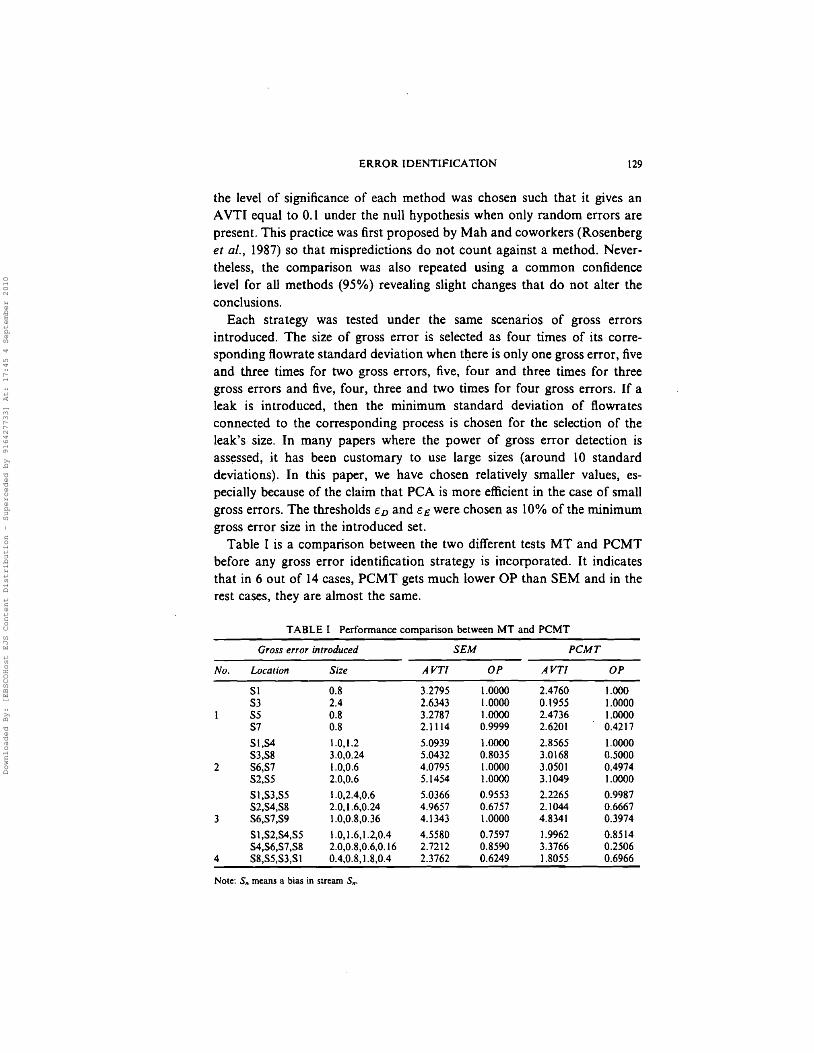
the level of significance of each method was chosen such that it gives anAVTI equal to 0.1 under the null hypothesis when only random errors arepresent. This practice was first proposed by Mah and coworkers (Rosenberget a/., 1987) so that mispredictions do not count against a method. Nevertheless, the comparison was also repeated using a common confidencelevel for all methods (950/0) revealing slight changes that do not alter theconclusions.

Each strategy was tested under the same scenarios of gross errorsintroduced. The size of gross error is selected as four times of its corresponding flowrate standard deviation when there is only one gross error, fiveand three times for two gross errors, five, four and three times for threegross errors and five, four, three and two times for four gross errors. If aleak is introduced, then the minimum standard deviation of ftowratesconnected to the corresponding process is chosen for the selection of theleak's size. In many papers where the power of gross error detection isassessed, it has been customary to use large sizes (around 10 standarddeviations). In this paper, we have chosen relatively smaller values, especially because of the claim that PCA is more efficient in the case of smallgross errors. The thresholds cn and C£ were chosen as 10% of the minimumgross error size in the introduced set.

Table I is a comparison between the two different tests MT and PCMTbefore any gross error identification strategy is incorporated. It indicatesthat in 6 out of 14 cases, PCMT gets much lower OP than SEM and in therest cases, they are almost the same.

TABLE I Performance comparison between MT and PCMT

Gross error introduced SEM PCMT

No. Location Size AVTl OP AVTI OP

51 0.8 3.2795 1.0000 2.4760 1.00053 2.4 2.6343 1.0000 0.1955 1.000055 0.8 3.2787 1.0000 2.4736 1.000057 0.8 2.1114 0.9999 2.6201 0.4217

51,54 1.0,1.2 5.0939 1.0000 2.8565 1.000053,58 3.0,0.24 5.0432 0.8035 3.0168 0.5000

2 56,S7 1.0,0.6 4.0795 1.0000 3.0501 0.497452,55 2.0,0.6 5.1454 1.0000 3.1049 1.0000

51,53,55 1.0,2.4,0.6 5.0366 0.9553 2.2265 0.998752,54,58 2.0,1.6,0.24 4.9657 0.6757 2.1044 0.6667

3 56,57,59 1.0,0.8,0.36 4.1343 1.0000 4.8341 0.3974

Sl,52,S4,S5 1.0,1.6,1.2,0.4 4.5580 0.7597 1.9962 0.851454,56,57,58 2.0,0.8,0.6,0.16 2.7212 0.8590 3.3766 0.2506

4 58,55,53,51 0.4,0.8,1.8,0.4 2.3762 0.6249 1.8055 0.6966

Note: SIt means a bias in stream SrI'



Table II shows the comparison between SEM and PCMT -SEM. Whenthere is one gross error, both of them reached high and similar performance.For more than one gross errors, the OPF for the two methods drops to lowvalues, reaching zero for the most cases of four gross errors. However, theOPFE for PCMT- SEM is slightly higher in most cases. The AVTI ofall theseruns is substantially large for the case of many gross errors. This indicatesan average large Type I error. However, these are based on consideringthe criterion of perfect identification. Within these "failures" there aregross errors that are equivalent to the introduced. A different version ofAVTI in which all equivalent and degenerate identifications are considered as successful would show lower values consistent with the largeOPFE scores.

The overall conclusion that one can make after examining all theseperformance measures is that PCA is of help in some situations and it doesnot make a difference in others. Moreover, it performs poorly in some cases.

The second example is a Large Plant example. It consists of 93 streams(3 of them are unmeasured: S46, 849 and 850), 11 processes, 14 tanks and9 nodes. Real data was used to perform data reconciliation and then thereconciled data were used as true values in our experiments. This adjusteddata are shown in the Appendix. The measurement values for eachsimulation trial were taken as the average of 10 random generated values.Considering the time expense for this large system, in this experimenteach result is based on 1000 (rather than 10000) simulation trials wherethe random errors are changed and the magnitudes of gross errors arefixed.

Table III indicates that in 5 out of the total 7 cases PCMT - SEM wassuccessful and got a slightly higher performance than SEM. However, thereare two cases that PCMT -SEM completely failed, while SEM was stillsuccessful.

The failure 'can be explained inn light of the PCA strategy. Theassumption that the variable with larger contribution to the larger principal component has larger probability of having a gross error is notalways true. We now show the details of case 4, which illustrate thisassertion.

(1) First iteration

(a) Number of principal components: 31(b) Suspect principal components and their corresponding major

contributions (both principal components and contributions aresorted from large to small absolute size):


Principal Component238272520


Major ContributionsS15, 814874, 524, 823, 888513, S14, S12, SIS814, SIS, 826514, SIS, S36, S29

131

(c) List of candidates: 515, 514, 874, 824, 823, 588, 813, 812, 826, S36,S29

(d) Stream to be deleted: S15.

(2) Second iteration


contributions:


Major ContributionsS14S74, 823, S24, S88S13, 514, 512814814, 829, S36, S71

(c) List of candidates: S14, 574, S23, S24, S88, 513, S12, 529, 836, S71(d) Stream to be deleted: S14.

(3) Third iteration


contributions:


Major Contributions574, S23, S24, S88

(c) List of candidates: S74, S23, 824, 888(d) Stream to be deleted: 874.

In this step, the size of principal component 8 is - 7.077 and thecontributions from S74 and 523 are -2.793 and -1.377 respectively. Thewrong candidate S74 is selected.



(4) Fourth iteration


contributions:


Major Contributions824,823

(c) List of candidates: 824, S23(d) Stream to be deleted: S24.

(5) Fifth iteration


contributions:


Major ContributionsS37, S~9, S17, S34, S79, S30, S42

(c) List of candidates: S37, S29, 817, S34, S79, 830, 842(d) Stream to be deleted: 837.

(6) Sixth iteration

(a) Number of principal components: 26(b) Suspect principal components: None.

(7) Identified gross errors: SIS, S14, 874, S24, 837.

Remark 1 The failure of case 4 a/so indicates a case of failure of identi-fication of one single component. Indeed, if the measurements in streams814 and Sl5 are eliminated and the gross error in 823 is left, then thesystem has only one gross error. The principal component test will have S23in it suspect candidate, but a serial elimination strategy would fail to identifyit as the variable in gross error.

Remark 2 In the absence of other tests, not picking the largest contributionto the largest principal component has a combinatorial method as analternative. If all the contributions need to be considered, a procedure hasto be implemented to sort out this list of candidates and identify one.


TABLE II Performance comparison between SEM and PCMT-SEM

Gross error introduced SEM PCMT-SEM

No. Location Size AVTI OP OPF OPFE AVTI OP OPF OPFE

SI 0.8 0.0910 1.0000 0.9107 0.9107 0.0881 1.0000 0.9167 0.9167S3 2.4 0.0793 1.0000 0.9225 0.9225 0.0878 1.0000 0.9187 0.9187S5 0.8 0.0939 1.0000 0.9077 0.9077 0.0917 1.0000 0.9122 0.912287 0.8 0.0984 0.9786 0.9057 0.9065 2.0267 0.0000 0.0000 0.8594L3 0.8 2.0658 0.0000 - 0.9157 3.0131 0.0000 - 0.8712

81,S4 1.0,1.2 0.0725 0.9988 0.9300 0.9313 0.0745 1.0000 0.9296 0.9296S3,S8 3.0,0.24 0.1045 0.9526 0.8500 0.8500 2.2411 0.5000 0.0000 . 0.1190

2 S6$7 1.0,0.6 0.1580 0.9444 0.8437 0.8461 3.0680 0.0000 0.0000 0.8929S2,S5 2.0.0.6 0.0788 1.0000 0.9219 0.9219 0.0811 1.0000 0.9225 0.9225S4,L2 2.0,0.6 2.0057 0.5000 - 0.8551 2.0316 0.5000 0.9133

51,83,55 1.0,2.4,0.6 0.9061 0.9638 0.2871 0.3704 0.0601 1.0000 0.9415 0.9415S2,S4,S8 2.0,1.6,0.24 0.0972 0.9602 0.8467 0.8467 1.8074 0.6667 0.0000 0.1356

3 56,87,89 1.0,0.8,0.36 1.1136 0.6454 0.0000 0.8994 4.9877 0.0010 0.0000 0.9937SI,L2,L4 1.0,0.8,0.6 2.0684 0.3333 - 0.7796 2.7640 0.3333 0.6913S7,S8,L3 1.0,0.32,0.6 2.2657 0.4309 0.3070 4.3079 0.0000 0.3980

S I,S2,54,S5 1.0.1.6,1.2,0.4 1.9804 0.5155 0.0011 0.0700 0.0341 0.9997 0.9645 0.964584,S6,S7.S8 2.0.0.8,0.6,0.16 0.7578 0.6303 0.0000 0.3558 3.0949 0.2500 0.0000 0.3854

4 S~85.S3,SI 0.4,0.8.1.8.0.4 1.2439 0.5336 0.0426 0.4889 1.4992 0.5124 0.0000 0.521088,S6,L4,L2 0.4.0.8,0.6,0.4 2.6502 0.0940 0.0034 3.2625 . 0.0000 - 0.0556SI,L2.L3,L4 1.0,0.8,0.6,0.4 2.3665 0.2500 - 0.3409 2.7862 0.2500 - 0.7017

Note: S,. means a bias in stream S" and L" a leak in unit n.


TABLE III Performance comparison between SEM and PCMT- SEM

Gross error introduced SEM PCMT-SEM

No. Location Size AVTI OP OPF OPFE AVTI OP OPF OPFE

I SIS 500000 0.115 1.000 0.889 .0.889 0.088 1.000 0.916 0.916

2 521 60000 0.114 0.992 0.891 0.891 0.090 1.000 0.915 0.915

3 SIS 500000 0.120 0.996 0.885 0.885 0.086 1.000 0.918 0.918S21 60000

S14 -5000004 SIS -500000 0.114 0.999 0.889 0.889 2.245 0.667 0.000 0.001

S23 50000

S4 70000005 S15 500000 0.1 IS 0.999 0.890 0.890 0.083 1.000 0.922 0.922

S37 200000

S4 7000006 SIS 500000 0.187 0.994 0.827 0.827 0.081 1.000 0.924 0.924

521 60000537 200000

514 - 500000. 7 SIS -500000 0.329 0.892 0.552 0.565 4.235 0.500 0.000 0.000

523 50000556 100000


ERROR IDENTIFICATION 13S

Remark 3 It must be made clear that Tong and Crowe (1995) stated thatthe elements not retained by the principal component test can be picked upby a collective statistic. Incorporation of such strategy can change the abovepresented results. However, in the same fashion, the measurement test canalso be aided by a global test to improve the detection, in a similar way as itwas proposed by Sanchez et al. (1999). Thus, the fair comparison would be toimplement a serial elimination strategy that at each step would make use ofPCMT and the collective test Qe, exactly as suggested by Tong and Crowe(1995), or similarly, to determine which measurement should be eliminated andcompare it with a strategy where the MT is used in conjunction with the globaltest. Such comparison may render a result that is favorable to the principalcomponent strategy.

CONCLUSIONS

The performance of the serial elimination strategy based on the measurement test and the principal component measurement test has been comparedin this paper. The simulation results for a small example and a large sizeindustrial system show that the use of PC tests does not necessarily improvesignificantly the power of serial identification strategies. In fact, it sometimesperforms better and sometimes worse. For this reason, it appears thatthe performance of these methods is dependent on the location and sizeof the gross errors, a fact that the literature is already aware. In addition, there are cases, even for one gross error, where the hypothesis thatthe major contribution to the largest principal component fails to identify the correct set of gross errors. All this should not be interpreted as afailure ofprincipal component tests, but rather their inability to outperform themeasurement test in the context described in this paper. Other implementationsof serial elimination with PCMT aided by other tests could be successful.

Acknowledgment

Partial financial support from KBC Advanced Technologies, now OSI, forQ. Jiang is acknowledged.

NOTATION

a vector of measurement adjustmentsA (m x n) balance matrix


136

AVTIgdd max

r-:Ik l

KLmn

nprOPOPFOPFEp

p'po

Q

M. BAGAJEWICZ et al.

Average number of Type I errorsvector of contributions to a suspect principal componentthe size of a measurement groupmaximum number of measurements that can be deletedthe desired degree of confidenceidentity matrixnumber of major contributors to a suspect principal componentmatrix reflecting the positions of leaksmatrix reflecting the positions of biasesnumber of equationsnumber of measurementsnumber of elements of p'Overall powerexpected fraction of correct identificationexpected fraction of successful identificationgeneral distributionprincipal component vector of vector rprincipal component vector of vector aCollective testequations' residualsset of all measured stream flow ratescurrent set suspected of containing gross errorstemporary set being deleted in a particular stepnumber of non-zero eigenvalues of Vmatrix of orthonormalized eigenvectors of ~matrix of orthonormalized eigenvectors of Vcovariance matrix of amatrix defined by Eq. (5)matrix defined by Eq. (11)

vector of measurements

Greek Symbols

measurement error covariance matrixresidual covariance matrixdiagonal matrix of the eigenvalues of ~diagonal matrix of the eigenvalues of V(n x 1) measurement biases(m x I) leaksthreshold tolerances



T c critical value for the test statistic~ prescribed toleranceAa, i ith eigenvalue of V

References

137

Bagajewicz, M. and Jiang, Q. (1998) Gross Error Modeling and Detection in Plant LinearDynamic Reconciliation. Computers and Chemical Engineering, 22(12), 1789-1810.

Crowe, C. M., Garcia Campos, Y. A. and Hrymak, A. (1983) Reconciliation of Process FlowRates by Matrix Projection Part I: Linear Case, AIChE J., 29, 881-888.

Crowe, C. M. (1988) Recursive identification of gross errors in linear data reconciliation,AIChE J., 34, 541- 550.

lordache, C., Mah, R. and Tamhane, A. (1985) Performance Studies of the Measurement Testfor Detection of Gross Errors in Process Data. AIChE J., 31, 1187-1201.

Jiang, Q. and Bagajewicz, M. (1999) On a Strategy of Serial Identification with CollectiveCompensation for Multiple Gross Error Estimation in Linear Steady State Reconciliation.1& ECR, 38(5), 2119-2128.

Mah, R. S. H. and Tamhane, A. C. (1982) Detection of Gross Errors in Process Data. AIChEJ., 28, 828 - 830.

Mah, R. S. H. (1990) Chemical Process Structures and Information Flows. Butterworths.Madron, F. (1992) Process Plant Performance. Measurement and Data Processing for Opti

mization and Retrofits. Ellis Horwood Ltd., Chichester, England.Narasimhan, S. and Mah, R. (1987) Generalized Likelihood Ratio Method for Gross Error

Identification, AIChE J., 33, 1514-1521.Nogita, S. (1972) Statistical Test and Adjustment of Process Data, Ind. Eng. Chem. Process Des.

Dev., 2, 197-200.Ripps, D. L. (1965) Adjustment of Experimental Data, Chem. Eng. Prog. Symp. Ser., 61,

8-13.Romagnoli, J. A. and Stephanopoulos, G. (1981) Rectification of Process Measurement Data in

the Presence of Gross Errors, Chern. Engng. Sci., 36, 1849-1863.Sanchez, M. and Romagnoli, J. (1996) Use of Orthogonal Transformations in Classification/

Data Reconciliation. Compo Chem. Engng., 20, 483 -493.Sanchez, M., Romagnoli, J., Jiang, Q. and Bagajewicz, M. (1999) Simultaneous Estimations

of Biases and Leaks in Process Plants. Computers and Chemical Engineering, 23(7),841-858.

Serth, R. and Heenan, W. (1986) Gross Error Detection and Data Reconciliation in SteamMetering Systems. AIChE J., 32, 733-742. .

Swartz, C. L. E. (1989) Data Reconciliation for Generalized Flowsheet Applications. AmericanChemical Society of National Meeting. Dallas, TX.

Tong, H. and Crowe, C. (1995) Detection of Gross Errors in Data Reconciliation by PrincipalComponent Analysis, AIChE J., 41(7), 1712-1722.

Tong, H. and Crowe, C. (1996) Detecting Persistent Gross Errors by Sequential Analysis ofPrincipal Components. Compo Chern. Engng., 520, S733-S738.

Tong, H. and Bluck, D. (1998) An Industrial Application of Principal Component Test to FaultDetection and Identification. IFAC Workshop on On-Line-Fault Detection and Supervisionin the Chemical Process Industries, Solaize (Lyon), France.

Vdclavek, V. (1969) Studies on System Engineering III. Optimal Choice of the Balance Measurements in complicated Chemical Engineering Systems. Chem. Eng. Sci., 24,947-955.



APPENDIX

Streams and Measurements in the Second Example

No. Stream From To Measurement

I. SI VI U2 6918962. S2 VI U3 5460453. 53 VI V4 7774694. S4 US U6 13247819S. S5 U3 U7 24740046. 56 U8 ENV 14747627. S7 U8 U9 6001268. S8 U8 UIO 25547949. S9 U8 Ull 165310210. S10 U8 UI2 48090211. SII VI3 U5 3564754212. 512 UI4 uis 1132725513. S13 UII UI4 1103052914. SI4 UI5 UI6 872577815. SI5 V5 Ull 871721416. SI6 VI0 ENV 20240017. SI7 V17 UI0 696302318. SI8 UI0 U9 70732719. SI9 US U18 236968120: S20 UIO U19 591109221. 521 VI8 VI 104719222. S22 UI0 Ul1 67927523. S23 UI8 U4 95243724. S24 U4 U20 171521925. S25 UIO U21 230302026. S26 UI2 U22 1116440227. 527 U5 UI2 1080605228. S28 U9 Ul 94730829. S29 V23 U24 652533930. S30 V22 U23 1140383931. S31 V18 U3 186349732. 532 ENV UIO 20240033. 533 U19 U25 103995134. S34 UI9 U26 480907435. 535 U6 U17 659693836. 536 U6 V8 675715137. 537 U23 V18 417182838. 538 U23 U27 65422839. 539 U27 V17 33162240. 840 U27 U14 33264441. S41 U23 U22 22041442. S42 V28 ENV 283159243. 543 UI8 V28 250289144. 544 U9 U28 37971345. 545 U29 V13 156475046. S46 ENV' U2947. 547 V30 V13 3310150048. 548 U31 VI3 981300



No. Stream From To Measurement

49. S49 ENV U3150. SSO ENV U3251. 551 U20 ENV 279233052. S52 U7 ENV 76054953. S53 U24 ENV 1119040054. 554 U2 ENV 126939055. 555 U33 ENV 372335056. 556 U16 ENV 1283920057. S57 U21 ENV 561507058. 558 U26 ENV 751080059. S59 U25 ENV 244752060. 560 ENV U34 103974061. 561 ENV U30 1715037862. 562 U29 U30 1715037863. 563 U32 U30 1715040064. 564 ENV U32 065. 565 ENV U30 1715037866. 566 ENV U21 9092789.8567. 567 ENV U29 13617185.8868. 568 ENV U7 4212909.8469. 569 ENV U2 2343106.2470. 570 ENV U30 10416883.4971. 571 ENV U24 15299608.4272. S72 ENV U32 13058224.37.73. S73 ENV U31 22078202.7574. 574 ENV 'U20 4442389.9475. 575 ENV U26 7523307.2076. 576 ENV U25 2963668.3577. 577 ENV U33 2522343.2378. 578 ENV U34 2396928.7379. 579 ENV UI6 9380521.9380. 580 U21 ENV 5786320.8181. S81 U29 ENV 11434279.8982. 582 U7 ENV 5904762.8083. 583 U35 ENV 1762218.5384. 584 U30 ENV 10416883.4985. 585 U24 ENV 10753445.2086. 586 U32 ENV 17887554.3987. 587 U31 ENV 12642438.4988. 588 U20 ENV 3376982.7289. S89 U26 ENV 4868019.1890. 59'0 U25 ENV 1557652.1591. 591 U33 ENV 1494720.9892. 592 U34 ENV 3437115.6993. 593 U16 ENV 5386164.63

Note: ENV represents the environmental node.


Documents

PERFORMANCE EVALUATION OF peA TESTS IN … Evaluation of... · ERROR IDENTIFICATION 123 In both PCNT and PCMT, the measurements in gross errors can further he identified by looking