Embed Size (px)
Citation preview

Master ThesisComputer ScienceThesis no: MCS:2011:1609 2011
Performance Evaluation of WirelessMesh Networks Routing Protocols
A Simulation Based Case Studyfor Rural and Urban Applications
Ewa A. Os ↪ekowska
School of Computing
Blekinge Institute of Technology
SE-371 79 Karlskrona
Sweden

This thesis is submitted to the School of Computing at Blekinge Institute of Technology
in partial fulfillment of the requirements for the degree of Master of Science in Computer
Science. The thesis is equivalent to 20 weeks of full time studies.
Contact Information:Author:Ewa A. Os ↪ekowska 850508-P243E-mail: [email protected]
University advisor:Dr. Bengt CarlssonSchool of Computing
School of ComputingBlekinge Institute of Technology Internet : www.bth.se/comSE-371 79 Karlskrona Phone : +46 455 38 50 00Sweden Fax : +46 455 38 50 57
Abstract
The tremendous growth in the development of wireless net-working techniques attracts growing attention to this re-search area. The ease of development, low installation andmaintenance costs and self healing abilities are some of thequalities that make the multi-hop wireless mesh networka promising solution for both - rural and urban environ-ments.
Examining the performance of such a network, depend-ing on the external conditions and the applied routing pro-tocol, is the main aim of this research. It is addressed inan empirical way, by performing repetitive multistage net-work simulations followed by a systematic analysis and adiscussion.
This research work resulted in the implementation ofthe experiment and analysis tools, a comprehensive assess-ment of the simulated routing protocols - DSDV, AODV,OLSR and HWMP, and numerous observations concerningthe simulation tool.
Among the major findings are: the suitability of pro-tocols for wireless mesh networks, the comparison of ruraland urban environments and the large impact of condi-tions such as propagation, density and scale of topologyon the network performance. An unexpected but valuableoutcome is the critical review of the ns network simulator.
Keywords: wireless mesh network, routing protocol, nsnetwork simulator.
i
Contents
Abstract i
1 Introduction 11.1 Problem statement . . . . . . . . . . . . . . . . . . . . . . . . . . 11.2 Aims and objectives . . . . . . . . . . . . . . . . . . . . . . . . . 21.3 Research questions . . . . . . . . . . . . . . . . . . . . . . . . . . 21.4 Contributions . . . . . . . . . . . . . . . . . . . . . . . . . . . . . 3
2 Research methodology 42.1 Systematic literature review . . . . . . . . . . . . . . . . . . . . . 42.2 Experiment - simulation modeling . . . . . . . . . . . . . . . . . . 52.3 Result analysis . . . . . . . . . . . . . . . . . . . . . . . . . . . . 6
3 Background 73.1 Wireless mesh networks . . . . . . . . . . . . . . . . . . . . . . . 73.2 OSI model of WMN architecture . . . . . . . . . . . . . . . . . . 10
3.2.1 Physical layer . . . . . . . . . . . . . . . . . . . . . . . . . 103.2.2 Data link layer and medium access control sublayer . . . . 113.2.3 Network layer . . . . . . . . . . . . . . . . . . . . . . . . . 123.2.4 Transport layer . . . . . . . . . . . . . . . . . . . . . . . . 13
3.3 WMN network model . . . . . . . . . . . . . . . . . . . . . . . . . 133.4 Routing in WMN . . . . . . . . . . . . . . . . . . . . . . . . . . . 14
3.4.1 DSDV . . . . . . . . . . . . . . . . . . . . . . . . . . . . . 143.4.2 AODV . . . . . . . . . . . . . . . . . . . . . . . . . . . . . 173.4.3 OLSR . . . . . . . . . . . . . . . . . . . . . . . . . . . . . 183.4.4 TORA . . . . . . . . . . . . . . . . . . . . . . . . . . . . . 213.4.5 HWMP . . . . . . . . . . . . . . . . . . . . . . . . . . . . 21
4 Simulation modeling 234.1 The ns simulator . . . . . . . . . . . . . . . . . . . . . . . . . . . 234.2 Simulation environment . . . . . . . . . . . . . . . . . . . . . . . 254.3 Simulation implementation details . . . . . . . . . . . . . . . . . . 25
4.3.1 Node’s movement . . . . . . . . . . . . . . . . . . . . . . . 254.3.2 Node’s transmission range . . . . . . . . . . . . . . . . . . 26
ii
4.3.3 Radio signal propagation . . . . . . . . . . . . . . . . . . . 264.4 The simulation network model . . . . . . . . . . . . . . . . . . . . 284.5 Running the simulation . . . . . . . . . . . . . . . . . . . . . . . . 29
5 Analysis of the outcomes 315.1 The analysis method . . . . . . . . . . . . . . . . . . . . . . . . . 31
5.1.1 Simulation parameters . . . . . . . . . . . . . . . . . . . . 315.1.2 Metrics . . . . . . . . . . . . . . . . . . . . . . . . . . . . 32
5.2 Rural and urban cases . . . . . . . . . . . . . . . . . . . . . . . . 345.3 Experiments for UDP traffic . . . . . . . . . . . . . . . . . . . . . 35
5.3.1 Impact of shadowing deviation . . . . . . . . . . . . . . . . 355.3.2 Impact of signal fading . . . . . . . . . . . . . . . . . . . . 385.3.3 Impact of mobility . . . . . . . . . . . . . . . . . . . . . . 405.3.4 Impact of density . . . . . . . . . . . . . . . . . . . . . . . 415.3.5 Scalability . . . . . . . . . . . . . . . . . . . . . . . . . . . 43
5.4 Experiments for TCP traffic . . . . . . . . . . . . . . . . . . . . . 455.4.1 Impact of shadowing deviation . . . . . . . . . . . . . . . . 455.4.2 Impact of signal fading . . . . . . . . . . . . . . . . . . . . 465.4.3 Impact of mobility . . . . . . . . . . . . . . . . . . . . . . 475.4.4 Impact of density . . . . . . . . . . . . . . . . . . . . . . . 485.4.5 Scalability . . . . . . . . . . . . . . . . . . . . . . . . . . . 49
6 Discussion 516.1 Interpretation and summary of the outcomes . . . . . . . . . . . . 516.2 The issue of the simulation credibility . . . . . . . . . . . . . . . . 54
7 Conclusion and future work 58
A Appendix 60A.1 Excerpts from simulation implementation . . . . . . . . . . . . . . 60A.2 Tables of outcomes . . . . . . . . . . . . . . . . . . . . . . . . . . 61
List of figures 71
List of tables 73
Nomenclature 74
References 76
iii
Chapter 1
Introduction
In the recent decades the access to information was subjected to rapid changesof worldwide range and revolutionary character. The development of solutionsfor digital communication run the course starting with radio and television, inother words audio-visual information air broadcast, through wired networks andmedia to reach its most flourishing form again in wireless character. The trendof minimizing digital devices and adding enhancements in form of new modulesand functions made them publicly available, popular and - with time - indis-pensable. Devices such as portable computers, mobile phones, pagers or PDAsnowadays become more and more present in common activities. The growingpopularity of mobility in field of computing is strongly associated with freedomof communication.
What enables this tremendous growth is the development of wireless network-ing techniques. Current achievements allow providing high data transfer rateskeeping the cost of installation and maintenance much lower than in wired net-works. Due to its versatile character wireless networking found applications inmany fields such as industry, education, security or medicine and probably mostpopular application - wireless access to the Internet.
Wireless technologies have significant influence on society. The availabilityof wireless network connections is nowadays considered natural and it is ofteneven expected to be ensured especially in public and private urban locations.More and more attention is paid to the quality of connection and offered networkservices. Therefore, ensuring proper efficiency, robustness and stability, as wellas resistance to malicious activity or errors, is very important.
1.1 Problem statement
Wireless networks exist in many forms and sizes, from an ad hoc connection setup between several user devices, to industrial or metropolitan network applica-tions covering large areas with so called cloud of connectivity. The object of thisresearch is a specific type of network, namely wireless mesh network (WMN). Ap-plying WMNs is often discerned an opportunity to improve wireless connectivity[28]. As an alternative to common wireless networks such as Wireless Local Area
1
Chapter 1. Introduction 2
Networks (WLAN), WMNs provide more robust, adaptive and flexible wirelessInternet connectivity to mobile users. Other significant advantages of WMN overWLAN are relatively low installation and maintenance costs, self-configurationand self-healing ability ensuring a more reliable connection and enlarging thecovered area [2], [11].
The performance of a WMN refers to the service quality of a telecommu-nications product as seen by the customer. Here it is expressed, measured andanalyzed using certain metrics. The chosen group of metrics reflects qualities suchas speed and latency, data loss and successful data delivery, or network load.
Routing is a crucial factor influencing connectivity and performance of in-formation exchange in wireless, as well as wired networks. The flexibility, self-configuring and healing, as well as general performance of WMNs is highly depen-dent on the choice of the routing protocol and the quality of its implementation[10], [11], [6], [13].
There have been conducted numerous researches investigating wireless net-work’s performance with respect to the issue of routing [28], [13], [20]. In manyof them WMNs are regarded to be a chance to overcome so called digital divi-sion between areas with different infrastructure and assure widespread wirelessnetwork access in both, urban and rural environments. The radical differencebetween availability and quality of network access depending on location cameto the author’s attention as an observation of an active and aware network userin Polish cities and villages. Thus, by addressing routing performance in wirelessmesh networks depending on the character of the area, this research is followingpersonal interest and educational background.
1.2 Aims and objectives
The goal of this thesis project is to address the presented problem based on theassessment of the performance of the WMNs. This is done by creating networksimulation scenarios based on the group of commonly used WMN routing proto-cols, which are: DSDV, OLSR, AODV, TORA and HWMP. The final analysisand discussion requires collating the protocols and conducting a comparison byexperimentally simulating scenarios representing different types of areas. Theparticular emphasis is put on protocol design and implementation. The expectedresult is an assessment of protocols’ suitability for wireless network, i.e. the ruraland urban WMN applications, and evaluation of the overall performance basedon the outcomes of the experiment.
1.3 Research questions
The main research question for this research has been formulated in the courseof a systematic literature review:
Chapter 1. Introduction 3
How does the performance of a wireless network vary depending onthe applied routing protocol and diverse character of topology?
In order to answer it is necessary to explore subsequent issues correspondingwith the problem. The author intends to determine if any of the proactive,reactive or hybrid routing protocols has leverage over the others, and - if so, tosearch for the reason.
Conducted simulations will allow discussing and possibly determining whichof the chosen protocols is best for WMNs applications in general. Moreover itwill be possible to assess the suitability of particular routing protocols for diversecharacteristics of the network topologies.
Taken the empirical character of research, the issue of the reliability of exper-imental environment is of high significance. Are the simulation results for WMNssufficiently accurate to rely on in the process of creating an actual network?
1.4 Contributions
The contribution of this research is enriching the global knowledge in field ofwireless mesh networking with results and reflections on so far not performedinvestigation. Contribution of more substantial kind will be given by sharingthe developed scenarios, information regarding simulation environment usage,construction and maintenance, as well as acquired knowledge with the academicsociety.
More specifically, the research resulted in an analysis of the network perfor-mance comparing four routing protocols in diverse environmental conditions. Thedata for analysis have been acquired in the course of an experiment, which wasbased on simulating a unique set of network scenarios. There is another find-ing that can also be seen as an academic contribution. Namely, the unexpectedmajor discovery concerns the questionable quality of the simulation software com-ponents, described based on the author’s simulation experiences. Consequently,some doubts can be raised concerning the credibility of tests based on this simu-lator or using its components.
Chapter 2
Research methodology
The research is conducted in a systematized manner. There are three main stagesclearly distinguishable. As first, the literature review is conducted in order toformulate the topic and locate it in a precisely defined field of computer science.In this phase also the initial background knowledge and inspection in the state-of-art in the area is gained. Since the character of research is empirical, it isbased on data obtained in stage two - the experiment. This involves recognitionand choice of the experimental tool followed by the actual implementation oftests and then running and reporting. The data obtained in the experimentalphase require processing in order to become coherent, consistent and suitablefor analysis. The third stage then is the analysis and a concluding discussion ofthe results incorporating all stages and integrating the information gained in thewhole research process. The detailed description of the stages of this research ispresented in the following sections.
2.1 Systematic literature review
As recommended, the literature was reviewed in a systematic way. The so-calledgray literature, to which belong numerous papers found using the common searchengines, was useful for recognition of currently researched problems and inspi-ration for thesis work. Nevertheless, the literature review aimed mostly for thepeer-reviewed publications - the concrete and reliable information sources. Thelist of bullet points below presents an exemplary conduct of search and selectionof publications. It was organized in a way analogous to snowball sampling usingthe IEEEXplore database search engine.
� Search title, abstract and index terms for words: “wireless mesh networkrouting protocol performance simulation”, e.g. for IEEEXplore, searchphrase (164 results):((((Abstract:wireless mesh network routing protocol performance simula-tion) OR Document Title:wireless mesh network routing protocol perfor-mance simulation) OR Publication Title:wireless mesh network routing pro-tocol performance simulation) OR Search Index Terms:wireless mesh net-work routing protocol performance simulation).
4

Chapter 2. Research methodology 5
� Choose 15 first found for initial list of publications/articles to review.
� Choose first unread publication/article and read abstract.
� If not sufficiently relevant go to next publication/article.
� Read introduction and summary.
� If strongly connected to desired topic, partially or fully corresponding toresearch questions, then search authors for other publications/articles on asimilar subject.
� If found, add to list of unread publications/articles.
Following the procedure, pointed out by actions as listed above, results in ob-taining a rich list of titles of various kinds and quality. The publications actuallyused as the knowledge base or even quoted directly in the content of the disser-tation may be viewed in the reference list at the end of the document. The IEEEdatabase was chosen as a main literature source because of its high relevance tothe researched area, i.e. an IEEE task group is currently working on an individualstandard for WMNs (nr 802.11s).
A significant part of this list consists of materials explored in the course of thethesis work after closing the initial iteration of the literature review. These aremainly documentation files for the routing protocols, network layers and mecha-nisms as well as simulator documentation and manual. They were found using theGoogle search engine with queries such as: AODV routing protocol documentationor ns network simulator documentation.
2.2 Experiment - simulation modeling
As a result of the initial phase of the literature review the topic and a set ofresearch questions was formulated. The following experiment must ensure a solidfoundation for answering the questions and addressing the research issues. For thepurpose of evaluating the network performance, an observation of a real or sim-ulated functioning network is required. Since the investigation concerns varyingtopologies and environments, corresponding with the rural and urban residentialareas, the real testbed is excluded. The literature overview has shown the ns net-work simulator as a reliable tool commonly used in academic network researches[27], [28]. For this reason (and many others described in the thesis) the ns waschosen for the experiment.
The main objects of investigations are the routing protocols dedicated forwireless networks. This necessitates performing a motivated selection of the pro-tocols for simulation. The group of chosen protocols is studied in detail and testedin numerous simulations. The large number of simulations is not only demanded
Chapter 2. Research methodology 6
for the purpose of gaining the statistical correctness and credibility, but also inorder to test the performance for multiple variants of wireless network topology.Thanks to that the obtained results may be trusted to be correct and produce areasonable base for analysis.
The aim of a comprehensive comparison of the network performance in ruraland urban environments, enclosed in the subtitle, is addressed by setting thesimulation parameters of created topologies to values corresponding with thephysical characteristics observed in urban and rural network appliction areas. Theinvestigated parameters differing in the simulations concern issues such as signalpropagation quality, connected to presence and density of physical obstacles, aswell as differences in scale of topology, mobility and amount of network users.
2.3 Result analysis
The analysis is performed based on obtained experimental data preceded by thesystematic literature review. The final outcome expected from the research isan assessment concerning routing in WMNs. The objective of analysis is notonly to resolve a competition and determine the advantage of one protocol overanother. The goal is to observe differences in behaviors and determining whatcauses they are resulting from. Detailed experiment outcomes and diagrams aremeant to help account the alterations of network performance, as effects of usedalgorithms and routing protocol implementation.
Procedures described above will let me answer the main research question byaddressing directly the subsequent issues described in section 1.3. Demonstratingthe leverage, differences, similarities and overall estimation of routing protocolsin different scenarios will be mostly the outcome of an experiment followed by ananalysis. While estimation of the simulation tools and environment will be mostlybased on experiences, descriptions and expert opinions found in the process ofliterature review.
Chapter 3
Background
3.1 Wireless mesh networks
The abstract of an article [7] from a recent IEEE conference contains a short butrather complete basic definition of an infrastructure WMN that describes it as:
(...) a multi-hop network that consists of stationary mesh routers,strategically positioned to provide a distributed wireless infrastructurefor stationary or mobile mesh clients over a mesh topology.
WMNs have emerged as the next generation in wireless network technology.Meshing provides multiple benefits such as ease of installation, cost effective de-ployments, high level of scalability, wide coverage area and capacity, networkflexibility and self-configuration capabilities [12]. WMNs have attracted increas-ing attention and deployment as a high-performance and low cost solution tolast-mile broadband Internet access for urban, as well as rural residential areas,due to the advantages over other wireless networks provided by the mesh networktechnology [12].
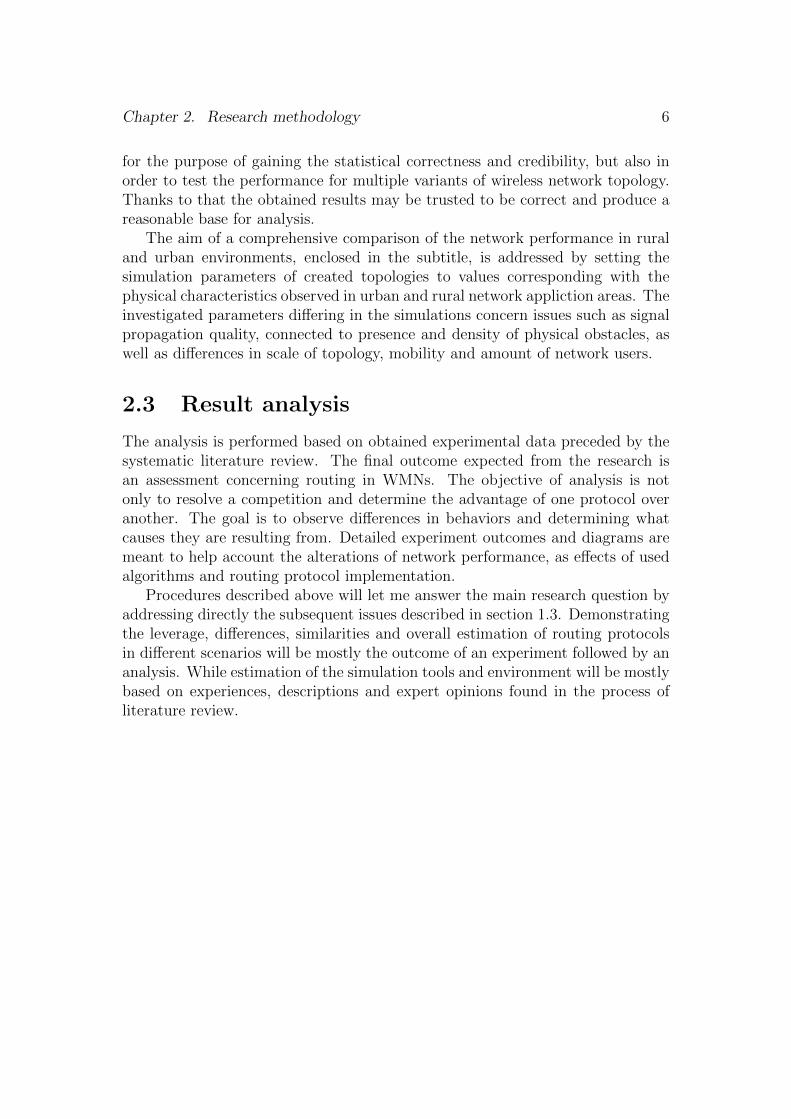
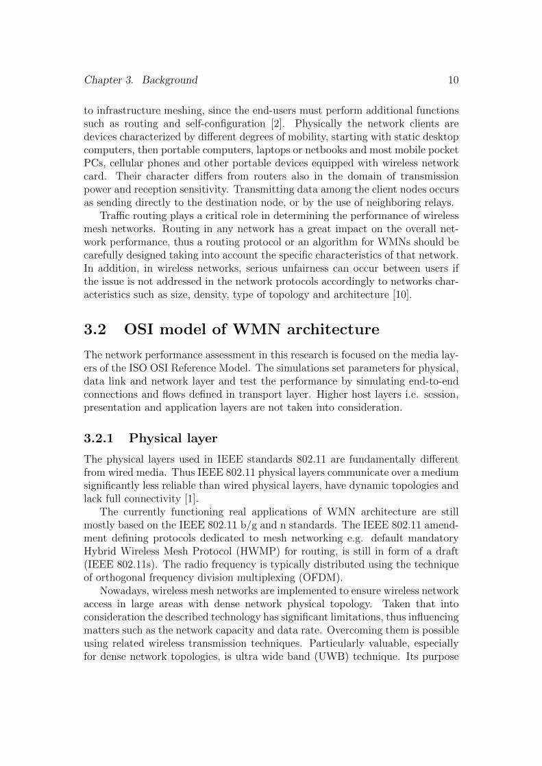
The architecture of WMNs is classified among others, such as hybrid wirelessnetworks, wireless ad hoc networks and wireless sensor networks to a family ofmulti-hop wireless networks [11]. The figure 3.1 shows the relation between thesenetwork architectures.
Figure 3.1: Classification of multi-hop wireless networks [11]
7
Chapter 3. Background 8
Another - internal classification of WMN was proposed by the authors of thepublication A Survey on Wireless Mesh Networks [2]. They divided the WMNarchitectures into three types:
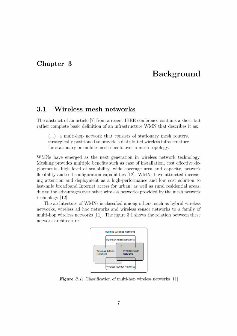
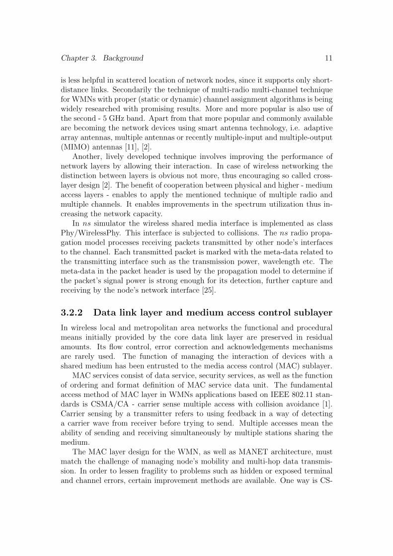
� Infrastructure or Backbone WMNs (figure 3.2) - in this architecture, meshrouters form an infrastructure for clients. The mesh routers form a mesh ofself-configuring, self-healing links among themselves [2].
Figure 3.2: The backbone type of WMN topology
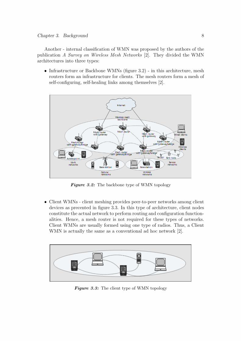
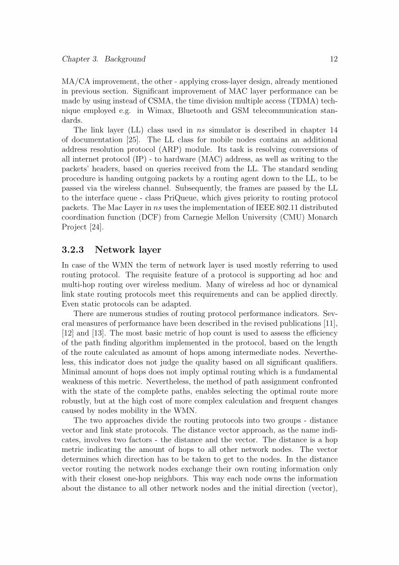
� Client WMNs - client meshing provides peer-to-peer networks among clientdevices as precented in figure 3.3. In this type of architecture, client nodesconstitute the actual network to perform routing and configuration function-alities. Hence, a mesh router is not required for these types of networks.Client WMNs are usually formed using one type of radios. Thus, a ClientWMN is actually the same as a conventional ad hoc network [2].
Figure 3.3: The client type of WMN topology
Chapter 3. Background 9
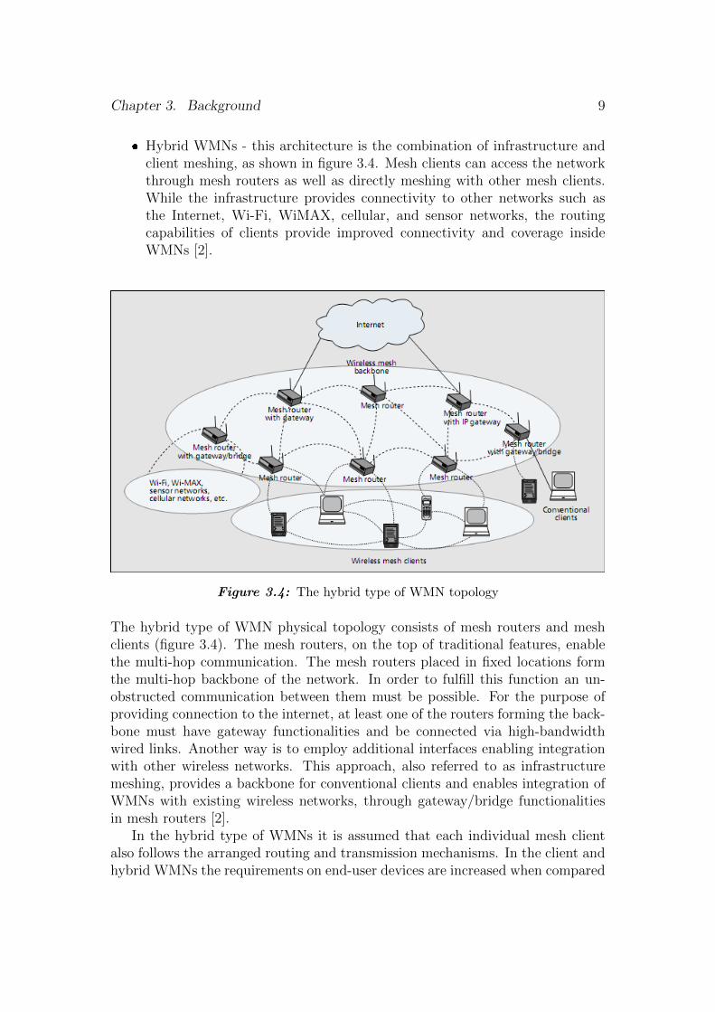
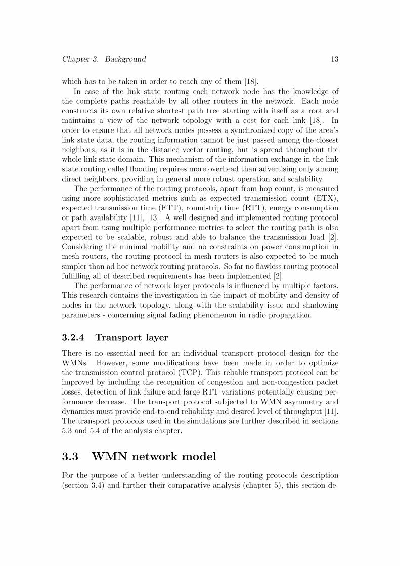
� Hybrid WMNs - this architecture is the combination of infrastructure andclient meshing, as shown in figure 3.4. Mesh clients can access the networkthrough mesh routers as well as directly meshing with other mesh clients.While the infrastructure provides connectivity to other networks such asthe Internet, Wi-Fi, WiMAX, cellular, and sensor networks, the routingcapabilities of clients provide improved connectivity and coverage insideWMNs [2].
Figure 3.4: The hybrid type of WMN topology
The hybrid type of WMN physical topology consists of mesh routers and meshclients (figure 3.4). The mesh routers, on the top of traditional features, enablethe multi-hop communication. The mesh routers placed in fixed locations formthe multi-hop backbone of the network. In order to fulfill this function an un-obstructed communication between them must be possible. For the purpose ofproviding connection to the internet, at least one of the routers forming the back-bone must have gateway functionalities and be connected via high-bandwidthwired links. Another way is to employ additional interfaces enabling integrationwith other wireless networks. This approach, also referred to as infrastructuremeshing, provides a backbone for conventional clients and enables integration ofWMNs with existing wireless networks, through gateway/bridge functionalitiesin mesh routers [2].
In the hybrid type of WMNs it is assumed that each individual mesh clientalso follows the arranged routing and transmission mechanisms. In the client andhybrid WMNs the requirements on end-user devices are increased when compared
Chapter 3. Background 10
to infrastructure meshing, since the end-users must perform additional functionssuch as routing and self-configuration [2]. Physically the network clients aredevices characterized by different degrees of mobility, starting with static desktopcomputers, then portable computers, laptops or netbooks and most mobile pocketPCs, cellular phones and other portable devices equipped with wireless networkcard. Their character differs from routers also in the domain of transmissionpower and reception sensitivity. Transmitting data among the client nodes occursas sending directly to the destination node, or by the use of neighboring relays.
Traffic routing plays a critical role in determining the performance of wirelessmesh networks. Routing in any network has a great impact on the overall net-work performance, thus a routing protocol or an algorithm for WMNs should becarefully designed taking into account the specific characteristics of that network.In addition, in wireless networks, serious unfairness can occur between users ifthe issue is not addressed in the network protocols accordingly to networks char-acteristics such as size, density, type of topology and architecture [10].
3.2 OSI model of WMN architecture
The network performance assessment in this research is focused on the media lay-ers of the ISO OSI Reference Model. The simulations set parameters for physical,data link and network layer and test the performance by simulating end-to-endconnections and flows defined in transport layer. Higher host layers i.e. session,presentation and application layers are not taken into consideration.
3.2.1 Physical layer
The physical layers used in IEEE standards 802.11 are fundamentally differentfrom wired media. Thus IEEE 802.11 physical layers communicate over a mediumsignificantly less reliable than wired physical layers, have dynamic topologies andlack full connectivity [1].
The currently functioning real applications of WMN architecture are stillmostly based on the IEEE 802.11 b/g and n standards. The IEEE 802.11 amend-ment defining protocols dedicated to mesh networking e.g. default mandatoryHybrid Wireless Mesh Protocol (HWMP) for routing, is still in form of a draft(IEEE 802.11s). The radio frequency is typically distributed using the techniqueof orthogonal frequency division multiplexing (OFDM).
Nowadays, wireless mesh networks are implemented to ensure wireless networkaccess in large areas with dense network physical topology. Taken that intoconsideration the described technology has significant limitations, thus influencingmatters such as the network capacity and data rate. Overcoming them is possibleusing related wireless transmission techniques. Particularly valuable, especiallyfor dense network topologies, is ultra wide band (UWB) technique. Its purpose
Chapter 3. Background 11
is less helpful in scattered location of network nodes, since it supports only short-distance links. Secondarily the technique of multi-radio multi-channel techniquefor WMNs with proper (static or dynamic) channel assignment algorithms is beingwidely researched with promising results. More and more popular is also use ofthe second - 5 GHz band. Apart from that more popular and commonly availableare becoming the network devices using smart antenna technology, i.e. adaptivearray antennas, multiple antennas or recently multiple-input and multiple-output(MIMO) antennas [11], [2].
Another, lively developed technique involves improving the performance ofnetwork layers by allowing their interaction. In case of wireless networking thedistinction between layers is obvious not more, thus encouraging so called cross-layer design [2]. The benefit of cooperation between physical and higher - mediumaccess layers - enables to apply the mentioned technique of multiple radio andmultiple channels. It enables improvements in the spectrum utilization thus in-creasing the network capacity.
In ns simulator the wireless shared media interface is implemented as classPhy/WirelessPhy. This interface is subjected to collisions. The ns radio propa-gation model processes receiving packets transmitted by other node’s interfacesto the channel. Each transmitted packet is marked with the meta-data related tothe transmitting interface such as the transmission power, wavelength etc. Themeta-data in the packet header is used by the propagation model to determine ifthe packet’s signal power is strong enough for its detection, further capture andreceiving by the node’s network interface [25].
3.2.2 Data link layer and medium access control sublayer
In wireless local and metropolitan area networks the functional and proceduralmeans initially provided by the core data link layer are preserved in residualamounts. Its flow control, error correction and acknowledgements mechanismsare rarely used. The function of managing the interaction of devices with ashared medium has been entrusted to the media access control (MAC) sublayer.
MAC services consist of data service, security services, as well as the functionof ordering and format definition of MAC service data unit. The fundamentalaccess method of MAC layer in WMNs applications based on IEEE 802.11 stan-dards is CSMA/CA - carrier sense multiple access with collision avoidance [1].Carrier sensing by a transmitter refers to using feedback in a way of detectinga carrier wave from receiver before trying to send. Multiple accesses mean theability of sending and receiving simultaneously by multiple stations sharing themedium.
The MAC layer design for the WMN, as well as MANET architecture, mustmatch the challenge of managing node’s mobility and multi-hop data transmis-sion. In order to lessen fragility to problems such as hidden or exposed terminaland channel errors, certain improvement methods are available. One way is CS-
Chapter 3. Background 12
MA/CA improvement, the other - applying cross-layer design, already mentionedin previous section. Significant improvement of MAC layer performance can bemade by using instead of CSMA, the time division multiple access (TDMA) tech-nique employed e.g. in Wimax, Bluetooth and GSM telecommunication stan-dards.
The link layer (LL) class used in ns simulator is described in chapter 14of documentation [25]. The LL class for mobile nodes contains an additionaladdress resolution protocol (ARP) module. Its task is resolving conversions ofall internet protocol (IP) - to hardware (MAC) address, as well as writing to thepackets’ headers, based on queries received from the LL. The standard sendingprocedure is handing outgoing packets by a routing agent down to the LL, to bepassed via the wireless channel. Subsequently, the frames are passed by the LLto the interface queue - class PriQueue, which gives priority to routing protocolpackets. The Mac Layer in ns uses the implementation of IEEE 802.11 distributedcoordination function (DCF) from Carnegie Mellon University (CMU) MonarchProject [24].
3.2.3 Network layer
In case of the WMN the term of network layer is used mostly referring to usedrouting protocol. The requisite feature of a protocol is supporting ad hoc andmulti-hop routing over wireless medium. Many of wireless ad hoc or dynamicallink state routing protocols meet this requirements and can be applied directly.Even static protocols can be adapted.
There are numerous studies of routing protocol performance indicators. Sev-eral measures of performance have been described in the revised publications [11],[12] and [13]. The most basic metric of hop count is used to assess the efficiencyof the path finding algorithm implemented in the protocol, based on the lengthof the route calculated as amount of hops among intermediate nodes. Neverthe-less, this indicator does not judge the quality based on all significant qualifiers.Minimal amount of hops does not imply optimal routing which is a fundamentalweakness of this metric. Nevertheless, the method of path assignment confrontedwith the state of the complete paths, enables selecting the optimal route morerobustly, but at the high cost of more complex calculation and frequent changescaused by nodes mobility in the WMN.
The two approaches divide the routing protocols into two groups - distancevector and link state protocols. The distance vector approach, as the name indi-cates, involves two factors - the distance and the vector. The distance is a hopmetric indicating the amount of hops to all other network nodes. The vectordetermines which direction has to be taken to get to the nodes. In the distancevector routing the network nodes exchange their own routing information onlywith their closest one-hop neighbors. This way each node owns the informationabout the distance to all other network nodes and the initial direction (vector),
Chapter 3. Background 13
which has to be taken in order to reach any of them [18].In case of the link state routing each network node has the knowledge of
the complete paths reachable by all other routers in the network. Each nodeconstructs its own relative shortest path tree starting with itself as a root andmaintains a view of the network topology with a cost for each link [18]. Inorder to ensure that all network nodes possess a synchronized copy of the area’slink state data, the routing information cannot be just passed among the closestneighbors, as it is in the distance vector routing, but is spread throughout thewhole link state domain. This mechanism of the information exchange in the linkstate routing called flooding requires more overhead than advertising only amongdirect neighbors, providing in general more robust operation and scalability.
The performance of the routing protocols, apart from hop count, is measuredusing more sophisticated metrics such as expected transmission count (ETX),expected transmission time (ETT), round-trip time (RTT), energy consumptionor path availability [11], [13]. A well designed and implemented routing protocolapart from using multiple performance metrics to select the routing path is alsoexpected to be scalable, robust and able to balance the transmission load [2].Considering the minimal mobility and no constraints on power consumption inmesh routers, the routing protocol in mesh routers is also expected to be muchsimpler than ad hoc network routing protocols. So far no flawless routing protocolfulfilling all of described requirements has been implemented [2].
The performance of network layer protocols is influenced by multiple factors.This research contains the investigation in the impact of mobility and density ofnodes in the network topology, along with the scalability issue and shadowingparameters - concerning signal fading phenomenon in radio propagation.
3.2.4 Transport layer
There is no essential need for an individual transport protocol design for theWMNs. However, some modifications have been made in order to optimizethe transmission control protocol (TCP). This reliable transport protocol can beimproved by including the recognition of congestion and non-congestion packetlosses, detection of link failure and large RTT variations potentially causing per-formance decrease. The transport protocol subjected to WMN asymmetry anddynamics must provide end-to-end reliability and desired level of throughput [11].The transport protocols used in the simulations are further described in sections5.3 and 5.4 of the analysis chapter.
3.3 WMN network model
For the purpose of a better understanding of the routing protocols description(section 3.4) and further their comparative analysis (chapter 5), this section de-
Chapter 3. Background 14
fines the model of WMN from a perspective of the network layer. The descriptionis analogical to notation and assumptions presented by Park and Corson [16].
The WMN model is assumed as a graph G = (N,L), where N is a finite set ofnodes and L is a set of initially undirected links. Each node i, j ∈ N is assumedto have a unique node identifier, and each link (i, j) ∈ L is assumed to allowtwo-way communication (i.e. nodes connected by a link can communicate witheach other in either direction). Due to the mobility of the nodes, the set of links Lis changing with time (i.e. new links can be established and existing links can besevered). From the perspective of neighboring nodes, a node failure is equivalentto severing all links incident to that node.
Each initially undirected link (i, j) ∈ L may subsequently be assigned one ofthree states; 1 undirected, 2 directed from node i to node j, or 3 directed fromnode j to node i. If a link (i, j) ∈ L is directed from node i to node j, node iis said to be upstream from node j while node j is said to be downstream fromnode i.
For each node i, there is a group of neighbors of i, Ni ⊆ N , to be the set ofnodes j such that (i, j) ∈ L. The node’s awareness of its neighborhood in set Nis implemented by a link-level protocol. On the network level it is assumed thatall transmitted packets are received correctly and in order of transmission.
Since existing networks of this type typically employ omnidirectional antennas,it is assumed that when a node i transmits a packet, it is broadcasted to all ofits neighbors in the set Ni ⊆ N [16].
3.4 Routing in WMN
The chosen group of routing protocols used in WMNs is investigated and pre-sented based mostly on their individual documentation files acquired from re-liable sources such as Request for Comments (RFC) published by the InternetEngineering Task Force (IETF) [5], [17], [15], IEEE documentation [9], otherdocumentation and articles [14], [21], [18], [28].
3.4.1 DSDV
The Highly Dynamic Destination-Sequenced Distance Vector Routing (DSDV) ishistorically the first of investigated routing protocols, defined first in August of1994. As described in previous section 3.3, an ad hoc network is the cooperativeengagement of a collection of mobile hosts without the required intervention ofany centralized Access Point. The DSDV routing protocol operates on such ad hocnetworks. It specifies each mobile host as a specialized router, which periodicallyadvertises its view of the interconnection topology with other mobile hosts withinthe network [28].
Chapter 3. Background 15
DSDV construction is based on a modification of the basic Bellman Ford(BF) routing mechanisms, as specified by routing information protocol (RIP),to make it suitable for a dynamic and self-starting network mechanism as isrequired by users wishing to utilize ad hoc networks [18]. The modificationsaddress the drawbacks of BF, related to the poor counting to infinity propertiyof such algorithms in the face of broken links and the resulting time dependentnature of the interconnection topology describing the links between the mobilehosts.
DSDV models the mobile nodes as routers, which are cooperating to forwardpackets as needed to each other using the wireless broadcast medium. The in-formation in the routing tables is similar to routing tables with distance vector(BF) algorithms, but includes a sequence number, as well as settling-time data,useful for damping out fluctuations in route table updates.
The routing information is advertised by broadcasting or multicasting thepackets which are transmitted periodically and incrementally as topological changesare detected - for instance, when stations move within the network. Data is alsokept about the length of time between arrival of the first and the arrival of the bestroute for each particular destination. Based on this data it is possible to identifyroutes which are about to change soon. The advertisement of routes which maynot be stable is delayed in order to reduce the number of rebroadcasts. In casewhen a link has been broken the link is described by an∞ metric and a sequencenumber which cannot be correctly generated by any destination node [18].
The DSDV protocol requires each mobile station to advertise, to each of itscurrent neighbors, its own routing table (for instance, by broadcasting its entries).The entries in this list may change fairly dynamically over time, so the advertise-ment must be made often enough to ensure that every mobile node can almostalways locate every other mobile node of the collection. In addition, each mobilenode agrees to relay data packets to other nodes upon request. This agreementputs an emphasis on the ability to determine the shortest number of hops for aroute to a destination.
The DSDV implementation borrows from BF the existing mechanism of trig-gered updates to make sure that pertinent route table changes can be propagatedthroughout the population of mobile hosts as quickly as possible whenever anytopology changes are noticed. This includes movement from place to place as wellas the disappearance of a mobile host from the interconnect topology e.g. as aresult of turning off its power [18], [28].
The DSDV route tables are separated into two distinct structures in orderto combat problems arising with large populations of mobile hosts, which cancause route updates to be received in an order delaying the best metrics untilafter poorer metric routes are received. The actual routing is done according toinformation kept in the internal route table, but this information is not alwaysadvertised immediately upon receipt. An additional mechanism based upon re-cent history regulates the time of advertising a host change when it is likely, that
Chapter 3. Background 16
it is stable.One of the most important parameters to be chosen is the time between broad-
casting the routing information packets. All the nodes interoperating to createdata paths between themselves broadcast the necessary data periodically, onceevery few seconds. In a wireless medium, it is important to keep in mind thatbroadcasts are limited in range by the physical characteristics of the medium.The data broadcasted by each mobile node will contain its new sequence numberand the following information for each new route:
� the destination’s address;
� the number of hops required to reach the destination;
� the sequence number of the information received regarding that destination,as originally stamped by the destination.
In case of a new or substantially modified route information is received itis retransmitted soon, effecting the most rapid possible dissemination of routinginformation among all the cooperating mobile nodes. This quick re-broadcastintroduces a new requirement for our protocols to converge as soon as possible.It would be calamitous if the movement of a mobile host caused a storm ofbroadcasts, degrading the availability of the wireless medium.
A broken link event frequent in WMNs may be detected by the layer-2 proto-col, or it may instead be inferred if no broadcasts have been received for a whilefrom a former neighbor. A broken link is described by a metric of ∞ (i.e., anyvalue greater than the maximum allowed metric). When a link to a next hop hasbroken, any route through that next hop is immediately assigned an ∞ metricand assigned an updated sequence number. Since this qualifies as a substantialroute change, such modified routes are immediately disclosed in a broadcast rout-ing information packet. Building information to describe broken links is the onlysituation when the sequence number is generated by any mobile host other thanthe destination host.
In a very large population of mobile nodes, time between broadcasts of therouting information packets must be adjusted. In order to reduce the amount oftransmitted data there are two types of packets carrying routing information. Onecarries all available routing information - full dump, the other - only informationchanged since the last full dump incremental. Full dumps can be transmittedrelatively infrequently when no movement of mobile nodes is occurring. In caseof intensive movement, the rising size of an incremental can be decreased by ascheduled full dump [18].
There are significant limitations of routing in the DSDV protocol i.e. it pro-vides only a single path between each given source and destination pair [16].Furthermore, the protocol’s performance is highly dependent on selected param-eters of periodic update interval, maximum value of the “settling time” for a
Chapter 3. Background 17
destination and the number of update intervals which may transpire before aroute is considered stable. It is difficult to assess the impact that selection ofthese parameters has on performance, but the parameter selection appears to becritical. These parameters very likely represent a trade-off between the latencyof valid routing information and excessive communication overhead. To furthercomplicate the problem, an optimal parameter selection is dependent on the net-working environment (i.e. the size of the network, rate of topological change,etc.) [16].
3.4.2 AODV
The Ad hoc On-Demand Distance Vector (AODV) routing protocol offers anability of quick adaptation to dynamic link conditions, low processing and memoryoverhead, low network utilization, and determines unicast routes to destinationswithin the ad hoc network. It uses destination sequence numbers to ensure theelimination of loops, and consequently the counting to infinity problem, at alltimes, thus avoiding related problems associated with classical distance vectorprotocols [17].
The Ad hoc On-Demand Distance Vector (AODV) algorithm:
� enables dynamic, self-starting, multi-hop routing between participating mo-bile nodes wishing to establish and maintain an ad hoc network;
� allows mobile nodes to obtain routes quickly for new destinations, and doesnot require nodes to maintain routes to destinations that are not in activecommunication;
� allows mobile nodes to respond to link breakages and changes in networktopology in a timely manner;
� offers quick convergence when the ad hoc network topology changes byavoiding the BF “counting to infinity” problem [28];
� notifies the affected set of nodes in case of a broken link, enabling them toinvalidate the routes using the lost link information [17].
A feature similar for AODV and DSDV is the use of a destination sequencenumber for each route entry. The destination sequence number is created by thedestination to be included along with any route information it sends to requestingnodes. This way AODV eliminates the problem of counting to infinity at the sametime not affecting the implementation simplicity. The choice between possibleroutes to a destination is made by selecting the greatest sequence number.
AODV defines the following routing messages: Route Requests (RREQs),Route Replies (RREPs), and Route Errors (RERRs). The amount of forwardedmessages is controlled by limiting the IP broadcast address to 255.255.255.255.
Chapter 3. Background 18
The AODV operations require certain messages i.e. RREQ to be disseminatedamong the whole network. The range of dissemination of such RREQ messagesis indicated by the TTL field in the IP header [17].
The on-demand character of protocol implies that as long as the endpoints ofa communication connection have valid routes to each other, no routing messagesneed to be sent. In case of the need for a route modification, the source nodebroadcasts a RREQ message to find a route to the desired destination. A routedetermination is completed when the RREQ message reaches either the destina-tion itself, or an intermediate node with defined route to the destination. Theroute of an intermediate node can be used conditionally if its associated sequencenumber is equal or greater than in the RREQ. In this case the information abouta new rout is passed to the original source by a unicast RREP message tracingback the route crossed by a packet containing RREQ message.
The RERR message is used to notify other nodes in case when a node discov-ers a broken link among the monitored neighbors in active routes. The RERRmessage indentifies the destinations which are no longer reachable as a result ofthe broken link. Reporting these changes by network nodes is possible thanks toso called node’s precursor list containing the IP address of all node’s neighborsthat are likely to use it as a next hop [17].
The routing information, analogically to DSDV, is kept in route tables. Itstores entries for all, even short-lived routes, which are created to temporarilystore reverse paths towards nodes originating RREQs. The data kept in eachrouting table entry is also partially analogical to DSDV (i.e. in destination IPaddress and sequence number, hop count or next hop). Among the supplementaryfields are the valid destination sequence number flag and the list of precursors.
The AODV routing protocol is designed for mobile ad hoc networks topologieswith population of tens to thousands mobile nodes. It handles low, moderate,and relatively high mobility rates, as well as a variety of data traffic levels [17].AODV is designed for use in networks where the nodes can all trust each other,either by use of preconfigured keys, or based on known fact of no malicious nodes.It has been designed to reduce the dissemination of control traffic and eliminateoverhead on data traffic, in order to improve wireless network’s scalability andperformance.
3.4.3 OLSR
The Optimized Link State Routing protocol or short OLSR is a routing proto-col that was developed by the Internet Engineering Task Force (IETF) and isspecified in the RFC 3626 [5]. As the name suggests it is an advanced versionof the well-known wired Link State Routing (LSR) algorithm. However, OLSRwas specifically designed to serve the particular needs of mobile ad hoc networks(MANET). Therefore, it inherits many characteristics of its predecessor, but dif-fers from it in important details. The main adjustments that were made tackle
Chapter 3. Background 19
the reduction of administrative data exchange in favor to avoid signal collisions aswell as increase the overall protocol performance [5]. To enable the reader to un-derstand the previously mentioned similarities and differences between the classicLink State algorithm and OLSR, as well as help understanding the protocol itself,a brief overview about the functioning is presented in the next paragraphs.
Each node in an OLSR network possesses, just like in LSR, a complete rep-resentation of the whole network topology and maintains this information on aperiodic regular basis by exchanging topology information with other nodes. Thismakes OLSR a member of the proactive routing algorithms family. The previ-ously mentioned information interchange is done in OLSR by the means of twospecific messages the so called HELLO and Topology Control (TC) messages [5].The former type is utilized similar to LSR to sense the links to other nodes in thedirect neighborhood. Speaking in terms of OLSR this means at first all one-hopand subsequently all two-hop neighbors. Using the responses of the other nodesand a specific algorithm each individual node is able to select for itself a subsetout of the other nodes which are from then on referred to as Multipoint Relays(MPRs). Their task is to execute the flooding as well as manage their parts ofthe topology as it was formerly done in LSR by all nodes. Therefore, each of theMPRs sends TC-messages containing local topology information to their respec-tive MPRs while forwarding received topology information - foreign TC messages- to their Multipoint Relay selectors [5]. This ensures that routing informationis still distributed throughout the whole network while limiting the flooding dataoverhead only to specific nodes - namely the MPRs. Moreover, due to the factthat MPRs selected in a way that the all nodes in the network are covered, thedenser the network becomes the less Multipoint Relays are required. Hence thislowers the administrative data exchange and allows a good scalability regardingthe network size and density.
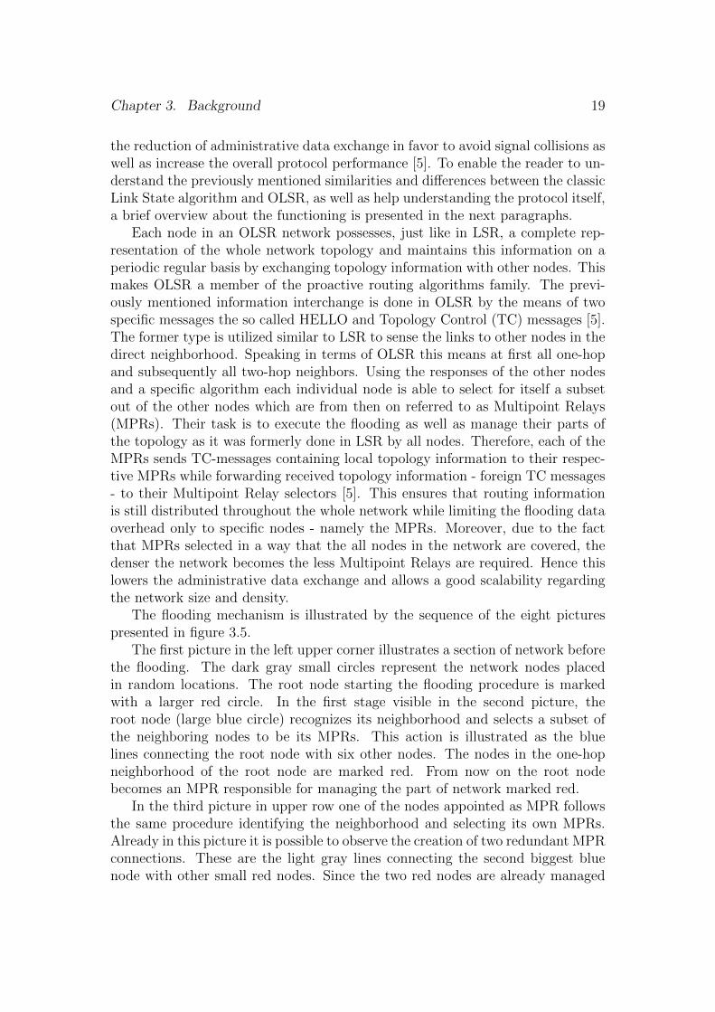
The flooding mechanism is illustrated by the sequence of the eight picturespresented in figure 3.5.
The first picture in the left upper corner illustrates a section of network beforethe flooding. The dark gray small circles represent the network nodes placedin random locations. The root node starting the flooding procedure is markedwith a larger red circle. In the first stage visible in the second picture, theroot node (large blue circle) recognizes its neighborhood and selects a subset ofthe neighboring nodes to be its MPRs. This action is illustrated as the bluelines connecting the root node with six other nodes. The nodes in the one-hopneighborhood of the root node are marked red. From now on the root nodebecomes an MPR responsible for managing the part of network marked red.
In the third picture in upper row one of the nodes appointed as MPR followsthe same procedure identifying the neighborhood and selecting its own MPRs.Already in this picture it is possible to observe the creation of two redundant MPRconnections. These are the light gray lines connecting the second biggest bluenode with other small red nodes. Since the two red nodes are already managed

Chapter 3. Background 20
Figure 3.5: The mechanism of MPR flooding in the OLSR protocol
by another MPR, no new connection is needed. The last picture in the upperrow and the first two pictures in the lower row present the next stages of MPRflooding. More and more MPRs are assigned and also more redundant connectionsare formed.
The third picture in the lower row presents the stage in which appointing theMPRs is completed and every network node (small red circles) has a MPR nodein its direct neighborhood. This is the stage when the redundant connections areremoved, which may be observed in this picture as disappearing light grey lines.The last picture in the right lower corner presents the result of the flooding. Thereare no dark grey circles representing nodes omitted by the routing mechanism.The plain nodes are marked as red circles and the MPRs as larger blue circles. Allthe MPRs are connected in a net assuring complete routing information exchange.Each of the MPR will pass the routing information to its MPRs - neighbors anddisseminate the updated information among its closest neighbors.
OLSR, although it is still a young protocol, offers already a vast number ofimplementations that can be found throughout the Internet. Moreover, it al-ready passed the stage of being just a theoretical idea by virtue of being alreadyused as the major routing protocol by for instance the Freie Funknetze in Berlin,Germany. However, lately OLSR was criticized because of its large energy con-sumption due to constant data exchange and large topology databases.
Chapter 3. Background 21
3.4.4 TORA
The Temporally-Ordered Routing Algorithm (TORA) is the outcome of researchconducted by Vincent Park and Scott Corson in a cooperative project betweenthe Naval Research Laboratories, USA and the University of Maryland, USA in1997. Both of them published TORA later in 2001 as an Internet draft whichexpired after six months [15]. The routing algorithm itself bases heavily on twoothers Gafni-Bertsekas [16] (GB) as well as Lightweight Mobile Routing (LMR)algorithm [15]. Its fundamental improvement is quicker convergence in partitionednet.
The algorithm implemented in TORA is distributed in that nodes need onlymaintain information about adjacent nodes (i.e. one-hop knowledge) [15]. Ituses the unique graph mechanism of route creation and maintenance using ametric called the height of the node. The information can only be passed indirection from higher to lower nodes. It guarantees that all routes are loop-free, and typically provides multiple routes for any source-destination pair whichrequires a route [15]. Like LMR, the protocol is source initiated and quicklycreates a set of routes to a given destination only when desired. Since multipleroutes are typically established, many topological changes require no reaction atall as having a single route is sufficient. Following topological changes whichdo require reaction, the protocol quickly reestablishes valid routes. This abilityto initiate and react infrequently serves to minimize communication overhead.Finally, in the event of a network partition, the protocol detects the partitionand erases all invalid routes within a finite time.
3.4.5 HWMP
The Hybrid Wireless Mesh Protocol (HWMP) is a mesh routing protocol thatcombines the flexibility of on-demand routing with proactive topology tree ex-tensions. The reactive and proactive elements of HWMP are combined in orderto enable optimal and efficient path selection in a wide variety of mesh networks(with or without infrastructure).
HWMP uses a common set of protocol primitives, generation and processingrules taken from Ad Hoc On-Demand (AODV) routing protocol (subsection 3.4.2)adapted for Layer-2 address-based routing and link metric awareness. AODVforms the basis for finding on-demand routes within a mesh network while addi-tional primitives are used to proactively set up a distance vector tree rooted at asingle root mesh node. The root role that enables building of topology tree is aconfigurable option of a mesh node [9].
HWMP supports two modes of operation depending on the configuration.These modes are:
Chapter 3. Background 22
� On-demand mode: this mode allows mesh nodes to communicate using peer-to-peer routes. It is used in situations where there is no root configured. Itis also used in certain circumstances if there is a root configured.
� Proactive tree building mode: this can be performed by using either theRREQ or RANN mechanism.
These modes are not exclusive: on-demand and proactive modes may be usedsimultaneously.
All HWMP modes of operation utilize common processing rules and primi-tives. HWMP control messages are the Route Request (RREQ), Route Reply(RREP), Route Error (RERR) and Root Announcement (RANN). The metriccost of the links determines which routes HWMP builds. In order to propa-gate the metric information between mesh nodes, a metric field is used in theRREQ, RREP and RANN messages [9]. Routing in HWMP uses a sequencenumber mechanism to maintain loop-free connectivity at all times. Each meshnode maintains its own sequence number, which is propagated to other meshnodes in the HWMP control messages.
Chapter 4
Simulation modeling
The matter of measurable differences between applications of WMNs in differentresidential areas has been often mentioned, but hardly addressed so far. Thereis a need for revision and evaluation of network performance depending on typeof used routing protocol in residential areas of different density. As the answerto that need in this work the performance of chosen routing protocols for WMNsis evaluated in scenarios imitating varying conditions of network topologies fromrural to urban residential areas. Performance is evaluated by the means of multi-stage simulations with respect to metrics such as: packet delivery ratio, averageend to end packet delay, normalized routing load and network throughput. Theexperiment is performed by the use of Network Simulator ns (licensed for useunder version 2 of the GNU General Public License) to compare the group ofchosen routing protocols representing specific approaches and algorithms. Thechoice of this simulator is motivated by its many advantages, among which are:open source code, rich amount of implemented protocols and contributed code,reliability confirmed by common usage for research purposes. The simulationsresults provide the base for evaluation of efficiency and performance comparisonof routing protocols.
4.1 The ns simulator
The core tool for performing simulations is the ns network simulator, sometimesalso referd to as ns-2. ns is a simulator, written in the object oriented program-ming language C++, with an OTcl interpreter as a frontend.
The implementation structure of the network simulator ns is somewhat unique.The simulator supports two hierarchies, which are closely related to each other: aclass hierarchy in C++ and a similar class hierarchy within the OTcl interpreter.New simulator objects are created through the interpreter. These objects areinstantiated within the interpreter, and are closely mirrored by a correspondingobject in the compiled class hierarchy in C++ [25]. The benefits of this dual-ity are flexibility needed for frequent modifications of simulation configurationand high efficiency (run-time speed) essential for uses such as detailed protocolimplementation.
23

Chapter 4. Simulation modeling 24
Setting up a simulation starts with creating an instance of the OTcl classSimulator and calling various methods to create topologies, add nodes, and con-figure other aspects of the simulation. Each simulation requires a single instanceof the class Simulator to control and operate that simulation. The class providesinstance procedures to create and manage the topology, and internally storesreferences to each element of the topology.
An ns simulation is driven by an event scheduler that defaults to a calendarscheduler [25]. When a new simulation object is created using the OTcl in-terpreter, the initialization procedure performs operations which involve amongother secondary actions defining the packet format, creating the previously men-tioned scheduler and an entity named null agent. The roles of packet formatinitialization and the scheduler are self-explanatory, whereas task of a null agentmight not be obvious. It functions as a discard sink and is generally used fordropped packets or as a destination for packets that are not counted or recorded.
Having set the essentials for starting a simulation, the next matter of concernis creating a scenario. This involves defining a topology and assigning nodes. Thetopology’s basics are characterized by its width and length, whereas the propertiesof an individual ns node are more complex. A node is essentially represented by acollection of classifiers which are i.e. control functions, address and port numbermanagement, unicast routing functions, agent management and assigned links toneighbors [25]. For wired and wireless nodes the configuration requires, as onewould expect, different classifiers. A mobile node is the basic node object withadded functionalities of a wireless and mobile node such as capability of movingwithin a given topology or ability to receive and transmit signals to and from awireless channel. A major difference between them is that a mobile node is notconnected by means of links to other nodes or mobile nodes. These qualities ofa network node enable simulations of wireless LAN, multi-hop ad hoc networksand meshing.
One can configure a mobile node with desired values for ad hoc-routing pro-tocol, network stack, channel, topography, propagation model, optional usage ofwired routing and packet tracing at different levels (router, MAC, agent). Whencreating a mobile node one can make use of standard API for OTcl simulationscripts, which is presented in various examples within the ns documentation [25].
What is expected from the described tool is the simulation of communicationbetween the nodes spread across the topology. Simulating the phenomenon ofsending, forwarding and receiving or dropping packets requires predefined end-points where network-layer packets are constructed or consumed. These are repre-sented by agents. Agents are used in the implementation of protocols at differentlayers. In ns one can find support for variety of protocol agents.
Chapter 4. Simulation modeling 25
4.2 Simulation environment
The simulations were performed using most up to date version of ns networksimulator, which is ns 2.34 released on June 17th 2009. The ns is distributed inpackages called ns-allinone, containing along with the simulator, a set of requiredcomponents and optional components. Several of them were used for simulationpurposes such as movement and traffic generation and parameter calculation.
The ns simulator is primarily developed on Unix systems and requires a C++compiler. Running ns in Windows systems involves installing Unix-like environ-ment and command-line interface - e.g. Cygwin [25]. For this reason ns was usedwithin a computer system where it can run natively, namely Ubuntu release 10.10(Maverick Meerkat).
The process of running simulations with desired parameters and subsequentlyperforming analysis of outcomes and sketching diagrams, is regulated by a shellscript. The analysis and diagram creation tools themselves are implemented aspython scripts having ns trace files as input and producing analysis outcomes re-spectively in form of text files and pictures of diagrams in .png format. Diagramsare created using methods of matplotlib packet for python.
4.3 Simulation implementation details
Creating possibly realistic simulation scenarios and mechanisms of a wireless meshnetwork was an important objective of this research. Thus several mechanismsof simulation as well as network properties were investigated in deep in orderto assure meaningful results of conducted experiment. The unique collection ofsimulation settings involves in particular router nodes and mobile network node’sconfiguration, shadowing effect affecting radio propagation and characteristic mo-bility of nodes.
4.3.1 Node’s movement
There is a significant distinction made between mobile and router nodes in simu-lation topologies in order to illustrate real conditions. The main and most visibledifference is lack of movement for router nodes. Mobility of client nodes is gener-ated using a setdest component [25]. It is represented in text form and appendedto simulation as an input source file containing individual node’s movement time,destination and velocity.
Another component of ns-allinone packet - cbrgen.tcl is used for generatingtraffic source files for simulation scenario [25]. This tool is used in a usual manner.The traffic is generated, as mentioned in subsection 5.1, by assigning agents tonodes. The types of used agents are:
� TCP - a “Tahoe” TCP sender;
Chapter 4. Simulation modeling 26
� TCPSink - a “Tahoe” TCP receiver;
� UDP - a basic UDP agent;
� Null - a degenerate agent which discards packets.
4.3.2 Node’s transmission range
Apart from mobility, the router and mobile node’s properties differ in the matterof receiving threshold and transmitting power. The value of receiving threshold(represented by variable RXThresh assigned to network interface type Phy/Wire-lessPhy in OTcl simulation code) is assigned to a wireless node and determinesthe minimum value of packet’s signal power required to succeed with its delivery.If the packet’s signal power at the destination node doesn’t reach the receivingthreshold value, it is marked as error and dropped by the MAC layer. On thesending side of communication, the initial packet signal power is regulated bytransmitting power (Pt in simulation code) [25].
4.3.3 Radio signal propagation
The signal power fluctuates in a way determined by phenomenon of radio wavepropagation [1], which leads us to next issue essential for simulating wireless com-munication, namely radio propagation models. These models are used to predictthe received signal power of each packet. Up to now there are three propagationmodels in ns, which are the free space model, two-ray ground reflection modeland the shadowing model [25].
The free space propagation model assumes the ideal propagation conditionswith a clear line-of-sight between the transmitter and receiver [25]. This modelbasically represents the communication range as a circle around the transmitter.If a receiver is within the circle, it receives all packets. Otherwise, it loses allpackets.
Two-ray ground reflection model gives more accurate prediction at a longdistance than the free space model based on considering both - the direct pathand a ground reflection path. Still, same as the free space propagation model, itpredicts the received power as a deterministic function of distance representingthe communication range as an ideal circle.
Those are the acceptable and commonly used simplifications of radio propa-gation for most of simulation based research. However, an attempt to investigaterealistic conditions requires determining the received power at certain distance bya more complex computation. It is due to multipath propagation effects, whichis also known as fading effects. These are taken in consideration in shadowingpropagation model [25]. This model redefines the calculation of the mean receivedpower at distance making it dependent on the value called path loss exponent,
Chapter 4. Simulation modeling 27
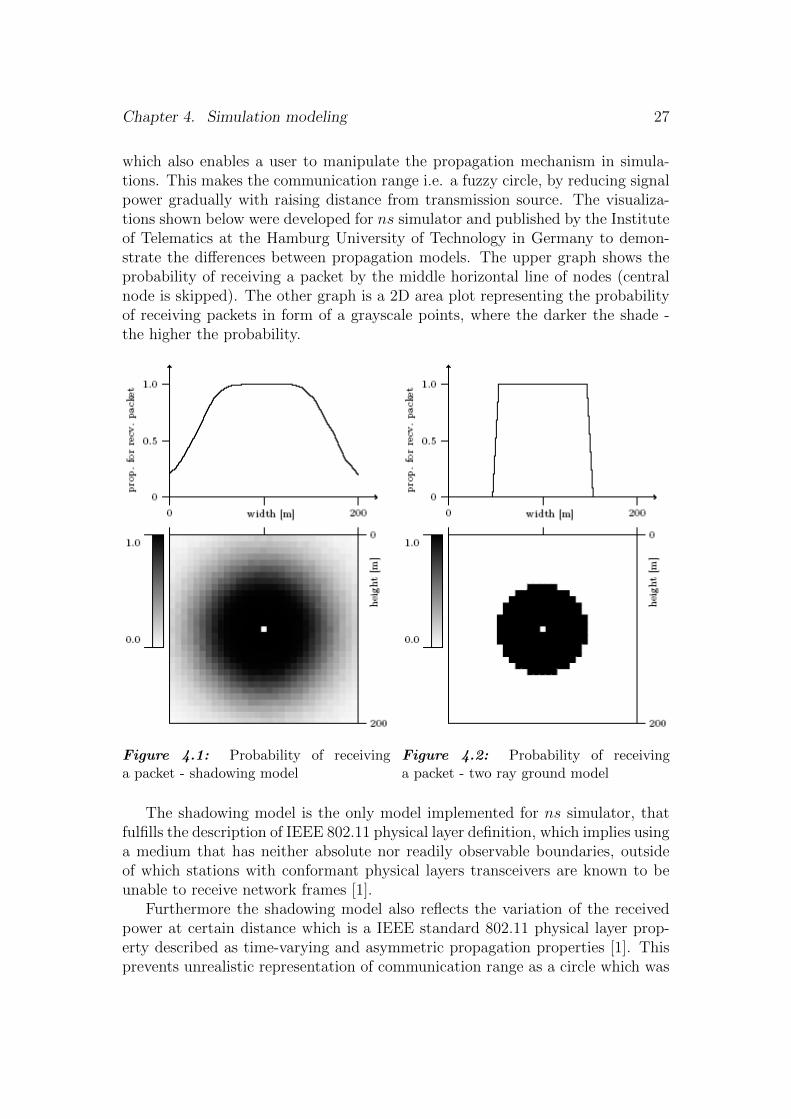
which also enables a user to manipulate the propagation mechanism in simula-tions. This makes the communication range i.e. a fuzzy circle, by reducing signalpower gradually with raising distance from transmission source. The visualiza-tions shown below were developed for ns simulator and published by the Instituteof Telematics at the Hamburg University of Technology in Germany to demon-strate the differences between propagation models. The upper graph shows theprobability of receiving a packet by the middle horizontal line of nodes (centralnode is skipped). The other graph is a 2D area plot representing the probabilityof receiving packets in form of a grayscale points, where the darker the shade -the higher the probability.
Figure 4.1: Probability of receivinga packet - shadowing model
Figure 4.2: Probability of receivinga packet - two ray ground model
The shadowing model is the only model implemented for ns simulator, thatfulfills the description of IEEE 802.11 physical layer definition, which implies usinga medium that has neither absolute nor readily observable boundaries, outsideof which stations with conformant physical layers transceivers are known to beunable to receive network frames [1].
Furthermore the shadowing model also reflects the variation of the receivedpower at certain distance which is a IEEE standard 802.11 physical layer prop-erty described as time-varying and asymmetric propagation properties [1]. Thisprevents unrealistic representation of communication range as a circle which was
Chapter 4. Simulation modeling 28
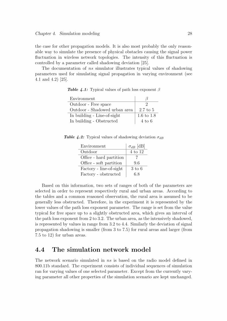
the case for other propagation models. It is also most probably the only reason-able way to simulate the presence of physical obstacles causing the signal powerfluctuation in wireless network topologies. The intensity of this fluctuation iscontrolled by a parameter called shadowing deviation [25].
The documentation of ns simulator illustrates typical values of shadowingparameters used for simulating signal propagation in varying environment (see4.1 and 4.2) [25].
Table 4.1: Typical values of path loss exponent β
Environment βOutdoor - Free space 2Outdoor - Shadowed urban area 2.7 to 5In building - Line-of-sight 1.6 to 1.8In building - Obstructed 4 to 6
Table 4.2: Typical values of shadowing deviation σdB
Environment σdB [dB]Outdoor 4 to 12Office - hard partition 7Office - soft partition 9.6Factory - line-of-sight 3 to 6Factory - obstructed 6.8
Based on this information, two sets of ranges of both of the parameters areselected in order to represent respectively rural and urban areas. According tothe tables and a common reasoned observation, the rural area is assumed to begenerally less obstructed. Therefore, in the experiment it is represented by thelower values of the path loss exponent parameter. The range is set from the valuetypical for free space up to a slightly obstructed area, which gives an interval ofthe path loss exponent from 2 to 3.2. The urban area, as the intensively shadowed,is represented by values in range from 3.2 to 4.4. Similarly the deviation of signalpropagation shadowing is smaller (from 3 to 7.5) for rural areas and larger (from7.5 to 12) for urban areas.
4.4 The simulation network model
The network scenario simulated in ns is based on the radio model defined in800.11b standard. The experiment consists of individual sequences of simulationran for varying values of one selected parameter. Except from the currently vary-ing parameter all other properties of the simulation scenario are kept unchanged.
Chapter 4. Simulation modeling 29
The general default values of a simulation are visible in the listing from the sim-ulation file written in OTcl language, presented below (listing 4.1).
# ==================== ## SET MAIN OPTIONS ## ==================== #
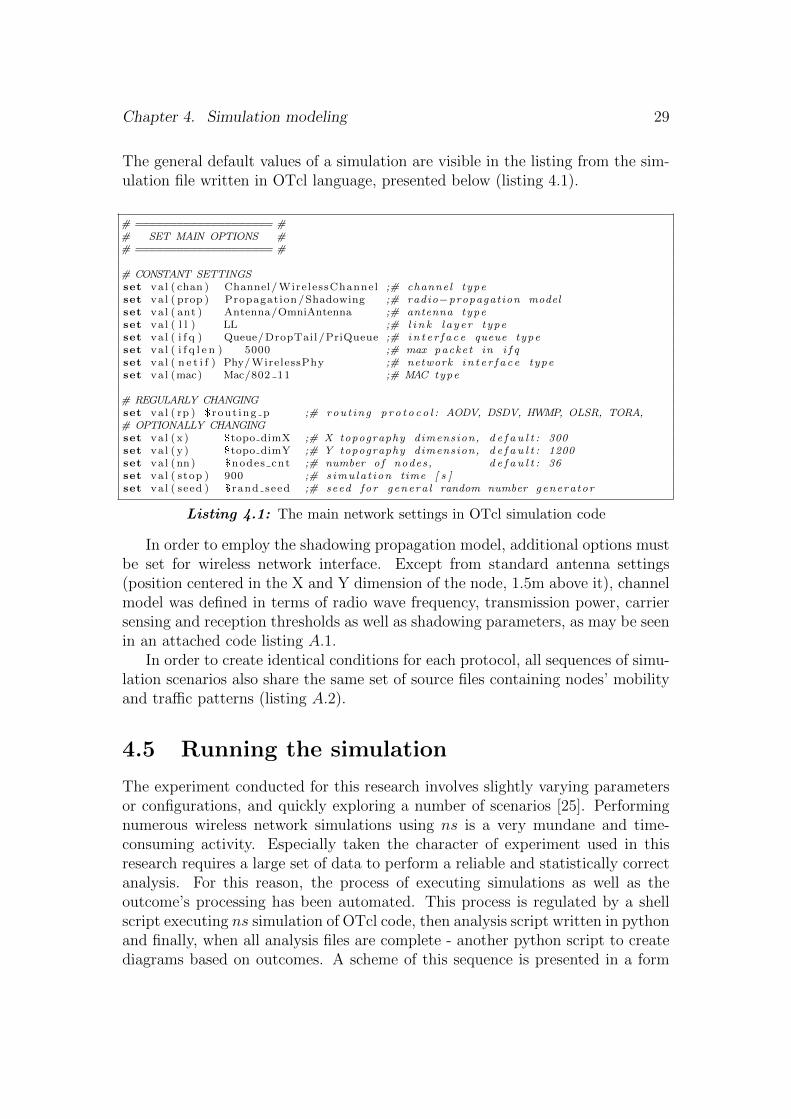
# CONSTANT SETTINGSset va l ( chan ) Channel/Wire lessChannel ;# channel typeset va l ( prop ) Propagation /Shadowing ;# radio−propagation modelset va l ( ant ) Antenna/OmniAntenna ;# antenna typeset va l ( l l ) LL ;# l i n k l a y e r typeset va l ( i f q ) Queue/DropTail /PriQueue ;# i n t e r f a c e queue typeset va l ( i f q l e n ) 5000 ;# max packet in i f qset va l ( n e t i f ) Phy/WirelessPhy ;# network i n t e r f a c e typeset va l (mac) Mac/802 11 ;# MAC type
# REGULARLY CHANGINGset va l ( rp ) $ rout ing p ;# rou t ing p r o t o c o l : AODV, DSDV, HWMP, OLSR, TORA,# OPTIONALLY CHANGINGset va l ( x ) $topo dimX ;# X topography dimension, d e f a u l t : 300set va l ( y ) $topo dimY ;# Y topography dimension, d e f a u l t : 1200set va l (nn) $nodes cnt ;# number o f nodes , d e f a u l t : 36set va l ( stop ) 900 ;# s imu la t ion time [ s ]set va l ( seed ) $ rand seed ;# seed fo r genera l random number generator
Listing 4.1: The main network settings in OTcl simulation code
In order to employ the shadowing propagation model, additional options mustbe set for wireless network interface. Except from standard antenna settings(position centered in the X and Y dimension of the node, 1.5m above it), channelmodel was defined in terms of radio wave frequency, transmission power, carriersensing and reception thresholds as well as shadowing parameters, as may be seenin an attached code listing A.1.
In order to create identical conditions for each protocol, all sequences of simu-lation scenarios also share the same set of source files containing nodes’ mobilityand traffic patterns (listing A.2).
4.5 Running the simulation
The experiment conducted for this research involves slightly varying parametersor configurations, and quickly exploring a number of scenarios [25]. Performingnumerous wireless network simulations using ns is a very mundane and time-consuming activity. Especially taken the character of experiment used in thisresearch requires a large set of data to perform a reliable and statistically correctanalysis. For this reason, the process of executing simulations as well as theoutcome’s processing has been automated. This process is regulated by a shellscript executing ns simulation of OTcl code, then analysis script written in pythonand finally, when all analysis files are complete - another python script to creatediagrams based on outcomes. A scheme of this sequence is presented in a form

Chapter 4. Simulation modeling 30
of diagram (figure 4.3) shown below.
Figure 4.3: BPMN diagram of the simulation running process outline
This diagram specifies the simulating and analysis process using Business Pro-cess Model and Notation (BPMN) graphical representation. The OTcl script re-quires a set of arguments including parameters such as name of simulated routingprotocol, values for shadowing propagation - path loss exponent and shadowingdeviation, dimensions of topology (width and length), number of mobile nodesin the scenario and also number of simulation repeated in the sequence. Exceptfrom the simulation arguments, each simulation uses two external source files.These are the files containing OTcl code for nodes positioning and movement inone, and traffic pattern in the other. Those files are generated using respectivelysetdest and cbrgen.tcl components of ns-allinone packet, which were described inprevious subsection.
Successful simulation writes the progression of succeeding packets into anoutput file called trace file. In order to construe the outcomes of simulation theanalysis python script reads and interprets the content of each trace file. Subse-quently, the values needed to evaluate chosen performance metrics: packet delaytime, throughput, successful deliveries and routing load, are being accumulatedand averaged. This procedure is repeated for the number of trace files equal tonumber of simulation runs in sequence for each routing protocol. Afterwards, theresults for all runs are averaged in order to obtain the statistically correct value,which is then written in text format into an analysis outcomes file.
After completing the set of simulations’ sequences for certain parameter, eachof the analysis files contains a table of values for one of the four metrics whererows refer to changing value of parameter and columns respectively - to routingprotocols. At this moment the diagram creating script is executed. It operates ondata acquired from an analysis file and creates diagram plots using the contentof the table. As diagram’s description i.e. X and Y axis as well as diagram title,the script uses the arguments with which it was called.
Chapter 5
Analysis of the outcomes
The experiment outcomes are mostly fulfilling the expectations. Applying fourof the five chosen protocols returned sensible results with some minor simulationproblems encountered in several cases particularly for OLSR and DSDV proto-cols. The downside is the failure to utilize the TORA - the fifth routing protocol.The version of TORA originally distributed with ns failed to route the packetsand produced large amounts of incongruous packet trace data never managingto conduct complete a full run of a simulation. The alternative versions andmodifications made by patching the original version led to similar results. Forthis reason the TORA algorithm has been excluded from the analysis. In thischapter the four routing protocols: DSDV, AODV, OLSR and HWMP are com-pared against each other for two different types of traffic (TCP and UDP). Thecomparative analysis is based on and systematized by the collection of diagramsand appended tables corresponding with them. The analysis is preceded by a sec-tion introducing the parameters of the simulations and the network performancemetrics.
5.1 The analysis method
For the purpose of conducting a clear and systematic analysis of the outcomes,the following subsections introduce and shortly describe a set of chosen simulationparameters and performance metrics.
5.1.1 Simulation parameters
The performance of network is measured in simulations imitating wireless meshnetworks deployment over diverse types of environment. The simulation param-eters differ in terms of physically observable conditions.
� Shadowing deviation - imitating random occurrence of obstacles causingunequal distribution of radio signal power around its source.
� Shadowing path loss exponent - deciding on how fast the signal power fadeswith growing distance from its source.
31

Chapter 5. Analysis of the outcomes 32
� Node’s speed - this property characterizes only mobile nodes. Nodes definedas routers are motionless in all simulations.
� Density - the number of active mobile nodes per router node. This pa-rameter is suitable for representing different types of the residential areas,i.e. rural and urban environments, between which the density of populationvaries.
� Scalability - the size of the topology. The topologies are growing propor-tionally in two dimensions. The number of mobile nodes is increased pro-portionally as well since the intention is to simulate and investigate theperformance for different scale of WMN topologies.
The output of the ns simulations is not customized. The lines of trace filescontain packet’s information written in so called new trace format, which de-scription may be found in chapter 16.1.7 Revised format for wireless traces of nsdocumentation [25].
In the process of analysis only selected values from each line of trace packetare taken into consideration. These are: event symbol, time of event, size ofpacket, identification number of the packet itself and the flow it belongs to. Thechoice is related to metric chosen for assessing the network performance.
5.1.2 Metrics
The performance is measured using typical metrics well describing performanceof wireless networks. Introducing sophisticated metrics for routing seems to bea recent trend in wireless network research. However, even those dissertationsin which they are declared often eventually rely on traditional representation inform of average network throughput or packet delay. The choice of metrics wasdictated by the need of both - precise analysis in research work as well as legibleand intuitive representation. Analysis will concern the time needed to deliver apacket, successful and unsuccessful delivery and the amount of control packets(routing messages) as well as total amount of data transmitted over the topology.
The average end to end delay of data packets (EED) stands for the averagedtime passing from the moment of sending a data packet from source node to itssuccessful delivery at the destination measured in milliseconds [27]. This includesall possible delays caused by buffering during route discovery latency, queuing atthe interface queue, retransmission delays at the MAC, as well as propagationand transfer times [20]. The delay for individual hops is not measured.
EED =
∑Ndd
i=1 (Tddi − Tdsi)Ndd
[ms],
Chapter 5. Analysis of the outcomes 33
where:Tdsi - the moment of sending the i data packet by source [s]Tddi - the moment of delivering the i data packet at destination [s]Ndd - the number of data packets successfully delivered
The system throughput metric (ST) defines the aggregate amount of datameasured in bytes delivered at all nodes in a given period of time. The unit ofthe ST metric is kilobytes per second. In opposition to the received throughput(RT) metric [20], the ST reflects the summary amount of both - data and routingtraffic generated in the network.
ST =
Nd∑i=1
Bdi
T[kbps],
where:Bdi - the size of a delivered packet i [B]T - the total time of simulation [s]Nd - the total amount of packets delivered to all nodes
The packet delivery ratio (DR) is the percentage of successful packet delivery.The ratio is calculated as total amount of data packets received at the destina-tion, divided by the amount of all data packets generated by the sources [20].
DR =Ndd
Nds
[%],
where:Ndd - the number of successfully delivered data packetsNds - the number of sent data packets
Normalized routing load (RL) is a metric representing the relative content ofrouting packets. Here it is expressed as the amount of all sent and forwardedrouting packets divided by amount of successfully delivered data packets, thuseach hop-wise transmission of a routing packet is counted as one transmission[20]. The RL unit is number of routing packets per delivered data packet.
RL =Nrs +Nrf
Ndd
,
where:Nrs - the number of sent routing packetsNrf - the number of forwarded routing packetsNdd - the number of successfully delivered data packets
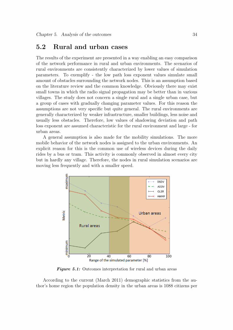
Chapter 5. Analysis of the outcomes 34
5.2 Rural and urban cases
The results of the experiment are presented in a way enabling an easy comparisonof the network performance in rural and urban environments. The scenarios ofrural environments are consistently characterized by lower values of simulationparameters. To exemplify - the low path loss exponent values simulate smallamount of obstacles surrounding the network nodes. This is an assumption basedon the literature review and the common knowledge. Obviously there may existsmall towns in which the radio signal propagation may be better than in variousvillages. The study does not concern a single rural and a single urban case, buta group of cases with gradually changing parameter values. For this reason theassumptions are not very specific but quite general. The rural environments aregenerally characterized by weaker infrastructure, smaller buildings, less noise andusually less obstacles. Therefore, low values of shadowing deviation and pathloss exponent are assumed characteristic for the rural environment and large - forurban areas.
A general assumption is also made for the mobility simulations. The moremobile behavior of the network nodes is assigned to the urban environments. Anexplicit reason for this is the common use of wireless devices during the dailyrides by a bus or tram. This activity is commonly observed in almost every citybut in hardly any village. Therefore, the nodes in rural simulation scenarios aremoving less frequently and with a smaller speed.
Figure 5.1: Outcomes interpretation for rural and urban areas
According to the current (March 2011) demographic statistics from the au-thor’s home region the population density in the urban areas is 1088 citizens per

Chapter 5. Analysis of the outcomes 35
square km. In the rural areas it is equal to 51 people per square km. This is a fact,based on which the density in the rural network scenarios may be assumed to belower than for urban scenarios. Analogically the size of a city is usually smallerthan the size of a village, and even more - than the inhabited part of a villagearea. This is why in the scalability simulations, the rural areas are representedby smaller topologies, and urban - by larger.
The diagram visible in figure 5.1 presents schematically the proposed way ofdisplaying and interpreting the outcomes of the experiment. The lower range ofparameter values, marked by a green rectangle, represents the rural environments.The higher range, in a pale red rectangle, represents the urban environments. Asmentioned before no exact single character of a rural or urban case is defined.Hence an exact limit for the parameter range cannot be set. Since no cleardemarcation between the types of areas is placed, the parameter ranges (red andgreen rectangle in the diagram, figure 5.1) overlap each other partially.
The reason for this kind of outcomes representation is the attempt to simplifythe analysis process and make the observations more intuitive. This way thenetwork performance in rural areas is in general observed in the left part of theabscissa axis. The right part of the abscissa axis refers to the urban WMNscenarios.
5.3 Experiments for UDP traffic
The User Datagram Protocol (UDP) along with the Transmission Control Proto-col (TCP) are the most popular transport protocols. Because of its character, theUDP is also called the Unreliable Datagram Protocol. There are no mechanismsof confirming the delivery of a datagram; therefore, no UDP does not use retrans-mission procedures and does not give any control of the transmitted datagrams.As a result, loss, duplication or confusion of the order of the sent datagrams mayoccur. No connection between transmission source and destination is created, thedata is sent without any settlement with the receiver. Sender has no informationwhether the datagram was received correctly so in case of errors, the retransmis-sion is not possible. The unreliability of UDP is balanced by high transmissionspeed and efficiency. These are the main advantages of UDP making it perfect forthe applications requiring high transmission speed but not vulnerable to partialdata loss e.g. video conferences or media streaming (IPTV, VOIP).
5.3.1 Impact of shadowing deviation
The results of this experiment are presented in table A.1 containing averaged out-comes for all metrics as functions of shadowing deviation. Further those resultsare shown in graphical form of diagrams 5.2, 5.3, 5.4 and 5.5.
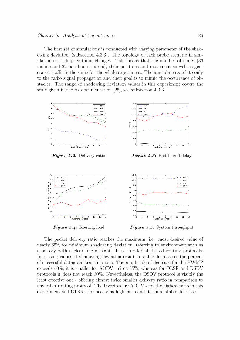
Chapter 5. Analysis of the outcomes 36
The first set of simulations is conducted with varying parameter of the shad-owing deviation (subsection 4.3.3). The topology of each probe scenario in sim-ulation set is kept without changes. This means that the number of nodes (36mobile and 22 backbone routers), their positions and movement as well as gen-erated traffic is the same for the whole experiment. The amendments relate onlyto the radio signal propagation and their goal is to mimic the occurrence of ob-stacles. The range of shadowing deviation values in this experiment covers thescale given in the ns documentation [25], see subsection 4.3.3.
Figure 5.2: Delivery ratio Figure 5.3: End to end delay
Figure 5.4: Routing load Figure 5.5: System throughput
The packet delivery ratio reaches the maximum, i.e. most desired value ofnearly 65% for minimum shadowing deviation, referring to environment such asa factory with a clear line of sight. It is true for all tested routing protocols.Increasing values of shadowing deviation result in stable decrease of the percentof successful datagram transmissions. The amplitude of decrease for the HWMPexceeds 40%; it is smaller for AODV - circa 35%, whereas for OLSR and DSDVprotocols it does not reach 30%. Nevertheless, the DSDV protocol is visibly theleast effective one - offering almost twice smaller delivery ratio in comparison toany other routing protocol. The favorites are AODV - for the highest ratio in thisexperiment and OLSR - for nearly as high ratio and its more stable decrease.
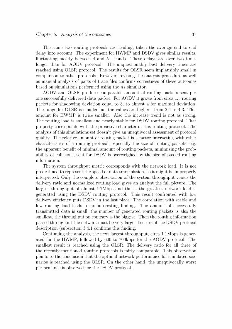
Chapter 5. Analysis of the outcomes 37
The same two routing protocols are leading, taken the average end to enddelay into account. The experiment for HWMP and DSDV gives similar results,fluctuating mostly between 4 and 5 seconds. These delays are over two timeslonger than for AODV protocol. The unquestionably best delivery times arereached using OLSR protocol. The results for OLSR seem implausibly small incomparison to other protocols. However, revising the analysis procedure as wellas manual analysis of parts of trace files confirms correctness of these outcomesbased on simulations performed using the ns simulator.
AODV and OLSR produce comparable amount of routing packets sent perone successfully delivered data packet. For AODV it grows from circa 1.5 routingpackets for shadowing deviation equal to 3, to almost 4 for maximal deviation.The range for OLSR is smaller but the values are higher - from 2.4 to 4.3. Thisamount for HWMP is twice smaller. Also the increase trend is not as strong.The routing load is smallest and nearly stable for DSDV routing protocol. Thatproperty corresponds with the proactive character of this routing protocol. Theanalysis of this simulations set doesn’t give an unequivocal assessment of protocolquality. The relative amount of routing packet is a factor interacting with othercharacteristics of a routing protocol, especially the size of routing packets, e.g.the apparent benefit of minimal amount of routing packets, minimizing the prob-ability of collisions, sent for DSDV is overweighed by the size of passed routinginformation.
The system throughput metric corresponds with the network load. It is notpredestined to represent the speed of data transmission, as it might be improperlyinterpreted. Only the complete observation of the system throughput versus thedelivery ratio and normalized routing load gives an analyst the full picture. Thelargest throughput of almost 1.7Mbps and thus - the greatest network load isgenerated using the DSDV routing protocol. This result confronted with lowdelivery efficiency puts DSDV in the last place. The correlation with stable andlow routing load leads to an interesting finding. The amount of successfullytransmitted data is small, the number of generated routing packets is also thesmallest, the throughput on contrary is the biggest. Then the routing informationpassed throughout the network must be very large. Lecture of the DSDV protocoldescription (subsection 3.4.1 confirms this finding.
Continuing the analysis, the next largest throughput, circa 1.1Mbps is gener-ated for the HWMP, followed by 600 to 700kbps for the AODV protocol. Thesmallest result is reached using the OLSR. The delivery ratio for all three ofthe recently mentioned routing protocols is fairly comparable. This observationpoints to the conclusion that the optimal network performance for simulated sce-narios is reached using the OLSR. On the other hand, the unequivocally worstperformance is observed for the DSDV protocol.
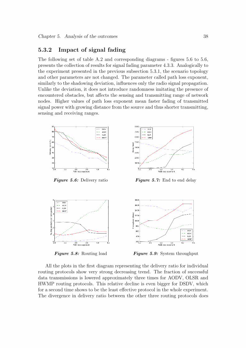
Chapter 5. Analysis of the outcomes 38
5.3.2 Impact of signal fading
The following set of table A.2 and corresponding diagrams - figures 5.6 to 5.6,presents the collection of results for signal fading parameter 4.3.3. Analogically tothe experiment presented in the previous subsection 5.3.1, the scenario topologyand other parameters are not changed. The parameter called path loss exponent,similarly to the shadowing deviation, influences only the radio signal propagation.Unlike the deviation, it does not introduce randomness imitating the presence ofencountered obstacles, but affects the sensing and transmitting range of networknodes. Higher values of path loss exponent mean faster fading of transmittedsignal power with growing distance from the source and thus shorter transmitting,sensing and receiving ranges.
Figure 5.6: Delivery ratio Figure 5.7: End to end delay
Figure 5.8: Routing load Figure 5.9: System throughput
All the plots in the first diagram representing the delivery ratio for individualrouting protocols show very strong decreasing trend. The fraction of successfuldata transmissions is lowered approximately three times for AODV, OLSR andHWMP routing protocols. This relative decline is even bigger for DSDV, whichfor a second time shows to be the least effective protocol in the whole experiment.The divergence in delivery ratio between the other three routing protocols does
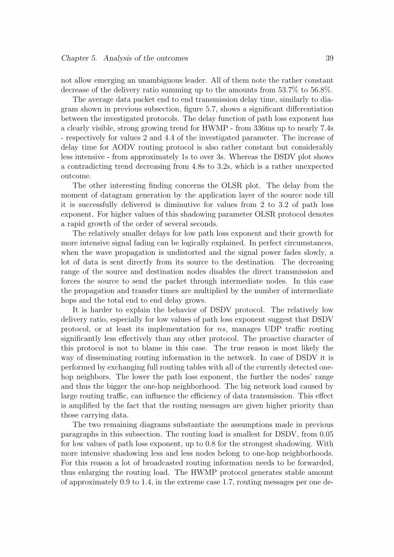
Chapter 5. Analysis of the outcomes 39
not allow emerging an unambiguous leader. All of them note the rather constantdecrease of the delivery ratio summing up to the amounts from 53.7% to 56.8%.
The average data packet end to end transmission delay time, similarly to dia-gram shown in previous subsection, figure 5.7, shows a significant differentiationbetween the investigated protocols. The delay function of path loss exponent hasa clearly visible, strong growing trend for HWMP - from 336ms up to nearly 7.4s- respectively for values 2 and 4.4 of the investigated parameter. The increase ofdelay time for AODV routing protocol is also rather constant but considerablyless intensive - from approximately 1s to over 3s. Whereas the DSDV plot showsa contradicting trend decreasing from 4.8s to 3.2s, which is a rather unexpectedoutcome.
The other interesting finding concerns the OLSR plot. The delay from themoment of datagram generation by the application layer of the source node tillit is successfully delivered is diminutive for values from 2 to 3.2 of path lossexponent. For higher values of this shadowing parameter OLSR protocol denotesa rapid growth of the order of several seconds.
The relatively smaller delays for low path loss exponent and their growth formore intensive signal fading can be logically explained. In perfect circumstances,when the wave propagation is undistorted and the signal power fades slowly, alot of data is sent directly from its source to the destination. The decreasingrange of the source and destination nodes disables the direct transmission andforces the source to send the packet through intermediate nodes. In this casethe propagation and transfer times are multiplied by the number of intermediatehops and the total end to end delay grows.
It is harder to explain the behavior of DSDV protocol. The relatively lowdelivery ratio, especially for low values of path loss exponent suggest that DSDVprotocol, or at least its implementation for ns, manages UDP traffic routingsignificantly less effectively than any other protocol. The proactive character ofthis protocol is not to blame in this case. The true reason is most likely theway of disseminating routing information in the network. In case of DSDV it isperformed by exchanging full routing tables with all of the currently detected one-hop neighbors. The lower the path loss exponent, the further the nodes’ rangeand thus the bigger the one-hop neighborhood. The big network load caused bylarge routing traffic, can influence the efficiency of data transmission. This effectis amplified by the fact that the routing messages are given higher priority thanthose carrying data.
The two remaining diagrams substantiate the assumptions made in previousparagraphs in this subsection. The routing load is smallest for DSDV, from 0.05for low values of path loss exponent, up to 0.8 for the strongest shadowing. Withmore intensive shadowing less and less nodes belong to one-hop neighborhoods.For this reason a lot of broadcasted routing information needs to be forwarded,thus enlarging the routing load. The HWMP protocol generates stable amountof approximately 0.9 to 1.4, in the extreme case 1.7, routing messages per one de-
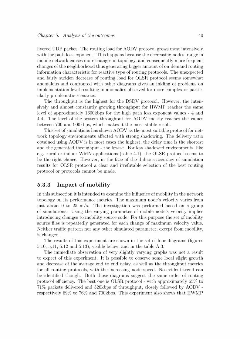
Chapter 5. Analysis of the outcomes 40
livered UDP packet. The routing load for AODV protocol grows most intensivelywith the path loss exponent. This happens because the decreasing nodes’ range inmobile network causes more changes in topology, and consequently more frequentchanges of the neighborhood thus generating bigger amount of on-demand routinginformation characteristic for reactive type of routing protocols. The unexpectedand fairly sudden decrease of routing load for OLSR protocol seems somewhatanomalous and confronted with other diagrams gives an inkling of problems onimplementation level resulting in anomalies observed for more complex or partic-ularly problematic scenarios.
The throughput is the highest for the DSDV protocol. However, the inten-sively and almost constantly growing throughput for HWMP reaches the samelevel of approximately 1600kbps for the high path loss exponent values - 4 and4.4. The level of the system throughput for AODV mostly reaches the valuesbetween 700 and 900kbps, which makes it the most stable result.
This set of simulations has shown AODV as the most suitable protocol for net-work topology environments affected with strong shadowing. The delivery ratioobtained using AODV is in most cases the highest, the delay time is the shortestand the generated throughput - the lowest. For less shadowed environments, likee.g. rural or indoor WMN applications (table 4.1), the OLSR protocol seems tobe the right choice. However, in the face of the dubious accuracy of simulationresults for OLSR protocol a clear and irrefutable selection of the best routingprotocol or protocols cannot be made.
5.3.3 Impact of mobility
In this subsection it is intended to examine the influence of mobility in the networktopology on its performance metrics. The maximum node’s velocity varies fromjust about 0 to 25 m/s. The investigation was performed based on a groupof simulations. Using the varying parameter of mobile node’s velocity impliesintroducing changes to mobility source code. For this purpose the set of mobilitysource files is repeatedly generated for each change of maximum velocity value.Neither traffic pattern nor any other simulated parameter, except from mobility,is changed.
The results of this experiment are shown in the set of four diagrams (figures5.10, 5.11, 5.12 and 5.13), visible below, and in the table A.3.
The immediate observation of very slightly varying graphs was not a resultto expect of this experiment. It is possible to observe some local slight growthand decrease of the average end to end delay, as well as the throughput metricsfor all routing protocols, with the increasing node speed. No evident trend canbe identified though. Both those diagrams suggest the same order of routingprotocol efficiency. The best one is OLSR protocol - with approximately 65% to71% packets delivered and 320kbps of throughput, closely followed by AODV -respectively 69% to 76% and 700kbps. This experiment also shows that HWMP
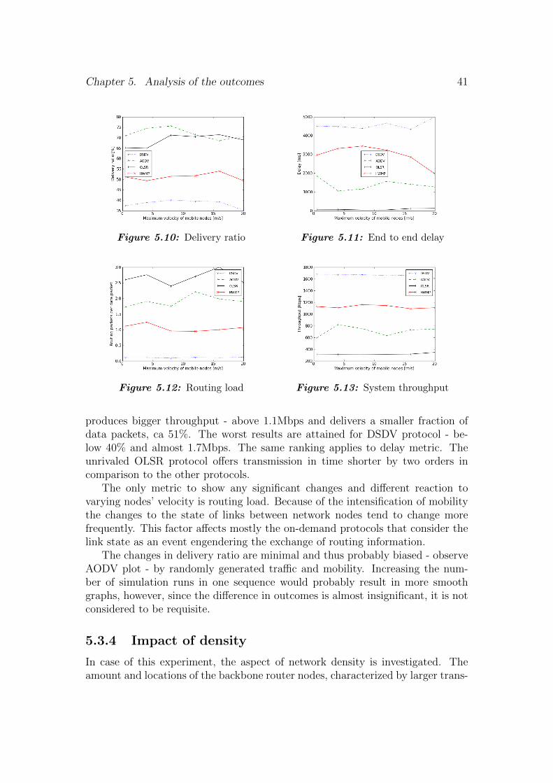
Chapter 5. Analysis of the outcomes 41
Figure 5.10: Delivery ratio Figure 5.11: End to end delay
Figure 5.12: Routing load Figure 5.13: System throughput
produces bigger throughput - above 1.1Mbps and delivers a smaller fraction ofdata packets, ca 51%. The worst results are attained for DSDV protocol - be-low 40% and almost 1.7Mbps. The same ranking applies to delay metric. Theunrivaled OLSR protocol offers transmission in time shorter by two orders incomparison to the other protocols.
The only metric to show any significant changes and different reaction tovarying nodes’ velocity is routing load. Because of the intensification of mobilitythe changes to the state of links between network nodes tend to change morefrequently. This factor affects mostly the on-demand protocols that consider thelink state as an event engendering the exchange of routing information.
The changes in delivery ratio are minimal and thus probably biased - observeAODV plot - by randomly generated traffic and mobility. Increasing the num-ber of simulation runs in one sequence would probably result in more smoothgraphs, however, since the difference in outcomes is almost insignificant, it is notconsidered to be requisite.
5.3.4 Impact of density
In case of this experiment, the aspect of network density is investigated. Theamount and locations of the backbone router nodes, characterized by larger trans-

Chapter 5. Analysis of the outcomes 42
mission power and lower sensing and receiving threshold, another words - largerrange, remains unchanged. The alterations are applied only to the number of themobile nodes, which also implies changes to their mobility generated randomlyusing setdest movement generator. The density of nodes is characterized by thenumber of the mobile nodes per one backbone router. The density varies in rangefrom 0.5 to 3.5. The results are shown in the table A.4 and diagrams: 5.14, 5.15,5.16 and 5.17.
Figure 5.14: Delivery ratio Figure 5.15: End to end delay
The outcomes once again give the leadership to the OLSR and AODV routingprotocols and puts DSDV in the last place. The delivery ratio is almost the same- starting at ca 73% and gradually decreasing for both OLSR and AODV. TheOLSR protocol leads in case of the packet delay, mostly in hundredths of a secondrow, and the throughput metric - decreasing from 558 to 211kbps, but AODVoutranks it in case of routing load. The OLSR plots for delivery ratio and routingload metrics show a sudden drop for the highest nodes’ density. This suspiciousbehavior was already denoted before in subsection 5.3.2 for high values of pathloss exponent; therefore, those outcomes seem to confirm the previous assumptionof anomalies in complex scenarios using OLSR protocol.
The growth of mobile nodes density has a significant influence on the deliveryratio causing the decrease of 19 - 43% for the extreme values of the parameter.The largest fall of packet delivery fraction, apart from the sudden drop for OLSR,refers to the DSDV protocol.
The average packet delay time for DSDV and HWMP decreases intensivelytogether with the delivery ratio. Its amplitude for the extreme low and highdensity is over 2.5s for the HWMP and almost 3.8s for the DSDV protocol. Forthe OLSR protocol the end to end delay time seems to be rather constant exceptfrom the initial drop from 511ms through 146ms to 52ms. The AODV on contrarydenotes slight growth from ca 2s to 2.5s.
The more mobile nodes the higher the routing load. This correlation is com-mon for all the investigated protocols. The only local and very large decrease forOLSR protocol is considered a result of a fault in the simulation tool or proto-col implementation. The growth is intensive for protocols reacting to changes in
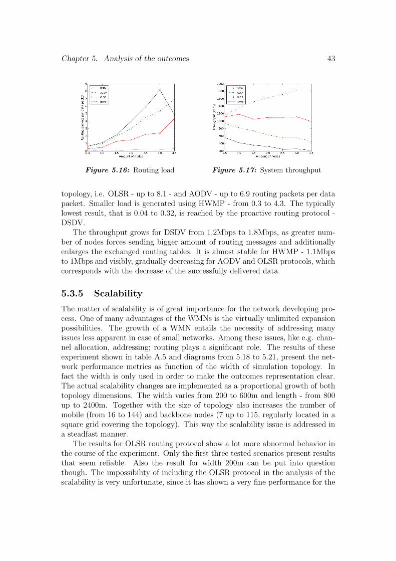
Chapter 5. Analysis of the outcomes 43
Figure 5.16: Routing load Figure 5.17: System throughput
topology, i.e. OLSR - up to 8.1 - and AODV - up to 6.9 routing packets per datapacket. Smaller load is generated using HWMP - from 0.3 to 4.3. The typicallylowest result, that is 0.04 to 0.32, is reached by the proactive routing protocol -DSDV.
The throughput grows for DSDV from 1.2Mbps to 1.8Mbps, as greater num-ber of nodes forces sending bigger amount of routing messages and additionallyenlarges the exchanged routing tables. It is almost stable for HWMP - 1.1Mbpsto 1Mbps and visibly, gradually decreasing for AODV and OLSR protocols, whichcorresponds with the decrease of the successfully delivered data.
5.3.5 Scalability
The matter of scalability is of great importance for the network developing pro-cess. One of many advantages of the WMNs is the virtually unlimited expansionpossibilities. The growth of a WMN entails the necessity of addressing manyissues less apparent in case of small networks. Among these issues, like e.g. chan-nel allocation, addressing; routing plays a significant role. The results of theseexperiment shown in table A.5 and diagrams from 5.18 to 5.21, present the net-work performance metrics as function of the width of simulation topology. Infact the width is only used in order to make the outcomes representation clear.The actual scalability changes are implemented as a proportional growth of bothtopology dimensions. The width varies from 200 to 600m and length - from 800up to 2400m. Together with the size of topology also increases the number ofmobile (from 16 to 144) and backbone nodes (7 up to 115, regularly located in asquare grid covering the topology). This way the scalability issue is addressed ina steadfast manner.
The results for OLSR routing protocol show a lot more abnormal behavior inthe course of the experiment. Only the first three tested scenarios present resultsthat seem reliable. Also the result for width 200m can be put into questionthough. The impossibility of including the OLSR protocol in the analysis of thescalability is very unfortunate, since it has shown a very fine performance for the
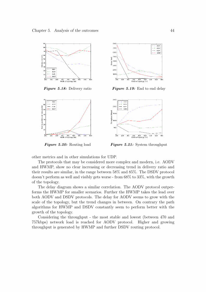
Chapter 5. Analysis of the outcomes 44
Figure 5.18: Delivery ratio Figure 5.19: End to end delay
Figure 5.20: Routing load Figure 5.21: System throughput
other metrics and in other simulations for UDP.The protocols that may be considered more complex and modern, i.e. AODV
and HWMP, show no clear increasing or decreasing trend in delivery ratio andtheir results are similar, in the range between 58% and 85%. The DSDV protocoldoesn’t perform as well and visibly gets worse - from 68% to 33%, with the growthof the topology.
The delay diagram shows a similar correlation. The AODV protocol outper-forms the HWMP for smaller scenarios. Further the HWMP takes the lead overboth AODV and DSDV protocols. The delay for AODV seems to grow with thescale of the topology, but the trend changes in between. On contrary the pathalgorithms for HWMP and DSDV constantly seem to perform better with thegrowth of the topology.
Considering the throughput - the most stable and lowest (between 470 and757kbps) network load is reached for AODV protocol. Higher and growingthroughput is generated by HWMP and further DSDV routing protocol.
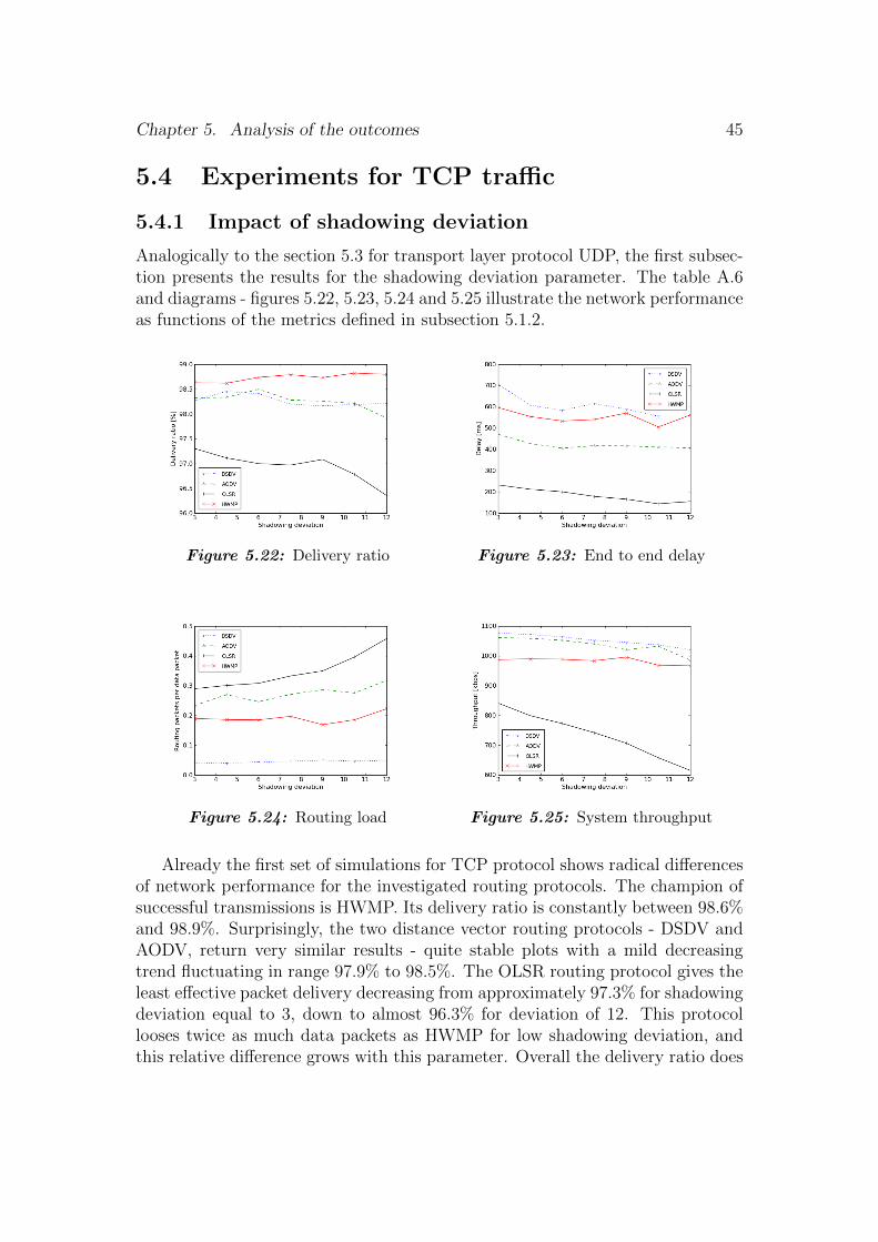
Chapter 5. Analysis of the outcomes 45
5.4 Experiments for TCP traffic
5.4.1 Impact of shadowing deviation
Analogically to the section 5.3 for transport layer protocol UDP, the first subsec-tion presents the results for the shadowing deviation parameter. The table A.6and diagrams - figures 5.22, 5.23, 5.24 and 5.25 illustrate the network performanceas functions of the metrics defined in subsection 5.1.2.
Figure 5.22: Delivery ratio Figure 5.23: End to end delay
Figure 5.24: Routing load Figure 5.25: System throughput
Already the first set of simulations for TCP protocol shows radical differencesof network performance for the investigated routing protocols. The champion ofsuccessful transmissions is HWMP. Its delivery ratio is constantly between 98.6%and 98.9%. Surprisingly, the two distance vector routing protocols - DSDV andAODV, return very similar results - quite stable plots with a mild decreasingtrend fluctuating in range 97.9% to 98.5%. The OLSR routing protocol gives theleast effective packet delivery decreasing from approximately 97.3% for shadowingdeviation equal to 3, down to almost 96.3% for deviation of 12. This protocollooses twice as much data packets as HWMP for low shadowing deviation, andthis relative difference grows with this parameter. Overall the delivery ratio does
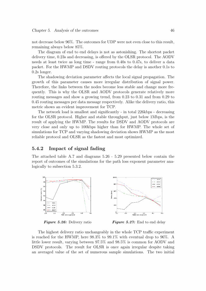
Chapter 5. Analysis of the outcomes 46
not decrease below 96%. The outcomes for UDP were not even close to this result,remaining always below 85%.
The diagram of end to end delays is not as astonishing. The shortest packetdelivery time, 0.23s and decreasing, is offered by the OLSR protocol. The AODVneeds at least twice as long time - range from 0.40s to 0.47s, to deliver a datapacket. For the HWMP and DSDV routing protocols the delay is another 0.1s to0.2s longer.
The shadowing deviation parameter affects the local signal propagation. Thegrowth of this parameter causes more irregular distribution of signal power.Therefore, the links between the nodes become less stable and change more fre-quently. This is why the OLSR and AODV protocols generate relatively morerouting messages and show a growing trend, from 0.23 to 0.31 and from 0.29 to0.45 routing messages per data message respectively. Alike the delivery ratio, thismetric shows an evident improvement for TCP.
The network load is smallest and significantly - in total 226kbps - decreasingfor the OLSR protocol. Higher and stable throughput, just below 1Mbps, is theresult of applying the HWMP. The results for DSDV and AODV protocols arevery close and only up to 100kbps higher than for HWMP. The whole set ofsimulations for TCP and varying shadowing deviation shows HWMP as the mostreliable protocol and OLSR as the fastest and most optimized.
5.4.2 Impact of signal fading
The attached table A.7 and diagrams 5.26 - 5.29 presented below contain thereport of outcomes of the simulations for the path loss exponent parameter ana-logically to subsection 5.3.2.
Figure 5.26: Delivery ratio Figure 5.27: End to end delay
The highest delivery ratio unchangeably in the whole TCP traffic experimentis reached for the HWMP, here 98.3% to 99.1% with eventual drop to 96%. Alittle lower result, varying between 97.5% and 98.5% is common for AODV andDSDV protocols. The result for OLSR is once again irregular despite takingan averaged value of the set of numerous sample simulations. The two initial
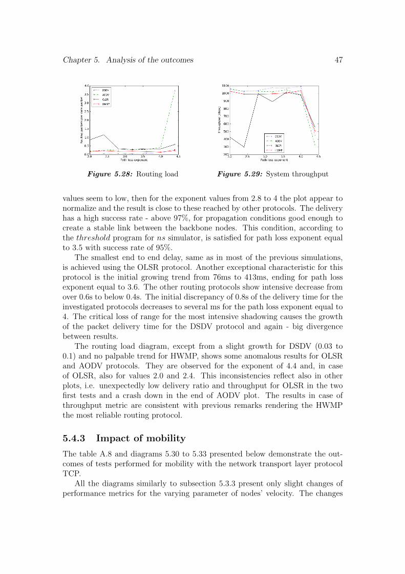
Chapter 5. Analysis of the outcomes 47
Figure 5.28: Routing load Figure 5.29: System throughput
values seem to low, then for the exponent values from 2.8 to 4 the plot appear tonormalize and the result is close to these reached by other protocols. The deliveryhas a high success rate - above 97%, for propagation conditions good enough tocreate a stable link between the backbone nodes. This condition, according tothe threshold program for ns simulator, is satisfied for path loss exponent equalto 3.5 with success rate of 95%.
The smallest end to end delay, same as in most of the previous simulations,is achieved using the OLSR protocol. Another exceptional characteristic for thisprotocol is the initial growing trend from 76ms to 413ms, ending for path lossexponent equal to 3.6. The other routing protocols show intensive decrease fromover 0.6s to below 0.4s. The initial discrepancy of 0.8s of the delivery time for theinvestigated protocols decreases to several ms for the path loss exponent equal to4. The critical loss of range for the most intensive shadowing causes the growthof the packet delivery time for the DSDV protocol and again - big divergencebetween results.
The routing load diagram, except from a slight growth for DSDV (0.03 to0.1) and no palpable trend for HWMP, shows some anomalous results for OLSRand AODV protocols. They are observed for the exponent of 4.4 and, in caseof OLSR, also for values 2.0 and 2.4. This inconsistencies reflect also in otherplots, i.e. unexpectedly low delivery ratio and throughput for OLSR in the twofirst tests and a crash down in the end of AODV plot. The results in case ofthroughput metric are consistent with previous remarks rendering the HWMPthe most reliable routing protocol.
5.4.3 Impact of mobility
The table A.8 and diagrams 5.30 to 5.33 presented below demonstrate the out-comes of tests performed for mobility with the network transport layer protocolTCP.
All the diagrams similarly to subsection 5.3.3 present only slight changes ofperformance metrics for the varying parameter of nodes’ velocity. The changes
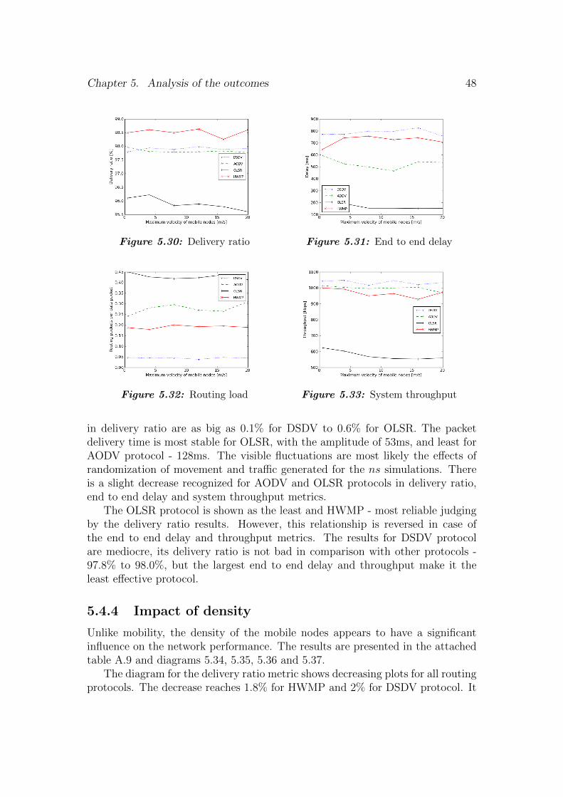
Chapter 5. Analysis of the outcomes 48
Figure 5.30: Delivery ratio Figure 5.31: End to end delay
Figure 5.32: Routing load Figure 5.33: System throughput
in delivery ratio are as big as 0.1% for DSDV to 0.6% for OLSR. The packetdelivery time is most stable for OLSR, with the amplitude of 53ms, and least forAODV protocol - 128ms. The visible fluctuations are most likely the effects ofrandomization of movement and traffic generated for the ns simulations. Thereis a slight decrease recognized for AODV and OLSR protocols in delivery ratio,end to end delay and system throughput metrics.
The OLSR protocol is shown as the least and HWMP - most reliable judgingby the delivery ratio results. However, this relationship is reversed in case ofthe end to end delay and throughput metrics. The results for DSDV protocolare mediocre, its delivery ratio is not bad in comparison with other protocols -97.8% to 98.0%, but the largest end to end delay and throughput make it theleast effective protocol.
5.4.4 Impact of density
Unlike mobility, the density of the mobile nodes appears to have a significantinfluence on the network performance. The results are presented in the attachedtable A.9 and diagrams 5.34, 5.35, 5.36 and 5.37.
The diagram for the delivery ratio metric shows decreasing plots for all routingprotocols. The decrease reaches 1.8% for HWMP and 2% for DSDV protocol. It
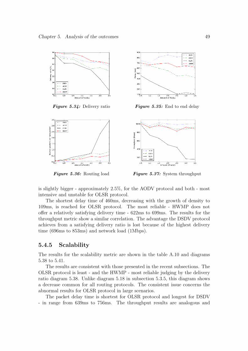
Chapter 5. Analysis of the outcomes 49
Figure 5.34: Delivery ratio Figure 5.35: End to end delay
Figure 5.36: Routing load Figure 5.37: System throughput
is slightly bigger - approximately 2.5%, for the AODV protocol and both - mostintensive and unstable for OLSR protocol.
The shortest delay time of 460ms, decreasing with the growth of density to109ms, is reached for OLSR protocol. The most reliable - HWMP does notoffer a relatively satisfying delivery time - 622ms to 699ms. The results for thethroughput metric show a similar correlation. The advantage the DSDV protocolachieves from a satisfying delivery ratio is lost because of the highest deliverytime (696ms to 853ms) and network load (1Mbps).
5.4.5 Scalability
The results for the scalability metric are shown in the table A.10 and diagrams5.38 to 5.41.
The results are consistent with those presented in the recent subsections. TheOLSR protocol is least - and the HWMP - most reliable judging by the deliveryratio diagram 5.38. Unlike diagram 5.18 in subsection 5.3.5, this diagram showsa decrease common for all routing protocols. The consistent issue concerns theabnormal results for OLSR protocol in large scenarios.
The packet delay time is shortest for OLSR protocol and longest for DSDV- in range from 639ms to 756ms. The throughput results are analogous and
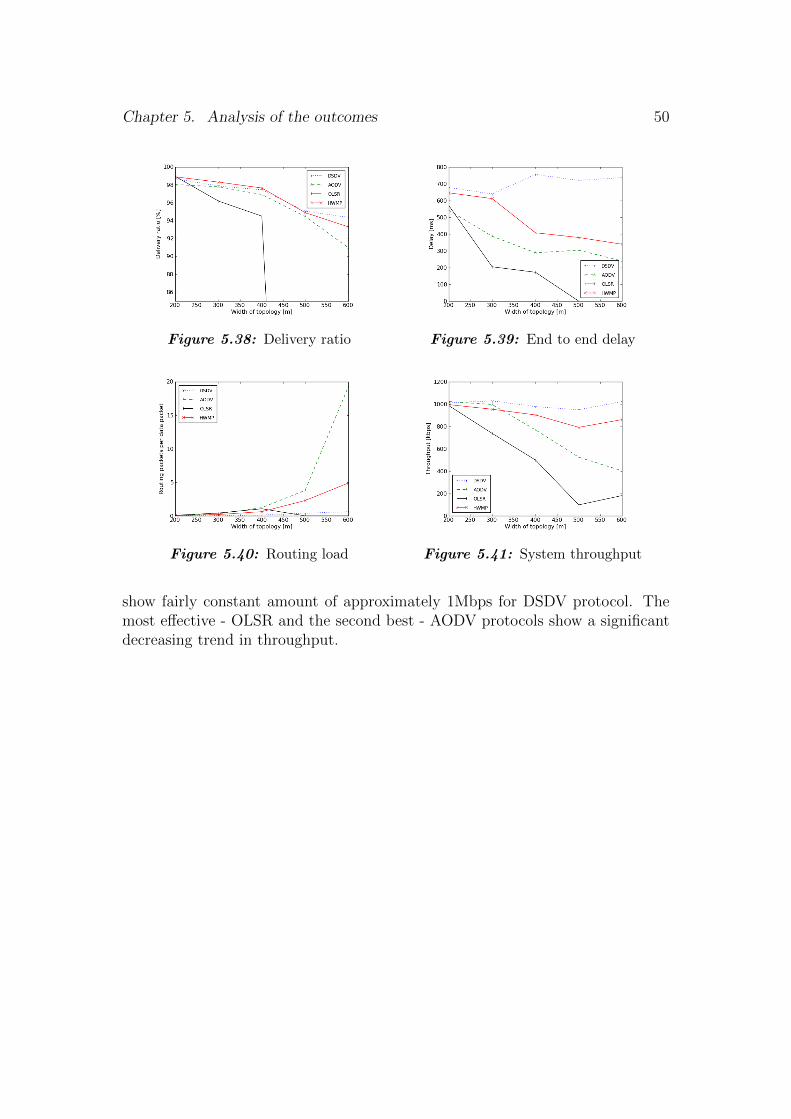
Chapter 5. Analysis of the outcomes 50
Figure 5.38: Delivery ratio Figure 5.39: End to end delay
Figure 5.40: Routing load Figure 5.41: System throughput
show fairly constant amount of approximately 1Mbps for DSDV protocol. Themost effective - OLSR and the second best - AODV protocols show a significantdecreasing trend in throughput.
Chapter 6
Discussion
6.1 Interpretation and summary of the outcomes
The obtained results, analyzed systematically in logically ordered groups for TCPand UDP transport protocols, give an overview of the influence of diverse exter-nal factors on the network performance. As explained in chapter 5 the TORAalgorithm was excluded from the analysis. The content of this chapter is an over-all discussion of the results and the final assessment. The experiment is beingviewed from three different perspectives corresponding with the type of simulatedfactors influencing the network performance. At first the propagation issues areconsidered, then the nodes mobility results are shortly concluded, to finish withthe summary of the network density and size issue.
The first two sets of simulations, both for UDP and TCP, are investigatingthe impact of the propagation factors such as physical obstacles weakening anddistorting the signal. The event of encountering an obstacle by the radio wavesresults in two kinds of phenomena, which affect the wave - reflection and attenua-tion. The aggregate effect of an obstacle in consequence weakens the signal powerand changes its distribution around the source. The experiment has shown visibledifferences between the network performance in the varying propagation condi-tions in rural and urban residential areas. They are especially evident in case ofsimulations with the UDP traffic, where the delivery ratio is significantly betterfor rural than urban areas. With the growth of both of the shadowing parameters(shadowing deviation and path loss exponent, representing the distortion of theradio signal caused by the presence of obstacles) the delivery ratio of the UDPdata packets significantly decreases. In case of the TCP connections the corre-lation is not that evident. On contrary, the delivery ratio is almost the same oreven slightly better for urban environment. The delivery decreases rapidly onlyin the simulations with the most extreme value of path loss exponent parameter(4.4), which symbolizes a very intensively shadowed urban area.
The end to end delay results, when crosschecked, show an astonishing finding.Namely, the delay time for the TCP is, in most of the cases, several times shorterthan for UDP. The relation is expected to be reverse. The UDP’s weakness is thelack of control and a high probability of loosing data packets. This characteristic
51
Chapter 6. Discussion 52
is well pictured by the delivery ratio diagrams showing values for the UDP reducedby several tens percent in comparison to TCP’s ratio. That is the price paid fora quicker and more agile transmission. Meanwhile, the delivery time for TCPis not only much lower than for UDP, but moreover, it is still decreasing withthe deteriorating conditions of propagation. According to a large part of theexperiment outcomes for the TCP traffic the intensively shadowed urban areasare more beneficial for network performance than obstacle-free rural areas.
The only results consistent with the logical predictions can be observed forthe OLSR protocol. Intensification of the propagation shadowing in case of theOLSR protocol results in lower network performance, which may be observedfor all demonstrated metrics. The delivery ratio decreases with the increase ofshadowing deviation and path loss exponent, with an exception for the path lossexponent diagram for TCP, which shows an increase and some anomalous resultsfor the extreme parameter values. Nevertheless, this suspicious behavior can berationally explained. The blame for the anomalous results for exponent 2.0 and2.4 is to be put on the simulation tool. The delivery ratio is kept so high thanksto controlling the transport and, if necessary, retransmitting the lost packets untiltheir successful delivery is acknowledged. As long as it is possible to find any paththrough the network connecting the transmission source with the destination, thepacket can be delivered. When the propagation deteriorates, less and less pathsin the network are available. The obvious consequence is the increase of the pathfinding time and larger number of retransmissions as more transmission errorsoccur. To sum up, the average end to end delay of a data packet transmissionis expected to increase when the propagation weakens. An observation of theOLSR plots in the diagrams analyzed in subsection 5.4.2 corresponds well withthese theoretical contemplations. As long as the weakening propagation condi-tions (path loss exponent 2.8 to 4.0) allow finding a path connecting the sourcewith the destination, the delivery ratio is kept high at the cost of a lengthenedtransmission time. An incomplete network graph, as for exponent 4.4 causes moredelivery failures and since the path may not be found, no more retransmissionstake place. This is why both - delivery ratio and delivery time, decrease in theworst propagation conditions.
Judging the quality of the routing protocols based on the simulation results,the HWMP protocol provides the best delivery ratio for TCP traffic and a goodratio for UDP traffic in most of the investigated cases of both - rural and urbanpropagation conditions. However, the results for the delivery time metric, onlycomparable with DSDV, are rather unsatisfactory. Unquestionably best deliverytime, i.e. shortest end to end delay is provided by the OLSR protocol. The largestcontrast is visible for the low values of the path loss exponent representing therural environment. Also the network load for the OLSR is the most optimal. TheDSDV protocol with its large network load and long end to end delay is recom-mended neither for the rural nor urban environment. The results for the AODVprotocol can be described as more balanced, as the AODV plots usually oscillate
Chapter 6. Discussion 53
between the HWMP and OLSR plots, which can be also considered an advantage.Taken all the metrics in consideration the OLSR is the most optimal of the in-vestigated protocols, however, it is not unsurpassed in all of the investigated cases.
The outcomes for mobility, for both - the TCP and the UDP, show no significantimpact of nodes’ movement velocity and intensity on the network performance.Therefore, for all simulated cases of rural and urban environments the results andrecommendations are similar. The overall results point out the OLSR protocolas the most optimal, with the exception in case of the delivery ratio for the TCPtraffic. In this case the successful delivery rate of the OLSR protocol is from 1.5%to 3% worse than of the other protocols.
Unlike the mobility, the impact of the density of network nodes and the size of thetopology on the network performance is clearly visible. The scale of this influenceis more or less comparable with the propagation parameters. What makes thesetwo groups of simulations differ from the others is a clearly visible decrease ofthe delivery ratio also for the TCP traffic. From this overall observation we mayconclude that the size and density of network topology have a direct influenceon the rate of successful deliveries of the data packets. As expected, the deliveryratio for the TCP traffic is higher and decreases slower with increasing number ofnodes than for UDP traffic. Nevertheless, a clear and constant decreasing trendfor the TCP is observed. Taken this metric into consideration, the leading pro-tocols are HWMP and AODV. The DSDV protocol plots show weak results forthe UDP traffic. On the other hand the OLSR protocol performs worse for theTCP traffic and unfortunately a large part of the simulation results with increas-ing complexity of the topology is invalid. However, the valid part of outcomes,mostly covering the settings representing the rural network applications, demon-strates yet another time the unmatched packet transmission speed obtained forthe OLSR protocol. The second best end to end delay results are generated inthe simulations with applied AODV protocol. Based on the experimentally ob-tained data, the OLSR protocol performs well in the rural environment with adecent delivery ratio and the supreme transmission time. As it is not sensibleto draw conclusions about OLSR performance for urban areas (dense and largetopologies) from the simulations outcomes, only the three remaining protocolsare considered. In this case the choice is a tradeoff between a slightly higherdelivery ratio achieved for the HWMP and a little shorter end to end delay timecharacterizing the outcomes for the AODV protocol.
The ultimate evaluation is not conclusively pointing out one supreme solutionfor routing in all investigated rural and urban application cases of WMNs. Thesimulations for OLSR protocol have shown undeniable advantage of this protocolover any other in case of the packet delivery time metric. However, the deliveryratio for this protocol is not always as good. In case of the experiments with

Chapter 6. Discussion 54
the UDP traffic, the result was the best or at least among the best (the AODVprotocol simulations have shown similar results in delivery ratio). Unfortunatelythe leverage is so apparent only for the UDP. The experiment for the TCP showsthe OLSR protocol as least reliable, what can be observed in almost all deliv-ery ratio diagrams for TCP traffic. Moreover some of the simulations for OLSR,especially for the simulation settings characterizing the urban environment, re-turn results that cannot be considered as credible. In case of TCP traffic theHWMP protocol has shown some highly desirable characteristics. The deliveryratio of the HWMP is the most stable and unmatched by any other protocol inall investigated cases. The leverage becomes more apparent for larger or more in-tensively shadowed topologies which are meant to illustrate the urban conditions.Still the rather mean performance, especially in case of the end to end deliverydelay time in rural conditions, as well as generating a large network load, is thesignificant weaknesses of the HWMP protocol. Moreover a deeper revision of theHWMP implementation may put the outstanding success rate in packets deliveryinto question. There are many calculations that use sometimes subtle, at othertimes quite evident, crosscuts and hoaxes. An example may be found in a codecomment in file hwmp rtable.h, line 82 that says:
We suppose now that we have no errors during retransmitting, therate is constant and equals to 1 Mbit/sec. And the shadowing modelis turned OFF
The quoted fragment of the HWMP implementation file implies that the packetretransmission is most probably biased and no additional impact of the shadowingeffect is taken to consideration. This may be a factor lifting the delivery ratioresult for HWMP. However, only a throughout analysis of the code can be a baseto judge the true quality and credibility of the results.
6.2 The issue of the simulation credibility
In addition to the performance report for the investigated routing protocols inchanging environment, the experiment brought several other issues to light. Therather disturbing discoveries were made during the experiment implementationand running the simulations.
The implementation of a life-like wireless network simulation scenario involvesusing several components responsible for diverse elements of a network. In a realnetwork the randomness of network nodes’ movement and signal propagationplays a significant role. The ns simulator uses a randomization based on RNG(Random Number Generator) e.g. for calculations of the radio signal power.However, the movement of nodes as well as traffic is not generated randomly dur-ing the simulation, unless implemented so, but read from external files containing

Chapter 6. Discussion 55
fixed traffic and movement patterns. As described in section 4.3 there are nsmodules designed for generating this kind of files.
The movement generation program setdest is written in C++ language anduses randomly generated values for determining the direction of movement andspeed of the nodes. The speed is random but not larger than a required maximumspeed argument declared by the user. The way the nodes move is always along astraight line from the initial location to the randomly chosen point. This is notthe way the modes move in reality. They tend to change speed and the directionof movement. There is, however, a more serious reservation. When a node reachesits destination it stops for a while before taking the next trip. The duration of thepause in which the nodes rest is determined by another argument and is alwaysconstant. I.e. if the pause is declared as 20s then every node, after reaching thedestination, makes a 20s long break and then starts to move again to a new point.The worst situation is observed at the beginning of the simulation. This is themoment when all nodes are created and begin their first pause and no movementis observed. After the time passes all of them start moving at the same time as ifit was a start of a race. This behavior cannot be observed in reality either. Thecherry on top is the fact of counting the nodes from 1 and not from 0. This wayif the movement pattern for 50 nodes is generated it is implemented for node 1to 50, not for 0 to 49, which while running a simulation results in a ridiculousno such element in array error. Some minor modifications made this tool usableand less problematic, but still definitely far from perfect.
But what is still more disturbing is the traffic generation module cbrgen (de-scribed in the subsection 4.3.1), so commonly used in course of network research.It is written in OTcl language and ran using ns. The user can choose the typeof connection (UDP or TCP), number of nodes, the interval between subsequentUDP packets and limit of the number of the created connections. As the outputthis ns script generates a set of connection between some nodes at a randommoment. While looking at this module as at a black-box nothing seems to bevery wrong. However, several problems appear after inspecting the script code.Firstly, the time in which the connections are created is reduced to 180s (by mod-ulo operation on a random value). That means that the unmodified version ofcbrgen produces the traffic pattern only for simulations lasting exactly 3 minutes[sic], which could be expected since (unlike setdest) cbrgen does not require anargument defining the duration of the simulation. The second problem concernsthe way the nodes are being connected. The connection is set up between nodeschosen by a rather convoluted algorithm. With each iteration, from 0 to thedeclared number of nodes, a random number in range 0 to 100 is generated. Ifthe number is larger than 50, a connection is created between the node appointedby current value of iteration and the next one. Additionally if the number islarger than 75, another connection will be set between the current node and thevalue of iteration plus 2. This means that each of the nodes may be sending dataonly to his next two successors and receiving from his two predecessors. This
Chapter 6. Discussion 56
assumption already limits the maximum number of connections to double theamount of nodes. The further limitation by the mc - maximum number of con-nections argument [25] causes the connection creating algorithm to stop at theexact moment when the desired number of connections is reached. This meansthat the randomness in case of the cbrgen module is seriously disrupted. Theseissues apart, there is much more to be desired from a traffic generating scriptdistributed as a component along a major scientific research tool.
As mentioned in the beginning of the analysis chapter, the implementation ofthe TORA routing protocol is also distributed along ns as well as e.g. DSDV,AODV protocols. However, unlike those two protocols, TORA implementationdoes not work correctly. The trace files for TORA grow dramatically and don’tcontain data prone to sensible analysis. Searching for solution to this problem onemay encounter publications that apparently were using ns simulations conductedfor TORA and numerous patches and modification instructions. Nevertheless,no case of a successful experiment conducted for TORA with the version 2.34 ofns and similar simulation configuration was found. Applying recommended fixes,patching and an overall code revision did not bring a positive result. Rewriting afaulty routing protocol implementation does not belong to this research, moreoverit is a very time consuming task, and therefore, this protocol was excluded fromfurther investigations.
Except from DSDV, AODV and the discouraged TORA protocol the groupchosen for investigations entailed installing two additional protocols. The task ofadding new protocols is thoroughly described in the ns documentation [25]. Evenmore exhaustive description was included in the implementations of OLSR andHWMP protocols distributed with-, or completely in form of patches. Unfortu-nately this solution is still far from perfect. The patches excluded each other byintroducing changes in the simulator files rendering them insusceptible to otherpatching. Incorporating both of the additional routing protocols required manualmodifications of files intended to be automatically patched using the implemen-tation in patch files.
The use of the shadowing in wireless network simulation also required spe-cial attention. Multiple recalculation of the propagation, transmission power andreceiver parameters were necessary. Minor imprecision and lack of in-deep doc-umentation [25] of the usage of the shadowing model necessitated familiarizingwith the signal propagation implementation files. This eventually gave the under-standing of the shadowing model mechanisms and the true idea of implementingsuch a simulation.
Finally some problems were encountered in the process of interpreting theoutcomes. The trace format is unified for all wireless simulations. In this case socalled newtrace format was used. As long as the trace files were all written inthe same format and looked alike, the content of the trace file line describing anevent for a certain packet was different for different routing protocols. In order toensure an earnest, reliable analysis, the trace format for all protocols was revised

Chapter 6. Discussion 57
and based on that the trace files were processed.Based on experiences with the ns network simulator it is possible to draw
conclusions about the network mechanisms and observe the influence of diversefactors. Nevertheless, in the opinion of the author of this research, it is advisableto be cautious with using ns as a tool determining how the network would functionin reality or relying on the simulation results in the process of choosing networkequipment, planning topology and configuration. Especially, in consideration hasto be taken the fact that no warranty for a faultless functioning or results isgiven, which is reminded in the code of all the components and the ns simulatoritself. Hopefully significant improvements are being implemented in the currentlydeveloped version 3 of the ns simulator. Probably significantly better analyticalaccuracy as well as quality control and support is provided by commercial andenterprise software products designed by and for large network companies.
Chapter 7
Conclusion and future work
This thesis contains the complete documentation of the contributed research workincluding a literature based theoretical introduction, experiment planning, tools,implementation and running, and the subsequent analysis of results. The out-comes are summarized in a discussion chapter which also raises the question ofthe credibility of the simulation tool.
According to the experiment outcomes the performance of WMNs varies stronglyin diverse environments. Topologies characterized as rural show in general betterresults in terms of reliability, time efficiency and network load than the urbanscenarios. The simulated propagation conditions influenced the performance in-tensively, especially in case of UDP traffic, but no significant impact was observedfor varying mobility. The largest impact, consistent for UDP and TCP traffic,was demonstrated for the density and scalability of topology.
The ultimate assessment of the routing protocols is not conclusively pointingout one supreme solution for routing in WMNs, either for rural or for urban ar-eas. Nevertheless, the simulations have shown clearly some undeniable trendsand qualities of the protocols.
The oldest of the investigated protocols, the proactive distance vector routingprotocol DSDV, performs very well only in terms of the routing load metric.Regarding to the relatively low delivery ratio, long packet delays and high networkload, DSDV’s efficiency is insufficient for use in currently developed WMNs evenunder favorable environmental conditions.
The main drawbacks of the hybrid protocol HWMP are the long delays anda large system throughput. It is, however, still a robust and reliably performingrouting protocol. HWMP’s strong side is the low and stable routing load and aconsiderably good delivery ratio especially for TCP traffic. The currently devel-oped HWMP protocol, defined in IEEE 802.11s standard for WMN may proveto be more efficient in reality especially with parallel proactive and on-demandfunctionalities.
AODV - a reactive distance vector protocol, offers similar delivery ratio andlow stable network load. The end to end packet delay time is considerably long but
58
Chapter 7. Conclusion and future work 59
still adequate. The downside is the sensibility to the environmental factors in caseof routing load. In the conducted experiment AODV shows an intensive growth,still the amount of generated routing messages is high, but mostly acceptable.Nonetheless, it is a routing alternative shown to be efficient, stable and robustwhen influenced by changeable conditions.
The proactive, link state routing protocol OLSR has shown the best timeperformance. Its packet delay is multiple times shorter than any other, thethroughput-indicated network load is low and the delivery efficiency is amongthe highest. The drawback is the relatively high routing load, which makes itprone to transmission collisions. Those are, however, reduced by the MPR basedtopology information dissemination mechanism. These characteristics make theyoung OLSR a good routing protocol for areas with all environmental conditions,which has been confirmed by its real applications.
Based on the performed investigations the last two protocols may be partic-ularly recommended for WMN applications. OLSR is the routing protocol ofchoice for both rural and urban areas. However, for better stability in the hard-est environmental conditions the AODV or HWMP protocol may be advised. Incase of need for backwards compatibility optionally the DSDV protocol may beused.
Additionally, in course of investigations several problems, which may create aperspective for future work, were encountered.
The experimental and analytical parts of research have shown some alarm-ing issues mostly concerning the experimental tool. The so commonly used andtrusted ns simulator, in the course of research work, has not proved to be reliable.Some of the experiment results are suspicious, some are obviously wrong and un-acceptable. The documentation leaves a lot of wireless simulation details vaguethus necessitating the exploration of the tool implementation for a full compre-hension. Nowadays the next version of the ns simulator is being developed, whichmay solve the problems encountered in version 2.
The outcome of the research is a detailed analysis of the impact of the simu-lated propagation, mobility and demographic factors characteristic for the ruraland urban environments, on the WMN performance. Several kinds of improve-ments may be recommended for the future work. Performing and analogicalexperiment using another simulation tool may be a fine improvement. The re-search may be extended by adding other routing protocols to the investigationsas well as defining new parameters characterizing rural, urban and other diversewireless mesh network applications. Real experiments for this kind of researchrequire a very large testbed, therefore, creating one is a rather unrealistic task.Nevertheless, such an experiment could be conducted using already existing ruraland urban WMNs application such as the Freifunk network in Berlin.
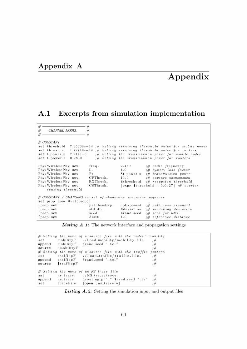
Appendix A
Appendix
A.1 Excerpts from simulation implementation
# ==================== ## CHANNEL MODEL ## ==================== #
# CONSTANTset th r e sho ld 7 .35638e−14 ;# Se t t i n g r e c e i v i n g t h r e s ho l d va lue f o r mobi le nodesset t h r e s h r t 1 .72719e−14 ;# Se t t i n g r e c e i v i n g t h r e s ho l d va lue f o r rou t e r sset t power n 7 .214e−3 ;# Se t t i n g the transmiss ion power f o r mobi le nodesset t power r 0 .2818 ;# Se t t i n g the transmiss ion power f o r rou t e r s
Phy/WirelessPhy set f r e q 2 . 4 e9 ;# radio frequencyPhy/WirelessPhy set L 1 . 0 ;# system l o s s f a c t o rPhy/WirelessPhy set Pt $t power n ;# transmiss ion powerPhy/WirelessPhy set CPThresh 10 . 0 ;# capture phenomenonPhy/WirelessPhy set RXThresh $ th re sho ld ;# recep t i on t h r e s ho l dPhy/WirelessPhy set CSThresh [ expr $ th re sho ld * 0 .0427 ] ;# ca r r i e r
sens ing t h r e s ho l d
# CONSTANT / CHANGING in s e t o f shadowing scenar io s sequenceset prop [ new $va l ( prop ) ]$prop set pathlossExp $pExponent ;# path l o s s exponent$prop set s td db $dev ia t i on ;# shadowing dev i a t i on$prop set s e ed $ rand seed ;# seed fo r RNG$prop set d i s t 0 1 . 0 ;# re f e r ence d i s t ance
Listing A.1: The network interface and propagation settings
# Se t t i n g the name of a˜ source f i l e with the nodes ’ mob i l i t yset mobi l i tyF . / Load mobi l i ty / m o b i l i t y f i l e ;#append mobi l i tyF $ rand seed ” . t c l ” ;#source $mobi l i tyF ;## Se t t i n g the name of a˜ source f i l e with the t r a f f i c pa t t e rnset t r a f f i c pF . / L o ad t r a f f i c / t r a f f i c f i l e ;#append t r a f f i c pF $ rand seed ” . t c l ” ;#source $ t r a f f i c pF ;#
# Se t t i n g the name of an NS trace f i l eset n s t r a c e . /NS trace / t r a c e ;#append n s t r a c e $ rout ing p ” ” $ rand seed ” . t r ” ;#set t r a c eF i l e [open $ns t r a c e w] ;#
Listing A.2: Setting the simulation input and output files
60
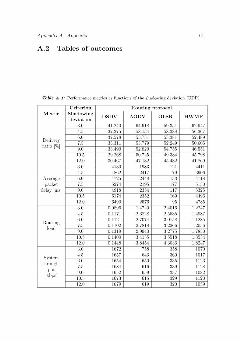
Appendix A. Appendix 61
A.2 Tables of outcomes
Table A.1: Performance metrics as functions of the shadowing deviation (UDP)
MetricCriterion Routing protocol
Shadowingdeviation
DSDV AODV OLSR HWMP
Deliveryratio [%]
3.0 41.240 64.918 59.351 62.9474.5 37.275 58.134 58.388 56.3676.0 37.578 53.731 53.381 52.4897.5 35.311 53.779 52.249 50.6059.0 33.490 52.820 54.755 46.55110.5 29.268 50.725 49.384 45.79812.0 30.467 47.132 45.432 41.869
Averagepacket
delay [ms]
3.0 4130 1983 121 44114.5 4862 2417 79 39066.0 4725 2448 133 47187.5 5274 2195 177 51309.0 4918 2354 117 532510.5 6174 2352 169 449612.0 6490 2576 95 4785
Routingload
3.0 0.0896 1.4720 2.4016 1.22474.5 0.1171 2.3828 2.5535 1.49876.0 0.1121 2.7074 3.0158 1.12857.5 0.1102 2.7818 3.2266 1.20569.0 0.1319 2.9940 3.2775 1.785010.5 0.1400 3.4135 3.5518 1.353412.0 0.1448 3.8454 4.3036 1.8247
Systemthrough-
put[kbps]
3.0 1672 758 358 10704.5 1657 643 360 10176.0 1654 650 335 11237.5 1684 616 339 11289.0 1652 659 337 108210.5 1673 615 329 112012.0 1679 619 320 1059

Appendix A. Appendix 62
Table A.2: Performance metrics as functions of the path loss exponent (UDP)
MetricCriterion Routing protocolPath lossexponent
DSDV AODV OLSR HWMP
Deliveryratio [%]
2.0 58.052 80.441 81.285 84.9712.4 52.610 75.829 78.195 67.7242.8 41.179 67.550 56.583 61.3213.2 38.934 51.903 46.030 47.8333.6 29.358 45.285 43.495 41.0764.0 29.676 39.209 39.418 38.3794.4 19.179 26.574 24.447 31.218
Averagepacket
delay [ms]
2.0 4768 976 14 3362.4 4593 1130 15 22582.8 3986 1789 67 33063.2 3643 2707 237 43893.6 3530 2632 2819 58854.0 3418 2690 4042 67444.4 3236 3244 4691 7353
Routingload
2.0 0.0510 0.4705 2.7678 1.13792.4 0.0696 1.2285 2.8248 0.92582.8 0.0893 2.1030 2.7662 1.07393.2 0.1465 3.3598 2.4914 1.34673.6 0.2706 4.1870 1.3196 1.70594.0 0.4465 4.4548 1.1801 1.43644.4 0.8055 5.9988 1.1908 1.4387
Systemthrough-
put[kbps]
2.0 1575 929 208 8502.4 1576 770 212 10062.8 1545 707 291 10133.2 1410 662 471 12083.6 1448 703 1076 14074.0 1340 818 1218 16504.4 1493 870 1265 1648
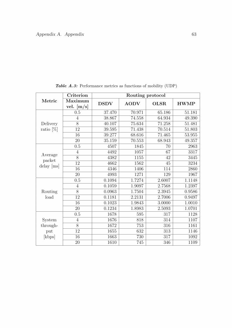
Appendix A. Appendix 63
Table A.3: Performance metrics as functions of mobility (UDP)
MetricCriterion Routing protocolMaximumvel. [m/s]
DSDV AODV OLSR HWMP
Deliveryratio [%]
0.5 37.470 70.971 65.186 51.1814 38.867 74.558 64.934 49.3908 40.107 75.634 71.258 51.48112 39.595 71.438 70.514 51.80316 39.277 68.616 71.465 53.95520 35.159 70.553 68.943 49.357
Averagepacket
delay [ms]
0.5 4507 1845 70 29634 4492 1057 67 33178 4382 1155 42 344512 4662 1562 45 323416 4346 1406 114 286020 4993 1271 129 1967
Routingload
0.5 0.1094 1.7274 2.6007 1.11484 0.1059 1.9097 2.7568 1.23978 0.0963 1.7504 2.3945 0.958612 0.1181 2.2131 2.7006 0.949716 0.1023 1.9843 3.0000 1.001020 0.1234 1.8983 2.5093 1.0701
Systemthrough-
put[kbps]
0.5 1678 595 317 11284 1676 818 314 11078 1672 753 316 116112 1655 632 313 114616 1663 730 317 109220 1610 745 346 1109
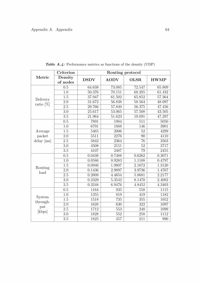
Appendix A. Appendix 64
Table A.4: Performance metrics as functions of the density (UDP)
MetricCriterion Routing protocolDensityof nodes
DSDV AODV OLSR HWMP
Deliveryratio [%]
0.5 64.638 73.085 72.547 65.8091.0 50.376 70.151 68.285 61.4321.5 37.947 61.502 65.852 57.3642.0 31.672 56.838 58.564 48.0972.5 29.766 57.840 56.375 47.4563.0 25.617 53.065 57.508 43.5053.5 21.964 51.623 19.091 47.297
Averagepacket
delay [ms]
0.5 7891 1984 511 50501.0 6791 1888 146 39011.5 5465 2006 52 42992.0 5511 2276 90 41102.5 5842 2364 76 35633.0 4508 2151 52 37173.5 4107 2487 79 2455
Routingload
0.5 0.0438 0.7488 0.6262 0.30711.0 0.0586 0.9283 1.1108 0.47971.5 0.0946 1.9807 2.1672 1.31202.0 0.1436 2.9897 3.9736 1.47672.5 0.2008 4.4654 5.8681 2.21773.0 0.2329 5.3542 8.1470 2.40823.5 0.3248 6.9476 4.8452 4.3403
Systemthrough-
put[kbps]
0.5 1164 935 558 11151.0 1355 819 419 11821.5 1518 735 355 10522.0 1628 630 322 10972.5 1712 553 248 10993.0 1828 552 258 11123.5 1825 457 211 990
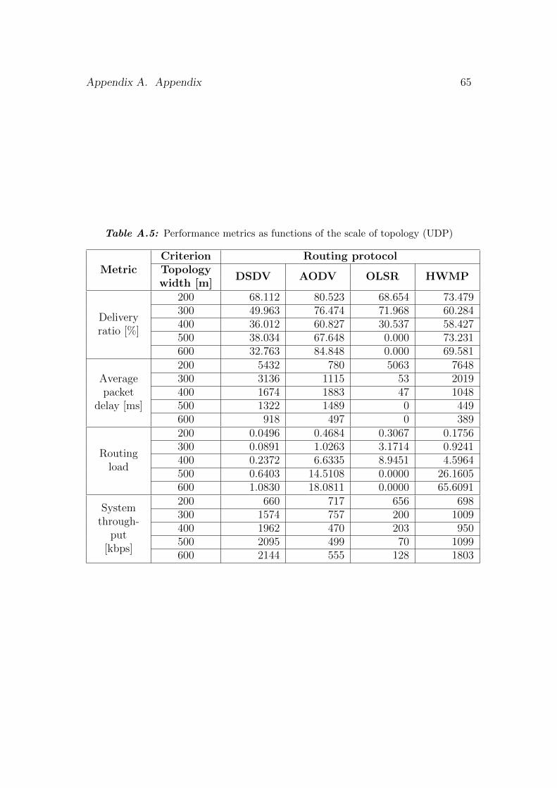
Appendix A. Appendix 65
Table A.5: Performance metrics as functions of the scale of topology (UDP)
MetricCriterion Routing protocolTopologywidth [m]
DSDV AODV OLSR HWMP
Deliveryratio [%]
200 68.112 80.523 68.654 73.479300 49.963 76.474 71.968 60.284400 36.012 60.827 30.537 58.427500 38.034 67.648 0.000 73.231600 32.763 84.848 0.000 69.581
Averagepacket
delay [ms]
200 5432 780 5063 7648300 3136 1115 53 2019400 1674 1883 47 1048500 1322 1489 0 449600 918 497 0 389
Routingload
200 0.0496 0.4684 0.3067 0.1756300 0.0891 1.0263 3.1714 0.9241400 0.2372 6.6335 8.9451 4.5964500 0.6403 14.5108 0.0000 26.1605600 1.0830 18.0811 0.0000 65.6091
Systemthrough-
put[kbps]
200 660 717 656 698300 1574 757 200 1009400 1962 470 203 950500 2095 499 70 1099600 2144 555 128 1803
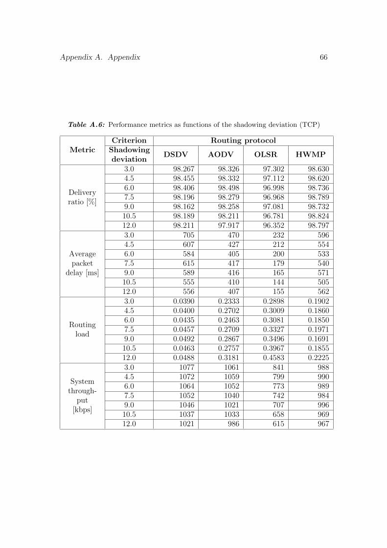
Appendix A. Appendix 66
Table A.6: Performance metrics as functions of the shadowing deviation (TCP)
MetricCriterion Routing protocol
Shadowingdeviation
DSDV AODV OLSR HWMP
Deliveryratio [%]
3.0 98.267 98.326 97.302 98.6304.5 98.455 98.332 97.112 98.6206.0 98.406 98.498 96.998 98.7367.5 98.196 98.279 96.968 98.7899.0 98.162 98.258 97.081 98.73210.5 98.189 98.211 96.781 98.82412.0 98.211 97.917 96.352 98.797
Averagepacket
delay [ms]
3.0 705 470 232 5964.5 607 427 212 5546.0 584 405 200 5337.5 615 417 179 5409.0 589 416 165 57110.5 555 410 144 50512.0 556 407 155 562
Routingload
3.0 0.0390 0.2333 0.2898 0.19024.5 0.0400 0.2702 0.3009 0.18606.0 0.0435 0.2463 0.3081 0.18507.5 0.0457 0.2709 0.3327 0.19719.0 0.0492 0.2867 0.3496 0.169110.5 0.0463 0.2757 0.3967 0.185512.0 0.0488 0.3181 0.4583 0.2225
Systemthrough-
put[kbps]
3.0 1077 1061 841 9884.5 1072 1059 799 9906.0 1064 1052 773 9897.5 1052 1040 742 9849.0 1046 1021 707 99610.5 1037 1033 658 96912.0 1021 986 615 967
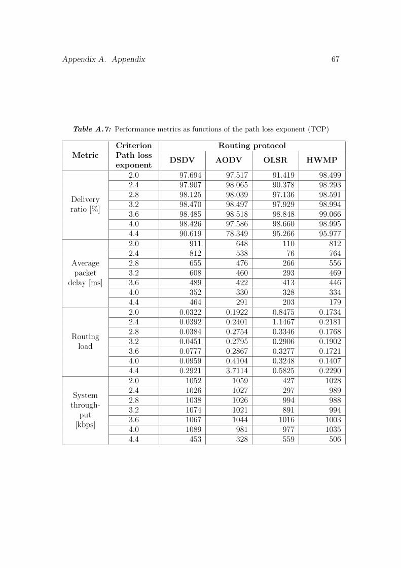
Appendix A. Appendix 67
Table A.7: Performance metrics as functions of the path loss exponent (TCP)
MetricCriterion Routing protocolPath lossexponent
DSDV AODV OLSR HWMP
Deliveryratio [%]
2.0 97.694 97.517 91.419 98.4992.4 97.907 98.065 90.378 98.2932.8 98.125 98.039 97.136 98.5913.2 98.470 98.497 97.929 98.9943.6 98.485 98.518 98.848 99.0664.0 98.426 97.586 98.660 98.9954.4 90.619 78.349 95.266 95.977
Averagepacket
delay [ms]
2.0 911 648 110 8122.4 812 538 76 7642.8 655 476 266 5563.2 608 460 293 4693.6 489 422 413 4464.0 352 330 328 3344.4 464 291 203 179
Routingload
2.0 0.0322 0.1922 0.8475 0.17342.4 0.0392 0.2401 1.1467 0.21812.8 0.0384 0.2754 0.3346 0.17683.2 0.0451 0.2795 0.2906 0.19023.6 0.0777 0.2867 0.3277 0.17214.0 0.0959 0.4104 0.3248 0.14074.4 0.2921 3.7114 0.5825 0.2290
Systemthrough-
put[kbps]
2.0 1052 1059 427 10282.4 1026 1027 297 9892.8 1038 1026 994 9883.2 1074 1021 891 9943.6 1067 1044 1016 10034.0 1089 981 977 10354.4 453 328 559 506
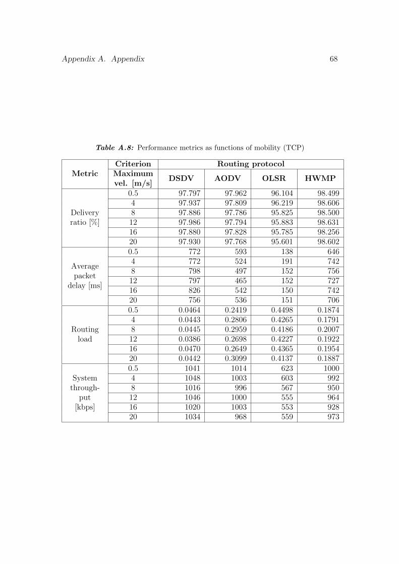
Appendix A. Appendix 68
Table A.8: Performance metrics as functions of mobility (TCP)
MetricCriterion Routing protocolMaximumvel. [m/s]
DSDV AODV OLSR HWMP
Deliveryratio [%]
0.5 97.797 97.962 96.104 98.4994 97.937 97.809 96.219 98.6068 97.886 97.786 95.825 98.50012 97.986 97.794 95.883 98.63116 97.880 97.828 95.785 98.25620 97.930 97.768 95.601 98.602
Averagepacket
delay [ms]
0.5 772 593 138 6464 772 524 191 7428 798 497 152 75612 797 465 152 72716 826 542 150 74220 756 536 151 706
Routingload
0.5 0.0464 0.2419 0.4498 0.18744 0.0443 0.2806 0.4265 0.17918 0.0445 0.2959 0.4186 0.200712 0.0386 0.2698 0.4227 0.192216 0.0470 0.2649 0.4365 0.195420 0.0442 0.3099 0.4137 0.1887
Systemthrough-
put[kbps]
0.5 1041 1014 623 10004 1048 1003 603 9928 1016 996 567 95012 1046 1000 555 96416 1020 1003 553 92820 1034 968 559 973
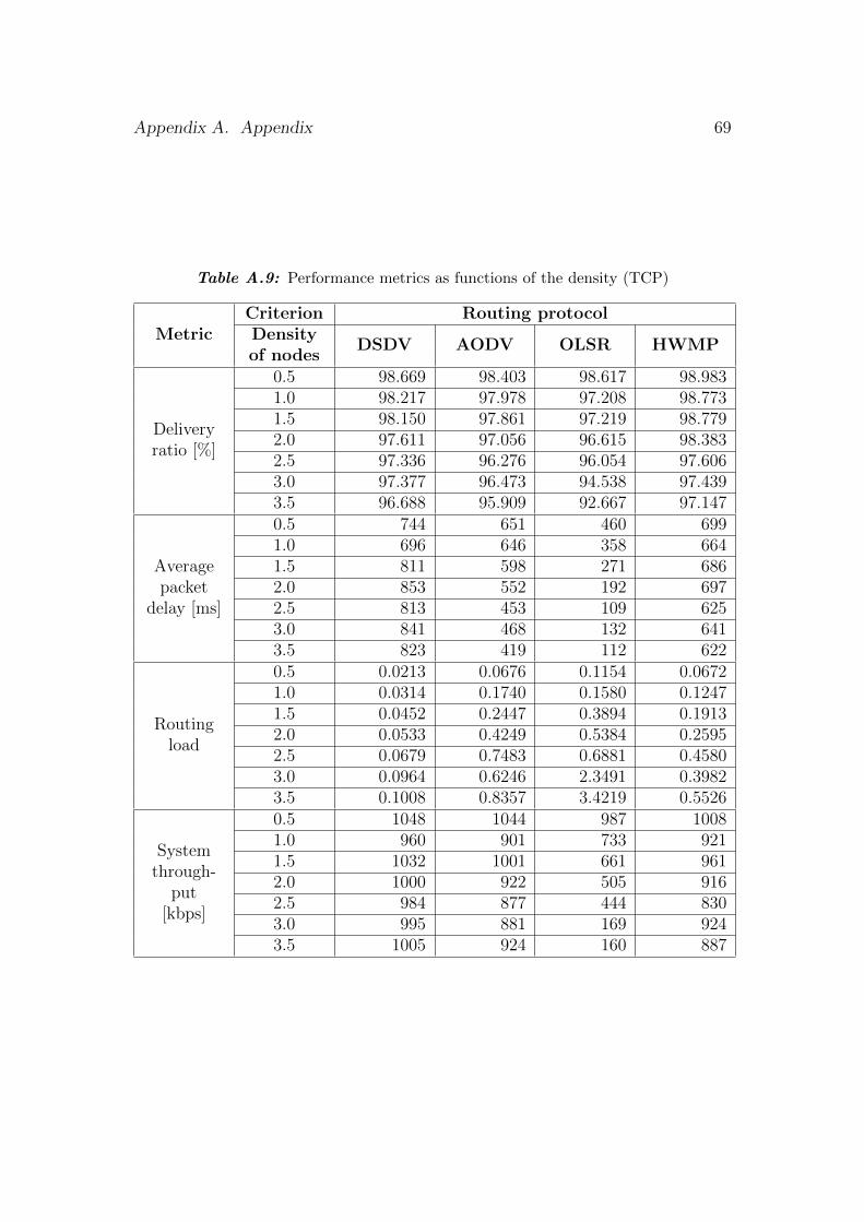
Appendix A. Appendix 69
Table A.9: Performance metrics as functions of the density (TCP)
MetricCriterion Routing protocolDensityof nodes
DSDV AODV OLSR HWMP
Deliveryratio [%]
0.5 98.669 98.403 98.617 98.9831.0 98.217 97.978 97.208 98.7731.5 98.150 97.861 97.219 98.7792.0 97.611 97.056 96.615 98.3832.5 97.336 96.276 96.054 97.6063.0 97.377 96.473 94.538 97.4393.5 96.688 95.909 92.667 97.147
Averagepacket
delay [ms]
0.5 744 651 460 6991.0 696 646 358 6641.5 811 598 271 6862.0 853 552 192 6972.5 813 453 109 6253.0 841 468 132 6413.5 823 419 112 622
Routingload
0.5 0.0213 0.0676 0.1154 0.06721.0 0.0314 0.1740 0.1580 0.12471.5 0.0452 0.2447 0.3894 0.19132.0 0.0533 0.4249 0.5384 0.25952.5 0.0679 0.7483 0.6881 0.45803.0 0.0964 0.6246 2.3491 0.39823.5 0.1008 0.8357 3.4219 0.5526
Systemthrough-
put[kbps]
0.5 1048 1044 987 10081.0 960 901 733 9211.5 1032 1001 661 9612.0 1000 922 505 9162.5 984 877 444 8303.0 995 881 169 9243.5 1005 924 160 887
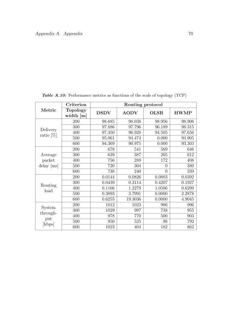
Appendix A. Appendix 70
Table A.10: Performance metrics as functions of the scale of topology (TCP)
MetricCriterion Routing protocolTopologywidth [m]
DSDV AODV OLSR HWMP
Deliveryratio [%]
200 98.685 98.038 98.956 98.906300 97.886 97.796 96.189 98.315400 97.450 96.928 94.505 97.656500 95.061 94.474 0.000 94.905600 94.369 90.975 0.000 93.303
Averagepacket
delay [ms]
200 678 541 569 646300 639 387 205 612400 756 289 172 408500 720 304 0 380600 738 240 0 339
Routingload
200 0.0144 0.0826 0.0803 0.0392300 0.0439 0.3114 0.4207 0.1927400 0.1166 1.2279 1.0586 0.6299500 0.3893 3.7991 0.0000 2.2878600 0.6255 19.3036 0.0000 4.9045
Systemthrough-
put[kbps]
200 1012 1023 986 996300 1029 997 738 955400 978 770 500 903500 950 525 98 792600 1023 404 182 862
List of Figures
3.1 Classification of multi-hop wireless networks [11] . . . . . . . . . . 73.2 The backbone type of WMN topology . . . . . . . . . . . . . . . . 83.3 The client type of WMN topology . . . . . . . . . . . . . . . . . . 83.4 The hybrid type of WMN topology . . . . . . . . . . . . . . . . . 93.5 The mechanism of MPR flooding in the OLSR protocol . . . . . . 20
4.1 Probability of receiving a packet - shadowing model . . . . . . . . 274.2 Probability of receiving a packet - two ray ground model . . . . . 274.3 BPMN diagram of the simulation running process outline . . . . . 30
5.1 Outcomes interpretation for rural and urban areas . . . . . . . . . 345.2 Delivery ratio as a function of the shadowing deviation (UDP) . . 365.3 End to end delay as a function of the shadowing deviation (UDP) 365.4 Routing load as a function of the shadowing deviation (UDP) . . 365.5 System throughput as a function of the shadowing deviation (UDP) 365.6 Delivery ratio as a function of the path loss exponent (UDP) . . . 385.7 End to end delay as a function of the path loss exponent (UDP) . 385.8 Routing load as a function of the path loss exponent (UDP) . . . 385.9 System throughput as a function of the path loss exponent (UDP) 385.10 Delivery ratio as a function of nodes’ velocity (UDP) . . . . . . . 415.11 End to end delay as a function of nodes’ velocity (UDP) . . . . . 415.12 Routing load as a function of nodes’ velocity (UDP) . . . . . . . . 415.13 System throughput as a function of nodes’ velocity (UDP) . . . . 415.14 Delivery ratio as a function of nodes’ density (UDP) . . . . . . . . 425.15 End to end delay as a function of nodes’ density (UDP) . . . . . . 425.16 Routing load as a function of nodes’ density (UDP) . . . . . . . . 435.17 System throughput as a function of nodes’ density (UDP) . . . . 435.18 Delivery ratio as a function of the topology scale (UDP) . . . . . 445.19 End to end delay as a function of the topology scale (UDP) . . . 445.20 Routing load as a function of the topology scale (UDP) . . . . . . 445.21 System throughput as a function of the topology scale (UDP) . . 445.22 Delivery ratio as a function of the shadowing deviation (TCP) . . 455.23 End to end delay as a function of the shadowing deviation (TCP) 455.24 Routing load as a function of the shadowing deviation (TCP) . . 45
71
List of Figures 72
5.25 System throughput as a function of the shadowing deviation (TCP) 455.26 Delivery ratio as a function of the path loss exponent (TCP) . . 465.27 End to end delay as a function of the path loss exponent (TCP) . 465.28 Routing load as a function of the path loss exponent (TCP) . . . 475.29 System throughput as a function of the path loss exponent (TCP) 475.30 Delivery ratio as a function of nodes’ velocity (TCP) . . . . . . . 485.31 End to end delay as a function of nodes’ velocity (TCP) . . . . . 485.32 Routing load as a function of nodes’ velocity (TCP) . . . . . . . . 485.33 System throughput as a function of nodes’ velocity (TCP) . . . . 485.34 Delivery ratio as a function of nodes’ density (TCP) . . . . . . . . 495.35 End to end delay as a function of nodes’ density (TCP) . . . . . . 495.36 Routing load as a function of nodes’ density (TCP) . . . . . . . . 495.37 System throughput as a function of nodes’ density (TCP) . . . . . 495.38 Delivery ratio as a function of the topology scale (TCP) . . . . . 505.39 End to end delay as a function of the topology scale (TCP) . . . . 505.40 Routing load as a function of the topology scale (TCP) . . . . . . 505.41 System throughput as a function of the topology scale (TCP) . . 50

List of Tables
4.1 Typical values of path loss exponent β . . . . . . . . . . . . . . . 284.2 Typical values of shadowing deviation σdB . . . . . . . . . . . . . 28
A.1 Performance metrics as functions of the shadowing deviation (UDP) 61A.2 Performance metrics as functions of the path loss exponent (UDP) 62A.3 Performance metrics as functions of mobility (UDP) . . . . . . . . 63A.4 Performance metrics as functions of the density (UDP) . . . . . . 64A.5 Performance metrics as functions of the scale of topology (UDP) . 65A.6 Performance metrics as functions of the shadowing deviation (TCP) 66A.7 Performance metrics as functions of the path loss exponent (TCP) 67A.8 Performance metrics as functions of mobility (TCP) . . . . . . . . 68A.9 Performance metrics as functions of the density (TCP) . . . . . . 69A.10 Performance metrics as functions of the scale of topology (TCP) . 70
73
Nomenclature
ns Network Simulator version 2.34AODV Ad hoc On-Demand Distance Vector Routing ProtocolARP Address Resolution ProtocolBF Bellman FordCSMA/CA Carrier Sense Multiple Access with Collision AvoidanceDCF Distributed Coordination FunctionDSDV Destination-Sequenced Distance-Vector Routing ProtocolETT Expected Transmission Time MetricETX Expected Transmission Count MetricGB Gafni-Bertsekas routing algorithmHWMP Hybrid Wireless Mesh ProtocolIEEE Institute of Electrical and Electronics EngineersIETF Internet Engineering Task ForceIP Internet ProtocolISO International Organization for StandardizationLL Link LayerLMR Lightweight Mobile Routing algorithmLSR Link State RoutingMAC Media Access ControlMANET Mobile Ad-hoc NetworksMIMO Multiple-Input and Multiple-Output AntennasMPR Multipoint RelayOFDM Orthogonal Frequency Division MultiplexingOLSR Optimized Link State Routing ProtocolOSI Open System InterconnectionPC Personal ComputerPDA Personal Digital AssistantRANN Root Announcement routing messageRERR Route Error routing messageRFC Request for CommentsRIP Routing Internet ProtocolRM Reference ModelRREP Route Reply routing messageRREQ Route Requests routing message
74

Nomenclature 75
RTT Round Trip Time MetricTC Topology Control routing messageTCP Transmission Control ProtocolTDMA Time Division Multiple AccessTORA Temporally-Ordered Routing AlgorithmTTL Time To LiveUWB Ultra Wide BandWLAN Wireless Local Area NetworksWMN Wireless Mesh Network

References
[1] IEEE Standard for Information Technology-Telecommunications and Infor-mation Exchange Between Systems-Local and Metropolitan Area Networks-Specific Requirements - Part 11: Wireless LAN Medium Access Control(MAC) and Physical Layer (PHY) Specifications, 2007. IEEE Std 802.11-2007 (Revision of IEEE Std 802.11-1999).
[2] I. F. Akyildiz and Xudong Wang. A survey on wireless mesh networks. 2005.
[3] A. Boukerche, L. Guardalben, J. B. M. Sobral, and M. S. M. A. Notare. Aself-x approach for OLSR routing protocol in large-scale wireless mesh net-works. In Proc. IEEE Global Telecommunications Conf. IEEE GLOBECOM2008, pages 1–6, 2008.
[4] J. Brugge, L. Paquereau, and P. E. Heegaard. Experience report on imple-menting and simulating a routing protocol in ns-2 and ns-3. In Proc. SecondInt Advances in System Simulation (SIMUL) Conf, pages 88–93, 2010.
[5] T. Clausen and P. Jacquet. Optimized link state routing protocol (OLSR),RFC 3626, IETF. 2003.
[6] M. Cornils, M. Bahr, and T. Gamer. Simulative analysis of the hybridwireless mesh protocol (HWMP). In Proc. European Wireless Conf. (EW),pages 536–543, 2010.
[7] G. Elias, M. Novaes, G. Cavalcanti, and D. Porto. Simulation-based perfor-mance evaluation of the SNDP protocol for infrastructure WMNs. In Proc.24th IEEE Int Advanced Information Networking and Applications (AINA)Conf, pages 90–97, 2010.
[8] Q. Feng, Z. Cai, J. Yang, and X. Hu. A performance comparison of the adhoc network protocols. In Proc. Second Int. Workshop Computer Scienceand Engineering WCSE ’09, volume 2, pages 293–297, 2009.
[9] The Working Group for WLAN Standards of the IEEE. HWMP protocolspecification. 2006.
76
References 77
[10] B. K. Gupta, B. M. Acharya, and M. K. Mishra. Optimization of routingalgorithm in wireless mesh networks. In Proc. World Congress Nature &Biologically Inspired Computing NaBIC 2009, pages 1150–1155, 2009.
[11] B. S. Manoj and R. R. Rao. Wireless mesh networks: Issues and solutions.In Wireless Mesh Networks: Architectures, Protocols, and Standards. Y.S.Zhang, et al., Eds., Florida: CRC Press, 2006.
[12] N. H. Moleme, M. O. Odhiambo, and A. M. Kurien. Enhancing video stream-ing in 802.11 wireless mesh networks using two-layer mechanism solution. InProc. AFRICON ’09. AFRICON, pages 1–6, 2009.
[13] W. A. Moreira, R. Lopes Gomes, and A. J. Gomes Abelem. A multiple-metric approach for routing in wireless mesh networks. In Proc. IEEE Int.Symp. a World of Wireless, Mobile and Multimedia Networks & WorkshopsWoWMoM 2009, pages 1–6, 2009.
[14] Wireless Software R&D Group of IITP RAS. HWMP model for NS-2. Inhttps://forge.iitp.ru/ns2/hwmp/hwmp ns2, Cited May 2011.
[15] V. Park and S. Corson. Temporally-ordered routing algorithm (TORA) ver-sion 1 functional specification, IETF internet draft. 1997.
[16] V. D. Park and M. S. Corson. A highly adaptive distributed routing algo-rithm for mobile wireless networks. In Proc. IEEE Sixteenth Annual JointConf. of the IEEE Computer and Communications Societies INFOCOM ’97,volume 3, pages 1405–1413, 1997.
[17] C. Perkins, E. Royer, and S. Das. Ad hoc on-demand distance vector (AODV)routing, RFC 3561, IETF. 2003.
[18] C. E. Perkins and P. Bhagwat. Highly dynamic destination sequenced dis-tance vector routing (DSDV) for mobile computers. 1994.
[19] C. E. Perkins and E. M. Royer. Ad-hoc on-demand distance vector routing.In Proc. Second IEEE Workshop Mobile Computing Systems and Applica-tions WMCSA ’99, pages 90–100, 1999.
[20] C. E. Perkins, E. M. Royer, S. R. Das, and M. K. Marina. Performancecomparison of two on-demand routing protocols for ad hoc networks. IEEEPersonal Communications, 8(1):16–28, 2001.
[21] F. J. Ros. UM-OLSR docuentation. In http://masimum.dif.um.es/um-olsr/html/, Cited May 2011.

References 78
[22] M. P. Tahiliani, K. C. Shet, and T. G. Basavaraju. Performance evaluationof tcp variants over routing protocols in multi-hop wireless networks. InProc. Int Computer and Communication Technology (ICCCT) Conf, pages387–392, 2010.
[23] M. Umlauft and P. Reichl. Experiences with the ns-2 network simulator -explicitly setting seeds considered harmful. In Proc. Wireless Telecommuni-cations Symp. WTS 2007, pages 1–5, 2007.
[24] The CMU Monarch Project. The CMU monarch projects wireless and mo-bility extensions to ns. 1999.
[25] The VINT Project. The ns Manual (formerly ns Notes and Documentation).2010.
[26] K. Ur Rahman Khan, A. V. Reddy, R. U. Zaman, K. A. Reddy, and T. S.Harsha. An efficient DSDV routing protocol for wireless mobile ad hoc net-works and its performance comparison. In Proc. Second UKSIM EuropeanSymp. Computer Modeling and Simulation EMS ’08, pages 506–511, 2008.
[27] A. Zakrzewska, L. Koszalka, and I. Pozniak-Koszalka. Performance studyof routing protocols for wireless mesh networks. In Proc. 19th Int. Conf.Systems Engineering ICSENG ’08, pages 331–336, 2008.
[28] Y. Zhang, J. Luo, and H. Hu, editors. Wireless mesh networking, Architec-tures, Protocols and Standards. Auerbach Publications, 2007.