SIAM J. DISC. MATH.Vol. 2, No. 4, pp. 508-523, November 1989

(C) 1989 Society for Industrial and Applied Mathematics009

AVERAGE PERFORMANCE OF HEURISTICS FOR SATISFIABILITY*

RAJEEV KOHLI]" AND RAMESH KRISHNAMURTIzl:

Abstract. Distribution-free tight lower bounds on the average performance ratio for random search, for agreedy heuristic and for a probabilistic greedy heuristic are derived for an optimization version of satisfiability.On average, the random solution is never worse than ofthe optimal, regardless ofthe data-generating distribution.The lower bound on the average greedy solution is at least of the optimal, and this bound increases with theprobability of the greedy heuristic selecting the optimal at each step. In the probabilistic greedy heuristic, prob-abilities are introduced into the search strategy so that a decrease in the probability of finding the optimalsolution occurs only if the nonoptimal solution becomes closer to the optimal. Across problem instances, andregardless of the distribution giving rise to data, the minimum average value of the solutions identified by theprobabilistic greedy heuristic is no less than of the optimal.

Key words, satisfiability, greedy heuristics, probabilistic heuristics, average performance

AMS(MOS) subject classification. 68Q25

1. Introduction. This paper examines the average performance of random search,ofa greedy heuristic and ofa probabilistic version ofa greedy heuristic for an optimizationversion of satisfiability. We derive tight lower bounds on the average performance ofeach heuristic. The analysis assumes no specific data-generating distributions and thereforeis valid for all distributions.

A variety of analytic approaches have recently been pursued to analyze the average-case performance of heuristics. These include representing the execution of algorithmsby Markov chains (Coffman, Leuker, and Rinnooy Kan 5 ), obtaining the performancebound for a more tractable function that dominates the performance of the heuristic foreach problem instance (Bruno and Downey [3 ], Boxma [2 ]), and obtaining the per-formance bound for a simpler, more easily analyzed heuristic which dominates the heu-ristic of interest for each problem instance (Csirik et al. [6 ). Bounds that hold for mostproblem instances have also been employed to obtain asymptotic bounds for the average-case performance of various heuristics (Bentley et al. [1] and Coffman and Leighton4 ]). A number of results from applied probability theory have been used for average-

case analyses by Frenk and Rinnooy Kan 10], Karp, Luby, and Marchetti-Spaccamela14 ], Shor 17 ], and Leighton and Shor 15 ]. The vast majority of these approaches

begins by assuming independent, identically distributed data from a given density function.The subsequent analyses are often difficult, and one rarely finds an explicit formula forthe quantity of interest. One reason for this is that conditional probabilities arise in theanalyses, and after a sufficient number of steps, the conditioning can make the analysesformidable. Appropriate choice of distributional assumptions also is difficult, as are in-ferences regarding the robustness of results for a given distribution to other distributions.

A well-known algorithm for solving satisfiability is the Davis-Putnam Procedure(Davis, Logemann, and Loveland 7 ). Goldberg, Purdom, and Brown 11 ], and Francoand Paull [9] have analyzed the average-case complexity of variants of this procedurefor solving satisfiability. Johnson 13 considers an optimization version of satisfiability,called maximum satisfiability, proposes two heuristics for solving the maximum satisfi-ability problem, and proves tight worst-case bounds on the performances of these heu-

Received by the editors December 15, 1988; accepted for publication February 28, 1989. This researchwas supported by the Natural Sciences and Engineering Research Council ofCanada under grant OGP0036809.

f Graduate School of Business, University of Pittsburgh, Pittsburgh, Pennsylvania 15260.School ofComputing Science, Simon Fraser University, Burnaby, British Columbia, V5A 1S6, Canada.

508

PERFORMANCE OF HEURISTICS 509

ristics. One of these heuristics is the greedy heuristic that we use in this paper. If eachclause contains at least variables, Johnson [13 shows a tight worst-case bound ofl/(l + for the greedy heuristic. Since we consider the most general optimization versionof satisfiability, where unary clauses (clauses with just one variable) are allowed, thisbound reduces to 1/2. As one ofour results, we derive this bound using a different approach.Lieberherr and Specker 16 provide the best possible polynomial-time algorithm for themaximum satisfiability problem where unary clauses are allowed, but the set of clausesmust be 2-satisfiable, i.e., any two ofthe clauses are simultaneously satisfiable. The lowerbound obtained for their algorithm is 0.618.

In the present analyses, we consider the lower bound of the average performancemaking no assumption regarding the data-generating distribution. For two of the threeprocedures (random search and the probabilistic greedy heuristic), we also make noassumption regarding the independence of data. For the third (the greedy heuristic), weassume independence, but only in a certain "aggregate" sense, which we discuss later.Each ofthe bounds we obtain is tight. Our central results are as follows. Random search,which has an arbitrarily bad performance in the worst case, provides solutions that, onaverage, are never worse than 1/2 of the optimal. The greedy heuristic can potentiallyimprove on this performance. Although the lower bound on its average performanceratio can be 1/2 of the optimal, this lower bound increases with the probability of theheuristic selecting the optimal at each step. A probabilistic algorithm related to the greedyheuristic is then described. The probabilities are introduced into the search strategy sothat a decrease in the probability of finding the optimal solution occurs only if the non-optimal solution becomes closer to the optimal. The search probabilities are not fixeda priori but exploit the structure ofthe data to force a trade-off for every problem instance.Across problem instances, and regardless of the distribution giving rise to the data, theaverage performance of the algorithm is never less than of the optimal.

Section 2 describes the maximum satisfiability problem, the random search pro-cedure, and obtains a tight lower bound on its average performance. Section 3 introducesthe greedy heuristic, derives its worst-case bound, and a tight lower bound on its averageperformance. Section 4 describes the probabilistic greedy heuristic and derives a tightlower bound on its average performance.

2. The Msat problem. Consider the following optimization version of satisfiability:given n clauses, each described by a disjunction ofa subset ofk variables or their negations,find a truth assignment for the variables that maximizes the number of clauses satisfied.The above problem, which is the most general version of maximum satisfiability, is NP-complete (Johnson 13 ). We call this Msat.

We use the following tabular representation of Msat. For a problem involving nclauses and k variables, construct a table Tk with n rows and 2k columns. The ith rowis associated with clause i, 1, n. A pair of columns, uj, z, is associated with thejth variable, j 1, k. Let tij denote the entry in the cell identified by row andcolumn u, and let ti denote the entry in the cell identified by row and column z. For

1, n,j 1, k, define

o 1, ti 0, if clause contains variable j,

ti O, tij 1, if clause contains the negation of variable j,

o O, ti 0, if clause contains neither variable j nor its negation.

A truth assignment for satisfiability results in the jth variable being assigned a T(True) or an F (False), j 1, k. This corresponds to selecting either column u

510 RAJEEV KOHLI AND RAMESH KRISHNAMURTI

(if the jth variable is assigned a T) or (if the jth variable is assigned an F), j1, k, for Msat. Consequently, selecting uj or tb for each j, j 1, k, such thatthe maximum number of rows in these columns have at least one 1, corresponds tosolving Msat for Tk; i.e., finding a truth assignment that maximizes the number ofclausessatisfied.

Let T(uk)(T(k)) denote the table obtained by deleting from T all rows with ain column u(), and deleting both u and zTk. Let the resulting table be denoted T_ 1.

That is,

if column ug is chosen from Tk,T_

T(zTk), if column zTg is chosen from T.

In general, let T( uj)( T(fla)) denote the table obtained by deleting from T all rowswith a in column uj(zT), and deleting both uj and z, j 1, k. Let the resultingtable be denoted T_ 1. That is,

T(u), if column uj. is chosen from T,T_

T(ff), if column ff is chosen from Tj..

Let xj denote the number of ’s in u and let nj denote the total number of ’s acrosscolumns uj and in table T, j 1, k. Without loss of generality, assume that thecolumns u, j 1, k, comprise the optimal solution for Msat described by T. Letm denote the optimal solution to Msat described by Tk. In general, let m denotethe value of the optimal solution to Msat described by Tj., j 1, ..., k. Also, leta() denote the value of the optimal solution to Msat described by T(uj)(T()), j1, ..., k. That is,

a, if column u is chosen from T,m_

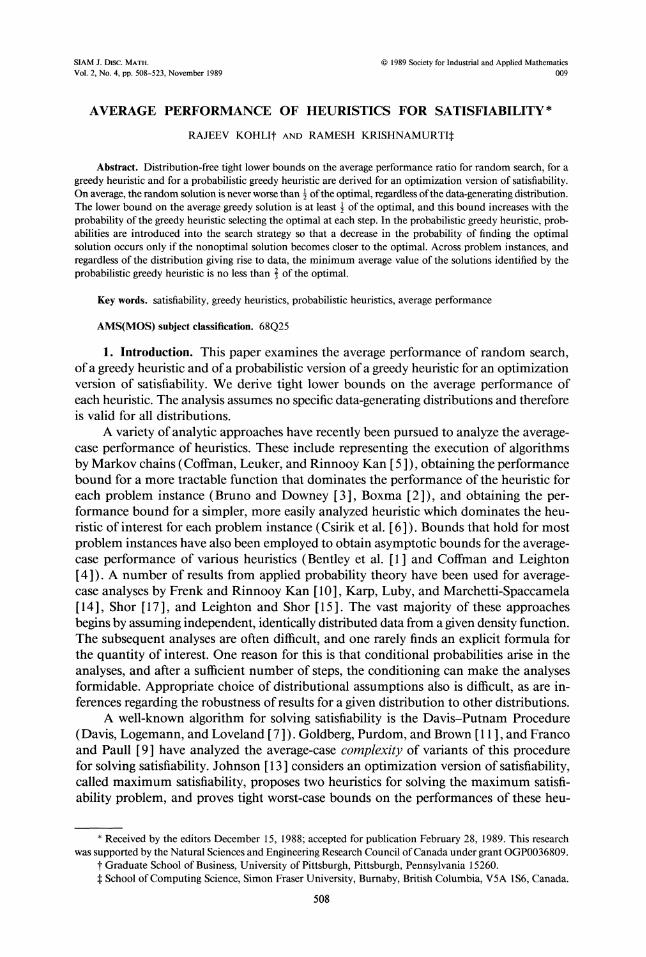
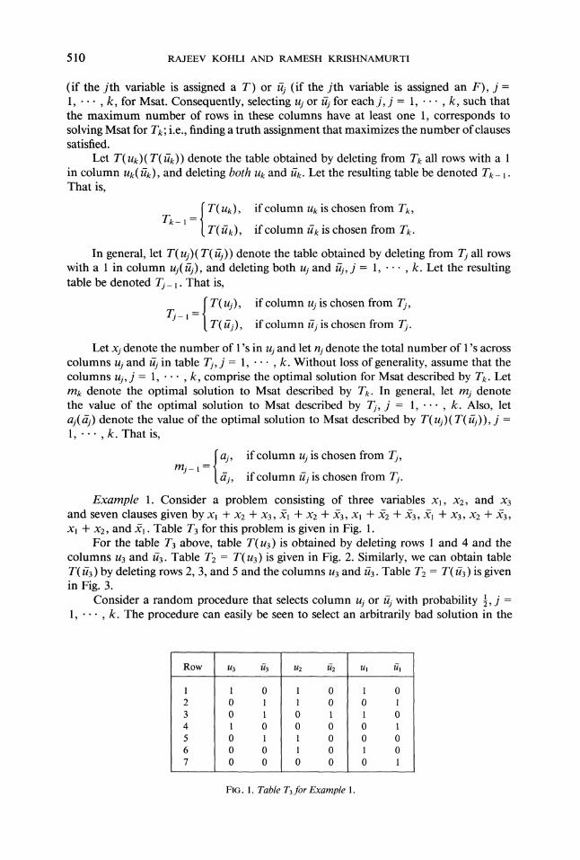
Tj., if column ffj is chosen from T.Example 1. Consider a problem consisting of three variables Xl, x2, and x3

and seven clauses given byxl + xz, and 1. Table T3 for this problem is given in Fig. 1.

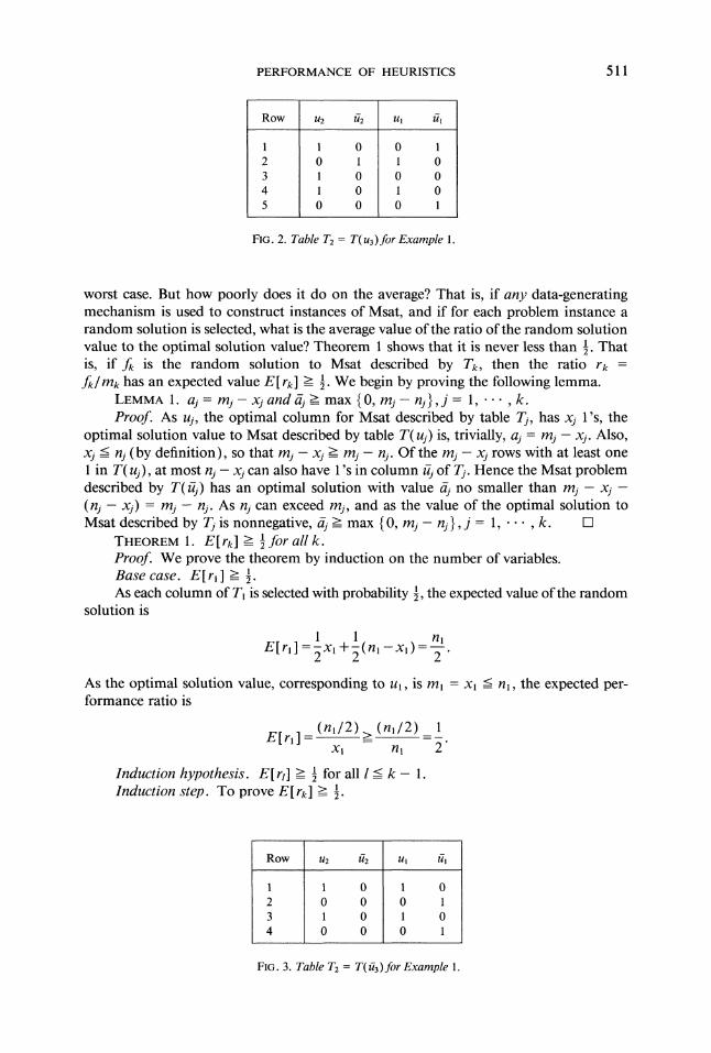
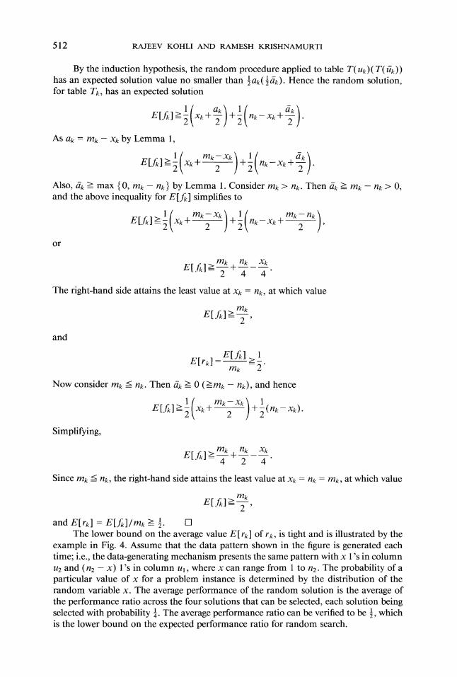
For the table T3 above, table T(u3) is obtained by deleting rows and 4 and thecolumns u3 and if3. Table T2 T(u3) is given in Fig. 2. Similarly, we can obtain tableT(if3) by deleting rows 2, 3, and 5 and the columns u3 and if3. Table T2 T(ff3) is givenin Fig. 3.

Consider a random procedure that selects column u or with probability 1/2, j1, -.., k. The procedure can easily be seen to select an arbitrarily bad solution in the

Row u3 ff

02 03 04 05 06 0 07 0 0

u2 =00

00 0

00

0 0

FIG. 1. Table T3 for Example 1.

PERFORMANCE OF HEURISTICS 51

Row u2 if2

02 03 04 05 0 0

00

o oo

0

FIG. 2. Table T2 T( u3) for Example 1.

worst case. But how poorly does it do on the average? That is, if any data-generatingmechanism is used to construct instances of Msat, and if for each problem instance arandom solution is selected, what is the average value ofthe ratio ofthe random solutionvalue to the optimal solution value? Theorem shows that it is never less than 1/2. Thatis, if J is the random solution to Msat described by Tk, then the ratio rkfk/mk has an expected value E[ rk] >= 1/2. We begin by proving the following lemma.

LEMMA 1. aj mj Xj and 5. >= max { 0, mj nj }, j 1, k.Proof. As uj, the optimal column for Msat described by table T, has xj l’s, the

optimal solution value to Msat described by table T(uj) is, trivially, aj mj xj. Also,xj <= nj (by definition), so that mj xj >= mj nj. Of the mj xj rows with at least onein T(uj), at most nj xj can also have ’s in column z. of T. Hence the Msat problem

described by T() has an optimal solution with value no smaller than mj xj

(nj xj) mj nj. As nj can exceed mj, and as the value of the optimal solution toMsat described by T is nonnegative, >_- max { 0, mj nj }, j 1, k. E]

THEOREM 1. E[ rk] >= 1/2 for all k.Proof. We prove the theorem by induction on the number of variables.Base case. E[ r -> .As each column of Tl is selected with probability 1/2, the expected value ofthe random

solution is

nE[rl]=-Xl +(n -x) =--.

As the optimal solution value, corresponding to u, is ml Xl rt, the expected per-formance ratio is

E[rl] (n/2)>_ (n/2)x n 2"

Induction hypothesis. E[ rt] >= 1/2 for all _-< k 1.Induction step. To prove E[ rk] >= 1/2.

Row U2 /2

02 0 03 04 0 0

0o

o0

FIG. 3. Table T2 T(if3) for Example 1.

512 RAJEEV KOHLI AND RAMESH KRISHNAMURTI

By the induction hypothesis, the random procedure applied to table T( Uk)(T(ffk))has an expected solution value no smaller than 1/2a( 1/2/). Hence the random solution,for table T, has an expected solution

E[JI> x+- + - nk x+-As a m x by Lemma 1,

mk Xk + nk--Xk+E[JI > xk+ 2 -Also, 6 >_- max { 0, m- n } by Lemma 1. Consider m > nk. Then / >_- m- n > 0,and the above inequality for E[J] simplifies to

mk Xk + nk-- Xk +E[A] >_- xk+ 2 E 2

or

mk n_L xE[ Jl >=---t 4 4

The right-hand side attains the least value at x n, at which value

and

E[E[ rk] >_- ".

mk 2

Now consider m _-< n. Then d >= 0 (>mk- n), and hence

1( mk--X)E[A]>- x+ 2 +-(n-x).Simplifying,

mk nk XkE[J] >=--+ 2 -"Since mk <= nk, the fight-hand side attains the least value at x nk mz:, at which value

mkE[j] >

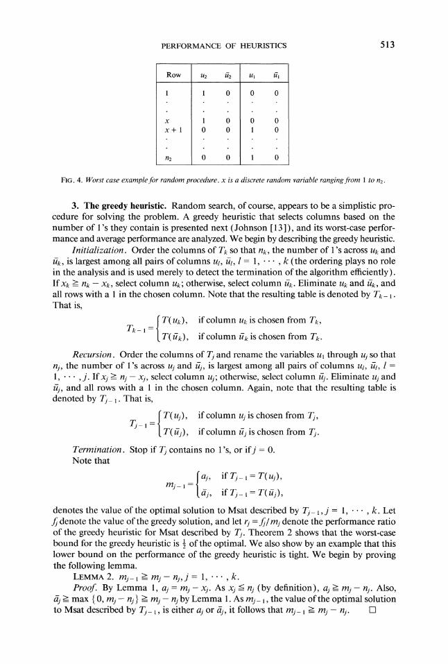
and E[ r] E[f]/mk >= 1/2.The lower bound on the average value E[ r] of r, is tight and is illustrated by the

example in Fig. 4. Assume that the data pattern shown in the figure is generated eachtime; i.e., the data-generating mechanism presents the same pattern with x ’s in columnu2 and (n2 x) ’s in column u,, where x can range from to n2. The probability of aparticular value of x for a problem instance is determined by the distribution of therandom variable x. The average performance of the random solution is the average ofthe performance ratio across the four solutions that can be selected, each solution beingselected with probability . The average performance ratio can be verified to be 1/2, whichis the lower bound on the expected performance ratio for random search.

PERFORMANCE OF HEURISTICS 513

Row u2 2

0

x ox+l 0 0

n2 0 0

ul

0 0

o oo

o

FIG. 4. Worst case examplefor random procedure, x is a discrete random variable rangingfrom to n2.

3. The greedy heuristic. Random search, of course, appears to be a simplistic pro-cedure for solving the problem. A greedy heuristic that selects columns based on thenumber of ’s they contain is presented next (Johnson 13]), and its worst-case perfor-mance and average performance are analyzed. We begin by describing the greedy heuristic.

Initialization. Order the columns of Tk so that nk, the number of ’s across u andu-, is largest among all pairs of columns ut, ill, 1, k (the ordering plays no rolein the analysis and is used merely to detect the termination of the algorithm efficiently).Ifx >= n- x, select column uk; otherwise, select column ff. Eliminate u and ff, andall rows with a in the chosen column. Note that the resulting table is denoted by Tk.- 1.

That is,

if column uk is chosen from T,T_

T(ff), if column ff is chosen from Tk.

Recursion. Order the columns of Tj and rename the variables ul through uj so thatnj, the number of ’s across uj and , is largest among all pairs of columns Ul, ffl,1, j. If xj >= nj xj, select column uj; otherwise, select column . Eliminate uj and, and all rows with a in the chosen column. Again, note that the resulting table isdenoted by Tj_ 1. That is,

T(uj), if column uj is chosen from Tj.,T_

T(/j), if column ffj is chosen from T.Termination. Stop if T contains no ’s, or ifj 0.Note that

aj,

denotes the value of the optimal solution to Msat described by Tj_ l, j 1, k. Letj) denote the value ofthe greedy solution, and let rj fj/mj denote the performance ratioof the greedy heuristic for Msat described by Tj. Theorem 2 shows that the worst-casebound for the greedy heuristic is 1/2 of the optimal. We also show by an example that thislower bound on the performance of the greedy heuristic is tight. We begin by provingthe following lemma.

LEMMA 2. mj_ >= mj- nj, j 1, k.Proof. By Lemma 1, aj mj xj. As xj <= nj (by definition), aj >= mj nj. Also,

> max { 0, mj nj } >= mj nj by Lemma 1. As mj_ l, the value ofthe optimal solutionto Msat described by Tj_ l, is either aj or ., it follows that mj_ - mj rlj. i-1

514 RAJEEV KOHLI AND RAMESH KRISHNAMURTI

THEOREM 2. rk >= 1/2 for all k.Proof. We prove the theorem by induction on the number of variables.Base case. rl > 1/2.The single-variable problem is described by table T1 with column ul containing x

l’s, and column ff containing (n x) l’s. The greedy heuristic selects the columnwith more ’s, which also is the optimal column. Thus

and hence

fl m max { x,, n- xl },

flrl==l>=m 2

Induction hypothesis, rj >= 1/2 for all j < k 1.Induction step. To prove rk >-- 1/2.At the first step, the greedy heuristic chooses uk or ffk, whichever has the larger

number of ’s. Hence

J= max { xk, nk-- Xk } +f-By the induction hypothesis, rk- >_- 1/2, so that

fk- rk- lmk- >=- mk-1.Hence,

A>--max xk, nk-- Xk +- mk-As the maximum of two numbers is no smaller than their mean, max xk, nk xk } >--1/2 nk. Also, by Lemma 2, rnk_ >= mk nk. Thus,

mkfk >=- rlk +- mk- nk) 2"

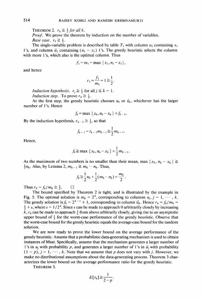
Thus rk f/mk >= 1/2.The bound specified by Theorem 2 is tight, and is illustrated by the example in

Fig. 5. The optimal solution is mk 2 k, corresponding to columns uj, j 1, k.The greedy solution is 2k- + 1, corresponding to column ffk. Hence rk =f/mk1/2 + e, where e /2 k. Since e can be made to approach 0 arbitrarily closely by increasingk, rk can be made to approach 1/2 from above arbitrarily closely, giving rise to an asymptoticupper bound of 1/2 for the worst-case performance of the greedy heuristic. Observe thatthe worst-case bound for the greedy heuristic equals the average-case bound for the randomsolution.

We are now ready to prove the lower bound on the average performance of thegreedy heuristic. Assume that a probabilistic data-generating mechanism is used to obtaininstances of Msat. Specifically, assume that the mechanism generates a larger number of

’s in uj with probability p, and generates a larger number of ’s in G. with probabilityp), j 1, k. Note that we assume that p does not vary with j. However, we

make no distributional assumptions about the data-generating process. Theorem 3 char-acterizes the lower bound on the average performance ratio for the greedy heuristic.

THEOREM 3.

[r]>

PERFORMANCE OF HEURISTICS 515

Row

2k-2

2k-2+

2k-

Uk

0

Uk- k- U2

0 000 0

0 0

0 0

0 0

0 0 0 0

0 0

0 0

0

FIG. 5. Worst case examplefir the greedy heuristic with nk 2 + clauses

Proof. We prove the theorem by induction on the number of variables.Base case. E[ r >= 1/(2 pFor a single-variable problem, the optimal column u has at least as many ’s

as the nonoptimal column ff. Therefore the value of the greedy solution equals thenumber of ’s in the optimal column. Thus, the expected performance ratio ofthe greedyheuristic is

E[f,]E[r] 1_>- for any p, O_-<p_-< 1.

m 2 -p

Induction hypothesis. E[ rt] > /(2 p) for all =< k 1.Induction step. To prove E[rk] > 1/(2 p).If the greedy heuristic selects column uk from T, it guarantees a solution value of

at least x. In addition, table T_ T(u), generated at the first step, describes an Msatproblem for which the expected value ofthe greedy solution is, by the induction hypothesis,no less than [1 /(2 p)]ak. Hence if column u is selected at step 1, the expected valueof the greedy solution is no less than x + /(2 p) a. By a similar argument, if thegreedy heuristic selects ff at step 1, the expected value of its solution is no less thannk x + /(2 p) 7. Now u is selected with probability p, and ff is selected withprobability p). The expected value of the greedy solution is therefore

ak +(l-p) n-x+ 7E[J] >P x+ 2-p 2-p

Noting that ak m x by Lemma 1,

(m-x) +(l-p) nk-x+E[f]>=p x+2_p 2"PAlso, >= max 0, m- nk } by Lemma 1. Consider m > n. Then >- m- nk > 0,

516 RAJEEV KOHLI AND RAMESH KRISHNAMURTI

and the above inequality for E[J] becomes

1-(mk--Xk) +(1 --p) n:--x+E[f] >=p x+-_p 2-p

Simplifying,

1-Pxk+ m +(l-p) n-x+ (m-nk)E[AI>--p2-p 2-p 2-p

Noting that x >_- (n)/2 if column u is chosen and nk x > (nk)/2 if column ff ischosen, we get

m +(l-p) --+ (m-n)2-p 2 2-p 2-p

which implies that

Hence

E[r]E[J] >m 2 -p

Now consider m < nk. Then 7 > 0 (>_-m- n), which implies

Simplifying,

E[J] >p m + -p)2-p 2 2-p

pm+ -p)nkE[j] >=

2-p

As m < n, the fight side of the above expression has a minimum at n m. Hence

pmk + p)rn rnE[J] >= =.2 -p 2 -p

Thus, E[r] (E[f])/m >_- 1/(2 p).The lower bound obtained in Theorem 3 is tight. To illustrate, consider the following

example involving k variables and n 2 rows, where s > k. Generate the data asfollows. Forj 1, k, set

ti,k-j + O, ti,k-j + 1,

ti,k-j + 1, ti,k_ j + O,

li,-j + 1, ti,-j + 0 with probability p,

li,k-j + =O, ti,-j + with probability -p,

if/= 1, ,2 s-J-

ifi=2s-J+ 1, ,2 s-j+l-

if/= 2s-j

if 2-J.

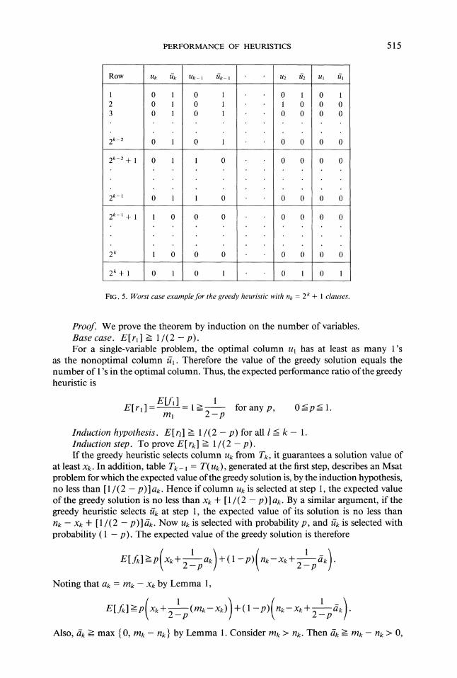
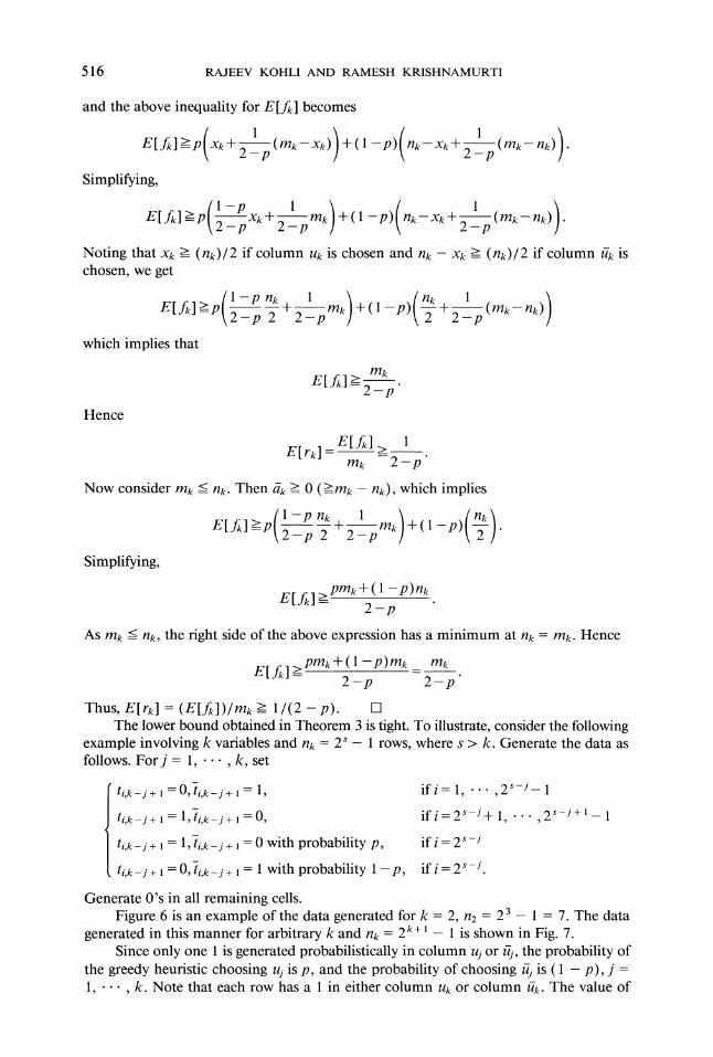
Generate O’s in all remaining cells.Figure 6 is an example of the data generated for k 2, n2 2 7. The data

generated in this manner for arbitrary k and n 2 +l is shown in Fig. 7.Since only one is generated probabilistically in column uj. or z, the probability of

the greedy heuristic choosing u is p, and the probability of choosing z is p), j1, k. Note that each row has a in either column u or column ffk. The value of

PERFORMANCE OF HEURISTICS 517

Row U2 /2

02 03 04 x2 yz5 06 07 0

0Xl Yl

00 00 00 00 0

FIG. 6. Data generatedfor k 2, n2 2 1. xi yi equals 0 with probability p, 0 with probability1-p,fori- 1,2,-..,k.

Row

234

nk+--V--

n,+ 1_4

nk+

nk+l+l4

nk+2

nk+

nk+---+

nk

Uk- k- Uk-2 k-2

000

0000

0

0000

0

Ii

Xk

0

0

xk_

Yk 0

0 0

0 0

FIG. 7. Data generated for arbitrary k and n, 2 k+l 1. xi Yi equals 0 with probability p, 0 withprobability p, for 1, 2, ..., k.

518 RAJEEV KOHLI AND RAMESH KRISHNAMURTI

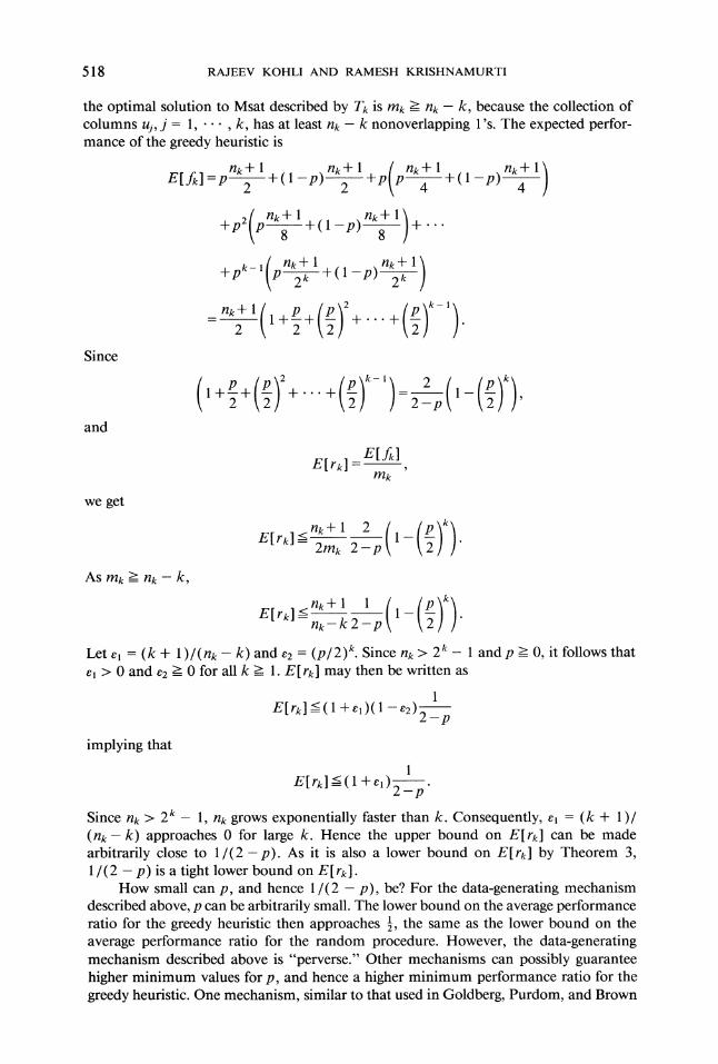
the optimal solution to Msat described by Tk is mk n k, because the collection ofcolumns uj., j 1, k, has at least n k nonoverlapping ’s. The expected perfor-mance of the greedy heuristic is

n,+ n+ ( nk+ n+ 1)E[J]=p2

+(l-p)2

+p p4

+(l-p)4

n+ nk+ 1)k-P2 P 8+(l-p)

8+

( n+l n+l)+pk-1 p.2

+(l-p) 2

2 1+-+ +...+

Since

and

E[r]

we get

n+ 21-E[ rk] <= -m-- 2-p

As m >_- n- k,

n-k 2-p -Let el (k + )/(n k) and e2 (P/2)k. Since ng > 2 and p >_- 0, it follows that

e > 0 and e2 > 0 for all k >_- 1. E[ r] may then be written as

E[r]-< (1 +e,)(1 -e2)2_pimplying that

E[rk] =< +e)2_pSince n > 2 1, n grows exponentially faster than k. Consequently, e (k + )/(n- k) approaches 0 for large k. Hence the upper bound on E[rk] can be madearbitrarily close to 1/(2- p). As it is also a lower bound on E[ rg] by Theorem 3,/(2 p) is a tight lower bound on E[ rg].

How small can p, and hence 1/(2 p), be? For the data-generating mechanismdescribed above, p can be arbitrarily small. The lower bound on the average performanceratio for the greedy heuristic then approaches 1/2, the same as the lower bound on theaverage performance ratio for the random procedure. However, the data-generatingmechanism described above is "perverse." Other mechanisms can possibly guaranteehigher minimum values for p, and hence a higher minimum performance ratio for thegreedy heuristic. One mechanism, similar to that used in Goldberg, Purdom, and Brown

PERFORMANCE OF HEURISTICS 519

], is as follows: for all j 1, k, generate

tij 1,7ij 0, with probability q,

0 0, 7ij 1, with probability q,

o O, ti 0, with probability 2q.

The choice of q is arbitrary, and as in many simulations may be based on randomsampling from a- parametric distribution. In this case, the probability that uj has a largernumber of l’s than is 1/2, j 1, k, and hence E[rk] >- ].

Is there a way to improve the lower bound on E[ rk] for the greedy heuristic? Solong as p is governed by "nature" (i.e., by a data-generating mechanism which the al-gorithm cannot control), there appears to be no way. But there is no reason why thechoice ofp should not be made a part of the heuristic. For instance, we may introduceprobabilistic choice at each step ofthe greedy heuristic so that, whateverp is, the heuristicselects a solution with a probability it chooses. The perversity of a data-generating mech-anism may then be superseded by the heuristic. We pursue this approach below bydescribing a probabilistic version of the greedy heuristic, which we call the probabilisticgreedy heuristic.

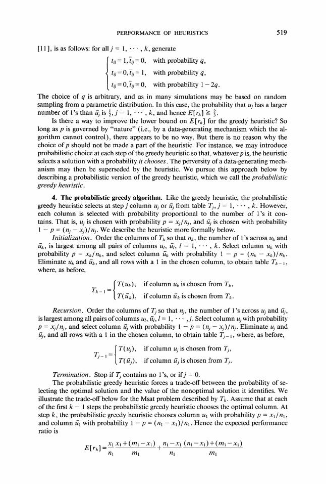
4. The probabilistic greedy algorithm. Like the greedy heuristic, the probabilisticgreedy heuristic selects at step j column uj or zij. from table T, j 1, k. However,each column is selected with probability proportional to the number of l’s it con-tains. That is, u. is chosen with probability p xj/nj, and is chosen with probability

p (nj x9)/n9. We describe the heuristic more formally below.Initialization. Order the columns of T so that n, the number of ’s across ug and

u-, is largest among all pairs of columns ut, fit, 1 1, k. Select column u withprobability p xk/n, and select column ff with probability p (n x)/nk.Eliminate u and ff, and all rows with a in the chosen column, to obtain table T_ ,where, as before,

if column uk is chosen from T,Tk-

T(ffk), if column ffk is chosen from Tk.

Recursion. Order the columns of T so that nj, the number of ’s across u and ff,is largest among all pairs ofcolumns ut, fit, 1, j. Select column uj with probabilityp xj/n, and select column with probability p (n9 xj)/nj. Eliminate uj and, and all rows with a in the chosen column, to obtain table T_ , where, as before,

T(u), if column uj. is chosen from T,Tj_

T(tij.), if column zT is chosen from T.Termination. Stop if T contains no ’s, or ifj 0.The probabilistic greedy heuristic forces a trade-off between the probability of se-

lecting the optimal solution and the value of the nonoptimal solution it identifies. Weillustrate the trade-off below for the Msat problem described by Tk. Assume that at eachof the first k steps the probabilistic greedy heuristic chooses the optimal column. Atstep k, the probabilistic greedy heuristic chooses column u with probability p x/n,and column ff with probability -p (nl x )/n. Hence the expected performanceratio is

E[rk] =xx +(m--x) n--x (n--x)+(m--x)nl ml Hi ml

520 RAJEEV KOHLI AND RAMESH KRISHNAMURTI

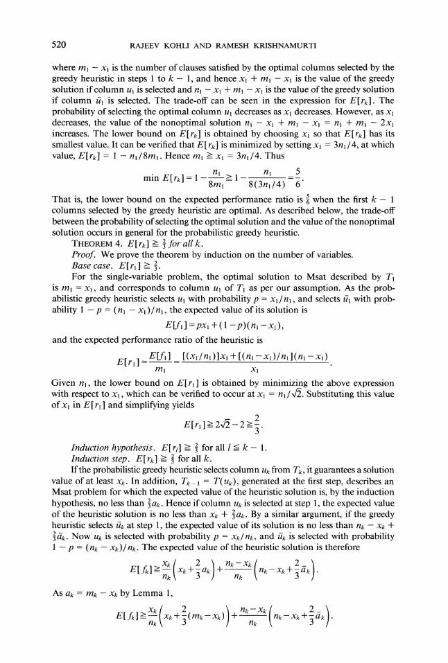
where ml Xl is the number of clauses satisfied by the optimal columns selected by thegreedy heuristic in steps to k l, and hence xl + ml Xl is the value of the greedysolution ifcolumn ul is selected and n x + m x is the value ofthe greedy solutionif column ffl is selected. The trade-off can be seen in the expression for E[rk]. Theprobability of selecting the optimal column u decreases as x decreases. However, as xdecreases, the value of the nonoptimal solution n x + m x n + ml 2xincreases. The lower bound on E[ rk] is obtained by choosing x so that E[ rk] has itssmallest value. It can be verified that E[ rk] is minimized by setting x 3n/4, at whichvalue, E[rk] nl/8m. Hence m -> x 3n/4. Thus

n > 1- n 5min E[rk] 8m---= 8(3n/4) =g"

That is, the lower bound on the expected performance ratio is when the first kcolumns selected by the greedy heuristic are optimal. As described below, the trade-offbetween the probability of selecting the optimal solution and the value ofthe nonoptimalsolution occurs in general for the probabilistic greedy heuristic.

THEOREM 4. E[ rk] >= for all k.Proof. We prove the theorem by induction on the number of variables.Base case. E[ r >= .For the single-variable problem, the optimal solution to Msat described by T1

is ml xl, and corresponds to column u of T as per our assumption. As the prob-abilistic greedy heuristic selects u with probability p x/nl, and selects ff with prob-ability p (nl x )/n, the expected value of its solution is

E[fl] =px +( -p)(n-x),

and the expected performance ratio of the heuristic is

E[f] [(xl/n)]x +[(nl-Xl)/n](n-x)E[rl]

ml Xl

Given n, the lower bound on E[ r] is obtained by minimizing the above expressionwith respect to x, which can be verified to occur at Xl nl/4. Substituting this valueofx in E[ rl] and simplifying yields

2E[r1]>=24-2>_- -.3

Induction hypothesis. E[ r1] > for all _-< k 1.Induction step. E[ rk] >= for all k.Ifthe probabilistic greedy heuristic selects column u from T, it guarantees a solution

value of at least x. In addition, T_ T(uk), generated at the first step, describes anMsat problem for which the expected value of the heuristic solution is, by the inductionhypothesis, no less than a. Hence if column u is selected at step 1, the expected valueof the heuristic solution is no less than x + ga. By a similar argument, if the greedyheuristic selects ffk at step 1, the expected value of its solution is no less than n x +2-ga. Now u is selected with probability p xk/n, and ff is selected with probability

p (n x)/nk. The expected value of the heuristic solution is therefore

= x+ a +... n-x+ dknk - nk -As a =mg xg by Lemma l,

= Xk+ (m--xk) + n--x+n - n -

PERFORMANCE OF HEURISTICS 521

Also, dk >= max 0, mk- n } by Lemma 1. Consider m > n. Then d -> mk- n > 0,and the above inequality for E[J] becomes

Simplifying,

E[f]>x(2m x)-5-+-2 + (n/-- Xk)2 2(n-x)+ m nk).n 3n

E[j]_>(x)2 2mkxk (nk--x) 2 2(n--x)+ + + (m--n).3nk 3n n 3n

The fight side of the above expression can be verified to obtain its minimum value whenx nk/2, at which value of x,

2m[A]>3

and hence

E[J] 2E[r] >=-.

m 3

Now consider mk -< nk. Then d >= 0 (>m n), and hence

Simplifying

E[j]>xk( 2 ) n--x= xk+ (m--Xk) + (n--x).flk nk

2mx (nk-- Xk) 2

[A] > (x)- + +3n 3n n

The fight side of the above expression can be verified to obtain its minimum value whenx (3n mk)/4, at which value ofx

nk mk mE[J] >=---+ 2 12n"The fight side of the above expression takes its smallest value when n m, for which

mk m m 2E[J] >-----+- 1-- m.

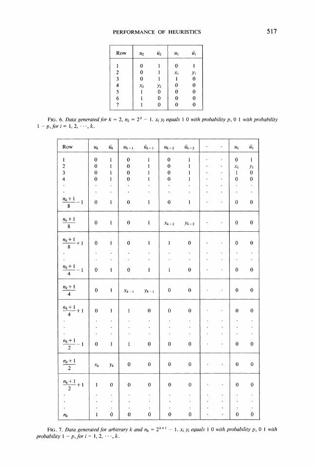
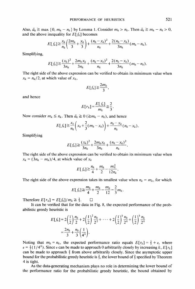
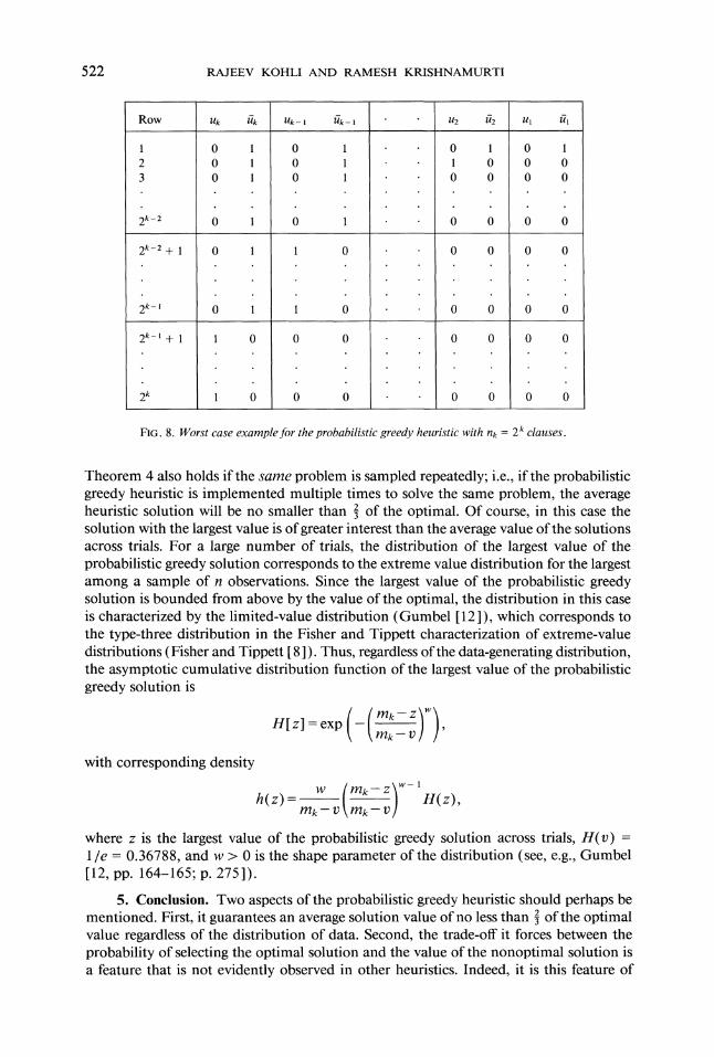
Therefore E[r] E[f]/m >= .It can be verified that for the data in Fig. 8, the expected performance of the prob-

abilistic greedy heuristic is

el= + +.+ +3 +T

Noting that m n, the expected performance ratio equals E[r] + e, wheree / 4). Since e can be made to approach 0 arbitrarily closely by increasing k, E[ rcan be made to approach from above arbitrarily closely. Since the asymptotic upperbound for the probabilistic eedy heuristic is , the lower bound of specified by Theorem4 is tight.

As the data-generating mechanism plays no role in determining the lower bound ofthe performance ratio for the probabilistic greedy heuristic, the bound obtained by

522 RAJEEV KOHLI AND RAMESH KRISHNAMURTI

Row

2k-2

2k-2+

2k-

2k-+

2

000

0

Uk-I k-I

000

0

0 0

U2 2

00

0 0

0 0

FIG. 8. Worst case examplefor the probabilistic greedy heuristic with n 2 clauses.

Theorem 4 also holds if the same problem is sampled repeatedly; i.e., if the probabilisticgreedy heuristic is implemented multiple times to solve the same problem, the averageheuristic solution will be no smaller than of the optimal. Of course, in this case thesolution with the largest value is ofgreater interest than the average value ofthe solutionsacross trials. For a large number of trials, the distribution of the largest value of theprobabilistic greedy solution corresponds to the extreme value distribution for the largestamong a sample of n observations. Since the largest value of the probabilistic greedysolution is bounded from above by the value of the optimal, the distribution in this caseis characterized by the limited-value distribution (Gumbel [12 ), which corresponds tothe type-three distribution in the Fisher and Tippett characterization of extreme-valuedistributions (Fisher and Tippett 8 ]). Thus, regardless ofthe data-generating distribution,the asymptotic cumulative distribution function of the largest value of the probabilisticgreedy solution is

H[z] =exp

with corresponding density

W(mk--Z)w-1

H(z),h(z)mk--V mk--v

where z is the largest value of the probabilistic greedy solution across trials, H(v)1/e 0.36788, and w > 0 is the shape parameter of the distribution (see, e.g., Gumbel[12, pp. 164-165; p. 275]).

5. Conclusion. Two aspects of the probabilistic greedy heuristic should perhaps bementioned. First, it guarantees an average solution value ofno less than ofthe optimalvalue regardless of the distribution of data. Second, the trade-off it forces between theprobability of selecting the optimal solution and the value of the nonoptimal solution isa feature that is not evidently observed in other heuristics. Indeed, it is this feature of

PERFORMANCE OF HEURISTICS 523

the heuristic that ensures that its average performance is never too bad. In contrast, whilethe greedy heuristic can do well, its ability to do so depends on the value of p. Forindependent observations from parametric distributions with p 1/2, it does as well, onaverage, as the probabilistic greedy heuristic. But for perverse distributions, the greedyheuristic on average can do as poorly as random search. On the other hand, for an"unintelligent" procedure, the random search does quite well to ensure an average solutionof no less than 1/2 of the optimal, regardless of the data-generating distribution. It remainsan open question whether relaxing the independence assumption, or assuming specificdistributions, strengthens the bounds on the average performance for the greedy heuristic.It may also be possible to strengthen the average bound for the greedy heuristic withrestricting assumptions on problem instances, such as when the set of clauses are 2-satisfiable (Lieberherr and Specker 16 ), or when each clause contains at least variables,

-< =< k (Johnson [13]).

Acknowledgments. The authors thank Pavol Hell, Tiko Kameda, Art Liestman,Joe Peters, and Art Warburton for numerous helpful suggestions. Special thanks are dueto Tiko Kameda and Joe Peters for carefully reading the paper and giving detailed com-ments that have helped improve the presentation.

REFERENCES

J. BENTLEY, D. S. JOHNSON, F. T. LEIGHTON, AND L. A. MCGEOCH, Some unexpected expected behaviorresultsfor bin packing, Proc. 16th ACM Sympos. Theory of Computing, 1984, pp. 279-288.

2 O. J. BOXMA, A probabilistic analysis ofmultiprocessing list scheduling: the erlang case, Stochastic Models,(1985), pp. 209-220.

3 J. L. BRUNO aND P. J. DOWNEY, Probabilistic boundsfor dual bin packing, Acta Inform., 22 (1985), pp.333-345.

4 E.G. COMaN aND F. T. LEIGHTON, A provably efficient algorithmfor dynamic storage allocation, Proc.18th ACM Sympos. Theory of Computing, 1986, pp. 77-90.

5 E. G. COFFMAN, G. S. LUEKER, AND A. H. G. RINNOOY KAY, Asymptotic methods in the probabilisticanalysis ofsequencing and packing heuristics, Management Sci., 3 1988 ), pp. 266-290.

[6] J. CSIRIK, J. B. G. FRENK, A. FRIEZE, G. GALAMBOS, AND A. H. G. RINNOOY KAN, A probabilisticanalysis ofthe next fit decreasing bin packing heuristic, Oper. Res. Lett., 5 (1986), pp. 233-236.

7 M. Davis, G. LOGEMANN, AND D. LOVELAND, A machine programfor theorem proving, Comm. ACM,5 (1962), pp. 394-397.

8 R. A. FISHER AND L. H. C. TIPPETT, Limitingforms ofthefrequency distribution ofthe largest or smallestmember ofa sample, Proc. Cambridge Phil. Soc., 24 (1928), pp. 180-190.

9 J. FRANCO AND M. PAULL, Probabilistic analysis ofthe Davis Putnam procedurefor solving the satisfiabilityproblem, Discrete Applied Math., 5 (1983), pp. 77-87.

10 J. B. G. FRENK AND A. H. G. RINNOOY KAN, The asymptotic optimality ofthe LPT rule, Math. Oper.Res., 12 (1987), pp. 241-254.

11 A. GOLDBERG, P. PURDOM, AND C. BROWN, Average time analysis ofsimplified Davis-Putnam procedures,Inform. Process. Lett., 15 (1982), pp. 72-75.

12] E. J. GUMBEL, Statistics ofExtremes, Columbia University Press, New York, 1958.13 D. S. JOHNSON, Approximation algorithmsfor combinatorialproblems, J. Comput. System Sci., 9 (1974),

pp. 256-278.14] R. M. KARP, M. LUBY, AND A. MARCHETTI-SPACCAMELA, A probabilistic analysis ofmultidimensional

bin packing problems, Proc. 16th ACM Sympos. Theory of Computing, 1984, pp. 289-298.15 F. T. LEIGHTON AND P. W. SHOR, Tight bounds for minimax grid matching with applications to the

average-case analysis ofalgorithms, Proc. 18th ACM Sympos. Theory of Computing, 1986, pp. 91-103.

[16] K. J. LIEBERHERR AND E. SPECKER, Complexity ofpartial satisfaction, J. Assoc. Comput. Mach., 281981 ), pp. 411-421.

[17] P. W. SHOR, The average-case analysis of some on-line algorithms for bin packing, Combinatorica, 6(1986), pp. 179-200.