Performance Measures

This note provides a detailed description of the measures used in this study to quantitatively and

objectively evaluate the performance of the particle tracking methods.

INTRODUCTION

The problem of performance evaluation of tracking methods occurs in many fields, including computer

vision, aerospace applications (radar tracking, navigation, traffic control), and biomedical research.

Despite much consideration in the past decades,1-3 there is as yet no single, well-accepted method to

evaluate overall tracking performance. This can be explained by the fact that different application areas

may be concerned with different aspects of track estimation and, consequently, may require different

performance measures. In particular, measures proposed in other fields are often not applicable to

biological particle tracking, where one is faced with a priori unknown and varying numbers of particles,

whose identities are to be preserved throughout the image sequence.4,5

A key aspect of comparing a set of estimated objects to a set of known but possibly a different number

of ground-truth objects, is the pairing of their elements: which element in the former should be

compared to which element in the latter? A sensible approach to solving this problem for sets of

positions is the use of optimal subpattern assignment.6,7 This concept has recently also been extended to

sets of labeled object tracks.8 The evaluation of particle tracking methods in the present study was based

on the same underlying idea, as described in detail below. Nevertheless, in order to have a complete and

intuitive characterization of the performance of the different methods, a set of complementary

performance measures was used, rather than a single measure.

TRACK DEFINITION

A track is a temporal series of subsequent spatial positions. The spatial position at a given time point

is a vector , with , , and the coordinates at this time along

the respective axes of the image. In a 3D image sequence, all three coordinates may vary, while in a 2D

image sequence, the coordinate is fixed. A track existing from time to time is

therefore defined as the set . Missing positions in the interval are

marked as non-matching and are penalized as described below.

DISTANCE BETWEEN TWO TRACKS

For the purpose of measuring the distance between two tracks, the following gated Euclidean distance

between two positions and is defined:

with the standard norm of , and the gate. The rationale behind the use of the gate is

to limit the penalization of tracks that separate. When two tracks are more than apart at any time , it

is indeed considered that their positions do not match at that time point. In that case, it is irrelevant to

measure the actual distance between these positions, and a fixed penalty is used instead. In the

context of this study, the value of was set to 5 pixels, which, for the imaging parameters simulated in

our data, was on the order of the Rayleigh criterion.9,10 In other words, the required minimum distance

between diffraction-limited particles to allow visual separation (Rayleigh), was taken as the maximum

tolerable distance for the particle tracking methods.

It may happen that two tracks have different temporal supports. For instance, may exist at a given

time , while does not. In that case, we consider that the tracks do not match at that time point, and

the distance between the tracks is defined to be equal to the penalty . If neither of the two tracks exist

at time , their distance is defined to be 0. This allows for the following compact formulation of the

distance between any two tracks and :

where is the length (the number of frames) of the image sequence.

DISTANCE BETWEEN TWO TRACK SETS

Let be an ordered set of ground-truth tracks, and a set of estimated tracks,

whose similarity to needs to be evaluated. Since some tracks in may not match a track in , or vice

versa, is extended with dummy tracks that are empty. Let denote this extended set of estimated

tracks. Furthermore, let be the ensemble of ordered sets of tracks that can be obtained by taking

elements from . The distance between any and is then defined as the sum of the distances

between the pairs of tracks given by the ordering of the two sets. This allows for the definition of the

distance between and as the minimum distance between and all possible :

Building the set of tracks that minimizes the distance to , involves reordering and taking a

subset of elements from it. This task can be viewed as a rectangular assignment problem between

the tracks in and . Because of the additivity and positivity of the cost of track association according to

the above definition, this problem can be solved in polynomial time, using the Munkres algorithm.11

PERFORMANCE MEASURES

In order to evaluate the performance of any particle tracking method for any data, the output track set

of the method was scored with respect to the ground-truth track set of that data using the following

measures, based on the optimal pairing described above:

1) The measure , where denotes the set of dummy tracks. By

definition of , the lower bound of is 0, and the upper bound is . Indeed, a pair

of tracks

is guaranteed not to be selected by the optimization process if the distance

between them is larger than the distance between and a dummy track. The value of measure

therefore lies in the interval . It takes value 1 if the pairs of tracks in and match

exactly (the distance between each pair of tracks is 0). It takes value 0 if no valid match could be

found, that is if . It scores the best possible pairing of tracks between and , and ignores

the tracks in that did not make it into .

2) The measure , where denotes

the set of tracks in that did not make it into , and contains the appropriate number of dummy

tracks, being for and for . A track in may not have been selected for

because either another estimated track or a dummy track was preferred over it. Such a spurious

track typically consists of a combination of positions corresponding to different ground-truth tracks

or to erroneous positions originating from clutter. The value of lies in . It takes

value if there are no spurious tracks in , that is if . And it converges to 0 as the

number of spurious tracks increases.

The measures and account for both association errors and localization errors. For a more detailed

analysis, it is useful to separate these two types of errors. To evaluate association performance, the

positions at time of two paired tracks, and

, are counted as matching if they are both non-

dummy and

. Otherwise, they are counted as non-matching, with the exception

of two dummy positions, which are not counted. This leads to the following measures:

3) The number of matching positions of the optimal pairs of tracks . These are referred to as true

positive ( ) position pairs.

4) The number of positions in that are paired with a dummy position in . These are referred to as

false negative ( ) position pairs because the dummy positions are nevertheless associated with

track positions in the ground-truth set .

5) The number of positions in the spurious tracks and the non-matching positions in . These are

referred to as false positive ( ) positions because they correspond to estimated positions that were

not associated with track positions in the ground-truth set .

6) The Jaccard similarity coefficient12 for positions, defined as , which lies in

the interval . It takes value 1 only if all position pairs in are matching and . It

converges to 0 as the number of non-matching pairs and/or positions in increases.

It may also be useful to evaluate the association performance at the track level, rather than the position

level. This leads to the following measures, analogous to the previous four measures:

7) The number of non-dummy tracks in . They are referred to as true positive tracks ( ) because

each of them contains a majority of matching positions with a single associated track in .

8) The number of dummy tracks in . These are referred to as false negative tracks ( ) because

each of them is nevertheless associated with a single track in .

9) The number of tracks in . These are referred to as false positive tracks ( ) because none of them

is associated with a track in .

10) The Jaccard similarity coefficient for tracks, defined as , which lies

in the interval . It takes value 1 only if does not contain dummy tracks and . It

converges to 0 as the number of dummy tracks in and/or tracks in increases.

Finally, the localization performance is characterized by the Euclidean distance (referred to as the error)

between the positions of paired tracks. Since non-matching positions are already penalized by the above

measures, the computation of localization errors is limited to matching positions:

11) The root mean-square error ( ) in true positive position pairs ( as above).

12) The minimum error ( ) in position pairs.

13) The maximum error ( ) in position pairs.

14) The standard deviation ( ) of error in position pairs.

EXAMPLE CASES AND PERFORMANCE VALUES

To illustrate the effect of various tracking errors on the different performance measures, we provide

several synthetic examples of increasing complexity. In the examples, a track is graphically represented

as a series of point markers whose centers indicate the spatial position of the underlying particle at

different time points, which are projected into a single image (Figure N1). The progression through time

is indicated by a line connecting the point markers of the track. Tracks from the ground-truth set are

indicated by square-shaped markers connected by solid lines, while tracks from the estimated set are

indicated by cross-shaped markers connected by dotted lines.

Figure N1: Ground-truth track defined for five successive time points ( ). In the

sequel we will omit the time labels from the point markers and consider the left-most

marker as the starting point of the track.

CASE 1: NO ESTIMATED TRACKS

We start with the pathological case in which we have a single particle with ground truth ( as given in

Figure N1) and the particle tracking method could not find any part of the track ( ). In this case, by

definition, . Also, since there are no estimated tracks at all, we have , and

instead a dummy track is paired with the ground-truth track, yielding , leading to .

Similarly, we have , and since the ground-truth track covers five time points, we have the

same number of matching dummy positions, , yielding . Without any positions it is not

possible to assess the localization performance of the tracking method.

CASE 2: ESTIMATED TRACKS IDENTICAL TO GROUND-TRUTH TRACKS

The other extreme is the case where the output of the particle tracking method is identical to the ground

truth ( as in Figure N2). In this case, the number of matching tracks in is exactly the number of

elements in , here , and since there are no dummy or spurious tracks, we have

, and thus . Similarly, the number of positions in is exactly the number of positions in , here

, and , yielding . Because the distance between each pair of estimated and

ground-truth positions is , we have , and all localization errors are .

Figure N2: Ground-truth track (square-shaped markers connected by a solid line) with a

perfectly matching estimated track (cross-shaped markers connected by a dotted line that

is fully overlapping and thus not visible). The larger, light colored circles around the ground-

truth positions indicate the gate within which estimated positions are searched.

CASE 3: FULLY MATCHING BUT NOT IDENTICAL TRACKS

In this example, we consider a similar situation as in Case 2, where an optimal pairing of estimated and

ground-truth tracks is possible without the need for dummy tracks and without leaving spurious tracks,

but where the estimated positions are not identical to the ground-truth positions, although they are

within the gates of the latter (Figure N3). The distortions in the estimated positions affect only and

and the localization measures. Since there are no spurious tracks, , and in this example both drop

to . The localization errors all become (we refer to Table N1 at the end of this section for the

values of the performance measures for all example cases discussed).

Figure N3: Ground-truth track (squares connected by solid lines) with a paired estimated

track (crosses connected by dotted lines) whose positions are not identical with, but fall

within, the gates (light colored circles) of the ground-truth positions.

CASE 4: MATCHING TRACKS HAVING NON-MATCHING POSITIONS

Next, we reconsider the situation of Case 3, and move one of the estimated track positions out of the

gate of the corresponding ground-truth track position (Figure N4).

Figure N4: Estimated track (crosses connected by dotted lines) that is paired with a ground-

truth track (squares connected by solid lines) but with one position (underscored cross)

falling outside the gate of the ground-truth track position (underscored square).

As a result, this estimated position is considered non-matching with the ground truth, which translates

into an increase in the number of false-positive positions, . At the same time, the ground-truth

position is now matched with a dummy position, leading to , and since , we have

. The dummy position receives a penalty that is larger than the localization error of the

original position in Case 3, leading to a decrease of both and . Also, the computation of , which

is limited to positions only, no longer includes the now non-matching position, whose localization

error was relatively large, and as a result slightly decreases while slightly increases. All other

performance measures remain unaffected by the change (Table N1).

CASE 5: MATCHING TRACKS WITH BIRTH AND DEATH MISMATCHES

In the previous examples we compared tracks (estimated versus ground truth) that were defined over

the same time interval. Now we consider a case in which the existence window of the estimated track is

shifted by one time point compared to the ground-truth track (Figure N5). This is representative of cases

where a particle tracking method fails to detect the right birth and death times of a particle.

Figure N5: Estimated track (crosses connected by dotted lines) that is paired with a ground-

truth track (squares connected by solid lines) but whose start and end positions do not

correspond to the ground truth (all problematic positions are underscored).

Since the majority of the track positions still match, the two tracks are paired by the track association

algorithm, and similar to Case 4 only the performance measures accounting for position matching and

localization errors are affected (Table N1). Specifically, since further decreases to , and increases

to , and the number of matched dummy positions also increases to 2, drops to , and both

and significantly drop to . Because we are now missing one more position (the left-most) with

a relatively large localization error, again slightly decreases and slightly increases.

CASE 6: MULTIPLE ESTIMATED AND GROUND-TRUTH TRACKS

In the following examples (Cases 6-10) we consider multiple estimated and ground-truth tracks. Together

they cover all the types of situations encountered in our study. As a first example we extend Case 5 with

one additional estimated and corresponding ground-truth track (Figure N6).

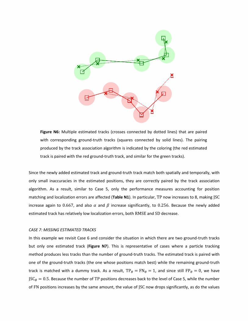
Figure N6: Multiple estimated tracks (crosses connected by dotted lines) that are paired

with corresponding ground-truth tracks (squares connected by solid lines). The pairing

produced by the track association algorithm is indicated by the coloring (the red estimated

track is paired with the red ground-truth track, and similar for the green tracks).

Since the newly added estimated track and ground-truth track match both spatially and temporally, with

only small inaccuracies in the estimated positions, they are correctly paired by the track association

algorithm. As a result, similar to Case 5, only the performance measures accounting for position

matching and localization errors are affected (Table N1). In particular, now increases to 8, making

increase again to , and also and increase significantly, to . Because the newly added

estimated track has relatively low localization errors, both and decrease.

CASE 7: MISSING ESTIMATED TRACKS

In this example we revisit Case 6 and consider the situation in which there are two ground-truth tracks

but only one estimated track (Figure N7). This is representative of cases where a particle tracking

method produces less tracks than the number of ground-truth tracks. The estimated track is paired with

one of the ground-truth tracks (the one whose positions match best) while the remaining ground-truth

track is matched with a dummy track. As a result, , and since still , we have

. Because the number of positions decreases back to the level of Case 5, while the number

of positions increases by the same amount, the value of now drops significantly, as do the values

of both and (Table N1). And since localization errors are computed only for positions, the values

of the corresponding performance measures are the same as in Case 5.

Figure N7: Two ground-truth tracks (squares connected by solid lines) but only one

estimated track (crosses connected by dotted lines). The pairing produced by the track

association algorithm is indicated by the coloring (the red estimated track is paired with the

red ground-truth track while the green ground-truth track is paired with a dummy).

CASE 8: SPURIOUS ESTIMATED TRACKS

Here we again revisit Case 6, but consider the reverse situation as in Case 7, in that we now have two

estimated tracks but only one ground-truth track (Figure N8). This is representative of cases where a

particle tracking method produces more tracks than the number of ground-truth tracks. One of the

estimated tracks (whose positions match best) is paired with the single ground-truth track while the

other estimated track is considered spurious and remains non-paired. As a result, , and

since , we still have . Because the and positions are interchanged compared to

Case 7, the value of remains the same, but increases back to the level of Case 5 (Table N1), as it

does not penalize spurious tracks. And since localization errors are computed only for positions, the

values of the corresponding performance measures are the same as in Cases 5 and 7.

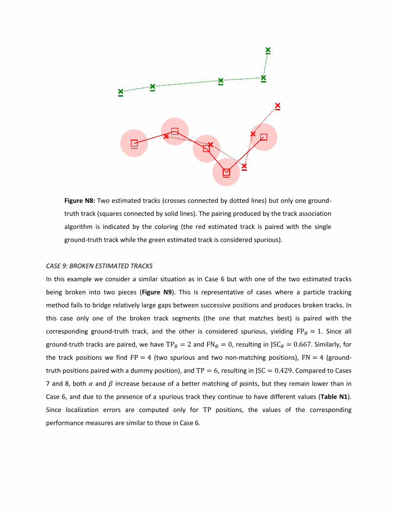
Figure N8: Two estimated tracks (crosses connected by dotted lines) but only one ground-

truth track (squares connected by solid lines). The pairing produced by the track association

algorithm is indicated by the coloring (the red estimated track is paired with the single

ground-truth track while the green estimated track is considered spurious).

CASE 9: BROKEN ESTIMATED TRACKS

In this example we consider a similar situation as in Case 6 but with one of the two estimated tracks

being broken into two pieces (Figure N9). This is representative of cases where a particle tracking

method fails to bridge relatively large gaps between successive positions and produces broken tracks. In

this case only one of the broken track segments (the one that matches best) is paired with the

corresponding ground-truth track, and the other is considered spurious, yielding . Since all

ground-truth tracks are paired, we have and , resulting in . Similarly, for

the track positions we find (two spurious and two non-matching positions), (ground-

truth positions paired with a dummy position), and , resulting in . Compared to Cases

7 and 8, both and increase because of a better matching of points, but they remain lower than in

Case 6, and due to the presence of a spurious track they continue to have different values (Table N1).

Since localization errors are computed only for positions, the values of the corresponding

performance measures are similar to those in Case 6.

Figure N9: Two ground-truth tracks (squares connected by solid lines) but three estimated

tracks (crosses connected by dotted lines) resulting from a linking failure. The pairing

produced by the track association algorithm is indicated by the coloring (the red estimated

track is paired with the red ground-truth track, and the green estimated track is paired with

the green ground-truth track, while the black estimated track is considered spurious).

CASE 10: MIXED UP ESTIMATED TRACKS

In this last example we revisit Case 9 and consider estimated tracks consisting of detected particle

positions belonging to different ground-truth tracks (Figure N10). This is representative of cases where a

particle tracking method erroneously switches particle tracks. In the particular case considered here, one

estimated track is paired with one of the ground-truth tracks, thus , but the other estimated

track does not match with the other ground-truth track, as the majority of its positions is too far off. It

thus remains non-paired, yielding , and consequently the ground-truth track is paired with a

dummy track, yielding , and thus . In terms of positions we find that ,

while , resulting in . Both and decrease compared to Case 9 (Table N1) while

remaining different from each other due to the presence of a spurious track. Finally, the localization

errors are now computed based on only three positions, and are relatively small.

Figure N10: Two ground-truth tracks (squares connected by solid lines) and two estimated

tracks (crosses connected by dotted lines) resulting from linking failures. The pairing

produced by the track association algorithm is indicated by the coloring (the green

estimated track is paired with the green ground-truth track while the black estimated track

is not paired but considered spurious).

Table N1: Overview of the performance values for all discussed example cases. All floating-

point values are given with three decimal places.

Case

1 0.000 0.000 0 5 0 0.000 0 1 0 0.000 - - - -

2 1.000 1.000 5 0 0 1.000 1 0 0 1.000 0.000 0.000 0.000 0.000

3 0.364 0.364 5 0 0 1.000 1 0 0 1.000 3.317 1.414 4.123 0.935

4 0.308 0.308 4 1 1 0.667 1 0 0 1.000 3.240 1.414 4.123 1.018

5 0.052 0.052 3 2 2 0.429 1 0 0 1.000 3.109 1.414 4.123 1.121

6 0.256 0.256 8 2 2 0.667 2 0 0 1.000 2.894 1.414 4.123 0.822

7 0.026 0.026 3 7 2 0.250 1 1 0 0.500 3.109 1.414 4.123 1.121

8 0.052 0.026 3 2 7 0.250 1 0 1 0.500 3.109 1.414 4.123 1.121

9 0.168 0.140 6 4 4 0.429 2 0 1 0.667 2.887 1.414 4.123 0.828

10 0.142 0.089 3 7 7 0.176 1 1 1 0.333 2.646 2.236 2.828 0.279

REFERENCES

1. Fridling BE, Drummond OE. Performance evaluation methods for multiple-target-tracking algorithms.

Proceedings of SPIE: Signal and Data Processing of Small Targets 1481, 371–383 (1991).

2. Blackman S, Popoli R. Design and Analysis of Modern Tracking Systems. Artech House, Norwood, MA,

USA (1999).

3. Rothrock RL, Drummond OE. Performance metrics for multiple-sensor, multiple-target tracking.

Proceedings of SPIE: Signal and Data Processing of Small Targets 4048, 521–531 (2000).

4. Meijering E, Smal I, Danuser G. Tracking in molecular bioimaging. IEEE Signal Processing Magazine

23, 46-53 (2006).

5. Meijering E, Dzyubachyk O, Smal I, van Cappellen WA. Tracking in cell and developmental biology.

Seminars in Cell and Developmental Biology 20, 894-902 (2009).

6. Hoffman JR, Mahler RPS. Multitarget miss distance via optimal assignment. IEEE Transactions on

Systems, Man, and Cybernetics - Part A: Systems and Humans 34, 327-336 (2004).

7. Schuhmacher D, Vo B-T, Vo B-N. A consistent metric for performance evaluation of multi-object

filters. IEEE Transactions on Signal Processing 56, 3447-3457 (2008).

8. Ristic B, Vo B-N, Clark D, Vo B-T. A metric for performance evaluation of multi-target tracking

algorithms. IEEE Transactions on Signal Processing 59, 3452-3457 (2011).

9. Born M, Wolf E. Principles of Optics: Electromagnetic Theory of Propagation, Interference and

Diffraction of Light. 7th Edition. Cambridge University Press, Cambridge, UK (1999).

10. Ram S, Ward ES, Ober RJ. Beyond Rayleigh's criterion: A resolution measure with application to

single-molecule microscopy. Proceedings of the National Academy of Sciences of the United States of

America 103, 4457-4462 (2006).

11. Munkres J. Algorithms for the assignment and transportation problems. Journal of the Society for

Industrial and Applied Mathematics 5, 32–38 (1957).

12. Tan P-N, Steinbach M, Kumar V. Introduction to Data Mining. Addison Wesley, Boston, MA, USA

(2005).