Tech nical Report654

Performance of Bayes-Optimal

Angle -of-Arrival Estimators

F.M. White

13 August 1984

Lincoln Laboratory

Pri-part-A for the Depairiment of Defebnt

tind r £H-s-troriie S~vsemy Disi-.on Conlr., t F19628.8o.(:41002.

OCT I 1984x~p#rb ~rd for publie reIva4e; distr.Ljalion tiniwmitedu.

84 10 11 00f

MASSACHUSETTS INSTITUTE OF TECHNOLOGYLINCOLN LABORATORY

PERFORMANCE OF BAYES-OPTIMALANGLE-OF-ARIVAL ESTIMATORS

F.M. WHITE

Group 44

TECHNICAL REPORT 654

13 AUGUST 1984

Approved for public release distribution unlimited.

LEXINGTON MASSACHUSETTS

% . ,° - .- . .

ABSTRACT

'The angle-of-arrival estimation problem for waves incident upon a sensor

array was examined through a Monte Carlo evaluation of the performance of the

Bayes-optimal MAP (maximum aposteriori) and MHSE (minimum mean square error)

estimators. The case of two independent wave emitters of known powers as well

as a multiple look, Gaussian signal in Gaussian noise statistical model were

a, assumed. The Cramer-Rao bound on the estimator's rms error was computed for

.."' comparison.

The evaluation proceeded with the computation of MAP and ?MSE angle esti-

mates for 1000 random samples of array outputs and the accumulation of theirrms errors. The probability of detecting both emitters with the optimal de-

tector was also accumulated. This was done for .1, .03, and .01 beawrldths

emitter separations and a range of signal-to-noise ratios (SNRs). The ac-

curacy of the computations was assured through a simple finite grid approxima-

tion for the estimates, with no convergence problem, and through the evalua-

tion of statistical confidence intervals for the-Monte Carlo data.

Tie results of the evaluation indicated that the Crauer-Rao bound was

achievable by both the MAP and ?MSE estimators over a wide range of SNR pro-

vided a few as 10 looks had been taken. In general, the bound was achieved

wherever both signals were detectable. These results were surprising since

the bound exhibited unusual behavior; for example, in one SNR region, the

bound showed smaller rms errors for more closely-spaced emitters.

Additional results included properties of the aposteriori probability

density and an analytical computation of the performance of the known angles-

of-arrival optimal detector.

, Accession For5'.4 *I NTIS GRA&I

.5 DTIC TABUnannouncedJustification

ByDistribution/

Availability Codes

Avail and/orDist Lpecial5J" iii

CONTENTS

Abstract III

1.0. INTRODUCTION 1

1.1. AOA Estimation with Sensor Arrays 1

1.2. Statistical Model 5

1.3. Cramer-Rao Bound 91.4. Optimal Estimation and Detection 14

1.4.1. Estimation 141.4.2. Detection 17

1.5. Previous Work - Present Contribution 18

2.0. THE MAP AND MMSE ESTIMATORS AND THE OPTIMAL DETECTOR 20

2.1. MAP and MMSE Estimators 20

2.2. Optimal Detector 22

2.3. Examples of Properties of p( _R) 24

3.0. MONTE CARLO PERFORMANCE EVALUATION 31

3.1. Computational Procedure 31

3.1.1. RMS Error Calculation 31

3.1.2. Probability of Detection Computation 35

3.1.3. Bias Computation 37

3.2. Results 37

3.2.1. RMS Error Results 38

3.2.2. Probability of Detection Results 41

3.2.3. Bias Results 47

4.0. CONCLUSIONS AND RECOMMENDATIONS FOR FURTHER RESEARCH 51ACKNOWLEDGEMENTS 53

REFERENCES 54

APPENDIX A - CONFIDENCE INTERVALS FOR THE MONTE CARLO RESULTS 57

APPENDIX B - THE KNOWN ANGLE-OF-ARRIVAL DETECTOR 61

v

1.0 INTRODUCTION

The estimation of the angles-of-arrival of wavefronts incident upon a

sensor array is a well-known and important problem, occuring in such varied

fields as geophysics, oceanography, emitter location, etc. For small angular

separations of the waves or for small array apertures, estimation is

difficult. As more and more performance is desired of such estimators, as the

cost of physically large sensor arrays increases, and as the cost of real-time

digital computation drops, the possibility of statistically optimum estimation

becomes increasingly interesting and practical.

The goal of this report is not to develop a practical optimal estimator

but rather to compute the performance of the optimal estimators and compare

this performance to the Cramer-Rao bound. More specifically, assuming a

Caussian signal model with two incident waves of known powers, the rms error

of the Bayes-optimal HAP (maximum aposteriori) and MHSE (minimum mean square

error) estimators will be compared via a Monte Carlo simulation, and compared

to the known powers Cramer-Rao bound. These rms errors will provide an

absolute lower bound on the attainable rms error in angle-of-arrival esimation

and will determine the tightness of the Cramer-Rao bound for this problem.

1.1 AOA Estimation with Sensor Arrays

The angle-of-arrival (AOA) estimation problem in its most general form

consists of the estimation of the wavevectors kj of say D incident waves

based on the outputs of N arbitrarily placed wavefield sensors. Each sensor

output is some known function of the field in its vicinity.

In this report, we specialize the problem to a simpler though common

case. Later, we assume only two waves (D-2) in order to make computations

feasible, but will keep D arbitrary whenever possible. Assume that all of the

T waves are monochromatic plane waves with wave-vectors kj, complex

amplitudes ai at the origin (r - 0), and frequency wo. The total field at

position r is then

-7"? ?

A0. 001

1 D jwt jk *r

E W - I Re {a i e 0 ei (1.1)iml

by superposition (linear medium). Assume that the sensors are isotropLc with4 coherent detectors so that the output of a sensor at location r is

D Ji rx(r) I ate (1.2)

i-I

and that the sensors are equally spaced along the x axis with spacing A/2, X -

wavelength, so that the position n .of the nth sensor is

r = , n = 1, N • .N (1.3)

-n {0

Finally, assume that all the wavevectors lie in the upper x-y half-plane,

thus

2w' sint i

=. i ,0 - 2

where 0i is the angle of arrival of the ith wave with respect to the y axis

-Ag (see Fig. 1.1). This is necessary to make the array output unique for unique

.h directions. Arbitrary wavevectors could be estimated by merely replacing the

array long the y and z axes, however.

Plugging these assumptions in Eq. (1.2), we have that the output of

sensor n is

11.,

D jki 0 r 'nD in sin~ix - aie aie (1.4)

5g i-I i-2

Sd!

Fig 11. rry gomtr . >

We can rewrite (1.4) concisely by using vector notation. Define

X eeie signal vector"

a- signal amplitudes at origin vector"

v(s) -"direction vector"

S.

_4_

Then (1.4) becomes

x - Va . (1.5)

We see that x is a linear combination of "discrete-space" sinusoids, with

spatial frequencies fi - 1/2 ej - 1/2 sin 01. Thus, this angle

estimation problem is equivalent to spectral estimation for uniformly sampled

time series, to within the non-linear transformation f - 1/2 sino. In this

report, for the sake of mathematical simplicity, we will estimate the Oi's

rather than the *i's, thus the relation to time series frequency is a linear

one, f - 0/2. Our results are therefore directly applicable to time series

spectral estimation (for one look, see next section).

1.2 Statistical Model

Any real sensor array is corrupted by noise. Thermal noise in the

receivers, for example, is inevitable. The sources, additionally, are best

modelled as noisy due to propagation environment effects, etc. For the usual

physical and analytical reasons, these noises will be taken as Gaussian,

specifically zero-mean circular complex Gaussian*.

Accordingly, our model for the actual array output is now

X - Va + n (1.6)

*z is circular complex Gaussian, CN (m, a2), if Re z and I. z are

jointly Gaussian with

E (Re z) - Re m

E (Im z) - Im m

4 coy (Re z, Im z) =

1 2

5

~ ~ -N,

'%,

.where

In

n complex Gaussian sensor noise withnm j

. E(n) - 0 zero mean,

-

E(an nH) I unit power, and independent from sensor tosensor, and

9%°

Sa1

a - complex Gaussian signal amplitudes ataD origin with

NaID

E(a) " 0 zero mean and covariance

E(a a P the "signal-in-space" covariance matrix.

We assume also that the sensor noise is independent of the signal amplitude,

N i.e.,'.'

E(a n)[0J

which implies that the received signal covariance R is

'-.6

R -E(x xl) E(Va aH VH ) + E(V a nH ) + E(n aH VH ) + E(nn H )

SV E( aa H ) V + 0 + 0 + E(n n )

=VPVH + 1 (1.7)

we also assume that by sampling the array output at a sufficiently large

time interval (greater than the signal-in-space's (finite) correlation time),

we have access to L statistically independent samples of the random vector x,

X L i L L = number of "looks" at array.

Note that this is where the array processing problem differs from the time

series problem, where L is one though N may be large.

The estimation problem is to determine the true directions of arrival

6*, given the observations X and knowing apriori the powers P, the number of

signals D, the number of looks L, and the array direction vectors v(0) for all

0. This is a classical parameters-in-the-covariance, zero mean complex

Gaussian estimation problem, described, for example, in [151.

For such a problem, there is a simple sufficient statistic, the sample

covariance matrix, which obviates the need to save all the data vectors 2AI,

i-1, . . . L. This can be seen from the probability densities (pdf's): since

x is complex Gaussian with zero mean and covariance R, its pdf is

I( -xHR-Ix

P(x) ='- e -

Since the 2 A vectors are all independent and identically distributed, their

joint pdf is

L H R-1p(X)i TI i- e R

i=I I2I

S7

K 7--77

IwRILII i

L H -i-X tr x R

1wR1L

bL

-t -trRH

,I

- where the last step follows through the use of the trace identity

tr (AB) - tr (BA)

Thus, if we define

R LJu l!

4' to be the sample covariance matrix, then

1 -Ltr1 R- p(X) - e - (1.8)

IIiIIL

\V V

84'4'

which depends on the data only through R. Thus, R is a sufficient statistic

for the collection X. This fact is especially useful for Monte Carlo

simulations since random samples of R can be generated directly with no need

to generate the potentially large amount of data (L > 1000 for some

applications) in X. All these facts are well known [15].

By way of notation, we will often write the expression p(X) equivalently

as P(Xle) or R_

1.3 Cramer-Rao Bound

An effort to determine the best that one can estimate the parameters 0*

leads naturally to the Cramer-Rao bound. The Cramer-Rao bound [151 is a

well-known lower bound on the mean-square error of any unbiased estimator.

Here, we assume that 0* is a non-random, though unknown, vector parameter,

which leads to a more useful bound, although the random 0* case will be

considered in following sections.

The bound is expressed in terms of the log likelihood function X(e),

where

and the Fisher information matrix F, where

Fij Ep(X 1) B * 1 I i, J D

Then if 0 is any unbiased estimate of 8*, i.e.,

EC)- 0*

E )

9

the mensquare error of the estimate, Pe, given by

A E((; - e*) 0*T

is bounded below through

A > F4 * e

where the matrix inequality means that -F1 is positive semidefinite.

In particular, since a positive semidefinite matrix must have non-negative

diagonal elements, this implies

2 A A 2 -11-..Di- E(ei-e) F 1

For our estimation problem, A to given from Eq. (1.8) by

9I..

A- ln PXe -- L(n,1R + tr R- R)

After suich algebra, detailed In [61, the bound emerges in the form

A > F1 wheree

F 2L Re f(p_.o) x(jH.j HQ)T + qI x (q)T} 19

10

NA

A x B matrix direct product, (A x B)1 j1 A1 j B~j

,. w - v~v

I I

v . (_ (e1) ... _())

,v(6)

9 I I

I I

0 -(W +

Notice the appearance of (), which is the key dependence of the observed

data on small changes in the desired parameter e, i.e., for small emitter

separations. Also notice that the number of looks L enters only as a scale

factor.

Due to the complexity of (1.9), the bounds' behavior was examined

numerically to generate the curves in Fig. 1.2. Here, we assume the case for

which performance evaluations were made In Chapter 3, namely two uncorrelated

11

..

1910

.

10o D = 2 SIGNALSso KNOWN POWERS

EQUAL POWERS•.L = 10 LOOKS

",N 9 SENSORS

0c . .0.0 1 .............

Er 0.01w.. ......... ,.

SEPARATION (Beamwidths)0.01....0.0316 ......

S0.0001 0. ..............

-10 0 10 20 30 40 50 60 70 80

ARRAY SIGNAL-TO-NOISE RATIO (dB)

Fig. 1.2. Known powers Cramer-Rao bound.

*.b

Ob 12

77-7

signals of equal power. The rms error bound on 01, in beamwidths (one

beamwidth - 2/N), is plotted versus the array signal-to-noise (SNR) Np, where

P:- (p 0)0 p

for various values of the emitter separation A9,

AO = )1 - 02

This is sufficient since, by symmetry, the bound on el equals the bound on

02, and since by the isotropy of the sensors, the bound does not depend on

the absolute position of the emitters 01 and e2, but only on their

separation, A8.

We see that the bound has an unusual behavior. In region 2 of SNR, as

shown in Fig. 1.2, the rms error is larger for larger emitter separations,

which is saying that widely spaced emitters are more difficult to estimate

than closely spaced. This is counter to intuition and also in contrast to the

bound in the low SNR and high SNR regions 1 and 3, respectively.

Also in region 2, we see a plateau in the bound. This is saying that

once a certain rms error is attained (namely, oI - A0/3 at L - 10 looks), a

very large step in SNR is required to decrease the error further. Both of

these effects would be of great concern in the AOA estimation problem if they

were "real." But the curves are only lower bounds on the rums error, hence if

they are not tight bounds, the actual achievable rms error could behave

0 differently. For example, since it is known that for high SNR the Cramer-Rao

bound is always achievable 1151, the actual error might follow straight lines

coinciding with the bounds' high SNR asymptotes.

V; Additionally, the curves are bounds only on the etimation error and

presume that it is known apriori that there are two signals present, or that

two signals have been detected. Where the rms error predicted by the bound is

13

U. #z

a',

much larger than the separation (region 1 in the figure), one would not expect

both signals to be detectable.These questions can be resolved by computing the actual achievable rms

error and the actual achievable signal detectability (probability of

detection), namely, the performances of the optimal estimator and detector.

1.4 Optimal Estimation and Detection

1.4.1 Estimation

The obvious way to verify the tightness of the Cramer-Rao bounds of the

previous section are through the evaluation of the rms errors of the

statistically optimal estimators ML (maximum likelihood), HAP (maximum

aposteriori), and MMSE (minimum mean square error).

The ML estimate eji is defined to be the 6 which maximizes the

a. likelihood function X:

a-

L argmax AM6

It has the important property that if any unbiased estimate achieves the

Cramer-Rao bound, then the ML estimate does if it is also unbiased.

To define the MAP and MSE estimators, we must assume that 6" is a

random unknown parameter with some probability density p(_). Here, we choose

p(B) to be a uniform density over all possible 6 values. Since 6i -

sin~l, we have -1 < 6i < 1 i1,2, and since the labelling of "1" and "2"

is arbitrary because the signals are symmetric (we assume equal power here),

we also have, without loss of generality, that 02 1 e. Thus, p(6) is a

uniform density on the triangle with p(6) - 1/2 (on the left in Fig. 1.3).

Notice that this does imply a nonuniform density for 6 - sin-10, which

is seen by the change of variables formula from probability theory to be

P( i cos cos 2-

14

ITI

p(e) p('k)1.0 - 1.0

50.5

-2.0 -1 0 0.0 10. 2.0 -2. -1.0 0.0 1.0 2.0

..

(a)

- "- ,P( Q_) P(.P

.5. 0. p f ,5

0 Ifl!

'tf 0. i~ 0.

I 1.

0 2.01 -2.0 082.

(b)

Fig. 1.3. (a) One-dimensional prior densities. (b) Two-dimensionalprior densities.

15

(on right in Fig. 1. 3). This does not concern us here but would affect

estimators of .1 directly.

With p(e) in band, we now have the aposteriori density of 6, _~l)

which is given by Bayes' rule:

A p(R e) p( 8)P(e I R) - e____

p (R)

Now the MAP estimator ~apis the maximum of this density

MAP argmax peIR

Because of our choice of a uniform prior on 0, the MAP estimate is identical

* to the ML estimata.

ly

so we will, for convenience, consider onl eXAP-The HMSE estimate 0HMSE is the mean of the aposteriori density,

% U~MSE -E(0 1 R) - f fde 0p( 0JR)

-S and has the property that it minimizes the total squared error, averaged over

the aposteriori density p(6), i.e.,

min ~trA e mini fJfLOtr A ep(e)

16

U M

I!&

This is not the mean square error Ae defined previously, since te did not

include the average over the prior p(0). The HMSE estimator is still

well-defined, however, and could be better than HAP.

0* " The reader may be disturbed by our changing from nonrandom to random

0". In all of the work which follows, 9* is actually assumed fixed and

nonrandom (though unknown to the estimator) because to average the statistics

. over many samples of _* from the density p(e) would wash out effects of

interest, for example, the dependence of the error on e*. However, assuming

random 0* allows the definition and computation of the conceptually

appealing density of p(6IR), which describes exactly what is known about 0

given the observation R. By choosing a uniform prior, we make the random andnonrandom 0* viewpoints coincide (e.g., -*L _eKAP).

* 1.4.2 Detection

In order to determine the regions where the Cramer-Rao bound is

meaningful, it is of interest to examine the regions where the two signals can

be detected. We assume that the presence of some signal is easy to detect so

that the problem is to distinguish one signal from two closely spaced ones.

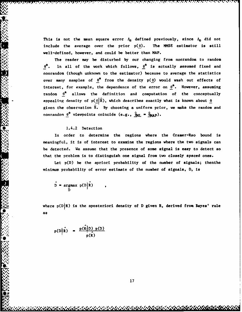
Let p(D) be the apriori probability of the number of signals; thenthe

minimum probability of error estimate of the number of signals, D, is

D = argmax p(D R)D!

'p 'p

where p(DIR) is the aposteriori density of D given R, derived from Bayes' rule

as

- (Di) - p(RD) p(D)

p(R)

17

* 'p0

-- -- - -. ;F 77 F. wr-

and the probability of error (PE) is

PE prob ( D*)

d

where D* is the true number of signals.

This detector is closely related to the optimal estimators, as will be

seen in Chapter 2.

1.5 Previous Work - Present Contribution

Research relating to optimal angles-of-arrival estimation has been

carried out since the early 1960's. None of the published results solve the

problem for our particular combination of assumptions, however. Most of the

work assumed the easier deterministic model, which implied also that just one

look was considered. Sklar and Schweppe [121 and Pollon [101 computed the

Cramer-Rao bounds for this problem, for various array configurations and two

signals. Young [17J assumed a prior density on 0 as we have and derived the

form of an analog signal processor for the MMSE estimator. Ksienski and

McGhee [81 considered the ML estimator for two signals and computed it

approximately by maximization over a finite 10 by 10 grid of directions.

Pollon and Lank fil] ran an analog simulation of the two signal ML estimator

for a certain circular array.

Gallop and Nolte [41 and Hodgkiss and Nolte [7J examined the one-signal

case only, considered mainly the detection problem. Rife and Boorstyn [13,

141 simulated the one- and two-signal estimators and compared them to the

Cramer-Rao bound, but approximated ML by a simple discrete Fourier transform.

The multiple look, Gaussian model problem is the more difficult one and

has been little examined. EI-Behery and Macphie [3] investigated the

one-signal ML estimator, which reduces to a discrete Fourier transform. They

performed an extensive Monte Carlo Simulation as we will here and found

attainment of the Cramer-Rao over a surprising range of SNR. Lainiotis [91

18

,%It V ~ -. V -. - " -11%7; V

considered the Gaussian model for Bayes' estimation in a control theory

Lontext. The estimator was computed by a maximization over only 10 grid

points, however, one of which was the true parameter value. Such a choice

probably explains the performance observed. A control theory or state

variable approach with finite grid approximations is also considered by Bucy

and Senne [21, in the context of the phase demodulation problem, and with a

thorough Monte Carlo performance evaluation.

The contribution of this report consists principally of the accurate

computation of performance of the MAP and MMSE estimators for Gaussian

two-signal, known powers problem. The calculation is accurate enough to

distinguish the unusual features of the Cramer-Rao bound mentioned earlier.

Additionally, the performance of the optimal detector is computed and

compared to an ad-hoc approximation based on the Cramer-Rao bound, and to a

rigorous known-directions bound.

In Chapter 2, a more detailed derivation of the form of the MAP and MMSE

J Pestimators and the optimal detetor for our problem is given. The chapterclosed with some example plots of p(O R) for two emitters. These plots

provide insight into the nature of the estimation errors.

In Chapter 3, the results of the performance evaluation are presented.

NFirst, error sources in the computer calculation are quantified and seen to be

acceptable. Then the results of the calculation are plotted and compared to

the Cramer-Rao bound and the PD bounds. The bounds' behavior is seen to

indeed be real.

In Chapter 4, the consequences of the tightness of the bound are

.discussed, along with suggestions for further research.

* The appendices contain derivations of the confidence intervals for the

Chapter 3 results and of the known-directions PD bound.

S.9

2.0 THE MAP AND MMSE ESTIMATORS AND THE OPTIMAL DETECTOR

In this chapter, the equations for the MAP and MMSE estimators and the

optimal detector are derived in detail. Although the derivations are classi-

cal 1151, some simplifications specific to the two-emitter problem are ap-

plied. The equations center on the expression for the aposteriori density,

* p(8 R), and the chapter is concluded with example plots of p(elR) illustrat-

ing some properties which have been derived or observed.

" Since p(e R) embodies all the information about e in R, it is an import-ant function itself in the angle estimation problem.

2.1 MAP and M4SE Estimators

As mentioned in Chapter 1, the MAP and MMSE estimates of the direction

parameters are given in terms of the aposteriori density p(Ojf) by

0 argmax pOR-iAP e

.-MSE - f f de 1 P(6IR)

The form of p(eV) now follows our Gaussian assumptions. We have first

(from Eq. (1.8)) that p(f116) is a multivariate Gaussian density with zero mean"and covariance R(8):

C . * ~ -1 e L r R (e ) R

fiiC-Je

To define the aposteriori density, we mast use the prior density of _, p(8),

defined in Chapter 1. Then, by Bayes' rule,

*The notation here is loose since this is actually p(Xie) is expressed in

.'.erm of R. R itself is Complex Wishart [5). This detail does not

- effect p(J).

20

U..

111! I 1 "151

P(.IR) - p()

p(i)

Since p(R) is independent of _, it is just a normalizing constant for the

density. Likewise, we chose a uniform prior density on 0 (in Chapter 1), so

that p(O) is also a constant. Therefore,

p~l)- K (RI6)

where K depends on R but not on 8.

We now absorb more constants by using a well-known matrix inversion

identity,

R_ (I + VvH) -I- VQVH

where Q (p-1 + W)-I

(same definitions as used for Cramer-Rao bound in Section 1.3), and get

p(eR) = K 1 R(O) 1 L e - Ltr (I - VQV)R

. K _NI. IR(_)I L e Ltr (R - VQVR)

= K' JR(6)I - L eL tr QV Hv

-NL -L trR

where K' - K - e is once again independent of 8.

Finally, the determinant can be reduced since we assume only two emitters

by

IR( )j " IVPVH + 1 (1 + X1 (1 + A)

+ X1 + A2 + A1 X2

21

N ~ N. N %~ \% ~ %% ~

W -.12 2 II_7_ - 1-" i** b e W- 2 _V Y

where X1 and X2 are the two non-zero eigenvalues of VPVH. By a theorem

from linear algebra, 1 1 and X2 are also the only two eigenvalues of

..t ' P v Hv " Thus,

XA1 + X2 tr(PVHV) tr(PW)

and

X1. 2 = IA2 - trPW )

implying

R(6~ I + tr(PW) + I PI

which is convenient since PW is only a 2 by 2 matrix. Therefore, we now have

P(eIR) K ' e L (2.1)--1 + tr (PW) + IPwI)L

This expression, unfortunately, cannot be solved analytically for its

maximum or mean, so numerical procedures must be used to compute 0 and

eiMISE. For our two-emitter known power case, e is only two-dimensional,

hence, such numerical procedures are reasonable. Of course, this was the

principal reason for limiting the investigation to this case. The procedures

used are described in Chapter 3.

2.2 Optimal Detector

The optimal detector, as also covered in the first chapter, is given by

* D max p(DIR)D

22

and is the minimum probability-of-error (PE) estimate of the number of

signals present. Since D must be determined without knowing the signal

directions, this is the composite hypothesis testing problem as defined in

[151, with e as the nuisance parameter. The test is seen to be simply

related to p(Oj ) of the previous section.

We assume as in Chapter 1 that the presence of some signal is easy to

detect, therefore we need only distinguish D-1 and D-2. Also, we assume that

these cases are equally likely apriori, thus the apriori density of D is

p(D1) - p(D-2) - 1/2. Finally, we must specify the known power if one signal

is present. The physically meaningful choice for this power is Pl + P2

where Pl and P2 are the powers when two signals are present. This choice

also should be the most difficult detection problem since otherwise one and

two signals could be distinguished on the basis of total signal power alone.

Now, by Bayes' rule,0!

" .p(RID) p(D)p(DIR) - D 1,2

p(R)

- K p(R ID)

since p(D) and p(l) are each independent of D. The constant K here is

unrelated to the K of the previous section.

Now, p(R D) is obtained from p(RID, 0) by

p(RID) - f de p(RID, 8) p(O) dO (2.2)

where the integral is one dimensional for D-1 and two dimensional for D-2.

• For D-2, p(RID, 8) is what we actually meant by p(Rje) in the previous

section, where two-dimensionality was implicit. Furthermore, p(RIDl, 0) is

obtained by evaluating the former along the diagonal 01=02,

p(RjD-1, 8) -(I-,01.

23

~- U.

l .V

. which simply says that one signal in direction e with power pl + P2 is

indistinguishable from two signals at the same direction 0 with powers Pl

and P2. Also, we take the apriori density of 8 for D-1, p(8), to be uniform

on -1 < 8 < 1, hence p(e) - 1/2. Therefore, plugging the above and Eq. (2.1)

into (2.2), we have

)I-L L tr QV( H ) D-1KI~ ~ ~ -1de-L)I

p(D f_) - p)eL (2.3)Qe H

according to whether the 1 dimensional or 2 dimensional integral of p R) is

larger.

The integrals are, as usual, intractable and must be computed

numerically. Integration procedures used will be described in Section 3.2.

2.3 Examples of Properties of p(81R)

The aposteriori density reveals precisely how much information about 8 is

contained in R and is the function in terms of which the optimal estimators,

MAP, MMSE, and detector can be expressed. Therefore, before examining the

statistics of the estimators in the next chapter, it is interesting to see

just what it looks like.

First, we see (Fig. 2.1) that for equal powers pl and P2, the pdf is

symmetric about the diagonal 01 - 02. This clearly must be true, since

the numbering of the angles as "1" or "2" is arbitrary. The positions of

21W and ._Q.MSE are also shown in the figure. Note that _M E in

particular must be computed by integrating only over the triangle, since the

mean of the density over the square (due to the symmetry) will always be on

the diagonal.

Another important feature we see is that extraneous maxima tend to be in

the form of ridges along the lines el - 01 and 82 02, i.e., one

24

AI

L = 5 LOOKSSNR = 5 dBN = 5 SENSORS

-0 = 2.000 BEAMWIDTHS

30od 20i101

1.00

0.75 0

0.50

0.25

.102 0. /-PMMSE

-0.25 -

a .MAP

-0.50-

-0.75.

-1.00 -0.75 -050 -0.25 o.i 5 0.0 0.75 1.00

61

Fig. 2.1. Exanmle of p(01R) for equal powers.

,2* 25

pU

,.

* angle correct and the other arbitrary. The ridges tend to disappear froia the

pdf as the number of looks increases (Fig. 2.2a) but, as can be seen from the

log pdf, which is the same as the log-likelihood function (Fig. 2.2b), are

always present to some extent. This property could confuse a gradient search

type algorithm for finding the

If P1 * P2, there is an ordering on the signals, say 1" is the

larger one. Hence, the pdf is not symmetric and should have a peak only on

. the correct triangle (Fig. 2.3). Notice that the peak is no longer

approximately circular. In fact, it is about 10 times broader in the e2

direction as the O1 direction, which reflects the greater uncertainty in the

smaller signal's location 02. Of course, if Pl is almost equal to P2,

the estimator will have difficulty distinguishing which is actually larger,

hence there will tend to be peaks on each triangle until many looks are taken

(Fig. 2.4).

Finally, we note that once the aposteriori density is essentially

f.. unimodel on the triangle, it can be well approximated by a Gaussian mound. In

fact, it is close to a Gaussian with mean given by the true signal locations

0" and variances given by the Cramer-Rao bound (Fig. 2.5). Notice that the

.-- grid has been shrunk in this figure to a small region about the peak.

...,2

0.

i_.'. 26-

PM-I r. In' W. IFI7b 7077777 -J 'Y v

'6

SNf 5 dBN = 5 SENSORS

1000 = 2.000 BEAMWIDTHS

750,

250

* 0

-050

.106

1.00'

0.75-

0.50.

0.25-

02 0-

-0.25-.

% -0.50

d%

* -0.75

-1.001_ _ _ _ _ _ _ _ _ _ _ _

-.00-0'75 -0.'50 -0.25 0 0.25 0.50 0.75 1.00

Fig. 2.2a. p(8 R) for additional looks.

27

M iI

L =30 LOOKS

1p, SNR 10 dBN =9 SENSORS40 2.000 BEAMWIDTHS

0-10

0 -300~0

02

* ~. 3300

Boo50

-10 07 05 02 .5 05 .510

.' o,

Fig 2.b 1%d lusrtn igs

U2

125 L = 5 LOOKSSNR = 15 dB

1,0 PI /P2 = 10 dBN =5 SENSORS

40 =1.000 BEAMWIDTHS75

.ft-f

500

25

0

0.5 0.5

0 0

-1.0

Fig. 2.3. Example of p(O R) for unequal powers.

100 L = 5 LOOKSSNR = 10 dBP1/P2 = 1 dB

75 N = 5 SENSORS40 = 1.000 BEAMWIDTHS

~25

0

.0.

6 -1.0

f Fig. 2.4. Example of p(e R) for almost equal powers.

29

Oki

III

L = 10 LOOKSSNR = 20 dBN = 9 SENSORS

TRUE PDF A = 0.100 BEAMWDTHS

7500

2500-

0,

0 --. ,,o

-0.04J0.0

ooo GAUSSIAN APPROXIMATION

0 02 002

0

02 -002 - 002 01

Fig. 2.5. Coqparison of p(eI R) to Gaussian pdf with Cramer-aobound an its covariance.

$30

3.0 MONTE CARLO PERFORMANCE EVALUATION

In this chapter, we present the results of the Monte Carlo evaluation of

the performance of the MAP and MMSE estimators (their rms errors) and of the

optimal detector (its probability of detection, PD). The computational pro-

cedure and its sources of error are first described. The errors arise fromA

two sources, the piecewise constant approximation to p(8IR) and the finite

number of Monte Carlo trials performed. The results of the evaluation are

presented next and compared to the Cramer-Rao bound. The main result is that

*c the rms error of the estimators achieves the Cramer-Rao bound wherever the

PD is usefully high and deviatos from the bound only for low PD, where the

estimates become biased. This result is surprising due to the bound's unusual

behavior.

3.1 Computational Procedure

Simple approximations were used in the computations of performance to

make the program fast and to make the errors easy to understand and quantify.

The following sections describe first the rms error calculation and then the

P0 and bias calculations.

3.1.1 RMS Error Calculation

The conditional error covariance of an estimator 0 6 0(R) is, by defini-

tion,

i* E 83*) (6 - f dAtp(_ e*) (6 -e *) (j -e*) (3.1)

where * is the true theta value. The estimator's rue error on the ith

direction is the square root of the ith diagonal element of Ae,

o (Aeii

31

All....... v

In order to numerically compute Ae from (3.1), we must make basicallytwo different approximations. One is the approximate computation of 6 given

.. ;..an accurate R and the other is the approximate integration with respect toX

"over its density. The approximations used and their errors will now be de-

", scribed.

Given an Rthe two estimates 8'MAp and ^_MMSE8 are computed as

i follows. First, p(6_IR)/K' (Eq. 2.1) is evaluated over a fixed finite grid of

'. b. e values, say G by G, uniformly spaced over the square (see Fig. 3.1). Since

for high SNR or large numbers of looks p(O XK) is zero everywhere except in a

hii

small region around 6" the square is taken to be the smallest one which

safely encloses the pdf's support. This is actually 1-1, I] x [-I, I] onlyfor the low SNR cases examined. Then this is numerically integrated over the

upper triangle to find K . OMMSE is now the numerical integral of _p(e )

over the triangle and ohe is the location of the grid point with the

largest value of p( T). The integrals are taken such that they are exact if

p(e_ R) is assumed to be piecewise constant, i.e., constant on each grid cell,

as shown in Fig. 3.1. This implies that the computation is a simple summationplus a few correction terms and that the only error source is the degree to

which p(O R) is not piecewise constant. The error will go to monotonically

zero as G is Increased since this approximation converges uniformly on the

p: , square to p(_eI x) [2].i! In f act, a plot was made of the integrals versus G to determine how fine

"j a grid was required (Fig. 3.2). For typically smooth true pdfs, G > 50 was

':adequate for an accuracy of about 2% of the true value. Errors in aMSE and

, _MPwere not surprisingly of the order of the grid cell size. Making theseerrors about 2% places them below the errors due to the second source, the in-tegration with respect to R.

IThis integration, involving as it does the complicated function

p(e is hopeless to perform analytically. It is also of such dimension-

ality (e.g., 81-dmensional for nine antennas) that the only tractable_numerical integration method is the Monte Carlo method [16.

32

1.0 ......

I~I

0.5-....

02 0 GRID POINT

.. . .. .. ~~~~~ ~~~... .. . ... .. .. .. .. . . . . . . . . . . .

R EG IO N O F .....

~~~~~~~~~~. . . . . . . . . . . . . . '. ... . . . . . . . .-. . . : .

...... ... I.N EGO.......... IN-0.5

-1.0 -0.5 0 0.5 1.0

2-

X0 01CL

'CV

.1.

APPROXIMATE pdf = TRUE pdf AT GRID POINTS

4 Fig. 3.1. Piecewise-constant approximation.

4 33

a. o- :: : :: : :: : : :: : :: :. ... ..... ........ ........

p..

125

120

115. 1/K'

UJ 110-

0uJI-

q Ui 100-

o,.

95 OMMSE,2

90 1,10 15 20 25 30 35 40 45 5 55 0 65 70l

GRID SIZE, G

Fig. 3.2. integrals versus grid size, G.

34

Monte Carlo integration in this case amounts to the simulation of the

estimators, computation of the errors and squared errors, and accumulation of

their sample means, i.e.,

MT

e = I IO(Ri)- e )e M i-1 - ---

where M is the number of statistically independent Monte Carlo trials, Rj is

the sample covariance chosen from the population p(RO*) on the ith

trial, and Ae is the estimated error covariance.

Now Ae is a random variable with some unknown probability density. Its

expected value is the true Ae and its variance is determined by its pdf. If

we assume that its pdf is Gaussian, which will be approximately true for large

M, then its variance can be computed and used to compute the number of trials

required for a specified accuracy. Choosing a 99% confidence interval width

of ±2 dB as adequate for distinguishing the interesting features of the

bounds, we found by making trial runs that about 1000 Monte Carlo trials were

required (see Appendix A).

Since the rms errors for each direction eland 02 are equal by symmetry,

the final estimate of the rms error for either direction was taken to be

a 1 + 022

where

3.1.2 Probability of Detection Computation

The probability of detection (PD) for the optimal detector is given by

- y dl p(Ij6*) (3.2)* 0

0

35

0. le.WN~ IL

where

£ - S f S1 d81 de2 p(OIR) -S 1 d6 p(()R) (3.3)-1 6 -1

and p(JE_) is I's probability density. So PD is the probability that the

integral over the triangle is greater than the integral along the diagonal.

Unfortunately, p(X e*) is not tractable to compute analytically and

probably not easy to integrate as required in (3.2). So PD must be computed

by a Monte Carlo simulation*.

We define the 0-1 random variable

0" 1 <' 0 (3.4)-.. 1, 1 > 0

i.e., 1' 1 1 iff two signals are detected. Then PD is the expected value of

PD E(4')

'-J

Therefore, PD can be approximated by

P =1' (3.5)

where M is the number of statistically independent Monte Carlo trials, as

before, and £1 is a sample of 2' from the population of p(I'1*) on the

ith trial. Xj is generated, of course, by computing p(e IRi), finding its2-D and 1-D integrals as in (3.3), and using the definition (3.4).

. .45

-.. ..

*If it is assumed that the detector knows e*, then this PD can be computed., and serves as a convenient upper bound for the present one (see Appendix B).

".

36

.5V

-7.7-T -2 .- a- ff - .

The approximations made here are in the piecewise constant approximation

for p(OIR) in the integrals and in the finite variance of the random variable

PD. Assuming the grid has already been chosen fine enough to make the inte-

grals for the rms error calculation in the previous section sufficiently accu-

rate, only the Monte Carlo error remains.

As explained in Appendix A, this error is quantified by the observation

that PD has approximately a Gaussian pdf. Using the 1000 trials required

for the ras error calculation, we find in the Appendix that the 99% confidence

interval for PD is about + .05.

3.1.3 Bias Computation

'.. The bias b of an estimate e is defined as

b - E(O - 0)

- and was computed for MMSE and MAP exactly the same way as the rms error and

the probability of detection. Given H sample angle estimates, the estimate

for the bias was

m1 '-" M

Confidence intervals for b follow easily and are derived in Appendix A.

3.2 Results

A computer simulation program was written which performed the Monte Carlo

evaluation of rm errors, probability of detection, and bias of the optimal

estimators (MAP and MMSE). The results of running that program for various

array signal-to-noise ratios, emitter separations, and numbers of looks are

presented in this section. In every case, two equal power, uncorrelated emit-

ters and a uniform linear aray with nine or five elements were assumed. The

results indicate that rms errors and detection thresholds corresponding to the

Cramer-Rao bound are in fact achievable given as few as 10 looks at the array.

37

%

N

Incidentally, the running time for the program for 9 elements and a 50 by

50 grid was about 0.19 sec/trial on an Amdahl 470 and 3.1 sec/trial on a VAX

11/750.

3.2.1 RMS Error Results

Figures 3.3a through 3.3c show the computed rms errors of the MAP and

M SE estimators versus SNR for emitter separations of .1, .o/T, and .01

beamwidths, respectively, and all at 10 looks. Figure 3.3d is an overlay of

3.3a, b, and c. The array for these cases has nine elements implying a beam-

width of 2/9 - .222. For an emitter separation of Ae, the true signal loca-

.. tions were taken to be

1

0* - A

2 2

i.e., centered on the array boresight.

'.e- Below about 5 dB in SNR, we see from the figure that the rms error is in-

dependent of the true signal separation. In fact, it is independent of almost

everything in this region since the aposteriori pdf is approximately uniform

over the triangle, on the average, implying that the estimates vary approxi-

mately uniformly over the triangle. An exactly uniform pdf would imply an rms

error of 4.5/,/'w 2.6 beamwidths, approximately that of MAP. MMSE is somewhat

' better since it tends to choose estimates in the center of the triangle given

a uniform pdf, and this happens. to be close to where the signals actually

are.

Above about 20 dB is the more interesting region of SNR. First, we see

that the MAP and MMSE estimator errors are identical. This is not surprising,

since the aposteriori density is substantially unimodel and symmetric about

38

-po

4. 10

KNOWN POWERSEQUAL POWERS

1 L = 10 LOOKSN = 9 SENSORS

MONTE CARLO POINTS0.1 0 MAP

x MMSE

99% CONFIDENCE0.01 C INTERVAL WIDTHCRAMER-RAOBOUND

0.0017 0 =0.1 BEAMWIDTHS

E 0.000,

(a)cc0cc¢ 10"* D 2 Signals

to KNOWN POWERS0 EQUAL POWERSx L = 10 LOOKS

N = 9 SENSORS

MONTE CARLO POINTSoA o MAP

x MMSE

099% CONFIDENCE0.01 CRMR\RA[1 INTERVAL WIDTH

CRAMER -RAO

BOUND

0.001

.10 00316 BEAMWIDTHS

0.0001 ____________________________________

-10 0 10 20 30 40 50 60 70 s0

ARRAY SIGNAL-TO-NOISE RATIO (dB)

(b)

Fig. 3.3. Comparison of MAP and MMSE estimator accuracies withCramer-Rao bound.

.3

0 2 SignalsKNOWN POWERS

10 EQUAL POWERSL 10 LOOKS

0 N N 9 SENSORS

MONTE CARLO POINTSO MAPX MMSE

0.199% CONFIDENCE-- INTERVAL WDTH

O4Ol

0'01 CRAXMER-RAO,

0.001

. 0.001

ca (c)w D 2 Signals0 KNOWN POWERSE 10 EQUAL POWERS

L =L10 LOOKS

o)** N = 9 SENSORS

. , ,MONTE CARLO POINTS% * 0MAP

.1 \X MMSE

I99% CONFIDENCE* . INTERVAL WMOTH

0.01 CRAMER-RAO BOUNDS "...

0.001 0.1 *EAMWIDTS,• O0 1 0= 0.01 BEAMOTHS

.. .... ... .. .. . .. .. .

0.0001- -

-10 0 10 20 30 40 50 60 70 SO

ARRAY SIGNAL-TO-NOISE RATIO (de) .

a. (d)

Fig. 3.3. Continued.

40

its mode in this region, so that its mean and peak coincide. More signifi-

cantly, we see that the rms error is always less than or equal to the Cramer-

Rao bound (when less, the estimator was biased) and tracks the bound closely

beyond its first "knee," which we will later see is for (L-10) at the detec-

tion threshold. At 40 dB SNR, for example, we see that the rms error is

clearly (including the confidence interval) smaller for the smaller separa-

tions, verifying this unusual behavior of the bound noted in Chapter 1.

Additionally, we see that the rms error is approximately constant as the SNR

increases from, for example, 50 to 70 dB for the .01 beanwidths emitter sepa-

ration, verifying the plateau in the bound. Therefore, these counterintuitive

aspects of the known powers Cramer-Rao bound observed in Chapter 1 apply

equally well to the behavior of the optimal estimators. It was not "Just a

bound" after all.

*Of course, the preceding observations are for 10 looks, but this is a

C. surprisingly small number: the convergence of the rum error to the bound asr.%

the number of looks increases is quite rapid. Figures 3.4a and 3.4b show thisconvergence for two selected SNRs and separations, 50 dB, .01 beamwidths, and

30 dB, .1 beamwidths, respectively. The bound is achieved to within the 99%

confidence interval after about 10 looks and continues to track the bound forJ._U,

higher numbers of looks.

* . Expecting that the number of looks required to achieve the bound may be

related to the number of antennas, a run was made at 50 dB, .01 beamwidths for

only five antenna elements (Fig. 3.5). As can be seen from the figure, the

threshold is about the same as for nine antennas. It could be that the

threshold depends on the number of signal directions one is trying to esti-

D mate.

3.2.2 Probability of Detection Results

Figures 3.6 and 3.7 show the probability of detection computed versus SNR

for the same three separations and the same number of looks as used previous-

ly. From these plots, we see the region of SNR for which the rms errors are

of any practical interest.

41

0.01-

4

X4-A

E MS

0.0

E0.00 .1BEM ID

.10.1

NUBE OFUA LOOKSRSAO = 1 BEAWID.H

0 MS

I 42

0.0 ."d

*1 100.~ - %''i%

d A I C ~ M -c.INUMBER- OF' LOOKS

a ~ ~ ~ ~ ~ 7 j :6- 3*. *- s . a . -A-.

0 .1 D 2 S I G N A L S_ _ _ _ _

.. EQUAL POWERSAO = .1 BEAMWIDTHS30 dB ARRAY SNRN = 5 SENSORS

MONTE CARLO POINTS

'5. E

0

NUMBMREF-ROOK

Fi.35 ovrec fMPadMSEetmtr ihnme flos

43/

A1.0- 1 4F

D z 2 SIGNALS IKNOWN POWERSEQUAL POWERS

°8- L = 10 LOOKS EMITIER0 N = 9 SENSORS " SEPARATION

/" . (Beamwidths)/ 00.:

U. .

0.10 99% CONFIDENCE

I J INTERVAL WIDTH:30.4-

4 CRAMER-RAO0PPOX MONTE CARLO

POINTS0.2

-10 0 10 20 30 40 50 so 70

ARRAY SIGNAL-TO-NOISE RATIO (dB)

Fig. 3.6. Comparison of optimal detector performance to Cramer-Rao

'p.deie aprxmain

04

-1 0 2 0 0 5 0 7

• .-.- " ,",. - " ARRAY- SIGN-TO-OIS RATI (dB"') ;

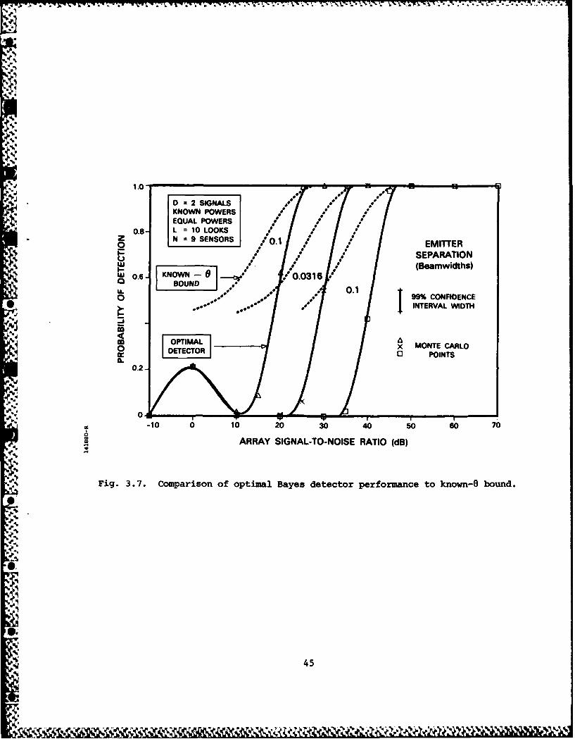
1.0-D 2 SIGNALS *KNOWN POWERSEQUAL POWERS */

0.8 L = 10 LOOKS * *- N =9 SENSORS /0.1 / EMITTER

** * SEPARATIONU 0 . ,,w,(Beamwidhs)

0 KNOoo31 .BOUND

L°. . 0.1 Io0*,, 99% CONFIDENCE>.. o°- .°°INTERVAL WIDTH

0OTEMO x MONTE CARLO0E T 0 POINTS

0.2]

a..

. 0. 50T-(: ,0

-10 0 10 20 30 40 50 6 70

.,ARRAY SIGNAL-TO-NOISE RATIO (dB),-,-

Fig. 3.7. Comparison of optimal Bayes detector performance to known-0 bound.

.5?

44

%0 %1

7 1 77 -, -. - X

Below 10 dB in SNR, we see that the PD does not depend on the true sep-

aration, as was the case for rms error. The detection here is probably no

better than a random choice.

At higher SNR, we see sharply defined detection thresholds which, in

fact, occur at the point where the rms error began to track the Cramer-Rao

bound. If we take the threshold to be when PD > .5, then a simple for.ula

based on the figures for the threshold SNR versus separation is

V.O

Detection Threshold SNR a -- (3.6)~(Ao) 2

where AO - emitter separation in beamwidths, valid for L - 10 looks. This

formula yields 20 dd, 30 dB, and 40 dB SNR for .1, .01 /_0, and .01 beamwidths

separation, respectively.

The dotted curves in Fig. 3.6 are an ad-hoc approximation to PD based

on the Cramer-Rao bound. They were generated by assuming that p(O_ t) was

Gaussian mound with -man given by e and covariance given by the Cramer-Rao

bound for the separation and SNR used. The integrals of the density over the

upper triangle (call this 12) and along the diagonal (II) were evaluated

exactly as in Eq. (2.3). The approximation to PD was then taken as

12P D "12 + I

Although this derivation is loose, here we see that it works quite well.

This implies that the aposteriori density is fairly well approximated by aGaussian mound with the Cramer-Rao bound as its covariance. This is also say-

ing that the off-diagonal term of the Cramer-Rao bound is being achieved,

since it corresponds to the orientation of the Gaussian mound, hence to the

relative values of 12 and 1l and thus to the PD. Such was expected from

examining the picture of the pdf for various cases, as in Fig. 2.5.

46

9~I

In Fig. 3.7, the computed PD'S are compared to the known 0 PD men-

tioned in Chapter 2 and derived in Appendix B. It is indeed an upper bound,

although not a very tight one. The known 0 curves also follow the 1/(A0) 2

dependence in Eq. (3.1) closely, indicating that knowing e is equivalent to a

fixed gain in SNR, independent of separation.

In Fig. 3.8, PD is plotted versus the number of looks, for the same two

cases as in Fig. 3.4. The threshold here is at about five looks, which agrees

fairly closely with the threshold observed for the rum error to achieve the

bound.

3.2.3 Bias Results

In Figs. 3.9a through 3.9c, the bias of the MAP and MHSE estimators ver-

sus SNR is plotted as a percentage of the rus error. Below -20%, one can con-

sider the estimator unbiased since the bias affects the rms error only by

(.2)2 - 4%. From the plot, we see that the estimator is indeed biased, as

it must be, in the low SNR region where its rums error was below the Cramer Rao

bound, but becomes unbiased at about the detection threshold.

The confidence interval shown is so wide because it was taken as the

. maximum (most conservative) estimate, i.e.,

upper limit = 100% • upper bias limitlower rms error limit and

lower limit - 100% * lower bias limitupper rms error limit

47

J

.to

%1.

D = 2 SIGNALS0.8 EQUAL POWERS

40 = .01 BEAMWIDTHS50 dB ARRAY SNRN = 9 SENSORS

0.6

I CONFIDENCEINTERVAL WIDTH

~0.40.4

MONTE CARLOCj0 POINTS

0.2

z* 0

I- (a)L)LU1- 0U-0

1.0

m D = 2 SIGNALS

0 EQUAL POWERSIo. IG .1 BEAMWIDTHS

30 dB ARRAY SNRN = 9 SENSORS

0.6 99% CONFIDENCE

0. INTERVAL WIDTH

MONTE CARLO0 POINTS

0.2

(b)

0 J- III I10 100

NUMBER OF LOOKS

Fig. 3.8. Performance of optimal Bayes detector versus number of looks.

48

• . ,,, *

100,D 2 SIGNALS

N KNOWN POWERSEQUAL POWERS

SO L = 10 LOOKSN = 9 SENSORS

AG= 0.1 BEAMWIDTIIS

-60 MONTE CARLO POINTS

40

20 ~ .~99% CONFIDENCEINTERVAL WIDTH

* (a)z 01

.1 100,ILD =2 SIGNALSKNOWN POWERSEQUAL POWERS

80L = 10 LOOKSN = 9 SENSORS

AG= 0.0316 SEAMWIDTHS

60MONTE CARLO POINTSX MSE

404

20 99 CONFIENCE% INTE.AL..T

* 49

... .. ..

D 2 SIGNLS

.. ........ EQUAL POWERS... .. L =10 LOOKS

N 9 SENSORS....... AO 0.01 BEAMWIDTHS'

60: MONTE CARLO POINTSI- VNMSE

* U OMAP

.~. . . ... .

LU

2Fig 3.9 .C.n.in..d.

.. .. :-N: :

'p0.

'4 50

7-K ---- 7' K7T

.. 4.0 CONCLUSIONS AND RECOMMENDATIONS FOR FURTHER RESEARCH

The most important result of this research is the presentation of the

agreement between the rms errors of the optimal estimators and the known

powers, Gaussian signal Cramer-Rao bound. The two unusual features of the

bound, that the ros error is constant over a range of SNR and is smaller for

44-S larger emitter separations over about the same SNR range, have been verified.

The verification was made rigorous through the use of a straightforward

finite-grid computation for the MAP and MMSE estimates and through the evalua-

tion of statistical confidence intervals for Monte Carlo results.

As a consequence of this agreement, the Cramer-Rao bound can be now used

with some confidence to predict the ultimate performance of angle-of-arrival

estimators for various combinations of assumptions. This is valuable since

.'- the bound is considerably easier to compute than the optimal estimator per-% .formance. One application of this was the ad-hoc forula for the PD derived

from the Cramer-Rao bound in Chapter 3, which agreed well with the PD corn-

puted by the simulation. Without running additional simulations, the bound

can be used for cases of different numbers of sensors, looks, or different

array configurations from those run in this research to predict performance.

The unknown powers Cramer-Rao bound may even be used, with some confidence, a

case for which the simulation is considerably more difficult, requiring a

4-dimensional grid.

-* Although it was the non-random param ters Cramer-Rao bound which was

actually verified, a random parameter (Bayesian) approach to the overall esti-

mation problem was used in order to define the MMSE estimator, for one, and.. -

more importantly the aposteriori density of the directions-of-arrival

p(8R). The properties of this function are important since they could lead

to efficient procedures for computing the optimal estimators and to insights

into the sources of estimation errors.

While the known powers problem is certainly of theoretical interest,

isolating as it does the difficulty in angle estimation alone, it might not be

of great practical utility. Further research should therefore center on the

. unknown-powers problem. This research could be approached in several ways.r W4

%z4, LVL

A straightforward extension to a 4-dimensional grid search is, of course, not

computationally feasible. One could test the importance of knowing the

powers by providing the known powers estimator with incorrect powers, which

would determine how finely tuned the estimator is to the particular signal

model assumptions. If it is not very sensitive to misinformation about

powers, then one would expect completely unknown powers to cause little

additional degradation.

Extensions of this research to even more general cases, such as > 2

signals or to 2-dimensional angles parameters, await sophisticated but

provably accurate procedures to search a many-dimensional space. Our

restriction to just two known power signals was made specifically to avoid all

questions of convergence which typically arise with such procedures.

Hopefully, the results presented here will be of some help in the general

problem.

The plots of p(6 R), for example, provide some insight into the animal

which must be searched. The fact that p(01R) seems to approach a Gaussian

mound with the Cramer-Rao bound as its covariance, if quantified, could be

used.

V.

€. 52

t

ACKNOWLEDGEMENTS

I must thank Ken Senne and Dick Bucy for suggesting the present problem,

rescuing me from a previous intractable one, and for guidance throughout the

research. Thanks to Jim McClellan for many helpful discussions and much pa-

tience as my advisor. Thanks also to Russ Johnson for technical suggestions

and moral support and to Diane Young for excellent typing on a recalcitrant

. word processor. Finally, I thank Lincoln Laboratory for its generous sup-

- port over my years as a research assistant there.

.5J.

!%d' •

-.

.i

53

17 .7, 7 ... ..

REFERENCES

1. R. S. Bucy, C. Hecht, and K. D. Senne, An Engineer's Guide to BuildingNonlinear Filters, Vol. 1, Frank J. Seiler Research Laboratory (AFSC),USAF Academy, Colorado, 1972.

2. R. S. Bucy and K. D. Senne, "Nonlinear Filtering Algorithms for VectorProcessing Machines," Comp. & Maths. with Appls. 6, 317 (1980).

3. I. N. El-Behery and R. H. Macphle, "Maximum-Likelihood Estimation ofSource Parameters from Time-Sampled Outputs of a Linear Array," Journalof the Acoustical Society of America 61, 125 (1977).

4. M. A. Gallop and L. W. Nolte, "Bayesian Detection of Targets of UnknownLocation," IEEE Trans. Aerospace and Electronic System AES-1O, 429(1974).

5. N. R. Goodman, "Statistical Analysis Based on a Certain MultivariateComplex Gaussian Distribution (An Introduction)," Ann. Mathematics and

* Statistics 34, 152 (1963).

6. D. F. DeLong, '"Multiple Signal Direction Finding with Thinned Linear

Arrays," Project Report TST-68, Lincoln Laboratory, M.I.T. (13 April1983), DTIC AD-A128924.

7. W. S. Hodgkiss and L. W. Nolte, "Bayes Optimum and Maximum-LikelihoodApproaches in the Array Processing Problem," IEEE Trans. Aerospace andElectronic System, AES-Il, 913 (1975).

V 8. A. A. Ksienski and R. M. McGhee, "A Decision Theoretic Approach t. theAngular Resolution and Parameter Estimation for Multiple Targets," IEEETrans. Aerospace and Electronic Systems AES-4, 443 (1968).

9. D. G. Lainitotis, "Otpimal Adaptive Estimation: Structure and Parameter

Adapatation," IEEE Trans. Automatic Control AC-16, 160 (1971).

10. G. E. Pollon, "On the Angular Resolution of Multiple Targets," IEEE* Trans. Aerospace and Electronic Systems AES-4, 145 (1967).

11. G. E. Pollon and G. W. Lank, "Angular Tracking of Two Closely SpacedRadar Targets," IEEE Trans. Aerospace and Electronic Systems AES-4, 145(1967).

54

REFERENCES (continued)

12. J. R. Sklar and F. C Schweppe, "On the Angular Resolution of MultipleTargets," Proc. IEEE 52, 1044 (1964).

13. D. C. Rife and R. R. Boorstyn, "Single Tone Parameter Estimation from

Discrete-Time Observations," IEEE Trans. Inform. Theory IT-20, 591(1974).

14. D. C. Rife and R. R. Boorstyn, "Multiple Tone Parameter Estimation fromSDiscrete-Time Observations," BSTJ 55, 1398 (1976).

15. R. L. Van Trees, Detection, Estimation, and Modulation Theory, Part 1(Wiley, New York, 1968).

16. S. J. Yakowitz, Computational Probability and Simulation, Chapter 6 (AddisonWesley, Reading, 1977).

17. G. 0. Young, "Optimum Space-Time Signal Processing and ParameterEstimation," IEEE Trans. Aerospace and Electronic Systems AES 4, 334(1968).

18. S. S. Wilks, Mathematical Statistics (Wiley, New York, 1962).

55

APPENDIX A

CONFIDENCE INTERVALS FOR THE MONTE CARLO RESULTS

In this appendix, we derive the confidence intervals for the estimates of

bias, mean square error, and probability of detection shown in the figures of

Chapter 3. Much of this appendix is abstracted from Chapter 4 of [1].

Let a be the true value of some parameter to be estimated and let a be

its estimate. Then a 100y % confidence interval for a is a pair of random

variables £(a) and u(&) such that

prob (X(a^)< a < u(a^)) - Y

118, p. 365). Here we choose the symmetric interval where I and u are of the

form

X(M^) = -kU a-

u() a + k

thus,

prob(la- a < k) =y

To compute k, it suffices to know the pdf of z - 'a - a, say p(z). This

implies that k is given by

kf dz p(z) -Y-k

In each of our cases, we are estimating the mean R of a random variable x

given M independent samples {xj, " ° "' i} of that variable. Hence, the

best estimate of x is

57 B1sqL AN K

If we assume now that M is so large that x is approximately Gaussian, then k -

R is Gaussian with mean, variance given by

E(x - X) -xi ) - x =0=~ E~x) _ xi

a var(x) E(x2) - x = var(x)M M

and we can easily derive a symmetric confidence interval. In particular, the

99.74% confidence interval is given by

Unfortunately, although the pdf of * may be very nearly Gaussian, the pdf of x

is unknown so a2 is also unknown. Here, we get an approximate confidence

interval by using the estimate of a2

2 1 2 -2a - txi -x

which should be a good approximation for large M.

* For bias b and mean square error s, we are estimating the means of

x=-eand S * 2

x e-O )2

respectively. Hence, given M sample angle estimates Je1,...,M}, we

compute the estimates

M *

I * 2

..58

^ 4

U4 = -i

implying that the approximate 99.74% confidence intervals as derived above are

s- a s f

The interval for the rms error, V, was derived from the interval for s as..

On the plots, all of the intervals (for each SNR and separation) were

approximately the same so the largest one was taken as the interval for all

the points. By making runs for various values of M and computing the

confidence intervals, M-1000 trials was found adequate for a ±2 dB interval

for ra error.

For the probability of detection, we can be a little more precise since

we are estimating the mean of a binomial random variable

0, no detection, probability 1 -PD

1, detection, probability PD

and can compute the worst case var(x):

vat(x) E(x 2 E(x)2 . P - P2 . PvU - p

1 1 1

2 - T for all O< PD_< Iimplying

var(D)<

D59

5. 59

Therefore, the worst case 99.74% confidence interval for PD is (stil'

assuming PD is approximately Gaussian)

I^D -DI <2vg1'

which, at M - 1000 is

- DI < .0474'

as shown in the PO plots of Chapter 3.

%;

a-60

-. - -- - - - - - . . .

* APPENDIX B

THE KNOWN ANGLE-OF-ARRIVAL DETECTOR

The probability of detection (PD) of the optimal Bayes detector

described in Chapter 2 can be upper bounded by the PD of a detector which

knows a priori the angles of arrival e. This latter PD, unlike the former,

may be computed analytically and hence is a convenient bound. In this

appendix, we derive in detail the PD of the known e bound, which is seen to

be the solution of the general Gaussian hypothesis testing problem in [151.

By the phrase "known e," we mean more precisely that if there are

actually two signals present (hypothesis H2), we know their angles

0616= (12)2

and if there is only on- signal present (hypothesis HI), we know its angle

0. Of course, we assume throughout this report that the powers of all the

signals are also known, say pl and P2 for two signals present, and p for

one signal. Normally, for the problem to make physical sense, we assume

iP =P1 + P2

0 - 0l + P22 (center of power).p1 + P

Knowing the angles and the powers now means that we completely know the

covariance of the observations [x}Ji. 1 on each hypothesis. Therefore, the

detection problem is to discern based on the L independent samples La}i=I

whether

61

R. -1 :N (0, R,)

or

H 2: ac. CN (09 R 2)

where

R I + PLV(6) v(e)H

' (B.2)

R 2 I+ V6) PV e)H

P Pi 0

00

vi(e) - direction vector

v~)- (ed~ M(Y2)

CN(m, R) - complex normal pdf with mean m and covariance R.

This is the weil-known equal mean, differing covariance Gaussian hypothesis

testing problem [15, p. 113, case 1C]. The computation of its PD is

tedious, but straightforward.

The likelihood ratio test is

L ~ H2

P({!il~ 111) 2(B.3)

62

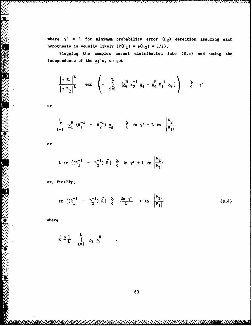
where y' - 1 for minimum probability error (PE) detection assuming each

hypothesis is equally likely (P(HI) - p(H2) - 1/2).

Plugging the complex normal distribution into (B.3) and using the

independence of the x ls, we get

7rR iL L H -I R 2IL e1 2 E Z i R11 1 <

illor

L H (-1 R-1 2

1, n y' +L n]4

or, finally,

tr ((R - R 1 ) >) ' - --., +)n / (B.4)

where

LI'L :i_=ii-i

.-

Let

'.I tri(Rl 1 R 21 ) R^)

be the statistic and

R n y'2

L +R

be the threshold. Then the PD of this test is

PD = prob(I > y) - f pi(uIH2) duDY

where pj (-) is the pdf of t, which will be obtained through the

characteristic function of 1.N The characteristic function of X,

-4, (jw) E(eJ £)

is given on hypothesis Hk by

ox (jW1 H) 1 w Rk (R- 1 - R21) -L

as derived in [5, Lemma 4.11. Pulling out an IC,2

1 1tl/2 -1; 1;),/2i L09 (.WH k) -1 - 1w P/ (RI - R) R

64

4j

S:

Now let

U NJ - /2 (RI - R 2 ) li (B.5)

be the eigenvalue decomposition of the Hermetian matrix on the right-hand

side. Then,

---L

.1W A l

L -L

III JAL -I

- det kli n

1 1W

.1* (-1lI ) " . L~ ("-Ln

LH ( ) L I (I L A L

This is a difficult characteristic function to invert until we note that only

three eigenvalues are non-zero since

4.

'I.

~* - - - - 7 -77 - - --

rank 1~/2 (R- 1 -1 1/2 ran ( - 1(i 1 2iLk rank 1 - 2 )

= rank (I - q v v (I V Q V9))

- rank (V 0 - q vv)

3 at most.

Now

'Pt (LsIH k ) (- )L - L - L - L

X 7 (s- ,j1) (s- ,2) (s-)3)

which may be expanded into partial functions

1 3 LLL I ij (B.6)

I XLL j-I 1-1 (s- b)1 2 3

where bj - l/Xj and the coefficients aij are given by

(-I)L dLi L

a (L - I)] dsL-i [(s - b2 ) L (s - b3) -L

ds=bI

(_)L L i (-1)( (L + 1- I)! b 2b (L + 9)(L- i) (L - I)! 1 2

km0

_)L-t-L (L+L-i-£-I)(-1)! (l - b3-(L+L-i-L)

(-)CL -1)F! (b b 3 )

66

.M

-2L- L-i b - b3

(L - i)! (bI - b2)L (b1 - h3)2L-i k=O 1 - 2

(L-iI (L+t-I (2L-i-L-1)!

!(L-i-gE)! (L-1) 12

or, finally,

(b3 - b1) L-ia i - L TL I u.,ri

(bI - b2 ) (b3 -b 1) L-0

where

' r = 3 -1 l , °T (2L - i - 1)! (2,L-_£-1 1

b2 U -I (- L 1 1L L

u (L + I - I)! (2L - i - - I)! . (L + 1 - 1) (L - I - .+ 1)1" i! (L - i - I)! (L - 1)12 i (2L - i - A)

and a1 2 and a13 are obtained symmetrically.

Given these aij, we now inverse transform Eq. (B.6):

pit") -Ffop(JwIHk)

L ~ 3 L --~ ~ 1 a1 j F11jw-

.1(A 1 X2 A3 )L j.-i 1,X

SD- L 3 U00), A1 > 0 -I/ La(L1(A ( 2 X3) L J(- I <05

67

-. i b *t *-*. ._. - -*! . .*.% . ..*.,*-.•

.. ,. :,* d ... w .. . -.. . ~ i

Therefore,

L L 3 L a u(x) AP f dx p£(x) - Lf dx I }(x) } (Lx) e

A2 ))L 7 1 -)1 -u(-x

- or

. -.

aD AlI (B.7)(X I Ix2 X 3) L Jul -11 aiJ j I i j (B )

where

Ly(sgn A) (sgn -y)r~i, -j

S0- +1 + -

Pi + +

and P (, .) is the incomplete Gavma function

1n x) -F n-i -t.P f dt t e -

N.. 0

Equation (B.7), of course, gives the probability of false alarm (PF)

also if the eigenvalues Aj are those corresponding to .R instead of R2

in Eq. (B.5).

A RATFOR program was written which computes PD and PF for arbitrary

* choices of 01, e2, Pl, P2, and L from Eq. (B.7), and was used to

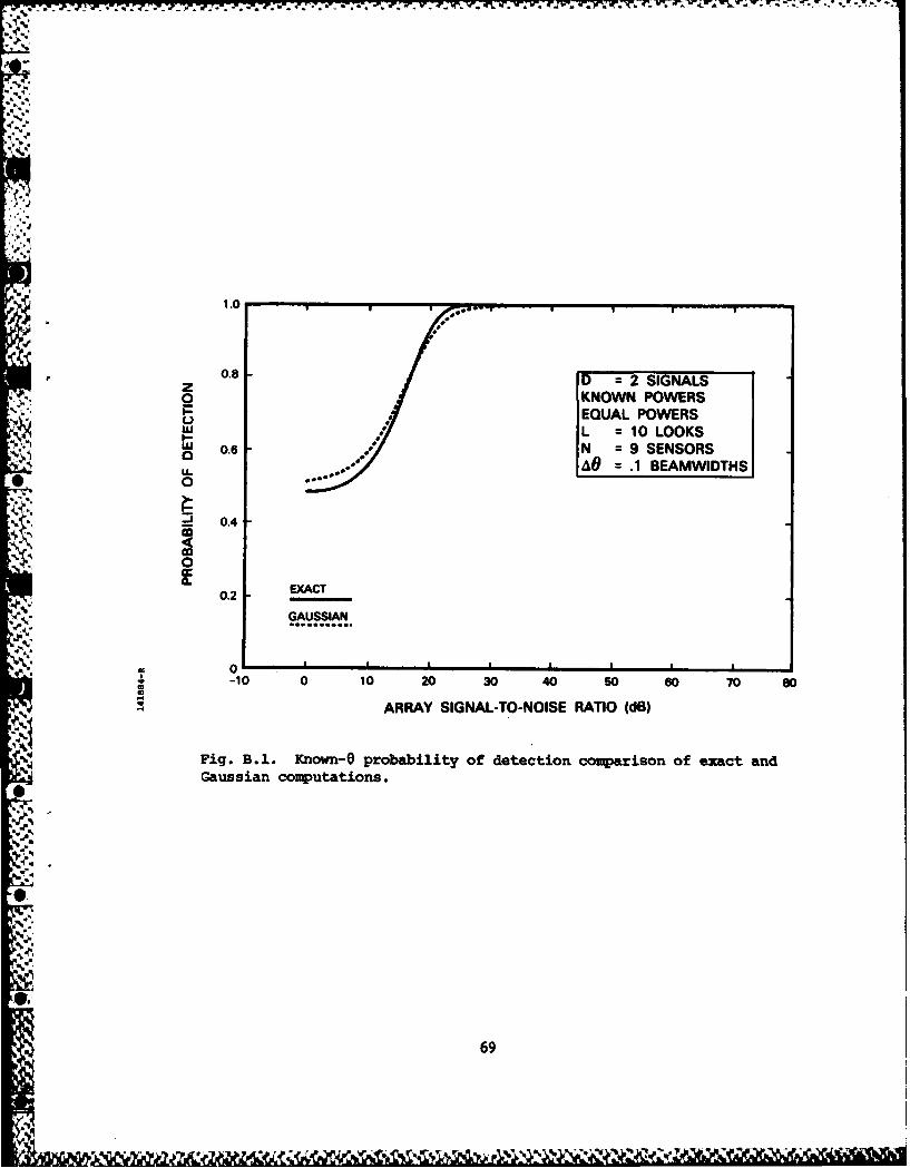
generate the solid curves in Fig. B.I.

68

-S.

°..

1.0

i 0.8 D 2 SIGNALS0 KNOWN POWERS- EQUAL POWERS"' L = 10 LOOKSLU 0.6 - N = 9 SENSORS. = .1 BEAMWDTHS

-'.

-_ 0.4

EXDC0

a. 0.2 -

GAUSSIAN.........

-10 0 10 20 30 40 50 60 70 80

ARRAY SIGNAL-TO-NOISE RATIO (dB)

Fig. B.l. Known-6 probability of detection comparison of exact andGaussian computations.

69

Unfortunately, there are numerical problems in computing the ajj'.s.

Fortunately, the pdf of t approaches Gaussian for large numbers of looks and

is reasonably close to Gaussian at the point where the exact computation

fails. Accordingly, the program optimally computes PD and PF based on a

Gaussian approximation given by

Go - 2 2" d f X - I e-(x /2a

A2 a

(1 + erf( V a ))<

where

E~) d X (s)£ - E(t) - ____o

) I + A2 + A3

and

d d2 Ys) -2

2m var(t) - ds2 -2O

I_ 2 2 2U ('I + +Y

This approximation appears as dotted curves In Fig. B.l.

70

iA.

%,A -. " .""- -"

UNCLASSIFIEDSECURITY CLASSIFICATION OF THIS PAGE (When Data Eftered)

REPORT DOCUMENTATION PAGE READ INSTRIcTIONSR DBEFORE COMPLETING FORM

1. REPORT NUMBER UT. 0 ACCESSION NO. 3. RECIPIENTS CATALOG NUMBER

ESD.TR-84-028 A 164. TITLE (and Subtitle) S. TYPE OF REPORT & PERIOD COVERED

Technical ReportPerformance of Bayes-Optimal Angle.of.Arrival Estimators

S. PERFORMING ORG. REPORT NUMBER* Technical Report 654

7. AUTHOR() I. CONTRACT OR GRANT NUMBER(s)

Fredric M. White F19628-80-C-0002,'.

V S. PERFORMING ORGANIZATION NAME AND ADDRESS 10. PROGRAM ELEMENT, PROJECT, TASK

Lincoln Laboratory, M.I.T. AREA & WORK UNIT NUMBERS

P.O. Box 73 Program Element No. 33401GL.exington, MA 02173-0073

11. CONTROLLING OFFICE NAME AND ADDRESS 12. REPORT DATE

Department of Defense 13 August 1984The Pentagon 13. NUMR OF PAGESWashington, DC 20301 78

14. MONITORING AGENCY NAME & ADDRESS (if different from Controlling Office) IS. SECURITY CLASS. (of this report)

Electronic Systems Division Unclassified

Hanscom AFB, MA 01731 Ifi. OECLASSIFICATION DOWNGRAOING SCHEDULE

16. DISTRIBUTION STATEMENT (of this Report)

Approved for public release; distribution unlimited.

17. DISTRIBUTION STATEMENT (of the abstract entered in Block 20, if different from Report)

IS. SUPPLEMENTARY NOTES

None

1. KEY WORNS (Continue on rererse side if neceuary and identify by block number)

nonlinear parameter estimation angle-of-arrival estimators Gaussian signalnonlinear filtering Monte Carlo evaluation techniques Gaussian noiseBayes-optimal estimation minimum mean-square error estimation Cramer-Rao boundspectral estimators maximum apriori probability estimation

20. ABSTRACT (Continue on rerere side if neceuary and identify by block number)

The angle-of-arrival estimation problem for waves incident upon a sensor array was examined through aMonte Carlo evaluation of the performance of the Bayes-optimal MAP (maximum aposteriori) and MMSE(minimum mean square error) estimators. The case of two independent wave emitters of known powers aswell as a multiple look, Gaussian signal in Gaussian noise statistical model were assumed. The Cramer-Rao

bound on the estimator's rms error was computed for comparison.

SI

OD FORM 1473 EDITION OF I NOV IS IS OBSOLETE UNCLASSIFIEDI Jn 73 SECURITY CLASSIFICATION OF THIS PAGE (When Owe Ente4

UNCLASSIFIEDSECURITY CLASSIFICATION OF THIS PAGE (When Data Entere)

20. ABSTRAT (camidued

The evaluation proceeded with the computation of MAP and MMSE angle estimates for 1000random samples of array outputs and the accumulation of their rms errors. The probability of de-tecting both emitters with the optimal detector was also accumulated. This was done for .1, .03,and .01 beamwidths emitter separations and a range of signal-to-noise ratios (SNRs). The accuracyof the computations was assured through a simple finite grid approximation for the estimates,with no convergence problems, and through the evaluation of statistical confidence intervals for

%' the Monte Carlo data.

The results of the evaluation indicated that the Cramer-Rao bound was achievable by both theMAP and MMSE estimators over a wide range of SNR provided a few as 10 looks had been taken.In general, the bound was achieved wherever both signals were detectable. These results were sur-prising since the bound exhibited unusual behavior; for example, in one SNR region, the boundshowed smaller rms errors for more closely-spaced emitters.

Additional results included properties of the aposteriori probability density and an analyticalcomputation of the performance of the known angles-of-arrival optimal detector.

.-

UNCLASSIFIEDSECURITY CLI.ICAION Of THIS8 PAGE. (Wr& ftm SmwO