Performance of BICM–SC and BICM–OFDM Systems with ...amirn/TCOM-08.pdfNakagami–q, and Weibull fading) and general types of noise and interference with ﬁnite moments such as

Performance of BICM–SC and BICM–OFDM Systems

with Diversity Reception in Non–Gaussian Noise and

Interference

1 Amir Nasri and Robert Schober

Department of Electrical and Computer Engineering

The University of British Columbia

2356 Main Mall, Vancouver, BC, V6T 1Z4, Canada

Phone: +604 - 822 - 3515

Fax: +604 - 822 - 5949

E-mail: {amirn, rschober}@ece.ubc.ca

In this paper, we present a general mathematical framework for performance analysis of single–

carrier (SC) and orthogonal frequency division multiplexing (OFDM) systems employing popular bit–

interleaved coded modulation (BICM) and multiple receive antennas. The proposed analysis is appli-

cable to BICM systems impaired by general types of fading (including Rayleigh, Ricean, Nakagami–m,

Nakagami–q, and Weibull fading) and general types of noise and interference with finite moments such

as additive white Gaussian noise (AWGN), additive correlated Gaussian noise, Gaussian mixture noise,

co–channel interference, narrowband interference, and ultra–wideband interference. We present an

approximate upper bound for the bit error rate (BER) and an accurate closed–form approximation for

the asymptotic BER at high signal–to–noise ratios for Viterbi decoding with the standard Euclidean

distance branch metric. Exploiting the asymptotic BER approximation we show that the diversity gain

of BICM systems only depends on the free distance of the code, the type of fading, and the number

of receive antennas but not on the type of noise. In contrast their coding gain strongly depends on

the noise moments. Our asymptotic analysis shows that as long as the standard Euclidean distance

branch metric is used for Viterbi decoding, BICM systems optimized for AWGN are also optimum for

any other type of noise and interference with finite moments.

1This work will be presented in part at the IEEE Global Telecommunications Conference (Globecom), New

Orleans, 2008.

Nasri et al.: Performance of BICM–SC and BICM–OFDM Systems 1

1 Introduction

Bit–interleaved coded modulation (BICM) is an efficient technique to extract time diversity in systems

with single–carrier (SC) modulation [1] and frequency diversity in systems employing orthogonal

frequency division multiplexing (OFDM), and has been adopted by a number of recent standards and

is also expected to play a major role in future wireless systems [2].

While wireless systems are usually optimized for additive white Gaussian noise (AWGN), in practice,

they are also subject to a multitude of other impairments such as narrowband interference (NBI)

[3], co–channel interference (CCI) [4, 5], correlated Gaussian noise and interference [6], man–made

impulsive noise [7, 8], and ultra–wideband (UWB) interference [9]–[11]. Therefore, it is of both

theoretical and practical interest to investigate how the performance of BICM–SC and BICM–OFDM

systems designed for AWGN environments is affected by non–Gaussian noise.2 We note that almost

all existing performance studies of BICM are limited to AWGN. For example, union bounds for the bit

error rate (BER) of BICM–SC were provided in [1, 12, 13] and similar expressions for BICM–OFDM

can be found in [14]. Sattlepoint approximation techniques for BICM–SC systems were introduced

in [15, 16]. The combination of BICM–OFDM and spatial diversity techniques was analyzed in

[14, 17, 18]. In contrast, only few analytical results are available for non–AWGN types of noise.

Namely, the performance of BICM–SC in Middleton’s Class A impulsive noise and of BICM–OFDM

in UWB interference was analyzed in [19] and [11], respectively.

Motivated by the lack of general performance results, in this paper, we provide a mathematical

framework for performance analysis of BICM–SC and BICM–OFDM systems employing Viterbi de-

coding with the standard Euclidean distance branch metric [1] and multiple receive antennas in fully

interleaved fading and non–AWGN environments. This framework is very general and applicable to

arbitrary linear modulation formats, all commonly used fading models, and all practically relevant

types of noise with finite moments. We first develop a general approximate upper bound on the BER

of BICM systems, which is easy to compute but offers little insight since it requires numerical inte-

gration. To overcome this problem, we derive accurate closed–form asymptotic BER approximations

for BICM–SC and BICM–OFDM systems which provide significant insight into the impact of system

parameters such as the modulation format, the free distance of the code, the type of fading, and

2In the rest of this paper, the term “noise” refers to any additive impairment of the received signal, and also

includes what is commonly referred to as “interference”.


the type of noise on performance. In particular, the asymptotic BER expressions reveal that while

the diversity gain of BICM systems is not affected by the type of noise, the coding gain depends on

certain noise moments. We note that the asymptotic performance of uncoded SC modulation has

been studied in AWGN [20, 21] and non–AWGN [22, 23] channels before. However, both the analysis

techniques and the results in [20]–[23] are not applicable to BICM.

The rest of this paper is organized as follows. In Section 2, the considered BICM–SC and BICM–

OFDM system models are introduced. The proposed upper bound and asymptotic approximation for

the BER are presented in Sections 3 and 4, respectively. Various practically relevant noise models are

discussed in Section 5. The presented analysis is verified via computer simulations in Section 6, and

conclusions are drawn in Section 7.

2 System Model

We consider BICM–SC and BICM–OFDM systems with NR receive antennas. For convenience, in

this paper, all signals and systems are represented by their complex baseband equivalents.

2.1 System Model

The BICM transmitter consists of a convolutional encoder of rate Rc, an interleaver, and a memoryless

mapper [1]. Specifically, the codeword c , [c1, c2, . . . , cmcKc] of length mcKc is generated by a

convolutional encoder and interleaved. The interleaved bits are broken up into blocks of mc bits

each, which are subsequently mapped to symbols xk from a constellation X of size |X | , M = 2mc

to form the transmit sequence x , [x1, x2, . . . , xKc] of length Kc. Assuming perfect synchronization

and demodulation, for both BICM–SC and BICM–OFDM the signal observed at the NR receive

antennas can be modeled as

rk =√

γ hk xk + nk, 1 ≤ k ≤ Kc, (1)

where hk , [hk,1 . . . hk,NR]T with E{||hk||2} = NR and nk , [nk,1 . . . nk,NR

]T with E{||nk||2} =

NR contain the fading gains hk,l and the noise variables nk,l, 1 ≤ l ≤ NR, respectively, and γ denotes

the signal–to–noise ratio (SNR) per receive antenna.3 As customary in the literature, cf. e.g. [1, 13,

3In this paper, [·]T , (·)H , ℜ{·}, || · ||, det(·), and Ex{·} denote transposition, Hermitian transposition, the real

part of a complex number, the L2–norm of a vector, the determinant of a matrix, and statistical expectation with


17], for our performance analysis we assume perfect interleaving, which means that hk and nk can

be modeled as independent, identically distributed (i.i.d.) random vectors and only their first order

probability density functions (pdfs) are relevant. Thus, to simplify our notation, in the following, we

will drop the time/frequency index k wherever possible. We discuss the assumptions necessary for

the validity of the i.i.d. assumption more in detail below.

BICM–SC: For BICM–SC we assume transmission over a flat fading channel and coding over

B frames of N data symbols, i.e., Kc = NB. The channel is time–variant within one frame and

changes independently from frame to frame (e.g. due to frequency hopping). For sufficiently large N

and/or B assuming that the time–domain fading vectors hk are i.i.d. is justified [1].

BICM–OFDM: We consider a BICM–OFDM system with N sub–carriers where one codeword

spans B OFDM symbols, i.e., Kc = BN . We assume that the length of the OFDM cyclic prefix

exceeds the length of the channel impulse response and that the channel changes independently

from OFDM symbol to OFDM symbol. Thus, modeling the frequency–domain channel gains hk as

i.i.d. vectors implies that the channel is severely frequency selective and/or B is sufficiently large.

Practical BICM–SC and BICM–OFDM systems that employ interleaving and coding over B > 1

frequency–hopped frames include the GSM/EDGE mobile communication system (N = 116/N =

348, B = 8) and the ECMA multi–band OFDM (MB–OFDM) UWB system (N = 128, B = 3;

future versions of the standard may use up to B = 15) [9], respectively.

2.2 Fading and Noise Model

Fading Model: The fading gains can be expressed as hl , alejΘl, where al and Θl are mutually

independent random variables (RVs). Specifically, Θl is uniformly distributed in [−π, π) and al is a

positive real RV characterized by its distribution pa,l(al) or equivalently by its moment generating

function (MGF) Φa,l(s) , E{e−sal}. Correlated fading can be modeled via the joint pdf pa(a) or

the joint MGF Φa(s) , E{e−PNR

l=1slal}, s , [s1 . . . sNR

]T , of the elements of a , [a1 . . . aNR]T ,

cf. e.g. [24]–[26]. For the asymptotic analysis in Section 4, we require the fading channel to be

respect to x, respectively. Moreover, IM and 0M are the M ×M identity matrix and the all–zero column vector

of length M , respectively. Furthermore, we use the notation u ⊜ v to indicate that u and v are asymptotically

equivalent, and a function f(x) is o(g(x)) if limx→0 f(x)/g(x) = 0.


asymptotically spatially i.i.d., i.e., for a → 0NRthe joint pdf can be expressed as

pa(a) ⊜

NR∏

l=1

pa(al), (2)

where

pa(a) = 2αca2αd−1 + o(a2αd−1) (3)

with fading distribution dependent constants αc and αd. Eq. (2) is obvious for i.i.d. and independent,

non–identically distributed (i.n.d.) fading [20]–[22], and we prove its validity for the most popular

correlated fading models (Rayleigh, Ricean, and Nakagami–m) in Appendix A. For these correlated

fading models and for independent Nakagami–q and Weibull fading, the fading pdf pa,l(al) and

parameters αc and αd are specified in Table 1.

Noise Model: The proposed analysis is very general and applicable to all types of noise for which

all joint moments of the elements of n exist. This is a mild condition which is met by most practically

relevant types of noise and interference, see Section 5 for several examples. An exception is α–stable

noise, which is sometimes used to model impulsive noise [27], as the higher order moments of α–

stable noise do not exist. Note that our analysis is applicable to other types of impulsive noise such

as Middleton’s Class–A model and ǫ–mixture noise.

3 Approximate Upper Bound for BER

In this section, we present an approximate upper bound for the BER of BICM systems operating in

non–AWGN environments.

3.1 MGF of Metric Difference

We assume Viterbi decoding with the standard Euclidean (ED) branch metric [1]

λi , minx∈X i

b

{

||r −√γ hx||2

}

(4)

for bit i, 1 ≤ i ≤ mc, of symbol x. Here, X ib denotes the subset of all symbols in constellation X

whose label has value b ∈ {0, 1} in position i. In AWGN, the ED branch metric λi performs close to

optimum at sufficiently high SNR [1]. In non–Gaussian noise, significant performance gains could be

achieved with optimum maximum–likelihood (ML) decoding, which, however, requires knowledge of


the noise pdf. Since this knowledge is typically not available at the receiver, in most practical systems,

the ED branch metric is also used in the presence of non–Gaussian impairments. For derivation of

the proposed upper bound it is convenient to first calculate the MGF of the metric difference

∆(x, z) , ||r −√γ h z||2 − ||r −√

γ hx||2 = d2xz γ||h||2 − 2 dxz

√γ ℜ{hHn}, (5)

where x denotes the transmitted symbol and z is the nearest neighbor of x in X ib

with b being the

bit complement of b, and x − z , dxzejΘd with ED dxz > 0. Since we assume the phases Θl of hl

to be uniformly distributed, in (5), we have absorbed ejΘd in h without loss of generality. Based on

(5) the MGF Φ∆(x,z)(s) , Eh,n{e−s∆(x,z)} of ∆(x, z) can be expressed as

Φ∆(x,z)(s) = Eh{e−d2xz γ||h||2 s En{e2 dxz

√γ ℜ{hH

n} s}} = Ea{e−d2xz γ||a||2 s Φn(−2 dxz

√γ as)}, (6)

where n , [e−jΘ1n1 . . . e−jΘNRnNR]T and Φn(s) , En{e−sT ℜ{n}} is the MGF of n. If the phases

of the noise components nl, 1 ≤ l ≤ NR, are mutually independent and uniformly distributed in

[−π, π), Φn(s) = Φn(s) , En{e−sT ℜ{n}} is valid and Φn(s) in (6) can be replaced by Φn(s).

Further simplifications are possible if both the phases and the amplitudes of nl, 1 ≤ l ≤ NR, are

mutually independent. In this case, we can express Φn(s) as

Φn(s) =

NR∏

l=1

Φnl(slℜ{nl}), (7)

where only the scalar MGFs Φnl(s) , Enl

{e−sℜ{nl}} of the elements nl , e−jΘlnl of n are required.

If the phases of the nl, 1 ≤ l ≤ NR, are uniformly distributed in [−π, π), Φnl(s) = Φnl

(s) ,

Enl{e−sℜ{nl}} is valid, i.e., only the scalar MGFs of the noise components are required.

The scalar MGFs Φnl(s) of several practically relevant types of noise are collected in Table 2,

cf. Section 5. If Φn(s) cannot be calculated in closed form, it can be computed by numerical

integration even if Φn(s) = Φn(s) is not valid (i.e., if the phases of nl, 1 ≤ l ≤ NR, are not

mutually independent and/or are not uniformly distributed in [−π, π)). However, even if closed–form

expressions for the MGF are available, calculation of Φ∆(x,z)(s) in closed form is usually not possible,

and evaluation of (6) entails NR numerical integrals.


3.2 Approximate Upper Bound

Assuming a convolutional code of rate Rc = kc/nc (kc and nc are integers) the union bound for the

BER of BICM is given by [1]

Pb ≤1

kc

∞∑

d = df

wc(d) P (c, c), (8)

where c and c are two distinct code sequences with Hamming distance d that differ only in l ≥ 1

consecutive trellis states, wc(d) denotes the total input weight of error events at Hamming distance

d, and df is the free distance of the code. P (c, c) is the pairwise error probability (PEP), i.e., the

probability that the decoder chooses code sequence c when code sequence c 6= c is transmitted.

Invoking the expurgated bound from [1], the PEP can be expressed as

P (c, c) =1

2πj

c+j∞∫

c−j∞

1

mc2mc

mc∑

i=1

1∑

b=0

∑

x∈X ib

Φ∆(x,z)(s)

d

ds

s, (9)

where c is a small positive constant that lies in the region of convergence of the integrand. The

integral in (9) can be efficiently evaluated numerically using a Gauss–Chebyshev quadrature rule,

cf. [28]. Eqs. (8) and (9) constitute an approximate upper bound on the BER and are generalizations

of similar bounds in [1, 17] for AWGN to arbitrary types of noise (and interference). We cannot prove

that (8) with (9) is a true upper bound since, as has been pointed out in [12], the proof provided in

[1] for the expurgated bound is not correct. Nevertheless, our results in Section 6 do suggest that

(8) with (9) is an asymptotically tight upper bound if Gray labeling is applied. We note that all our

results can be extended to the revised expurgated bounds presented in [12].

4 Asymptotic Analysis

In this section, we analyze the asymptotic behavior of the upper bound in (8) for high SNR, i.e.,

γ → ∞. For this purpose, it is convenient to consider the conditional PEP

P (c, c |n) =1

2πj

c+j∞∫

c−j∞

Φ(s|n)ds

s, (10)

Φ(s|n) =

1

mc2mc

mc∑

i=1

1∑

b=0

∑

x∈X ib

Φ∆(x,z)(s|n)

d

, (11)


where Φ∆(x,z)(s|n) = Ea,Θ{e−s∆(x,z)} with channel phase vector Θ , [Θ1 . . . ΘNR]T . The condi-

tional PEP in (10) is given by the sum of the residues of Φ(s|n)/s at poles lying in the left hand

side (LHS) of the complex s–plain (including the imaginary axis) [28]. In order to investigate the

singularities of Φ(s|n)/s, we derive the Laurent series representation of Φ(s|n) around s = 0 for the

asymptotic case of γ → ∞ in the following subsection.

4.1 Laurent Series Expansion of Φ(s|n)

For γ → ∞ errors only occur for small channel gains, i.e., for a → 0NR, see also [21]. Exploiting

the fact that the elements of a and Θ are asymptotically i.i.d. for γ → ∞, cf. Section 2.2, we can

rewrite Φ∆(x,z)(s|n) as

Φ∆(x,z)(s|n) ⊜

NR∏

l=1

Φ∆(x,z)(s|nl), (12)

where Φ∆(x,z)(s|nl) , Eal,Θl{ e−sγ d2

xz |al|2 e2√

γdxz alℜ{nl} s}. Using the Taylor series expansion ex =∑∞

i=0 xi/i!, the integral∫∞0

xµ−1e−px2

dx = pµ/2Γ(µ/2) [29, 3.462], and (3), Φ∆(x,z)(s|nl) can be

expressed as

Φ∆(x,z)(s|nl) = Eal,Θl

{

e−sγ d2xz |al|2

∞∑

i=0

(2√

γdxz alℜ{nl} s)i/i!

}

=αc

(γd2xzs)

αd

∞∑

i=0

2iΓ(αd + i/2)EΘl{ℜ{nl}i}si/2 + o

(

γ−αd)

. (13)

Using EΘl{ℜ{nl}i} = i/2+1/2√

πΓ(i/2+1)|nl|i, i even, and EΘl

{ℜ{nl}i} = 0, i odd, in (13) leads to

Φ∆(x,z)(s|nl) =αc

(γd2xzs)

αd

∞∑

i=0

βi|nl|2isi + o(

γ−αd)

, (14)

where βi is defined as

βi ,22iΓ(αd + i)Γ(i + 1/2)

(2i)!Γ(i + 1)=

Γ(αd + i)

(i!)2. (15)

The asymptotic Laurent series expansion of Φ(s|n) is obtained from (11), (12), and (14) as

Φ(s|n) = X(α, NR, d) αNRdc (γs)−αdNRd

(

NR∏

l=1

zl(s)

)d

+ o(

γ−αdNRd)

(16)

with zl(s) ,∑∞

i=0 βi|nl|2isi and modulation dependent constant

X(αd, NR, d) ,

1

mc2mc

mc∑

i=1

1∑

b=0

∑

x∈X ib

1

(d2xz)

αdNR

d

. (17)


In the next subsection, we will use (16) to calculate a closed–form expression for the asymptotic BER.

4.2 Approximation for Asymptotic BER

As mentioned before, the conditional PEP (10) is given by the sum of the residues of Φ(s|n)/s in the

LHS of the complex s–plain. Using d’Alembert’s convergence test [29, 0.222] it is easy to show that

zl(s) is convergent for all s. Thus, (∏NR

l=1 zl(s))d is also convergent for all s. Consequently, the first

term on the right hand side (RHS) of (16), which dominates for high SNR, is convergent for s 6= 0,

i.e., for high SNR the only singularity of Φ(s|n)/s is at s = 0. Thus, the asymptotic conditional

PEP is given by the residue of Φ(s|n)/s at s = 0 or equivalently by the coefficient associated with

s0 in the series expansion of the first term on the RHS of (16). Assuming αdNRd is an integer this

leads to

P (c, c |n) = X(αd, NR, d) αNRdc γ−αdNRd

∑

i1+···+id=αdNRd

d∏

k=1

∑

j1+···+jNR=ik

βj1|n1|2j1 · · ·βjNR|nNR

|2jNR

+o(

γ−αdNRd)

. (18)

Based on (8) and (18) a closed–form approximation for the asymptotic unconditional BER Pb ⊜wc(df )

kc

E{P (c, c |n)} can be obtained as

Pb ⊜wc(df)

kc

αNRdfc X(αd, NR, df) M(αd, NR, df) γ−αdNRdf , (19)

where

M(αd, NR, d) =∑

i1+···+id=αdNRd

d∏

k=1

∑

j1+···+jNR=ik

βj1 · · ·βjNRMn(j1, . . . , jNR

), (20)

with the joint noise moments

Mn(j1, . . . , jNR) , En

{

|n1|2j1 . . . |nNR|2jNR

}

. (21)

In arriving at (19)–(21) we have used the assumptions that (a) the first term in the summation in (8) is

asymptotically dominant, (b) the union bound is an accurate approximation for the BER at high SNR,

(c) the noise vectors n are i.i.d., and (d) all joint moments of the elements of n exist. Assumption

(d) is necessary since the terms absorbed in o(γ−αdNRd) in (18), contain sums of products of elements

of n, cf. (13), which have been neglected in (19). At what finite SNR the approximate upper bound

(10) and the true BER approach the asymptotic BER depends on how fast the terms neglected in


(19) become negligible compared to the terms considered as the SNR increases. Generally, the SNR

values at which the asymptotic BER is approached increase with increasing αdNRdf and increasing

w(df + 1)/w(df) since higher SNRs are necessary for the term w(df)γ−αdNRdf considered in (19)

to dominate the largest term w(df + 1)γ−αdNRdf−1 absorbed in o(γ−αdNRd). Thus, we expect the

asymptotic BER to converge faster to the true BER for codes with smaller free distance df and

smaller relative weight w(df + 1)/w(df), cf. Fig. 3. Furthermore, depending on the properties of the

noise, evaluation of Mn(j1, . . . , jNR) may be cumbersome. However, for two important special cases

significant simplifications are possible.

Case 1 (spatially i.i.d. noise): If the components of n are independent, (20) simplifies to

M(αd, NR, d) =∑

j1+···+jNRd=αdNRd

βj1Mn(j1) . . . βjNRdMn(jNRd) (22)

with scalar noise moments Mn(j) , E{|nl|2j}, which are independent of l.

Case 2 (αd = 1): If αd = 1, which is true for example for (possibly spatially correlated) Rayleigh,

Ricean, and Nakagami–q fading, (20) simplifies to

M(1, NR, d) =1

(NRd)!

∑

i1+···+id=NRd

(

NRd

i1, . . . , id

)

Mn(i1) . . .Mn(id) (23)

with vector noise moments Mn(i) , E{||n||2i}.Closed–form expressions for the moments Mn(j) and Mn(i) of several important types of noise

are provided in Tables 2 and 3, respectively, cf. Section 5.

In the remainder of this section, we discuss the implications of the asymptotic BER (19) for

system design and consider the special cases of AWGN and uncoded transmission, respectively.

4.3 Diversity Gain, Coding Gain, and Design Guidelines

To get more insight, it is convenient to express the asymptotic BER as Pb ⊜ (Gcγ)−Gd [21], where Gd

and Gc denote the diversity gain (i.e., the asymptotic slope of the BER curve on a double logarithmic

scale) and the coding gain (i.e., a relative horizontal shift of the BER curve), respectively. Considering

the asymptotic BER in (19), we obtain

Gd = αdNRdf (24)

Gc [dB] = −10

αdlog10 αc −

10

Gdlog10

(

wc(df)X(αd, NR, df)

kc

)

− 10

Gdlog10 M(αd, NR, df) (25)


From (24) we observe that the diversity gain of BICM is independent of the type of noise. The coding

gain in (25) consists of three terms, where the first, the second, and the third term depend on the

fading channel, the modulation scheme and the code, and the type of noise, respectively. The primary

goal of BICM design is to maximize df for a given decoding complexity in order to maximize Gd (and

to minimize the asymptotic BER). Gray labelings (yielding smaller X(αd, NR, df) than non–Gray

labelings) and codes with small wc(df) are advantageous for maximizing the second, modulation and

coding dependent term in (25). Once df is fixed, the last term in (25) cannot be further influenced

through system design making the BICM design guidelines effectively indepenent of the type of noise

in the system. Thus, our results show that BICM systems optimized based on the guidelines provided

in [1] for systems operating in fading and AWGN are also optimum for non–AWGN environments as

long as the standard ED branch metric is used for Viterbi decoding.

4.4 Special Case I: AWGN

Although the main focus of this paper is non–AWGN, the presented results are also valid for AWGN.

We note that although the AWGN case was covered extensively in the literature, e.g. [1, 13, 17],

our results are still more general than existing results as they allow for spatially correlated fading and

more general fading models. For example, for Ricean fading (αd = 1) we obtain from (22) with the

help of (15) and Table 2 M(1, NR, d) =(

2NRdf−1NRdf

)

. Thus, with (19) and Table 1 we get

Pb ⊜

(

2NRdf − 1

NRdf

)

(

wc(df) exp(

−µHh C−1

hhµh

)

kc det(Chh)

)df

X(1, NR, df) γ−NRdf , (26)

which is a new result. For NR = 1, we may rewrite (26) as Pb ⊜(

2df−1df

)wc(df )

kc[(1 + K)e−K ]df X(1,

1, df)γ−df with Ricean factor K , |µh|2/σ2

h, where µh and σ2h denote the mean and the variance

of h1. In contrast, for Ricean fading with NR = 1 the Chernoff bound was used in [1] and [17] to

investigate the asymptotic behavior of BICM–SC and BICM–OFDM, respectively, since “a closed–

form expression for the PEP for arbitrary K is missing” [1]. Comparing our result with the asymptotic

Chernoff bound [1, Eq. (62)] shows that the Chernoff bound is by a factor of 4df /(

2df−1df

)

> 1 larger

than the asymptotic BER, i.e., for df = 3 and df = 6 the Chernoff bound is horizontally shifted by

2.7 dB and 1.6 dB compared to the asymptotic BER, respectively. Furthermore, using the Stirling

approximation we obtain for the difference between asymptotic Chernoff bound and asymptotic BER

4df /(

2df−1df

)

→ 2√

πdf for df ≫ 1, which agrees with the result obtained in [16] for Rayleigh fading.


4.5 Special Case II: Uncoded Transmission

While BICM is the main focus of this paper, based on (19) it is also possible to compute the asymptotic

BER of uncoded transmission with maximum–ratio combining (MRC) at the receiver. In this case,

df = 1, kc = 1, and wc(1) = 1 are valid. Furthermore, assuming a regular signal constellation such

as M–ary quadrature amplitude modulation (M–QAM) or M–ary phase shift keying (M–PSK), it is

easy to see that X(αd, NR, 1) = Nmin/(mcd2αdNR

min ), where Nmin and dmin are the average number of

minimum distance neighbors and the minimum distance of X , respectively. Therefore, the asymptotic

BER of uncoded transmission with MRC can be expressed as

Pb ⊜Nminα

NRc

mcd2αdNR

min

M(αd, NR, 1) γ−αdNR , (27)

where M(αd, NR, 1) =∑

j1+···+jNR=αdNR

βj1 · · ·βjNRMn(j1, . . . , jNR

), which can be further sim-

plified for αd = 1 and spatially i.i.d. noise, cf. Section 4.2. In particular, for αd = 1 we obtain

M(1, NR, 1) = Mn(NR)/NR!, cf. (23), and it can be shown that for Rayleigh and Ricean fading (for

both of which αd = 1 holds) (27) is identical to [23, Eqs. (12), (16)]. However, (27) is more general

than the results in [23] since it is not limited to Rayleigh and Ricean fading and is also applicable to

e.g. Nakagami–m, Nakagami–q, and Weibull fading.

5 Calculation of the Noise Moments and MGFs

In this section, we discuss several practically relevant types of noise and compute the corresponding

MGFs Φn(s) and moments Mn(j1, . . . , jNR) required for evaluation of the upper bound in Section 3

and the asymptotic BER in Section 4, respectively. We note that for spatially i.i.d. noise only the scalar

MGFs Φn(s) and the scalar moments Mn(i) have to be computed for evaluation of the upper bound

and the asymptotic BER, respectively, cf. (7), (22), Table 2. Furthermore, for most types of spatially

dependent noise, it is difficult to find closed–form expressions for the joint MGF Φn(s) and the joint

moments Mn(j1, . . . , jM ), since the phases of the elements of n are not independent. Therefore,

unless stated otherwise, we concentrate in case of spatially dependent noise on the important special

cases αd = 1 (with arbitrary NR) and NR = 1 (with arbitrary αd), where only the vector moments

Mn(i) and the scalar moments Mn(i) of the noise are required, respectively.


5.1 Noise Models for BICM–SC

In this section, we consider several time–domain noise models typical for BICM–SC systems. In

particular, we consider spatially independent Gaussian–mixture noise (SI–GMN) and three different

types of spatially dependent noise (spatially dependent (SD) GMN, additive correlated Gaussian noise

(ACGN), and asynchronous co–channel interference (CCI)).

SI–GMN: GMN is often used to model the combined effect of Gaussian background noise and

man–made or impulsive noise, cf. e.g. [7, 8, 19]. If the phenomenon causing the impulsive behavior

affects the antennas independently, the GMN is spatially i.i.d. [30] and nl is distributed according to

[8]

pn(nl) =

I∑

i=1

ci

πσ2i

exp

(

−|nl|2σ2

i

)

, 1 ≤ l ≤ NR, (28)

where ci > 0 and σ2i > 0 are parameters, and

∑Ii=1 ci σ

2i = 1. Two popular special cases of Gaussian

mixture noise are Middleton’s Class–A noise [8] and ǫ–mixture noise. For ǫ–mixture noise I = 2,

c1 = 1 − ǫ, c2 = ǫ, σ21 = σ2

g , and σ22 = κσ2

g , where ǫ is the fraction of time when the impulsive noise

is present, κ is the ratio of the variances of the Gaussian background noise and the impulsive noise,

and σ2g = 1/(1 − ǫ + κǫ) = 1. The scalar MGF Φn(s) and the scalar moments Mn(i) for SI–GMN

are given in Table 2.

SD–GMN: SD–GMN is an appropriate model for impulsive noise if all antennas are affected

simultaneously by the phenomenon causing the impulsive behavior. The joint pdf for SD–GMN n is

given by [30]

pn(n) =

I∑

i=1

ci

πNRσ2NR

i

exp

(

−||n||2σ2

i

)

, (29)

where ci and σ2i are defined similarly as for SI–GMN. Since the phases of the elements of n are

independent random variables, the joint MGF Φn(s) can be calculated to

Φn(s) =

I∑

i=1

ci exp

(

σ2i

4

NR∑

l=1

s2l

)

. (30)

Furthermore, in this particular case, a closed–form expression for the joint moment Mn(j1, . . . , jNR),

cf. (21), can be obtained as

Mn(j1, . . . , jNR) = j1! · · · jNR

!I∑

i=1

ciσ2(j1+···+jNR

)

i . (31)

The vector moments Mn(i) are provided in Table 3.


ACGN: In BICM–SC systems, correlated Gaussian noise n may be caused by narrowly spaced

receive antennas [6]. Correlated Gaussian interference n = hb + n is caused by a synchronous

co–channel interferer transmitting i.i.d. PSK symbols b over a spatially correlated Rayleigh fading

channel with gains h and AWGN n. In both cases n is fully characterized by its covariance matrix

Cnn , E{nnH}, and the corresponding vector moments Mn(i) are given in Table 3, where λl,

1 ≤ l ≤ NR, denotes the eigenvalues of Cnn.

Asynchronous CCI: Another common type of non–AWGN impairment in BICM–SC systems is

asynchronous CCI [4, 5]. We consider coding over B different hopping frequencies and assume

that at hopping frequency µ, 1 ≤ µ ≤ B, in addition to AWGN nµ, there are Iµ Rayleigh faded

asynchronous CCI signals leading to time–domain noise

nµ =

Iµ∑

i=1

hµ[i]ku∑

l=kl

gi,µ[l]bi,µ[l] + nµ, (32)

where hµ[i] and bi,µ[l] ∈ Mi,µ ( Mi,µ: Mi,µ–ary symbol alphabet) denote the temporally i.i.d. zero–

mean Gaussian random channel vector and the i.i.d. symbols of the ith interferer at the µth hopping

frequency, respectively. Furthermore, gi,µ[l] , gi,µ(lT + τi,µ), where gi,µ(t), T , and τi,µ are the

effective pulse shape, the symbol duration, and the time offset of the ith interferer at the µth

hopping frequency, respectively. We assume that gi,µ(lT + τi,µ) ≈ 0 for i < kl and i > ku, denote

the set of all possible values of ξi,µ ,∑ku

l=klgi,µ[l]bi,µ[l] by Si,µ, and define Sµ , S1,µ × . . . × SIµ,µ.

If Iµ = 0, we formally set Sµ = {0} with |Sµ| = 1. With these definitions, the pdf of nµ can be

expressed as

pn(n) =B∑

µ=1

∑

Sµ

cµ,Sµ

πNR det(CSµ)

exp(

−nHC−1Sµ

n)

, (33)

where cµ,Sµ, 1/(|Sµ|B) and CSµ

,∑Iµ

i=1 |ξi,µ|2E{hµ[i]hH

µ [i]} + σ2nINR

(σ2n: variance of elements

of nµ). Eq. (33) shows that CCI in BICM–SC systems can be interpreted as correlated Gaussian

mixture noise. For future reference we denote the ratio of the total CCI variance and the total AWGN

variance by κ, cf. Section 6. The scalar moments Mn(i) (valid for NR = 1) and vector moments

Mn(i) of asynchronous CCI are given in Tables 2 and 3, respectively, where we have replaced CSµ

by σ2Sµ

for NR = 1 in Table 2, and in Table 3, λl,Sµ, 1 ≤ l ≤ NR, are the eigenvalues of CSµ

.


5.2 Noise Models for BICM–OFDM

Now, we turn our attention to several frequency–domain noise models relevant to BICM–OFDM

systems. In particular, we consider SI–GMN and two types of spatially dependent noise (SD–GMN

and narrowband interference (NBI)).

SI–GMN: Taking into account that in OFDM systems time domain and frequency domain are

linked via the discrete Fourier transform (DFT), it can be shown that time–domain SI–GMN (28)

results in frequency–domain noise with pdf

pn(nl) =∑

k1+···+kI=N

ck1,...,kI

πσ2k1,...,kI

exp

(

− |nl|2σ2

k1,...,kI

)

, 1 ≤ l ≤ NR, (34)

which is again an SI–GMN model with parameters ck1,...,kI,(

Nk1,...,kI

)

ck1

1 · · · ckI

I and σ2k1,...,kI

,

(k1σ21 + · · · + kIσ

2I )/N . We note that the spectral i.i.d. asumption for nl is justified only if the

interleaver spans several OFDM symbols, i.e., B ≫ 1, since the noise after DFT in one OFDM

symbol will be spectrally dependent. The scalar MGF Φn(s) and the scalar moments Mn(i) for

SI–GMN are provided in Table 2.

SD–GMN: The DFT operation at the receiver transforms the noise pdf (29) into

pn(n) =∑

k1+···+kI=N

ck1,...,kI

πNRσ2NR

k1,...,kI

exp

(

− ||n||2σ2

k1,...,kI

)

, (35)

where the same definition is used for ck1,...,kIand σ2

k1,...,kIas for SI–GMN, cf. (34). Since, similar

to the BICM–SC case, the phases of the elements of n are independent random variables, the joint

MGF can be obtained as

Φn(s) =∑

k1+···+kI=N

ck1,...,kIexp

(

σ2k1,...,kI

4

NR∑

l=1

s2l

)

. (36)

The corresponding joint moment is given by

Mn(j1, . . . , jNR) = j1! · · · jNR

!∑

k1+···+kI=N

ck1,...,kIσ

2(j1+···+jNR)

k1,...,kI. (37)

The vector moments Mn(i) for SD–GMN are provided in Table 3.

NBI: We consider a BICM–OFDM system with coding over B different hopping frequencies. At

hopping frequency µ, 1 ≤ µ ≤ B, the received frequency–domain signal is impaired by AWGN nk,µ

and Iµ Rayleigh faded PSK NBI signals. The corresponding frequency–domain noise model is

nk,µ =

Iµ∑

i=1

gk,µ[i]bµ[i]hk,µ[i] + nk,µ, 1 ≤ k ≤ N, (38)


where bµ[i] is the PSK symbol of the ith interferer at the µth hopping frequency affecting the set Nµ,i

of sub–carriers via gk,µ[i] , exp[−jπ(N −1)(k+fµ,i/∆fs)/N +φµ,i] sin[π(k+fµ,i/∆fs)]/ sin[π(k+

fµ,i/∆fs)/N ] [3]. Here, fµ,i and φµ,i denote the frequency and phase of the ith interferer at hopping

frequency µ relative to the user, respectively, and ∆fs is the OFDM sub–carrier spacing. Since

we consider NBI, the same interference fading vector hk,µ[i] (modeled as spatially correlated zero–

mean Gaussian random vector) affects all sub–carriers in Nµ,i. For fµ,i = ν∆f , the NBI affects

only sub–carrier ν, i.e., Nµ,i = ν, while, in theory, for fµ,i 6= ν∆f the NBI affects all sub–carriers.

However, gk,µ[i] decays quickly and we limit Nµ,i such that |gk,µ[i]| ≈ 0 for k 6∈ Nµ,i. Finally, we

assume that no sub–carrier is affected by two narrowband interferers at a given hopping frequency,

i.e., Nµ,i1 ∩ Nµ,i2 = ∅, i1 6= i2. The pdf for this general interference scenario is given by

pn(n) =

B∑

µ=1

Iµ∑

i=1

∑

k∈Nµ,i

c0

πNR det(Cµ,i,k)exp

(

−nHC−1µ,i,kn

)

+c1

πNRσ2NR

n

exp

(

−||n||2σ2

n

)

, (39)

where σ2n denotes the variance of the elements of the AWGN n, c0 , 1/(BN), c1 , 1−∑B

µ=1

∑Iµ

i=1

|Nµ,i|/(BN), Cµ,i,k , |gk,µ[i]|2Cµ,i+σ2nINR

, and Cµ,i , E{hk,µ[i](hk,µ[i])H}. Eq. (39) shows that,

similar to CCI in BICM–SC systems, NBI in BICM–OFDM systems can be interpreted as correlated

Gaussian mixture noise. We denote the ratio of the total NBI variance and the AWGN variance by

κ, cf. Section 6. The corresponding moments Mn(i) and Mn(i) are provided in Tables 2 and 3,

respectively, where we have replaced Cµ,i,k by σ2µ,i,k for NR = 1 in Table 2, and in Table 3, λl,µ,i,k,

1 ≤ l ≤ NR, are the eigenvalues of Cµ,i,k.

5.3 Monte–Carlo Method

For complicated types of noise such as UWB interference, it may be difficult to calculate the moments

Mn(i), Mn(i), and Mn(j1, . . . , jNR) in closed form. In this case, these moments may be obtained by

Monte–Carlo simulation of (21), (22), or (23) and subsequently be used in (19) for calculation of the

asymptotic BER. We note that this semi–analytical approach is much faster than a full simulation

since the moments are independent from the SNR γ and have to be computed only once.


6 Numerical and Simulation Results

In this section, we verify our derivations in Sections 3–5 with computer simulations and employ the

presented theoretical framework to study the performance of BICM in non–AWGN environments.

For the simulations, we consider both idealized channels with temporally i.i.d. channel and noise

vectors, and non–ideal channels generated based on the models presented in Sections 2.1 and 5.

In the non–ideal case, for BICM–SC we assume a frame size of N = 972 and a normalized fading

bandwidth BfT of 0.007, which are typical values for the DAMPS mobile communication system

[4]. For BICM–OFDM we consider systems with N = 64 and N = 128 sub–carriers transmitting

over channels with L = 10 and L = 20 i.i.d. impulse response coefficients. For all simulations

shown, a pseudo–random interleaver was employed. Throughout this section we adopt the standard

convolutional code with rate Rc = 1/2 and generator polynomials [133, 171] (octal representation).

Higher code rates are obtained via puncturing and, unless specified otherwise, 4–PSK modulation

and NR = 1 receive antennas are used. The parameters of the adopted noise models are specified in

the respective captions of Figs. 1–7.

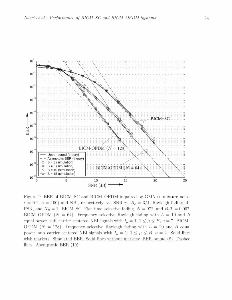
In Fig. 1, we show simulation results for BICM–SC and BICM–OFDM impaired by GMN and

NBI, respectively. In both cases, coding (Rc = 3/4) and interleaving is performed over different

numbers of frames B. Besides the simulation results we also show the approximate upper bound

and the asymptotic BER derived in Sections 3 and 4, respectively. For high enough SNR and BICM–

OFDM with N = 128 and the severely frequency–selective channel with L = 20 the analytical

results are accurate even for B = 3. In contrast, for BICM–SC and BICM–OFDM with N = 64 and

L = 10 the interleaver is not able to generate i.i.d. channels for small B which leads to performance

degradation and the corresponding simulated BER exceeds the upper bound (which was derived

assuming i.i.d. channels). However, as B increases, the simulation results approach the upper bound

and the asymptotic BER also in these cases for high SNR. Note that for non–delay critical applications,

such as data transmission, large B can be afforded.

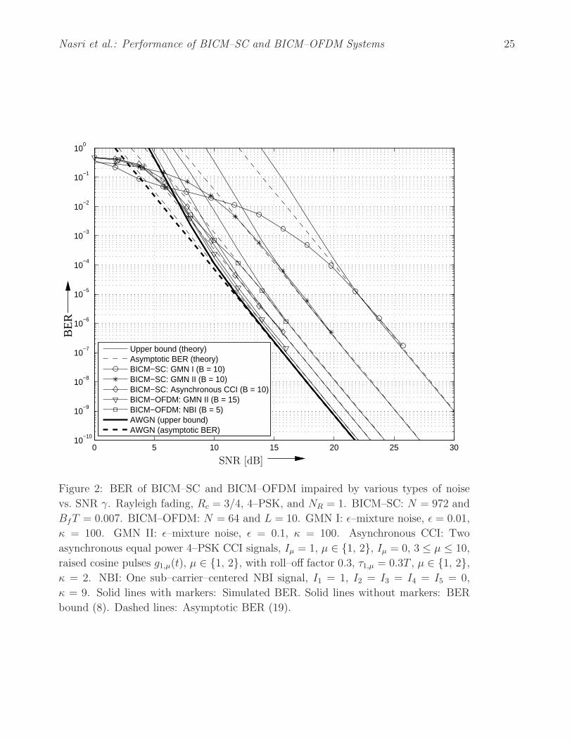
In Fig. 2, we show the BER of BICM–SC and BICM–OFDM (N = 64) for Rayleigh fading

and various different noise and interference scenarios. Fig. 2 shows that the simulated BERs (solid

lines with markers), which were generated with non–ideal channels and for different B, approach

the approximate upper bound (solid lines without markers) and the asymptotic BER (dashed lines)

for high SNR. In particular, for the BER region of BER < 10−5, which is difficult to simulate, the


proposed analytical results are accurate approximations for the true BER. The simulated BER exceeds

the upper bound again because of the non–ideal channel. In accordance with our findings in Section

4.3, Fig. 2 shows that for high SNR all BER curves are parallel, i.e., all considered types of noise lead

to the same diversity gain of Gd = df = 5. Nevertheless, there are large performance differences

between different types of noise because of the different coding gains Gc. Fig. 2 confirms that

OFDM is far more robust to GMN than SC if BICM is used in both cases. For GMN II BICM–OFDM

outperforms BICM–SC by 5 dB at high SNR and approaches the performance in AWGN. This is an

interesting result, since a previous comparison in [19] had shown that BICM–SC is more robust to

GMN than uncoded OFDM. Note, however, that for BICM–OFDM a relative large B is necessary

to make the GMN approximately spectrally independent, whereas for BICM–SC GMN is temporally

independent even for B = 1, cf. Section 5.

In the remaining figures, we assume ideal channels where both fading and noise are temporally or

spectrally i.i.d.

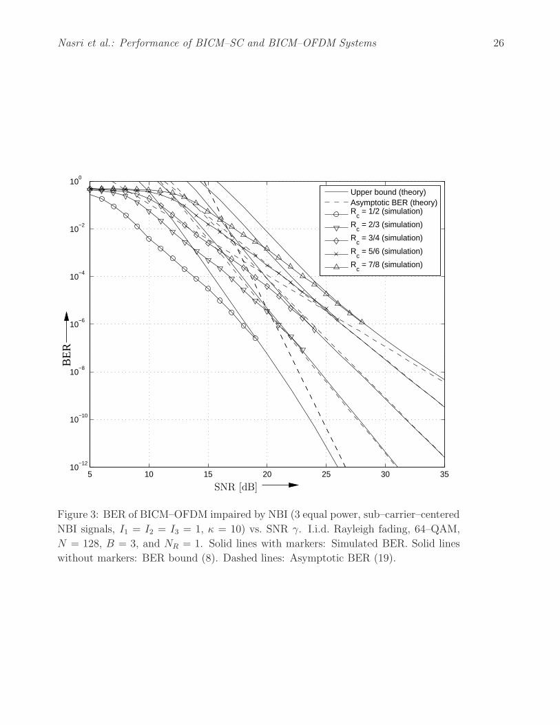
In Fig. 3, we investigate the effect of the code rate Rc on the performance of BICM–OFDM

(N = 128) in NBI for an i.i.d. Rayleigh fading channel and 64–QAM. Fig. 3 shows that as the code

rate decreases, the diversity gain increases since the free distance of the code increases, cf. (24). While

the approximate upper bound (solid line without markers) approaches the simulation results (solid lines

with markers) for BER < 10−6 in all cases, the convergence of the upper bound to the asymptotic

BER (dashed lines) is slower for small (Rc = 1/2) and large (Rc = 7/8) code rates. For Rc = 1/2, df

is large making the asymptotic BER curve very steep, which leads to an over–estimation of the BER at

low SNRs, cf. Section 4.2. For Rc = 7/8, the slow convergence can be explained by the large relative

weight of terms neglected in asymptotic BER expressions (e.g. w(df + 1)/w(df) = 56), cf. Section

4.2. For comparison, Rc = 3/4 shows a much faster convergence since w(df + 1)/w(df) = 5.

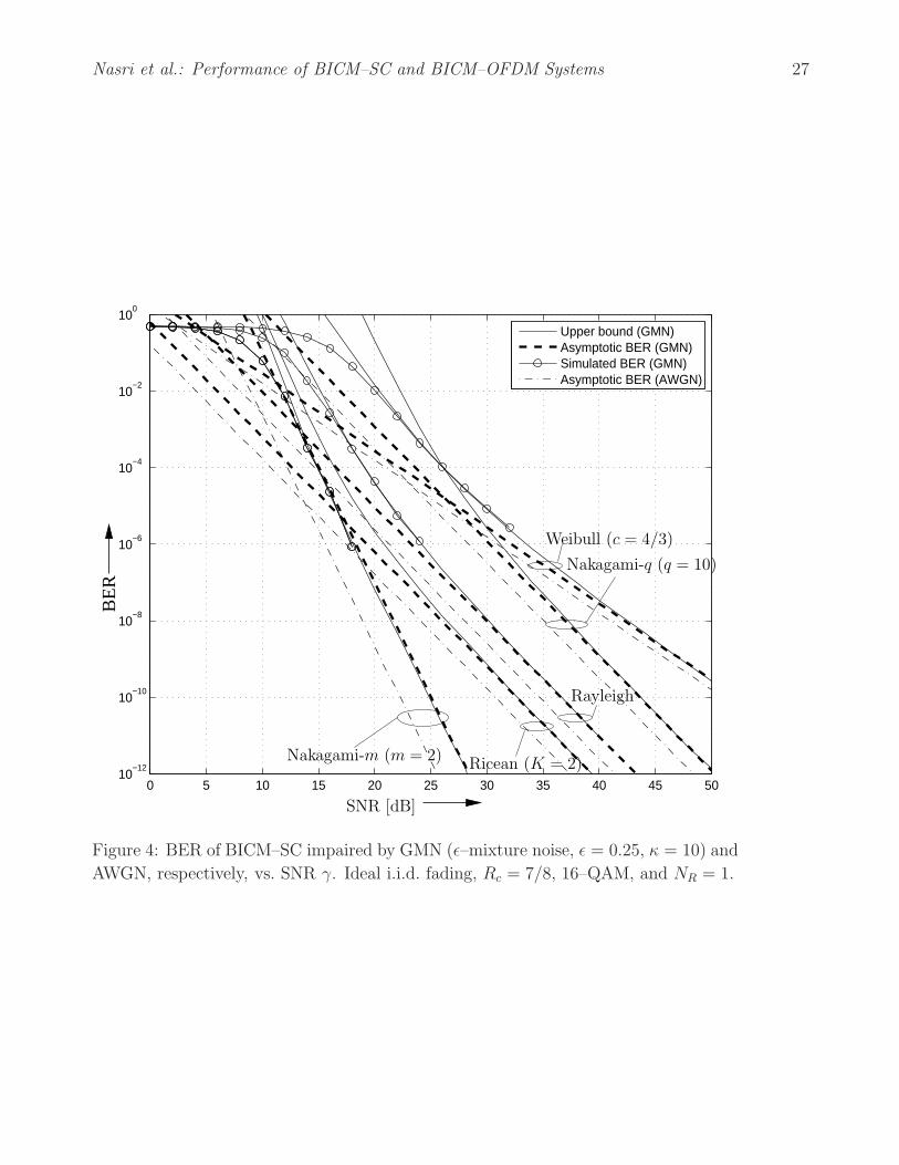
In Fig. 4, we consider the impact of the type of fading on the BER of BICM–SC with 16–QAM

for GMN and AWGN. Since the type of fading affects the diversity gain Gd = αddf , the asymptotic

slopes of the BER curves for Nakagami–m (αd = m = 2) and Weibull (αd = c/2 = 2/3) fading

differ from the asymptotic slopes of the BER curves for Rayleigh, Ricean, and Nakagami–q fading,

since for the latter three αd = 1 holds. It can also be observed that the performance loss caused by

GMN compared to AWGN decreases with decreasing diversity order.

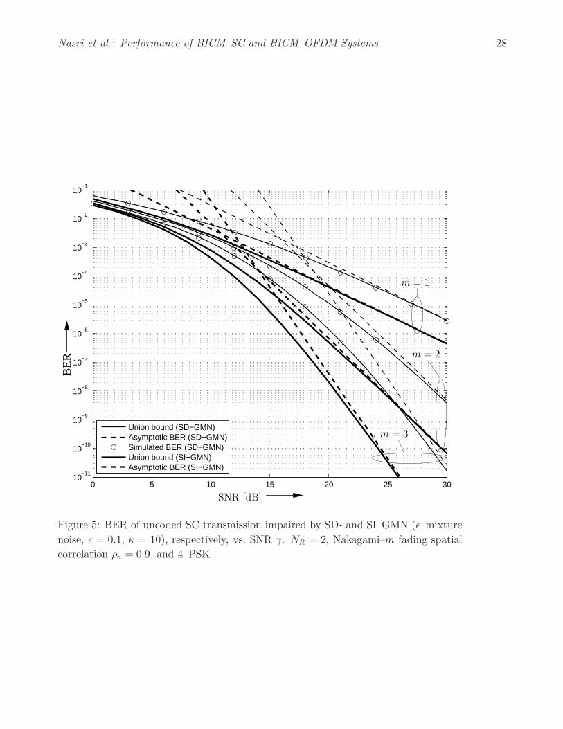
In Fig. 5, we show the BERs of uncoded SC transmission over correlated Nakagami–m channels

with NR = 2 receive antennas and impairment by SD- and SI–GMN (both cases: ǫ–mixture noise


with ǫ = 0.1, κ = 10). The spatial fading correlation coefficient is ρa = 0.9. Note that for uncoded

transmission the temporal i.i.d. asumption for fading and noise is not required. Fig. 5 shows that

for uncoded transmission the derived approximate upper bound is very tight even at low SNR and

approaches the asymptotic BER at high SNR. Thereby, the asymptotic BER converges faster to the

upper bound for channels with smaller diversity gain. Furthermore, Fig. 5 confirms that spatial noise

dependencies lead to significant performance degradations.

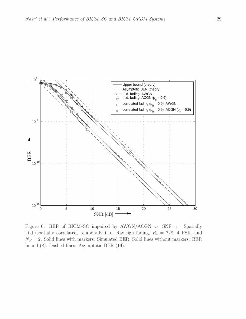
In Fig. 6, we consider the BER of BICM–SC impaired by temporally i.i.d., spatially uncorre-

lated/correlated (fading correlation ρh = 0.9) Rayleigh fading and AWGN/ACGN (noise correlation

ρn = 0.9) for NR = 2. Fig. 6 shows that, while noise correlation has also adverse effects on perfor-

mance, fading correlation is more harmful. Furthermore, the convergence of the asymptotic BER to

the approximate union bound is negatively affected by the spatial fading correlation.

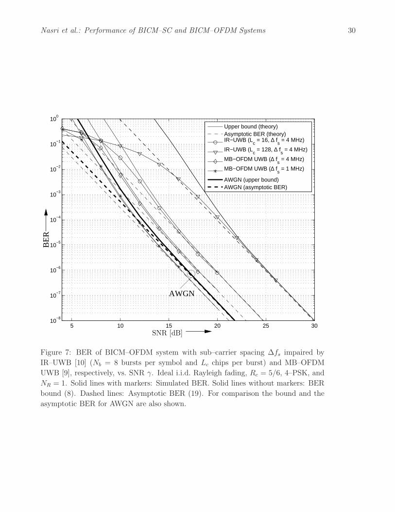
Finally, in Fig. 7, we consider the BER of BICM–OFDM impaired by UWB interference and

temporally i.i.d. Rayleigh fading. We consider MB–OFDM and impulse–radio UWB (IR–UWB) in-

terference following the EMCA [9] and the IEEE 802.15.4a [10] standards, respectively. Specifically,

for IR–UWB we assume Nb = 32 bursts per symbol and Lc chips per burst [10]. The MGF required

for the approximate upper bound (8) was obtained using the methods proposed in [11]. Since, due

to the complicated nature of the interference signal, closed–form expressions for the moments are

difficult to obtain, we used the Monte–Carlo approach discussed in Section 5.3 for calculation of the

moments for evaluation of the asymptotic BER (19). Fig. 7 nicely illustrates that the coding gain in

UWB interference strongly depends on the sub–carrier spacing of the victim BICM–OFDM system

and the format of the UWB interference. Interestingly, for ∆fs = 100 MHz MB–OFDM has a more

favorable noise pdf than AWGN and thus, is less detrimental to the performance of the BICM–OFDM

system than AWGN.

7 Conclusions

In this paper, we have presented a framework for performance analysis of BICM–SC and BICM–

OFDM systems impaired by fading and non–Gaussian noise and interference. The proposed analysis

is very general and applicable to all popular fading models (including Rayleigh, Ricean, Nakagami–

m, Nakagami–q, and Weibull fading) and all types of noise with finite moments (including AWGN,

ACGN, GMN, CCI, NBI, and UWB interference). In particular, we have derived an approximate upper


bound for the BER which allows for efficient numerical evaluation and a simple, accurate closed–form

approximation for the asymptotic BER. Our asymptotic analysis reveals that while the coding gain is

strongly noise dependent, the diversity gain of the overall system is not affected by the type of noise.

This result is important from a practical point of view since it shows that at high SNRs the BER

curves of BICM systems optimized for AWGN will only suffer from a parallel shift if the impairment

in a real–world environment is non–Gaussian.

A Spatially Correlated Fading Channels

In this appendix, we prove (2) for correlated Rayleigh, Ricean, and Nakagami–m fading.

Ricean Fading: For Ricean fading the pdf of the channel vector h is given by

ph(h) =1

πNR det(Chh)exp

[

−(h − µh)HC−1

hh (h − µh)]

, (40)

where µh , E{h} and Chh , E{(h − µh) (h−µh)H} are the channel mean and channel covariance

matrix, respectively. For h → 0NRwe can rewrite (40) as

ph(h) =exp

(

−µHh C−1

hhµh

)

πNR det(Chh)+ o(1). (41)

Based on (41) and the relation |hl|2 = a2l it can be shown that (2) and (3) hold for correlated

Rayleigh (µh = 0NR) and Ricean (µh 6= 0NR

) fading with αc and αd as specified in Table 1.

Nakagami–m Fading: For Nakagami–m fading the joint MGF of a2l , 1 ≤ l ≤ NR, is given by

[24]

Φa2(s) , E{

exp

(

−NR∑

l=1

a2l sl

)}

= det(INR+ SCaa/m)−m, (42)

where S , diag{s}, and Caa and m denote the channel correlation matrix and the fading parameter,

respectively. The behavior of the joint pdf pa2(a21, . . . , a2

NR) of a2

l , 1 ≤ l ≤ NR, for a → 0NRcan

be deduced from the behavior of Φa2(s) for sl → ∞, 1 ≤ l ≤ NR, which is given by

Φa2(s) = mNRm det(Caa)−m

NR∏

l=1

s−ml + o

(

NR∏

l=1

s−ml

)

. (43)

Consequently, we obtain

pa2(a21, . . . , a2

NR) = mNRm det(Caa)

−m

NR∏

l=1

a2(m−1)l

Γ(m)+ o

(

NR∏

l=1

a2(m−1)l

)

, (44)


which clearly shows that the al, 1 ≤ l ≤ NR, are asymptotically i.i.d., i.e., (2) and (3) are valid. The

corresponding parameters αc and αd are provided in Table 1 and can be obtained by exploiting the

relation between pa2(a21, . . . , a2

NR) and pa(a).

References

[1] G. Caire, G. Taricco, and E. Biglieri. Bit–Interleaved Coded Modulation. IEEE Trans. Inform.Theory, 44:927–946, May 1998.

[2] H. Bolcskei. MIMO–OFDM Wireless Systems: Basics, Perspectives, and Challenges. IEEEWireless Commun., 13:31–37, August 2006.

[3] A. Coulson. Bit Error Rate Performance of OFDM in Narrowband Interference with ExcissionFiltering. IEEE Trans. Wireless Commun., 5:2484–2492, September 2006.

[4] T.S. Rappaport. Wireless Communications. Prentice Hall, Upper Saddle River, NJ, 2002.

[5] A. Giorgetti and M. Chiani. Influence of Fading on the Gaussian Approximation for BPSK andQPSK with Asynchronous Cochannel Interference. IEEE Trans. Wireless Commun., 4:384–389,March 2005.

[6] S. Krusevac, P. Rapajic, and R. Kennedy. Channel Capacity Estimation for MIMO Systems withCorrelated Noise. In Proceedings of IEEE Global Telecom. Conf., pages 2812–2816, Dec. 2005.

[7] R. Prasad, A. Kegel, and A. de Vos. Performance of Microcellular Mobile Radio in a CochannelInterference, Natural, and Man-Made Noise Environment. IEEE Trans. Veh. Technol., 42:33–40,February 1993.

[8] D. Middleton. Statistical-physical Models of Man–made Radio Noise – Parts I and II.U.S. Dept. Commerce Office Telecommun., April 1974 and 1976.

[9] ECMA. Standard ECMA-368: High Rate Ultra Wideband PHY and MAC Standard. [Online]http://www.ecma-international.org/publications/standards/Ecma-368.htm, December 2005.

[10] IEEE P802.15.4a. Wireless Medium Access Control (MAC) and Physical Layer (PHY) Specifi-cations for Low-Rate Wireless Personal Area Networks (LR-WPANs). January 2007.

[11] A. Nasri, R. Schober, and L. Lampe. Performance Evaluation of BICM-OFDM Systems Impairedby UWB Interference. In Proceedings of IEEE Intern. Commun. Conf. (ICC), July 2008.

[12] V. Sethuraman and B. Hajek. Comments on ”Bit–Interleaved Coded Modulation”. IEEE Trans.Inform. Theory, 52:1795–1797, April 2006.

[13] P.-C. Yeh, S. Zummo, and W. Stark. Error Probability of Bit–Interleaved Coded Modulation inWireless Environments. IEEE Trans. Veh. Technol., 55:722–728, March 2006.

[14] E. Akay and E. Ayanoglu. Achieving Full Frequency and Space Diversity in Wireless Systems viaBICM, OFDM, STBC, and Viterbi Decoding. IEEE Trans. Commun., 54:2164–2172, December2006.

[15] A. Martinez, A. Guillen i Fabregas, and G. Caire. Error Probability Analysis of Bit–InterleavedCoded Modulation. IEEE Trans. Inform. Theory, 52:262–271, January 2006.

[16] A. Martinez, A. Guillen i Fabregas, and G. Caire. A Closed–Form Approximation for the ErrorProbability of BPSK Fading Channels. IEEE Trans. Wireless Commun., 6:2051–2054, June 2007.

[17] D. Rende and T. Wong. Bit–Interleaved Space–Frequency Coded Modulation for OFDM Sys-tems. IEEE Trans. Wireless Commun., 4:2256–2266, September 2005.


[18] Y. Li and J. Moon. Error Probability Bounds for Bit–Interleaved Space–Time Trellis CodingOver Block–Fading Channels. IEEE Trans. Inform. Theory, 53:4285–4292, November 2007.

[19] H. Nguyen and T. Bui. Bit–Interleaved Coded Modulation With Iterative Decoding in ImpulsiveNoise. IEEE Trans. Power Delivery, 22:151–160, January 2007.

[20] H. Abdel-Ghaffar and S. Pasupathy. Asymptotic Performance of M-ary and Binary Signals OverMultipath/Multichannel Rayleigh and Ricean Fading. IEEE Trans. Commun., 43:2721–2731,November 1995.

[21] Z. Wang and G. Giannakis. A Simple and General Parameterization Quantifying Performance inFading Channels. IEEE Trans. Commun., 51:1389–1398, August 2003.

[22] A. Nasri, R. Schober, and Y. Ma. Unified Asymptotic Analysis of Linearly Modulated Signals inFading, Non–Gaussian Noise, and Interference. IEEE Trans. Commun., 56:980–990, June 2008.

[23] A. Nezampour, A. Nasri, R. Schober, and Y. Ma. Asymptotic BEP and SEP of Quadratic Diver-sity Combining Receivers in Correlated Ricean Fading, Non–Gaussian Noise, and Interference.To appear in IEEE Trans. Commun. [Online] http://www.ece.ubc.ca/∼alinezam/TCOM-07.pdf,2008.

[24] M.K. Simon and M.-S. Alouini. Digital Communication over Fading Channels. Wiley, Hoboken,New Jersey, 2005.

[25] O.C. Ugweje and V.A. Aalo. Performance of Selection Diversity System in Correlated NakagamiFading. In Proceedings of IEEE Veh. Techn. Conf. (VTC), pages 1488–1492, May 1997.

[26] C. Tan and N. Beaulieu. Infinite Series Representations of the Bivariate Rayleigh and Nakagami-m Distributions. IEEE Trans. Commun., 45:1159–1161, October 1997.

[27] G.A. Tsihrintzis and C.L. Nikias. Performance of Optimum and Suboptimum Receivers in thePresence of Impulsive Noise Modeled as an Alpha-Stable Process. IEEE Trans. Commun.,43:904–914, Feb./Mar./Apr. 1995.

[28] E. Biglieri, G. Caire, G. Taricco, and J. Ventura-Traveset. Computing Error Probabilities overFading Channels: a Unified Approach. European Trans. Telecommun., 9:15–25, Jan./Feb. 1998.

[29] I. Gradshteyn and I. Ryzhik. Table of Integrals, Series, and Products. Academic Press, NewYork, 2000.

[30] C. Tepedelenlioglu and P. Gao. On Diversity Reception Over Fading Channels with ImpulsiveNoise. IEEE Trans. Veh. Technol., 54:2037–2047, November 2005.


Tables and Figures:

Table 1: Pdf pa(a) of fading amplitude a for popular fading models and corresponding valuesfor αc and αd. We have omitted subscript l for convenience. The parameters for Rayleigh(Chh), Ricean (µh, Chh), and Nakagami–m (m, Caa) fading are defined in Appendix A. Theparameters for Nakagami–q (q, b) and Weibull (c) fading are defined as in [24].

Channel type pa(a) of the fading amplitude a αc αd

Rayleigh 2 a e−a2

det(Chh)−1/NR 1

Ricean 2(K + 1) a e−K−(1+K)a2

I0

(

2a√

K(K + 1))

(

exp(

−µHh C−1

hhµh

)

det(Chh)

)1/NR

1

Nakagami–m 2Γ(m)

mm a2m−1 e−ma2 mm

Γ(m)det(Caa)

−m/NR m

Nakagami–q 2a√1−b2

exp(

− a2

(1−b2)

)

I0

(

ba2

(1−b2)

)

1+q2

2q1

Weibull c(

Γ(1 + 2c))

c2 ac−1 exp

(

−(

a2Γ(1 + 2c))

c2

)

c2(Γ(1 + 2

c))

c2

c2

Table 2: MGF Φn(s) and scalar moments Mn(i) of types of noise considered in Section 5. Allvariables in this table are defined in Section 5. (SC) and (OFDM) means that the type of noiseis relevant for BICM–SC and BICM–OFDM, respectively.

Noise type Noise MGF Φn(s) Scalar moment Mn(i)

AWGN (SC & OFDM) exp(s2/4) i!

GMN (SC)∑I

k=1 ck exp(s2σ2k/4) i!

∑Ik=1 ck σ2i

k

CCI (SC)∑B

µ=1

∑

Sµcµ,Sµ

exp(s2σ2Sµ

/4) i!∑B

µ=1

∑

Sµcµ,Sµ

σ2iSµ

GMN (OFDM)∑

k1+···+kI=N ck1,...,kIexp(s2σ2

k1,...,kI/4) i!

∑

k1+···+kI=N ck1,...,kIσ2i

k1,...,kI

NBI (OFDM)∑B

µ=1

∑Iµ

i=1

∑

k∈Nµ,ic0 exp(s2σ2

µ,i,k/4) i!(∑B

µ=1

∑Iµ

ν=1

∑

k∈Nµ,νc0σ

2iµ,ν,k

+c1 exp(s2σ2n/4) +c1σ

2in )


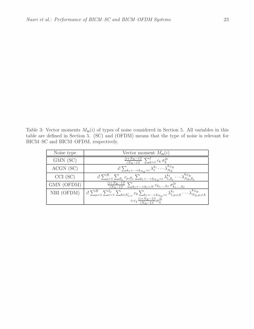
Table 3: Vector moments Mn(i) of types of noise considered in Section 5. All variables in thistable are defined in Section 5. (SC) and (OFDM) means that the type of noise is relevant forBICM–SC and BICM–OFDM, respectively.

Noise type Vector moment Mn(i)

GMN (SC) (i+NR−1)!(NR−1)!

∑Ik=1 ck σ2i

k

ACGN (SC) i!∑

k1+···+kNR=i λ

k1

1 · · ·λkNR

NR

CCI (SC) i!∑B

µ=1

∑

Sµcµ,Sµ

∑

k1+···+kNR=i λ

k1

1,Sµ· · ·λkNR

NR,Sµ

GMN (OFDM) (i+NR−1)!(NR−1)!

∑

k1+···+kI=N ck1,...,kIσ2i

k1,...,kI

NBI (OFDM) i!∑B

µ=1

∑Iµ

ν=1

∑

k∈Nµ,νc0

∑

k1+···+kNR=i λ

k1

1,µ,ν,k · · ·λkNR

NR,µ,ν,k

+c1(i+NR−1)!(NR−1)!

σ2in


0 5 10 15 20 2510

−9

10−8

10−7

10−6

10−5

10−4

10−3

10−2

10−1

100

Upper bound (theory)Asymptotic BER (theory)B = 3 (simulation)B = 5 (simulation)B = 10 (simulation)B = 15 (simulation)

BICM−SC

BE

R

BICM-OFDM (N = 128)

SNR [dB]

BICM-OFDM (N = 64)

Figure 1: BER of BICM–SC and BICM–OFDM impaired by GMN (ǫ–mixture noise,

ǫ = 0.1, κ = 100) and NBI, respectively, vs. SNR γ. Rc = 3/4, Rayleigh fading, 4–

PSK, and NR = 1. BICM–SC: Flat time–selective fading, N = 972, and BfT = 0.007.

BICM–OFDM (N = 64): Frequency–selective Rayleigh fading with L = 10 and B

equal power, sub–carrier centered NBI signals with Iµ = 1, 1 ≤ µ ≤ B, κ = 7. BICM–

OFDM (N = 128): Frequency–selective Rayleigh fading with L = 20 and B equal

power, sub–carrier centered NBI signals with Iµ = 1, 1 ≤ µ ≤ B, κ = 2. Solid lines

with markers: Simulated BER. Solid lines without markers: BER bound (8). Dashed

lines: Asymptotic BER (19).


0 5 10 15 20 25 3010

−10

10−9

10−8

10−7

10−6

10−5

10−4

10−3

10−2

10−1

100

Upper bound (theory)Asymptotic BER (theory)BICM−SC: GMN I (B = 10)BICM−SC: GMN II (B = 10)BICM−SC: Asynchronous CCI (B = 10)BICM−OFDM: GMN II (B = 15)BICM−OFDM: NBI (B = 5)AWGN (upper bound)AWGN (asymptotic BER)

BE

R

SNR [dB]

Figure 2: BER of BICM–SC and BICM–OFDM impaired by various types of noise

vs. SNR γ. Rayleigh fading, Rc = 3/4, 4–PSK, and NR = 1. BICM–SC: N = 972 and

BfT = 0.007. BICM–OFDM: N = 64 and L = 10. GMN I: ǫ–mixture noise, ǫ = 0.01,

κ = 100. GMN II: ǫ–mixture noise, ǫ = 0.1, κ = 100. Asynchronous CCI: Two

asynchronous equal power 4–PSK CCI signals, Iµ = 1, µ ∈ {1, 2}, Iµ = 0, 3 ≤ µ ≤ 10,

raised cosine pulses g1,µ(t), µ ∈ {1, 2}, with roll–off factor 0.3, τ1,µ = 0.3T , µ ∈ {1, 2},κ = 2. NBI: One sub–carrier–centered NBI signal, I1 = 1, I2 = I3 = I4 = I5 = 0,

κ = 9. Solid lines with markers: Simulated BER. Solid lines without markers: BER

bound (8). Dashed lines: Asymptotic BER (19).


5 10 15 20 25 30 3510

−12

10−10

10−8

10−6

10−4

10−2

100

Upper bound (theory)Asymptotic BER (theory)R

c = 1/2 (simulation)

Rc = 2/3 (simulation)




BE

R

SNR [dB]

Figure 3: BER of BICM–OFDM impaired by NBI (3 equal power, sub–carrier–centered

NBI signals, I1 = I2 = I3 = 1, κ = 10) vs. SNR γ. I.i.d. Rayleigh fading, 64–QAM,

N = 128, B = 3, and NR = 1. Solid lines with markers: Simulated BER. Solid lines

without markers: BER bound (8). Dashed lines: Asymptotic BER (19).


0 5 10 15 20 25 30 35 40 45 5010

−12

10−10

10−8

10−6

10−4

10−2

100

Upper bound (GMN)Asymptotic BER (GMN)Simulated BER (GMN)Asymptotic BER (AWGN)

BE

R

SNR [dB]

Nakagami-m (m = 2)

Rayleigh

Weibull (c = 4/3)

Nakagami-q (q = 10)

Ricean (K = 2)

Figure 4: BER of BICM–SC impaired by GMN (ǫ–mixture noise, ǫ = 0.25, κ = 10) and

AWGN, respectively, vs. SNR γ. Ideal i.i.d. fading, Rc = 7/8, 16–QAM, and NR = 1.


0 5 10 15 20 25 3010

−11

10−10

10−9

10−8

10−7

10−6

10−5

10−4

10−3

10−2

10−1

Union bound (SD−GMN)Asymptotic BER (SD−GMN)Simulated BER (SD−GMN)Union bound (SI−GMN)Asymptotic BER (SI−GMN)

BE

R

SNR [dB]

m = 2

m = 1

m = 3

Figure 5: BER of uncoded SC transmission impaired by SD- and SI–GMN (ǫ–mixture

noise, ǫ = 0.1, κ = 10), respectively, vs. SNR γ. NR = 2, Nakagami–m fading spatial

correlation ρa = 0.9, and 4–PSK.


0 5 10 15 20 25 3010

−15

10−10

10−5

100

Upper bound (theory)Asymptotic BER (theory)I.i.d. fading, AWGNI.i.d. fading, ACGN (ρ

n = 0.9)

correlated fading (ρh = 0.9), AWGN

correlated fading (ρh = 0.9), ACGN (ρ

n = 0.9)

BE

R

SNR [dB]

Figure 6: BER of BICM–SC impaired by AWGN/ACGN vs. SNR γ. Spatially

i.i.d./spatially correlated, temporally i.i.d. Rayleigh fading, Rc = 7/8, 4–PSK, and

NR = 2. Solid lines with markers: Simulated BER. Solid lines without markers: BER

bound (8). Dashed lines: Asymptotic BER (19).


5 10 15 20 25 3010

−8

10−7

10−6

10−5

10−4

10−3

10−2

10−1

100

Upper bound (theory)Asymptotic BER (theory)IR−UWB (L

c = 16, ∆ f

s = 4 MHz)

IR−UWB (Lc = 128, ∆ f

s = 4 MHz)

MB−OFDM UWB (∆ fs = 4 MHz)

MB−OFDM UWB (∆ fs = 1 MHz)

AWGN (upper bound)AWGN (asymptotic BER)

BE

R

AWGN

SNR [dB]

Figure 7: BER of BICM–OFDM system with sub–carrier spacing ∆fs impaired by

IR–UWB [10] (Nb = 8 bursts per symbol and Lc chips per burst) and MB–OFDM

UWB [9], respectively, vs. SNR γ. Ideal i.i.d. Rayleigh fading, Rc = 5/6, 4–PSK, and

NR = 1. Solid lines with markers: Simulated BER. Solid lines without markers: BER

bound (8). Dashed lines: Asymptotic BER (19). For comparison the bound and the

asymptotic BER for AWGN are also shown.

Documents

Performance of BICM–SC and BICM–OFDM Systems with ...amirn/TCOM-08.pdfNakagami–q, and Weibull fading) and general types of noise and interference with ﬁnite moments such as