Master Thesis in Finance

Spring 2012

Authors: Supervisor:

Amanda Kolobaric Jens Forssbaeck

Parisa Khatabakhsh

Performance of Hedge Funds in the

European Market

1

ABSTRACT

The aim of this paper is to investigate the performance of hedge funds during the period

between December 1999 and March 2012. We consider 8 different investment styles for the

European market. As it has been argued in several papers hedge funds differ from traditional

funds, since it allows for diversification and lower systematic risk. Previous studies show

inconclusive results regarding whether hedge funds are able to beat the market. In order to

find evidence for the existence of abnormal returns for the hedge funds we regress 3 different

asset pricing models, static CAPM, Fama-French three factor model and dynamic Multi-factor

model. In line with our expectations the Multi-factor model is better suited to capture the

dynamic risk exposures of the hedge funds since it includes additional risk factors as well as

instrumental variables, taking into account the effects of the business cycles. We investigate

the performance of the hedge funds in 3 different sub-periods and find that for some of the

investments strategies it is possible to obtain positive anomalies in returns. However, the

empirical results demonstrate that the number of significant alpha’s from the various models

change over time and strategies.

Keywords: Hedge funds, asset pricing models, Multi-factor model, investment strategies,

performance measures.

2

ACKNOWLEDGEMENTS

We would like to thank Professor Jens Forssbaeck for his guidance, responsiveness and on top

of all his valuable comments throughout this research process.

3

TABLE OF CONTENTS

1. INTRODUCTION .................................................................................................................. 5

1.1 Background .......................................................................................................................... 5

1.2 Problem Discussion .............................................................................................................. 6

1.3 Purpose ................................................................................................................................. 6

1.4 Limitations ............................................................................................................................ 6

1.5 Outline .................................................................................................................................. 6

2. THEORETICAL FRAMEWORK ......................................................................................... 7

2.1 Hedge Fund History ............................................................................................................. 7

2.2 Hedge Funds versus Traditional Investment Funds ............................................................. 7

2.3 Hedge Fund Definition ......................................................................................................... 8

2.4 Investment Strategies ............................................................................................................ 9

2.4.1 Directional Strategies ....................................................................................................... 9

2.4.2 Non-Directional Strategies ............................................................................................... 9

2.5 Previous Studies ................................................................................................................. 10

2.6 Asset Pricing Models .......................................................................................................... 12

2.6.1 CAPM .............................................................................................................................. 12

2.6.2 Fama-French Three Factor Model ................................................................................. 13

2.6.3 Conditional Factor Model ............................................................................................... 13

2.6.4 Risk Factors ..................................................................................................................... 14

2.6.5 Instruments ...................................................................................................................... 15

2.7 Performance Measures ...................................................................................................... 15

2.7.1 Jensen’s Alpha ................................................................................................................. 16

2.7.2 Sharpe Ratio .................................................................................................................... 16

2.8 Statistical Properties .......................................................................................................... 16

2.8.2 Autocorrelation ............................................................................................................... 17

2.8.2.1 Durbin-Watson statistics .............................................................................................. 17

2.8.3 Heteroskedasticity ........................................................................................................... 17

2.8.4 Multicollinearity .............................................................................................................. 18

2.8.5 Skewness .......................................................................................................................... 18

3. METHODOLOGY ............................................................................................................... 20

3.1 Motivation .......................................................................................................................... 20

3.2 General Method of Work .................................................................................................... 20

4

3.3 Data .................................................................................................................................... 21

3.4 Potential Biases .................................................................................................................. 22

4. EMPIRICAL RESULTS AND ANALYSIS ........................................................................ 24

4.1 Descriptive Statistics .......................................................................................................... 24

4.1.1 Multicollinearity .............................................................................................................. 26

4.2 CAPM ................................................................................................................................. 26

4.2.1 Results and Analysis ........................................................................................................ 27

4.3 Fama-French Three Factor Model .................................................................................... 29

4.3.1 Results and Analysis ........................................................................................................ 30

4.4 Conditional Factor Model .................................................................................................. 32

4.4.1 Result and Analysis ......................................................................................................... 33

5. CONCLUSION .................................................................................................................... 36

5.1 Further studies .................................................................................................................... 37

6. REFERENCES ..................................................................................................................... 38

7. APPENDIX .......................................................................................................................... 42

Table 7.1 Data statistics, first sub-period (December 1999 – December 2003) ........................................... 42

Table 7.2 Data statistics, second sub-period (January 2004 – December 2007) .......................................... 42

Table 7.3 Data statistics, third sub-period (January 2008 – March 2012) ................................................... 43

Table 7.4 Augmented Dickey-Fuller test for non-stationarity. ...................................................................... 43

Table 7.5 Results for Heteroskedasticity and autocorrelation for CAPM. .................................................... 44

Table 7.6 Results for Heteroskedasticity and autocorrelation, Fama-French Factor Model. ...................... 44

Table 7.7 Results for Heteroskedasticity and autocorrelation, Multi-Factor Model. ................................... 45

Table 7.8.Full conditional regression output for the entire period. .............................................................. 45

Table 7.9 Summarized Multi-Factor results for the entire period, December 1999 – December 2003. ....... 45

Table 7.10 Summarized Multi-Factor results for the entire period, January 2004 – December 2007. ........ 46

Table 7.11 Summarized Multi-Factor results for the entire period, January 2008 – March 2012. .............. 46

5

1. INTRODUCTION

In the introductory chapter we aim to provide the reader with the background of the topic, problem

discussion and specification on the current state of research which will constitute the foundation of the

purpose. In addition, limitations and comprehensive outline of the study will be presented.

1.1 Background

During the past two decades, we have seen 25 percent of growth in alternative investments

vehicles like hedge funds. With approximately 10 000 active hedge funds worldwide

estimated to be a $2 trillion industry (Hedge Fund Association), increasing their prominence

in the financial market and providing investors with opportunities to manage risks and achieve

absolute returns. Perhaps, mainly because of the beneficial features of hedge funds, unlike

mutual funds, containing low systematic risk due to its low correlation with traditional asset

classes as well as limited government oversight (Ackermann, C., McEnally, R., &

Ravenscraft, D., (1999), Liang, B. (1999), Agarwal, V., & Naik, N.Y. (2000)).

Despite the fact of recent focus on hedge funds, the alternative investment vehicle has been in

existence since the year of 1949 and can be attributed to Alfred W. Jones. As he created an

investment fund as a general investment partnership, he had the idea of a (non directional /

market neutral) hedge fund that involved taking a long position in undervalued assets and at

the same time taking short position in overvalued assets. This innovation enabled investors to

make large bets with limited resources by an effectively leveraged investment capital.

(Brown, S.J., Goetzmann, W.N., & Ibbotson, R.G., 1999)

In general, there have been evidence showing both positive (absolute) return and performance

persistence (Edwards, F.R., & Caglayan, M.O., 2001). Investing in mutual funds will on

average underperform passive investment strategies that typically don’t actively attempt to

profit from short term fluctuations. The basic idea of hedge funds is to reduce volatility and

risk, at the same time yield high absolute returns in both bull- and bear markets. Thus, by

employing different unconventional investment strategies will allow the hedge fund manager

to instantly adapt and benefit from the volatile market. (Agarwal, & Naik, (2000), Fung, W.,

& Hsieh, D.A., (2000), Edwards, F.R., & Caglayan, M.O., (2001)

6

1.2 Problem Discussion

With the intention of analyzing hedge fund performances the majority of previous studies

often use static/unconditional asset pricing models, such as CAPM and Fama-French three

factor model, ignoring the time variation and overall ignoring the changing state of economy.

The problem of these model have as a consequence shifted focus towards conditional models,

allowing for time variability in order to overcome problems associated with different

conditional models. However, as previous studies in the field have given numerous

inconclusive findings regarding hedge fund performance applying static models, we will

therefore consider a further throughout research in the field applying both unconditional and

conditional models. This is necessary from both academics as well as an investor’s point of

view, in order to both overcome these problems and finding whether hedge funds really do

add value in terms of return.

1.3 Purpose

The purpose of this paper is to investigate and contribute to our understanding of the

performance of European hedge funds given different hedge fund styles. With the intention of

finding whether it is possible to produce excess returns, we apply different performance

methods, both conditional and unconditional models.

1.4 Limitations

We conduct this investigation using data provided from Eurekahedge, based on a set of

currently active European hedge funds which covers the available data sample of returns

between December 1999 and March 2012, including two distress periods (IT-bubble and real

estate-bubble). We will consider the European region as one unit, as the European index

comprises funds that are allocated to Europe, rather than individual countries.

1.5 Outline

The following chapter will provide a presentation of relevant theoretical issues and empirical

findings. In chapter three, data selection and work procedure will be clarified and specified as

well as relevant asset pricing models in addition potential biases will be discussed. In the

fourth chapter we present and analyze empirical findings. The final chapter will contain the

most important conclusions and suggestions for further research in the field.

7

2. THEORETICAL FRAMEWORK

This chapter will explain the relevant theories. Firstly we will present historical background and

definition of hedge funds then followed by comparison to traditional investment vehicles. Additionally,

the reader will be given explanation of relevant past findings as well as asset pricing models,

performance measures and its risk factors and instruments. We conclude the chapter by reviewing

different statistical properties. The theoretical framework will stand as a good base for further

analysis of the empirical findings.

2.1 Hedge Fund History

The conception of a hedge fund goes back to the year of 1949, when Alfred W. Jones, an

Australian journalist, came to the idea of short selling the overvalued stocks and

simultaneously going long in undervalued ones. He found out that this investment style

known also as a market neutral strategy, would result in gaining profits no matter in which

direction the market moves. Thus, the returns would depend on investors’ skills in choosing

right stocks but not the overall market reactions. He used leverage to purchase more shares

and enhance the returns and at the same time stayed away from risk exposures by short

selling. This combination made his investment strategy conservative and reduced the effects

of the market movements. This market neutral strategy has been followed by most hedge

funds during 1970’s. Although the start was quit slowly, the numbers of the hedge funds rose

up quickly during 1990’s which also resulted in various investment strategies. (Brown,

Goetzmann, & Ibbotson, 1999)

2.2 Hedge Funds versus Traditional Investment Funds

According to empirical studies, there are several differences between hedge funds and mutual

funds. In contrast with traditional investment vehicles, due to their numerous investment

styles the systematic risk is lower for the hedge funds as they allow for diversification. Hedge

funds’ limited regulations facilitate the investment decision making for their managers,

meanwhile the special fee structure gives incentive to the managers to perform more in line

with investors’ interests compared to the mutual funds. In contrast with traditional funds, the

fee depends on the performance rather than size of the asset. Additionally, due to its higher

water mark, the fee is only achievable when the managers make up the previous losses which

can be counted as another motivation. Diverse return targets can also be considered as another

difference between these two types of funds. Hedge funds are absolute performers while on

the other hand mutual funds are relative performers as their performance judge against

benchmarks like S&P 500 index. All in all, most of the times hedge funds show better

performance than mutual funds. (Liang, 1999)

8

Another difference is the restricted availability of the hedge funds. Mutual funds are easily in

the access of all groups of people with different wealth level, whilst hedge funds are only on

hand for special group of investors with higher wealth. It is possible to make money out of

hedge funds even at the time of down market, since its performance is regardless of the

market’s movement. Fund managers’ personal investment in the hedge funds is more common

compared to the traditional funds. Besides, their measurement for performance differs, since

the successful mutual fund has to outperform the market index whereas the success of the

hedge fund relies on the higher return due to its risk exposures. (Anderlind, P., Eidolf, E.,

Holm, M., Sommerlau, P., 2003)

2.3 Hedge Fund Definition

The meaning of hedge funds commonly refers to a general limited investment partnership.

The word hedge stems from protecting your investments with the objective of mitigating risk

exposure and making absolute returns on their underlying investments from market

uncertainty, i.e. generating positive returns in both up and down markets (Brown, Goetzmann,

& Ibbotson, 1999). Hedge funds are of interest to both academics as well as investors due to

their return profiles that significantly differs from mutual funds (Fung & Hsieh, 2000).

However, with a minimum investment ranging from $250,000 to $10,000,000 or more, hedge

funds can undertake any financial instrument and non-traditional trading strategies

(directional- and non-directional) unlike other funds, hence allowing for diversification

opportunities. For this reason we have seen a steady growth of 25 percent in alternative

investment vehicles like hedge funds, meaning that both the number and capital controlled

have increased their prominence in the financial market. However, as a result of the rather

limited regulation, it is with difficulty to say how many active hedge funds really exist, as

there are no regulations of having publicly available information regarding the operations of

alternative investments like hedge funds. Currently, there approximately exist 10 000 reported

active hedge funds worldwide and the number is growing every day, estimated to be a $2

trillion industry (Hedge Fund Association). According to Anderlind et al. (2003) 80 percent of

the active hedge funds are located in US, 13 percent in UK, 4 percent in Asia and remaining 3

percent in Europe. Even if the European hedge fund market is still fairly small as well as new,

it is still regarded as the market with the highest current growth rate compared to others.

(Anderlind et al., 2003)

9

2.4 Investment Strategies

We will closer investigate 8 hedge fund strategies. In line with Agarwal and Naik (2000) we

separate the different strategies according to whether they are directional, non-directional or

miscellaneous.

2.4.1 Directional Strategies

Strategies with high correlation with the market utilize the market movements and are referred

as directional:

Long Short Equities: This investment style focuses on short selling the equities that are

overvalued and expected to decrease in value and buying long undervalued securities that are

likely to have increase in value. By this investment strategy the market risk can be neutralized

and it can produce optimal risk-adjusted returns. This style is a combination of three strategies

long equities, short equities and modest leverage.

Macro: This is a very elastic strategy since it is used in various markets that are expected to

give the best opportunities. This investment style is a combination of leverage and long

positions which has an effect on securities, currency rates, commodities, fixed incomes and

interest rates. Appropriate timing is the key element for success in this investment style.

CTA/Managed Futures: This strategy is known as Commodity Trading Advisors. This

strategy combines long and short positions in order to yield returns in both up- and down

markets. The funds generally invest in currency markets plus options and futures.

2.4.2 Non-Directional Strategies

In the case of low correlation with the market, the classic market neutral strategy is classified

as non-directional:

Event Driven: Investment strategy that focuses on investing in situations where there is some

form of corporate activity or change i.e. exploring inconsistencies in the markets before/after

corporate events takes place, by taking a position in undervalued security that is expected to

rise in value due to the event. These corporate activities can refer to merger and acquisitions

(M&A), recapitalizations or liquidations to mention few (Agarwal & Naik, 2000). The main

risk is tied to the probability of event not occurring.

10

Fixed Income: By employing fixed income strategy, the hedge fund manager is able to earn

relative value and maximize its arbitrage opportunities by exploiting price anomalies between

fixed income securities and derivatives. According to Agarwal and Naik (2000) the risk of the

fund varies and depend on duration, credit exposure and leverage employed.

Arbitrage: An investment approach that involves buying a security or other financial

instrument in one market and simultaneously shorting a similar instrument in another market.

Hence, hedge managers can profit from price anomalies as a result of market inefficiencies.

Relative Value: It is an investment strategy that consists of managers simultaneously taking

long and short positions in related financial instruments that are expected to appreciate and

depreciate respectively, by doing so it allows investors to profit from the relative value of the

instruments.

In addition to the main categories a third category will be presented, Multi-Strategy as it can

be applied across the sub-groups:

Multi-strategy: This strategy is a combination of several investment styles such as convertible

bond arbitrage, long short equity, statistical arbitrage and merger arbitrage. This

diversification allows for lower volatility as well as smoother returns. These positive returns

are not dependent on direction of the market movements.

2.5 Previous Studies

During the last decades there have been a lot of researches done concerning hedge funds as a

result of their fast growth and the performance of the hedge fund is controversial according to

different studies. Some investigators believe that hedge fund returns are worse than what have

been expected because of their several biases as well as their high fees (Malkiel & Saha

2005), while in contrast many of other studies show greater performance of hedge funds

compared with mutual funds.

Liang (1999) investigated the performance of hedge funds for a period of 5 years, starting

from January 1992 until December 1996. In line with Fung and Hsieh (1997), Liang (1999)

argue that an investor holding a hedge fund portfolio will gain more than the one holding a

traditional mutual fund portfolio, since the hedge fund allows for diversification among

11

different strategies which don’t have high correlation with each other. On the other hand, the

compensation of mutual fund is related to the fund size while the fee of the hedge fund

depends on its performance. According to his findings, hedge funds present higher Sharpe

ratios as well as lower betas which consequently results in a greater performance compared

with the traditional mutual funds.

Ackermann, McEnally and Ravenskraft (1999) studied the performance of the hedge funds

considering return, risk and managerial incentives from 1988 to 1995. They compared hedge

funds with both mutual funds and standard market indices and conclude that while hedge

funds do better than the former they still don’t outperform the latter. They explained the

superior performance of the hedge funds by referring to several characteristic such as their

elastic investment styles and enticement fees as well as less governmental regulation.

Brown, Goetzmann and Ibbotson (1999) analyzed the performance of the offshore hedge

funds in US as a representative of the industry since the offshore funds consist of the most

important hedge funds. By applying unconditional CAPM, they found the evidence for lower

average annual return as well as lower standard deviation of the offshore hedge funds

compared to S&P 500 index, for the same period as Ackermann, McEnally and Ravenskraft

(1999). Their empirical study resulted in finding positive risk-adjusted returns for offshore

funds measured by Jensen’s alpha and Sharpe ratios.

Edwards and Caglayan (2001) used monthly returns of eight different investment strategies

between January 1990 and August 1998. Their results signified the fact that the hedge funds

abnormal returns depend on the type of the investment styles. However, using conditional

multifactor models, only twenty five percent of the hedge funds of their sample provided

positive risk-adjusted excess returns measured by the significant estimated alphas. They also

found considerable performance persistence over one- and two year scopes. As they

mentioned in their article, managerial skills in addition to incentive payments of the hedge

funds could count as some reasonable explanations for their remarkable performance.

In line with Edwards and Caglayan (2001), Kat and Miffre (2003) applied multifactor models

in order to investigate the performance of the hedge funds during the period of 1990 to 2000.

However, in contrast with the results of Edwards and Caglayan (2001), more than three

quarter of the hedge funds in the sample yielded abnormal returns.

12

2.6 Asset Pricing Models

The factor models break down the return of the asset into different factors. These models

identify the risk factors and can be used to compute the sensitivities of the assets to these

factors. In general, factor models for asset returns are mostly used in order to decompose the

risk and return into reasonable components and estimate the anomalous returns of the assets.

They also measure the volatility of the returns as well as the covariance among them. These

models allow for predicting future returns in different situations.

2.6.1 CAPM

The one-factor Capital Asset Pricing Model, introduced by Sharpe, W. (1964) and Lintner, L.

(1965), implies that the security’s return can be explained adequately by the assets’ sensitivity

to the market portfolio (beta). This model also takes into account the market expected return

as well as the expected return of the risk free asset. Beta is the non-diversifiable risk which

calculates the riskiness of the asset compared to the market. The security will have more

volatility that the market if the beta is superior than one and vice versa. The higher the risk is

the higher the expected return will be.

CAPM is based on several basic assumptions. In this model the utility-maximizing investors

are risk averse and they only care about the variance and mean respectively as a measure of

risk and return. The information is the same among all the investors, implying homogenous

expectations. In other words, by using the same inputs, investors expect the same amount of

risk and return. Besides, asset prices take into account all the accessible public information

and rapidly adjust to the new information released in the market. The market is also assumed

to be complete i.e. there are no taxes and transaction costs, the prices are not affected by

investors and at the risk free rate limitless borrowing and lending is permitted. The portfolio

lies on the efficient frontier so it can be optimized by having the lowest possible level of risk

for its level of return. In order to analyze the performance of the hedge funds we consider the

excess returns yielded by the eight different strategies in Europe. Sharpe and Lintner (1964)

hence argue that if investors hold homogenous expectations, mean-variance efficient portfolio

and the markets are assumed to be complete, the portfolio will itself will be considered to be a

mean-variance efficient portfolio. We apply CAPM by running the OLS time series

regression:

13

Whereas Rit is the expected monthly return of each hedge fund’s investment style at time t, Rft

is the risk free rate (one month Treasury bill rate), Rmt is the return on the market portfolio, εt

represents the error term. α and β are regression parameters. We run the regression in terms of

excess returns (Rit – Rft) on the market risk premium, (Rmt – Rft). The beta coefficient stands

for the measure of risk. (Campbell, J.Y., Lo, A.W., & Mackinlay, A.C., 1997)

2.6.2 Fama-French Three Factor Model

In order to describe the stock returns, in contrast with one variable CAPM, Fama, E. and

French K.R. (1992) introduced the three factor model which was superior in explicating asset

returns over time. They discuss the fact that average returns are also related to other risk

factors such as size and book-to-market value, since the traditional asset pricing model’s risk

factor solely wouldn’t be able to capture these return anomalies. So as to investigate the

performance of hedge funds we use Fama-French three factor model:

β, γ and δ are counted as the factor sensitivities of returns. (Rm – Rf) is the market risk

premium. SMB, is the measure for the size premium and HML accounts for value- over

growth stocks (Fama & French, (1996), Ogden, J.P., Jen, F.C. & O’Connor, P.F, (2002)).

2.6.3 Conditional Factor Model

Ferson and Schadt (1996) state that in the case of having time varying mean and variance, the

unconditional CAPM and Fama-French three factor model are not reliable since they can’t

capture the dynamics. They investigated the performance of fund strategies in changing

economic conditions.

Conditional factor approach was proposed by Ferson and Harvey (1999) in order to allow for

time-varying parameters as linear functions of instruments. Such instruments or conditioning

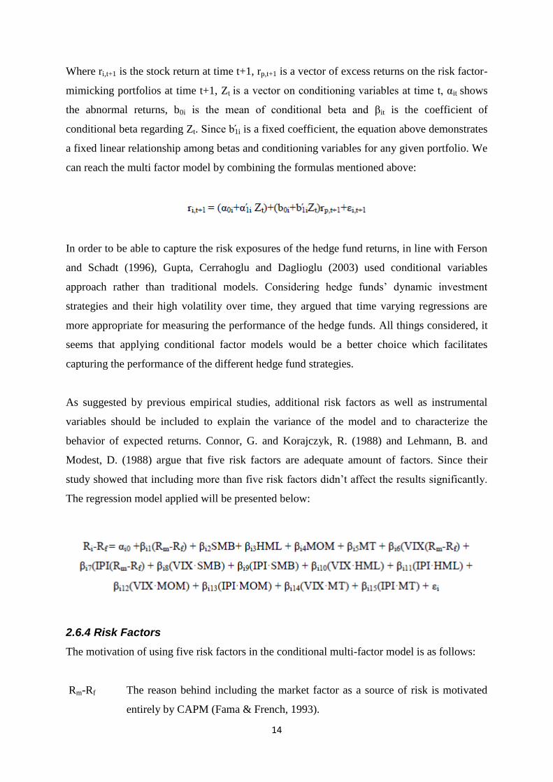
variables could represent the different economic conditions such as business cycles. Ferson

and Harvey (1999) introduced the general framework for conditional factor models:

14

Where ri,t+1 is the stock return at time t+1, rp,t+1 is a vector of excess returns on the risk factor-

mimicking portfolios at time t+1, Zt is a vector on conditioning variables at time t, αit shows

the abnormal returns, b0i is the mean of conditional beta and βit is the coefficient of

conditional beta regarding Zt. Since b 1i is a fixed coefficient, the equation above demonstrates

a fixed linear relationship among betas and conditioning variables for any given portfolio. We

can reach the multi factor model by combining the formulas mentioned above:

In order to be able to capture the risk exposures of the hedge fund returns, in line with Ferson

and Schadt (1996), Gupta, Cerrahoglu and Daglioglu (2003) used conditional variables

approach rather than traditional models. Considering hedge funds’ dynamic investment

strategies and their high volatility over time, they argued that time varying regressions are

more appropriate for measuring the performance of the hedge funds. All things considered, it

seems that applying conditional factor models would be a better choice which facilitates

capturing the performance of the different hedge fund strategies.

As suggested by previous empirical studies, additional risk factors as well as instrumental

variables should be included to explain the variance of the model and to characterize the

behavior of expected returns. Connor, G. and Korajczyk, R. (1988) and Lehmann, B. and

Modest, D. (1988) argue that five risk factors are adequate amount of factors. Since their

study showed that including more than five risk factors didn’t affect the results significantly.

The regression model applied will be presented below:

2.6.4 Risk Factors

The motivation of using five risk factors in the conditional multi-factor model is as follows:

Rm-Rf The reason behind including the market factor as a source of risk is motivated

entirely by CAPM (Fama & French, 1993).

15

SMB: Liew, J. and Vassalou, M. (2000) argue that SMB captures innovations in

economic growth expectations and inflation. According to Fama and French

(1993) small caps are riskier than large caps and therefore will yield higher

absolute returns and are hence a proxy for the size risk.

HML: According to Fama and French (1993) the book-to-market ratio is related to

higher return and in line with Liew and Vassalou (2000) HML would capture

information that is relevant in predicting the economic growth.

MOM: The explanation of including MOM as a risk factor is utterly based on results

and recommendations from Carhart’s (1997), Liew and Vassalou’s (2000) and

Jegadeesh, N. and Titman, S. (1993).

MT: Previous studies have showed inconclusive findings regarding the managers

market timing ability (Chen, L., & Liang, B., (2007), Fung, H.G, Xu, W.E., &

Yau, J., (2002)).

2.6.5 Instruments

The instrumental variables included, is used as proxies for the overall market condition and

business cycles, as a way of capturing the time variability.

VIX: Similar to Whaley, R.E. (2000) we ought to include the volatility index.

IPI: As the European gross domestic product is reported quarterly, construction of

monthly values would create certain biases, we therefore choose to include

industrial productivity as a proxy for business cycles in Europe.

2.7 Performance Measures

With the purpose of estimating the performance of the hedge funds in Europe from December

1999 to March 2012, we use two distinguished performance measures, Jensen’s alpha and the

Sharpe ratio.

16

2.7.1 Jensen’s Alpha

Jensen’s alpha is the intercept of asset pricing models which shows the performance of the

returns. CAPM returns are risk-adjusted as they allow for all the riskiness of the assets. The

positive Jensen’s index is a sign for the existence of positive abnormal returns in other words

it indicates higher asset returns compared to risk-adjusted returns. If the alpha is equal to zero

we will have the standard CAPM.

2.7.2 Sharpe Ratio

The Sharpe index is a measure of risk premium per each unit of risk which shows the balance

between the taken risk and expected return on the asset. Comparing two assets, the one with

higher Sharpe ratio indicates higher return for the same level of risk.

This index is calculable from any series of returns even with the lack of extra information

about the sources of profitability. However, despite this advantage, for reliable results the data

should be normally distributed so anomalies such as skewness or kurtosis may cause some

problems for this ratio.

2.8 Statistical Properties

To enable reliable empirical conclusions we need to consider some statistical properties. In

regression analysis, when applying time series data one needs to find whether the data can be

considered as being valid. Generally, when applying OLS with the purpose of estimating

parameters it is essential to find the data to be BLUE (Best Linear Unbiased Estimator),

showing the lowest possible mean squared error (MSE). If tests signify autocorrelation and/or

heteroskedasticity within the regression, as a consequence the results will no longer be

considered BLUE. Hence adjustments of data will be needed in order to obtain efficient and

reliable estimators, otherwise confidence intervals and hypothesis tests will be ambiguous.

Further on, we will examine various statistical properties.

17

2.8.1 Stationarity

According to Brooks (2008) we ought to test the data for non-stationarity, in order to find out

whether we can reject the null of unit root, against the alternative hypothesis of stationarity.

We perform an Augumented Dickey-Fuller (ADF) test type and use the test-statistic,

following DF-critical values in additional to the probability, in order to find whether we can

reject the null or not.

2.8.2 Autocorrelation

Autocorrelation is related to the problem of residuals being serially dependent of each other.

As the presence of positive serial correlation violates the OLS assumption, we will have to

account for problems related to statistical tests not being valid and reliable due to misleading

standard errors. To facilitate the problem, we initially need to examine the presence of

autocorrelation which can be done by applying traditional tests like Durbin-Watson statistics.

2.8.2.1 Durbin-Watson statistics

In line with Durbin J. and Watson G.S. (1951) we test the null that the errors are serially

independent against the presence of first order autocorrelation. The test statistics is

et is the residual at time t. If d>1, this implies positive serial correlation, whilst d<3 shows

evidence of negative autocorrelation. The rule of thumb signifies that d=1 indicates no

autocorrelation.

2.8.3 Heteroskedasticity

When the variance of the errors are not constant and finite, var(et) ≠ σ2

this will be of concern

in the application of regression analysis, as the presence will make the statistical tests invalid

(Brooks, C., 2008). The case with heteroskedasticity will as a fact not imply biased OLS

estimators, but will involve biased residuals. Consequently, the data will provide deceiving

standard errors and our inferences might as a result not be correct. We use the statistical test

called the White test in order to establish whether the residual variance is constant, var(et)=σ2.

Thus, we test the null of no heteroskedasticity against the presence of heteroskedasticity

18

(White, H., 1980). If the auxiliary regression analysis demonstrates that the dataset contains

heteroskedastic residuals one needs to apply the heteroskedastic-consistent covariance matrix

estimator in order to ensure unbiased residuals by adjusting the p-values.

2.8.4 Multicollinearity

When there is a relationship between two or more independent variables in a multiple

regression one might say that the regression suffers from multicollinearity. An important

statistical issue that is tied to the problem with collinearity and needs to be considered, is

related to spurious regressions. In order to identify this problem we will apply a correlation

matrix between all the explanatory variables, according to Brooks (2008) a correlation

coefficient in the range of 80% has to be considered. As a possible remedy Brooks (2008)

suggests one to exclude the variable that hold the highest level of correlation.

2.8.5 Skewness

The skewness is referred to the third standardized moment of a random variable and defined

as:

In order to detect the distribution of the hedge fund returns, one needs to take into

consideration the skewness. It is a measure of the asymmetry of the probability distribution of

stochastic variable. For left-skewed or left-tailed distribution, the skewness is negative and

vice versa. (Gujarati, D., 2006)

2.8.6 Kurtosis

Similar to skewness, kurtosis is another measure which describes the shape of the probability

distribution. However, unlike with skewness, this measure is based on the fourth moment of

the return data. Kurtosis can clarify the fatness of the distribution’s tails. The fourth

standardized moment minus 3 is defined as excess kurtosis which is used as an adjusted

version of kurtosis.

19

The formula indicates that for a normal distribution, the excess kurtosis should be zero so the

kurtosis would be three. Positive excess kurtosis means that the distribution has fatter tails and

higher peaks around the mean. This is also known as leptokurtic distribution while on the

other hand a platykurtic distribution with negative excess kurtosis contains thinner and lower

peaks around the mean. (Gujarati, 2006)

2.8.7 Normality

In order to check whether the returns have normal distribution, the Jarque-Bera test is

applicable. This test checks if the skewness and kurtosis of the data is close to a normal

distribution. The null hypothesis tests out whether skewness and excess kurtosis are jointly

equal to zero in other words if the sample returns are normally distributed. For the normally

distributed data, JB has a chi-squared distribution with two degrees of freedom.

20

3. METHODOLOGY

The following chapter will clarify and motivate the data selection process and the general method of

work in addition to specifying the chosen risk factors, pre-determined conditioning variables and

conclude the chapter with potential biases.

3.1 Motivation

As the objective for this research is to evaluate the performance of different hedge fund

strategies throughout different market conditions, we are therefore aiming to investigate

whether hedge fund managers are capable of producing excess returns. Furthermore, we use

quantitative data and empirically testing eminent performance models following a deductive

approach, i.e. by starting with hypothesis and then collect empirical data in order to find

whether we can reject or not reject our hypothesis and thereon draw conclusions. In line with

Jacobsen D.I. (2002) and Halvorsen K. (1992) we believe that the deductive approach is the

best suited and seem logical for the purpose of the investigation as well as to capture the

concepts of reality.

3.2 General Method of Work

To begin with, we collect our data sample from diverse databases during the period between

December 1999 and March 2012 consisting of 148 monthly observations for 8 different hedge

fund investment styles, with the motivation of being able to capture the excess returns in both

down- and up markets as we include both IT bubble as well as real-estate bubble. We

transformed the price index into returns with the following formula:

We obtained the monthly excess returns by taking the difference between Ri and the one

month T-bill, Rf. The excess returns are then estimated using Ordinary Least Squared (OLS)

against various independent variables. The estimations are performed on CAPM, Fama-

French Three factor model and a Conditional Multi-factor model which allows for time-

variability. Additionally, we test whether the data suffers from autocorrelation and

heteroskedasticity. In order to improve the OLS regression, we apply the Newey-West

estimator to adjust for autocorrelation and heteroskedasticity (HAC).

21

3.3 Data

The theoretical population corresponds to all the European countries, as indices are more

precise we believe that using the equally weighted index tracking the Europe industry would

be sufficient to capture the reality. The data sample is brought from different sources

including the Eurekahedge database where we found 148 monthly returns (net of all fees)

observations for 8 hedge fund styles since December 1999, to ensure a sufficient number of

consecutive observations to test some of the theories discussed. Other sources include

Thomson Reuters DataStream and Kenneth R. French data library.

Since neither daily nor weekly return data were available, the motivation of using monthly-

instead of annual returns, apart from giving more observations, enables us to track the hedge

fund return fluctuations more closely as well as enhances the accuracy of the standard

deviations. (Ackermann, McEnally, & Ravenscraft (1999), Brown, Goetzmann, & Ibbotson

(1999))

Further, we will present the sources of our risk factors and pre-determined conditioning

variables:

Ri: The return on 8 European hedge fund investment styles, including Arbitrage,

CTA/Managed Futures, Event Driven, Fixed Income, Long Short Equities,

Macro, Multi-Strategy, Relative Value and the data sample is obtained from

Eurekahedge.

RM: Is the market return on the whole stock market and used as a proxy for the

market (Fama & French, 2003). The data is obtained from Kenneth R. French

data library.

Rf: Stands for the risk free return rate (one month T-bill), collected from the

Kenneth R. French data library.

Rm-Rf Is consequently the excess return on the market.

SMB: Represents the spread in the returns between low-book-to-market stocks and

high-book-to-market stocks and constructed by forming value weighted

22

portfolios on size and BM (book-to-market) and measures the past excess

returns of small- over big caps. Data is obtained from the Kenneth R. French

data library.

HML: The data is obtained from Kenneth R. French data library and represents the

spread in the returns between high B/M and low B/M stocks. HML accounts for

the past excess returns of value- over growth stocks.

MOM: Momentum represents the difference between the average return on the portfolio

of past winners and portfolio of past loser.

MT: Is the market timing factor, max[(Rm-Rf)2, 0], the risk factor investigates if the

fund manager can account for the market timing ability, managers exhibiting

market timing ability will be able to earn higher abnormal returns when markets

are expected to rise and vice versa (Gupta et. al., 2003).

The pre-determined conditioning variables are:

VIX: The volatility index VSTOXX stands as a measure of the market’s perception of

risk and are designed to reflect market expectations of volatility in the European

equity market. The VIX-data is obtained from DataStream.

IPI: Industrial productivity measures the real production output and is used as a

proxy for business cycles in Europe. The data for industrial productivity is

monthly and given by DataStream. As the data for IPI exhibit seasonal

variation, for each month we use the average of the previous 12-months to

adjust and remove this cyclic variation.

3.4 Potential Biases

Whilst interpreting empirical results one needs to have potential biases in mind, as with

almost any base of data source there is a risk of hedge fund returns containing a variety of

biases that could affect the empirical findings.

23

Hedge fund research has confirmed the existence of a positive relationship between volatility

and fund disappearance (Ackermann, McEnally, & Ravenscraft, 1999). In general, when it

comes to survivorship biases we usually distinguish between surviving funds and defunct

funds. Whereas the surviving funds are still operating (alive) and present in the database as

opposed to defunct funds that have left the database (Fung, W., & Hsieh, D.A., (2000),

Malkiel, B., & Saha, A., (2005)). We are applying data from Eurekahedge, equal weighted

index for Europe. In order to eliminate the effects of survivorship they track down the

historical returns of funds that died and keep in the sample for the period they were alive as

well as including funds that are closed for further capital inflows.

Fung and Hsieh (2000) claim that selection biases might occur when return data are not

representative of the overall population, due to lack of regulations within the hedge fund

industry. Edwards and Caglayan (2001) argue that the selection bias that is caused by the

voluntary reporting might very well result in over- and underestimation of the hedge fund

performance, possibly affecting the returns both positively and negatively. In contrast Fung

and Hsieh (2000) argue that if the bias exists at all, it’s probably very small.

Another potential bias, the so called multi period sampling bias refers to return history.

Conducting empirical tests, it is of great importance to have reliable data in order to enable

future predictions. To enable more accurate and reliable results from empirical testing, one

needs sufficient return data. According to Ackermann, McEnally and Ravenscraft (1999) and

in line with Edwards and Caglayan (2001) a minimum of 24 months of return history is

required, although, Fung and Hsieh (2000) argue that the effect of the usage of shorter return

histories is relatively small. Therefore we believe that 148 months (per hedge fund style)

return data is sufficient in order overcome potential bias related to sample history.

24

4. EMPIRICAL RESULTS AND ANALYSIS

In the chapter we will present our empirical findings and analyze the results from the different asset

pricing models. To begin with, we will discuss some descriptive statistics, followed by analysis of

results which will be separated according to the different asset pricing models.

4.1 Descriptive Statistics

Before we start to investigate the performance of the hedge funds it is relevant to check for

the explanatory statistics of the hedge fund returns data for all the 8 different investment

strategies during the whole period.

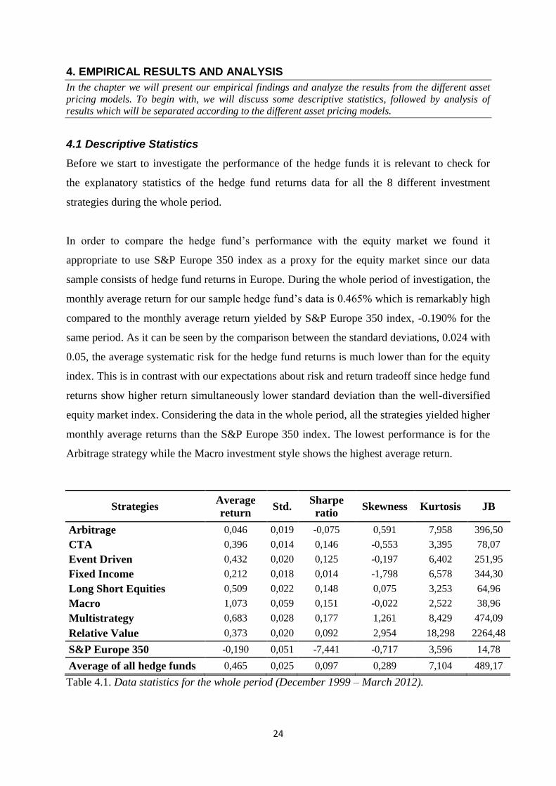
In order to compare the hedge fund’s performance with the equity market we found it

appropriate to use S&P Europe 350 index as a proxy for the equity market since our data

sample consists of hedge fund returns in Europe. During the whole period of investigation, the

monthly average return for our sample hedge fund’s data is 0.465% which is remarkably high

compared to the monthly average return yielded by S&P Europe 350 index, -0.190% for the

same period. As it can be seen by the comparison between the standard deviations, 0.024 with

0.05, the average systematic risk for the hedge fund returns is much lower than for the equity

index. This is in contrast with our expectations about risk and return tradeoff since hedge fund

returns show higher return simultaneously lower standard deviation than the well-diversified

equity market index. Considering the data in the whole period, all the strategies yielded higher

monthly average returns than the S&P Europe 350 index. The lowest performance is for the

Arbitrage strategy while the Macro investment style shows the highest average return.

Strategies Average

return Std.

Sharpe

ratio Skewness Kurtosis JB

Arbitrage 0,046 0,019 -0,075 0,591 7,958 396,50

CTA 0,396 0,014 0,146 -0,553 3,395 78,07

Event Driven 0,432 0,020 0,125 -0,197 6,402 251,95

Fixed Income 0,212 0,018 0,014 -1,798 6,578 344,30

Long Short Equities 0,509 0,022 0,148 0,075 3,253 64,96

Macro 1,073 0,059 0,151 -0,022 2,522 38,96

Multistrategy 0,683 0,028 0,177 1,261 8,429 474,09

Relative Value 0,373 0,020 0,092 2,954 18,298 2264,48

S&P Europe 350 -0,190 0,051 -7,441 -0,717 3,596 14,78

Average of all hedge funds 0,465 0,025 0,097 0,289 7,104 489,17

Table 4.1. Data statistics for the whole period (December 1999 – March 2012).

25

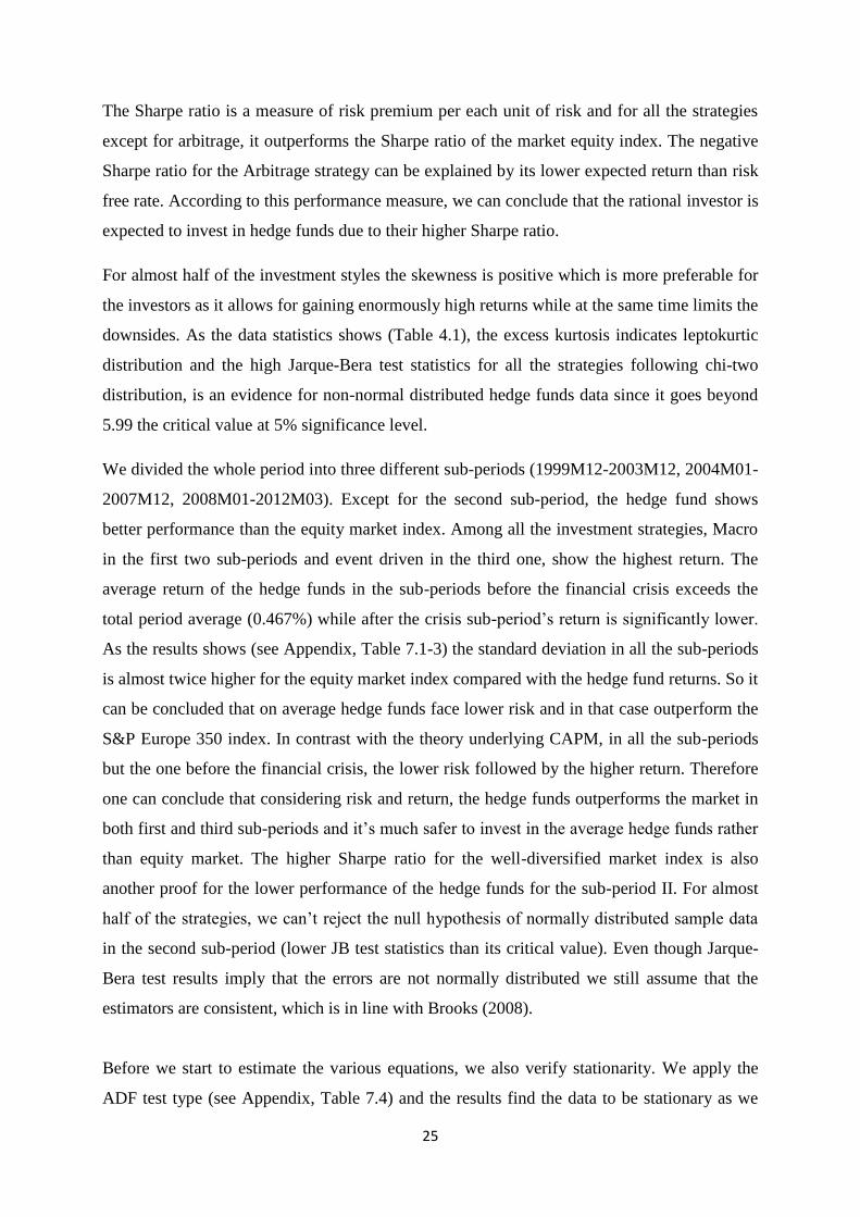
The Sharpe ratio is a measure of risk premium per each unit of risk and for all the strategies

except for arbitrage, it outperforms the Sharpe ratio of the market equity index. The negative

Sharpe ratio for the Arbitrage strategy can be explained by its lower expected return than risk

free rate. According to this performance measure, we can conclude that the rational investor is

expected to invest in hedge funds due to their higher Sharpe ratio.

For almost half of the investment styles the skewness is positive which is more preferable for

the investors as it allows for gaining enormously high returns while at the same time limits the

downsides. As the data statistics shows (Table 4.1), the excess kurtosis indicates leptokurtic

distribution and the high Jarque-Bera test statistics for all the strategies following chi-two

distribution, is an evidence for non-normal distributed hedge funds data since it goes beyond

5.99 the critical value at 5% significance level.

We divided the whole period into three different sub-periods (1999M12-2003M12, 2004M01-

2007M12, 2008M01-2012M03). Except for the second sub-period, the hedge fund shows

better performance than the equity market index. Among all the investment strategies, Macro

in the first two sub-periods and event driven in the third one, show the highest return. The

average return of the hedge funds in the sub-periods before the financial crisis exceeds the

total period average (0.467%) while after the crisis sub-period’s return is significantly lower.

As the results shows (see Appendix, Table 7.1-3) the standard deviation in all the sub-periods

is almost twice higher for the equity market index compared with the hedge fund returns. So it

can be concluded that on average hedge funds face lower risk and in that case outperform the

S&P Europe 350 index. In contrast with the theory underlying CAPM, in all the sub-periods

but the one before the financial crisis, the lower risk followed by the higher return. Therefore

one can conclude that considering risk and return, the hedge funds outperforms the market in

both first and third sub-periods and it’s much safer to invest in the average hedge funds rather

than equity market. The higher Sharpe ratio for the well-diversified market index is also

another proof for the lower performance of the hedge funds for the sub-period II. For almost

half of the strategies, we can’t reject the null hypothesis of normally distributed sample data

in the second sub-period (lower JB test statistics than its critical value). Even though Jarque-

Bera test results imply that the errors are not normally distributed we still assume that the

estimators are consistent, which is in line with Brooks (2008).

Before we start to estimate the various equations, we also verify stationarity. We apply the

ADF test type (see Appendix, Table 7.4) and the results find the data to be stationary as we

26

are able to reject the null. As we include intercept in our estimations we can be sure that

E(ut)=0 holds. Test results of the remaining OLS assumptions will be discussed below, in the

end we believe that our parameters are BLUE, as the results and adjustments ensure the

validity of inferences made.

4.1.1 Multicollinearity

RM_RF SMB HML MOM MT VIX IPI

RM_RF 1

SMB 0,312 1

HML -0,140 -0,384 1

MOM -0,349 0,145 -0,124 1

MT 0,726 0,246 -0,128 -0,370 1

VIX 0,020 0,032 -0,235 -0,184 0,268 1

IPI -0,165 -0,112 -0,121 0,017 -0,191 -0,138 1

Table 4.2. Correlation between independent variables.

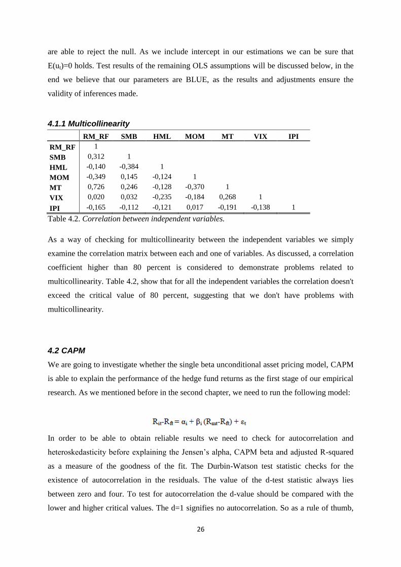
As a way of checking for multicollinearity between the independent variables we simply

examine the correlation matrix between each and one of variables. As discussed, a correlation

coefficient higher than 80 percent is considered to demonstrate problems related to

multicollinearity. Table 4.2, show that for all the independent variables the correlation doesn't

exceed the critical value of 80 percent, suggesting that we don't have problems with

multicollinearity.

4.2 CAPM

We are going to investigate whether the single beta unconditional asset pricing model, CAPM

is able to explain the performance of the hedge fund returns as the first stage of our empirical

research. As we mentioned before in the second chapter, we need to run the following model:

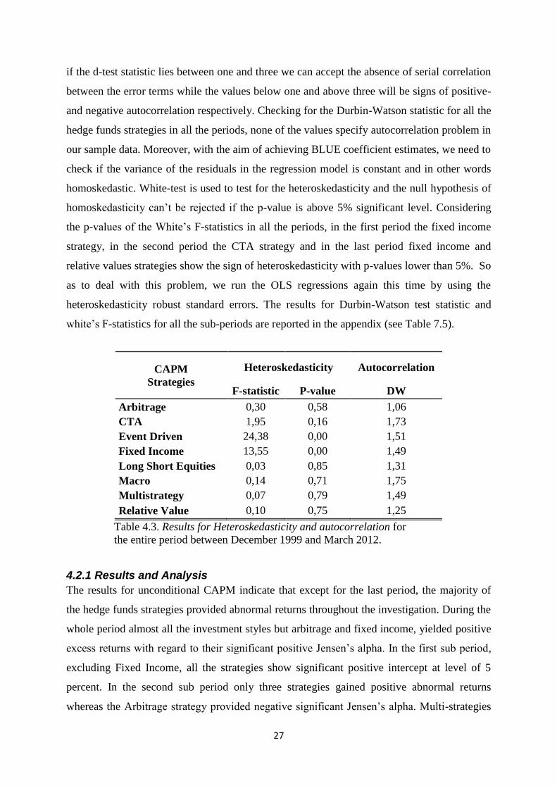
In order to be able to obtain reliable results we need to check for autocorrelation and

heteroskedasticity before explaining the Jensen’s alpha, CAPM beta and adjusted R-squared

as a measure of the goodness of the fit. The Durbin-Watson test statistic checks for the

existence of autocorrelation in the residuals. The value of the d-test statistic always lies

between zero and four. To test for autocorrelation the d-value should be compared with the

lower and higher critical values. The d=1 signifies no autocorrelation. So as a rule of thumb,

27

if the d-test statistic lies between one and three we can accept the absence of serial correlation

between the error terms while the values below one and above three will be signs of positive-

and negative autocorrelation respectively. Checking for the Durbin-Watson statistic for all the

hedge funds strategies in all the periods, none of the values specify autocorrelation problem in

our sample data. Moreover, with the aim of achieving BLUE coefficient estimates, we need to

check if the variance of the residuals in the regression model is constant and in other words

homoskedastic. White-test is used to test for the heteroskedasticity and the null hypothesis of

homoskedasticity can’t be rejected if the p-value is above 5% significant level. Considering

the p-values of the White’s F-statistics in all the periods, in the first period the fixed income

strategy, in the second period the CTA strategy and in the last period fixed income and

relative values strategies show the sign of heteroskedasticity with p-values lower than 5%. So

as to deal with this problem, we run the OLS regressions again this time by using the

heteroskedasticity robust standard errors. The results for Durbin-Watson test statistic and

white’s F-statistics for all the sub-periods are reported in the appendix (see Table 7.5).

CAPM

Strategies

Heteroskedasticity Autocorrelation

F-statistic P-value DW

Arbitrage 0,30 0,58 1,06

CTA 1,95 0,16 1,73

Event Driven 24,38 0,00 1,51

Fixed Income 13,55 0,00 1,49

Long Short Equities 0,03 0,85 1,31

Macro 0,14 0,71 1,75

Multistrategy 0,07 0,79 1,49

Relative Value 0,10 0,75 1,25

Table 4.3. Results for Heteroskedasticity and autocorrelation for

the entire period between December 1999 and March 2012.

4.2.1 Results and Analysis

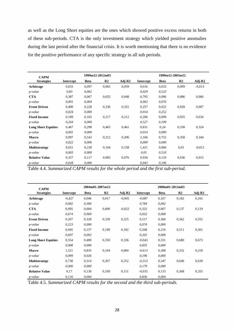
The results for unconditional CAPM indicate that except for the last period, the majority of

the hedge funds strategies provided abnormal returns throughout the investigation. During the

whole period almost all the investment styles but arbitrage and fixed income, yielded positive

excess returns with regard to their significant positive Jensen’s alpha. In the first sub period,

excluding Fixed Income, all the strategies show significant positive intercept at level of 5

percent. In the second sub period only three strategies gained positive abnormal returns

whereas the Arbitrage strategy provided negative significant Jensen’s alpha. Multi-strategies

28

as well as the Long Short equities are the ones which showed positive excess returns in both

of these sub-periods. CTA is the only investment strategy which yielded positive anomalies

during the last period after the financial crisis. It is worth mentioning that there is no evidence

for the positive performance of any specific strategy in all sub periods.

CAPM

Strategies

1999m12-2012m03 1999m12-2003m12

Intercept Beta R2 Adj-R2 Intercept Beta R2 Adj-R2

Arbitrage 0,033 0,097 0,065 0,059 0,616 0,033 0,009 -0,013

p-value 0,83 0,002

0,029 0,523

CTA 0,387 0,067 0,055 0,048 0,795 0,096 0,086 0,066

p-value 0,001 0,004

0,002 0,076

Event Driven 0,400 0,228 0,336 0,331 0,257 0,022 0,028 0,007

p-value 0,024 0,000

0,014 0,252

Fixed Income 0,189 0,165 0,217 0,212 0,206 0,099 0,055 0,034

p-value 0,264 0,000

0,527 0,109

Long Short Equities 0,467 0,298 0,465 0,461 0,831 0,24 0,338 0,324

p-value 0,001 0,000

0,014 0,000

Macro 0,997 0,543 0,212 0,206 2,166 0,752 0,358 0,344

p-value 0,022 0,000

0,009 0,000

Multistrategy 0,651 0,228 0,164 0,158 1,421 0,066 0,01 -0,012

p-value 0,003 0,000

0,01 0,510

Relative Value 0,357 0,117 0,083 0,076 0,934 0,110 0,036 0,015

p-value 0,028 0,000 0,043 0,196

Table 4.4. Summarized CAPM results for the whole period and the first sub-period.

CAPM

Strategies

2004m01-2007m12 2008m01-2012m03

Intercept Beta R2 Adj-R2 Intercept Beta R2 Adj-R2

Arbitrage -0,427 0,046 0,017 -0,005 -0,087 0,167 0,182 0,165

p-value 0,002 0,384

0,784 0,002

CTA 0,095 0,004 0,000 -0,022 0,332 0,067 0,137 0,119

p-value 0,674 0,969

0,032 0,008

Event Driven 0,207 0,328 0,339 0,325 0,517 0,360 0,562 0,552

p-value 0,223 0,000

0,076 0,000

Fixed Income 0,045 0,157 0,199 0,182 0,268 0,216 0,511 0,501

p-value 0,697 0,002

0,202 0,000

Long Short Equities 0,554 0,400 0,350 0,336 -0,043 0,331 0,680 0,673

p-value 0,008 0,000

0,835 0,000

Macro 1,521 0,835 0,104 0,084 -0,613 0,368 0,332 0,318

p-value 0,099 0,026

0,196 0,000

Multistrategy 0,738 0,314 0,267 0,252 -0,313 0,347 0,646 0,639

p-value 0,000 0,000

0,179 0,000

Relative Value 0,17 0,130 0,169 0,151 -0,035 0,133 0,368 0,355

p-value 0,116 0,004 0,836 0,004

Table 4.5. Summarized CAPM results for the second and the third sub-periods.

29

For the whole period as well as all the three sub-periods Macro strategy yielded the highest

abnormal return, however for the last period the alpha is not significant. The observed alphas

were not significant for Fixed Income strategy in any sub-period even at 10 percent

significance level. The alphas vary across strategies from 0.2% to almost 2% throughout the

different sub-periods. Event driven yielded the lowest abnormal return of 0.25 percent per

month in the first period while the highest anomaly provided by Macro (2.16 percent) for the

same duration of time.

It is logical to expect very low betas for hedge fund returns, since by definition the

performance of these funds should be independent of the market movements. However,

obtaining factor loadings close to zero is unlikely in reality. Except for the first sub-period,

nearly all the betas are significant for all the investment styles. The beta differs from 0.066 for

CTA in the last sub period to 0.83 for Macro in the second sub-period. Throughout the entire

period the results didn’t show any negative factor loadings for any of the strategies.

According to R2 and adjusted-R

2, it seems that unconditional one factor asset pricing model,

CAPM is incapable of explaining the performance of the hedge fund returns. The values for

adjusted-R2 vary from -0.021 for CTA in the second period to 0.673 for Long Short equities

in the third period. It can be concluded that highest adjusted-R2 is obtainable for strategies

that are highly related to the equity market. However, in general low goodness of fit results

indicates the poor explanatory power of the model. CAPM doesn’t allow for inclusion of

other risk factors in the model so is not appropriate to capture the variability of returns of the

different of hedge funds.

4.3 Fama-French Three Factor Model

Secondly, we are interested in investigating another static model, named Fama-French three

factor model which have proven to outperform CAPM as it additionally includes both size-

and book-to-market risk factors. As presented in 2.6.2, we estimate the following equation:

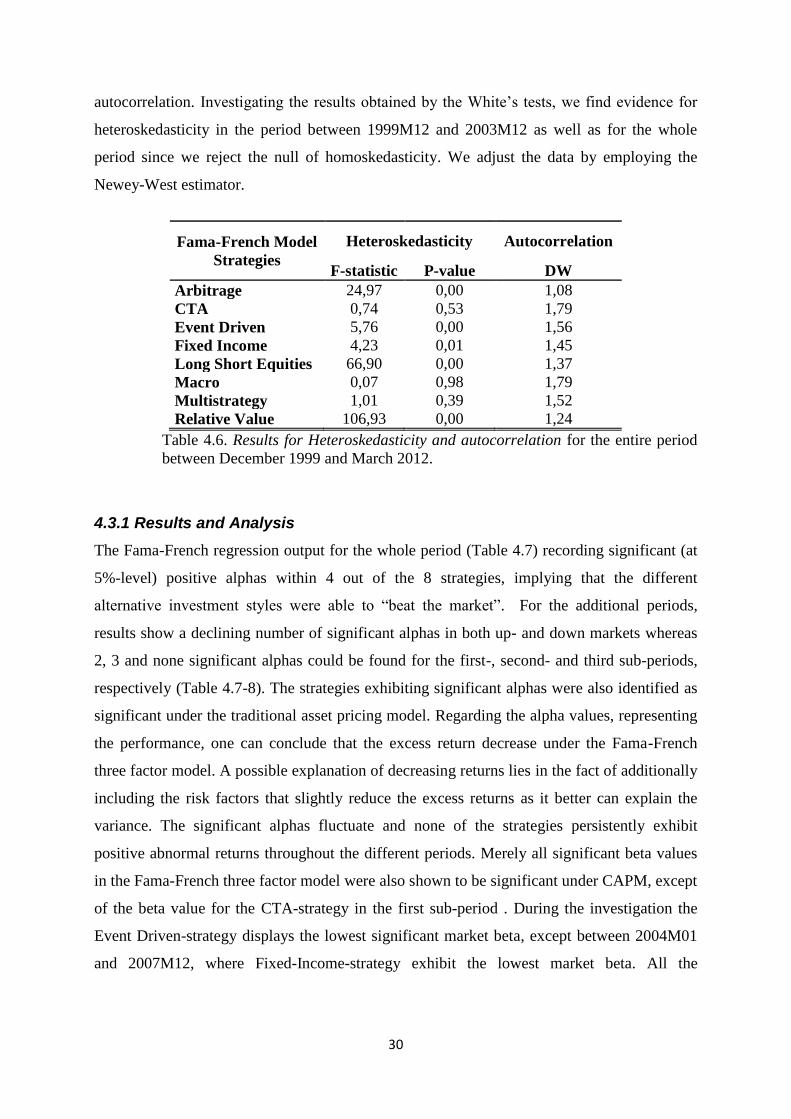
Whilst estimating the equation, tests results from the DW and White’s-test implies that some

regressions suffer from both autocorrelation and heteroskedasticity (see Table 4.6, Appendix:

Table 7.6). Examining the Durbin-Watson statistics, we conclude that only arbitrage strategy,

in the period between 1999M12 and 2003M12, demonstrate problems related to

30

autocorrelation. Investigating the results obtained by the White’s tests, we find evidence for

heteroskedasticity in the period between 1999M12 and 2003M12 as well as for the whole

period since we reject the null of homoskedasticity. We adjust the data by employing the

Newey-West estimator.

Fama-French Model

Strategies

Heteroskedasticity Autocorrelation

F-statistic P-value DW

Arbitrage 24,97 0,00 1,08

CTA 0,74 0,53 1,79

Event Driven 5,76 0,00 1,56

Fixed Income 4,23 0,01 1,45

Long Short Equities 66,90 0,00 1,37

Macro 0,07 0,98 1,79

Multistrategy 1,01 0,39 1,52

Relative Value 106,93 0,00 1,24

Table 4.6. Results for Heteroskedasticity and autocorrelation for the entire period

between December 1999 and March 2012.

4.3.1 Results and Analysis

The Fama-French regression output for the whole period (Table 4.7) recording significant (at

5%-level) positive alphas within 4 out of the 8 strategies, implying that the different

alternative investment styles were able to “beat the market”. For the additional periods,

results show a declining number of significant alphas in both up- and down markets whereas

2, 3 and none significant alphas could be found for the first-, second- and third sub-periods,

respectively (Table 4.7-8). The strategies exhibiting significant alphas were also identified as

significant under the traditional asset pricing model. Regarding the alpha values, representing

the performance, one can conclude that the excess return decrease under the Fama-French

three factor model. A possible explanation of decreasing returns lies in the fact of additionally

including the risk factors that slightly reduce the excess returns as it better can explain the

variance. The significant alphas fluctuate and none of the strategies persistently exhibit

positive abnormal returns throughout the different periods. Merely all significant beta values

in the Fama-French three factor model were also shown to be significant under CAPM, except

of the beta value for the CTA-strategy in the first sub-period . During the investigation the

Event Driven-strategy displays the lowest significant market beta, except between 2004M01

and 2007M12, where Fixed-Income-strategy exhibit the lowest market beta. All the

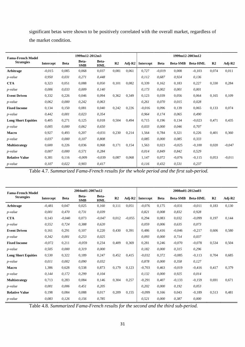
31

significant betas were shown to be positively correlated with the overall market, regardless of

the market condition.

Fama-French Model

Strategies

1999m12-2012m3 1999m12-2003m12

Intercept Beta Beta-

SMB

Beta-

HML R2 Adj-R2 Intercept Beta Beta-SMB Beta-HML R2 Adj-R2

Arbitrage -0,015 0,085 0,068 0,037 0,081 0,061 0,727 -0,019 0,008 -0,103 0,074 0,011

p-value 0,950 0,031 0,271 0,448

0,112 0,687 0,924 0,136

CTA 0,323 0,051 0,088 0,050 0,101 0,082 0,339 0,162 0,183 0,227 0,330 0,284

p-value 0,006 0,033 0,009 0,140

0,173 0,002 0,001 0,001

Event Driven 0,332 0,226 0,046 0,094 0,362 0,349 0,123 0,039 0,056 0,064 0,165 0,109

p-value 0,062 0,000 0,242 0,063

0,261 0,070 0,015 0,028

Fixed Income 0,134 0,150 0,081 0,040 0,242 0,226 -0,016 0,096 0,139 0,065 0,133 0,074

p-value 0,442 0,001 0,023 0,354

0,964 0,174 0,065 0,490

Long Short Equities 0,405 0,271 0,125 0,018 0,504 0,494 0,715 0,196 0,134 -0,023 0,471 0,435

p-value 0,005 0,000 0,062 0,650

0,033 0,000 0,046 0,707

Macro 0,927 0,493 0,207 -0,031 0,230 0,214 1,564 0,784 0,321 0,226 0,401 0,360

p-value 0,037 0,000 0,107 0,808

0,085 0,000 0,085 0,333

Multistrategy 0,600 0,226 0,036 0,068 0,171 0,154 1,563 0,023 -0,025 -0,100 0,020 -0,047

p-value 0,007 0,000 0,571 0,284

0,014 0,849 0,842 0,529

Relative Value 0,381 0,116 -0,009 -0,039 0,087 0,068 1,147 0,072 -0,076 -0,115 0,053 -0,011

p-value 0,107 0,022 0,903 0,417 0,116 0,432 0,531 0,237

Table 4.7. Summarized Fama-French results for the whole period and the first sub-period.

Fama-French Model

Strategies

2004m01-2007m12 2008m01-2012m03

Intercept Beta Beta-

SMB

Beta-

HML R2 Adj-R2 Intercept Beta Beta-SMB Beta-HML R2 Adj-R2

Arbitrage -0,481 0,047 0,025 0,160 0,111 0,051 -0,076 0,175 -0,031 -0,011 0,183 0,130

p-value 0,001 0,470 0,731 0,039

0,821 0,008 0,832 0,928

CTA 0,143 -0,040 0,073 -0,047 0,012 -0,055 0,294 0,083 0,032 -0,099 0,197 0,144

p-value 0,552 0,724 0,388 0,620

0,059 0,006 0,635 0,073

Event Driven 0,161 0,291 0,107 0,220 0,430 0,391 0,486 0,416 -0,046 -0,217 0,606 0,580

p-value 0,342 0,001 0,253 0,025

0,093 0,000 0,714 0,037

Fixed Income -0,072 0,211 -0,059 0,234 0,409 0,369 0,281 0,246 -0,070 -0,078 0,534 0,504

p-value 0,505 0,000 0,319 0,000

0,182 0,000 0,315 0,296

Long Short Equities 0,530 0,322 0,189 0,247 0,452 0,415 -0,032 0,372 -0,085 -0,113 0,704 0,685

p-value 0,011 0,002 0,090 0,032

0,878 0,000 0,358 0,127

Macro 1,386 0,628 0,538 0,873 0,179 0,123 -0,703 0,463 -0,019 -0,416 0,417 0,379

p-value 0,144 0,172 0,299 0,104

0,132 0,000 0,925 0,014

Multistrategy 0,713 0,283 0,084 0,146 0,304 0,257 -0,291 0,407 -0,133 -0,159 0,691 0,671

p-value 0,001 0,006 0,451 0,205

0,202 0,000 0,192 0,053

Relative Value 0,198 0,084 0,088 0,017 0,209 0,155 -0,099 0,166 0,043 -0,189 0,513 0,481

p-value 0,083 0,126 0,156 0,785 0,521 0,000 0,387 0,000

Table 4.8. Summarized Fama-French results for the second and the third sub-period.

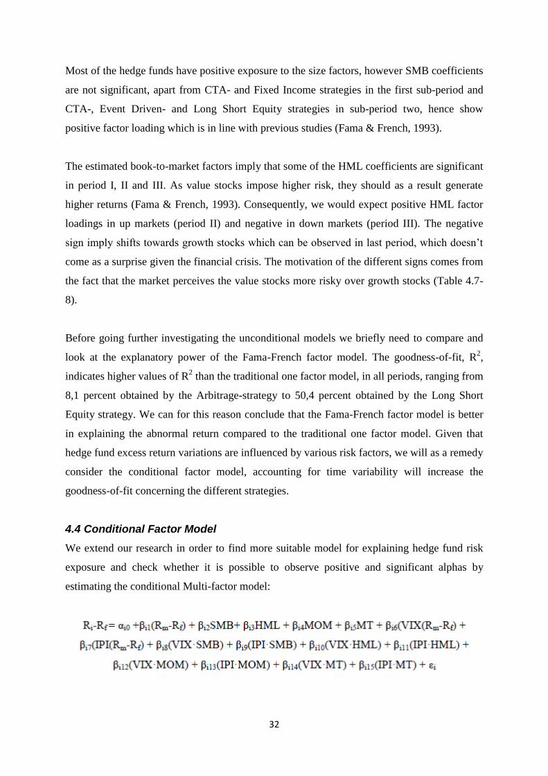
32

Most of the hedge funds have positive exposure to the size factors, however SMB coefficients

are not significant, apart from CTA- and Fixed Income strategies in the first sub-period and

CTA-, Event Driven- and Long Short Equity strategies in sub-period two, hence show

positive factor loading which is in line with previous studies (Fama & French, 1993).

The estimated book-to-market factors imply that some of the HML coefficients are significant

in period I, II and III. As value stocks impose higher risk, they should as a result generate

higher returns (Fama & French, 1993). Consequently, we would expect positive HML factor

loadings in up markets (period II) and negative in down markets (period III). The negative

sign imply shifts towards growth stocks which can be observed in last period, which doesn’t

come as a surprise given the financial crisis. The motivation of the different signs comes from

the fact that the market perceives the value stocks more risky over growth stocks (Table 4.7-

8).

Before going further investigating the unconditional models we briefly need to compare and

look at the explanatory power of the Fama-French factor model. The goodness-of-fit, R2,

indicates higher values of R2 than the traditional one factor model, in all periods, ranging from

8,1 percent obtained by the Arbitrage-strategy to 50,4 percent obtained by the Long Short

Equity strategy. We can for this reason conclude that the Fama-French factor model is better

in explaining the abnormal return compared to the traditional one factor model. Given that

hedge fund excess return variations are influenced by various risk factors, we will as a remedy

consider the conditional factor model, accounting for time variability will increase the

goodness-of-fit concerning the different strategies.

4.4 Conditional Factor Model

We extend our research in order to find more suitable model for explaining hedge fund risk

exposure and check whether it is possible to observe positive and significant alphas by

estimating the conditional Multi-factor model:

33

Hence, we extend the Fama-French three factor model, by adding the supplementary risk

factors, momentum and market timing. In addition we include instrumental variables that

incorporate market’s perception of risk, VIX, and the variable that stands as a proxy for the

overall market situation, IPI.

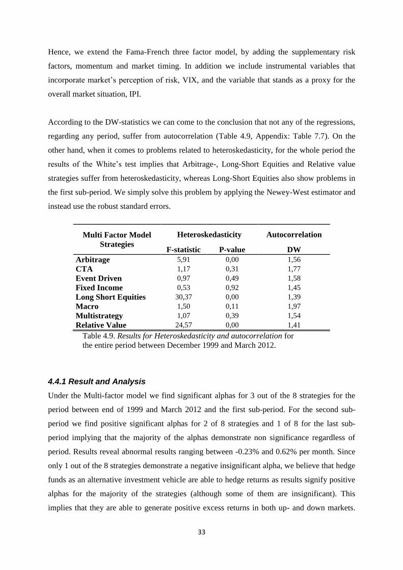
According to the DW-statistics we can come to the conclusion that not any of the regressions,

regarding any period, suffer from autocorrelation (Table 4.9, Appendix: Table 7.7). On the

other hand, when it comes to problems related to heteroskedasticity, for the whole period the

results of the White’s test implies that Arbitrage-, Long-Short Equities and Relative value

strategies suffer from heteroskedasticity, whereas Long-Short Equities also show problems in

the first sub-period. We simply solve this problem by applying the Newey-West estimator and

instead use the robust standard errors.

Multi Factor Model

Strategies

Heteroskedasticity Autocorrelation

F-statistic P-value DW

Arbitrage 5,91 0,00 1,56

CTA 1,17 0,31 1,77

Event Driven 0,97 0,49 1,58

Fixed Income 0,53 0,92 1,45

Long Short Equities 30,37 0,00 1,39

Macro 1,50 0,11 1,97

Multistrategy 1,07 0,39 1,54

Relative Value 24,57 0,00 1,41

Table 4.9. Results for Heteroskedasticity and autocorrelation for

the entire period between December 1999 and March 2012.

4.4.1 Result and Analysis

Under the Multi-factor model we find significant alphas for 3 out of the 8 strategies for the

period between end of 1999 and March 2012 and the first sub-period. For the second sub-

period we find positive significant alphas for 2 of 8 strategies and 1 of 8 for the last sub-

period implying that the majority of the alphas demonstrate non significance regardless of

period. Results reveal abnormal results ranging between -0.23% and 0.62% per month. Since

only 1 out of the 8 strategies demonstrate a negative insignificant alpha, we believe that hedge

funds as an alternative investment vehicle are able to hedge returns as results signify positive

alphas for the majority of the strategies (although some of them are insignificant). This

implies that they are able to generate positive excess returns in both up- and down markets.

34

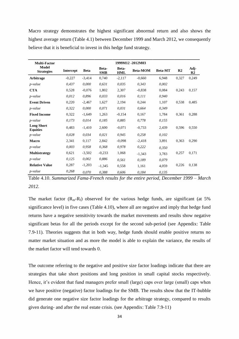
Macro strategy demonstrates the highest significant abnormal return and also shows the

highest average return (Table 4.1) between December 1999 and March 2012, we consequently

believe that it is beneficial to invest in this hedge fund strategy.

Multi-Factor

Model

Strategies

1999M12 -2012M03

Intercept Beta Beta-

SMB

Beta-

HML Beta-MOM Beta-MT R2

Adj-

R2

Arbitrage -0,227 -3,414 0,740 -2,117 -0,660 6,948 0,327 0,249

p-value 0,437 0,000 0,631 0,035 0,343 0,002

CTA 0,528 -0,076 1,802 2,307 -0,838 0,084 0,243 0,157

p-value 0,012 0,896 0,033 0,016 0,111 0,940

Event Driven 0,220 -2,467 1,627 2,194 0,244 1,107 0,538 0,485

p-value 0,322 0,000 0,071 0,031 0,664 0,349

Fixed Income 0,322 -1,649 1,263 -0,154 0,167 1,784 0,361 0,288

p-value 0,173 0,014 0,185 0,885 0,778 0,155

Long Short

Equities 0,483 -1,410 2,600 -0,071 -0,733 2,439 0,596 0,550

p-value 0,028 0,034 0,021 0,945 0,258 0,102

Macro 2,341 0,117 2,842 -0,098 -2,418 3,891 0,363 0,290

p-value 0,003 0,958 0,368 0,978 0,222 0,350 Multistrategy 0,621 -3,502 -0,233 1,068 -1,343 3,783 0,257 0,171

p-value 0,125 0,002 0,886 0,561 0,189 0,079 Relative Value 0,287 -1,203 -1,345 0,558 1,161 4,059 0,226 0,138

p-value 0,268 0,070 0,388 0,606 0,184 0,135

Table 4.10. Summarized Fama-French results for the entire period, December 1999 – March

2012.

The market factor (Rm-Rf) observed for the various hedge funds, are significant (at 5%

significance level) in five cases (Table 4.10), where all are negative and imply that hedge fund

returns have a negative sensitivity towards the market movements and results show negative

significant betas for all the periods except for the second sub-period (see Appendix: Table

7.9-11). Theories suggests that in both way, hedge funds should enable positive returns no

matter market situation and as more the model is able to explain the variance, the results of

the market factor will tend towards 0.

The outcome referring to the negative and positive size factor loadings indicate that there are

strategies that take short positions and long position in small capital stocks respectively.

Hence, it’s evident that fund managers prefer small (large) caps over large (small) caps when

we have positive (negative) factor loadings for the SMB. The results show that the IT-bubble

did generate one negative size factor loadings for the arbitrage strategy, compared to results

given during- and after the real estate crisis. (see Appendix: Table 7.9-11)

35

Three out of the eight HML coefficients are significant (Table 4.10), whereas two of the

strategies show positive factor loadings. We cannot therefore explain whether hedge funds are

exposed to value risk and if preferences lean towards growth stocks, since only two of the all

show positive factor loadings.

Data sample stretching between December 1999 and March 2012 show that none of strategies

demonstrate significant momentum beta. Referring to period I and II we find that 1 and for

period III, 3 out of 8 strategies respectively show significant betas. On the other hand the sign

does vary, where the majority of the strategies show negative significant betas for the period

II and III, implying that momentum cannot be considered as a compensation of bearing an

extra risk, i.e. momentum can’t explain the abnormal returns.

Regarding the market timing ability, MT, the results show that only one out of all the

strategies (Arbitrage) in the whole period shows significant coefficient value while we get

positive significant betas for 3 and 2 of the strategies for the first and third sub-periods

respectively (see Table 4.10, Appendix: Table 7.9-11). The existence of positive market

timing ability is in line with Chen and Liang (2007). Meaning that, hedge fund managers in

deed are able to earn higher abnormal returns when the market is expected to rise, which is in

line with Gupta et al. (2003). However, according to our findings the small number of

significant coefficients implies that this cannot be verified.

The conditional effects in Table 7.8 (see Appendix) shows that the (IPI·Rm-Rf) is positive and

for the majority also significant. This implies that the market factor is higher in bear markets,

i.e. the hedge funds will follow the market more in up markets and less in down markets,

which seems logical. For the other conditional effects, a minor part of the betas are not

significant and for this reason we are not able to explain the various conditioning effects.

The goodness-of-fit, R2

and the adjusted-R2 of the conditional Multi-factor model indicates

that the explanatory power is significantly higher than for both CAPM and Fama-French three

factor model. The explanatory power has consistently risen, varying from 22% and 60%, the

results proves that the conditional Multi-factor model, including both additional risk factors

and instrumental variables provides the best fit compared to the static models, as it

significantly and consistent contribute to the models explanatory power.

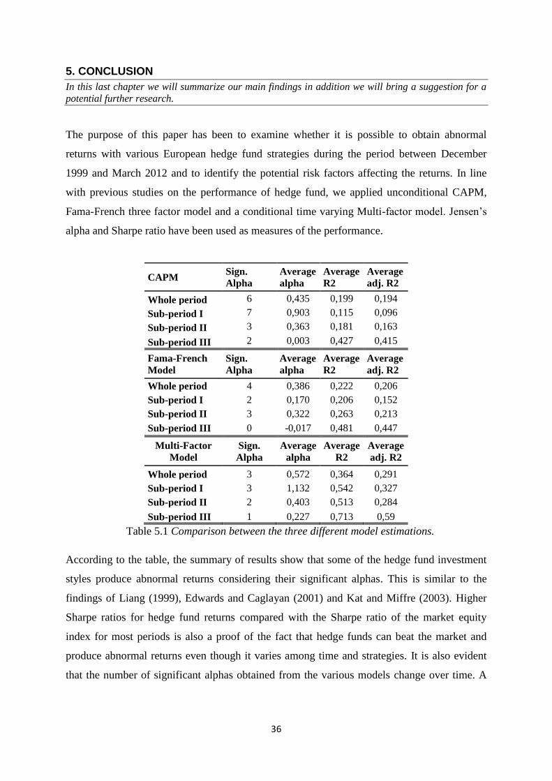
36

5. CONCLUSION

In this last chapter we will summarize our main findings in addition we will bring a suggestion for a

potential further research.

The purpose of this paper has been to examine whether it is possible to obtain abnormal

returns with various European hedge fund strategies during the period between December

1999 and March 2012 and to identify the potential risk factors affecting the returns. In line

with previous studies on the performance of hedge fund, we applied unconditional CAPM,

Fama-French three factor model and a conditional time varying Multi-factor model. Jensen’s

alpha and Sharpe ratio have been used as measures of the performance.

CAPM Sign.

Alpha

Average

alpha

Average

R2

Average

adj. R2

Whole period 6 0,435 0,199 0,194

Sub-period I 7 0,903 0,115 0,096

Sub-period II 3 0,363 0,181 0,163

Sub-period III 2 0,003 0,427 0,415

Fama-French

Model

Sign.

Alpha

Average

alpha

Average

R2

Average

adj. R2

Whole period 4 0,386 0,222 0,206

Sub-period I 2 0,170 0,206 0,152

Sub-period II 3 0,322 0,263 0,213

Sub-period III 0 -0,017 0,481 0,447

Multi-Factor

Model

Sign.

Alpha

Average

alpha

Average

R2

Average

adj. R2

Whole period 3 0,572 0,364 0,291

Sub-period I 3 1,132 0,542 0,327

Sub-period II 2 0,403 0,513 0,284

Sub-period III 1 0,227 0,713 0,59

Table 5.1 Comparison between the three different model estimations.

According to the table, the summary of results show that some of the hedge fund investment

styles produce abnormal returns considering their significant alphas. This is similar to the

findings of Liang (1999), Edwards and Caglayan (2001) and Kat and Miffre (2003). Higher

Sharpe ratios for hedge fund returns compared with the Sharpe ratio of the market equity

index for most periods is also a proof of the fact that hedge funds can beat the market and

produce abnormal returns even though it varies among time and strategies. It is also evident

that the number of significant alphas obtained from the various models change over time. A

37

possible explanation could be due to the fact that manager’s ability to earn hedge fund returns

differs among various business cycles.

The goodness-of-fit consistently rise as we include additional explanatory variables to the

model, which was expected. R2

and adjusted-R2

show lower values for the CAPM and Fama-

French compared to the conditional Multi-factor model. Hence, both models appear to be

inappropriate to capture the performance of hedge funds as they are not able to explain the

dynamic risk exposures. Even thought the average goodness-of-fit of the conditional model is

not as high as we expected, it is still higher than 35 percent reported by Kat and Miffre

(2003). Another explanation of the poor goodness-of-fit can be attributed to the number of

explanatory variables and including insufficient risk factors.

5.1 Further studies

We believe that it could be a matter of interest to include supplementary risk factors as well as

instrumental variables as a proxy for the business cycles in order to enhance the explanation

power of the Multi-factor model. Furthermore, including other strategies as well as a more

specified group of countries such as eastern or western European countries would be relevant

to explore the existence of abnormal returns in the European markets.

38

6. REFERENCES

Ackermann C., McEnally R., Ravenskraft D. (1999) The Performance of Hedge Funds: Risk,

Return and Insentives. Journal of Finance, Vol.54, No. 3, 833-874.

Agarwal, V., Naik, N. (2000). Multi-Period Performance Persistence Analysis of Hedge

Funds. The Journal of Financial and Quantitative Analysis, Vol. 35, No. 3, 327-342.

Anderlind, P., Eidolf, E., Holm, M., Sommerlau, P. (2003). Hedgefonder. Academia Adacta,

Lund

Brooks, C. (2008). Introductory Econometrics for Finance. Cambridge University Press.

Brown, S. J., Goetzmann W. N., & Ibbotson R. G. (1999). Offshore Hedgefunds: Survival and

Performance 1989-1995. Journal of Business, Vol. 72, No. 1, 91-117.

Carhart M.M. (1997). On Persistence in Mutual Fund Performance. The Journal of Finance,

Vol.52, No 1, 57-82.

Campbell, J.Y., Lo, A.W. & Mackinlay, A.C. (1997). The Econometrics of Financial Markets.

Princeton University Press.

Chen, Y., & Liang, B., (2007). Do Market Timing Hedge Funds time the market?

Journal of Financial and Quantitative Analysis, Vol. 42, No. 2, 827-856.

Connor, G. & Korajczyk, R., (1988). Risk and Return in an Equilibrium APT: Application of

a New Test Methodology. Journal of Financial Economics, Vol. 21, 255-290.

Durbin, J., & Watson, G. S., (1951). Testing for Serial Correlation in Least Squares

Regression, II. Biometrika, Vol. 38, 159–179.

Edwards, F., & Caglayan, M., (2001). Hedge Fund Performance and Manager Skill. Journal

of Futures Markets, Vol. 21, No.11, 1003-1028

39

Fama, E., & French, K. (1993). Common Risk Factors in the Returns on Stocks and Bonds.

Journal of Financial Economics, 33, 3-56.

Fama, E.F. & French, K.R. (1996). Multifactor Explanations of Asset Pricing Anomalies. The

Journal of Finance, Vol. 51, No. 1, 55-84.

Ferson, W., & Harvey C. (1999). Conditioning Variables and the Cross Section of Stock

Returns. The Journal of Finance, Vol. 4, 132-135.

Ferson, W., & Schadt, R. (1996). Measuring Fund Strategy and Performance in Changing

Economic Conditions. Journal of Finance, Vol. 51, 425-462.

Fung, W., Hsieh, D. A. (1997a). Emprical Characteristics of Dynamic Trading Strategies: The

Case of Hedge Funds. Review of Financial Studies, Vol. 10, 275-302.

Fung, W., Hsieh, D. A. (2000). Performance characteristics of hedge funds and commodity

funds: Natural vs. spurious biases. Journal of Financial and Quantitative Analysis, Vol. 35,

291–307.

Fung, H.G., Xu, X.E., & Yau, J., (2002). Global Hedge Funds: Risk, Return and Market

Timing. Financial Analysts Journal, Vol. 58, No. 6, 19-30.

Gujarati, D. (2006). Essentials of Econometrics (3rd ed.). Singapore: McGraw-Hill.

Gupta, B., Cerrahoglu, B., & Daglioglu, A. (2003). Evaluating Hedge Fund Performance:

Traditional Versus Conditional Approach. The Journal of Alternative Investments, 7-24.

Jacobsen, D. I., (2002). Vad, hur och varför? Om metodval i företagsekonomi och andra

samhällsvetenskapliga ämnen. Studentlitteratur: Lund.

Jegadeesh, N. &Titman, S. (1993). Returns to Buying Winners and Selling Losers:

Implications for Market Efficiency. Journal of Finance, Vol. 48, 35-91.

40

Kat, H. M., & Miffre, J. (2003). Performance Evaluation and Conditioning Information:

The Case of Hedge Funds, Working paper. Faculty of Finance, Cass Business School, London

Lehmann, B. & Modest, D. (1988). The Empirical Foundations of the Arbitrage Pricing

Theory. Journal of Financial Economics, Vol. 21, 213-254.

Liang, B. (1999). On the Performance of Hedge Funds. Financial Analysts Journal, Vol. 55,

No. 4, 72-85.

Liew, J. & M. Vassalou (2000). Can book-to-market, size, and momentum be risk factors that

predict economic growth? Journal of Financial Economics 57, 221–245.

Malkiel, B., & Saha, A. (2005). Hedge Funds: Risk and Return. Financial Analysts Journal,

Vol. 61, No. 6, 80-88.

Ogden, J.P., Jen, F.C. & O’Connor, P.F. (2002). Advanced Corporate Finance – Policies and

Strategies. Prentice Hall.

Whaley, R.E. (2000). The investor fear gauge. Journal of Portfolio Management, Vol. 26, 12-

17.

White, H. (1980). A Heteroskedasticity-Consistent Covariance Matrix Estimator and a Direct

Test for Heteroskedasticity. Econometrica, Vol. 48, 817-38.

DATA SOURCES

Eureka Hedge homepage: Indices. Available at: http://eurekahedge.com/indices/default.asp.

(Accessed: 25th

April, 2012).

Kenneth, R. French homepage: Data library – Fama/French Factors (including momentum).

Available at: http://mba.tuck.dartmouth.edu/pages/faculty/ken.french/data_library.html.

(Accessed: 25th

April, 2012).

41

Datastream Advance Database, Thomson Financial Ltd. (MOM, MT, VIX, IPI, S&P Europe

350). (Accessed: 30th

May, 2012).

INTERNET SOURCES

The Hedge Fund Association. Retrieved from: https://thehfa.org/aboutus, (2012-04-20).

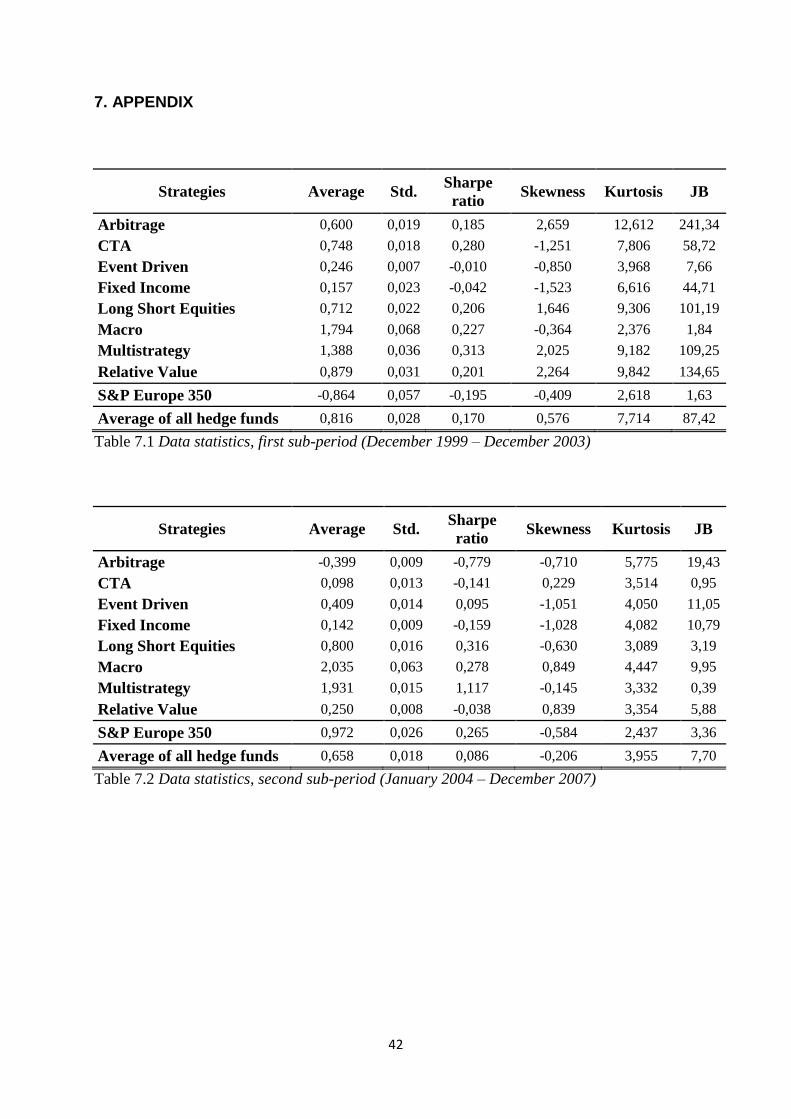
42

7. APPENDIX

Strategies Average Std. Sharpe

ratio Skewness Kurtosis JB

Arbitrage 0,600 0,019 0,185 2,659 12,612 241,34

CTA 0,748 0,018 0,280 -1,251 7,806 58,72

Event Driven 0,246 0,007 -0,010 -0,850 3,968 7,66

Fixed Income 0,157 0,023 -0,042 -1,523 6,616 44,71

Long Short Equities 0,712 0,022 0,206 1,646 9,306 101,19

Macro 1,794 0,068 0,227 -0,364 2,376 1,84

Multistrategy 1,388 0,036 0,313 2,025 9,182 109,25

Relative Value 0,879 0,031 0,201 2,264 9,842 134,65

S&P Europe 350 -0,864 0,057 -0,195 -0,409 2,618 1,63

Average of all hedge funds 0,816 0,028 0,170 0,576 7,714 87,42

Table 7.1 Data statistics, first sub-period (December 1999 – December 2003)

Strategies Average Std. Sharpe

ratio Skewness Kurtosis JB

Arbitrage -0,399 0,009 -0,779 -0,710 5,775 19,43

CTA 0,098 0,013 -0,141 0,229 3,514 0,95

Event Driven 0,409 0,014 0,095 -1,051 4,050 11,05

Fixed Income 0,142 0,009 -0,159 -1,028 4,082 10,79

Long Short Equities 0,800 0,016 0,316 -0,630 3,089 3,19

Macro 2,035 0,063 0,278 0,849 4,447 9,95

Multistrategy 1,931 0,015 1,117 -0,145 3,332 0,39

Relative Value 0,250 0,008 -0,038 0,839 3,354 5,88

S&P Europe 350 0,972 0,026 0,265 -0,584 2,437 3,36

Average of all hedge funds 0,658 0,018 0,086 -0,206 3,955 7,70

Table 7.2 Data statistics, second sub-period (January 2004 – December 2007)

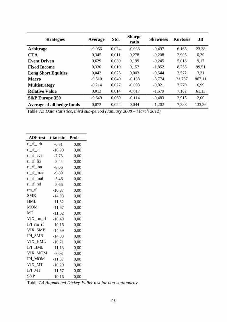
43

Strategies Average Std. Sharpe

ratio Skewness Kurtosis JB

Arbitrage -0,056 0,024 -0,038 -0,497 6,165 23,38

CTA 0,345 0,011 0,278 -0,208 2,905 0,39

Event Driven 0,629 0,030 0,199 -0,245 5,018 9,17

Fixed Income 0,330 0,019 0,157 -1,852 8,755 99,51

Long Short Equities 0,042 0,025 0,003 -0,544 3,572 3,21

Macro -0,510 0,040 -0,138 -3,774 21,737 867,11

Multistrategy -0,214 0,027 -0,093 -0,821 3,770 6,99

Relative Value 0,012 0,014 -0,017 -1,679 7,182 61,13

S&P Europe 350 -0,649 0,060 -0,114 -0,483 2,915 2,00

Average of all hedge funds 0,072 0,024 0,044 -1,202 7,388 133,86

Table 7.3 Data statistics, third sub-period (January 2008 – March 2012)

ADF-test t-tatistic Prob

ri_rf_arb -6,81 0,00

ri_rf_cta -10,90 0,00

ri_rf_eve -7,75 0,00

ri_rf_fix -8,44 0,00

ri_rf_lon -8,06 0,00

ri_rf_mac -9,89 0,00

ri_rf_mul -5,46 0,00

ri_rf_rel -8,66 0,00

rm_rf -10,37 0,00

SMB -14,08 0,00

HML -11,32 0,00

MOM -11,67 0,00

MT -11,62 0,00

VIX_rm_rf -10,49 0,00

IPI_rm_rf -10,16 0,00

VIX_SMB -14,59 0,00

IPI_SMB -14,03 0,00

VIX_HML -10,71 0,00

IPI_HML -11,13 0,00

VIX_MOM -7,03 0,00

IPI_MOM -11,57 0,00

VIX_MT -10,20 0,00

IPI_MT -11,57 0,00

S&P -10,16 0,00

Table 7.4 Augmented Dickey-Fuller test for non-stationarity.

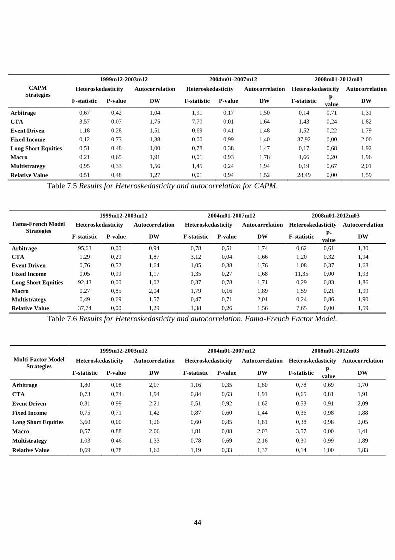
44

CAPM

Strategies

1999m12-2003m12 2004m01-2007m12 2008m01-2012m03

Heteroskedasticity Autocorrelation Heteroskedasticity Autocorrelation Heteroskedasticity Autocorrelation

F-statistic P-value DW F-statistic P-value DW F-statistic P-

value DW

Arbitrage 0,67 0,42 1,04 1,91 0,17 1,50 0,14 0,71 1,31

CTA 3,57 0,07 1,75 7,70 0,01 1,64 1,43 0,24 1,82

Event Driven 1,18 0,28 1,51 0,69 0,41 1,48 1,52 0,22 1,79

Fixed Income 0,12 0,73 1,38 0,00 0,99 1,40 37,92 0,00 2,00

Long Short Equities 0,51 0,48 1,00 0,78 0,38 1,47 0,17 0,68 1,92

Macro 0,21 0,65 1,91 0,01 0,93 1,78 1,66 0,20 1,96

Multistrategy 0,95 0,33 1,56 1,45 0,24 1,94 0,19 0,67 2,01

Relative Value 0,51 0,48 1,27 0,01 0,94 1,52 28,49 0,00 1,59

Table 7.5 Results for Heteroskedasticity and autocorrelation for CAPM.

Table 7.6 Results for Heteroskedasticity and autocorrelation, Fama-French Factor Model.

Fama-French Model

Strategies

1999m12-2003m12 2004m01-2007m12 2008m01-2012m03

Heteroskedasticity Autocorrelation Heteroskedasticity Autocorrelation Heteroskedasticity Autocorrelation

F-statistic P-value DW F-statistic P-value DW F-statistic P-

value DW

Arbitrage 95,63 0,00 0,94 0,78 0,51 1,74 0,62 0,61 1,30

CTA 1,29 0,29 1,87 3,12 0,04 1,66 1,20 0,32 1,94

Event Driven 0,76 0,52 1,64 1,05 0,38 1,76 1,08 0,37 1,68

Fixed Income 0,05 0,99 1,17 1,35 0,27 1,68 11,35 0,00 1,93

Long Short Equities 92,43 0,00 1,02 0,37 0,78 1,71 0,29 0,83 1,86

Macro 0,27 0,85 2,04 1,79 0,16 1,89 1,59 0,21 1,99

Multistrategy 0,49 0,69 1,57 0,47 0,71 2,01 0,24 0,86 1,90

Relative Value 37,74 0,00 1,29 1,38 0,26 1,56 7,65 0,00 1,59

Multi-Factor Model

Strategies

1999m12-2003m12 2004m01-2007m12 2008m01-2012m03

Heteroskedasticity Autocorrelation Heteroskedasticity Autocorrelation Heteroskedasticity Autocorrelation

F-statistic P-value DW F-statistic P-value DW F-statistic P-

value DW

Arbitrage 1,80 0,08 2,07 1,16 0,35 1,80 0,78 0,69 1,70

CTA 0,73 0,74 1,94 0,84 0,63 1,91 0,65 0,81 1,91

Event Driven 0,31 0,99 2,21 0,51 0,92 1,62 0,53 0,91 2,09

Fixed Income 0,75 0,71 1,42 0,87 0,60 1,44 0,36 0,98 1,88

Long Short Equities 3,60 0,00 1,26 0,60 0,85 1,81 0,38 0,98 2,05

Macro 0,57 0,88 2,06 1,81 0,08 2,03 3,57 0,00 1,41

Multistrategy 1,03 0,46 1,33 0,78 0,69 2,16 0,30 0,99 1,89

Relative Value 0,69 0,78 1,62 1,19 0,33 1,37 0,14 1,00 1,83

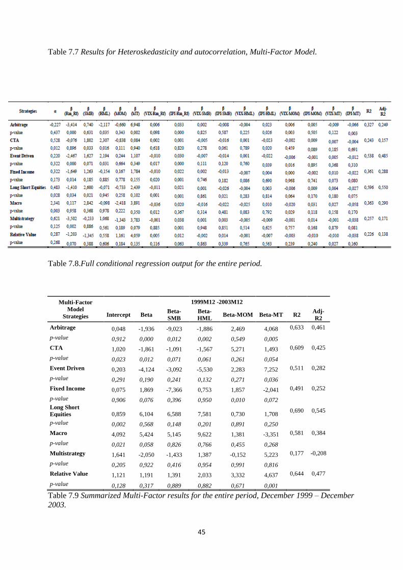
45

Table 7.7 Results for Heteroskedasticity and autocorrelation, Multi-Factor Model.

Table 7.8.Full conditional regression output for the entire period.

Multi-Factor

Model

Strategies

1999M12 -2003M12

Intercept Beta Beta-

SMB

Beta-

HML Beta-MOM Beta-MT R2

Adj-

R2

Arbitrage 0,048 -1,936 -9,023 -1,886 2,469 4,068 0,633 0,461

p-value 0,912 0,000 0,012 0,002 0,549 0,005 CTA 1,020 -1,861 -1,091 -1,567 5,271 1,493 0,609 0,425

p-value 0,023 0,012 0,071 0,061 0,261 0,054 Event Driven 0,203 -4,124 -3,092 -5,530 2,283 7,252 0,511 0,282

p-value 0,291 0,190 0,241 0,132 0,271 0,036 Fixed Income 0,075 1,869 -7,366 0,753 1,857 -2,041 0,491 0,252

p-value 0,906 0,076 0,396 0,950 0,010 0,072 Long Short

Equities 0,859 6,104 6,588 7,581 0,730 1,708 0,690 0,545

p-value 0,002 0,568 0,148 0,201 0,891 0,250 Macro 4,092 5,424 5,145 9,622 1,381 -3,351 0,581 0,384

p-value 0,021 0,058 0,826 0,766 0,455 0,268 Multistrategy 1,641 -2,050 -1,433 1,387 -0,152 5,223 0,177 -0,208

p-value 0,205 0,922 0,416 0,954 0,991 0,816 Relative Value 1,121 1,191 1,391 2,033 3,332 4,637 0,644 0,477

p-value 0,128 0,317 0,889 0,882 0,671 0,001

Table 7.9 Summarized Multi-Factor results for the entire period, December 1999 – December

2003.

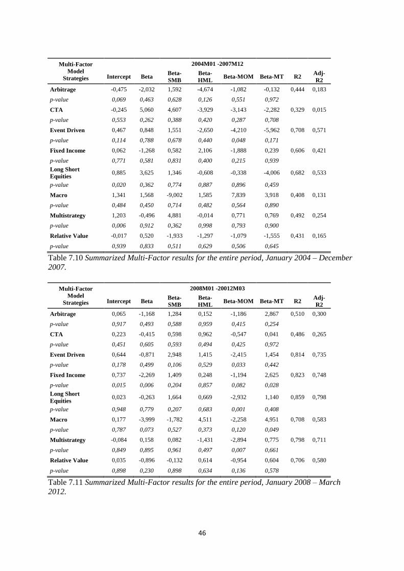
46

Multi-Factor

Model

Strategies

2004M01 -2007M12

Intercept Beta Beta-

SMB

Beta-

HML Beta-MOM Beta-MT R2

Adj-

R2

Arbitrage -0,475 -2,032 1,592 -4,674 -1,082 -0,132 0,444 0,183

p-value 0,069 0,463 0,628 0,126 0,551 0,972

CTA -0,245 5,060 4,607 -3,929 -3,143 -2,282 0,329 0,015

p-value 0,553 0,262 0,388 0,420 0,287 0,708

Event Driven 0,467 0,848 1,551 -2,650 -4,210 -5,962 0,708 0,571

p-value 0,114 0,788 0,678 0,440 0,048 0,171

Fixed Income 0,062 -1,268 0,582 2,106 -1,888 0,239 0,606 0,421

p-value 0,771 0,581 0,831 0,400 0,215 0,939

Long Short

Equities 0,885 3,625 1,346 -0,608 -0,338 -4,006 0,682 0,533

p-value 0,020 0,362 0,774 0,887 0,896 0,459

Macro 1,341 1,568 -9,002 1,585 7,839 3,918 0,408 0,131

p-value 0,484 0,450 0,714 0,482 0,564 0,890

Multistrategy 1,203 -0,496 4,881 -0,014 0,771 0,769 0,492 0,254

p-value 0,006 0,912 0,362 0,998 0,793 0,900

Relative Value -0,017 0,520 -1,933 -1,297 -1,079 -1,555 0,431 0,165

p-value 0,939 0,833 0,511 0,629 0,506 0,645

Table 7.10 Summarized Multi-Factor results for the entire period, January 2004 – December

2007.

Multi-Factor

Model

Strategies

2008M01 -20012M03

Intercept Beta Beta-

SMB

Beta-

HML Beta-MOM Beta-MT R2

Adj-

R2

Arbitrage 0,065 -1,168 1,284 0,152 -1,186 2,867 0,510 0,300

p-value 0,917 0,493 0,588 0,959 0,415 0,254

CTA 0,223 -0,415 0,598 0,962 -0,547 0,041 0,486 0,265

p-value 0,451 0,605 0,593 0,494 0,425 0,972

Event Driven 0,644 -0,871 2,948 1,415 -2,415 1,454 0,814 0,735

p-value 0,178 0,499 0,106 0,529 0,033 0,442

Fixed Income 0,737 -2,269 1,409 0,248 -1,194 2,625 0,823 0,748

p-value 0,015 0,006 0,204 0,857 0,082 0,028

Long Short

Equities 0,023 -0,263 1,664 0,669 -2,932 1,140 0,859 0,798

p-value 0,948 0,779 0,207 0,683 0,001 0,408

Macro 0,177 -3,999 -1,782 4,511 -2,258 4,951 0,708 0,583

p-value 0,787 0,073 0,527 0,373 0,120 0,049

Multistrategy -0,084 0,158 0,082 -1,431 -2,894 0,775 0,798 0,711

p-value 0,849 0,895 0,961 0,497 0,007 0,661

Relative Value 0,035 -0,896 -0,132 0,614 -0,954 0,604 0,706 0,580

p-value 0,898 0,230 0,898 0,634 0,136 0,578

Table 7.11 Summarized Multi-Factor results for the entire period, January 2008 – March

2012.