PERFORMANCE OF LARGE SCALE STEEL FIBER REINFORCED

CONCRETE DEEP BEAM WITH SINGLE OPENING

UNDER MONOTONIC LOADING

by

CARLOS A. FLORES

Presented to the Faculty of the Graduate School of

The University of Texas at Arlington in Partial Fulfillment

of the Requirements

for the Degree of

MASTER OF SCIENCE IN CIVIL ENGINEERING

The University of Texas at Arlington

August 2009

Copyright © by Carlos Flores 2009

All Rights Reserved

iii

ACKNOWLEDGEMENTS

I would like to express my sincere appreciation to my research advisor, Dr. Shih-Ho

Chao. Dr. Chao was persistent from the projects’ inception, giving priceless advice on ideas and

critiquing. I would also like to thank Dr. Guillermo Ramirez and Dr. John Matthys for their

patience with me and in providing ideas and advice on the research project. I would also like to

thank Hanson Pipe and Precast, Grand Prairie, TX, who donated materials for the test

specimen. I would like to thank Jae-sung Cho, Netra Karki, Reza Mohammed, who where

invaluable aid in the lab in this project. Finally, I would like to thank all the support staff at from

the Department of Civil and Environmental Engineering at The University of Texas at Arlington.

Without their continued support this project would never had been possible.

July 27, 2009

iv

ABSTRACT

PERFORMANCE OF LARGE SCALE STEEL FIBER REINFORCED

CONCRETE DEEP BEAM WITH SINGLE OPENING

UNDER MONOTONIC LOADING

Carlos Flores, M.S.

The University of Texas at Arlington, 2009

Supervising Professor: Shih-Ho Chao

The design of complex, discontinuous stress trajectory regions (D-regions) is complex

in nature and cumbersome to design. The performance of a large scale steel fiber reinforced

concrete (SFRC) deep beam with single opening under monotonic loading was tested under

controlled conditions. The main objective of this study was to see if Steel Fiber Reinforced

Concrete (SFRC), used as a better material than reinforced concrete (RC) offered an alternate

to the cumbersome and iterative steps involved in strut-and-tie (STM) methodology.

Additionally, a similar reinforced concrete (RC) specimen was tested under the same controlled

condition designed with classical strut-and-tie model design methodology reinforced using

conventional steel bars.

Material testing was conducted on the materials tested on the large scale specimens to

ensure that the actual material mechanical properties were known for the analysis. Computer

Aided Strut and Tie (CAST) software was used to quantify the experimental data obtained from

the controlled conditions testing.

v

The two beams were compared and contrasted throughout the study to indicate the

performance of one beam compared to the other. This study provides information on the

viability of using steel fiber reinforced concrete in complex D-regions in structural elements.

vi

TABLE OF CONTENTS

ACKNOWLEDGEMENTS .................................................................................................. iii ABSTRACT ........................................................................................................................ iv LIST OF ILLUSTRATIONS................................................................................................. ix LIST OF TABLES ............................................................................................................. xiv LIST OF NOTATIONS ..................................................................................................... xvi Chapter Page

1. INTRODUCTION ................................................................................................ 1

1.1 Introduction ............................................................................................. 1 1.2 Literature Review .................................................................................... 2 1.3 Overview of Chapters I, II, III, IV and V ............................................................................................ 8 1.4 Appendices A and B ............................................................................... 9

2. MATERIAL TESTING ....................................................................................... 10

2.1 Introduction ........................................................................................... 10 2.2 Concrete Mix Design ............................................................................ 11 2.3 Compressive Strength .......................................................................... 12 2.4 Flexural Strength .................................................................................. 15 2.5 Reinforcing Bar Tensile Strength ......................................................... 19

3. EXPERIMENTAL PROGRAM .......................................................................... 21

3.1 Beam 1- Conventional Reinforced Concrete ................................................................................... 21

3.1.1 Instrumentation ..................................................................... 26 3.1.1.2 Strain Gages...................................................................... 26

vii

3.1.1.3 Linear Variable Differential Transducers (LVDT) ...................................................................... 27 3.1.1.3 Acoustic Emission ............................................................. 27

3.2 Test Results – Conventional Reinforced Concrete ................................................................................... 33

3.2.1 Observed Cracking – RC Specimen ................................................................................ 33 3.2.2 Load-Deflection Response ................................................... 36 3.2.3 Concrete Strains ................................................................... 37 3.2.4 Reinforcing Steel Strain ........................................................ 38

3.3 Beam 2 – Steel Fiber Reinforced Concrete ................................................................................... 46 3.4 Test Results – Steel Fiber Reinforced ......................................................................................... 48 3.4.2 Observed Cracking ............................................................................ 48 3.4.3 Load-Deflection Response ................................................................ 53 3.4.4 Concrete Strains ................................................................................ 55 3.4.5 Reinforcing Steel Strain ..................................................................... 56 3.5 Acoustic Emission Results ................................................................... 57

4. COMPUTER AIDED STRUT-AND-TIE (CAST) ANALYSIS ............................................................................................. 66

4.1 Computer Aided Strut and Tie (CAST) Analysis – RC Specimen ............................................................... 66 4.2 Computer Aided Strut and Tie (CAST) Analysis –RC Specimen with Single Bottom Tie ................................................................................ 69

5. CONCLUSIONS AND RECOMMEDED FUTURE WORK ................................................................................................. 72

5.1 Summary and Conclusions .................................................................. 72 5.2 Recommended Future Work ................................................................ 75

APPENDIX

A. CAST INPUT DATA – RC ................................................................................ 76

viii

B. CAST OUTPUT FILE FOR RC SPECIMEN ............................................................................................ 81

C. CAST OUTPUT FILE FOR RC SPECIMEN WITH SINGLE BOTTOM TIE ....................................................................................................... 91

REFERENCES ................................................................................................................ 101 BIOGRAPHICAL INFORMATION ................................................................................... 104

ix

LIST OF ILLUSTRATIONS

Figure Page 1-1 Deep beams found in multi-story buildings .............................................................................................. 1 1-2 Deep beam with opening for circulation used in a high rise building ................................................................................................ 2 1-3 St. Venant's principle at loading point and around openings ............................................................................................................... 3 1-4 D- and B- regions in deep beams................................................................... 4 1-5 Reinforcing layout and detailings developed using various STM models for the same geometry ........................................................ 6 1-6 Crack patterns for the reinforcement layout shown on Figure 1-5 ........................................................................................................ 6 2-1 Casting of large-scale specimens and ASTM beams

and cylinders .................................................................................................. 10 2-2 Steel fibers used in this study ....................................................................... 12 2-3 Capped plain concrete cylinder (a) and steel fiber reinforced concrete cylinder before testing (b) .................................................. 13 2-4 Typical plain concrete cylinders after testing (a) and steel fiber reinforced concrete cylinder after testing (b) .................................................................................................... 14 2-5 ASTM C78 plain concrete beams in testing machine before failure and (b) after removing from testing machine due to failure ............................................................................. 16 2-6 ASTM C1609 SFRC test beam 1 in loading position ................................................................................................... 17 2-7 First crack in bottom of beam (a) and crack at end of test (b) for SFRC test beam 1 ............................................................. 17 2-8 Load-displacement plot of ASTM beams ..................................................... 18 2-9 Typical stress-strain graph of reinforcing bars (No.3) ......................................................................................................... 19

x

2-10 Typical reinforcing bar testing setup .......................................................... 20 3-1 Geometry of beam with opening. Units in inches and (mm) ................................................................................................. 21 3-2 Rotary concrete mixers. Two batches were made

per mixer for each test ................................................................................. 22 3-3 Reinforcing steel detail at right support. Note

strain gages bonded to steel bars ................................................................ 23 3-4 Reinforcement layout of RC specimen. Numbers

indicate strain gage number ......................................................................... 24 3-5 RC test specimen and material testing forms before casting. Arrow shows rebar hooks cast for lifting purposes .................................................................................................... 24 3-6 Detail of reinforcement above opening......................................................... 25 3-7 RC specimen during placing and consolidation of

plastic concrete ............................................................................................ 25 3-8 Data acquisition system (a) and scanner box (b) ......................................... 26 3-9 Typical LVDT used to measure concrete strains during monotonic testing (a) Typical strain gage bonded to reinforcing bar (b) and after protective coating (c) ......................................... 27 3-10 Method to determine shear wave velocity .................................................. 28 3-11 Lab setup for specimen testing showing AE

data acquisition system on left ..................................................................... 29 3-12 Location of AE sensors – back face ........................................................... 29 3-13 Typical AE sensor bonded to test specimen .............................................. 30 3-14 STM model marked on RC specimen’s front face ...................................... 31 3-15 Instrumentation of beams. Units in inches ................................................. 32 3-16 Typical support condition showing bearing pad

and threaded rod attached to linear potentiometer below. The device shown on the left is the AE pre-amplifier ................................. 33

3-17 RC specimen cracks – front face. Numbers indicate

loading steps in kips (shaded areas indicate spalling) ............................... 34 3-18 RC specimen at 70 kip – front face ............................................................ 35 3-19 Right support of RC test specimen at 60 kip .............................................. 36

xi

3-20 Gross load – displacement response for RC specimen under loading point .................................................................... 37

3-21 Concrete stains in R/C concrete (compression shown

as positive, tension shown as negative) ..................................................... 38 3-22 Reinforcing bar force in RC specimen (strain gage 2-7) ................................................................................................. 39 3-23 Reinforcing bar force in RC specimen (strain gage 8-12) ............................................................................................... 40 3-24 Reinforcing bar force in RC specimen (strain gage 13-16) ............................................................................................. 41 3-25 Reinforcing bar force in RC specimen (strain gage 17-21) ............................................................................................. 42 3-26 Location of strain gages (a) and STM element identification (b) .................................................................................................. 43 3-27 Steel reinforcing bar layout of SFRC specimen – Front face. Numbers indicate strain gage number ............................................. 46 3-28 SFRC test specimen before casting ........................................................... 46 3-29 SFRC test specimen during placing and consolidation of plastic concrete ......................................................................... 47 3-30 Close-up of plastic SFRC during casting ................................................... 48 3-31 Diagonal crack at 35 (a) and 50 kip (b) on the front face .................................................................................................. 49 3-32 Multiple cracks in back (a) and front (b) face around opening at ultimate load ......................................................................... 50 3-33 SFRC Cracks – Front face. Numbers indicate loading steps in kips (shaded area indicates spalling) .................................................... 51 3-34 Right support of SFRC specimen at 60 kip – oblique view (a) and end view (b) ................................................................................... 51 3-35 Diagonal crack of SFRC specimen at ultimate load (back face) .................................................................................................. 52 3-36 Steel fibers pulling out of the diagonal crack at ultimate load (front face) ..................................................................................... 53 3-37 Gross load–displacement response for SFRC specimen under loading point ............................................................................. 54

xii

3-38 Gross load–displacement response for RC and SFRC specimen under loading point ............................................................................. 55 3-39 Concrete strains in SFRC beam ................................................................. 56 3-40 Plot of reinforcing bars strains in SFRC beam ........................................... 57 3-41 Acoustic Emission cumulative events at 15 kips of RC (a) and SFRC (b) specimens .................................................................... 59 3-42 Acoustic Emission cumulative events at 25 kips of RC (a) and SFRC (b) specimens .................................................................... 60 3-43 Acoustic Emission cumulative events at 35 kips of RC (a) and SFRC (b) specimens .................................................................... 61 3-44 Acoustic Emission cumulative events at 45 kips of RC (a) and SFRC (b) specimens .................................................................... 62 3-45 Acoustic Emission cumulative events at 65 kips of RC (a) and SFRC (b) specimens ................................. .................................. 63 3-46 Acoustic Emission cumulative events at 65 kips of RC (a) and SFRC (b) specimens with cracks superimposed .................................................................................. 64 3-47 Acoustic Emission cumulative events at 65 kips of RC (a) and SFRC (b) specimens with cracks and reinforcing steel superimposed. Dashed lines indicate approximate extents of effective concrete strut .................................................. 65 4-1 Geometry and strut-and-tie model. Solid lines indicate tension tie and dashed lines indicate compressive strut. Units in in. and (mm) ........................................................................ 67 4-2 Strut and tie model analysis based on CAST at design load (numbers indicate the ratio between demand and capacity of each member; O/S indicated over strength) ...................................................................................... 68 4-3 Strut and tie model analysis based on CAST at ultimate load (unitless numbers indicate the ratio between demand to capacity of each member; O/S indicated over strength) ................................ 68 4-4 CAST model of RC specimen considering concrete’s tensile strength (numbers indicate demand/capacity of each member; O/S indicated over strength) ....................................................... 70 4-5 CAST model of RC specimen considering concrete’s tensile strength with crack mapping overlay ....................................................... 71 A-1 General user-interface of CAST ................................................................... 77

xiii

A-2 General properties defined .......................................................................... 77 A-3 Concrete Strut Types ................................................................................... 78 A-4 Steel tensile ties ........................................................................................... 79 A-5 Defining Node Types.................................................................................... 80 A-6 Graphical interpretation of output data......................................................... 80

xiv

LIST OF TABLES Table Page 2-1 Concrete mixture composition by weight and total weight per specimen ..................................................................................................................... 11 2-2 Steel fiber mechanical properties ................................................................................ 11 2-3 Plain concrete compressive cylinder test results ........................................................ 14 2-4 SFRC concrete compressive cylinder test results ...................................................... 15 2-5 Performance of ASTM test beams .............................................................................. 18 3-1 Tie forces at predicted design specimen capacity – RC ............................................. 44 3-2 Tie forces at specimen ultimate load during testing - RC ........................................... 45 5-1 Summary of analysis and experimental testing .......................................................... 74

xv

LIST OF NOTATIONS

As = area of reinforcement (in2, mm2)

B = width of specimen (in, mm)

D = depth of specimen (in, mm)

d = diameter (in, mm)

E = Young’s modulus (ksi, MPa)

fb = bending stress (ksi, MPa)

f’c = cylinder compressive strength of concrete (psi, MPa)

fct = tensile strength of concrete (psi, MPa)

f150, 0.75 = residual strength – the stress value obtained from P150, 0.75

f150, 3.0 = residual strength – the stress value obtained from P150, 3.0

fy = yield strength of reinforcement (psi, MPa)

h = beam height (in, mm)

I = second moment area moment of inertia (in4, m4)

M = moment (kip-ft, kN-m)

MOR = modulus of rupture (psi, MPa)

L = span length (in, mm)

ld = development length (in, mm)

P = load (kip, kN)

P150, 0.75 = residual load corresponding to a net deflection equal to

1/600 of the span (or 0.75 mm- (0.03in) using a

specimen with a width and depth of 150 mm (6 in.) and

span of 20 in.

xvi

P150, 3.0 = residual load corresponding to a net deflection equal to 1/150

of the span (or 3.0 mm- (0.12in) using a specimen with a

width and depth of 150 mm (6 in.) and span of 20 in.

Pu = load at failure (kip, kN)

Py = load at yield (kip, kN)

V = shear (kip, kN)

φ = strength reduction factor

θ = angle between axis of strut and tension chord

α = angle between axis of strut and reinforcing bars

γc = unit weight of concrete (lb/ft3)

ν = Poisson’s ratio

δ = deflection, displacement (in, mm)

δp = peak-load deflection (in, mm)

δ1 = first peak deflection (in, mm)

= material strain (in/in, mm/mm)

σ = standard deviation

1

CHAPTER 1

INTRODUCTION

1.1 Introduction

Deep beams serve many uses applications in buildings and other structures. In

buildings, a deep beam or transfer girder is used when for architectural purposes a lower

column on the exterior façade is removed. A deep beam, sometimes the full depth of the floor-

to-floor height is used to transfer the high axial forces of columns above to the supporting

columns below (see Figure 1-1). Foundation walls are sometimes also termed deep beams. In

highways, pile caps are classified as deep if the span-to-overall depth ratio (a/h) is greater than

four.

Figure 1-1 Deep beams found in multi-story buildings

2

Because of the complexity of today’s buildings, openings through structural members are

frequently required for mechanical, electrical or even for means of passageways such as

openings for doors and hallways (see Figure 1-2).

Figure 1-2 Deep beam with opening for circulation used in a high rise building

1.2 Literature Review

The ACI Building Code (ACI 318- 08, 2008) Section 11.7.1 defines deep beams as

those beams where the clear span (ln) is equal to or less than 4 times the overall member depth

or beams with concentrated loads within a distance equal to or less than two times the beam

depth from the face of support. Many column corbels also fall under this category. In the past,

these members were designed based on empirical formulas that were based on experimental

data. These deep beams are designed using the so-called “truss analogy” as described by

Ritter (Ritter, 1899) and Mörsch (Mörsch, 1909). From St. Venant’s principle, stress trajectories

are not uniform at loading points and around openings as illustrated in Figure 1-3 (Hibbeler,

3

2005). Bernouilli equations are not applicable to the D-regions of structural elements where

discontinuity of stress trajectories occurs.

Figure 1-3 St. Venant's principle at loading point and around openings

The empirical-based formulas in the codes however, do not address issues such as

designing D-regions (see Figure 1-3 and Figure 1-4) with openings. Historically, structural

designers have used “rules-of-thumb” to design. Over the past decades, codes have adopted

the use of strut-and-tie models for designers’ aid to designing D-regions.

AASHTTO (AASHTO, 1994) introduced strut-and-tie model (STM) in 1998 and the ACI

Building Code did the same in its 2002 edition (ACI 318-02, 2002.) STM design idealizes a deep

member with concrete compressive struts connected with steel tensile ties at nodes, idealized

as frictionless “pins.” Essentially, the concrete between the truss is neglected for any design

purpose. Furthermore, the truss members are in pure compression or tension. Hence, in STM

there is only flow of forces from the loading point to the supporting members. This newly

4

adopted design methodology allows designers to create statically admissible truss models to

design struts, ties and nodes using design criteria to design structural members.

Figure 1-4 D - and B - regions in deep beams Many times, openings must be located through the structural elements to provide

access for conduits or mechanical chases. In doing so, the stress trajectories become disrupted

around the openings (see Figure 1-2).

The ACI Building Code (ACI 318-08, 2008) does not give any explicit guidance to

designing these elements with openings. Prior studies have been made with deep beams with

openings using STM methodology (Breen, et al., 2007; Breen, et al., 2002; Park and Kuchma,

2007; Zhang and Tan, 2007; Maxwell and Breen, 2000; Kuchma. et al., 2008; Breña and

Morrison, 2007). These various studies used small-scaled test specimens with different

configuration and location of openings designed by STM to validate the usefulness of STM.

These experiments showed that the strut-and-tie model gives consistent and conservative

results in terms of ultimate strength. It is recommended that the designer first employ a finite

element model of the member to help aid in the member load path (Breen, et al., 2007).

Designers must at some time face the dilemma of using the correct strut-and-tie model.

Inexperienced designers might have doubts about their chosen model. This is because no

single model is the correct one for a given structure, provided it meets the criteria for lower-

bound theory (see Figure 1-5). In fact, two designers can come up with completely different

5

models, yet both are statically admissible. Hence, both are adequate based on current design

methods. Also, some tests have shown that large differences occur between calculated forces

from STM and actual instrumented experimental specimens (e.g. Breña and Morrison, 2007).

This implies that the model does not behave as designed. To be effective, the designer

assumes that all steel yields in the model; this assures a safe, ductile failure.

Figure 1-5 Reinforcing layout and detailings developed using various STM models for the same geometry. (Adapted from Maxwell and Breen, 2000)

Figure 1-6 Crack patterns for the reinforcement layout shown on Figure 1-5. (Adapted from Maxwell and Breen, 2000)

6

Another difficulty in using STM is anchorage and congestion. Constructability becomes

an issue when there is a large amount of reinforcing bars and the spacing between each is very

small.

Recently, there have been concerns and investigations in performance of structural

members with complex D-regions under service loads using STM. A poorly selected and

detailed STM model can lead to the member cracking and damage and having limited ductility

under service loads. Furthermore, these studies concluded that members typically have little

post-peak ductility. That is, the envisioned STM structures do not behave as plastic trusses

(Kuchma, et al, 2008.)

With STM, it is not possible to determine the actual failure mode using STM. Ideally, the

steel ties must yield, but the possibilities of a brittle failures due to improper detailing are not

discarded. Tests have shown that even though the ultimate loads are much higher than the

design load, ductility is not guaranteed. Other D-region structural elements such as beam-to-

column joints designed with STM might exhibit brittle behavior if subjected to cyclic loading such

as in an earthquake where forces increase rapidly and ductility is of major concern. Research

shows that brittle failures are more pronounced for elements where higher concrete strength is

used (Kuchma, et al. 2007). ACI 318-08 and the Canadian (CSA, 1984) codes do not give

guidance to these conditions, although ACI does limit the compressive strength of concrete

struts to 6,000 psi. However, if the designer specifies a compressive strength in the upper

range, the actual compressive strength used in structure may be higher. This is usually the case

because the concrete suppliers aim for a higher strength than specified by the designer to be on

the “safe side," not knowing of the detrimental effect of using higher compressive strength.

Due to the topic of world-wide energy consumption and CO2 gas increasing in the

atmosphere, advancements in “green” materials becomes more and more important. Materials

that are made from recycled materials, more durable, and consume less energy to produce are

the preferred sustainable choice. It is known that concrete requires high amount of energy to

7

produce. However, the efficiency of the material is lost as concrete cracks. In the Ritter and

Mörsch “truss analogy” previously described, the concrete between the model is neglected. In

essence, the material is, to some extent, wasted.

Another aspect of green materials is the long-term performance when exposed to the

environment. “Green” concrete has superior serviceability characteristics, and requires less

rehabilitation and gives infrasctructure longer service life (Chao, 2008). Buildings with the

United States Green Building Council’s Leadership in Energy and Environmental Design’s

(LEED) certification, which uses green technology has increased 62% in 2007 alone (DePillis,

2008).

The concept of reinforcing brittle material with fibers is as old as the pyramids built by

the ancient Egyptians (Mehta and Monteiro, 2006). Steel Fiber Reinforced Concrete (SFRC)

has gained increased popularity in the lab and in the field. Reinforcing concrete with steel fibers

has been used to reduce material in structural slabs (ACI 544-96, 1996). Since their its

introduction in the mid 1960s, (ACI 544-96, 1996) SFRC has many advantages over

conventionally-reinforced concrete. Tests have shown that SFRC is tougher and more ductile

(ACI 544-96, 1996).

Research must be done in this topic, as higher strength concretes become more and

more common. Many failure modes include: anchorage failures, local concrete crushing, shear

compression or concrete spalling (ACI544-96, 1996). Adding fibers to concrete has shown to

resist higher shear forces and prevent concrete from spalling. Shear tests on steel fiber

reinforced concrete (SFRC) beams without stirrups have shown that if the fiber dosage is

sufficient no other transverse reinforcement is necessary to achieve the desired shear capacity

(Dupont, et al. 2003). Furthermore, SFRC beams show a more ductile behavior and have

reduced crack widths (Dupont, et al. 2003). It is generally agreed that the fiber bridging effect

limits crack width and mitigates or eliminates the brittle failures encountered in previous

experiments. Studies have been done on deep beams using different dosages of fibers, varying

8

concrete compressive strengths, shear span-to-depth ratios. Those tests showed that adding

steel fibers reduced crack width in deep beams by four times at steel fiber ratio of 1.25 by

weight (Darwish, et al., 1988) (In some cases, adding an opening interrupts the concrete

compressive strut. Tests have shown that failure occurs in shear where the strut is interrupted.)

However, to the best of the author’s knowledge, there is no experimental data on FRC deep

beams with web openings.

Eliminating shear reinforcement practically eliminates congestion and potentially

reduces construction costs. In addition, FRC offers a multidirectional reinforcement and higher

post-cracking residual stress. Unfortunately, FRC is rarely used in structural applications

(Casanova and Rossi, 1999)

The basis was to eliminate the conventional steel reinforcing and secondary steel and

use steel fiber in the concrete matrix. The only conventional reinforcement used in the

experimental program was flexural reinforcement. Simply-supported beams where initially

tested to verify the results with the beams tested previously using the strut-and-tie model. These

beams where approximately one-fourth scaled beams originally tested by Schlaich, et al.

(Schlaich, et al., 1987). It has been argued that experimental data becomes skewed when

small diameter reinforcement is used in small-scaled beams and bearing plates are not scaled

down (Zhang, et al., 2007). Care was used when determining the reinforcing layout to preclude

the small-scaled beams failing by anchorage.

1.3 Overview of Chapter II, III and IV

Chapter II on Material Testing discusses the testing of materials used in the

experimental program. Material testing was conducted following appropriate American Standard

for Testing and Material (ASTM) standards. All testing was conducted for the reinforced

concrete specimen and for the SFRC specimen. Concrete compressive strength was

determined from cylinders. Concrete flexural strength was determined using beam third-point

9

loading. Tensile testing was conducted on the deformed reinforcing steel to determine the

actual yield strength.

Chapter III titled, Experimental Program, discusses the procedure for casting the large-

scale test specimens, as well as the instrumentation used for testing. The observed cracking,

and other measured data from instrumentation are presented for the RC specimen, followed by

the same data obtained from the SFRC specimen. Finally, the two specimens are compared

using data obtained from Acoustic Emission (AE.)

Chapter IV explains the analysis using Computer Aided Strut and Tie (CAST) and

experimental data is compared for the reinforced concrete test specimen and an analysis with

same beam with only a single reinforcing tie. Graphs and tables quantify the comparisons

between the two specimens.

Chapter V closes with conclusions from the research project, as well as

recommendations for future work. References used in this research are listed also listed.

1.4 Appendices A and B

Appendix A includes information about analysis of CAST such as how the specimen’s

geometry, material properties, strut types, and other aspects essential to STM.

Appendix B and C includes the output files of the specimens analyzed. This data

includes element forces, stresses and stress limit/yield force ratios.

10

CHAPTER 2

MATERIAL TESTING

2.1 Introduction

The purpose of material testing is to determine the actual material properties used in

the experiment in order to estimate the strength of the specimens as well as evaluate the

performance of the materials used. Typically, structural members are designed using assumed

material properties; it might not ever be known the actual properties due to fabrication,

environmental, or construction variations, among others. Therefore, it is important that actual

material properties be known.

Figure 2-1 Casting of large-scale specimens and ASTM beams and cylinders

11

2.2 Concrete Mix Design

Mix design was done such that the optimum quantity of materials and similar

proportions were used for both plain concrete and SFRC mixes. Chemical admixtures were not

used in any specimens in this project.

Table 2-1 Concrete mixture composition by weight and total weight per specimen

Material SFRC Mix (lb.) RC Mix (lb.) Portland Cement

(Type I)

360 444

Fly Ash

(Class C)

180 222

Fine Aggregate

(Sand)

612 754

Coarse Aggregate (1/2 in.)

Limestone

360 444

Water 216 266

Superplasticizer (SP) 0 0

Viscous Modifying Agent

(VMA)

0 0

Steel Fiber 89 (1.5% in vol.) 0

Total Weight 1817 2131

Table 2-2 Steel fiber mechanical properties

Type Length (mm)

Diameter (mm)

Aspect Ratio (L/d)

Tensile Strength (N/mm2)

Coating

Cold-

drawn,

hooked

ends*

60 .75 80 1050 None

12

Figure 2-2 Steel fibers used in this study

2.3 Compressive Strength

Concrete cylinders were cured under the same environmental conditions as the large-

scaled specimens. All specimens were covered with a sheet of polyethylene for twenty-four

hours. The cylinders were capped in accordance with ASTM 617-98, “Practice for Capping

Cylindrical Concrete Specimen” (ASTM, 2005). The cylinders were tested the same day when

the large-scale specimen was tested. The average compressive strength for the six plain

concrete specimens was 6185 psi. The test showed typical results for unconfined, plain

concrete in cylinders. All cylinders had Type I failure modes, as described by ASTM C39/ C

39M-05, “Test Method for Compressive Strength of Cylindrical Concrete Specimens,” (ASTM,

2005). Compressive strength testing showed a brittle failure of the plain concrete specimens.

The cylinders suddenly exploded and were no longer able to resist load. Severe spalling

occurred on the top portion of the cylinders (Figure 2-4). Concrete completely separated after

the load was removed.

13

(a) (b)

Figure 2-3 Capped plain concrete cylinder (a) and steel fiber reinforced concrete cylinder before

testing (b)

Testing of SFRC was the same as plain concrete cylinders. The average compressive

strength for the six SFRC specimen was 5867 psi. Testing was done 35 days after casting, the

same day that the large-scale specimens were tested. Tests showed that the concrete crushed

under load. All cylinders were severely cracked, but none had concrete separation, even after

load was removed. The failure mode was much more ductile compared to the plain concrete

tests (Figure 2-4)

14

(a) (b)

Figure 2-4 Typical plain concrete cylinders after testing (a) and steel fiber reinforced concrete

cylinder after testing (b)

Table 2-3 Plain concrete compressive cylinder test results

Sample

No.

Load (k)

Diameter x Height (in.)

Area (in2.)

f’c= P/(π/4)d2(psi)

1 70830 4.00 x 8.00 12.56 5636 2 80360 4.00 x 8.00 12.56 6395 3 74300 4.00 x 8.00 12.56 5912 4 74290 4.00 x 8.00 12.56 5912 5 83280 4.00 x 8.00 12.56 6627 6 83290 4.00 x 8.00 12.56 6628

Average f’c 6185

Standard Deviation σ

371

15

Table 2-4 SFRC concrete compressive cylinder test results

Sample

No.

Load (k)

Diameter x Height (in)

Area (in2)

f’c= P/(π/4)d2(psi)

1 75180 4.00 x 8.00 12.56 5983 2 77670 4.00 x 8.00 12.56 6186 3 76620 4.00 x 8.00 12.56 6102 4 75200 4.00 x 8.00 12.56 5989 5 63760 4.00 x 8.00 12.56 5078 6 73590 4.00 x 8.00 12.56 5861

Average f’c 5867

Standard Deviation σ

401

2.4 Flexural Strength

The plain concrete specimen used for flexural testing had nominal dimensions 6 in. x 6

in. x 20 in. width, height and length, respectively, with a clearspan length of 18 in. They were

tested in accordance with ASTM C78-02, “Test Method for Flexural Strength of Concrete using

Simple Beam with Third-Point Loading.” (ASTM, 2007). LVDTs measured displacement on

each side of the beam, so that an average displacement value could be taken. Loading rate, as

prescribed by ASTM standard is 0.002 to 0.005 in./min of net deflection up a total deflection of

L/600; after this point, the loading rate is 0.002 to 0.010 in./min. until a deflection of L/150 is

reached, or 0.12 in. of deflection. This procedure applies to the size of the beams used

throughout this study.

Peak load was measured at 4175 lb. The modulus of rupture, was calculated as follows:

MOR = PL/BD2 (Eq. 2-1)

where MOR = modulus of rupture, psi

P = ultimate applied load, lb

L = specimen span, in

B = specimen width, in

D = specimen height, in

The modulus of rupture for the specimen was 348 psi. The cracking load was the failure load.

16

(a)

(b)

Figure 2-5 ASTM C78 plain concrete beams in testing machine (a) before failure and (b) after

removing from testing machine due to failure

The SFRC specimens were tested in accordance with ASTM C 1609/C 1609M – 06,

“Test Method for Flexural Performance of Fiber-Reinforced Concrete Using Beam with Third-

Point Loading, ”(ASTM, 2007). Deflection was with linear Variable Differential Transducers on

each side of the specimen located at midspan. The values were taken as the average between

the two. Although the ASTM standard was different for SFRC specimens, the setup was the

same for both plain concrete specimen and SFRC specimen. The loading rate was also the

same for both. As a result, instrumentation was the same as for the plain concrete beam. The

17

first SFRC beam’s first peak load was equal to peak load. The second SFRC beam had a peak

load greater than the first peak load. In both SFRC beams, after the first crack formed, smaller

micro-cracks formed branching out from the initial crack. Those cracks opened as load

continued to increase. The fibers were observed pulling out and cracks opening wider as the

test neared the end (Figure 2-7b).

Figure 2-6 ASTM C1609 SFRC test beam 1 in loading position

(a) (b)

Figure 2-7 First crack in bottom of beam (a) and crack at end of test (b) for SFRC test beam 1

18

Figure 2-8 Load-displacement plot of ASTM test beams

Table 2-5 Performance of ASTM test beams

Test Specimen Summary Specimen Number Plain 1 Plain 2 SFRC 1 SFRC 2 Span Length, L (in) ---- 18 18 18 Modulus of Rupture, MOR (psi) ---- 348 n/a n/a First Peak Load, P1 (lb) ---- n/a 14, 365 13,315 Peak Load, Pp (lb) ---- n/a 14, 365 14, 075 Peak-Load Deflection, δp (in) ---- n/a 0.2730 0.2672 First-Peak Deflection, δ1 (in) ---- n/a 0.2730 0.2531 Peak Strength, fp (psi) ---- n/a 1,200 1,175 First- Peak Strength, f1 (psi) ---- n/a 1,200 1,110 Residual Load at L/600, P150,0.75 (lb) ---- n/a 12,181 13,990 Residual Strength at L/600, f150,0.75 (psi) ---- n/a 1,015 1,160 Residual Load at L/150, P150,3.0 (lb) ---- n/a 4,416 9,882 Residual Strength at L/150, f150,3.0 (psi) ---- n/a 370 825

Remarks:

1. All beams tested were 6” by 6” by 20” on 18” span.

2. No data for Plain 1 due to operator error.

19

3. Plain concrete beams tested in accordance with ASTM C-78

4. Steel fiber reinforced concrete beams tested in accordance with ASTM C-1609

2.5 Reinforcing Bar Tensile Strength

Reinforcing bars used in test beams were No. 3, deformed bars having nominal yield

strength of 60 ksi. Actual average yield strength from tensile test was 97.7 ksi. Since the test

was stopped at 2% strain, the ultimate stress and strain were not calculated.

Figure 2-9 Typical stress-strain graph of reinforcing bars (No.3)

20

Figure 2-10 Typical reinforcing bar testing setup

21

CHAPTER 3

EXPERIMENTAL PROGRAM

3.1 Beam 1 – Conventional Reinforced Concrete

Beam 1 was a modification of the specimen tested by other researchers (Breña and

Morrison, 2007). This test beam was approximately a one-quarter scaled beam based on

landmark paper published by Schalaich, et al. in 1987. The beam is 74 in. long, 47 in. in. depth

and 4.4 in. thick. There is a 15 in. by 15 in. opening near one of the reactions, interrupting the

concrete compressive strength. A point load is applied on the side opposite to the end of the

opening (see Figure 3-1).

Figure 3-1 Geometry of beam with opening. Units in inches and (mm)

22

As mentioned previously in Chapter 1, beams with similar geometry have been used by other

researchers. The testing performed by Breña and Morrison (2007) showed that STM yields

conservative results. One significant modification in this study was that secondary reinforcement

used for temperature and shrinkage cracking was not used in the RC specimen. This is due to

the fact that the secondary reinforcement increased load capacity by 37%, up to 86%, as

observed by Breña and Morrison (2007). Also, the same researchers concluded that ACI 318,

Appendix A does not give guidance to provide confinement reinforcement in regions of high

stress.

Figure 3-2 Rotary concrete mixers. Two batches were made per mixer for each test

The concrete mixture with a nominal 28-day expected compressive strength f’c equal to

5,000 psi was used. The measured compressive strength was 6185 psi at the day of testing, 35-

days after casting. The maximum aggregate size used was ½ in. Concrete mixing was done

using two 9 cubic foot concrete mixers. Two batches were mixed per mixer for each beam.

Consolidation was accomplished using a concrete vibrator with a 9 in. head as concrete was

23

placed in the form (see Figure 3-7). All cast fresh concrete was covered with a sheet of

polyethylene for 24 hours for curing, along with the ASTM beams and cylinders. ASTM beams

and cylinder were demolded within 48 hours.

Standard No. 3 rebar having nominal area of 0.11 in2 was placed within the wood form

leaving approximately 1 in. cover on each side. Anchorage was accomplished with standard

hooks in the beam’s longest directions (see Figure 3-3) which were needed for development.

This was based on the suggestion by Breña and Morrison (2007).

Figure 3-3 Reinforcing steel detail at right support. Note strain gages bonded to steel bars

Internal strain gages were carefully affixed to the reinforcing bars to record tie strains.

The beam was cast horizontally on the ground. Two rebar hooks were also cast on the face of

the beam to facilitate hoisting the beam into position (see Figure 3-5). Secondary reinforcement

was not used due to reason discussed previously.

24

Figure 3-4 Reinforcement layout of RC specimen. Numbers indicate strain gage number

Figure 3-5 RC test specimen and material testing forms before casting. Arrow shows rebar hooks cast for lifting purposes

25

Figure 3-6 Detail of reinforcement above opening

Figure 3-7 RC specimen during placing and consolidation of plastic concrete

26

3.1.1 Instrumentation

The performance of the two specimens required precise electrical instrumentation to be

recorded and latter analyzed. The instrumentation consisted of strain gages to monitor

reinforcing steel strains. Linear Variable Differential Transducers (LVDTs) were used to

measure concrete strains. Potentiometers were used to calculate the maximum net

deflection. Finally, Acoustic Emission (AE) was used to help identify internal crack

formations that were not visible to the naked eye under loading. Except for AE, which had

its own computer, all instruments were connected to a data acquisition system and

connected to a computer for storage.

(a) (b)

Figure 3-8 Data acquisition system (a) and scanner box (b)

3.1.1.2 Strain Gages

Post-yield strain gages having a gage length of 5 mm. were affixed to the rebar after

carefully leveling the surface enough to obtain a flat surface for the strain gage. Attention was

given so that the bar cross sectioned was not reduced (see Figure 3-9b). The ground surface

was thoroughly cleaned and neutralized to ensure proper bonding. After adhesive dried, the

strain gages were covered with thin plastic rubber to protect it during concrete placing (see

Figure 3-9c).

27

Figure 3-9 Typical LVDT used to measure concrete strains during monotonic testing (a) Typical

strain gage bonded to reinforcing bar (b) and after protective coating (c)

Linear Variable Differential Transducers (LVDTs) were installed to measure concrete

deformations as load was applied (see Figure 3-9a). LVDTs were located to monitor

deformation in areas susceptible to concrete crushing, namely in the support areas. Also,

LVDTs were positioned in the concrete strut regions (see Figure 3-15 for LVDT locations). All

LVDTs were connected to a data acquisition system. A total of 24 internal strain gages and 4

LVDTs were used.

3.1.1.4 Acoustic Emission

Acoustic Emission (AE) is a non-destructive evaluation method, was used to measure

crack propagation. Acoustic emission uses sensors that detect acoustic waves created during

cracking. It served as a very valuable tool, as it allowed analysis of energy dissipation in the

form of crack formation, crack propagation and reinforcing slippage and yielding (Colombo, et.

al, 2003). AE sensors were bonded with hot glue to the surface of the RC and SFRC specimens

before testing (see Figure 3-13). A total of 7 sensors were used, each having a radius of

28

influence of approximately 30 in, as determined by the so-called lead pencil break test. This test

consists of breaking a 0.3 mm in steps to determine the effective radius of influence. Beyond

this radius of influence, the system does not detect signals. These sensors were connected to

a central scanner box with in-line pre-amplifiers. The pre-amplifiers were set at 40 dB boost,

which was determined before testing that this setting was most effective on eliminating

unwanted noise associated with loading the concrete specimen. A computer was used to store

the data from AE during testing (see Figure 3-11). The shear wave velocity was calculated as

1.10x105 ft/s for reinforced concrete. This was done by recording the time between the

detection of two sensors and dividing by the known distance between the sensors (see Figure

3-10).

Figure 3-10 Method to determine shear wave velocity

ν = t

xΔ

(Eq. 3-1)

where:

ν = shear wave velocity (ft/sec)

Δt = t2 – t1 (s)

x = distance (in.)

29

Figure 3-11 Lab setup for specimen testing showing AE data acquisition system on left

Figure 3-12 Location of AE sensors – back face

30

Figure 3-13 Typical AE sensor bonded to test specimen

The point load consisted of a 11 in. diameter by 1 in. thick round steel plate which held

the load cell. This bears onto a rectangular bearing plate 5 in. by 1 in. thick which was grouted

to the beam to ensure no eccentricity and alignment (see Figure 3-15)

The large beams were demolded and placed vertically. The STM was drawn on one

side and the reinforcement layout on the other face of the beam (see Figure 3-14).

31

Figure 3-14 STM model marked on RC specimen’s front face

Linear potentiometers were placed directly under the loading point, 23 in. from the top

of the beam to measure displacement under load, and at the reactions to calculate the

deformation of the supports. The deflection of the supports was subtracted from the deflection

under the loading to obtain the net deflection under the support (see Figure 3-15 for locations).

32

Figure 3-15 Instrumentation of beams. Units in inches

Test specimens were tested using a 400 kips universal testing machine with monotonic

loading (see Figure 3-11). The support conditions consisted of 2 in. thick neoprene bearing

pads with a bearing length of 5 in. on each side (see Figure 3-16). The test specimen was

placed on top of a steel spreader beam that transferred the load to the base of the testing

machine.

33

Figure 3-16 Typical support condition showing bearing pad and threaded rod attached to linear

potentiometer below. The device shown on the left is the AE pre-amplifier

3.2 Test Results – Conventional Reinforced Concrete

3.2.1 Observed Cracking - RC Specimen

Loading was stopped at 5 kips intervals to document crack propagation and width. The

first crack appeared on the right support(support closest to loading point) at 25 kips. At 35 kips,

a small spall was formed on the right support. Diagonal cracks started to appear at 35 kips.

These cracks generally grew as load continued to be applied. A popout of concrete was created

on the left and right support at 40 kips and 45 kip, respectively. At 35 kips, a small portion of the

right support separated from the beam. At 60 kips same region had larger pieces of concrete

34

separated (see Figure 3-19). The crack from the top left corner of the opening running to the

loading point opened to 0.40 mm at 65 kips. Other diagonal cracks formed in the 50-65 kips

load range. At 70 kips, flexural cracks formed under the point of load. One crack formed running

almost the full width of the beam, followed by a smaller crack on each side. The long crack

measured 0.40 mm and the two shorter cracks measured 0.10 mm. At this point, the beam

became unstable due to the severe damage at the support regions and testing was stopped.

Figure 3-17 RC specimen cracks – front face. Numbers indicate loading steps in kips (shaded areas indicate spalling)

35

Figure 3-18 RC specimen at 70 kip – front face

36

Figure 3-19 Right support of RC test specimen at 60 kip

3.2.2 Load-Deflection Response

As previously mentioned, there were several blowouts at the supports of the RC

specimen during the loading stages. This caused the instrumented threaded rod to break lose

from the supports at 25 kips and 45 kips, for the right and left support respectively. As a result,

the data acquisition system was unable to record data beyond this loading. Therefore, a net

displacement graph was now plotted. However, the gross displacement under the load is

presented here to graphically illustrate the load-displacement response under the point load

(see Figure 3-20).

37

Figure 3-20 Gross load – displacement response for RC specimen under loading point

This load-displacement plot shows a linear response up to 55 kips. Since this is the

gross load-deflection plot and not the net load-displacement plot, this reference is for the

general response and not for the actual magnitude of the deflection.

3.2.3 Concrete Strains

Concrete strains recorded showed a linear behavior up to 10 kips. Concrete strain

measured by LVDT 1, 2, and 3 were 250x10-6 in/in (deformation measured/gage length) at

ultimate. The strain measured by LVDT 4 increased rapidly between 20 and 40 kips. It

increased slightly up to 60 kips, where strain was recorded at 0.00125 in/in. It suddenly became

negative (see Figure 3-21). This was due to the support being split and one side taking load

while the other unloaded and actually settled so that the concrete was literally stretched after

being compressed.

38

Figure 3-21 Concrete stains in R/C concrete (compression shown as positive, tension shown as

negative)

3.2.4 Reinforcing Steel Strain

Reinforcing steel strains related the tie forces to the applied force. The tie at the bottom

of the specimen showed the largest force. Strain gage 10 recorded the largest strain during

testing. Strain gages 11, 12 and 13 (see Figure 3-23 and Figure 3-24) deformed about 0.0001

at ultimate strength. These are very small strains in spite of the forces generated by the strut

and tie model. It is important to note that most reinforcing bars deformed the same amount in

the same location. Strain gages 9 and 10 have nearly identical load-deformation curves (Figure

3-23). This is not the same, however, for all strain gage pairs. This phenomenon is due to

unequal force sharing by the reinforcing bars. The test specimen split nearly in half in the long

direction on the left support at 25 kips. This crack widened as load was increased; eventually

large pieces of concrete broke lose and separated in this region at 60 kips (Figure 3-19). The

crack forced bars on one layer of reinforcement to take larger forces than the other. Strain gage

39

13 and 14 had maximum strains at about .0001 and 0.002 in/in, respectively. Strain gage 13

was placed on top layer of reinforcement, while strain gage 14 was placed on the bottom layer.

Figure 3-22 Reinforcing bar force in RC specimen (strain gage 2-7)

40

Figure 3-23 Reinforcing bar force in RC specimen (strain gage 8-12)

41

Figure 3-24 Reinforcing bar force in RC specimen (strain gage 13-16)

42

Figure 3-25 Reinforcing bar force in RC specimen (strain gage 17-21)

The next two tables represent the tabulated measured forces compared to the forces

found from analysis. Table 3-1 compares the forces measured in the specimen compared to the

design load of 31.3 kips. Table 3-2 compares the measured forces in the specimen when

testing was terminated at 70 kips to the predicted forces from analysis.

Since some ties were not instrumented with strain gages at every steel bar, the

measured strain was assumed to be the same in the next adjacent bar (eg. The vertical tie to

the right of the opening’s strain was the sum of strains from strain gage 5 and 6 plus two times

the strain measured in strain gage 4). Otherwise, the total tie force is the summation of each

individual bar force (eg. The tie on the bottom of the opening’s strain is two times the measured

strain from strain gage 2). Use Figure 3-25a and Figure 3-25b with Table 3-1 and Table 3-2.

43

(a)

(b)

Figure 3-26 Location of strain gages (a) and STM element identification (b)

44

Table 3-1 Tie forces at predicted design specimen capacity – RC

(1) Tie ID

(3) Strai

n Gag

e

(4) Bar

Area, in2

(5) Calc0 :Tie

Force from Analysis

(kip)

Tie force at design capacity

(6) Strain (in/in)

(7) Stress (ksi)

(8) Force per bar (kip)

(9) Total

Force0 (kip)

(10) Force0/Calc0

* 2* 0.11 - 0.00001 0.336 0.04 0.07 -

E24 4 0.11

11.43 0.00003 0.824 0.09

0.36 0.03 5 0.11 0.00003 0.967 0.11

6 0.11 0.00002 0.644 0.07

E19 7 0.11 9.83 0.00002 0.559 0.06 0.13 0.01

8 0.11 0.00002 0.584 0.06

E18 9 0.11 5.72 0.00005 1.541 0.17 0.35 0.06

10 0.11 0.00006 1.640 0.18

E86 11 0.11 5.36 0.00000 0.112 0.01 -0.01 0.00

12 0.11 -0.00001 -0.209 -0.02

* 13* 0.11 - -0.00001 -0.351 -0.04 1.71 -

14* 0.11 0.00055 15.886 1.75 E90 15 0.11 5.16 0.00059 17.187 1.89 3.78 0.74

E10 16 0.11

11.43 0.00049 14.082 1.55

2.80 0.25 17 0.11 0.00037 10.751 1.18

20 0.11 0.00001 0.294 0.03

E2 18 0.11 10.02 0.00000 -0.056 -0.01 0.34 0.03

19 0.11 0.00006 1.610 0.18

E14 21 0.11

4.31 0.00007

1.945 0.21 0.43 0.10

45

Table 3-2 Tie forces at specimen ultimate load during testing - RC

From the tie forces tables, it can be observed that the tie forces at the predicted design

load capacity based on STM are lower than calculated, hence all ratios of actual

force/calculated are less than one (column (10) in Table 3-1). At the predicted ultimate load

capacity, again, all ties, except the horizontal tie with strain gage 15, were lower than expected.

In fact, the strain measured by strain gage 15 was greater than expected by 23% (column (10)

(1) Tie ID

(3) Strain Gage

(4) Bar

Area, in2

(5)

Calcu :Tie Force from

Analysis (kip)

Tie force at testing ultimate

(6) Strain (in/in)

(7) Stress (ksi)

(8) Force per bar (kip)

(9) Forceuf

(kip)

(10) Forceuf/ Calcu

* 2* 0.11 - 0.00077 22.28 2.45 4.90 -

E24 4 0.11

25.58 0.00200 57.97 6.38

20.42 0.80 5 0.11 0.00138 40.12 4.41

6 0.11 0.00164 47.42 5.22

E19 7 0.11 22.0 0.00096 27.73 3.05 5.42 0.24

8 0.11 0.00074 21.57 2.37

E18 9 0.11 12.79 0.00240 69.64 7.66 15.75 1.23

10 0.11 0.00254 73.53 8.09

E86 11 0.11

11.98 0.00005 1.45 0.16

0.12 0.01 12 0.11

-0.00001 -0.36 -0.04

* 13* 0.11 - 0.00003 0.93 0.10 6.50 -

14* 0.11 0.00201 58.17 6.40 E90 15 0.11 11.55 0.00223 64.65 7.11 14.22 1.23

E10 16 0.11

25.58 0.00180 52.20 5.74

12.76 0.50 17 0.11 0.00157 45.46 5.00

20 0.11 0.00032 9.16 1.01

E2 18 0.11 24.66 0.00003 0.91 0.10 11.86 0.48

19 0.11 0.00183 53.01 5.83 E14 21 0.11 9.66 0.00121 35.02 3.85 7.70 0.80

46

in Table 3-2. The diagonal tie with strain gage 7 and 8 and horizontal tie with strain gage 11 and

12 were at 24% and 1% of the expected tension force (column (10) in Table 3-2). The bottom tie

instrumented with strain gage 9 and 10 experienced a large strains near ultimate. This

corresponds to the observed crack down the loading point, at the bottom of the test specimen

(see Figure 3-16). When the concrete cracked, the large force was transferred to the reinforcing

steel.

3.3 Beam 2 – Steel Fiber Reinforced Concrete

Beam 2 had the same geometry as Beam 1. It is hypothesized that SFRC has a higher

shear capacity due to the superior performance in tension compared to plain concrete (ACI 544-

96, 1996). Beam 2 was designed such that only flexural reinforcement was used to carry

predominately flexural forces. Hence, only the bottom No. 3 bars that extend from support to

support used in Beam 1 were used in Beam 2 (see Figure 3-27). These reinforcing bars also

had the identical strain gage layout as the one used in Beam 1, although only four strain gages

were used.

Figure 3-27 Steel reinforcing bar layout of SFRC specimen – Front face. Numbers indicate strain gage number

47

Figure 3-28 SFRC test specimen before casting

Figure 3-29 SFRC test specimen during placing and consolidation of plastic concrete

48

Fibers used were RC-80/60-BN manufactured my Bekaert with hooked ends, and an

aspect ratio of 80. A fiber volume fraction of 1.5% (or 200 lb. per cubic yard of concrete) was

used. The same procedure was used to mix and consolidate the concrete as mentioned in the

procedure for Beam 1 (see Figure 3-29). The concrete mixture was observed having steel fibers

well dispersed in the plastic concrete state, with no segregation (see Figure 3-30).

Figure 3-30 Close-up of plastic SFRC during casting

3.4 Test Results – Steel Fiber Reinforced Concrete

3.4.2 Observed Cracking

Cracks were drawn on the back face in blue and red in the front face to distinguish the

sides. The first observed crack occurred on the support closest to the point load at 15 kips. This

crack was short and increased slightly as load increased. At 20 kips, a small crack measuring

49

0.10 mm was formed near the bottom middle span of the beam, about 4 inches long. At 25 kips,

many microcracks, less than 0.10 mm in width were observed close to the top of the beam in

the vicinity of the point load. There was a small blowout in the area were the first crack occurred

during the load increase to 30 kips. A small diagonal crack formed on the top corner of the

opening running in the direction towards the loading point at 30 kips (see Figure 3-31a). The

crack measured less than 0.10 mm in width.

(a) (b)

Figure 3-31 Diagonal crack at 35 (a) and 50 kip (b) on the front face

During the next loading steps, there were no major cracks formed and cracks generally

did no open measurably. Many small cracks were observed after the 50 kip loading step. A

crack formed in the support near the opening 0.25 mm in width. Other cracks formed emanating

from the opening during this stage. The diagonal crack opened to 0.40 mm and extended to

about halfway between the corner of the opening and the loading point as loading increased

(see Figure 3-31b). More cracks were observed in the support near the load after 55 kips.

These cracks were formed in the area that had cracked and spalled initially. The fibers limit the

propagation and widening of cracks; even though the concrete in this region had multiple

cracks, overall it looked in good condition. At this stage, cracks opened to about 0.15 mm.

50

(a)

(b)

Figure 3-32 Multiple cracks in back (a) and front (b) face around opening at ultimate load

51

Figure 3-33 SFRC Cracks – Front face. Numbers indicate loading steps in kips

(shaded area indicates spalling)

(a) (b)

Figure 3-34 Right support of SFRC specimen at 60 kip – oblique view (a) and end view (b)

After 60 kips, cracks previously formed near the opening generally opened; more

cracks about 0.10 mm in width were formed. Horizontal cracks also formed on the back corner

of the beam at about the height of the opening. These cracks formed about half the thickness of

the beam in each direction around the corner. The diagonal crack opened to about 0.15 mm

and grew closer to the loading point. Also, additional microcracks formed, branching away from

52

the diagonal crack. The beam failed at 65 kip. The loading dropped slowly as the diagonal crack

was seen open further. Testing was stopped due to the inability of the beam to take additional

load. The diagonal crack opened as the steel fibers were observed pulling out of the concrete

between the diagonal crack (see Figure 3-35 and Figure 3-36).

Figure 3-35 Diagonal crack of SFRC specimen at ultimate load (back face)

53

Figure 3-36 Steel fibers pulling out of the diagonal crack at ultimate load (front face)

3.4.3 Load-Deflection Response

As previously mentioned, the net load-displacement data for the RC specimen was not

usable after testing. Although that data for the SFRC specimen was successfully recorded, for

comparison purposes, the gross load-displacement plot under the loading point is presented

here (see Figure 3-37). The load-displacement plot of the SFRC shows a linear response up to

25 kips. The plot also shows linear behavior between 30 to 50 kips. This agrees with the fact

there were no major cracks observed between these loading stages and the specimen

deformed proportionally to the load being applied.

54

Figure 3-37 Gross load–displacement response for SFRC specimen under loading point

The comparison of the two plots shows similar load-displacement response for the

applied load (see Figure 3-38). The SFRC specimen deformed slightly more than the RC

specimen up to 55 kips, where the RC specimen deformed significantly more up to ultimate.

55

Figure 3-38 Gross load–displacement response for RC and SFRC specimen under loading point

3.4.4 Concrete Strains

Concrete strains were recorded using four LVDTs. LVDT 2 and 3 measured very small

deformations. These deformations were measured on axis with the compressive struts from the

loading point. The response was linear; however, strains (deformation/gage length) were

measured at 125x10-6 in/in. Concrete near the left support compressed significantly more. The

response was linear until 40 kip. Strain was measured at 0.0015 at ultimate load on the right

support. The strain on the right left support was much lower (see Figure 3-39).

56

Figure 3-39 Concrete strains in SFRC beam

3.4.5 Reinforcing Steel Strain

Reinforcing steel strain was linear up to 25 kips and 45 kips for the locations under the

opening and middle, respectively. The middle location showed a constant force as the load

reached 60 kips, followed by a constant strain with no increase in force. After this, the bar took

more load as the beam failed. Location 1 and 2 showed a more proportional increase of strain

as load was applied. Comparing to the STM, the reinforcement bar in SFRC was strained much

less, indicating the higher force-resistance ability of fiber reinforced concrete. At 70 kips, strain

gage 10 for the RC specimen was near the 3% elongation, while at 65 kips, SFRC strain gage 4

(same location for both) was strained less than 1%. Compared to the RC test specimen, the

SFRC specimen’s reinforcing bars load-deformation curves were very similar. This means that

both layers of reinforcement resist forces equally (see Figure 3-40). Considering fiber bridging

effect, steel fibers were effective in transferring stress uniformly across the cross section of the

beam. In the RC specimen the steel is effective in transferring stress, provided the crack occurs

57

in the vicinity of the bar. Otherwise, it is likely that since that there are large areas of plain

concrete not confined by steel reinforcement, stress could not be transferred once cracks

occured.

Figure 3-40 Plot of reinforcing bars strains in SFRC beam

3.5 Acoustic Emission Results

Acoustic Emission results showed where strain energy was released relative to the

location of the test specimens. Time-versus-hits were synchronized with loading increments to

determine at the specific time when energy was released within the specimen. The shear wave

velocity was calculated as 1.10x105 ft/s for steel fiber reinforced concrete, based on the method

described previously. Because of the opening on the specimen AE was less effective between

the piezoelectric sensors and concrete mass in the direction of the void by the opening (Figure

3-41 to Figure 3-47).

58

AE results show that the SFRC test specimen had more hits than the RC specimen.

The cracked area around the diagonal crack from the opening is much more in SFRC than in

RC specimen. This indicates that the SFRC specimen was effective in resisting and

redistributing internal strains so that greater concrete strut was utilized to resist the force (see

Figure 3-40 to Figure 3-45).

The RC specimen showed little activity at the support near the loading point, although

this was the region that caused the beam to fail. Since the beam split in the thickness side in

this region, the AE sensors could not capture all of the events in this area. The sensors were

located on one face of specimen. For hits that occurred on the other face, waves could not

travel in empty space between the void caused by the crack in the specimen.

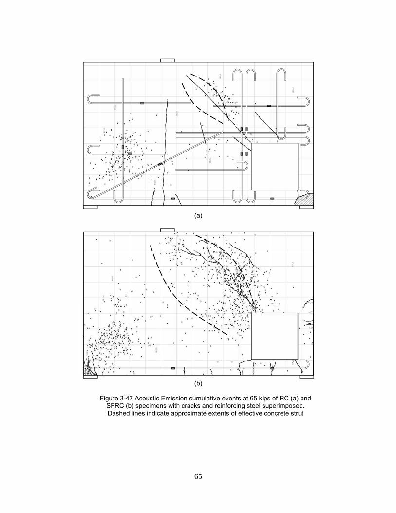
However, AE revealed that more energy was dissipated on the area between the

opening and the loading point of the SFRC specimen. Compared to RC, the SFRC specimen

showed many more hits in this area (see Figure 3-45). Extending the fiber bridging effect, it is

apparent that the concrete compressive strut is widened during loading. Where in the RC

specimen the compressive strut is effective only up to a certain width, the SFRC expands the

width of damage in the strut. Comparing the RC and the SFRC specimens in Figure 3-47, the

SFRC shows energy dissipated in a more wide area.

The inclusion of steel fibers in the concrete mix causes energy to be dispersed into

smaller, discrete amounts, which AE captures as hits. The RC specimen had the same amount

of energy dissipated, although in more concentrated amounts. Hence, the figure shows fewer

hits in the same region than the SFRC specimen. This agrees with crack observations that the

SFRC specimen had smaller, thinner cracks that branch out in random directions. The steel

fibers serve as a “bridge,” that enables forces to be redistributed from one area to the next. This

overcomes concrete’s weak tensile strength capacity and brittle nature.Also, the splitting

cracking along a compressive strut could be delayed due to the higher tensile strength of SFRC

compared to plain concrete.

59

(a)

(b)

Figure 3-41 Acoustic Emission cumulative events at 15 kips of RC (a) and

SFRC (b) specimens

60

(a)

(b)

Figure 3-42 Acoustic Emission cumulative events at 25 kips of RC (a) and

SFRC (b) specimens

61

(a)

(b)

Figure 3-43 Acoustic Emission cumulative events at 35 kips of RC (a) and

SFRC (b) specimens

62

(a)

(b)

Figure 3-44 Acoustic Emission cumulative events at 45 kips of RC (a) and

SFRC (b) specimens

63

(a)

(b)

Figure 3-45 Acoustic Emission cumulative events at 65 kips of RC (a) and

SFRC (b) specimens

64

(a)

(b)

Figure 3-46 Acoustic Emission cumulative events at 65 kips of RC (a) and

SFRC (b) specimens with cracks superimposed

65

(a)

(b)

Figure 3-47 Acoustic Emission cumulative events at 65 kips of RC (a) and

SFRC (b) specimens with cracks and reinforcing steel superimposed. Dashed lines indicate approximate extents of effective concrete strut

66

CHAPTER 4

COMPUTER AIDED STRUT-AND-TIE (CAST) ANALYSIS

4.1 Computer Aided Strut and Tie (CAST) Analysis – RC Specimen

The strut-and-tie model was analyzed using software developed by Tjhin and Kuchma

at the University of Illinois at Urbana-Champaign (2002). The materials properties obtained from

material tests were used for concrete and reinforcing steel in the models. By doing so, the

strength reduction factor φ was set to unity. Tie areas of 0.22 in2 and 0.44in2 was set for two

and four, No.3 reinforcing bars, respectively. The supports where modeled as a vertical reaction

on the left support and a vertical and horizontal reaction on the right support

The input procedure, are presented in Appendix A. The output files are presented in

Appendix B. The design load was 31.4 kips. The software’s capacity prediction feature was

used to estimate the capacity using the provided steel reinforcement, concrete struts and nodal

zones.

Additionally, the software has a feature that allows analysis of the nodes to ensure that

geometry and stress limits are not exceeded. The estimated capacity according to the software

was 41.2 kips for the RC specimen using the nominal material strengths (see Figure 4-2).

However, since the material strengths were determined by testing, the expected ultimate

capacity estimated by the software was 70.3 kips (see Figure 4-3). According to CAST, the

failure would occur by yielding of the diagonal tie. This is desirable in STM because it allows the

member to fail in a ductile manner as the reinforcing bars yield first before failure, as opposed to

brittle failure of the concrete struts.

67

Figure 4-1 Geometry and strut-and-tie model. Solid lines indicate tension tie and dashed lines indicate compressive strut. Units in in. and (mm)

The numbers in parenthesis (O/S) show the actual load divided the demand capacity.

For any value greater than one, the actual force is greater than the model allows; therefore, it

has failed. Depending on the analysis (predicted strength based on the model or design

strength) the program gives the tie that has analytically failed.

CAST precludes analysis if the truss system is not stable. Therefore, a support was

added to the right side of bottle-shaped strut from the loading point to the right support (see

Figure 4-2). This support is only required for the program to run the design and does not

calculate a reaction or calculates a very small reaction. The location was not critical, since other

joints that cause stability are also possible. Note that in Figure 4-2 that there are no over

strength elements. Therefore, all O/S ratios are less than one.

68

Figure 4-2 Strut and tie model analysis based on CAST at design load (numbers indicate the ratio between demand and capacity of each member; O/S indicated over strength)

Figure 4-3 Strut and tie model analysis based on CAST at ultimate load (unitless numbers indicate the ratio between demand to capacity of each member; O/S indicated over strength)

69

4.2 Computer Aided Strut and Tie (CAST) Analysis –RC Specimen with Single Bottom Tie

The same software discussed in the preceding sections was used to predict the

ultimate load the specimen would take if only the bottom steel reinforcing tie was used and

concrete tensile ties were assumed. The intent was to determine how much capacity the

specimen would gain by the inclusion of steel fibers, if any. The concrete tensile strength was

calculated using ACI 318-08 equation 9-8 (ACI 318, 2008):

f’t = 7.5 cf ' (psi), where

f’t = concrete tensile strength (psi)

f’c = 28 day concrete compressive strength from the cylinder

test (psi)

Researchers have suggested concrete tensile strength of 4 cf ' (psi) in a transverse

“compression field” stress (Al-Nahlawi, Wight, 1992), although the concrete tensile strength

used here is more commonly used in practice. The CAST analysis predicted the specimen

would fail at ultimate load of 14.26 kips. The concrete tensile strength was substituted for the

steel tensile strength. However, since CAST does not allow two different strengths to be used

for the same STM component, an “equivalent” area of steel was used for the bottom steel

tension tie used in the actual specimen. Hence, the RC CAST model and the SFRC CAST

model were able to develop the same tensile force in the bottom tie.

70

Figure 4-4 CAST model of RC specimen considering concrete’s tensile strength (numbers indicate demand/capacity of each member; O/S indicated over strength)

Following the same procedure from the RC specimen, the bottom steel tie was also

extended into the left support, although the CAST model does not require this, provided

sufficient anchorage is provided.

From the model, one can see that the area on the top-right of the opening would be the

first to fail (see Figure 4-4 and Figure 4-5). The concrete tensile ties around this region have a

O/S ratio of 1.0, with ratios as previously described. The tie crossing perpendicular to the first

failed tie has the second highest force, with a O/S ratio or near one. Since the compressive

strength of the concrete was kept the same, the values for the compressive struts was very

low, as expected for a corresponding low specimen load. Obviously, the model with the

concrete tensile strength was not adequate for the first beam’s design load. This is due to plain

concrete’s very low tensile strength resisted in the ties of the model, although the compressive

strength of the concrete struts was very high.

71

Figure 4-5 CAST model of RC specimen considering concrete’s tensile strength with crack mapping overlay

72

CHAPTER 5

CONCLUSIONS AND RECOMMENDED FUTURE WORK

5.1 Summary and Conclusions

The performance of using steel fiber reinforced concrete was compared to a very

widely-used and accepted design method envisioned more than 100 years ago by Ritter and

Mörsch, which was further developed by Schlaich, et al. Although the strut-and-tie model is

gaining acceptance by the design professions, it is nonetheless cumbersome and at times,

ambiguous. Issues such as openings are not explicitly addressed in the ACI 318 Code. Less

experienced designers might overlook the importance of proper detailing, leading to unexpected

structural behavior due to poor detailing.

The concept of reinforcing brittle material with fibers is as old as the pyramids built by

the ancient Egyptians (Mehta and Monteiro, 2006). Reinforcing concrete with steel fibers has

been used to reduce material in structural slabs (ACI 544-96, 1996). Developments in the ability

to control the characteristics of plastic concrete has facilitated the use of concrete reinforced

with various types of fibers.

The performance of the SFRC specimen compared very well to the RC specimen

designed using the strut-and-tie model. Generally, the cracks of the SFRC were much smaller in

width than those of the RC specimen. The sudden energy release of the RC specimen was

mitigated in the SFRC specimen, due to fiber bridging effect, as seen visually and measured by

Acoustic Emission. Although there was no steel reinforcing in the area adjacent to the opening

in the SFRC specimen, the beam took nearly the same load as the heavily reinforced RC

specimen. The SFRC specimen failed as the fibers pulled off in the diagonal crack from the

opening to the loading point.

73

An analysis was performed using the same procedure as the RC specimen, except that

concrete’s tensile strength, as recommended by the literature, was used in place of tension ties

and one steel tie from support to support. The failure mode was in agreement with CAST’s

analysis that predicted failure near the opening leading to the loading point. The specimen’s

ultimate load increased by approximately four times as predicted by analysis, due to the

inclusion of steel fibers in the concrete matrix.

The concrete strain was more predictive for the SFRC specimen. Although the

measured strain was higher for the SFRC specimen than RC near the support with the opening,

the SFRC specimen did not have large pieces of concrete spalled. At about 58 kips, the

concrete’s strain in the left support became negative for the RC specimen. The STM model

would not have predicted a tensile stress on the support opposite the opening. In addition, strain

gage 14 measured a small compressive stress on the steel tensile tie.

The SFRC steel reinforcement tensile force increased more linearly than in the RC

specimen. At the SFRC’s ultimate load, the bottom tensile tie’s force was 2.81 kips. The same

bottom tensile tie’s force was 0.97 kips at the same load. However, the RC specimen saw a

tremendous strain increase slightly above this load, where as the SFRC specimen failed in

diagonal crack splitting.

The true load-deformation response was not presented due to experimental data loss

during testing. From the presented load-deformation response, however, it has been shown that

the SFRC specimen behaves similarly to the specimen designed with STM. Additionally, from

the observed failure of the SFRC specimen, the SFRC specimen failed in a controlled manner,

as the diagonal crack widened, with no brittle behavior. The result of this behavior can be

attributed to the steel fibers being pulled from the concrete matrix.

In summary, the complete replacement of conventional reinforcing bars by deformed

steel fibers at a volume of 1.5% is a feasible alternative to the current practice. Also, the SFRC

specimen had better damage control than the RC specimen in terms of limiting cracking under

service and ultimate loading. The SFRC specimen showed twice the ultimate capacity as used

74

in design, even with only bottom flexural reinforcement. It is expected that design deep beams

with openings can be significantly simplified by using the proposed material solution.

Acoustic emission proved to be an effective tool to identify crack development and

failure mechanism. In addition, acoustic emission identified to the increase in strength of the

SFRC specimen resulted from the wider compressive strut than that of conventional RC

specimen. The higher effective compressive strength of the strut (due to greater tensile strength

of SFRC) could be another factor that led to the higher ultimate strength of the SFRC specimen.

The following table summarizes analysis and testing performed on deep beam with

single opening:

Table 5.1 Summary of analysis and experimental testing

RC Specimen RC with only bottom reinforcement

SFRC with only bottom

reinforcement

Design Load (kips) 31.4 - 14.3

Expected Load

(kips)

70.25 14.3 -

Expected Load

(kips)

70* - 65

*Testing stopped due to instability

The RC specimen did take longer to construct since it had many reinforcing bars and

there was much time invested in making sure that the reinforcing bars were properly placed,

tied and had correct cover. On the other hand, constructing the SFRC specimen took very little

time, since it had only two reinforcing bars. In an actual full sized beam, this issued would be

aggravated because beams like these would be cast vertically and access to formwork would

be limited.

75

5.2 Recommended Future Work

After completing the research, it was found the following issues should be investigated:

1. Similar deep beams should be tested using additional shear reinforcement to

investigate stresses generated around web openings in beams.

2. Similar deep beams with different geometry and opening configuration should be

investigated.

3. The effect of varying SFRC fiber dosages should be investigated on deep beams with

web openings to evaluate its performance on structural applications.

4. The performance of different steel fibers should be investigated.

5. Further comparisons between conventional reinforced concrete and SFRC in structural

applications

6. Develop a design aid that enables practitioners to design using SFRC for structural

applications

76  

 

 

 

 

 

 

 

 

 

APPENDIX A

CAST INPUT DATA - RC

77  

The specimen’s geometry was generated according to the software’s instructions. The loading and boundary conditions were also established.

Figure A-1 General user-interface of CAST

The material properties as obtained from Chapter II were provided. Since there were the actual values,

phi values were set to unity, as previously discussed.

Figure A-2 General properties defined

78  

Concrete struts were defined according to ACI 318. The two types were bottle-shaped and prismatic

shaped concrete struts.

Figure A-3 Concrete Strut Types

Steel tensile ties were defined as either a single tie or a double tie. Since there was two No. 3 bars per

layer, a single tie consisted of 0.22 in2 and 0.44in2, respectively.

79  

Figure A-4 Steel tensile ties

Another aspect of STM that must be considered is the nodal region. Nodes were either compression on

all sides (C-C-C), tension on one side (C-C-T), or tension on more than one side (C-T-T). Accordingly, the

strength-reduction ratios as recommended by ACI were used.

80  

Figure A-5 Defining Node Types

The specimen was analyzed for adequacy for the given load. The software gives a color-coded graphical

representation of the stresses in the concrete struts, as well as numerical analysis of the nodal zones.

Any overstress component is coded in red and an over-strength (O/S) ratio greater than 1.

Figure A-6 Graphical interpretation of output data

81  

 

 

 

 

 

 

 

 

 

APPENDIX B

CAST OUTPUT FILE FOR RC SPECIMEN

82  

C A S T - Computer Aided Strut-and-Tie - Version 0.9.11 (Last Updated on 1/26/04)

File Name: Deep Beam1_w-ACI bottle Strut.txt

Date and Time Created: 9/27/2008 4:00:31 PM

Associated Input Data File Name: Deep Beam1_w-ACI bottle Strut.CST

P R O J E C T D E S C R I P T I O N:

PROJECT NAME: Deep Beam w/ Opening

DESIGNER: CAF

DATE: 7/28/2008

PROJECT NOTE: Original by Brena

D E S I G N C A L C U L A T I O N R E S U L T S:

LOAD CONDITION: LC1

ELEMENTS: ELEMNENT ID Force Stress Stress Limit/Yield Force

(k) (psi) (psi) (k) E1 10.99 24968 - 44

E10 11.4 25905 - 44

E11 4.13 18777 - 22

E12 4.69 21325 - 22

83  

E13 4.32 19636 - 22

E14 4.31 19569 - 22

E15 -9.75 738 3943 -

E16 -9.34 707 3943 -

E18 5.7 12952 - 44

E19 9.8 44557 - 22

E2 10.99 24968 - 44

E20 -8.21 1493 5257 -

E21 -5.92 1076 5257 -

E22 -7.91 1198 3943 -

E23 5.7 25905 - 22

E24 11.4 25905 - 44

E25 5.92 13444 - 44

E26 -10.51 1593 5257 -

E3 6.68 15183 - 44

E30 -1.16 88 5257 -

E31 -7.17 1086 3943 -

E40 -6.37 724 5257 -

E41 -11.23 1276 3943 -

E44 -31.3 2371 5257 -

E5 -5.98 679 3943 -

E6 -4.32 655 5257 -

E7 -4.13 469 5257 -

E81 -15.31 1391 5257 -

E84 -14.22 1293 5257 -

E85 -14.07 1279 5257 -

E86 5.34 24265 - 22

E88 -15.03 1366 5257 -

E89 -15.19 1381 5257 -

E9 6.71 15242 - 44

E90 5.14 23383 - 22

E91 -15.02 1365 5257 -

E92 -20.07 2281 5257 -

ELEMENT ID STRESS RATIO f'c RATIO Beta RATIO

E1 0.25 NA NA E10 0.259 NA NA E11 0.188 NA NA

84  

E12 0.213 NA NA E13 0.196 NA NA E14 0.196 NA NA E15 0.187 0.119 0.14 E16 0.179 0.114 0.135 E18 0.13 NA NA E19 0.446 NA NA E2 0.25 NA NA E20 0.284 0.241 0.284 E21 0.205 0.174 0.205 E22 0.304 0.194 0.228 E23 0.259 NA NA E24 0.259 NA NA E25 0.134 NA NA E26 0.303 0.258 0.303 E3 0.152 NA NA E30 0.017 0.014 0.017 E31 0.276 0.176 0.207 E40 0.138 0.117 0.138 E41 0.324 0.206 0.243 E44 0.451 0.383 0.451 E5 0.172 0.11 0.129 E6 0.125 0.106 0.125 E7 0.089 0.076 0.089 E81 0.265 0.225 0.265 E84 0.246 0.209 0.246 E85 0.243 0.207 0.243 E86 0.243 NA NA E88 0.26 0.221 0.26 E89 0.263 0.223 0.263 E9 0.152 NA NA E90 0.234 NA NA E91 0.26 0.221 0.26

E92 0.434 0.369 0.434

NODES:

NODE ID NODE FACE FORCE STRESS STRESS LIMIT

(k) (psi) (psi)

85  

N1 E1 10.99 1665 3154 E19 9.8 1536 3154 E21 -5.92 1076 3154 E22 -7.91 1198 3154 E30 -1.16 88 3154 E31 -7.17 1086 3154

N10 E18 5.7 863 3154 E20 -8.21 1493 3154 E25 5.92 896 3154

N11 E18 5.7 863 4206 E19 9.8 1536 4206 E88 -15.03 1366 4206 E89 -15.19 1381 4206 E92 -20.07 2281 4206

N12 E20 -8.21 1493 4206 E21 -5.92 1076 4206 E23 5.7 863 4206

N13 E22 -7.91 1198 3154 E23 5.7 863 3154 E24 11.4 1727 3154 E25 5.92 896 3154

N14 E26 -10.51 1593 5257 E31 -7.17 1086 5257 E44 -31.3 2371 5257 E81 -15.31 1391 5257 E91 -15.02 1365 5257

N2 E1 10.99 1665 3154 E2 10.99 1665 3154 E10 11.4 1727 3154 E24 11.4 1727 3154

N24 E41 -11.23 1276 5257 N27 E44 -31.3 2371 5257 N3 E2 10.99 1665 3154 E3 6.68 1012 3154 E12 4.69 1422 3154 E40 -6.37 724 3154

N35 E81 -15.31 1391 3154 E84 -14.22 1293 3154 E90 5.14 585 3154

86  

N38 E85 -14.07 1279 3154 E90 5.14 585 3154 E91 -15.02 1365 3154

N4 E3 6.68 1012 4206 E7 -4.13 469 4206 E15 -9.75 738 4206 E41 -11.23 1276 4206

N44 E85 -14.07 1279 3154 E86 5.34 607 3154 E88 -15.03 1366 3154

N45 E84 -14.22 1293 3154 E86 5.34 607 3154 E89 -15.19 1381 3154

N46 E92 -20.07 2281 NA N5 E6 -4.32 655 4206 E9 6.71 1016 4206 E16 -9.34 707 4206 E26 -10.51 1593 4206 E30 -1.16 88 4206

N6 E5 -5.98 679 4206 E7 -4.13 469 4206 E13 4.32 1309 4206

N7 E5 -5.98 679 4206 E6 -4.32 655 4206 E11 4.13 1252 4206

N8 E9 6.71 1016 3154 E10 11.4 1727 3154 E14 4.31 1305 3154 E40 -6.37 724 3154

N9 E11 4.13 1252 3154 E12 4.69 1422 3154 E13 4.32 1309 3154 E14 4.31 1305 3154 E15 -9.75 738 3154

E16 -9.34 707 3154

NODE ID NODE FACE STRESS RATIO f'c RATIO Beta RATIO

N1 E11 0.397 0.202 0.238 E12 0.451 0.23 0.27

87  

E13 0.415 0.212 0.249 E14 0.414 0.211 0.248 E15 0.234 0.119 0.14 E16 0.224 0.114 0.135

N10 E11 0.397 0.202 0.238 E12 0.451 0.23 0.27 E13 0.415 0.212 0.249 E14 0.414 0.211 0.248 E15 0.234 0.119 0.14 E16 0.224 0.114 0.135

N11 E11 0.397 0.202 0.238 E12 0.451 0.23 0.27 E13 0.415 0.212 0.249 E14 0.414 0.211 0.248 E15 0.234 0.119 0.14 E16 0.224 0.114 0.135

N12 E11 0.397 0.202 0.238 E12 0.451 0.23 0.27 E13 0.415 0.212 0.249 E14 0.414 0.211 0.248 E15 0.234 0.119 0.14 E16 0.224 0.114 0.135

N13 E11 0.397 0.202 0.238 E12 0.451 0.23 0.27 E13 0.415 0.212 0.249 E14 0.414 0.211 0.248 E15 0.234 0.119 0.14 E16 0.224 0.114 0.135

N14 E11 0.397 0.202 0.238 E12 0.451 0.23 0.27 E13 0.415 0.212 0.249 E14 0.414 0.211 0.248 E15 0.234 0.119 0.14 E16 0.224 0.114 0.135

N2 E11 0.397 0.202 0.238 E12 0.451 0.23 0.27 E13 0.415 0.212 0.249 E14 0.414 0.211 0.248 E15 0.234 0.119 0.14

88  

E16 0.224 0.114 0.135 N24 E11 0.397 0.202 0.238

E12 0.451 0.23 0.27 E13 0.415 0.212 0.249 E14 0.414 0.211 0.248 E15 0.234 0.119 0.14 E16 0.224 0.114 0.135

N27 E11 0.397 0.202 0.238 E12 0.451 0.23 0.27 E13 0.415 0.212 0.249 E14 0.414 0.211 0.248 E15 0.234 0.119 0.14 E16 0.224 0.114 0.135

N3 E11 0.397 0.202 0.238 E12 0.451 0.23 0.27 E13 0.415 0.212 0.249 E14 0.414 0.211 0.248 E15 0.234 0.119 0.14 E16 0.224 0.114 0.135

N35 E11 0.397 0.202 0.238 E12 0.451 0.23 0.27 E13 0.415 0.212 0.249 E14 0.414 0.211 0.248 E15 0.234 0.119 0.14 E16 0.224 0.114 0.135

N38 E11 0.397 0.202 0.238 E12 0.451 0.23 0.27 E13 0.415 0.212 0.249 E14 0.414 0.211 0.248 E15 0.234 0.119 0.14 E16 0.224 0.114 0.135

N4 E11 0.397 0.202 0.238 E12 0.451 0.23 0.27 E13 0.415 0.212 0.249 E14 0.414 0.211 0.248 E15 0.234 0.119 0.14 E16 0.224 0.114 0.135

N44 E11 0.397 0.202 0.238 E12 0.451 0.23 0.27

89  

E13 0.415 0.212 0.249 E14 0.414 0.211 0.248 E15 0.234 0.119 0.14 E16 0.224 0.114 0.135

N45 E11 0.397 0.202 0.238 E12 0.451 0.23 0.27 E13 0.415 0.212 0.249 E14 0.414 0.211 0.248 E15 0.234 0.119 0.14 E16 0.224 0.114 0.135

N46 E11 0.397 0.202 0.238 E12 0.451 0.23 0.27 E13 0.415 0.212 0.249 E14 0.414 0.211 0.248 E15 0.234 0.119 0.14 E16 0.224 0.114 0.135

N5 E11 0.397 0.202 0.238 E12 0.451 0.23 0.27 E13 0.415 0.212 0.249 E14 0.414 0.211 0.248 E15 0.234 0.119 0.14 E16 0.224 0.114 0.135

N6 E11 0.397 0.202 0.238 E12 0.451 0.23 0.27 E13 0.415 0.212 0.249 E14 0.414 0.211 0.248 E15 0.234 0.119 0.14 E16 0.224 0.114 0.135

N7 E11 0.397 0.202 0.238 E12 0.451 0.23 0.27 E13 0.415 0.212 0.249 E14 0.414 0.211 0.248 E15 0.234 0.119 0.14 E16 0.224 0.114 0.135

N8 E11 0.397 0.202 0.238 E12 0.451 0.23 0.27 E13 0.415 0.212 0.249 E14 0.414 0.211 0.248 E15 0.234 0.119 0.14

90  

E16 0.224 0.114 0.135 N9 E11 0.397 0.202 0.238 E12 0.451 0.23 0.27 E13 0.415 0.212 0.249 E14 0.414 0.211 0.248 E15 0.234 0.119 0.14

E16 0.224 0.114 0.135

91  

APPENDIX C

CAST OUTPUT FILE FOR RC SPECIMEN WITH SINGLE BOTTOM TIE 

 

 

 

 

 

 

 

 

 

 

 

 

92  

C. CAST OUTPUT FILE FOR RC SPECIMEN WITH SINGLE BOTTOM TIE

C A S T - Computer Aided Strut-and-Tie - Version 0.9.11 (Last Updated on 1/26/04)

File Name: Deep Beam_SFRC.txt

Date and Time Created: 9/27/2008 4:02:18 PM

Associated Input Data File Name: Deep Beam_SFRC.CST

P R O J E C T D E S C R I P T I O N:

PROJECT NAME: Deep Beam w/ Opening SFRC

DESIGNER: CAF

DATE: 7/28/2008

PROJECT NOTE: Original by Brena

D E S I G N C A L C U L A T I O N R E S U L T S:

LOAD CONDITION: LC1

93  

ELEMENTS: ELEMENT ID FORCE STRESS LIMIT/YIELD FORCE

(k) (psi) (psi) (k) E1 10.99 1248 - 5.19 E10 11.4 1295 - 5.19 E11 4.13 469 - 5.19 E12 4.69 533 - 5.19 E13 4.32 491 - 5.19 E14 4.31 489 - 5.19 E15 -9.75 738 3943 - E16 -9.34 707 3943 - E18 5.7 57 - 59.26 E19 9.8 1114 - 5.19 E2 10.99 1248 - 5.19 E20 -8.21 1493 5257 - E21 -5.92 1076 5257 - E22 -7.91 1198 3943 - E23 5.7 648 - 5.19 E24 11.4 1295 - 5.19 E25 5.92 672 - 5.19 E26 -10.51 1593 5257 - E3 6.68 759 - 5.19 E30 -1.16 88 5257 - E31 -7.17 1086 3943 - E40 -6.37 724 5257 - E41 -11.23 1276 3943 - E44 -31.3 2371 5257 - E5 -5.98 679 3943 - E6 -4.32 655 5257 - E7 -4.13 469 5257 - E81 -15.31 1391 5257 - E84 -14.22 1616 5257 - E85 -14.07 1599 5257 - E86 5.34 607 - 5.19 E88 -15.03 1366 5257 - E89 -15.19 1381 5257 - E9 6.71 762 - 5.19 E90 5.14 585 - 5.19 E91 -15.02 1365 5257 -

94  

E92 -20.07 1825 5257 -

ELEMENT ID STRESS RATIO f'c RATIO Beta RATIO

E1 2.116 NA NA E10 2.195 NA NA E11 0.796 NA NA E12 0.904 NA NA E13 0.832 NA NA E14 0.829 NA NA E15 0.187 0.119 0.14 E16 0.179 0.114 0.135 E18 0.096 NA NA E19 1.888 NA NA E2 2.116 NA NA E20 0.284 0.241 0.284 E21 0.205 0.174 0.205 E22 0.304 0.194 0.228 E23 1.098 NA NA E24 2.195 NA NA E25 1.139 NA NA E26 0.303 0.258 0.303 E3 1.287 NA NA E30 0.017 0.014 0.017 E31 0.276 0.176 0.207 E40 0.138 0.117 0.138 E41 0.324 0.206 0.243 E44 0.451 0.383 0.451 E5 0.172 0.11 0.129 E6 0.125 0.106 0.125 E7 0.089 0.076 0.089 E81 0.265 0.225 0.265 E84 0.307 0.261 0.307 E85 0.304 0.258 0.304 E86 1.028 NA NA E88 0.26 0.221 0.26 E89 0.263 0.223 0.263

95  

E9 1.292 NA NA E90 0.991 NA NA E91 0.26 0.221 0.26

E92 0.347 0.295 0.347

NODES:

NODE ID NODE FACE FORCE STRESS STRESS

LIMIT

(k) (psi) (psi)

N1 E1 10.99 1665 3154 E19 9.8 1536 3154 E21 -5.92 1076 3154 E22 -7.91 1198 3154 E30 -1.16 88 3154 E31 -7.17 1086 3154

N10 E18 5.7 863 3154 E20 -8.21 1493 3154 E25 5.92 896 3154

N11 E18 5.7 863 4206 E19 9.8 1536 4206 E88 -15.03 1366 4206 E89 -15.19 1381 4206 E92 -20.07 1825 4206

N12 E20 -8.21 1493 4206 E21 -5.92 1076 4206 E23 5.7 863 4206

N13 E22 -7.91 1198 3154 E23 5.7 863 3154 E24 11.4 1727 3154 E25 5.92 896 3154

N14 E26 10.51 1593 5257 E31 -7.17 1086 5257 E44 -31.3 2371 5257 E81 -15.31 1391 5257 E91 -15.02 1365 5257

96  

N2 E1 10.99 1665 3154 E2 10.99 1665 3154 E10 11.4 1727 3154 E24 11.4 1727 3154

N24 E41 -11.23 1276 5257 N27 E44 -31.3 2371 5257 N3 E2 10.99 1665 3154 E3 6.68 1012 3154 E12 4.69 1422 3154 E40 -6.37 724 3154

N35 E81 -15.31 1391 3154 E84 -14.22 1616 3154 E90 5.14 585 3154

N38 E85 -14.07 1599 3154 E90 5.14 585 3154 E91 -15.02 1365 3154

N4 E3 6.68 1012 4206 E7 -4.13 469 4206 E15 -9.75 738 4206 E41 -11.23 1276 4206

N44 E85 -14.07 1599 3154 E86 5.34 607 3154 E88 -15.03 1366 3154

N45 E84 -14.22 1616 3154 E86 5.34 607 3154 E89 -15.19 1381 3154

N46 E92 -20.07 1825 NA N5 E6 -4.32 655 4206 E9 6.71 1016 4206 E16 -9.34 707 4206 E26 -10.51 1593 4206 E30 -1.16 88 4206

N6 E5 -5.98 679 4206 E7 -4.13 469 4206 E13 4.32 1309 4206

N7 E5 -5.98 679 4206 E6 -4.32 655 4206 E11 4.13 1252 4206

N8 E9 6.71 1016 3154

97  

E10 11.4 1727 3154 E14 4.31 1305 3154 E40 -6.37 724 3154

N9 E11 4.13 1252 3154 E12 4.69 1422 3154 E13 4.32 1309 3154 E14 4.31 1305 3154 E15 -9.75 738 3154

E16 -9.34 707 3154

NODE ID NODE FACE STRESS RATIO f'c RATIO Beta RATIO

N1 E11 0.397 0.202 0.238 E12 0.451 0.23 0.27 E13 0.415 0.212 0.249 E14 0.414 0.211 0.248 E15 0.234 0.119 0.14 E16 0.224 0.114 0.135

N10 E11 0.397 0.22 0.238 E12 0.451 0.23 0.27 E13 0.415 0.212 0.249 E14 0.414 0.211 0.248 E15 0.234 0.119 0.14 E16 0.224 0.114 0.135

N11 E11 0.397 0.22 0.238 E12 0.451 0.23 0.27 E13 0.415 0.212 0.249 E14 0.414 0.211 0.248 E15 0.234 0.119 0.14 E16 0.224 0.114 0.135

N12 E11 0.397 0.22 0.238 E12 0.451 0.23 0.27 E13 0.415 0.212 0.249 E14 0.414 0.211 0.248 E15 0.234 0.119 0.14 E16 0.224 0.114 0.135

N13 E11 0.397 0.22 0.238 E12 0.451 0.23 0.27 E13 0.415 0.212 0.249

98  

E14 0.414 0.211 0.248 E15 0.234 0.119 0.14 E16 0.224 0.114 0.135

N14 E11 0.397 0.22 0.238 E12 0.451 0.23 0.27 E13 0.415 0.212 0.249 E14 0.414 0.211 0.248 E15 0.234 0.119 0.14 E16 0.224 0.114 0.135

N2 E11 0.397 0.22 0.238 E12 0.451 0.23 0.27 E13 0.415 0.212 0.249 E14 0.414 0.211 0.248 E15 0.234 0.119 0.14 E16 0.224 0.114 0.135

N24 E11 0.397 0.22 0.238 E12 0.451 0.23 0.27 E13 0.415 0.212 0.249 E14 0.414 0.211 0.248 E15 0.234 0.119 0.14 E16 0.224 0.114 0.135

N27 E11 0.397 0.22 0.238 E12 0.451 0.23 0.27 E13 0.415 0.212 0.249 E14 0.414 0.211 0.248 E15 0.234 0.119 0.14 E16 0.224 0.114 0.135

N3 E11 0.397 0.202 0.238 E12 0.451 0.23 0.27 E13 0.415 0.212 0.249 E14 0.414 0.211 0.248 E15 0.234 0.119 0.14 E16 0.224 0.114 0.135

N35 E11 0.397 0.22 0.238 E12 0.451 0.23 0.27 E13 0.415 0.212 0.249 E14 0.414 0.211 0.248 E15 0.234 0.119 0.14 E16 0.224 0.114 0.135

99  

N38 E11 0.397 0.22 0.238 E12 0.451 0.23 0.27 E13 0.415 0.212 0.249 E14 0.414 0.211 0.248 E15 0.234 0.119 0.14 E16 0.224 0.114 0.135

N4 E11 0.397 0.22 0.238 E12 0.451 0.23 0.27 E13 0.415 0.212 0.249 E14 0.414 0.211 0.248 E15 0.234 0.119 0.14 E16 0.224 0.114 0.135

N44 E11 0.397 0.22 0.238 E12 0.451 0.23 0.27 E13 0.415 0.212 0.249 E14 0.414 0.211 0.248 E15 0.234 0.119 0.14 E16 0.224 0.114 0.135

N45 E11 0.397 0.22 0.238 E12 0.451 0.23 0.27 E13 0.415 0.212 0.249 E14 0.414 0.211 0.248 E15 0.234 0.119 0.14 E16 0.224 0.114 0.135

N46 E11 0.397 0.22 0.238 E12 0.451 0.23 0.27 E13 0.415 0.212 0.249 E14 0.414 0.211 0.248 E15 0.234 0.119 0.14 E16 0.224 0.114 0.135

N5 E11 0.397 0.202 0.238 E12 0.451 0.23 0.27 E13 0.415 0.212 0.249 E14 0.414 0.211 0.248 E15 0.234 0.119 0.14 E16 0.224 0.114 0.135

N6 E11 0.397 0.202 0.238 E12 0.451 0.23 0.27 E13 0.415 0.212 0.249

100  

E14 0.414 0.211 0.248 E15 0.234 0.119 0.14 E16 0.224 0.114 0.135

N7 E11 0.397 0.22 0.238 E12 0.451 0.23 0.27 E13 0.415 0.212 0.249 E14 0.414 0.211 0.248 E15 0.234 0.119 0.14 E16 0.224 0.114 0.135

N8 E11 0.397 0.202 0.238 E12 0.451 0.23 0.27 E13 0.415 0.212 0.249 E14 0.414 0.211 0.248 E15 0.234 0.119 0.14 E16 0.224 0.114 0.135

N9 E11 0.397 0.202 0.238 E12 0.451 0.23 0.27 E13 0.415 0.212 0.249 E14 0.414 0.211 0.248 E15 0.234 0.119 0.14

E16 0.224 0.114 0.135

 

101

REFERENCES

AASHTO, “AASHTO LRFD Bridge Design Specifications,” American Association of State

Highway and Transportation Officials, first edition, Washington, DC, 1994, 1091 pp.,

including interim revisions for 1996 and 1997.

ACI Committee 318. (2008), “Building Code Requirements for Structural Concrete (ACI 318-08)

and Commentary (318R-08),” American Concrete Institute, Farmington Hills, MI

ACI Committee 544. (1996), “Report on Fiber Reinforced Concrete (ACI 544.1 R-96),” American

Concrete Institute, Farmington Hills, MI

ASTM A 370 – 07a, “Standard Test Methods and Definitions for Mechanical Testing of Steel

Products,” ASTM International, West Conshohocken, PA, pp. 191-195.

ASTM A 615/A 615M – 07, “Standard Specification for Deformed and Plain Carbon-Steel Bars

for Concrete Reinforcement,” ASTM International, West Conshohocken, PA, pp. 325-

329.

ASTM C 1609/C 1609M - 06, “Standard Test Method for Flexural Performance of Fiber-

Reinforced Concrete (Using Beam With Third-Point Loading),” ASTM International,

West Conshohocken, PA, pp. 831-838.

ASTM C 39/C 39M – 05, “Standard Test Method for Compressive Strength Cylindrical Concrete

Specimens,” ASTM International, West Conshohocken, PA, pp. 22-28

ASTM C 78 – 02, “Test Method for Flexural Strength of Concrete (Using Simple Beam with

Third-Point Loading,” ASTM International, West Conshohocken, PA, pp. 40-42.

ASTM C 617 – 98 (2003), “Practice for Capping Cylindrical Concrete Specimens,” ASTM

International, West Conshohocken, PA, pp. 324-328.

Al-Nahlawi, Khaled A., Wight, James K., 1992, “Beam Analysis Using Concrete Tensile

Strength in Truss Models,” ACI Structural Journal, V. 89, No. 3, May-Jun., pp.284-289.

102

Ashour, A. F.; Chung, H. S.; and Yang, K. H., 2007, “Influence of Inclined Web Reinforcement

on Reinforced Concrete Deep Beams with Openings,” ACI Structural Journal, V. 104,

Sept-Oct., pp. 580-589.

Breña, S. F.; and Morrison, M. C., 2007, “Factors Affecting Strength of Elements Designed

Using Strut-and-Tie Models,” ACI Structual Journal, V. 104, No. 3, May-June., pp. 267-

277.

Bae, S.; Breen, J. E,; Ley, M. T.; Ridding, K. A.,; and Widianto., 2007, “Experimental Verification

of Strut-and-Tie Model Design Method,” ACI Structural Journal, V. 104, No. 6, Nov-

Dec., pp. 749-755.

Breen, J. E,; and Maxwell, B. S., 2000, “Experimental Evaluation of Strut-and-Tie Model Applied

to Deep Beam with Opening,” ACI Structural Journal, V. 97, No. 1, Jan-Feb., pp. 142-

149.

Casanova, P.; and Rossi, P., “High Strength Concrete Beams Submitted to Shear: Steel Fibers

Versus Stirrups,” Ed. Banthia, N.; MacDonald, C.; and Tatnall, P., “Structural

Applications of Fiber Reinforced Concrete,” American Concrete Institute, Farmington

Hills, MI., 1999.

Chao, S.-H. (2008), "Achieving “Green” Concrete through the Use of High Performance Fiber

Reinforced Concrete," ASCE Texas Section Fall Meeting, Addison, TX, October 3rd,

2008.

Chen, B. S.; Hagenbergerm, M. J.; and Breen, J. E., 2002, “Evaluation of Strut-and-Tie

Modeling Applied to Dapped Beams with Opening,” ACI Structural Journal, V. 99, No. 4,

July-Aug., pp. 445-450

Colombo, S., Main, I.G., Forde, M.C., 2003, ASCE Journal of Materials in Civil Engineering,

V.15, No. 3, Jun., pp. 280-286.

CSA Committee A23.3, “Design of Concrete Structures (CAN3-A23.3-M84),” Canadian

Standards Association, Rexdale, ON, Canada, 1984, pp. 281

103

Darwish, I. Y. S.; and Narayanan, R., 1988, “Fiber Concrete Deep Beams in Shear,” ACI

Structural Journal, V. 85, No.2, Mar-April, pp. 141-149.

Dupont, D.; and Vandewalle, L., “Shear Capacity of Concrete Beams Containing Longitudinal

Reinforcement and Steel Fibers.” Ed. Banthia, N.; Criswell, M.; Tatnall, P.; and Folliard,

K., Innovations in Fiber-Reinforced Concrete for Value, American Concrete Institute,

Farmington Hills, MI., 2003.

Hibbeler, R.C., 2005, “Mechanics of Materials,” 6th Edition, Prentice Hall p.123.

Kuchma, D.; and Park, J. W., 2007, “Strut-and-Tie Model Analysis for Strength Prediction of

Deep Beams,” ACI Structural Journal, V. 104, No. 6, Nov-Dec, pp. 657-666.

Kuchma, Daniel; Yindeesuk, Sukit; Nagle, Thomas; Hart, Jason; Lee, Heui H.,

2008,“Experimental Validation of Strut-and-Tie Method for complex Regions,” ACI

Structural Journal, V. 105, No. 5, Sep-Oct., pp. 578-589.

Mehta, P. Kumar, Monteiro, Paulo J.M., 2006, “Concrete – Microstructure, Properties, and

Materials,” 3rd Edition, McGraw-Hill, New York, p. 502.

Mörsch, E., Concrete-Steel Construction, E.P. Goodrich, translation, McGraw-Hill, New York,

1909, pp. 368

Narayanan, R., and Darwish, I. Y. S., 1988, “Fiber Concrete Deep Beams in Shear,” ACI

Structural Journal, 85, No. 2, March-April., 141-149.

Ritter, W., “Die Bauweise Hennebique,” Schweizerische Bauzeitung, V. 33, No. 7, Feb. 1899,

pp. 59-61.

Schlaich, J.; Schäfer, K.; and Jennewein, M., 1987, “Toward a Consistent Design of Structural

Concrete,” PCI Journal, Special Report, V. 32, No. 3, pp. 74-150.

Tan, K. H.; and Zhang, N., 2007, “Size effect in RC deep beams: Experimental investigation and

STM verification,” Engineering Structures, V. 29, pp. 3241- 3254.

United States Green Building Council, News and Events: In the News: Recession or Not, Green

Building to Keep Growing, LyndaDePillis, New York Observer, November 13, 2008.

http://www.usgbc.org/News/USGBCInTheNewsDetails.aspx?ID=3876

104

BIOGRAPHICAL INFORMATION

Carlos Flores was born in Zacapuato, Gro., Mexico on May 7, 1983, the son of Virgilio and

Carolina Flores. After completing his work at Adamson High School, Dallas, Texas, in 2001, he entered

Mountain View College in Dallas, Texas. He received his Associates Degree in Arts in 2003. He soon

entered The University of Texas at Arlington. He received the degree of Bachelor of Science in

Architecture in May 2006. In August of 2007 he entered the Graduate School at the University of Texas at

Arlington. During the following year he was employed by Wiss, Janney, Elstner, Associates and

Raymond L. Goodson, Jr., Consulting Engineers. He is currently employed by Nelson Consulting

Engineers focusing on investigation, rehabilitation and retrofit of new and existing structures. Carlos lives

in Dallas, Texas. His short-term plans are to marry Esbeide Pereznegron, earn design experience and

become a registered design professional. He will consider pursuing a doctoral degree as his long-term

career goal. Carlos enjoys spending time with his family, various construction-related activities and

spending his time in church. He regularly volunteers with non-for-profit organizations such as The

Hispanic Scholarship Fund, Habitat for Humanity, ACE high school mentor program, among others, giving

back to his community.