Embed Size (px)
Citation preview
Un
de
r a
xia
l te
nsi
le l
oa
din
g
Pe
rfo
rm
an
ce
of
Mic
ro
pil
es
Lisanne Meerdink
MSc Thesis - Report
June 2013

2 PERFORMANCE OF MICROPILES UNDER AXIAL TENSILE LOADING |MSc Thesis
CHAPTER 1| PREFACE 3
Performance of Micropiles Under axial tensile loading
Master Thesis
Date: 25 June 2013
Student: Lisanne Meerdink
TU Delft
Master student Geo-engineering
Exam committee: Prof. ir. A.F. van Tol
Chairman
TU Delft, CiTG, section Geo-engineering
Ir. H.J. Lengkeek
Witteveen + Bos
Ing. H.J. Everts
TU Delft, CiTG, section Geo-engineering
Dr.ir. C. van der Veen
TU Delft, CiTG, section Structural engineering

4 PERFORMANCE OF MICROPILES UNDER AXIAL TENSILE LOADING |MSc Thesis
CHAPTER 1| PREFACE 5
PREFACE
In this master thesis a study to the performance and modelling of micropiles is made. The
research is performed at the TU Delft, faculty of Civil Engineering and Geosciences at the
department of Geo-engineering and at Witteveen + Bos Deventer within the group of
Geotechnical and Hydraulic Engineering.
In May 2012 I started exploring the topic of micropiles. Now I present a method to
calculate the axial spring stiffness of micropiles. During the working in this thesis I did not
only learn about micropiles from literature and discussions, but I have also been to two
project to see micropiles being constructed, tested and excavated. I would like to thank
Witteveen + Bos for this opportunity, I enjoyed this practical experience.
I would like to thank Arny Lengkeek for his never ending enthusiasm, support and helpful
input. Further I would like to thank Cor van der Veen, Frits van Tol and Bert Everts for
their suggestions and recommendations. I have learned a lot from all the discussions and
remarks.
Others I would like to thank are my friends, family and colleagues at Witteveen + Bos. The
discussing about the topic or just listening to my complains helped me through the study.
Finally I would like to thank my boyfriend Frank for his support and my parents for their
support and advise throughout the years of studying.
Lisanne Meerdink
Delft, 25 June 2013

6 PERFORMANCE OF MICROPILES UNDER AXIAL TENSILE LOADING |MSc Thesis
CHAPTER 1| SUMMARY 7
SUMMARY
This thesis focuses on the modelling of the pile head displacement of micropiles when
loaded under tension. Although nowadays pile tests are performed to measure the
capacity and axial spring stiffness of micropiles, the focus was always to check the
maximum bearing capacity. Different methods have been developed for predicting the
maximum shear stress: cone penetration tests in combination with empirical parameters
or using effective stresses. In the Netherlands there has not been much research
performed in the determination of the pile head displacement. The traditional calculation
method assumes a rigid pile for the development of the shear stresses and is therefore
conservative when used for micropile design. In countries like France (FOREVER [1]) and
the USA (API [2]) the determination of the pile head displacement is performed using load-
transfer functions along the pile shaft.
The model developed in this thesis is based on displacement calculation of the French
research project on micropiles “FOREVER” [1] and the traditional Dutch method to
determine the shear stresses and maximum bearing capacity. It is therefore called the
Revised FOREVER model (RFM). The calculation of the maximum shaft friction and bearing
capacity is performed following the NEN 9997-1 [11]. To obtain the pile head displacement
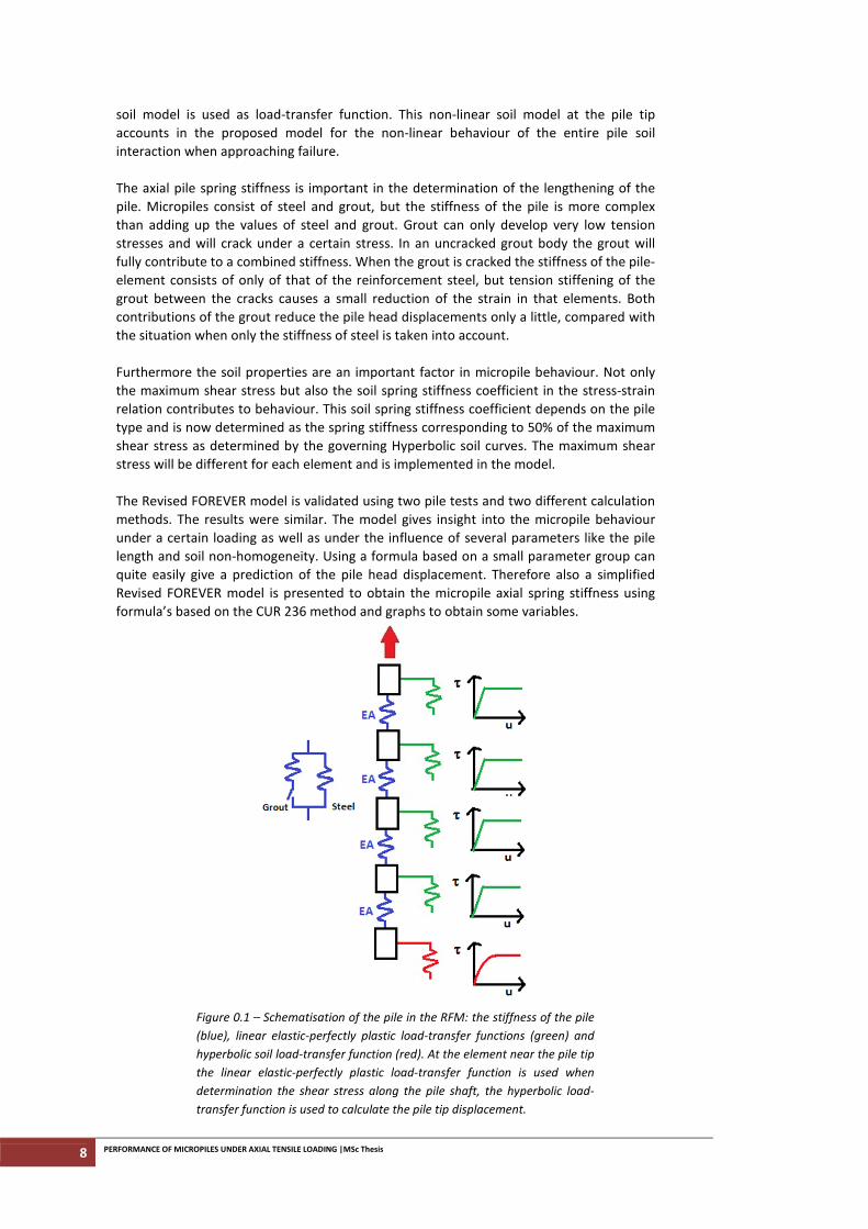
corresponding to a certain load, the pile is discretised in elements in series. A
schematisation of the model is given in Figure 0.1. All elements are assumed to be
connected by springs representing the axial stiffness of the pile. In addition each element
is connected with a spring that represents the soil. The behaviour of these soil springs is
determined by load-transfer functions. Although the soil behaves non-linear, a linear
elastic-perfectly plastic load-transfer function is assumed for the soil behaviour along the
pile shaft. Due to this linearity and the stiffness between the pile elements, the shear
stress along the pile shaft as a function of depth can be solved analytically. When
calculating the pile displacement, a more realistic non-linear load-transfer function will be
used for the calculation of the pile tip displacement.
Under a small load the micropile-soil interface will behave elastic: with increasing
displacements the shear stress in the interface will increase. This shear stress has a
maximum, given by the soil properties and the pile-soil bond. Under a certain tensile load
the upper part of the pile-soil interface will reach this maximum shear stress; this interface
behaves plastic. With increasing load the transition point between the plastic and the
elastic interface continues to the pile tip until the maximum bearing capacity of the pile
has developed. The displacement of the elements and the total lengthening of the pile
follow from Hooke’s law and the local equilibrium. The axial force in the pile will decrease
with increasing depth due to the load transfer through the shaft-soil interface. This axial
force in an element causes lengthening of the element (local strain) and by summation of
the small lengthening of each element the total lengthening of the pile is calculated. The
pile tip has a displacement as well, as a result from the shear stress acting on the lowest
element near the pile tip. To determine this tip displacement a the non-linear Hyperbolic
8 PERFORMANCE OF MICROPILES UNDER AXIAL TENSILE LOADING |MSc Thesis
soil model is used as load-transfer function. This non-linear soil model at the pile tip
accounts in the proposed model for the non-linear behaviour of the entire pile soil
interaction when approaching failure.
The axial pile spring stiffness is important in the determination of the lengthening of the
pile. Micropiles consist of steel and grout, but the stiffness of the pile is more complex
than adding up the values of steel and grout. Grout can only develop very low tension
stresses and will crack under a certain stress. In an uncracked grout body the grout will
fully contribute to a combined stiffness. When the grout is cracked the stiffness of the pile-
element consists of only of that of the reinforcement steel, but tension stiffening of the
grout between the cracks causes a small reduction of the strain in that elements. Both
contributions of the grout reduce the pile head displacements only a little, compared with
the situation when only the stiffness of steel is taken into account.
Furthermore the soil properties are an important factor in micropile behaviour. Not only
the maximum shear stress but also the soil spring stiffness coefficient in the stress-strain
relation contributes to behaviour. This soil spring stiffness coefficient depends on the pile
type and is now determined as the spring stiffness corresponding to 50% of the maximum
shear stress as determined by the governing Hyperbolic soil curves. The maximum shear
stress will be different for each element and is implemented in the model.
The Revised FOREVER model is validated using two pile tests and two different calculation
methods. The results were similar. The model gives insight into the micropile behaviour
under a certain loading as well as under the influence of several parameters like the pile
length and soil non-homogeneity. Using a formula based on a small parameter group can
quite easily give a prediction of the pile head displacement. Therefore also a simplified
Revised FOREVER model is presented to obtain the micropile axial spring stiffness using
formula’s based on the CUR 236 method and graphs to obtain some variables.
Figure 0.1 – Schematisation of the pile in the RFM: the stiffness of the pile
(blue), linear elastic-perfectly plastic load-transfer functions (green) and
hyperbolic soil load-transfer function (red). At the element near the pile tip
the linear elastic-perfectly plastic load-transfer function is used when
determination the shear stress along the pile shaft, the hyperbolic load-
transfer function is used to calculate the pile tip displacement.
CHAPTER 1| LIST OF SYMBOLS 9
LIST OF SYMBOLS
a Rib height [mm]
a Constant [-]
A Area [mm2]
AR Area of the rib-projection [mm2]
b Constant [-]
c Rib spacing [mm]
cg Grout cover [mm]
Ctip Factor to determine the tip displacement [-]
Dg Diameter of the groutbody [mm]
Dp Diameter of the pile [mm]
Ds Diameter of the steel [mm]
Eg Young’s modulus of grout [kN/m2]
Es Young’s modulus of steel [kN/m2]
EA Stiffness of the pile [kN]
EcAc Combined stiffness grout and steel [kN]
f1 Factor for the effect of compaction [-]
f2 Factor for lowering the effective stress by the tension force [-]
f3 Lengthening factor [-]
fc Average of concrete strength of the test specimens [N/mm2]
fck Characteristic compressive cylinder strength [N/mm2]
fctk,0,05 Characteristic axial tensile strength of concrete 5% [N/mm2]
fctk,0905 Characteristic axial tensile strength of concrete 95 % [N/mm2]
fcm Mean value of axial tensile strength of concrete [N/mm2]
fcm,cube Cubic compressive strength [N/mm2]
fctm Mean value of axial tensile strength of concrete [N/mm2]
ft Rupture stress [N/mm2]
fyk Yield stress [N/mm2]
fR Relative rib factor [-]
lcr, ave Average crack distance [mm]
lcr, mac Maximum crack distance [mm]
ld Rib spacing [mm]
Lb Bond length of the micropile [m]
Lfree Free length of the micropile [m]
Ltot Total length of the micropile [m]
lm Transition length at fully developed crack phase [mm]
lst Transition length at not fully developed crack phase [mm]
Kpile Axial spring stiffness of the pile [kN/m]
kτ Soil spring stiffness [kN/m3]
kτ50 Soil spring stiffness coefficient, at 50% mobilisation of maximum
shear stress
[%/m]
N(z) Axial force in the pile on depth z [kN]
Ncr Normal force at which the grout starts to crack in the pile [kN]
10 PERFORMANCE OF MICROPILES UNDER AXIAL TENSILE LOADING |MSc Thesis
Ncr,g Normal force at which the grout starts to crack in the pile,
determined by only the grout
[kN]
P0
Micropile load [kN]
qc,z,exc Cone resistance at depth z [MPa]
rf Failure ratio [-]
Rt Maximum bearing capacity [MN]
Rt,d Design value of the bearing capacity [MN]
u0 Interface displacement at peak shear stress [mm]
u50 Interface displacement at 50% of the shear stress [mm]
ucreep Displacement due to creep of the soil [mm]
uhead Displacement of the pile head [mm]
uheave Displacement due to heave of the soil [mm]
ulength Displacement due to lengthening of the pile [mm]
Ur,c displacement steel bar relative to the concrete [mm]
utip Displacement of the pile tip [mm]
wmv ave Average crack width at fully developed crack phase [mm]
wmv max Maximum crack width at fully developed crack phase [mm]
wmo Mean crack width at not fully developed crack phase [mm]
z Depth [m]
zl Location of the transition point [m]
αe Ratio of E-moduli [-]
αt Shaft friction coefficient [-]
αts Tension stiffening factor [-]
β Variable factor (β=Leff/Lb) [-]
δ Interface friction angle at failure between pile and soil [degrees]
γ Bar geometry dependent constant [-]
γs,t Factor for safe design; material factor [-]
γm,var,qc Factor for safe design; variation in load [-]
ε
Strain [m/m]
εc1 Compressive strain in the concrete at the peak stress fc [‰]
εcu1 Ultimate compressive strain in the concrete [‰]
εg,cr Strain at which grout starts to crack [m/m]
Δεts Tension stiffening [m/m]
ε uk Strain at failure [m/m]
λ Effective reference length [m]
λ/Lb Scaling factor [-]
ρ Reinforcement ratio [-]
ρrep Density [kg/m3]
σs Stress in the steel at which cracking occurs [N/mm2]
σcr Concrete tensile strength at which cracking occurs [N/mm2]
σ'r Radial effective stresses on the shaft [N/mm2]
σ'rc Local equilibrium effective stress [N/mm2]
CHAPTER 1| LIST OF SYMBOLS 11
Δσ'r Change in the effective stress during loading [N/mm2]
Δσ’rp Change in the effective stress due to the principle stress rotation [N/mm2]
Δσ’rd Change in the effective stress due to th dilatation due to slip [N/mm2]
Δσ’rv Change in the effective stress due to the Poisson’s effect [N/mm2]
τ(z) Shear stress in the micropile-soil interface at depth z [kN/m2]
τb Bond between reinforcement and concrete [kN/m2]
τ Shaft shear stress [kN/m2]
τel Shear stress in the elastic phase of pile-soil interaction [kN/m2]
τi Shear stress in element i [kN/m2]
τmax Maximum shear stress [kN/m2]
τpl Shear stress in the plastic phase of pile-soil interaction [kN/m2]
τtip Shear stress in the tip-element [kN/m2]
ξm,n Correlation factor (relation to no. of tests) [-]

12 PERFORMANCE OF MICROPILES UNDER AXIAL TENSILE LOADING |MSc Thesis
CHAPTER 1| LIST OF SYMBOLS 13
CONTENTS
PREFACE ............................................................................................................................... 5
SUMMARY ............................................................................................................................. 7
LIST OF SYMBOLS ................................................................................................................. 9
1 INTRODUCTION .......................................................................................................... 15
1.1. Problem definition ............................................................................................ 15
1.2. Objectives .......................................................................................................... 16
1.3. Limitations......................................................................................................... 16
1.4. Lay-out of the report ......................................................................................... 16
2 MICROPILES ................................................................................................................ 17
2.1. Design of micropiles ......................................................................................... 18
2.2. Materials ............................................................................................................ 19
3 AXIALLY LOADED PILES ............................................................................................ 23
4 MODELLING AXIALLY LOADED MICROPILES IN TENSION .................................... 27
4.1. Load-transfer mechanism ................................................................................ 27
4.2. Schematisation of axially loaded micropiles ................................................... 28
4.3. Analytical Basic model ...................................................................................... 29
5 STRUCTURAL BEHAVIOUR ........................................................................................ 41
5.1. Young’s modulus of the materials .................................................................... 42
5.2. Bond steel-grout interface ................................................................................ 46
5.3. Vertical cracking ............................................................................................... 51
5.4. Horizontal cracking........................................................................................... 51
5.5. Combined stiffness ............................................................................................ 58
5.6. Conclusions ....................................................................................................... 64
6 SOIL BEHAVIOUR ....................................................................................................... 65
6.1. Shear stress and vertical loading direction ..................................................... 66
6.2. Softening and the lengthening effect ............................................................... 68
6.3. Load-transfer function ...................................................................................... 71
6.4. Soil spring stiffness ........................................................................................... 72
6.5. Non-homogeneous soil ..................................................................................... 73
6.6. Conclusions ....................................................................................................... 74
7 FINAL MODEL: RFM ................................................................................................... 75
7.1. Revised FOREVER model .................................................................................. 75
7.2. Validation of the model .................................................................................... 76
7.3. Micropile behaviour .......................................................................................... 79
14 PERFORMANCE OF MICROPILES UNDER AXIAL TENSILE LOADING |MSc Thesis
7.4. Influence of the parameters ............................................................................. 80
7.5. Simplified RFM .................................................................................................. 85
8 CONCLUSIONS AND RECOMMENDATIONS ............................................................. 89
8.1. Conclusions ....................................................................................................... 89
8.2. Recommendations ............................................................................................ 91
REFERENCES ...................................................................................................................... 93
APPENDICES ........................................................................................................... in a separate bundle
CHAPTER 1| INTRODUCTION 15
1 INTRODUCTION
Micropiles are long and slender piles used as foundation elements and are applied in
various situations. For example, they are used as tension piles in building pits, or as
compression piles for a foundation in soft soil. Micropiles cast in place and have a
diameter of maximum 300 mm. The piles consist of a grout column with a steel bar in the
centre. The design of micropiles is inspired by the ground anchor technique to support
horizontal forces in the soil. Micropiles are used worldwide and different anchorpile
systems are developed, such as the Ischebeck anchor in Germany and the GEWI-pile and
the Leeuwanker anchorpile in the Netherlands. Micropile technology is nowadays
commonly used worldwide, though in the Netherlands it is still a relatively new technique.
1.1. Problem definition The micropile technique is based on the ground anchor technique combined with regular
(concrete/steel/wooden) piles. Despite the knowledge about these systems and the
experience with micropile so far, the theory behind the performance of the vertical
micropile has not been very well developed. While the micropile and inclined anchors
have similarities, there are important differences in composition, function and knowledge
about the pile’s behaviour. Inclined ground anchors can bear tension loads, are relatively
short and have a short grout body (about 5 m) on the lower end of the anchor
reinforcement. On the other hand micropiles can have lengths that can be up to 30 meter
and they have a long groutbody. Compression as well as tension loads can be transferred
by micropiles.
The biggest difference is the gap in knowledge between the two anchoring systems. At
first, ground anchors are tested a lot so there is knowledge about their bearing capacity.
All ground anchors in a building pit are tested for capacity; it is an easy and relatively quick
test. The use of micropiles is relatively new as is their testing. The testing of micropiles on
location is much more difficult and costly, especially for micropiles in underwater
concrete. Secondly, ground anchors are always prestressed, so the axial performance
becomes less important and therefore not critical in the design. This axial performance
gives a relation between the pile head displacement which will occur due to the load on
top. Micropiles can be prestressed but this is difficult and expensive and it is therefore not
done. As a result it is important to know the axial pile performance to determine the
expected pile head displacement.
16 PERFORMANCE OF MICROPILES UNDER AXIAL TENSILE LOADING |MSc Thesis
So, while the bearing capacity of the micropile is sufficient (tested by some test piles and
test procedures on final-piles), it is still important to know the axial pile performance of
the pile. This is because of contract regulations: a pile is often made by a different
contractor than the structure above (for example underwater concrete floor). The axial
spring stiffness requirement of the piles is in the contract, so it has to be known. In
building pits different axial spring stiffnesses of the piles will not give a problem
immediately. However if there is a relatively big difference in axial performance between
compartments (for example piles and diaphragm wall), problems can occur in the
structure above (for example underwater concrete). Moreover, when micropiles are used
in foundation-repair, its axial performance must be in relation with the surrounding
foundations to keep the pile head displacements at about the same value.
1.2. Objectives Currently, there are some models available to determine the axial pile performance and
their (maximum) bearing capacity or (maximum) displacement of the pile head. These
formulas are based on theory and experience, but the real behaviour of the axially loaded
piles is not well understood. Will the grout stick to the pile, how is the development of the
shaft capacity? Most testing is done to obtain only the maximum bearing capacities. The
development of bearing capacity or, more important, the displacements are not clear.
The objective of this thesis is to investigate the performance of axially loaded micropiles
under tension and make a model to calculate the axial spring stiffness of micropiles. Main
topics are the development of the Young’s modulus of steel, the influence of crack
formations of the grout and the implementation of non-homogeneous soil. Additional
topics are the influence of load direction on the capacity and the existence of softening of
sand. A model that implements these factors will be made. Finally the influence of the
different parameters on the performance of the micropile is discussed.
A literature study on the development of shaft friction along the pile will be used to
develop a basic model. Research into the fields of grout-cracking, Young’s modulus of
steel, the development of shear stress and designing in non-homogeneous soils will be
implemented in this model to create the final model. Using the final model, the pile
performance and contribution of the different materials is discussed. In the end it is
discussed if the model can be simplified for practical use.
1.3. Limitations In this research only single micropiles loaded in tension are considered; only the shaft
friction creates bearing capacity and there is no group-influence. The focus will be on the
displacements due to soil-micropile interaction, and not on the determination of the
maximum capacity. The stiffness will be investigated, but only on the influence of the
behaviour of the pile itself: by mobilization of the shaft resistance and elasticity of the pile.
The heave and creep will be disregarded in the model. The model will be developed in
Excell using only a homogeneous layer of sand. As reinforcement different types of steel
will be considered.
1.4. Lay-out of the report In chapter 2 an introduction to micropiles is given. Chapter 3 describes the theory and
literature about axial micropile performance and the difference in methods to calculate
the pile displacement. This theory is used to model axially loaded piles in tension in
chapter 4. In chapter 5 the behaviour of the pile materials steel and grout are discussed
and in chapter 6 the (influence and) behaviour of the soil. The final model and its
possibilities are given in chapter 7. The report will end with conclusions and
recommendations in chapter 8.
CHAPTER 2| MICROPILES 17
2 MICROPILES
Micropiles, long and small piles, are often used for foundations in the Netherlands. These
piles are cast in place and can therefore be used in many situations. The original idea of
micropiles comes from Dr. Fernando Lizzi, an Italian civil engineer. In 1952 he started to
use the “pali radice” (root piles, micropiles) in networks to reconstruct buildings after
Wold War II. Nowadays micropiles are used for their high capacity and displacement
reduction as single piles. The design of this single pile type for foundations is based on
(inclined) ground anchors which for example are used to strengthen soil-resisting
sheetpiles. In the Netherlands, the use of these vertical variant of ground anchors started
about 15 years ago. A micropile is the combination of a drillhole diameter (as small as
possible), a high percentage of steel reinforcement as bearing element and an adequate
grouting technology which is able to transfer the load along the shaft.
The micropile can be used for different functions. Advantages of this system are that they
can bear high forces and can be adapted to the local circumstances due to its production
on location. Their regular use is as foundation element (tension pile) in building pits, in
combination with an underwater concrete floor as foundation for a new construction in
soft soil or when high forces are assumed such as in power pylons. They are also used
when there is a limited working height, in foundation retrofit or rehabilitation projects. In
these projects micropiles are not only useful for their high bearing capacity but also for the
minimum displacements that will occur and the minimum disturbance and vibration to
adjacent structures, soil and the environment.
In the definition of the code about the execution of mircorpiles [NEN-EN14199, 4],
micropiles are “piles which have a small diameter (smaller than 300 mm shaft diameter for
drilled piles and not greater than 150 mm shaft diameter or maximum shaft cross sectional
extension for driven piles)”. The US Federal Highway Administration has a more specified
definition formulated: “It is a small diameter, (less than 300 mm) drilled and grouted
replacement pile that is typically reinforced.” [1] So, these long, slender piles consist of
grout and reinforcement.
18 PERFORMANCE OF MICROPILES UNDER AXIAL TENSILE LOADING |MSc Thesis
Depending on the local soil conditions, piles can be made in lengths up to 30 meter and
can be used for tension and compression loads. Micropiles can be made in rock, sand and
soft soil. Their capacity depends on the soil and pile properties and can be more than
1000 kN as well in tension as in compression. Micropiles have their bearing capacity only
(tension) or mostly (compression) from the shaft friction. The end-bearing in compression
piles is relatively small due to the small cross section: this gives about 10-15% of the total
capacity [5].
2.1. Design of micropiles Micropiles are used in different countries and for various soil conditions. Over the years
many types of micropiles are therefore developed. Examples are the Ischebeck anchor in
Germany and the GEWI-pile and the Leeuwanker anchorpile in the Netherlands. Which
type of pile will be used depends on the soil properties in combination with the properties
of the pile. The bearing capacity of a pile depends on the soil layering, ground water,
grouting method and drilling method. The types are divided in groups by their execution
method, micropiles can be driven or drilled. Following the NEN14199, driving is the
method to bring the micropile into the ground to the required depth, such as hammering,
vibrating, pressing, screwing or by a combination of these or other methods. Drilling (or
boring) is the method of removing the soil or rock in an intermittent or continuous process.
The micropile classification used in the Netherlands is given in Table 2.1. Other countries
use the execution method as difference in micropile types as well, but the categories or
exact diameter can vary: The French define for driven as well as bored piles the maximum
diameter of 250 mm and classification is in Type I-IV [1]. In the USA they assume Type A-D:
Gravity filling (A), pressure grouting (B) and post grouting (C and D). This report will only
refer to a type of the Dutch classification.
While there are many different types, the overall idea of the construction of a micropile is
the generally the same. First a tube is drilled or driven (with or without casing) until the
required depth. In case of type C and D this tube is the final reinforcement, and the
grouting will be through pores in the reinforcement. For types A and B the tube is just a
tool, a massive steel bar will be placed in this tube as reinforcement. While pulling the
casing, grout is inserted under pressure in stages from tip to pile head. The quality of a
micropile is therefore different at each location and depends a lot on the drill manager’s
experience. Micropiles can be made with equipment from ground level, but the piles can
be made from a pontoon in the water as well. As micropiles are a kind of ground anchors,
they can be installed at any angle by using equipment similar to the material for ground
anchors. For more information about the execution of certain types is referred to the
CUR 236 [6].
Due to the sensitivity of the execution method for the quality, it is required to test a
minimum number of micropiles. Three types of tests are prescribed in CUR 236: a failure
test, suitability test and performance test. The failure test is done during the design phase
to obtain the suitability of the pile for the situation and the final design parameters (αt).
Some test piles made on the building site are loaded in phases until the displacements
(related to the time) are too large. The pile then ‘failed’ loading. This test must be done on
3 piles for each (geological) soil layer. The suitability test is done on 3 % of the working
piles, before the connection with the construction is made. The maximum load (Fp) in this
test equals the expected load of the construction on top, adapted to dynamic forces. This
load can be high, so the location of these tests has to be clear on forehand, to be sure the
reinforcement in the pile will not break. With the result of this test the bearing capacity
and axial stiffness of the piles can be checked. The performance test finally tests the axial
spring stiffness. A minimum of 3 % of the piles for use is tested up to load Fp.
CHAPTER 2| MICROPILES 19
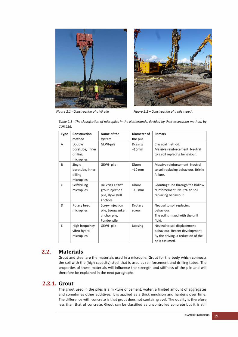
Figure 2.1 - Construction of a VF pile Figure 2.2 – Construction of a pile type A
Table 2.1 - The classifcation of micropiles in the Netherlands, devided by their excecution method, by
CUR 236.
Type Construction
method
Name of the
system
Diameter of
the pile
Remark
A Double
boretube, inner
drilling
micropiles
GEWI-pile Dcasing
+10mm
Classical method.
Massive reinforcement. Neutral
to a soil replacing behaviour.
B Single
boretube, inner
dilling
micropiles
GEWI- pile Dbore
+10 mm
Massive reinforcement. Neutral
to soil replacing behaviour. Brittle
failure.
C Selfdrilling
micropiles
De Vries Titan®
grout injection
pile, Dywi Drill
anchors
Dbore
+10 mm
Grouting tube through the hollow
reinforcement. Neutral to soil
replacing behaviour.
D Rotary head
micropiles
Screw injection
pile, Leeuwanker
anchor pile,
Fundex pile
Drotary
screw
Neutral to soil replacing
behaviour.
The soil is mixed with the drill
fluid.
E High frequency
vibro-hydro
micropiles
GEWI- pile Dcasing Neutral to soil displacement
behaviour. Recent development.
By the driving, a reduction of the
qc is assumed.
2.2. Materials Grout and steel are the materials used in a micropile. Grout for the body which connects
the soil with the (high capacity) steel that is used as reinforcement and drilling tubes. The
properties of these materials will influence the strength and stiffness of the pile and will
therefore be explained in the next paragraphs.
2.2.1. Grout The grout used in the piles is a mixture of cement, water, a limited amount of aggregates
and sometimes other additives. It is applied as a thick emulsion and hardens over time.
The difference with concrete is that grout does not contain gravel. The quality is therefore
less than that of concrete. Grout can be classified as uncontrolled concrete but it is still
20 PERFORMANCE OF MICROPILES UNDER AXIAL TENSILE LOADING |MSc Thesis
stronger as mortar. Cement type CEM II/B-M(S-V) 32.5 N is an example of used material.
This is Portland cement in which fly ash is added. The number 32,5 will indicate the
compression strength after 28 days, in this case >32,5 MPa but less than 52,5 MPa. The
indication ‘N’ explains the development of the strength over time: 0 MPa after 2 days,
>16,0 MPa after 7 days. The strengths given above are valid for construction in good
conditions (for example in laboratory).
It is assumed that grout has a quality comparable with B15. This is the maximum value
used for the design of a sandwich wand at the Central Station of Amsterdam-project [7]. A
second reference is made to the test on the TITAN tube, in fig. 5.12. In this laboratory test
the Young's modulus of grout is 23400 N/mm2. Because micropiles are cast-in-place this
strength and quality of the grout may be different. Especially for types C and D the grout is
expected to be mixed with soil, and this might influence the properties. A lower bound
estimate for the Young’s modulus of grout will be most appropriate. A Young's modulus of
20 000 MPa is therefore assumed. Other grout properties are given in Table 2.2.
Because the grout is in contact with the soil and groundwater, the cement must be
resistant for the local conditions, for example an aggressive environment. The groutbody
also contributes to corrosion protection of the reinforcement.
Table 2.2 – Properties of grout taken from B15 [8]
B15 = C12/15
Assumed secant modulus of elasticity of grout Ecm * 20 *103 [N/mm
2]
Characteristic compressive cylinder strength of concrete
at 28 days
fck 12 [N/mm2]
Characteristic compressive cubic strength of concrete f’ck; cube 15 [N/mm2]
Characteristic axial tensile strength of concrete 5% fctk,0,05 1,1 [N/mm2]
Characteristic axial tensile strength of concrete 95 % fctk,0905 2,0 [N/mm2]
Mean value of concrete cylinder compressive strength fcm 20 [N/mm2]
Mean value of axial tensile strength of concrete fctm 1,6 [N/mm2]
Compressive strain (=betonstuik) in the concrete at the
peak stress fc
εc1 1,8 [‰]
Ultimate compressive strain in the concrete εcu1 3,5 [‰]
Density ρrep 2400 [kg/m3]
* original Ecm of B15 is 27000 N/mm2
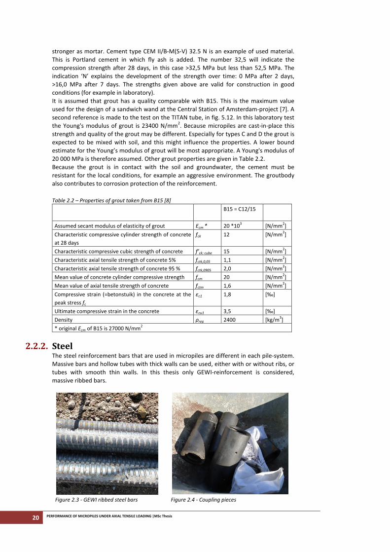
2.2.2. Steel The steel reinforcement bars that are used in micropiles are different in each pile-system.
Massive bars and hollow tubes with thick walls can be used, either with or without ribs, or
tubes with smooth thin walls. In this thesis only GEWI-reinforcement is considered,
massive ribbed bars.
Figure 2.3 - GEWI ribbed steel bars Figure 2.4 - Coupling pieces
CHAPTER 2| MICROPILES 21
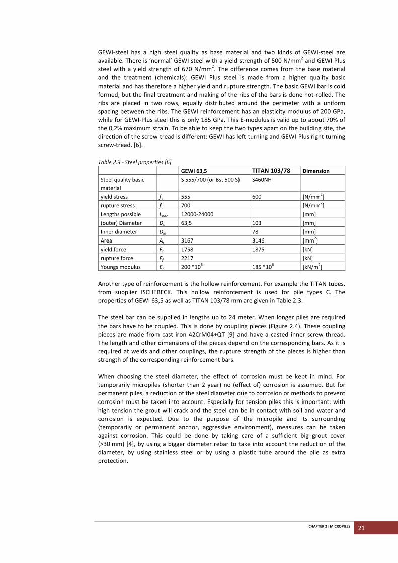
GEWI-steel has a high steel quality as base material and two kinds of GEWI-steel are
available. There is ‘normal’ GEWI steel with a yield strength of 500 N/mm2 and GEWI Plus
steel with a yield strength of 670 N/mm2. The difference comes from the base material
and the treatment (chemicals): GEWI Plus steel is made from a higher quality basic
material and has therefore a higher yield and rupture strength. The basic GEWI bar is cold
formed, but the final treatment and making of the ribs of the bars is done hot-rolled. The
ribs are placed in two rows, equally distributed around the perimeter with a uniform
spacing between the ribs. The GEWI reinforcement has an elasticity modulus of 200 GPa,
while for GEWI-Plus steel this is only 185 GPa. This E-modulus is valid up to about 70% of
the 0,2% maximum strain. To be able to keep the two types apart on the building site, the
direction of the screw-tread is different: GEWI has left-turning and GEWI-Plus right turning
screw-tread. [6].
Table 2.3 - Steel properties [6]
GEWI 63,5 TITAN 103/78 Dimension
Steel quality basic
material
S 555/700 (or Bst 500 S) S460NH
yield stress fy 555 600 [N/mm2]
rupture stress fu 700 [N/mm2]
Lengths possible Lbar 12000-24000 [mm]
(outer) Diameter Ds 63,5 103 [mm]
Inner diameter Din 78 [mm]
Area As 3167 3146 [mm2]
yield force Ft 1758 1875 [kN]
rupture force Ff 2217 [kN]
Youngs modulus Er 200 *106 185 *10
6 [kN/m
2]
Another type of reinforcement is the hollow reinforcement. For example the TITAN tubes,
from supplier ISCHEBECK. This hollow reinforcement is used for pile types C. The
properties of GEWI 63,5 as well as TITAN 103/78 mm are given in Table 2.3.
The steel bar can be supplied in lengths up to 24 meter. When longer piles are required
the bars have to be coupled. This is done by coupling pieces (Figure 2.4). These coupling
pieces are made from cast iron 42CrM04+QT [9] and have a casted inner screw-thread.
The length and other dimensions of the pieces depend on the corresponding bars. As it is
required at welds and other couplings, the rupture strength of the pieces is higher than
strength of the corresponding reinforcement bars.
When choosing the steel diameter, the effect of corrosion must be kept in mind. For
temporarily micropiles (shorter than 2 year) no (effect of) corrosion is assumed. But for
permanent piles, a reduction of the steel diameter due to corrosion or methods to prevent
corrosion must be taken into account. Especially for tension piles this is important: with
high tension the grout will crack and the steel can be in contact with soil and water and
corrosion is expected. Due to the purpose of the micropile and its surrounding
(temporarily or permanent anchor, aggressive environment), measures can be taken
against corrosion. This could be done by taking care of a sufficient big grout cover
(>30 mm) [4], by using a bigger diameter rebar to take into account the reduction of the
diameter, by using stainless steel or by using a plastic tube around the pile as extra
protection.

22 PERFORMANCE OF MICROPILES UNDER AXIAL TENSILE LOADING |MSc Thesis
CHAPTER 3| AXIALLY LOADED PILES 23
3 AXIALLY LOADED PILES
Micropile technology was developed by Dr. Lizzi in the early 1950’s. Since then a lot of
research is done into the design of this type of pile foundations. First this was focussed on
the maximum capacity. Nowadays the displacement of the pile head is more important
and is more intensively investigated. Different publications discuss the design and
execution methods of micropiles. For example, Eurocode 7 [10] gives the general rules
about geotechnical design, while NEN 9997 [11] is the Dutch implementation version of
this Eurocode. The rules for tension piles of CUR publication 2001-4 [3] are implemented
in this norm. Special rules for micropiles are the execution of micropiles in EN 14199 [4]
and the design and execution method in CUR publication 236 [6]. Other countries have
different norms and regulations. The German DIN 1054 [12] gives rules for ‘piles’ while the
ISO 19902 [13] and American API RP 2A-WSD [2] are offshore design norms. Different
authors and research projects have investigated the pile behaviour as well. Randolph
[14,15] focussed on the offshore piles but discussed the slenderness as an important
factor as well. This is useful in micropile design. In France the “Fondations Renforcées
Verticalement” [1] was a huge research project in the ‘90 to the performance of
micropiles. Research was done to single and network piles, static and cyclic loading. Many
more authors focussed on the calculation of the pile head displacement.
This chapter short discusses the axial pile performance of micropiles and the previous
research on this topic to calculate their load-displacement behaviour. The full literature
study is given in appendix A1.
Axial pile performance
The performance of a micropile is given by the load-displacement graph. This gives the
displacement of the pile head under a certain load. An example of a load-displacement
graph is given in Figure 3.1. It can be seen that from about 80% of the maximum load the
displacement increases fast with a small increase of load. This form of the load-
displacement graph is general for similar executed piles. Load-displacement graphs are
used in the design of foundations: when the load of a construction on top of a pile is
known, the displacement of the pile head can be derived. The relation between the two is
called the axial spring stiffness of the pile. The behaviour under the full loading process is
called the pile performance.
Different systems can be assumed to cause non-linear behaviour of the pile head stiffness.
At first, the development of the shear stress along the pile shaft is important in the design
of micropiles. With their long length, slender micropiles are assumed to be compressible.
The difference in displacements on pile top or head (closest to soil level) and pile tip
(deepest in the soil) can be substantial. While the soil-pile shear stress on the bottom of
the pile will start developing shear stresses, the top part can have exceeded this maximum
(possibility of softening). This effect can be seen in Figure 3.2. Secondly, the axial pile
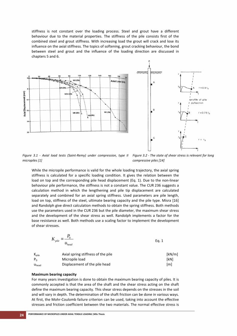
24 PERFORMANCE OF MICROPILES UNDER AXIAL TENSILE LOADING |MSc Thesis
stiffness is not constant over the loading process. Steel and grout have a different
behaviour due to the material properties. The stiffness of the pile consists first of the
combined steel and grout stiffness. With increasing load the grout will crack and lose its
influence on the axial stiffness. The topics of softening, grout cracking behaviour, the bond
between steel and grout and the influence of the loading direction are discussed in
chapters 5 and 6.
Figure 3.1 - Axial load tests (Saint-Remy) under compression, type II
micropiles [1]
Figure 3.2 - The state of shear stress is relevant for long
compressive piles [14]
While the micropile performance is valid for the whole loading trajectory, the axial spring
stiffness is calculated for a specific loading condition. It gives the relation between the
load on top and the corresponding pile head displacement (Eq. 1). Due to the non-linear
behaviour pile performance, the stiffness is not a constant value. The CUR 236 suggests a
calculation method in which the lengthening and pile tip displacement are calculated
separately and combined for an axial spring stiffness. Used parameters are pile length,
load on top, stiffness of the steel, ultimate bearing capacity and the pile type. Misra [16]
and Randolph give direct calculation methods to obtain the spring stiffness. Both methods
use the parameters used in the CUR 236 but the pile diameter, the maximum shear stress
and the development of the shear stress as well. Randolph implements a factor for the
base resistance as well. Both methods use a scaling factor to implement the development
of shear stresses.
0
pilehead
PK
u=
Eq. 1
Kpile Axial spring stiffness of the pile [kN/m]
P0
Micropile load [kN]
uhead Displacement of the pile head [m]
Maximum bearing capacity
For many years investigation is done to obtain the maximum bearing capacity of piles. It is
commonly accepted is that the area of the shaft and the shear stress acting on the shaft
define the maximum bearing capacity. This shear stress depends on the stresses in the soil
and will vary in depth. The determination of the shaft friction can be done in various ways.
At first, the Mohr-Coulomb failure criterion can be used, taking into account the effective
stresses and friction coefficient between the two materials. The normal effective stress is
CHAPTER 3| AXIALLY LOADED PILES 25
then taken as some ratio of the vertical effective stress. The appropriate ratio will depend
on the in-situ earth pressure coefficient, the method of installation of the pile and the
initial density of the sand. Values between 0,6 and 0,9 are used. The soil volumetric weight
over the depth, the interface friction angle and the pile type have to be known. The
ISO 19902 [13] and API [2] use a similar method: the undrained shear strength (for
cohesive soils, alfpha method) or the overburden pressure (for cohesionless soils, beta
method) are used. For the chosive soils a standart friction coefficeint will be taken as
relation between the overburden pressure and shear stress. This coefficient is based on
the relative density and soil classification. The Germain [DIN 1054, 12] have a general
method and use the soil classification only to use a empirical based shear stress. Another
method is to use cone penetration testing. This method is used in the Dutch design [3].
The measured cone resistances is combined with a shaft friction coefficient depending on
the pile type and measured in the field. The shear stress therefore follows from the cone
penetration strength, but it is reduced for different factors as excavation and tensile
loading. Using cone penetration tests is a simple, fast and economical method. Continues
records with depth are obtained so variations are taken into account. Compared with
laboratory testing undisturbed results are obtained.
Pile head displacement
The displacement of the micropile head is normally divided into two parts; the lengthening
of the pile and the displacement of the pile tip. In CUR 236 and DIN 1054 this lengthening
depends on the load on top and the maximum bearing capacity. These are quite simple
calculations and are because of the compressibility of micropiles too simple.
Displacements and shear stresses are related, and the shear stress has to be developed by
displacements before pile capacity is created. The lengthening therefore depends on the
developed shear stresses as well as the tip displacement. Several methods have been
developed to analyse in more detail the response of axially loaded piles. Closed form
solutions can be used, but these are for piles embedded in homogeneous linear elastic
half-space. Misra and FOREVER use this analytical method to determine lengthening of the
pile. For a Gibson soil, with increasing horizontal stress at greater depth, analytical
calculation methods are also possible [17].
To be able to implement the inhomogeneity of the soil as well as the more realistic non-
linear shear stress-strain behaviour of soil, numerical methods are used. Calculations can
be done by Finite Element Method [Yap, 18], Boundary Element Method and load-transfer
methods [Randolph and Wroth 19, Van Dalen 20]. In this thesis only load transfer
functions are considered. These functions can be used to determine the lengthening as
well as the pile tip displacement. Non-linear as well as linear elastic-perfectly plastic
functions can be used. The first implementations of the load-transfer method were based
on empirical data from instrumented piles. The API and FOREVER both use empirical based
load transfer functions along the pile shaft, based on the maximum shear stress and local
displacement that is needed to develop this maximum shear stress. Theoretical load-
transfer functions are now more used. Randolph and Worth [19] assumes that soil
deformations around a pile shaft can be idealized by concentric cylinders in shear. This
means that the displacement of the soil due to the pile axial load is mostly vertical and
radial displacements are negligible. This assumption corresponds with FEM analysis. The
stress-strain relation that Randolph and Worth assume is linear. Due to the use of soil
cylinders the shear stress depends on the local soil and pile parameters: displacement, soil
shear modulus, diameter of the pile and the area of influence. Mylonakis [21] uses this
method as well and defines a Winkler spring constant which represents the linear spring
behaviour of the soil using soil shear modulus. Other stress-strain relations as load transfer
functions are also possible: non-linear functions as the hyperbolic soil and modified
hyperbolic give a better representation of the soil behaviour.
26 PERFORMANCE OF MICROPILES UNDER AXIAL TENSILE LOADING |MSc Thesis
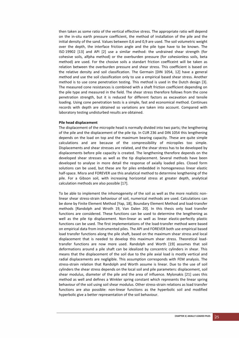
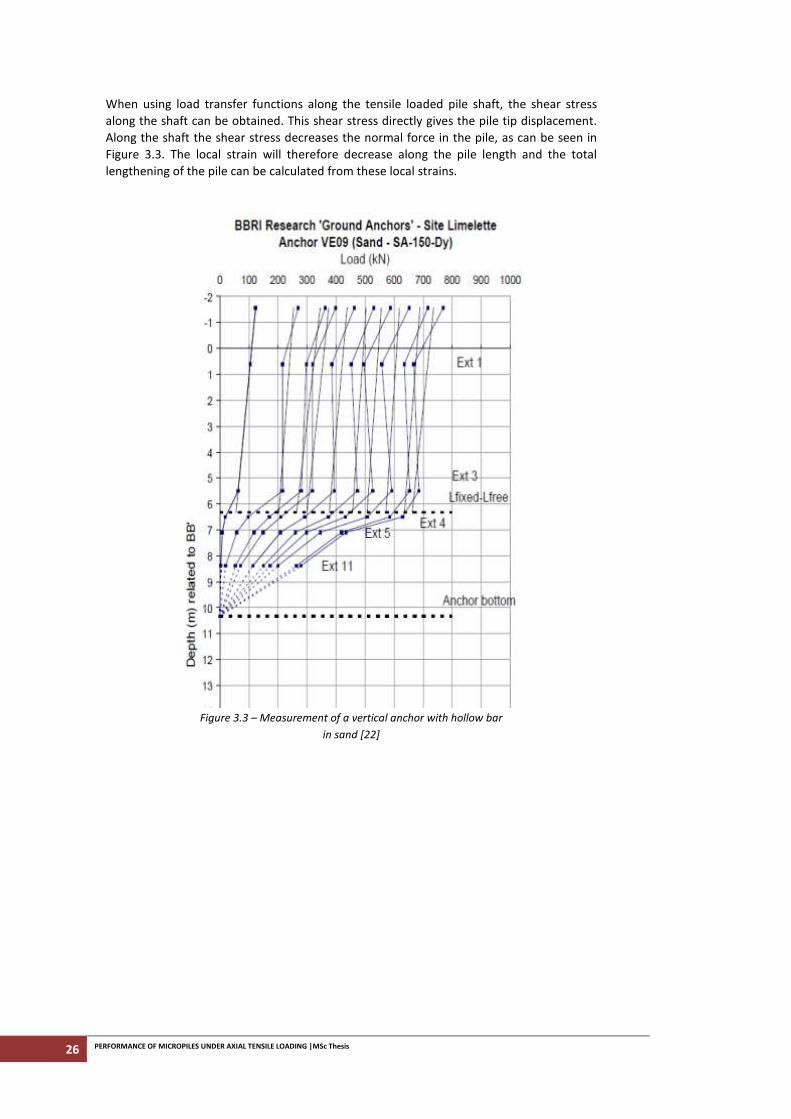
When using load transfer functions along the tensile loaded pile shaft, the shear stress
along the shaft can be obtained. This shear stress directly gives the pile tip displacement.
Along the shaft the shear stress decreases the normal force in the pile, as can be seen in
Figure 3.3. The local strain will therefore decrease along the pile length and the total
lengthening of the pile can be calculated from these local strains.
Figure 3.3 – Measurement of a vertical anchor with hollow bar
in sand [22]
CHAPTER 4| MODELLING AXIALLY LOADED MICROPILES IN TENSION 27
4 MODELLING AXIALLY
LOADED MICROPILES IN TENSION
In norms and regulations as the Eurocode 7, CUR 236 and API, calculation methods are
given for the determination of bearing capacity and displacements of micropiles. In the
Eurocode and CUR 236 a constant shear stress is assumed along the pile and therefore
over-estimating the displacement of the pile head. For rigid piles the shear stress along the
pile shaft is indeed constant. But micropiles are assumed to be flexible, resulting in a
different shear stress at pile head and pile tip and corresponding displacements. After all,
displacements are needed to create shear stress.
In this chapter the transfer of the load from the pile to the soil will be discussed and the
micropile-system is schematised to be able to model this load transfer. A first model to the
behaviour of micropiles will be made, focussing on the development of the pile head
displacement. Assumptions about load the load transfer are made in the first paragraph
and boundary conditions for the first model are discussed in section 4.3. To keep the
model simple and accessible the micropile soil interface is assumed to be linear elastic-
perfectly plastic and homogeneous with depth. Finally the modelled pile behaviour is
discussed and compared with the existing calculation method.
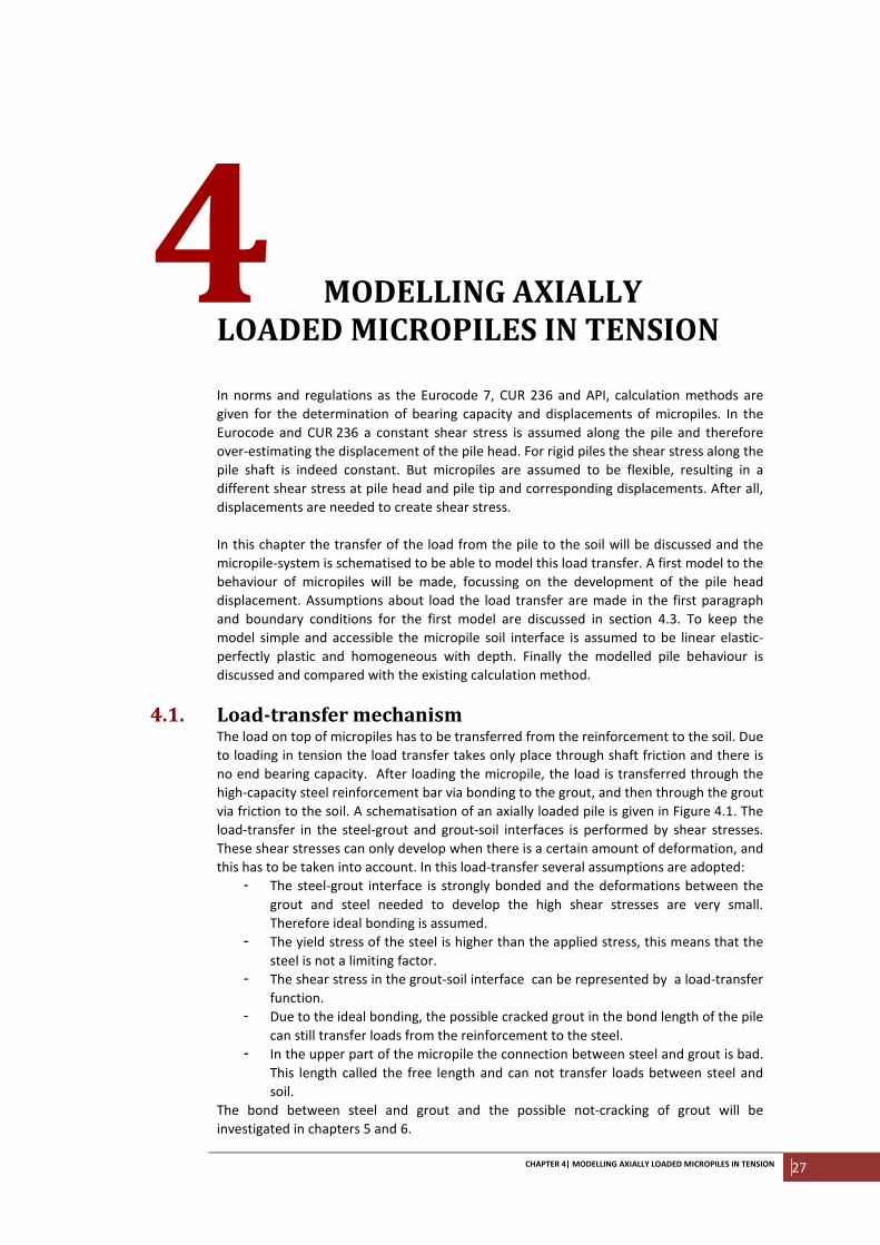
4.1. Load-transfer mechanism The load on top of micropiles has to be transferred from the reinforcement to the soil. Due
to loading in tension the load transfer takes only place through shaft friction and there is
no end bearing capacity. After loading the micropile, the load is transferred through the
high-capacity steel reinforcement bar via bonding to the grout, and then through the grout
via friction to the soil. A schematisation of an axially loaded pile is given in Figure 4.1. The
load-transfer in the steel-grout and grout-soil interfaces is performed by shear stresses.
These shear stresses can only develop when there is a certain amount of deformation, and
this has to be taken into account. In this load-transfer several assumptions are adopted:
- The steel-grout interface is strongly bonded and the deformations between the
grout and steel needed to develop the high shear stresses are very small.
Therefore ideal bonding is assumed.
- The yield stress of the steel is higher than the applied stress, this means that the
steel is not a limiting factor.
- The shear stress in the grout-soil interface can be represented by a load-transfer
function.
- Due to the ideal bonding, the possible cracked grout in the bond length of the pile
can still transfer loads from the reinforcement to the steel.
- In the upper part of the micropile the connection between steel and grout is bad.
This length called the free length and can not transfer loads between steel and
soil.
The bond between steel and grout and the possible not-cracking of grout will be
investigated in chapters 5 and 6.
28 PERFORMANCE OF MICROPILES UNDER AXIAL TENSILE LOADING |MSc Thesis
Figure 4.1 - Schematic of load-transfer mechanism Figure 4.2 - The state of shear stress is relevant
for long compressive piles. [14]
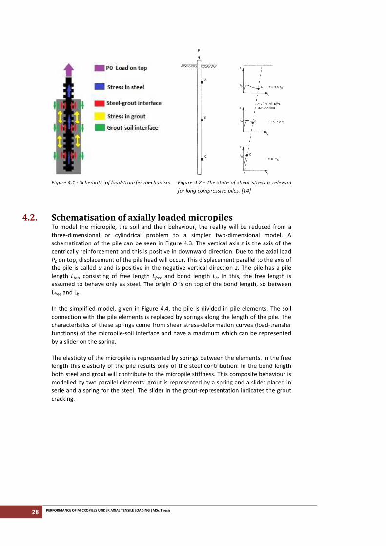
4.2. Schematisation of axially loaded micropiles To model the micropile, the soil and their behaviour, the reality will be reduced from a
three-dimensional or cylindrical problem to a simpler two-dimensional model. A
schematization of the pile can be seen in Figure 4.3. The vertical axis z is the axis of the
centrically reinforcement and this is positive in downward direction. Due to the axial load
P0 on top, displacement of the pile head will occur. This displacement parallel to the axis of
the pile is called u and is positive in the negative vertical direction z. The pile has a pile
length Ltot, consisting of free length Lfree and bond length Lb. In this, the free length is
assumed to behave only as steel. The origin O is on top of the bond length, so between
Lfree and Lb.
In the simplified model, given in Figure 4.4, the pile is divided in pile elements. The soil
connection with the pile elements is replaced by springs along the length of the pile. The
characteristics of these springs come from shear stress-deformation curves (load-transfer
functions) of the micropile-soil interface and have a maximum which can be represented
by a slider on the spring.
The elasticity of the micropile is represented by springs between the elements. In the free
length this elasticity of the pile results only of the steel contribution. In the bond length
both steel and grout will contribute to the micropile stiffness. This composite behaviour is
modelled by two parallel elements: grout is represented by a spring and a slider placed in
serie and a spring for the steel. The slider in the grout-representation indicates the grout
cracking.
CHAPTER 4| MODELLING AXIALLY LOADED MICROPILES IN TENSION 29
Figure 4.3 - Micropile, definitions Figure 4.4 - Schematization-model of a pile in the soil
4.3. Analytical Basic model In the development of the capacity and deformations of the pile factors like steel, grout,
soil and their interactions are variable and depend on the local circumstances. The
displacements follow from the shear stresses along the micropile. In this section the
different aspects that determine the performance of micropiles will be explained. First a
look is given to the maximum bearing capacity, followed by the development of the
capacity along the pile. In section 4.3.3 the displacement of the pile head is discussed.
Finally, the pile behaviour and differences with governing norm CUR 236 are discussed.
To keep the model simple, some assumptions are made:
- The soil is homogeneous.
- The soil shear stress-displacement (load-transfer function) is assumed to behave
linear elastic-perfectly plastic.
- Softening will not occur.
- In the bond length of the pile the grout is assumed to be fully cracked due to its
low tension capacity. Only the axial stiffness of steel is taken into account for the
displacement of the pile head.
- In the free length there is no load-transfer, only the axial stiffness is of steel is
taken into account.
To illustrate the calculation method a Basic pile is used. Its dimensions are given in Table
4.1. The specifications of the homogeneous soil are also given in this table. The total
bearing capacity of the 15 m pile is 1696 kN. The example calculations are done with
different loads, expressed in a % of the maximum capacity Rt.
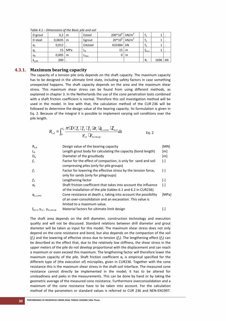
30 PERFORMANCE OF MICROPILES UNDER AXIAL TENSILE LOADING |MSc Thesis
Table 4.1 – Dimensions of the Basic pile and soil
D grout 0,2 m Esteel 200*106
kN/m2 f1 1 .
D steel 0,0635 m Egrout 20*106 kN/m
2 f2 1 .
αt 0,012 . EAsteel 633384 kN f3 1 .
qc 15 MPa Lb 15 m ξm,n 1 .
u0 0,005 m Lfree 0 m
kτ,50 200 . Rt 1696 kN
4.3.1. Maximum bearing capacity The capacity of a tension pile only depends on the shaft capacity. The maximum capacity
has to be designed in the ultimate limit state, including safety factors in case something
unexpected happens. The shaft capacity depends on the area and the maximum shear
stress. This maximum shear stress can be found from using different methods, as
explained in chapter 3. In the Netherlands the use of the cone penetration tests combined
with a shaft friction coefficient is normal. Therefore this soil investigation method will be
used in the model. In line with that, the calculation method of the CUR 236 will be
followed to determine the design value of the bearing capacity. Its formulation is given in
Eq. 2. Because of the integral it is possible to implement varying soil conditions over the
pile length.
1 2 3 ; ; ,
, 0; ;var;
bL t c z exc m n
t ds t m qc
D f f f qR dz
π α ξγ γ
⋅ ⋅ ⋅ ⋅ ⋅ ⋅ ⋅=
⋅∫
Eq. 2
Rt,d Design value of the bearing capacity [MN]
Lb Length grout body for calculating the capacity (bond length) [m]
Dg Diameter of the groutbody [m]
f1 Factor for the effect of compaction, is only for sand and soil
compressing piles (only for pile groups)
[-]
f2 Factor for lowering the effective stress by the tension force,
only for sands (only for pilegroups)
[-]
f3 Lengthening factor [-]
αt Shaft friction coefficient that takes into account the influence
of the installation of the pile (tables 6.1 and 6.2 in CUR236)
[-]
qc,,z,exc Cone resistance at depth z, taking into account the possibility
of an over-consolidation and an excavation. This value is
limited to a maximum value.
[MPa]
ξm,n, γs,t , γm,var,qc Material factors for ultimate limit design [-]
The shaft area depends on the drill diameter, construction technology and execution
quality and will not be discussed. Standard relations between drill diameter and grout
diameter will be taken as input for this model. The maximum shear stress does not only
depend on the cone resistance and bond, but also depends on the compaction of the soil
(f1) and the lowering of effective stress due to tension (f2). The lengthening effect (f3) can
be described as the effect that, due to the relatively low stiffness, the shear stress in the
upper meters of the pile do not develop proportional with the displacement and can reach
a maximum or even exceed this maximum. The lengthening factor will therefore lower the
maximum capacity of the pile. Shaft friction coefficient αt is empirical specified for the
different type of (the execution of) micropiles, given in CUR236. Together with the cone
resistance this is the maximum shear stress in the shaft-soil interface. The measured cone
resistance cannot directly be implemented in the model; it has to be altered for
unsteadiness and pieks in the measurements. This can be done by hand or by taking the
geometric average of the measured cone resistance. Furthermore overconsolidation and a
maximum of the cone resistance have to be taken into account. For the calculation
method of the parameters or standard values is referred to CUR 236 and NEN-EN1997.
CHAPTER 4| MODELLING AXIALLY LOADED MICROPILES IN TENSION 31
Also the factors ξm,n, γs,t and γm,var,qc on the measured soil-properties and material factors
for safe design can be found there.
4.3.2. Development of the shear stress along the pile Knowing the pile and soil properties, the development of the shear stress along the pile
under loading can be determined. In this case normal conditions are assumed in the
serviceability limit state. The maximum shear stress can follow from the bearing capacity,
but not directly: the lengthening effect will only lower the bearing capacity but not the
maximum shear stress. Only safety factor ξm,n for the influence of the number of cone
penetration tests (CPT’s) that is used, and not material parameters γs,t and γm,var,qc. In
short, the maximum shear stress can be formulated by:
max 1 2 , , ,t c z exc m nf f qτ α ξ= ⋅ ⋅ ⋅ ⋅ F1 Eq. 3
τmax Maximum shear stress in the micropile-soil interface [kN/m2]
To create shear stresses in the grout-soil interface a certain deformation is needed.
Different soil models can be used for this relation. To keep the model simple the behaviour
of the micropile-soil shaft interface is assumed to behave linear elastic-perfectly plastic.
This method of analysing the micropile’s performance is taken from FOREVER [1] and
Misra [16]. In appendix A2 their used formulas and the full mathematics are presented.
FOREVER takes the axial force in the pile as starting point, while Misra uses the shear
stress. When formulas are taken from FOREVER or Misra, this is referred by an F or M.
Using the following principles the shear stresses and displacements along the pile can be
determined:
• Local equilibrium of the micropile
( ) ( )gdN z D z dzπ τ= ⋅ F1
Eq. 4
N(z) Axial force in the pile on depth z [kN]
τ(z) Shear stress in the micropile-soil interface at depth z [kN/m2]
• Linear elasticity of the pile
( )( )
N zz
EAε =
F2b Eq. 5
ε
Strain [m/m]
EA Stiffness of the pile [kN]
• Theory of shaft friction interface mobilization
0
max 0
( ) for u u
( ) for u u
z k u
zττ
τ τ= ≤
= ≥
F3 Eq. 6
F3 Eq. 7
u0 Interface displacement at peak shear stress [m]
kτ Soil spring stiffness [kN/m3]
And boundary conditions:
• At pile head z=0, the normal force is the load on top N=P0
• At pile tip z=Lb, the normal force N=0
32 PERFORMANCE OF MICROPILES UNDER AXIAL TENSILE LOADING |MSc Thesis
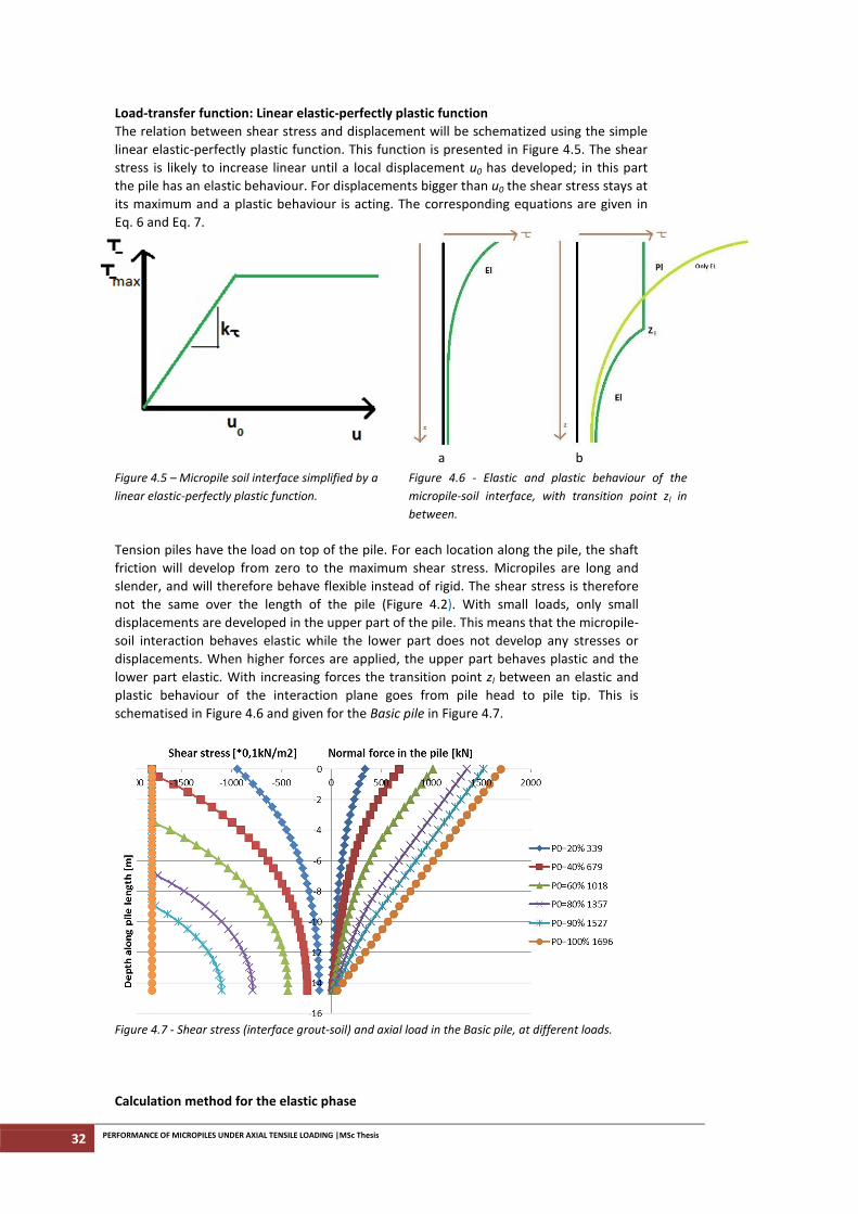
Load-transfer function: Linear elastic-perfectly plastic function
The relation between shear stress and displacement will be schematized using the simple
linear elastic-perfectly plastic function. This function is presented in Figure 4.5. The shear
stress is likely to increase linear until a local displacement u0 has developed; in this part
the pile has an elastic behaviour. For displacements bigger than u0 the shear stress stays at
its maximum and a plastic behaviour is acting. The corresponding equations are given in
Eq. 6 and Eq. 7.
a b
Figure 4.5 – Micropile soil interface simplified by a
linear elastic-perfectly plastic function.
Figure 4.6 - Elastic and plastic behaviour of the
micropile-soil interface, with transition point zl in
between.
Tension piles have the load on top of the pile. For each location along the pile, the shaft
friction will develop from zero to the maximum shear stress. Micropiles are long and
slender, and will therefore behave flexible instead of rigid. The shear stress is therefore
not the same over the length of the pile (Figure 4.2). With small loads, only small
displacements are developed in the upper part of the pile. This means that the micropile-
soil interaction behaves elastic while the lower part does not develop any stresses or
displacements. When higher forces are applied, the upper part behaves plastic and the
lower part elastic. With increasing forces the transition point zl between an elastic and
plastic behaviour of the interaction plane goes from pile head to pile tip. This is
schematised in Figure 4.6 and given for the Basic pile in Figure 4.7.
Figure 4.7 - Shear stress (interface grout-soil) and axial load in the Basic pile, at different loads.
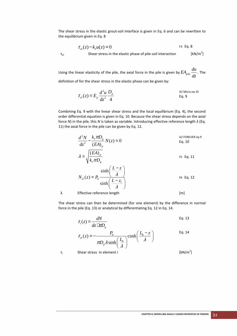
Calculation method for the elastic phase
CHAPTER 4| MODELLING AXIALLY LOADED MICROPILES IN TENSION 33
The shear stress in the elastic grout-soil interface is given in Eq. 6 and can be rewritten to
the equilibrium given in Eq. 8
( ) ( ) 0el z k u zττ − = F3 Eq. 8
τel Shear stress in the elastic phase of pile-soil interaction [kN/m2]
Using the linear elasticity of the pile, the axial force in the pile is given by pile
duEA
dz. The
definition of for the shear stress in the elastic phase can be given by:
2
2( )
4p
el p
Dd uz E
dzτ =
A2 Misra eq 10
Eq. 9
Combining Eq. 9 with the linear shear stress and the local equilibrium (Eq. 4), the second
order differential equation is given in Eq. 10. Because the shear stress depends on the axial
force N) in the pile, this N is taken as variable. Introducing effective reference length λ (Eq.
11) the axial force in the pile can be given by Eq. 12.
2
2( ) 0
( )g
p
k Dd NN z
dz EAτπ− =
A2 FOREVER eq 9
Eq. 10
( ) p
g
EA
k Dτ
λπ
=
F5 Eq. 11
0
sinh( )
sinhel
l
L z
N z PL z
λ
λ
− =
−
F6 Eq. 12
λ Effective reference length [m]
The shear stress can then be determined (for one element) by the difference in normal
force in the pile (Eq. 13) or analytical by differentiating Eq. 12 in Eq. 14.
( )i
g
dNz
dz Dτ
π=
⋅
Eq. 13
0( ) cosh
sinh
bel
bp
P L zz
LD
τλπ λ
λ
− = −
Eq. 14
τi Shear stress in element i [kN/m2]
34 PERFORMANCE OF MICROPILES UNDER AXIAL TENSILE LOADING |MSc Thesis
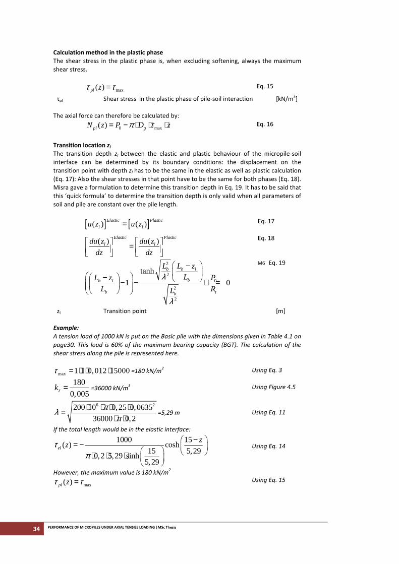
Calculation method in the plastic phase
The shear stress in the plastic phase is, when excluding softening, always the maximum
shear stress.
max( )pl zτ τ= Eq. 15
τpl Shear stress in the plastic phase of pile-soil interaction [kN/m2]
The axial force can therefore be calculated by:
0 max( )pl gN z P D zπ τ= − ⋅ ⋅ ⋅ Eq. 16
Transition location zl
The transition depth zl between the elastic and plastic behaviour of the micropile-soil
interface can be determined by its boundary conditions: the displacement on the
transition point with depth zl has to be the same in the elastic as well as plastic calculation
(Eq. 17): Also the shear stresses in that point have to be the same for both phases (Eq. 18).
Misra gave a formulation to determine this transition depth in Eq. 19. It has to be said that
this ‘quick formula’ to determine the transition depth is only valid when all parameters of
soil and pile are constant over the pile length.
[ ] [ ]( ) ( )Elastic Plastic
l lu z u z= Eq. 17
( ) ( )Elastic Plastic
l ldu z du z
dz dz =
Eq. 18
2
20
2
2
tanh
1 0
b b l
bb l
b tb
L L z
LL z P
L RL
λ
λ
− − − − + =
M6 Eq. 19
zl Transition point [m]
Example:
A tension load of 1000 kN is put on the Basic pile with the dimensions given in Table 4.1 on
page30. This load is 60% of the maximum bearing capacity (BGT). The calculation of the
shear stress along the pile is represented here.
max 1 1 0,012 15000τ = ⋅ ⋅ ⋅ =180 kN/m2
180
0,005kτ = =36000 kN/m
3
6 2200 10 0,25 0,0635
36000 0,2
πλπ
⋅ ⋅ ⋅ ⋅=⋅ ⋅
=5,29 m
If the total length would be in the elastic interface:
1000 15( ) cosh
15 5,290,2 5,29 sinh
5,29
el
zzτ
π
− = − ⋅ ⋅ ⋅
However, the maximum value is 180 kN/m2
max( )pl zτ τ=
Using Eq. 3
Using Figure 4.5
Using Eq. 11
Using Eq. 14
Using Eq. 15
CHAPTER 4| MODELLING AXIALLY LOADED MICROPILES IN TENSION 35
The transition point is at:
2
2
2
2
1515tanh
15 10005,29 151 0
15 1696155,29
l
l
zz
− − − − + =
Using Eq. 19
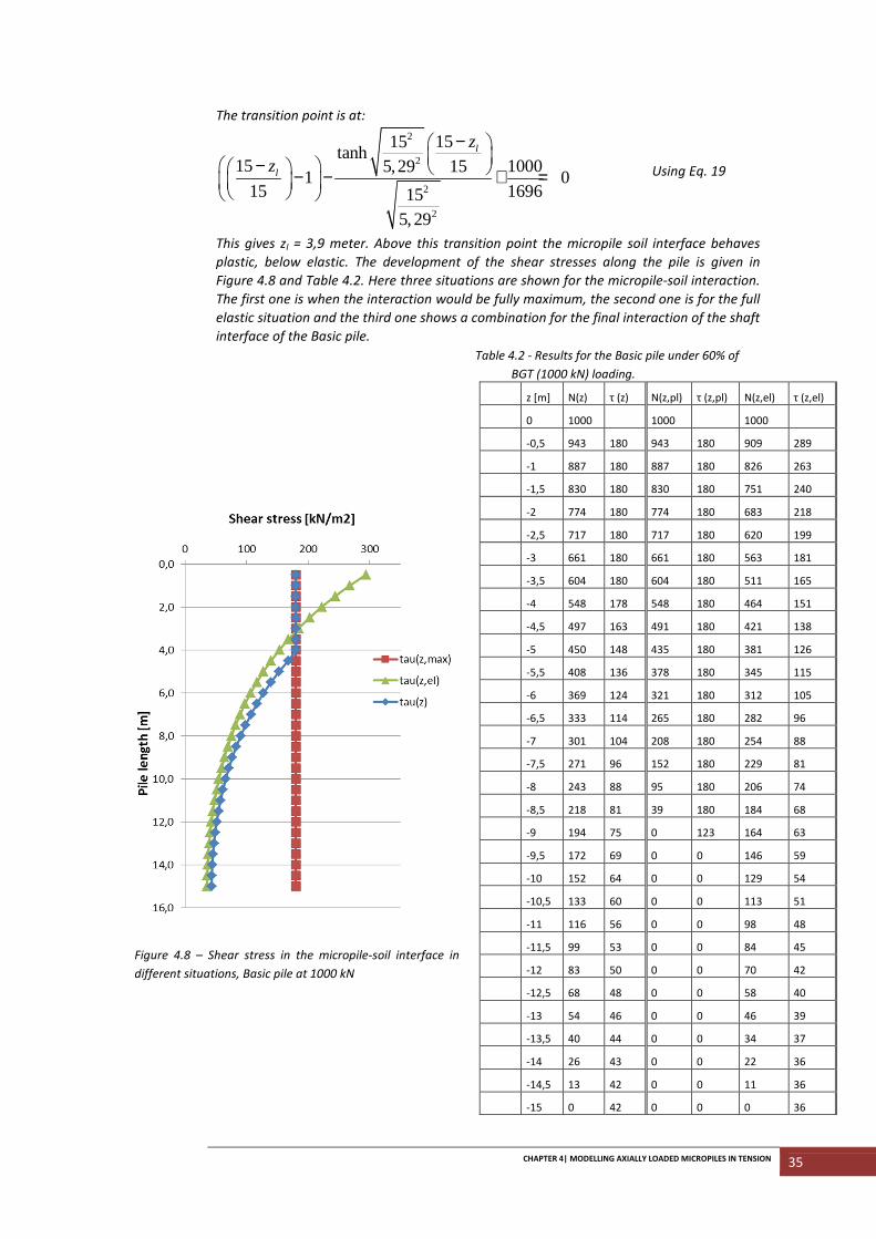
This gives zl = 3,9 meter. Above this transition point the micropile soil interface behaves
plastic, below elastic. The development of the shear stresses along the pile is given in
Figure 4.8 and Table 4.2. Here three situations are shown for the micropile-soil interaction.
The first one is when the interaction would be fully maximum, the second one is for the full
elastic situation and the third one shows a combination for the final interaction of the shaft
interface of the Basic pile.
Table 4.2 - Results for the Basic pile under 60% of
BGT (1000 kN) loading.
Figure 4.8 – Shear stress in the micropile-soil interface in
different situations, Basic pile at 1000 kN
z [m] N(z) τ (z) N(z,pl) τ (z,pl) N(z,el) τ (z,el)
0 1000 1000 1000
-0,5 943 180 943 180 909 289
-1 887 180 887 180 826 263
-1,5 830 180 830 180 751 240
-2 774 180 774 180 683 218
-2,5 717 180 717 180 620 199
-3 661 180 661 180 563 181
-3,5 604 180 604 180 511 165
-4 548 178 548 180 464 151
-4,5 497 163 491 180 421 138
-5 450 148 435 180 381 126
-5,5 408 136 378 180 345 115
-6 369 124 321 180 312 105
-6,5 333 114 265 180 282 96
-7 301 104 208 180 254 88
-7,5 271 96 152 180 229 81
-8 243 88 95 180 206 74
-8,5 218 81 39 180 184 68
-9 194 75 0 123 164 63
-9,5 172 69 0 0 146 59
-10 152 64 0 0 129 54
-10,5 133 60 0 0 113 51
-11 116 56 0 0 98 48
-11,5 99 53 0 0 84 45
-12 83 50 0 0 70 42
-12,5 68 48 0 0 58 40
-13 54 46 0 0 46 39
-13,5 40 44 0 0 34 37
-14 26 43 0 0 22 36
-14,5 13 42 0 0 11 36
-15 0 42 0 0 0 36
36 PERFORMANCE OF MICROPILES UNDER AXIAL TENSILE LOADING |MSc Thesis
4.3.3. Displacement of the pile head The total displacement of the pile head is determined by the lengthening of the pile, the
displacement of the pile tip (due to the upward force) and due to factors of the soil (creep,
heave), presented in Eq. 20. In this case only the single pile is taken into account without
rising of the soil. This calculation is based on the CUR 236.
head length tip creep heaveu u u u u= + + + Eq. 20
uhead Displacement of the pile head [m]
ulength Displacement due to lengthening of the pile [m]
utip Displacement of the pile tip [m]
ucreep Displacement due to creep of the soil [m]
uheave Displacement due to heave of the soil [m]
Elastic deformation of the pile ulength
The local elastic deformation follows from Hooke’s Law (Eq. 21) and the stress definition
(Eq. 22). Combining these gives the deformation on a given depth (Eq. 23). The total
deformation is then the sum of these local deformations: Eq. 24. In this, only the stiffness
of the reinforcement EAs is allowed regarding the safe design of the CUR 236.
Eσ ε= Eq. 21
F
Aσ =
Eq. 22
( )( )
N zz
EAε =
F2b Eq. 23
0
0
( )tot
tot
LL
lengthp
N zu
EAε= = ∫∫
Eq. 24
σ Stress [kN/m2]
A Area [m2]
E Young’s modulus [kN/m2]
Example:
The deformation of the Basic pile under a load of 1000 kN is found by the sum of the
deformation of the elements. The normal force in an element (ʃNi) can be determined by
the average normal force in that element times the length of the element. This is the
normal force used in the lengthening – calculation. For the element at z=6,0 the
deformation is calculated below:
0,5 ((408 369)) / 2)(6,0) 0,0003m
633384ε ⋅ += =
Eq. 24
Displacement of the pile tip utip
The displacement of the pile tip is initiated by the shear stress that is acting in the lowest
element of the pile. Since a deformation is needed to create shear stresses, the tip must
move. To be more accurate a non-linear soil model is used, namely the Hardening Soil
model. This model is visualized in Figure 4.10. The formula corresponding with the figure
(CUR 236 is using P0 and Rt) is re-written for the shear stress (so using τ) to Eq. 25. In this,
the failure ratio and kτ50 determine together the shape of the curve. The kτ50 is the soil
spring stiffness coefficient at 50% of the maximum shear stress and can be calculated by
Eq. 26.
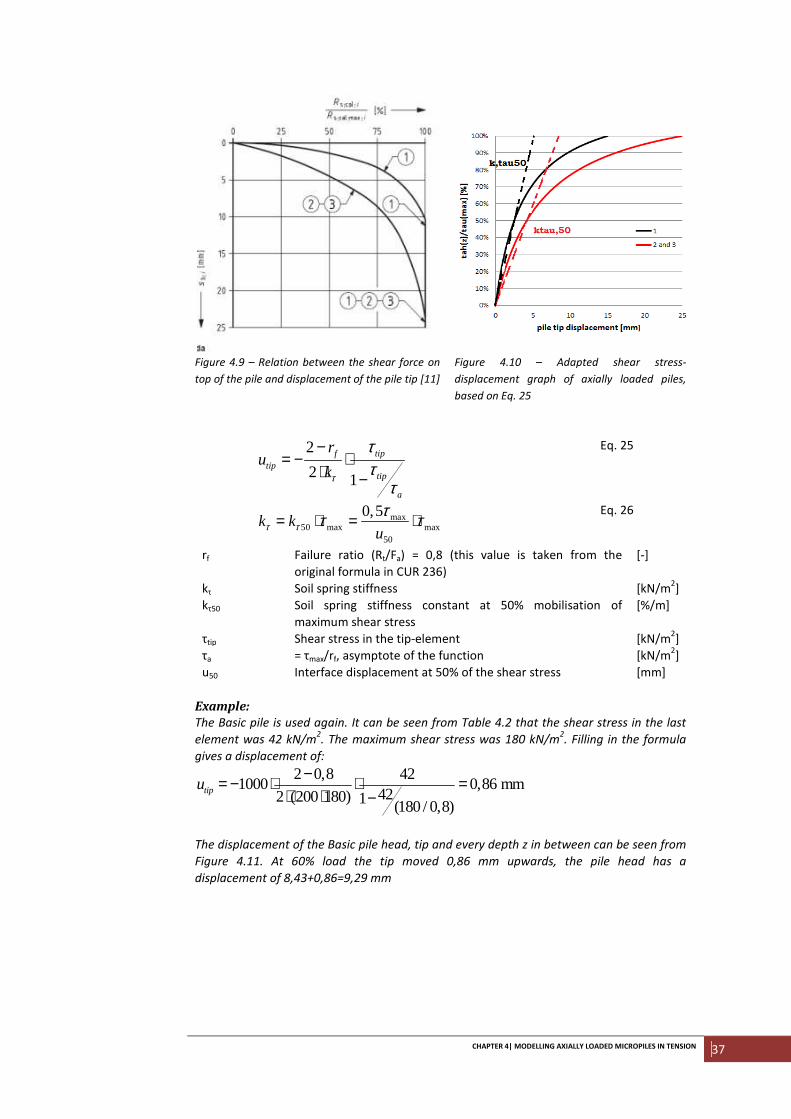
CHAPTER 4| MODELLING AXIALLY LOADED MICROPILES IN TENSION 37
Figure 4.9 – Relation between the shear force on
top of the pile and displacement of the pile tip [11]
Figure 4.10 – Adapted shear stress-
displacement graph of axially loaded piles,
based on Eq. 25
2
2 1
f tiptip
tip
a
ru
kτ
ττ
τ
−= − ⋅
⋅ −
Eq. 25
max
50 max max50
0,5k k
uτ τττ τ= ⋅ = ⋅
Eq. 26
rf Failure ratio (Rt/Fa) = 0,8 (this value is taken from the
original formula in CUR 236)
[-]
kτ Soil spring stiffness [kN/m2]
kτ50 Soil spring stiffness constant at 50% mobilisation of
maximum shear stress
[%/m]
τtip Shear stress in the tip-element [kN/m2]
τa = τmax/rf, asymptote of the function [kN/m2]
u50 Interface displacement at 50% of the shear stress [mm]
Example:
The Basic pile is used again. It can be seen from Table 4.2 that the shear stress in the last
element was 42 kN/m2. The maximum shear stress was 180 kN/m
2. Filling in the formula
gives a displacement of:
2 0,8 421000 0,86 mm
422 (200 180)1 (180 / 0,8)tipu
−= − ⋅ ⋅ =⋅ ⋅ −
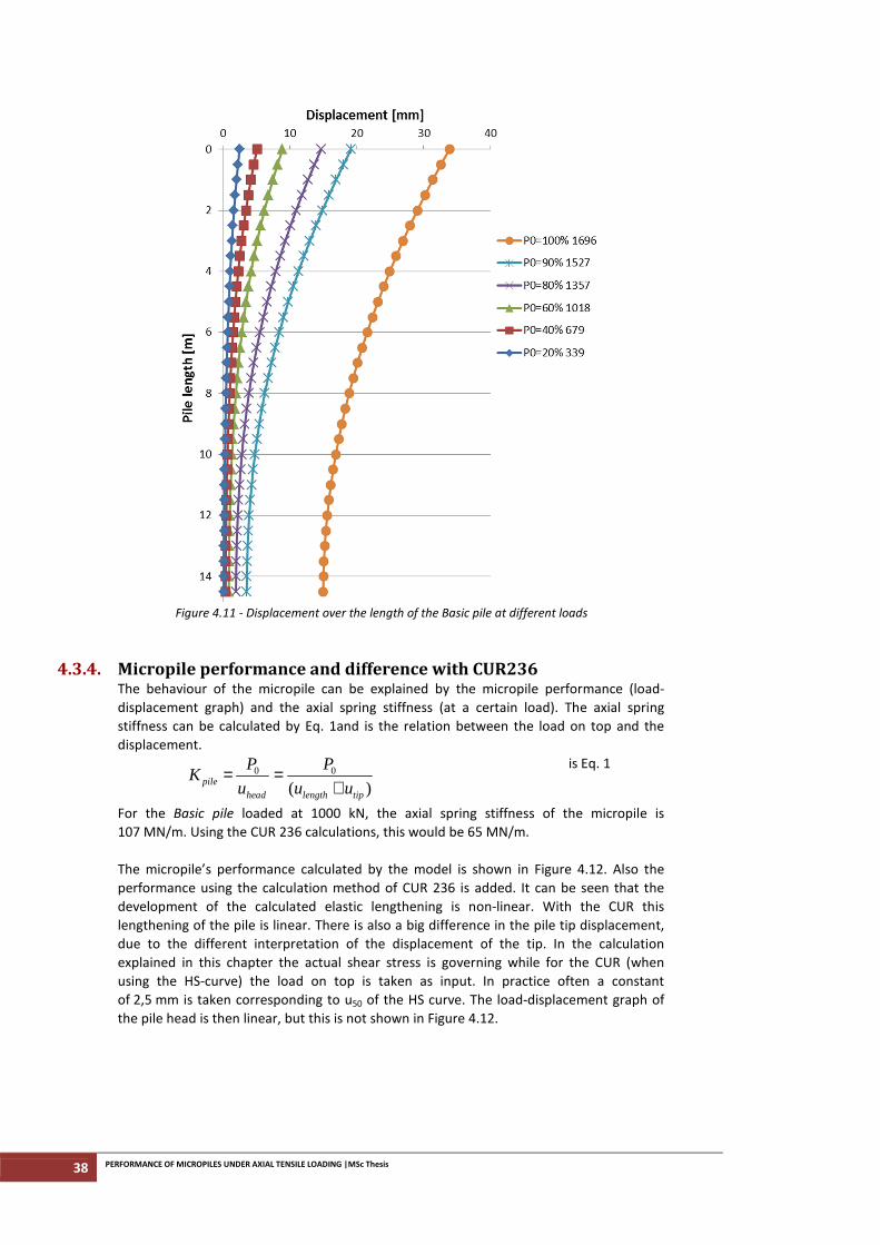
The displacement of the Basic pile head, tip and every depth z in between can be seen from
Figure 4.11. At 60% load the tip moved 0,86 mm upwards, the pile head has a
displacement of 8,43+0,86=9,29 mm
38 PERFORMANCE OF MICROPILES UNDER AXIAL TENSILE LOADING |MSc Thesis
Figure 4.11 - Displacement over the length of the Basic pile at different loads
4.3.4. Micropile performance and difference with CUR236 The behaviour of the micropile can be explained by the micropile performance (load-
displacement graph) and the axial spring stiffness (at a certain load). The axial spring
stiffness can be calculated by Eq. 1and is the relation between the load on top and the
displacement.
0 0
( )pilehead length tip
P PK
u u u= =
+
is Eq. 1
For the Basic pile loaded at 1000 kN, the axial spring stiffness of the micropile is
107 MN/m. Using the CUR 236 calculations, this would be 65 MN/m.
The micropile’s performance calculated by the model is shown in Figure 4.12. Also the
performance using the calculation method of CUR 236 is added. It can be seen that the
development of the calculated elastic lengthening is non-linear. With the CUR this
lengthening of the pile is linear. There is also a big difference in the pile tip displacement,
due to the different interpretation of the displacement of the tip. In the calculation
explained in this chapter the actual shear stress is governing while for the CUR (when
using the HS-curve) the load on top is taken as input. In practice often a constant
of 2,5 mm is taken corresponding to u50 of the HS curve. The load-displacement graph of
the pile head is then linear, but this is not shown in Figure 4.12.
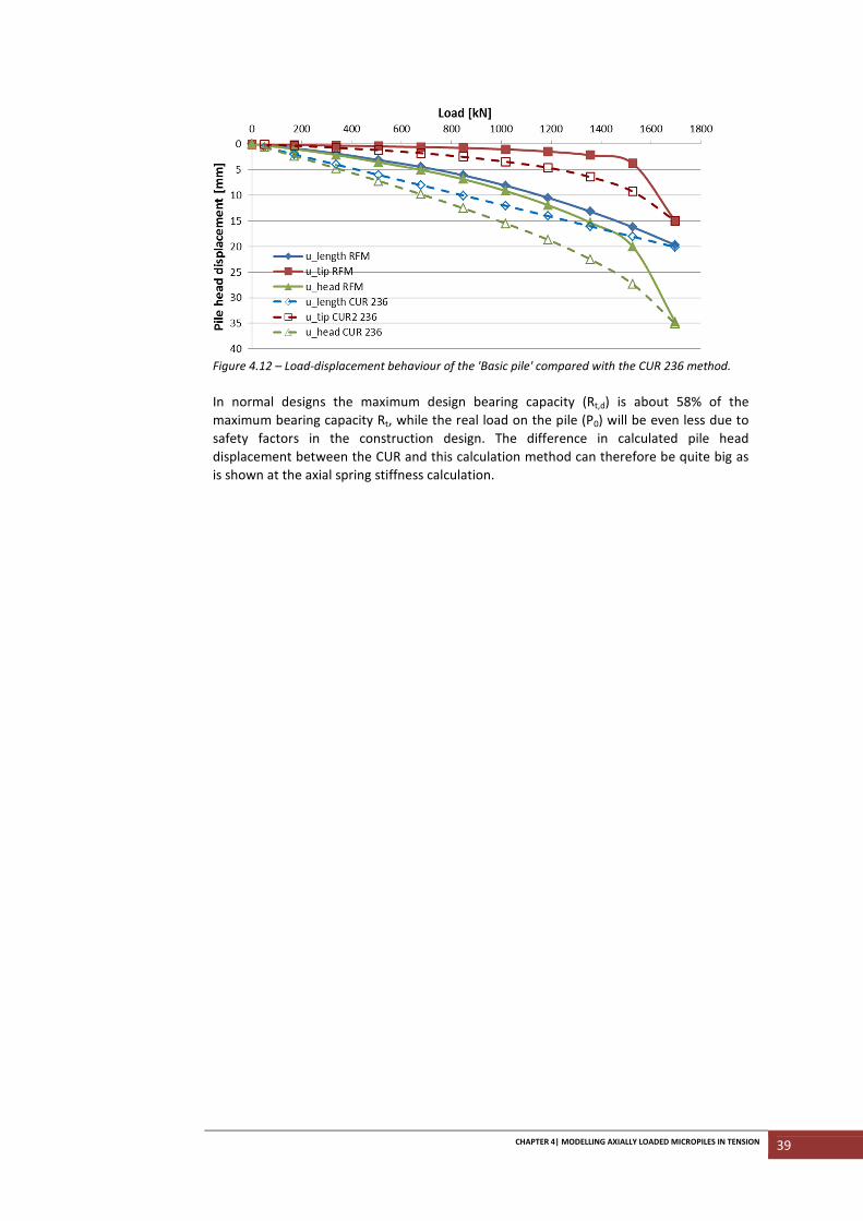
CHAPTER 4| MODELLING AXIALLY LOADED MICROPILES IN TENSION 39
Figure 4.12 – Load-displacement behaviour of the 'Basic pile' compared with the CUR 236 method.
In normal designs the maximum design bearing capacity (Rt,d) is about 58% of the
maximum bearing capacity Rt, while the real load on the pile (P0) will be even less due to
safety factors in the construction design. The difference in calculated pile head
displacement between the CUR and this calculation method can therefore be quite big as
is shown at the axial spring stiffness calculation.

40 PERFORMANCE OF MICROPILES UNDER AXIAL TENSILE LOADING |MSc Thesis
CHAPTER 5| STRUCTURAL BEHAVIOUR 41
5 STRUCTURAL BEHAVIOUR
The stiffness of micropiles is an important parameter in the determination of the pile head
displacement. Both steel reinforcement and grout will contribute to the micropiles’
stiffness. However, it is not just counting up the two material stiffnesses. Due to the
properties of both materials the combined stiffness might vary with execution method,
material strengths and loading condition. Nowadays their composite behaviour is not clear
and only the steel contribution is taken into account. Understanding the combined
behaviour might be of positive influence on the design: adding the stiffness of grout might
double the stiffness of the pile, resulting in a smaller (calculated) displacement of the pile
head.
In this chapter the composite behaviour of the materials under tension loading is
investigated. First a closer look is given to the stress-strain development of the separate
materials, after which the behaviour of the combined materials is discussed. The
behaviour of grout is important in the composite stiffness of the pile. As commonly
known, grout (as well as concrete) can bear high compression loads, but in tension only
small loads and strains due to its brittle behaviour. With its elastic and plastic properties
steel can resist both high compression and tension stresses. Three possible failure modes
can be distinguished in the pile when it is loaded in tension:
- Vertical debonding in the steel-grout interface
- Vertical cracking in the grout, just next to the steel-grout interface
- Horizontal cracking in the grout
Due to its properties a micropile can be considered as a reinforced concrete element. It is
assumed that the load will grab exactly on the vertical axis z and only normal forces are
created in the pile. Bending moments in the grout due to load-transfer in steel-grout and
grout-soil interfaces are assumed to be small and will not be discussed in detail.
Practical research in cracking behaviour of grout in micropiles is very expensive and
difficult. Laboratory testing could be done, but research using field tests to its occurrence
is not often done. The BBRI [22] (Belgium Building Research Institute, research to Ground
Anchors 2004-2008) had an extensive test program of different types of ground anchors
combined with the excavation of these piles. Vertical as well as horizontal strand and
hollow reinforcement-anchors were used in tertiary Brussalian sand, a heterogeneous
clayey sand layer and loam. The anchors were about 11 meter consisting of about 5 meter
bond length. In the free length the reinforcement is surrounded by a plastic casing to
prevent load-transfer.
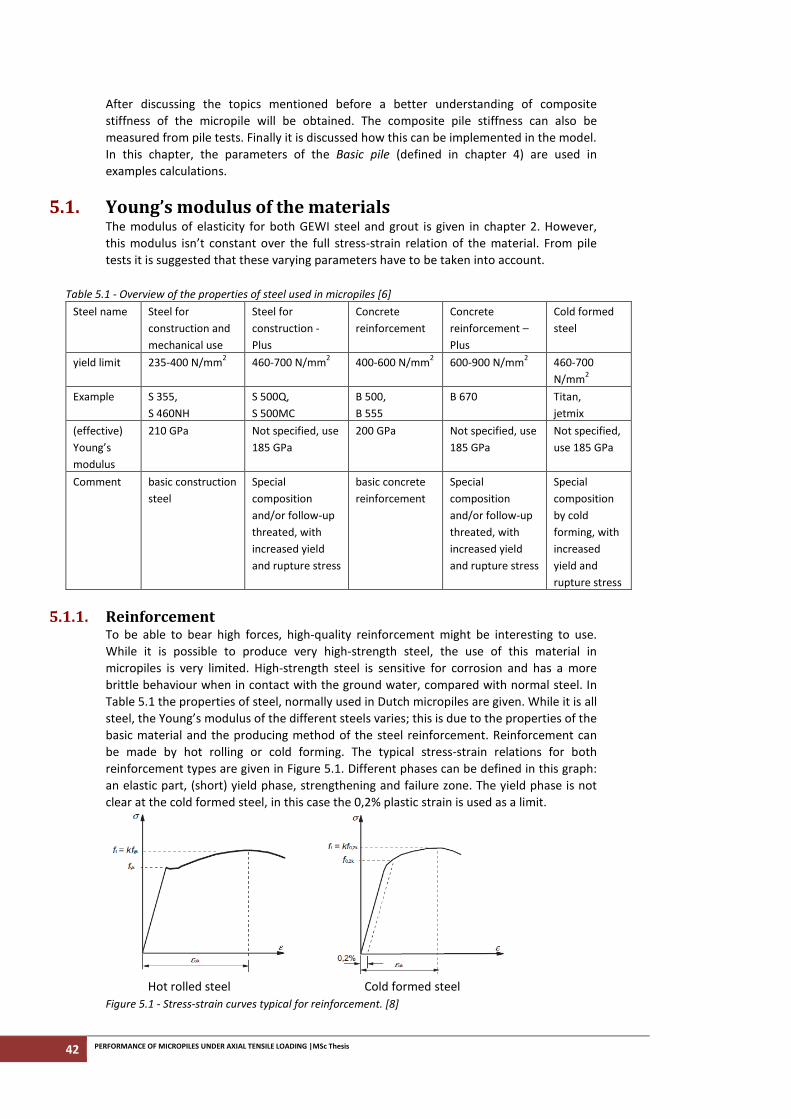
42 PERFORMANCE OF MICROPILES UNDER AXIAL TENSILE LOADING |MSc Thesis
After discussing the topics mentioned before a better understanding of composite
stiffness of the micropile will be obtained. The composite pile stiffness can also be
measured from pile tests. Finally it is discussed how this can be implemented in the model.
In this chapter, the parameters of the Basic pile (defined in chapter 4) are used in
examples calculations.
5.1. Young’s modulus of the materials The modulus of elasticity for both GEWI steel and grout is given in chapter 2. However,
this modulus isn’t constant over the full stress-strain relation of the material. From pile
tests it is suggested that these varying parameters have to be taken into account.
Table 5.1 - Overview of the properties of steel used in micropiles [6]
Steel name
Steel for
construction and
mechanical use
Steel for
construction -
Plus
Concrete
reinforcement
Concrete
reinforcement –
Plus
Cold formed
steel
yield limit 235-400 N/mm2
460-700 N/mm2 400-600 N/mm
2 600-900 N/mm
2 460-700
N/mm2
Example S 355,
S 460NH
S 500Q,
S 500MC
B 500,
B 555
B 670 Titan,
jetmix
(effective)
Young’s
modulus
210 GPa Not specified, use
185 GPa
200 GPa Not specified, use
185 GPa
Not specified,
use 185 GPa
Comment basic construction
steel
Special
composition
and/or follow-up
threated, with
increased yield
and rupture stress
basic concrete
reinforcement
Special
composition
and/or follow-up
threated, with
increased yield
and rupture stress
Special
composition
by cold
forming, with
increased
yield and
rupture stress
5.1.1. Reinforcement To be able to bear high forces, high-quality reinforcement might be interesting to use.
While it is possible to produce very high-strength steel, the use of this material in
micropiles is very limited. High-strength steel is sensitive for corrosion and has a more
brittle behaviour when in contact with the ground water, compared with normal steel. In
Table 5.1 the properties of steel, normally used in Dutch micropiles are given. While it is all
steel, the Young’s modulus of the different steels varies; this is due to the properties of the
basic material and the producing method of the steel reinforcement. Reinforcement can
be made by hot rolling or cold forming. The typical stress-strain relations for both
reinforcement types are given in Figure 5.1. Different phases can be defined in this graph:
an elastic part, (short) yield phase, strengthening and failure zone. The yield phase is not
clear at the cold formed steel, in this case the 0,2% plastic strain is used as a limit.
Hot rolled steel Cold formed steel
Figure 5.1 - Stress-strain curves typical for reinforcement. [8]
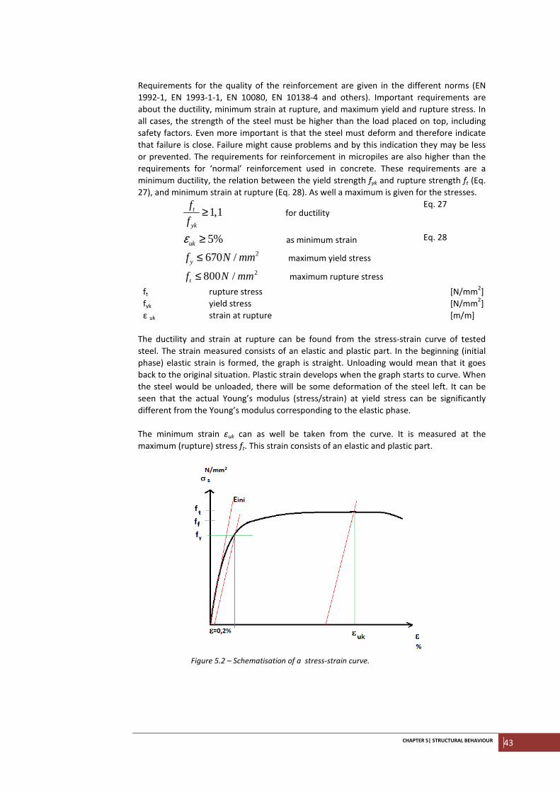
CHAPTER 5| STRUCTURAL BEHAVIOUR 43
Requirements for the quality of the reinforcement are given in the different norms (EN
1992-1, EN 1993-1-1, EN 10080, EN 10138-4 and others). Important requirements are
about the ductility, minimum strain at rupture, and maximum yield and rupture stress. In
all cases, the strength of the steel must be higher than the load placed on top, including
safety factors. Even more important is that the steel must deform and therefore indicate
that failure is close. Failure might cause problems and by this indication they may be less
or prevented. The requirements for reinforcement in micropiles are also higher than the
requirements for ‘normal’ reinforcement used in concrete. These requirements are a
minimum ductility, the relation between the yield strength fyk and rupture strength ft (Eq.
27), and minimum strain at rupture (Eq. 28). As well a maximum is given for the stresses.
1,1t
yk
f
f≥ for ductility
Eq. 27
5%ukε ≥ as minimum strain Eq. 28
2670 /yf N mm≤ maximum yield stress
2800 /tf N mm≤ maximum rupture stress
ft rupture stress [N/mm2]
fyk yield stress [N/mm2]
ε uk strain at rupture [m/m]
The ductility and strain at rupture can be found from the stress-strain curve of tested
steel. The strain measured consists of an elastic and plastic part. In the beginning (initial
phase) elastic strain is formed, the graph is straight. Unloading would mean that it goes
back to the original situation. Plastic strain develops when the graph starts to curve. When
the steel would be unloaded, there will be some deformation of the steel left. It can be
seen that the actual Young’s modulus (stress/strain) at yield stress can be significantly
different from the Young’s modulus corresponding to the elastic phase.
The minimum strain εuk can as well be taken from the curve. It is measured at the
maximum (rupture) stress ft. This strain consists of an elastic and plastic part.
Figure 5.2 – Schematisation of a stress-strain curve.
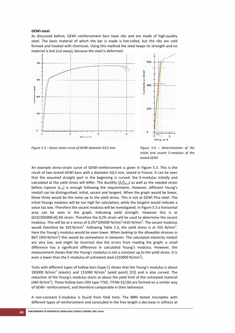
44 PERFORMANCE OF MICROPILES UNDER AXIAL TENSILE LOADING |MSc Thesis
GEWI-steel
As discussed before, GEWI reinforcement bars have ribs and are made of high-quality
steel. The basic material of which the bar is made is hot-rolled, but the ribs are cold
formed and treated with chemicals. Using this method the steel keeps its strength and no
material is lost (cut away), because the steel is deformed.
Figure 5.3 – Stress strain curve of GEWI diameter 63,5 mm Figure 5.4 – Determination of the
initial and secant E-modulus of the
tested GEWI
An example stress-strain curve of GEWI-reinforcement is given in Figure 5.3. This is the
result of two tested GEWI bars with a diameter 63,5 mm, tested in France. It can be seen
that the assumed straight part in the beginning is curved: the E-modulus initially and
calculated at the yield stress will differ. The ductility (ft/fp0,2) as well as the needed strain
before rupture (εuk) is enough following the requirements. However, different Young’s
moduli can be distinguished: initial, secant and tangent. When the graph would be linear,
these three would be the same up to the yield stress. This is not at GEWI Plus steel. The
initial Youngs modulus will be too high for calculation, while the tangent would indicate a
value too low. Therefore the secant modulus will be investigated. In Figure 5.3 a horizontal
area can be seen in the graph, indicating yield strength. However this is at
(610/205000=)0,3% strain. Therefore the 0,2% strain will be used to determine the secant
modulus. This will be at a stress of 0,2%*205000 N/mm2=410 N/mm
2. The secant modulus
would therefore be 103 N/mm2. Following Table 2.3, the yield stress is at 555 N/mm
2.
Here the Young’s modulus would be even lower. When looking to the allowable stresses in
BGT (450 N/mm2) this would be somewhere in between. The calculated elasticity moduli
are very low, and might be incorrect due the errors from reading the graph: a small
difference has a significant difference in calculated Young’s modulus. However, the
measurement shows that the Young’s modulus is not a constant up to the yield stress. It is
even a lower than the E-modulus of untreated steel (210000 N/mm2).
Tests with different types of hollow bars (type C) shows that the Young’s modulus is about
185000 N/mm2 (elastic) and 115000 N/mm
2 (yield point) [23] and is also curved. The
reduction of the Young’s modulus starts at about the yield limit of the untreated material
(460 N/mm2). These hollow bars (DSI type T76S, TITAN 52/26) are formed on a similar way
of GEWI- reinforcement, and therefore comparable in their behaviour.
A non-constant E-modulus is found from field tests. The BBRI tested micropiles with
different types of reinforcement and concluded in the free length a decrease in stifness at
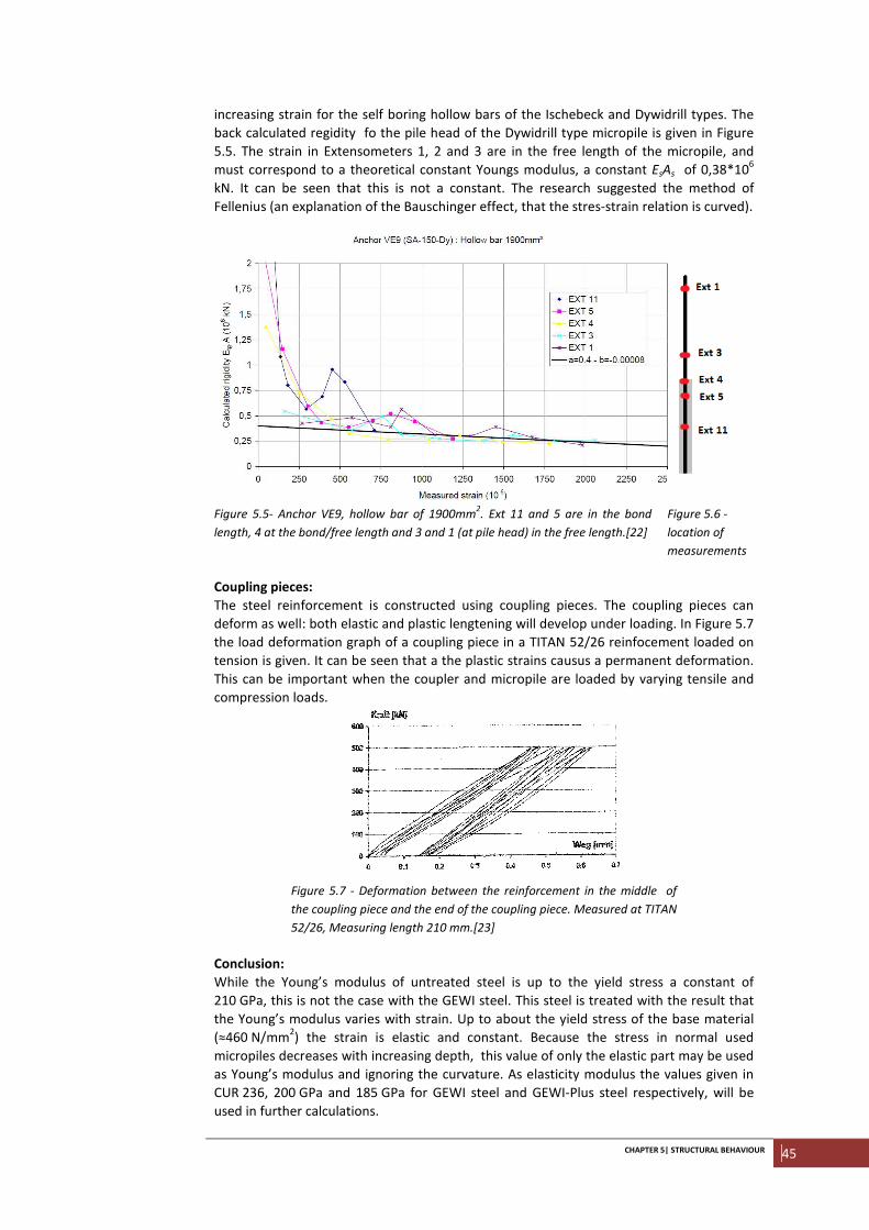
CHAPTER 5| STRUCTURAL BEHAVIOUR 45
increasing strain for the self boring hollow bars of the Ischebeck and Dywidrill types. The
back calculated regidity fo the pile head of the Dywidrill type micropile is given in Figure
5.5. The strain in Extensometers 1, 2 and 3 are in the free length of the micropile, and
must correspond to a theoretical constant Youngs modulus, a constant EsAs of 0,38*106
kN. It can be seen that this is not a constant. The research suggested the method of
Fellenius (an explanation of the Bauschinger effect, that the stres-strain relation is curved).
Figure 5.5- Anchor VE9, hollow bar of 1900mm2. Ext 11 and 5 are in the bond
length, 4 at the bond/free length and 3 and 1 (at pile head) in the free length.[22]
Figure 5.6 -
location of
measurements
Coupling pieces:
The steel reinforcement is constructed using coupling pieces. The coupling pieces can
deform as well: both elastic and plastic lengtening will develop under loading. In Figure 5.7
the load deformation graph of a coupling piece in a TITAN 52/26 reinfocement loaded on
tension is given. It can be seen that a the plastic strains causus a permanent deformation.
This can be important when the coupler and micropile are loaded by varying tensile and
compression loads.
Figure 5.7 - Deformation between the reinforcement in the middle of
the coupling piece and the end of the coupling piece. Measured at TITAN
52/26, Measuring length 210 mm.[23]
Conclusion:
While the Young’s modulus of untreated steel is up to the yield stress a constant of
210 GPa, this is not the case with the GEWI steel. This steel is treated with the result that
the Young’s modulus varies with strain. Up to about the yield stress of the base material
(≈460 N/mm2) the strain is elastic and constant. Because the stress in normal used
micropiles decreases with increasing depth, this value of only the elastic part may be used
as Young’s modulus and ignoring the curvature. As elasticity modulus the values given in
CUR 236, 200 GPa and 185 GPa for GEWI steel and GEWI-Plus steel respectively, will be
used in further calculations.
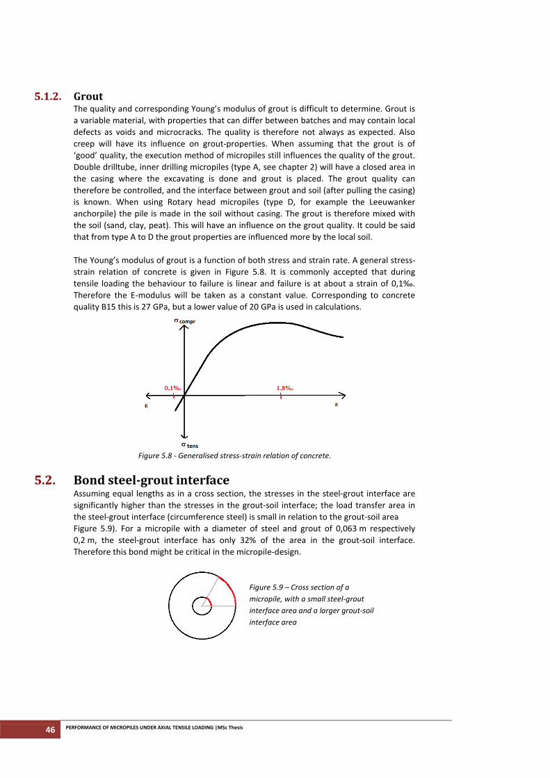
46 PERFORMANCE OF MICROPILES UNDER AXIAL TENSILE LOADING |MSc Thesis
5.1.2. Grout The quality and corresponding Young’s modulus of grout is difficult to determine. Grout is
a variable material, with properties that can differ between batches and may contain local
defects as voids and microcracks. The quality is therefore not always as expected. Also
creep will have its influence on grout-properties. When assuming that the grout is of
‘good’ quality, the execution method of micropiles still influences the quality of the grout.
Double drilltube, inner drilling micropiles (type A, see chapter 2) will have a closed area in
the casing where the excavating is done and grout is placed. The grout quality can
therefore be controlled, and the interface between grout and soil (after pulling the casing)
is known. When using Rotary head micropiles (type D, for example the Leeuwanker
anchorpile) the pile is made in the soil without casing. The grout is therefore mixed with
the soil (sand, clay, peat). This will have an influence on the grout quality. It could be said
that from type A to D the grout properties are influenced more by the local soil.
The Young’s modulus of grout is a function of both stress and strain rate. A general stress-
strain relation of concrete is given in Figure 5.8. It is commonly accepted that during
tensile loading the behaviour to failure is linear and failure is at about a strain of 0,1‰.
Therefore the E-modulus will be taken as a constant value. Corresponding to concrete
quality B15 this is 27 GPa, but a lower value of 20 GPa is used in calculations.
Figure 5.8 - Generalised stress-strain relation of concrete.
5.2. Bond steel-grout interface Assuming equal lengths as in a cross section, the stresses in the steel-grout interface are
significantly higher than the stresses in the grout-soil interface; the load transfer area in
the steel-grout interface (circumference steel) is small in relation to the grout-soil area
Figure 5.9). For a micropile with a diameter of steel and grout of 0,063 m respectively
0,2 m, the steel-grout interface has only 32% of the area in the grout-soil interface.
Therefore this bond might be critical in the micropile-design.
Figure 5.9 – Cross section of a
micropile, with a small steel-grout
interface area and a larger grout-soil
interface area
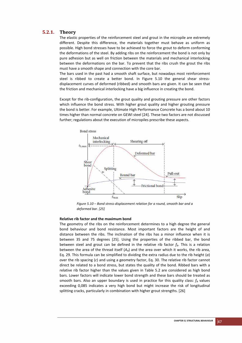
CHAPTER 5| STRUCTURAL BEHAVIOUR 47
5.2.1. Theory The elastic properties of the reinforcement steel and grout in the micropile are extremely
different. Despite this difference, the materials together must behave as uniform as
possible. High bond stresses have to be achieved to force the grout to deform conforming
the deformations of the steel. By adding ribs on the reinforcement the bond is not only by
pure adhesion but as well on friction between the materials and mechanical interlocking
between the deformations on the bar. To prevent that the ribs crush the grout the ribs
must have a smooth shape and connection with the core bar.
The bars used in the past had a smooth shaft surface, but nowadays most reinforcement
steel is ribbed to create a better bond. In Figure 5.10 the general shear stress-
displacement curves of deformed (ribbed) and smooth bars are given. It can be seen that
the friction and mechanical interlocking have a big influence in creating the bond.
Except for the rib-configuration, the grout quality and grouting pressure are other factors
which influence the bond stress. With higher grout quality and higher grouting pressure
the bond is better. For example, Ultimate High Performance Concrete has a bond about 10
times higher than normal concrete on GEWI steel [24]. These two factors are not discussed
further; regulations about the execution of micropiles prescribe these aspects.
Figure 5.10 – Bond stress-displacement relation for a round, smooth bar and a
deformed bar. [25]
Relative rib factor and the maximum bond
The geometry of the ribs on the reinforcement determines to a high degree the general
bond behaviour and bond resistance. Most important factors are the height of and
distance between the ribs. The inclination of the ribs has a minor influence when it is
between 35 and 75 degrees [25]. Using the properties of the ribbed bar, the bond
between steel and grout can be defined in the relative rib factor fR. This is a relation
between the area of the thread itself (AR) and the area over which it works, the rib area,
Eq. 29. This formula can be simplified to dividing the extra radius due to the rib height (a)
over the rib spacing (c) and using a geometry factor, Eq. 30. The relative rib factor cannot
direct be related to a bond stress, but states the quality of the bond. Ribbed bars with a
relative rib factor higher than the values given in Table 5.2 are considered as high bond
bars. Lower factors will indicate lower bond strength and these bars should be treated as
smooth bars. Also an upper boundary is used in practice for this quality class: fR values
exceeding 0,085 indicates a very high bond but might increase the risk of longitudinal
splitting cracks, particularly in combination with higher grout strengths. [26]
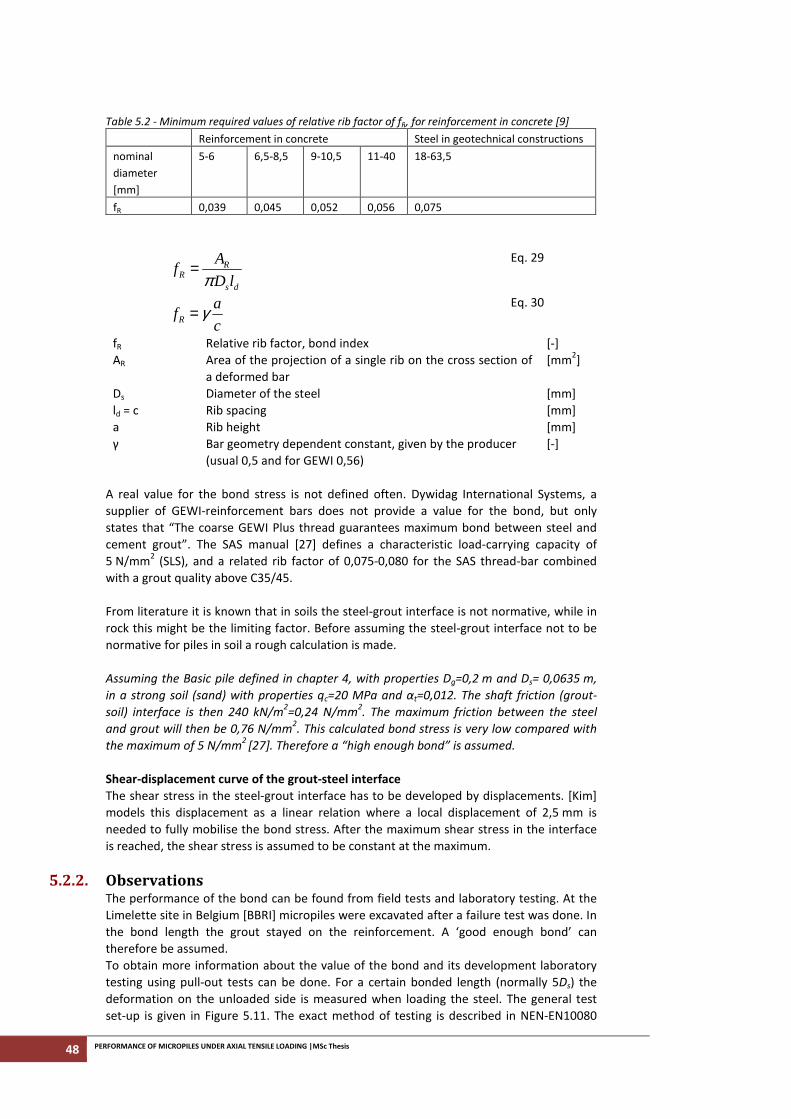
48 PERFORMANCE OF MICROPILES UNDER AXIAL TENSILE LOADING |MSc Thesis
Table 5.2 - Minimum required values of relative rib factor of fR, for reinforcement in concrete [9]
Reinforcement in concrete Steel in geotechnical constructions
nominal
diameter
[mm]
5-6 6,5-8,5 9-10,5 11-40 18-63,5
fR 0,039 0,045 0,052 0,056 0,075
R
Rs d
Af
D lπ=
Eq. 29
R
af
cγ=
Eq. 30
fR Relative rib factor, bond index [-]
AR Area of the projection of a single rib on the cross section of
a deformed bar
[mm2]
Ds Diameter of the steel [mm]
ld = c Rib spacing [mm]
a Rib height [mm]
γ Bar geometry dependent constant, given by the producer
(usual 0,5 and for GEWI 0,56)
[-]
A real value for the bond stress is not defined often. Dywidag International Systems, a
supplier of GEWI-reinforcement bars does not provide a value for the bond, but only
states that “The coarse GEWI Plus thread guarantees maximum bond between steel and
cement grout”. The SAS manual [27] defines a characteristic load-carrying capacity of
5 N/mm2 (SLS), and a related rib factor of 0,075-0,080 for the SAS thread-bar combined
with a grout quality above C35/45.
From literature it is known that in soils the steel-grout interface is not normative, while in
rock this might be the limiting factor. Before assuming the steel-grout interface not to be
normative for piles in soil a rough calculation is made.
Assuming the Basic pile defined in chapter 4, with properties Dg=0,2 m and Ds= 0,0635 m,
in a strong soil (sand) with properties qc=20 MPa and αt=0,012. The shaft friction (grout-
soil) interface is then 240 kN/m2=0,24 N/mm
2. The maximum friction between the steel
and grout will then be 0,76 N/mm2. This calculated bond stress is very low compared with
the maximum of 5 N/mm2
[27]. Therefore a “high enough bond” is assumed.
Shear-displacement curve of the grout-steel interface
The shear stress in the steel-grout interface has to be developed by displacements. [Kim]
models this displacement as a linear relation where a local displacement of 2,5 mm is
needed to fully mobilise the bond stress. After the maximum shear stress in the interface
is reached, the shear stress is assumed to be constant at the maximum.
5.2.2. Observations The performance of the bond can be found from field tests and laboratory testing. At the
Limelette site in Belgium [BBRI] micropiles were excavated after a failure test was done. In
the bond length the grout stayed on the reinforcement. A ‘good enough bond’ can
therefore be assumed.
To obtain more information about the value of the bond and its development laboratory
testing using pull-out tests can be done. For a certain bonded length (normally 5Ds) the
deformation on the unloaded side is measured when loading the steel. The general test
set-up is given in Figure 5.11. The exact method of testing is described in NEN-EN10080
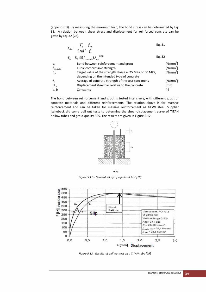
CHAPTER 5| STRUCTURAL BEHAVIOUR 49
(appendix D). By measuring the maximum load, the bond stress can be determined by Eq.
31. A relation between shear stress and displacement for reinforced concrete can be
given by Eq. 32 [28].
25a cm
dmc
F f
d fτ
π=
Eq. 31
0,18, ,0,38b cm cube r cf Uτ = Eq. 32
τb Bond between reinforcement and grout [N/mm2]
fcm,cube Cubic compressive strength [N/mm2]
fcm Target value of the strength class i.e. 25 MPa or 50 MPa,
depending on the intended type of concrete
[N/mm2]
fc Average of concrete strength of the test specimens [N/mm2]
Ur,c Displacement steel bar relative to the concrete [mm]
a, b Constants [-]
The bond between reinforcement and grout is tested intensively, with different grout or
concrete materials and different reinforcements. The relation above is for massive
reinforcement and can be taken for massive reinforcement as GEWI steel. Supplier
Ischebeck did some pull out tests to determine the shear-displacement curve of TITAN
hollow tubes and grout quality B25. The results are given in Figure 5.12.
Figure 5.11 – General set up of a pull-out test [28]
Figure 5.12 - Results of pull-out test on a TITAN tube [29]
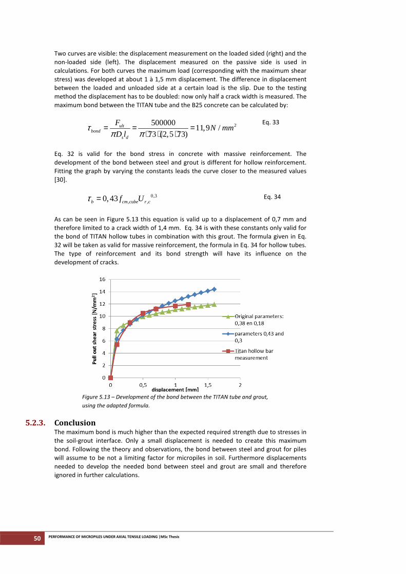
50 PERFORMANCE OF MICROPILES UNDER AXIAL TENSILE LOADING |MSc Thesis
Two curves are visible: the displacement measurement on the loaded sided (right) and the
non-loaded side (left). The displacement measured on the passive side is used in
calculations. For both curves the maximum load (corresponding with the maximum shear
stress) was developed at about 1 à 1,5 mm displacement. The difference in displacement
between the loaded and unloaded side at a certain load is the slip. Due to the testing
method the displacement has to be doubled: now only half a crack width is measured. The
maximum bond between the TITAN tube and the B25 concrete can be calculated by:
250000011,9 /
73 (2,5 73)ult
bonds d
FN mm
D lτ
π π= = =
⋅ ⋅ ⋅
Eq. 33
Eq. 32 is valid for the bond stress in concrete with massive reinforcement. The
development of the bond between steel and grout is different for hollow reinforcement.
Fitting the graph by varying the constants leads the curve closer to the measured values
[30].
0,3, ,0,43b cm cube r cf Uτ = Eq. 34
As can be seen in Figure 5.13 this equation is valid up to a displacement of 0,7 mm and
therefore limited to a crack width of 1,4 mm. Eq. 34 is with these constants only valid for
the bond of TITAN hollow tubes in combination with this grout. The formula given in Eq.
32 will be taken as valid for massive reinforcement, the formula in Eq. 34 for hollow tubes.
The type of reinforcement and its bond strength will have its influence on the
development of cracks.
Figure 5.13 – Development of the bond between the TITAN tube and grout,
using the adapted formula.
5.2.3. Conclusion The maximum bond is much higher than the expected required strength due to stresses in
the soil-grout interface. Only a small displacement is needed to create this maximum
bond. Following the theory and observations, the bond between steel and grout for piles
will assume to be not a limiting factor for micropiles in soil. Furthermore displacements
needed to develop the needed bond between steel and grout are small and therefore
ignored in further calculations.
CHAPTER 5| STRUCTURAL BEHAVIOUR 51
5.3. Vertical cracking The stresses transferred through the steel and the steel-grout interfaces have to be
transferred to the grout-soil interface. Due to the cylindrical shape the stress in the grout
is therefore the largest in the area around the reinforcement. When the bond between
steel and grout is not normative in pile failure, the stress in the grout next to the ribs is
high. A vertical crack might develop parallel to the steel. When this crack reaches the grout
surface corrosion might be expected. From experience with reinforced concrete it is
known that vertical cracks don’t evolve easy when the grout shell is thicker than 1 to 1,5
times the diameter of the reinforcement [26]. Grout is not as well controlled as concrete,
this experience might therefor not be valid for micropiles. However, when cracking
happens the width should be small enough to prevent corrosion of the reinforcement.
At the BBRI research in Limelette some longitudinal fissures are observed. Not only the
free length but in the upper 2 out of 4 m bond length as well. This was in both
reinforcement-types of piles. In these experiments a drill bit with a smaller diameter than
normal was used. The grout cover was only one times the diameter of the reinforcement.
The grout cover in micropiles is normally more than two times the diameter of steel.
Therefore it will be assumed that for these types no vertical cracks will occur or at least
that these cracks do not reach the grout surface. The steel would therefore be sufficiently
enough for corrosion.
5.4. Horizontal cracking The formation of horizontal cracks is expected to be of importance on the stiffness of
micropiles. When the grout fully contributes to the combined stiffness, this might double
the axial stiffness of the micropile, compared with when it isn’t taken into account at all.
The tension-strain of grout is very small, about 0,1 ‰, and it can therefore only bear small
tension forces. When assuming that all forces are taken by the grout, the critical force for
the cracking of the grout would be:
, ,cr g g cr g gN E Aε= Eq. 35
εg,cr Strain at which grout starts to crack [m/m]
Ncr,g Normal force at which the grout starts to crack in the pile,
determined by only the grout
[N]
Applying this to the Basic pile, the critical force would be 56 kN. This is a very low value
and would be for grout only. In reality the micropile can be considered as a reinforced
element loaded in tension. The steel influences the force at which the grout starts cracking
and a higher normal force is expected before cracking.
Eurocode 2 prescribes a limit crack width of 0,1 mm for prestressed reinforced concrete
elements. It is assumed that when the crack width exceeds 0,2 mm corrosion might be
expected at micropiles [26]. When this maximum is not exceeded the grout layer will
prevent the reinforcement for corrosion of the reinforcement during loading conditions.
For extreme conditions (aggressive culture) this norm might be different.
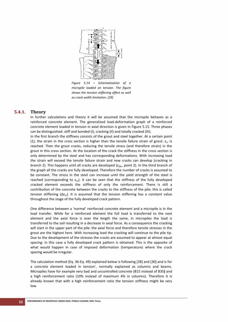
52 PERFORMANCE OF MICROPILES UNDER AXIAL TENSILE LOADING |MSc Thesis
Figure 5.14 – Schematisation of a
micropile loaded on tension. The figure
shows the tension stiffening effect as well
as crack width limitation. [29]
5.4.1. Theory In further calculations and theory it will be assumed that the micropile behaves as a
reinforced concrete element. The generalized load-deformation graph of a reinforced
concrete element loaded in tension in axial direction is given in Figure 5.15. Three phases
can be distinguished: stiff and bonded (I), cracking (II) and totally cracked (III).
In the first branch the stiffness consists of the grout and steel together. At a certain point
(1), the strain in the cross section is higher than the tensile failure strain of grout: εcr is
reached. Then the grout cracks, reducing the tensile stress (and therefore strain) in the
grout in this cross section. At the location of the crack the stiffness in the cross section is
only determined by the steel and has corresponding deformations. With increasing load
the strain will exceed the tensile failure strain and new cracks can develop (cracking in
branch 2). This happens until all cracks are developed (εfdc, point 2). In the third branch of
the graph all the cracks are fully developed. Therefore the number of cracks is assumed to
be constant. The stress in the steel can increase until the yield strength of the steel is
reached (corresponding to εsy). It can be seen that the stiffness of the fully developed
cracked element exceeds the stiffness of only the reinforcement. There is still a
contribution of the concrete between the cracks to the stiffness of the pile; this is called
tension stiffening (Δεts). It is assumed that the tension stiffening has a constant value
throughout the stage of the fully developed crack pattern.
One difference between a ‘normal’ reinforced concrete element and a micropile is in the
load transfer. While for a reinforced element the full load is transferred to the next
element and the axial force is over the length the same, in micropiles the load is
transferred to the soil resulting in a decrease in axial force. As a consequence the cracking
will start in the upper part of the pile: the axial force and therefore tensile stresses in the
grout are the highest here. With increasing load the cracking will continue to the pile tip.
Due to the development of the stresses the cracks are assumed to appear at almost equal
spacing: in this case a fully developed crack pattern is obtained. This is the opposite of
what would happen in case of imposed deformation (temperature) where the crack
spacing would be irregular.
The calculation method (Eq. 36-Eq. 49) explained below is following [28] and [30] and is for
a concrete element loaded in tension’, normally explained as columns and beams.
Micropiles have for example very bad and uncontrolled concrete (B15 instead of B35) and
a high reinforcement ratio (10% instead of maximum 4% in columns). Therefore it is
already known that with a high reinforcement ratio the tension stiffness might be very
low.
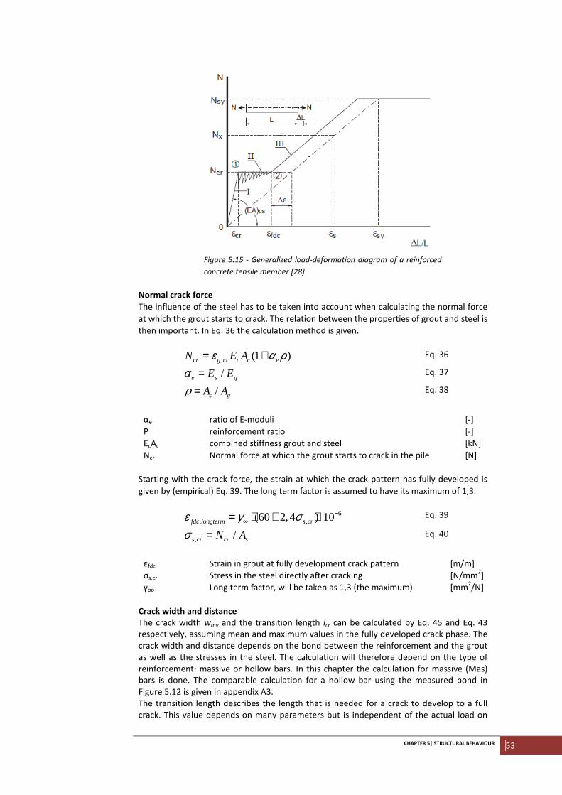
CHAPTER 5| STRUCTURAL BEHAVIOUR 53
Figure 5.15 - Generalized load-deformation diagram of a reinforced
concrete tensile member [28]
Normal crack force
The influence of the steel has to be taken into account when calculating the normal force
at which the grout starts to crack. The relation between the properties of grout and steel is
then important. In Eq. 36 the calculation method is given.
, (1 )cr g cr c c eN E Aε α ρ= + Eq. 36
/e s gE Eα = Eq. 37
/s gA Aρ = Eq. 38
αe ratio of E-moduli [-]
Ρ reinforcement ratio [-]
EcAc combined stiffness grout and steel [kN]
Ncr Normal force at which the grout starts to crack in the pile [N]
Starting with the crack force, the strain at which the crack pattern has fully developed is
given by (empirical) Eq. 39. The long term factor is assumed to have its maximum of 1,3.
6, ,(60 2,4 ) 10fdc longterm s crε γ σ −
∞= ⋅ + ⋅ Eq. 39
, /s cr cr sN Aσ = Eq. 40
εfdc Strain in grout at fully development crack pattern [m/m]
σs,cr Stress in the steel directly after cracking [N/mm2]
γoo Long term factor, will be taken as 1,3 (the maximum) [mm2/N]
Crack width and distance
The crack width wmv and the transition length lcr can be calculated by Eq. 45 and Eq. 43
respectively, assuming mean and maximum values in the fully developed crack phase. The
crack width and distance depends on the bond between the reinforcement and the grout
as well as the stresses in the steel. The calculation will therefore depend on the type of
reinforcement: massive or hollow bars. In this chapter the calculation for massive (Mas)
bars is done. The comparable calculation for a hollow bar using the measured bond in
Figure 5.12 is given in appendix A3.
The transition length describes the length that is needed for a crack to develop to a full
crack. This value depends on many parameters but is independent of the actual load on
54 PERFORMANCE OF MICROPILES UNDER AXIAL TENSILE LOADING |MSc Thesis
the pile. From practice it is known that in reinforced elements cracks will occur between 2
(average) and 3,7 (maximum) times the concrete cover thickness. The crack distance will
therefore be 2 to 3,7 times the cover plus the length which is needed to create a full crack
(Eq. 43).
( )0,852
,
0,42 1s cr
mo ecm cube s
Dw
f E
σ α ρρ
= ⋅ ⋅ +
Eq. 41a
Mas
,
1,8 mo sm
s cr
w El
σ=
Eq. 42a
Mas
, 2cr ave g ml c l= +
,max 3,7cr g ml c l= +
Eq. 43a
Eq. 43b
0,60cr ctmfσ = Eq. 44
wmo Mean crack width at not fully developed crack phase [mm]
σcr Concrete tensile strength at which cracking occurs [N/mm2]
lm
Transition length at fully developed crack phase [mm]
lst Transition length at not fully developed crack phase [mm]
lcr, ave Average crack distance [mm]
lcr, mac Maximum crack distance [mm]
fck Cylinder compressive strength [N/mm2]
Ds Diameter of the steel reinforcement [mm]
cg Grout cover [mm]
The crack width can be calculated with Eq. 45 and depends on the actual stresses; the
stresses in a crack have to be taken by the steel and the pile will deform on this location by
the steel elasticity. This is a linear relation. Due to corrosion protection-regulations the
crack width has a limit. For reinforced concrete elements this limit is 0,1 mm [8], for
micropiles a crack width of 0,2 mm is assumed go give probems with durabilty [26].To
calculate the crack with the permanent (normal) situation has to be taken into account, in
SLS. Therefore the average water level has to be taken into account instead of the highest
water level. The expected steel stress at normal conditions is therefore lower than the
maximum. Normally a factor of about 1,3 is used to take into account high water level, so
the maximum allowable load in SLS depends on the minimum of Eq. 46a and Eq. 46b.
( ),, ,0,5cr ave
mv ave s s crs
lw
Eσ σ= −
Eq. 45a
( ),max,max ,0,5cr
mv s s crs
lw
Eσ σ= −
Eq. 45 b
, 1,3s y
d steelAs
A fR
γ=
⋅
,,2
0,9
1,3s t
d steelBm
A fR
γ⋅=⋅
Eq. 46a
Eq. 46b
wmv ave
Average crack width at fully developed crack phase [mm]
wmv, max
Maximum crack width at fully developed crack phase [mm]
σs Stress in the steel at which cracking occurs [N/mm2]
γs
Material factor for reinforcement steel = 1,15 [-]
γm,2
Material factor for the strength of the treat = 1,25 [-]
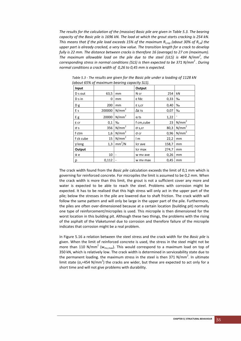
CHAPTER 5| STRUCTURAL BEHAVIOUR 55
The results for the calculation of the (massive) Basic pile are given in Table 5.3. The bearing
capacity of the Basic pile is 1696 kN. The load at which the grout starts cracking is 254 kN.
This means that if the pile load exceeds 15% of the maximum Rt,rep (about 30% of Rt,d) the
upper part is already cracked, a very low value. The transition length for a crack to develop
fully is 22 mm. The distance between cracks is therefore 16 (average) to 27 cm (maximum).
The maximum allowable load on the pile due to the steel (ULS) is 484 N/mm2, the
corresponding stress in normal conditions (SLS) is then expected to be 371 N/mm2
. During
normal conditions a crack width of 0,26 to 0,45 mm is expected.
Table 5.3 - The results are given for the Basic pile under a loading of 1128 kN
(about 65% of maximum bearing capacity SLS).
Input Output
D s out 63,5 mm N cr 254 kN
D s in 0 mm ε fdc 0,33 ‰
D g 200 mm ε s,cr 0,40 ‰
E s 200000 N/mm2 ∆ε ts 0,07 ‰
E g 20000 N/mm2 α ts 1,22 -
ε cr 0,1 ‰ f cm,cube 23 N/mm2
σ s 356 N/mm2 σ s,cr 80,3 N/mm
2
f ctm 1,6 N/mm2 σ cr 0,96 N/mm
2
f ck cube 15 N/mm2 l m 22,2 mm
γ long 1,3 mm2/N lcr ave 158,7 mm
Output lcr max 274,7 mm
α e 10 - w mv ave 0,26 mm
ρ 0,112 - w mv max 0,45 mm
The crack width found from the Basic pile calculation exceeds the limit of 0,1 mm which is
governing for reinforced concrete. For micropiles the limit is assumed to be 0,2 mm. When
the crack width is more than this limit, the grout is not a sufficient cover any more and
water is expected to be able to reach the steel. Problems with corrosion might be
expected. It has to be realised that this high stress will only act in the upper part of the
pile; below the stresses in the pile are lowered due to shaft friction. The crack width will
follow the same pattern and will only be large in the upper part of the pile. Furthermore,
the piles are often over-dimensioned because at a certain location (building pit) normally
one type of reinforcement/micropiles is used. This micropile is then dimensioned for the
worst location in this building pit. Although these two things, the problems with the rising
of the asphalt of the Vlaketunnel due to corrosion and therefore failure of the micropile
indicates that corrosion might be a real problem.
In Figure 5.16 a relation between the steel stress and the crack width for the Basic pile is
given. When the limit of reinforced concrete is used, the stress in the steel might not be
more than 110 N/mm2 (wmv,max). This would correspond to a maximum load on top of
350 kN, which is relatively low. The crack width is determined in serviceability state due to
the permanent loading. the maximum stress in the steel is then 371 N/mm2. In ultimate
limit state (σs=454 N/mm2) the cracks are wider, but these are expected to act only for a
short time and will not give problems with durability.
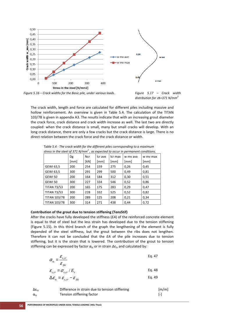
56 PERFORMANCE OF MICROPILES UNDER AXIAL TENSILE LOADING |MSc Thesis
Figure 5.16 – Crack widths for the Basic pile, under various loads. Figure 5.17 – Crack width
distribution for σs=371 N/mm2
The crack width, length and force are calculated for different piles including massive and
hollow reinforcement. An overview is given in Table 5.4. The calculation of the TITAN
103/78 is given in appendix A3. The results indicate that with an increasing grout diameter
the crack force, crack distance and crack width increase as well. The last two are directly
coupled: when the crack distance is small, many but small cracks will develop. With an
long crack distance, there are only a few cracks but the crack distance is large. There is no
direct relation between the crack force and the crack distance or width.
Table 5.4 - The crack width for the different piles corresponding to a maximum
stress in the steel of 371 N/mm2 , as expected to occur in permanent conditions.
Dg
[mm]
Ncr
[kN]
lcr ave
[mm]
lcr max
[mm]
w mv ave
[mm]
w mv max
[mm]
GEWI 63,5 200 254 159 275 0,26 0,45
GEWI 63,5 300 291 299 500 0,49 0,81
GEWI 50 200 164 184 312 0,30 0,51
GEWI 50 300 227 334 546 0,52 0,86
TITAN 73/53 200 165 175 283 0,29 0,47
TITAN 73/53 300 228 332 525 0,52 0,82
TITAN 103/78 200 289 125 208 0,21 0,34
TITAN 103/78 300 314 271 438 0,44 0,72
Contribution of the grout due to tension stiffening (TensStif)
After the cracks have fully developed the stiffness (EA) of the reinforced concrete element
is equal to that of steel but the less strain has developed due to the tension stiffening
(Figure 5.15). In this third branch of the graph the lengthening of the element is fully
depended of the steel stiffness, but the grout between the ribs does not lengthen.
Therefore it can not be concluded that the EA of the pile increases due to tension
stiffening, but it is the strain that is lowered. The contribution of the grout to tension
stiffening can be expressed by factor αts or in strain Δεts and calculated by:
,s cr
tsfdc
εα
ε=
Eq. 47
, , /s cr s cr sEε σ= Eq. 48
,ts s cr fdcε ε ε∆ = − Eq. 49
Δεts Difference in strain due to tension stiffening [m/m]
αts Tension stiffening factor [-]
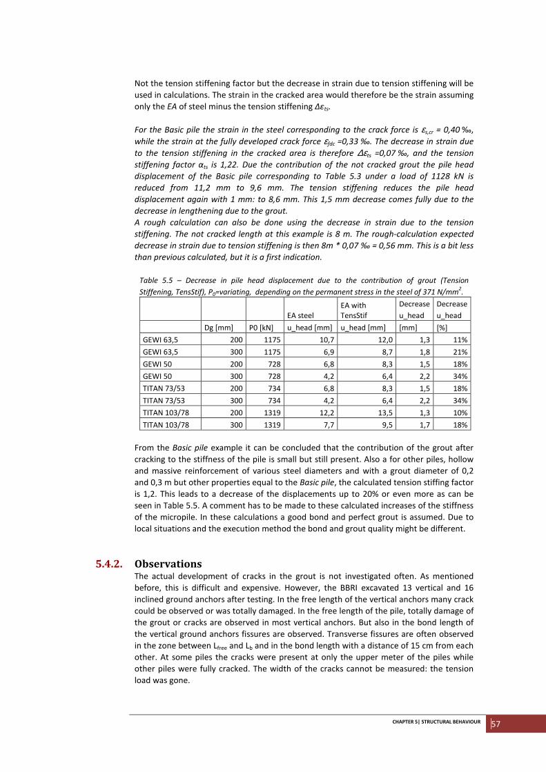
CHAPTER 5| STRUCTURAL BEHAVIOUR 57
Not the tension stiffening factor but the decrease in strain due to tension stiffening will be
used in calculations. The strain in the cracked area would therefore be the strain assuming
only the EA of steel minus the tension stiffening Δεts.
For the Basic pile the strain in the steel corresponding to the crack force is εs,cr = 0,40 ‰,
while the strain at the fully developed crack force εfdc =0,33 ‰. The decrease in strain due
to the tension stiffening in the cracked area is therefore ∆εts =0,07 ‰, and the tension
stiffening factor αts is 1,22. Due the contribution of the not cracked grout the pile head
displacement of the Basic pile corresponding to Table 5.3 under a load of 1128 kN is
reduced from 11,2 mm to 9,6 mm. The tension stiffening reduces the pile head
displacement again with 1 mm: to 8,6 mm. This 1,5 mm decrease comes fully due to the
decrease in lengthening due to the grout.
A rough calculation can also be done using the decrease in strain due to the tension
stiffening. The not cracked length at this example is 8 m. The rough-calculation expected
decrease in strain due to tension stiffening is then 8m * 0,07 ‰ = 0,56 mm. This is a bit less
than previous calculated, but it is a first indication.
Table 5.5 – Decrease in pile head displacement due to the contribution of grout (Tension
Stiffening, TensStif), P0=variating, depending on the permanent stress in the steel of 371 N/mm2.
EA steel
EA with
TensStif
Decrease
u_head
Decrease
u_head
Dg [mm] P0 [kN] u_head [mm] u_head [mm] [mm] [%]
GEWI 63,5 200 1175 10,7 12,0 1,3 11%
GEWI 63,5 300 1175 6,9 8,7 1,8 21%
GEWI 50 200 728 6,8 8,3 1,5 18%
GEWI 50 300 728 4,2 6,4 2,2 34%
TITAN 73/53 200 734 6,8 8,3 1,5 18%
TITAN 73/53 300 734 4,2 6,4 2,2 34%
TITAN 103/78 200 1319 12,2 13,5 1,3 10%
TITAN 103/78 300 1319 7,7 9,5 1,7 18%
From the Basic pile example it can be concluded that the contribution of the grout after
cracking to the stiffness of the pile is small but still present. Also a for other piles, hollow
and massive reinforcement of various steel diameters and with a grout diameter of 0,2
and 0,3 m but other properties equal to the Basic pile, the calculated tension stiffing factor
is 1,2. This leads to a decrease of the displacements up to 20% or even more as can be
seen in Table 5.5. A comment has to be made to these calculated increases of the stiffness
of the micropile. In these calculations a good bond and perfect grout is assumed. Due to
local situations and the execution method the bond and grout quality might be different.
5.4.2. Observations The actual development of cracks in the grout is not investigated often. As mentioned
before, this is difficult and expensive. However, the BBRI excavated 13 vertical and 16
inclined ground anchors after testing. In the free length of the vertical anchors many crack
could be observed or was totally damaged. In the free length of the pile, totally damage of
the grout or cracks are observed in most vertical anchors. But also in the bond length of
the vertical ground anchors fissures are observed. Transverse fissures are often observed
in the zone between Lfree and Lb and in the bond length with a distance of 15 cm from each
other. At some piles the cracks were present at only the upper meter of the piles while
other piles were fully cracked. The width of the cracks cannot be measured: the tension
load was gone.
58 PERFORMANCE OF MICROPILES UNDER AXIAL TENSILE LOADING |MSc Thesis
Figure 5.18 – Crack width measurement at a grout body
180-220 Diameter, 1200mm long reinforced with TITAN
103/51, SWL 1000 kN [29]
In Germany it is standard to do laboratory tests on the materials of micropiles. For a
micropile (steel and grout combination) they measure the crack width at different loading
steps. The results of a test are given in Figure 5.18. It shows that the crack widths are less
than the maximum of 0,1 mm prescribed in the norm. However this was determined at
perfect conditions in the laboratory.
5.5. Combined stiffness In design norms normally the used stiffness for the displacement calculation is the steel
stiffness only (to be conservative). Another assumption could take into account both
materials. The second one would over-estimate the stiffness due to grout cracking. Under
increased loading, the real micropile stiffness will decrease from the steel plus grout
stiffness to only the stiffness of steel, maybe increased by the tension stiffening.
5.5.1. Theory Following from the assumption that debonding and vertical cracking will not happen, only
horizontal cracking will occur. The grout in the Basic pile will crack when the axial force in
the pile is 254 kN and the factor to implement tension stiffening is 1,2. In the cracked area
the strain is therefore lowered by 0,0007 m/m. In the not-cracked area at the lower part of
the pile both steel and grout contribute to the combined stiffness. To see the influence of
the grout to the displacement of the pile head, four situations can be considered (as cab
be seen in Figure 5.19):
• Steel: only the contribution of the EA of steel along the full length (as in chapter 4
and CUR236)
• Steel +Grout Ncr: at the lower part of the pile where no cracks have developed
both steel and grout contributes to the EA of the pile. Where the grout is cracked,
only the contribution of the steel is assumed
• TensStif: at the lower part of the pile where no cracks have developed both steel
and grout contributes to the EA of the pile. Where the grout is cracked, a tension
stiffening factor of 1,2 is assumed.*
• Steel+Grout fully: along the total length both grout and steel contribute to the
stiffness EA. (Due to the low tension capacity of grout this is not realistic, and
calculation is just for imagination)
* Due to the decrease in displacements or local strain, the developed shear stress will a bit
less, resulting in less displacement. This iteration process is not taken into account.
CHAPTER 5| STRUCTURAL BEHAVIOUR 59
a b c d
Figure 5.19 – Schematisation of the four situations: steel(a),
Steel+GroutNcr (b), TensStif (c) and Steel+Grout fully (d).
The results are given in Table 5.6 for the Basic pile under a load of 1000 kN (60% of Rt). It
can be seen that the cracking of the grout has a big influence on the pile performance.
When taking the cracking in to account the differences between no (Steel), only in the
lower part (Steel+GroutNcr) and including tension stiffening (TensStif) on the
performances are small (in mm). Relatively assuming tension stiffening gives still a
reduction of the displacement of 15% when comparing with the ’steel’ situation. In Figure
5.20 the development of the shear stress is given. Again it can be seen that the differences
between cracked grout are small, but the curve corresponding to no cracks is different.
Finally the full load-displacement is given in Figure 5.21. The results for a micropile with
TITAN 103/78 reinforcement are given in appendix A3. At this pile the influence of the
grout to the decrease in pile head displacements is small.
Table 5.6 – Calculated pile head displacement of the Basic pile under a load of 1000 kN (60%), with
different contribution of the grout to the pile's stiffness. *Steel+Grout fully is not realist to occur, so
only added as a fictive situation.
GEWI Steel Steel+GroutNcr TensStif Steel+Grout fully*
u_length 8,4 7,8 6,9 4,7 mm
u_tip 0,8 1,0 1,0 1,4 mm
u_head 9,3 8,8 7,9 6,0 mm
reduction u_head 5% 15% 35%
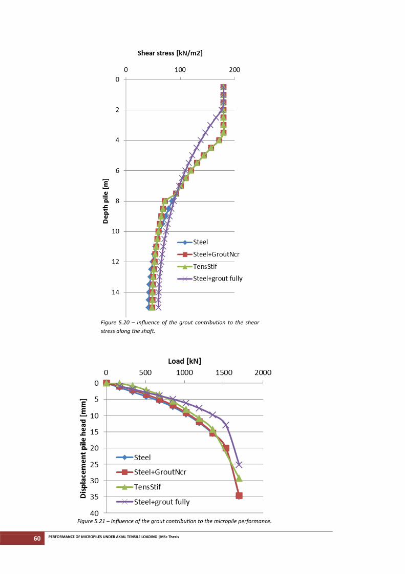
60 PERFORMANCE OF MICROPILES UNDER AXIAL TENSILE LOADING |MSc Thesis
Figure 5.20 – Influence of the grout contribution to the shear
stress along the shaft.
Figure 5.21 – Influence of the grout contribution to the micropile performance.
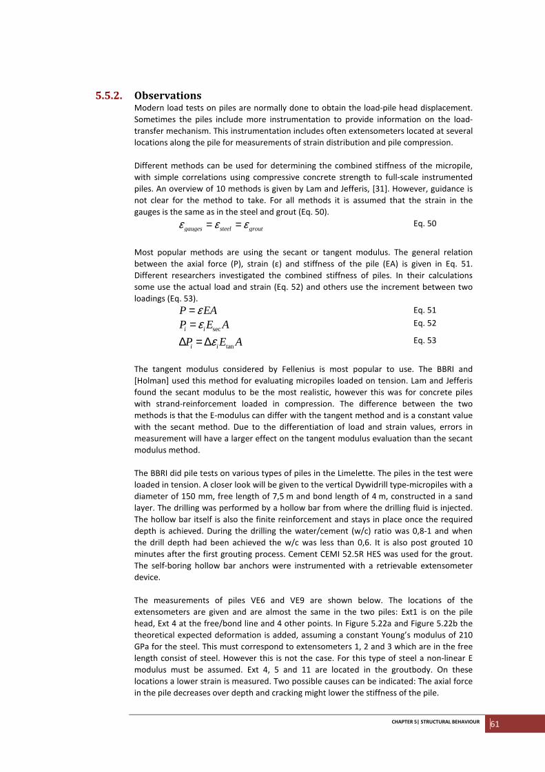
CHAPTER 5| STRUCTURAL BEHAVIOUR 61
5.5.2. Observations Modern load tests on piles are normally done to obtain the load-pile head displacement.
Sometimes the piles include more instrumentation to provide information on the load-
transfer mechanism. This instrumentation includes often extensometers located at several
locations along the pile for measurements of strain distribution and pile compression.
Different methods can be used for determining the combined stiffness of the micropile,
with simple correlations using compressive concrete strength to full-scale instrumented
piles. An overview of 10 methods is given by Lam and Jefferis, [31]. However, guidance is
not clear for the method to take. For all methods it is assumed that the strain in the
gauges is the same as in the steel and grout (Eq. 50).
gauges steel groutε ε ε= = Eq. 50
Most popular methods are using the secant or tangent modulus. The general relation
between the axial force (P), strain (ε) and stiffness of the pile (EA) is given in Eq. 51.
Different researchers investigated the combined stiffness of piles. In their calculations
some use the actual load and strain (Eq. 52) and others use the increment between two
loadings (Eq. 53).
P EAε= Eq. 51
seci iP E Aε= Eq. 52
tani iP E Aε∆ = ∆ Eq. 53
The tangent modulus considered by Fellenius is most popular to use. The BBRI and
[Holman] used this method for evaluating micropiles loaded on tension. Lam and Jefferis
found the secant modulus to be the most realistic, however this was for concrete piles
with strand-reinforcement loaded in compression. The difference between the two
methods is that the E-modulus can differ with the tangent method and is a constant value
with the secant method. Due to the differentiation of load and strain values, errors in
measurement will have a larger effect on the tangent modulus evaluation than the secant
modulus method.
The BBRI did pile tests on various types of piles in the Limelette. The piles in the test were
loaded in tension. A closer look will be given to the vertical Dywidrill type-micropiles with a
diameter of 150 mm, free length of 7,5 m and bond length of 4 m, constructed in a sand
layer. The drilling was performed by a hollow bar from where the drilling fluid is injected.
The hollow bar itself is also the finite reinforcement and stays in place once the required
depth is achieved. During the drilling the water/cement (w/c) ratio was 0,8-1 and when
the drill depth had been achieved the w/c was less than 0,6. It is also post grouted 10
minutes after the first grouting process. Cement CEMI 52.5R HES was used for the grout.
The self-boring hollow bar anchors were instrumented with a retrievable extensometer
device.
The measurements of piles VE6 and VE9 are shown below. The locations of the
extensometers are given and are almost the same in the two piles: Ext1 is on the pile
head, Ext 4 at the free/bond line and 4 other points. In Figure 5.22a and Figure 5.22b the
theoretical expected deformation is added, assuming a constant Young’s modulus of 210
GPa for the steel. This must correspond to extensometers 1, 2 and 3 which are in the free
length consist of steel. However this is not the case. For this type of steel a non-linear E
modulus must be assumed. Ext 4, 5 and 11 are located in the groutbody. On these
locations a lower strain is measured. Two possible causes can be indicated: The axial force
in the pile decreases over depth and cracking might lower the stiffness of the pile.
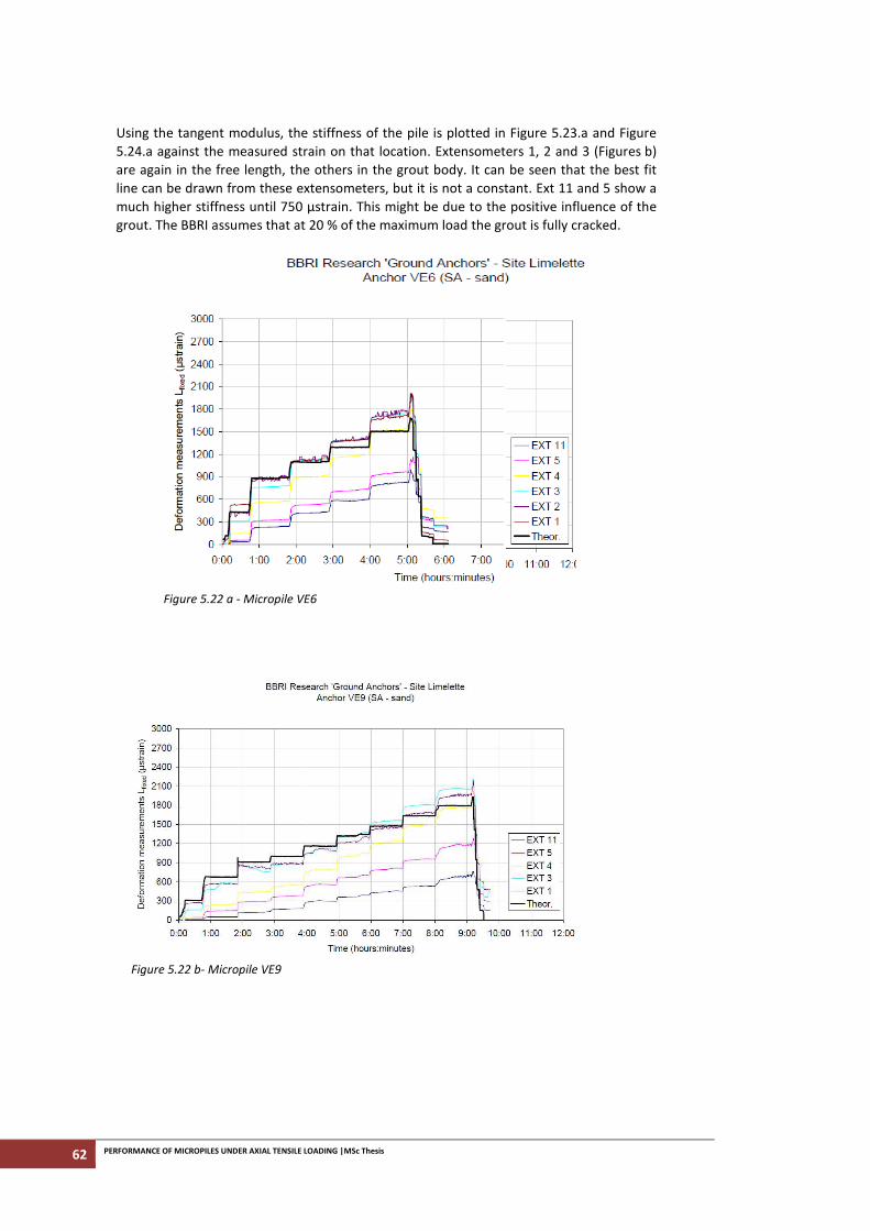
62 PERFORMANCE OF MICROPILES UNDER AXIAL TENSILE LOADING |MSc Thesis
Using the tangent modulus, the stiffness of the pile is plotted in Figure 5.23.a and Figure
5.24.a against the measured strain on that location. Extensometers 1, 2 and 3 (Figures b)
are again in the free length, the others in the grout body. It can be seen that the best fit
line can be drawn from these extensometers, but it is not a constant. Ext 11 and 5 show a
much higher stiffness until 750 μstrain. This might be due to the positive influence of the
grout. The BBRI assumes that at 20 % of the maximum load the grout is fully cracked.
Figure 5.22 a - Micropile VE6
Figure 5.22 b- Micropile VE9
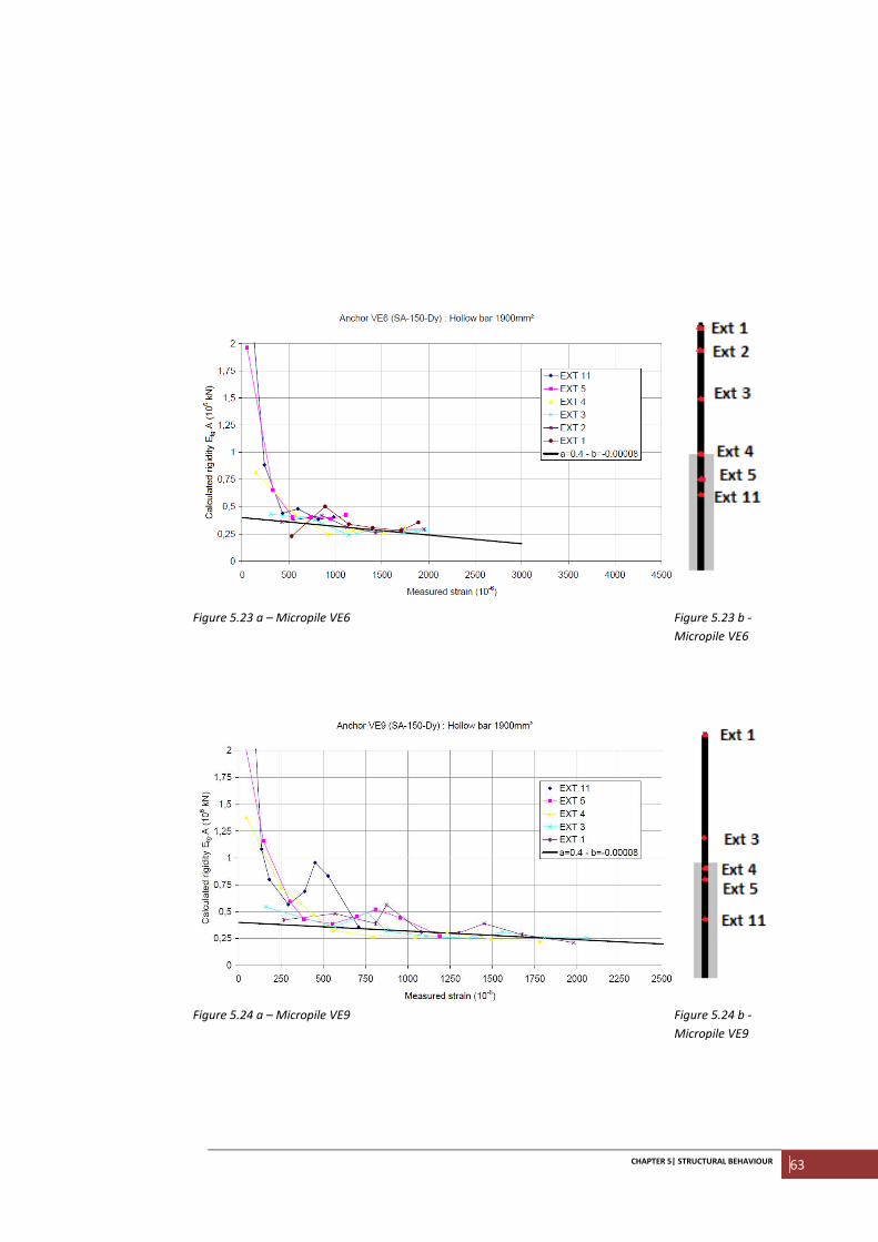
CHAPTER 5| STRUCTURAL BEHAVIOUR 63
Figure 5.23 a – Micropile VE6 Figure 5.23 b -
Micropile VE6
Figure 5.24 a – Micropile VE9 Figure 5.24 b -
Micropile VE9
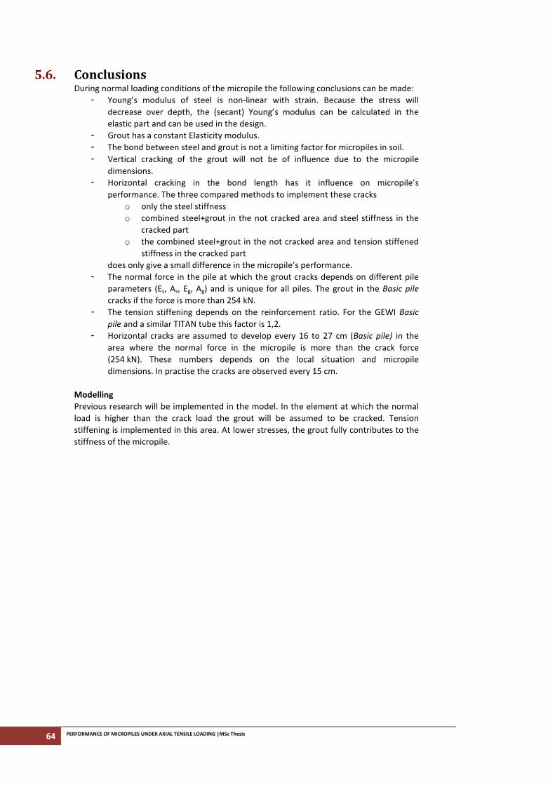
64 PERFORMANCE OF MICROPILES UNDER AXIAL TENSILE LOADING |MSc Thesis
5.6. Conclusions During normal loading conditions of the micropile the following conclusions can be made:
- Young’s modulus of steel is non-linear with strain. Because the stress will
decrease over depth, the (secant) Young’s modulus can be calculated in the
elastic part and can be used in the design.
- Grout has a constant Elasticity modulus.
- The bond between steel and grout is not a limiting factor for micropiles in soil.
- Vertical cracking of the grout will not be of influence due to the micropile
dimensions.
- Horizontal cracking in the bond length has it influence on micropile’s
performance. The three compared methods to implement these cracks
o only the steel stiffness
o combined steel+grout in the not cracked area and steel stiffness in the
cracked part
o the combined steel+grout in the not cracked area and tension stiffened
stiffness in the cracked part
does only give a small difference in the micropile’s performance.
- The normal force in the pile at which the grout cracks depends on different pile
parameters (Es, As, Eg, Ag) and is unique for all piles. The grout in the Basic pile
cracks if the force is more than 254 kN.
- The tension stiffening depends on the reinforcement ratio. For the GEWI Basic
pile and a similar TITAN tube this factor is 1,2.
- Horizontal cracks are assumed to develop every 16 to 27 cm (Basic pile) in the
area where the normal force in the micropile is more than the crack force
(254 kN). These numbers depends on the local situation and micropile
dimensions. In practise the cracks are observed every 15 cm.
Modelling
Previous research will be implemented in the model. In the element at which the normal
load is higher than the crack load the grout will be assumed to be cracked. Tension
stiffening is implemented in this area. At lower stresses, the grout fully contributes to the
stiffness of the micropile.
CHAPTER 6| SOIL BEHAVIOUR 65
6 SOIL BEHAVIOUR
Not only the structural behaviour but also the soil behaviour has its influence on the
micropile performance. In this chapter different aspects will be examined in more detail.
First, the influence of the load direction which might lower the maximum shear stress and
the occurrence of softening which might give the pile a lower maximum capacity are
discussed. Because in chapter 4 a linear elastic-perfectly plastic load-transfer is assumed, it
will be discussed if this linearization has a significant influence on the calculation. Then a
closer look will be given to the soil stiffness coefficient. Finally the implementation of soil
layering in the model is discussed.
Figure 6.1 – Influence of the load direction on the shear stress
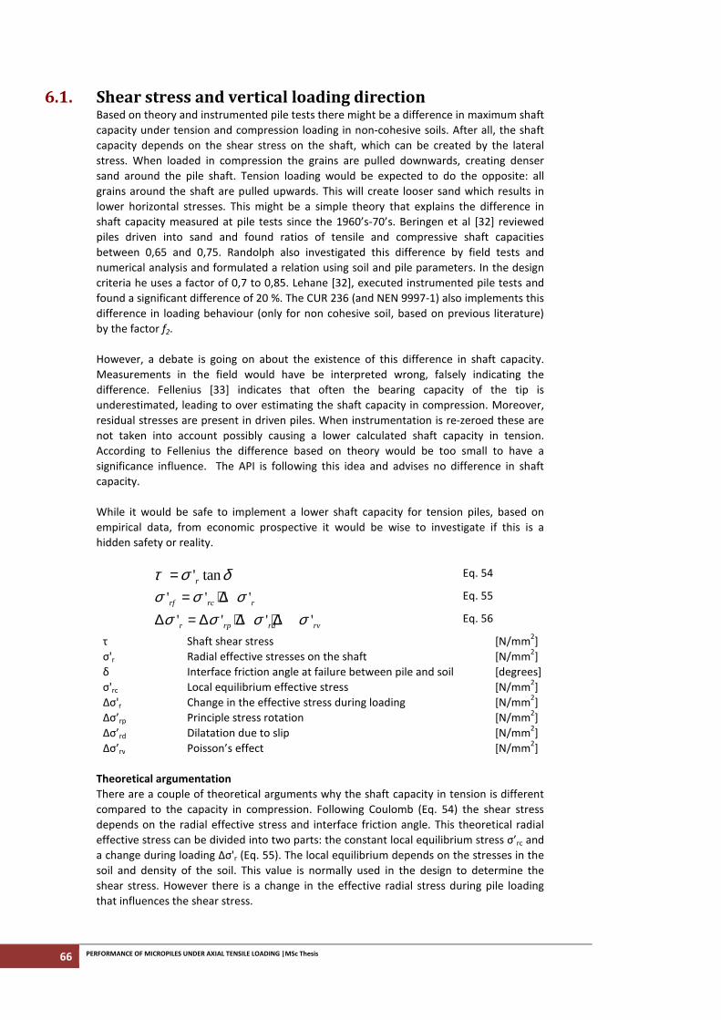
66 PERFORMANCE OF MICROPILES UNDER AXIAL TENSILE LOADING |MSc Thesis
6.1. Shear stress and vertical loading direction Based on theory and instrumented pile tests there might be a difference in maximum shaft
capacity under tension and compression loading in non-cohesive soils. After all, the shaft
capacity depends on the shear stress on the shaft, which can be created by the lateral
stress. When loaded in compression the grains are pulled downwards, creating denser
sand around the pile shaft. Tension loading would be expected to do the opposite: all
grains around the shaft are pulled upwards. This will create looser sand which results in
lower horizontal stresses. This might be a simple theory that explains the difference in
shaft capacity measured at pile tests since the 1960’s-70’s. Beringen et al [32] reviewed
piles driven into sand and found ratios of tensile and compressive shaft capacities
between 0,65 and 0,75. Randolph also investigated this difference by field tests and
numerical analysis and formulated a relation using soil and pile parameters. In the design
criteria he uses a factor of 0,7 to 0,85. Lehane [32], executed instrumented pile tests and
found a significant difference of 20 %. The CUR 236 (and NEN 9997-1) also implements this
difference in loading behaviour (only for non cohesive soil, based on previous literature)
by the factor f2.
However, a debate is going on about the existence of this difference in shaft capacity.
Measurements in the field would have be interpreted wrong, falsely indicating the
difference. Fellenius [33] indicates that often the bearing capacity of the tip is
underestimated, leading to over estimating the shaft capacity in compression. Moreover,
residual stresses are present in driven piles. When instrumentation is re-zeroed these are
not taken into account possibly causing a lower calculated shaft capacity in tension.
According to Fellenius the difference based on theory would be too small to have a
significance influence. The API is following this idea and advises no difference in shaft
capacity.
While it would be safe to implement a lower shaft capacity for tension piles, based on
empirical data, from economic prospective it would be wise to investigate if this is a
hidden safety or reality.
' tanrτ σ δ= Eq. 54
' ' 'rf rc rσ σ σ= + ∆ Eq. 55
' ' ' 'r rp rd rvσ σ σ σ∆ = ∆ + ∆ + ∆ Eq. 56
τ Shaft shear stress [N/mm2]
σ'r Radial effective stresses on the shaft [N/mm2]
δ Interface friction angle at failure between pile and soil [degrees]
σ'rc Local equilibrium effective stress [N/mm2]
Δσ'r Change in the effective stress during loading [N/mm2]
Δσ’rp Principle stress rotation [N/mm2]
Δσ’rd Dilatation due to slip [N/mm2]
Δσ’rv Poisson’s effect [N/mm2]
Theoretical argumentation
There are a couple of theoretical arguments why the shaft capacity in tension is different
compared to the capacity in compression. Following Coulomb (Eq. 54) the shear stress
depends on the radial effective stress and interface friction angle. This theoretical radial
effective stress can be divided into two parts: the constant local equilibrium stress σ’rc and
a change during loading Δσ'r (Eq. 55). The local equilibrium depends on the stresses in the
soil and density of the soil. This value is normally used in the design to determine the
shear stress. However there is a change in the effective radial stress during pile loading
that influences the shear stress.
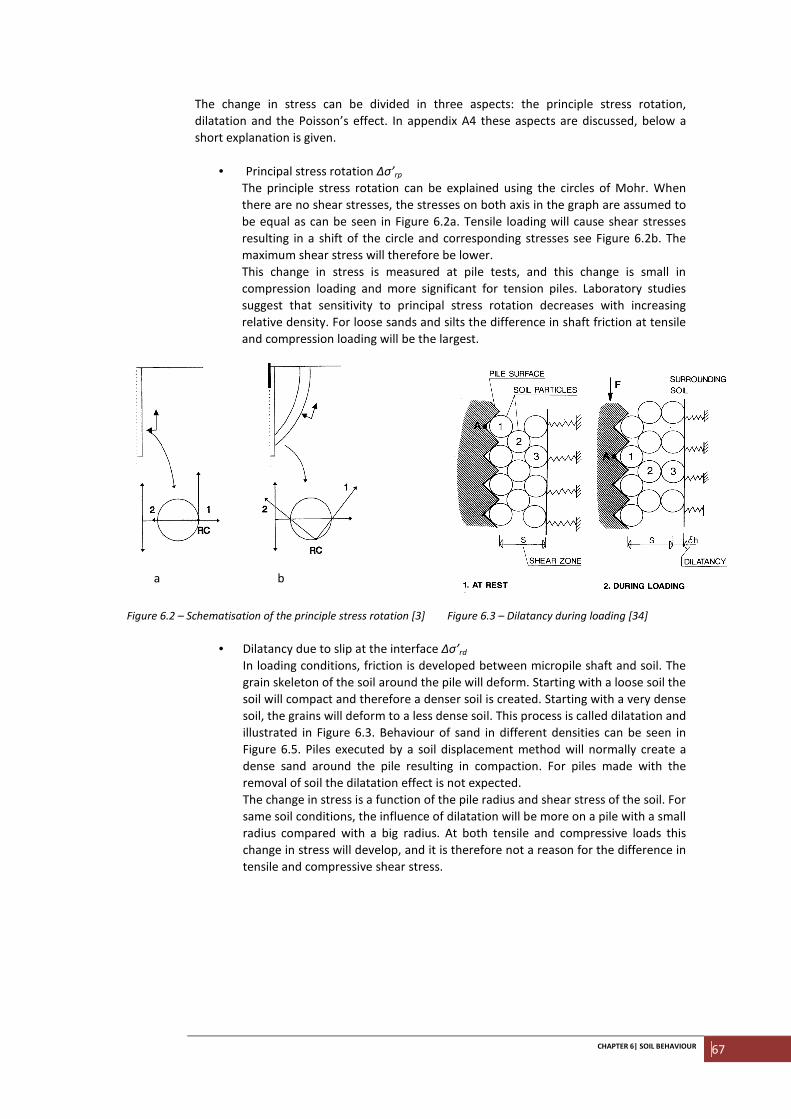
CHAPTER 6| SOIL BEHAVIOUR 67
The change in stress can be divided in three aspects: the principle stress rotation,
dilatation and the Poisson’s effect. In appendix A4 these aspects are discussed, below a
short explanation is given.
• Principal stress rotation Δσ’rp
The principle stress rotation can be explained using the circles of Mohr. When
there are no shear stresses, the stresses on both axis in the graph are assumed to
be equal as can be seen in Figure 6.2a. Tensile loading will cause shear stresses
resulting in a shift of the circle and corresponding stresses see Figure 6.2b. The
maximum shear stress will therefore be lower.
This change in stress is measured at pile tests, and this change is small in
compression loading and more significant for tension piles. Laboratory studies
suggest that sensitivity to principal stress rotation decreases with increasing
relative density. For loose sands and silts the difference in shaft friction at tensile
and compression loading will be the largest.
a b
Figure 6.2 – Schematisation of the principle stress rotation [3] Figure 6.3 – Dilatancy during loading [34]
• Dilatancy due to slip at the interface Δσ’rd
In loading conditions, friction is developed between micropile shaft and soil. The
grain skeleton of the soil around the pile will deform. Starting with a loose soil the
soil will compact and therefore a denser soil is created. Starting with a very dense
soil, the grains will deform to a less dense soil. This process is called dilatation and
illustrated in Figure 6.3. Behaviour of sand in different densities can be seen in
Figure 6.5. Piles executed by a soil displacement method will normally create a
dense sand around the pile resulting in compaction. For piles made with the
removal of soil the dilatation effect is not expected.
The change in stress is a function of the pile radius and shear stress of the soil. For
same soil conditions, the influence of dilatation will be more on a pile with a small
radius compared with a big radius. At both tensile and compressive loads this
change in stress will develop, and it is therefore not a reason for the difference in
tensile and compressive shear stress.
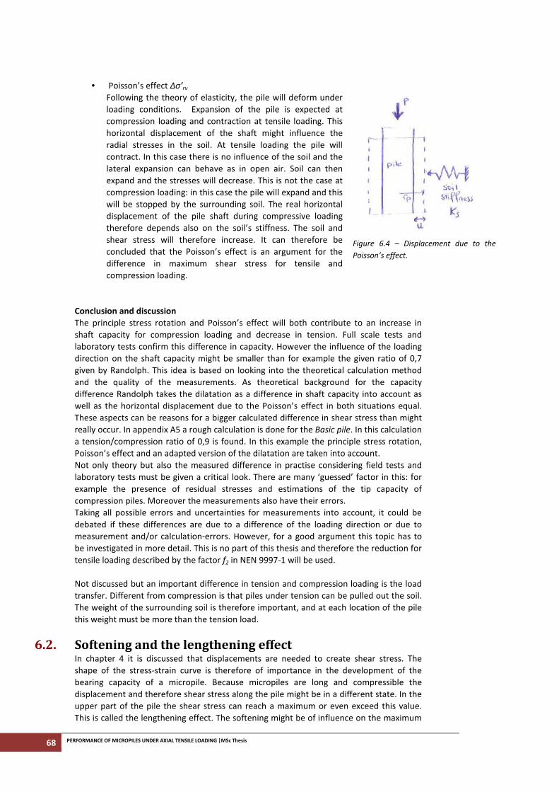
68 PERFORMANCE OF MICROPILES UNDER AXIAL TENSILE LOADING |MSc Thesis
• Poisson’s effect Δσ’rv
Following the theory of elasticity, the pile will deform under
loading conditions. Expansion of the pile is expected at
compression loading and contraction at tensile loading. This
horizontal displacement of the shaft might influence the
radial stresses in the soil. At tensile loading the pile will
contract. In this case there is no influence of the soil and the
lateral expansion can behave as in open air. Soil can then
expand and the stresses will decrease. This is not the case at
compression loading: in this case the pile will expand and this
will be stopped by the surrounding soil. The real horizontal
displacement of the pile shaft during compressive loading
therefore depends also on the soil’s stiffness. The soil and
shear stress will therefore increase. It can therefore be
concluded that the Poisson’s effect is an argument for the
difference in maximum shear stress for tensile and
compression loading.
Figure 6.4 – Displacement due to the
Poisson’s effect.
Conclusion and discussion
The principle stress rotation and Poisson’s effect will both contribute to an increase in
shaft capacity for compression loading and decrease in tension. Full scale tests and
laboratory tests confirm this difference in capacity. However the influence of the loading
direction on the shaft capacity might be smaller than for example the given ratio of 0,7
given by Randolph. This idea is based on looking into the theoretical calculation method
and the quality of the measurements. As theoretical background for the capacity
difference Randolph takes the dilatation as a difference in shaft capacity into account as
well as the horizontal displacement due to the Poisson’s effect in both situations equal.
These aspects can be reasons for a bigger calculated difference in shear stress than might
really occur. In appendix A5 a rough calculation is done for the Basic pile. In this calculation
a tension/compression ratio of 0,9 is found. In this example the principle stress rotation,
Poisson’s effect and an adapted version of the dilatation are taken into account.
Not only theory but also the measured difference in practise considering field tests and
laboratory tests must be given a critical look. There are many ‘guessed’ factor in this: for
example the presence of residual stresses and estimations of the tip capacity of
compression piles. Moreover the measurements also have their errors.
Taking all possible errors and uncertainties for measurements into account, it could be
debated if these differences are due to a difference of the loading direction or due to
measurement and/or calculation-errors. However, for a good argument this topic has to
be investigated in more detail. This is no part of this thesis and therefore the reduction for
tensile loading described by the factor f2 in NEN 9997-1 will be used.
Not discussed but an important difference in tension and compression loading is the load
transfer. Different from compression is that piles under tension can be pulled out the soil.
The weight of the surrounding soil is therefore important, and at each location of the pile
this weight must be more than the tension load.
6.2. Softening and the lengthening effect In chapter 4 it is discussed that displacements are needed to create shear stress. The
shape of the stress-strain curve is therefore of importance in the development of the
bearing capacity of a micropile. Because micropiles are long and compressible the
displacement and therefore shear stress along the pile might be in a different state. In the
upper part of the pile the shear stress can reach a maximum or even exceed this value.
This is called the lengthening effect. The softening might be of influence on the maximum
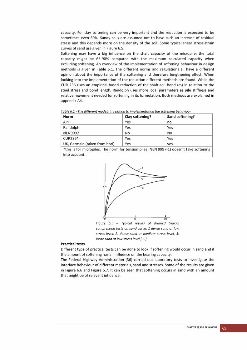
CHAPTER 6| SOIL BEHAVIOUR 69
capacity. For clay softening can be very important and the reduction is expected to be
sometimes even 50%. Sandy soils are assumed not to have such an increase of residual
stress and this depends more on the density of the soil. Some typical shear stress-strain
curves of sand are given in Figure 6.5.
Softening may have a big influence on the shaft capacity of the micropile: the total
capacity might be 65-90% compared with the maximum calculated capacity when
excluding softening. An overview of the implementation of softening behaviour in design
methods is given in Table 6.1. The different norms and regulations all have a different
opinion about the importance of the softening and therefore lengthening effect. When
looking into the implementation of the reduction different methods are found. While the
CUR 236 uses an empirical based reduction of the shaft-soil bond (αt) in relation to the
steel stress and bond length, Randolph uses more local parameters as pile stiffness and
relative movement needed for softening in its formulation. Both methods are explained in
appendix A4.
Table 6.1 - The different models in relation to implementation the softening behaviour
Norm Clay softening? Sand softening?
API Yes no
Randolph Yes Yes
NEN9997 No No
CUR236* Yes Yes
UK, Germain (taken from bbri) Yes yes
*this is for micropiles. The norm for tension piles (NEN 9997-1) doesn’t take softening
into account.
Figure 6.5 – Typical results of drained triaxial
compression tests on sand curve: 1 dense sand at low
stress level, 2: dense sand at medium stress level, 3:
loose sand at low stress level [35]
Practical tests
Different type of practical tests can be done to look if softening would occur in sand and if
the amount of softening has an influence on the bearing capacity.
The Federal Highway Administration [36] carried out laboratory tests to investigate the
interface behaviour of different materials, sand and stresses. Some of the results are given
in Figure 6.6 and Figure 6.7. It can be seen that softening occurs in sand with an amount
that might be of relevant influence.
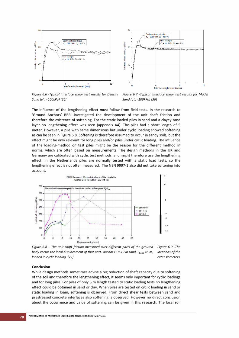
70 PERFORMANCE OF MICROPILES UNDER AXIAL TENSILE LOADING |MSc Thesis
Figure 6.6 -Typical interface shear test results for Density
Sand (σ’n ≈100kPa) [36]
Figure 6.7 -Typical interface shear test results for Model
Sand (σ’n ≈100kPa) [36]
The influence of the lengthening effect must follow from field tests. In the research to
‘Ground Anchors’ BBRI investigated the development of the unit shaft friction and
therefore the existence of softening. For the static loaded piles in sand and a clayey sand
layer no lengthening effect was seen (appendix A4). The piles had a short length of 5
meter. However, a pile with same dimensions but under cyclic loading showed softening
as can be seen in Figure 6.8. Softening is therefore assumed to occur in sandy soils, but the
effect might be only relevant for long piles and/or piles under cyclic loading. The influence
of the loading-method on test piles might be the reason for the different method in
norms, which are often based on measurements. The design methods in the UK and
Germany are calibrated with cyclic test methods, and might therefore use the lengthening
effect. In the Netherlands piles are normally tested with a static load tests, so the
lengthening effect is not often measured. The NEN 9997-1 also did not take softening into
account.
Figure 6.8 – The unit shaft friction measured over different parts of the grouted
body versus the local displacement of that part. Anchor E18-19 in sand, Lbond =5 m,
loaded in cyclic loading. [22]
Figure 6.9 -The
locations of the
extensiometers
Conclusion
While design methods sometimes advise a big reduction of shaft capacity due to softening
of the soil and therefore the lengthening effect, it seems only important for cyclic loadings
and for long piles. For piles of only 5 m length tested to static loading tests no lengthening
effect could be obtained in sand or clay. When piles are tested on cyclic loading in sand or
static loading in loam, softening is observed. From direct shear tests between sand and
prestressed concrete interfaces also softening is observed. However no direct conclusion
about the occurrence and value of softening can be given in this research. The local soil
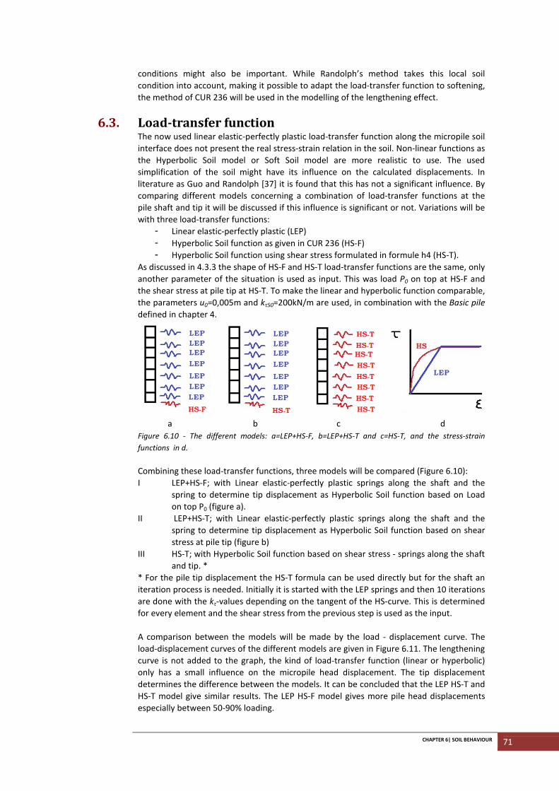
CHAPTER 6| SOIL BEHAVIOUR 71
conditions might also be important. While Randolph’s method takes this local soil
condition into account, making it possible to adapt the load-transfer function to softening,
the method of CUR 236 will be used in the modelling of the lengthening effect.
6.3. Load-transfer function The now used linear elastic-perfectly plastic load-transfer function along the micropile soil
interface does not present the real stress-strain relation in the soil. Non-linear functions as
the Hyperbolic Soil model or Soft Soil model are more realistic to use. The used
simplification of the soil might have its influence on the calculated displacements. In
literature as Guo and Randolph [37] it is found that this has not a significant influence. By
comparing different models concerning a combination of load-transfer functions at the
pile shaft and tip it will be discussed if this influence is significant or not. Variations will be
with three load-transfer functions:
- Linear elastic-perfectly plastic (LEP)
- Hyperbolic Soil function as given in CUR 236 (HS-F)
- Hyperbolic Soil function using shear stress formulated in formule h4 (HS-T).
As discussed in 4.3.3 the shape of HS-F and HS-T load-transfer functions are the same, only
another parameter of the situation is used as input. This was load P0 on top at HS-F and
the shear stress at pile tip at HS-T. To make the linear and hyperbolic function comparable,
the parameters u0=0,005m and kτ50=200kN/m are used, in combination with the Basic pile
defined in chapter 4.
a b c d
Figure 6.10 - The different models: a=LEP+HS-F, b=LEP+HS-T and c=HS-T, and the stress-strain
functions in d.
Combining these load-transfer functions, three models will be compared (Figure 6.10):
I LEP+HS-F; with Linear elastic-perfectly plastic springs along the shaft and the
spring to determine tip displacement as Hyperbolic Soil function based on Load
on top P0 (figure a).
II LEP+HS-T; with Linear elastic-perfectly plastic springs along the shaft and the
spring to determine tip displacement as Hyperbolic Soil function based on shear
stress at pile tip (figure b)
III HS-T; with Hyperbolic Soil function based on shear stress - springs along the shaft
and tip. *
* For the pile tip displacement the HS-T formula can be used directly but for the shaft an
iteration process is needed. Initially it is started with the LEP springs and then 10 iterations
are done with the kτ-values depending on the tangent of the HS-curve. This is determined
for every element and the shear stress from the previous step is used as the input.
A comparison between the models will be made by the load - displacement curve. The
load-displacement curves of the different models are given in Figure 6.11. The lengthening
curve is not added to the graph, the kind of load-transfer function (linear or hyperbolic)
only has a small influence on the micropile head displacement. The tip displacement
determines the difference between the models. It can be concluded that the LEP HS-T and
HS-T model give similar results. The LEP HS-F model gives more pile head displacements
especially between 50-90% loading.
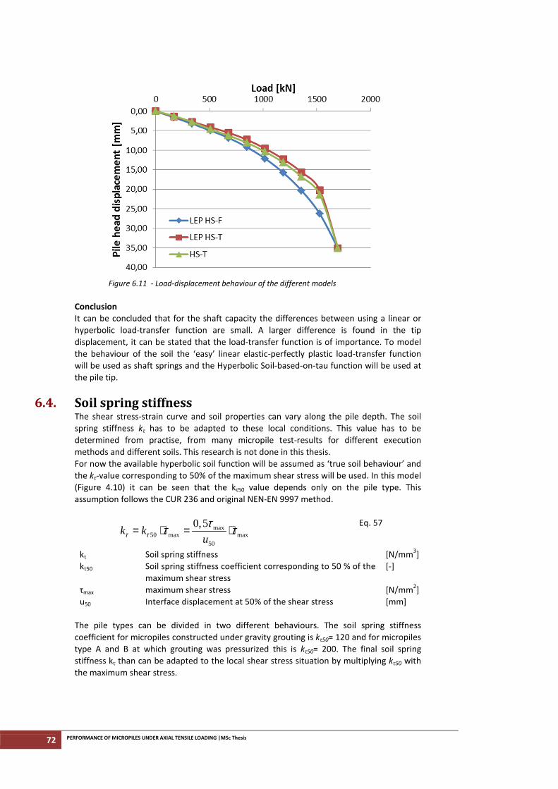
72 PERFORMANCE OF MICROPILES UNDER AXIAL TENSILE LOADING |MSc Thesis
Figure 6.11 - Load-displacement behaviour of the different models
Conclusion
It can be concluded that for the shaft capacity the differences between using a linear or
hyperbolic load-transfer function are small. A larger difference is found in the tip
displacement, it can be stated that the load-transfer function is of importance. To model
the behaviour of the soil the ‘easy’ linear elastic-perfectly plastic load-transfer function
will be used as shaft springs and the Hyperbolic Soil-based-on-tau function will be used at
the pile tip.
6.4. Soil spring stiffness The shear stress-strain curve and soil properties can vary along the pile depth. The soil
spring stiffness kτ has to be adapted to these local conditions. This value has to be
determined from practise, from many micropile test-results for different execution
methods and different soils. This research is not done in this thesis.
For now the available hyperbolic soil function will be assumed as ‘true soil behaviour’ and
the kτ-value corresponding to 50% of the maximum shear stress will be used. In this model
(Figure 4.10) it can be seen that the kτ50 value depends only on the pile type. This
assumption follows the CUR 236 and original NEN-EN 9997 method.
max
50 max max50
0,5k k
uτ τττ τ= ⋅ = ⋅
Eq. 57
kτ Soil spring stiffness [N/mm3]
kτ50 Soil spring stiffness coefficient corresponding to 50 % of the
maximum shear stress
[-]
τmax maximum shear stress [N/mm2]
u50 Interface displacement at 50% of the shear stress [mm]
The pile types can be divided in two different behaviours. The soil spring stiffness
coefficient for micropiles constructed under gravity grouting is kτ50= 120 and for micropiles
type A and B at which grouting was pressurized this is kτ50= 200. The final soil spring
stiffness kτ than can be adapted to the local shear stress situation by multiplying kτ50 with
the maximum shear stress.
CHAPTER 6| SOIL BEHAVIOUR 73
6.5. Non-homogeneous soil The analytical model to determine the displacement given in chapter 4 is for a
homogeneous soil: all load-transfer curves are equal and the transition point between the
plastic and elastic interaction between micropile and soil is determined by an analytical
calculation. Normally soils and its stresses are not homogeneous, so this has to be
implemented in the model. In literature it is found that this can be implemented by a non-
homogeneity factor n (Gou and Randolph [37]), using complex matrix calculations for
every depth (Liu et al [38]), using ratios for each soil layer (Ai and Yue [39]) or using
numerical methods (Van Dalen [20] or Chen and Yao [41]).
When modelling non-homogeneous soils it is important that for each layer the properties
of the soil can be varied. These variations will be in the maximum shear stress (cone
resistance qc and αt) and the shape of the stress-strain curve (kτ50). It is possible to
implement non-homogeneous soils using the analytical method. The pile is therefore
discretised in elements in series.
The calculation will then be started as normal with the top element (No.1) of the pile. The
axial force in the top of this element is load P0. The shear stress that can be developed is
the maximum shear stress (in case of a plastic micropile soil interaction) or a lower value
(in case of elastic interaction). Using Eq. 16 and Eq. 12 the axial force at the base of the
each element will be calculated, suggesting plastic respectively elastic interaction at the
pile shaft. The shear stress may not be more than the maximum, therefore the axial force
in the pile may not decrease more than determined by the plastic interaction-calculation:
the maximum normal force in the pile following the elastic and plastic calculation will be
the actual normal force in the base of the element (Eq. 58). For the second element the
calculation has to be done again using the axial force governing on top of this element.
This axial force follows from the base of element No. 1. To determine the elastic
interaction the pile length has to be adapted to the calculation, because the new fictive
pile is shorter namely Lb minus the height of element No.1. The calculation has to be done
for each element to pile tip. Using this method it is possible to use different soil-
parameters in this calculation.
0 max( )pl gN z P D zπ τ= − ⋅ ⋅ ⋅ for z<zl
0
sinh( ) ( )
sinh
bl
z
el gel
b l
L zN
N z z DL z
λτ π
λ
− = ⋅ =
−
∫ for z>zl
( ) max[ ( ), ( )]pl elN z N z N z=
is Eq. 16
is Eq. 12
Eq. 58
When using this method in homogeneous soil the same transition point will be found as
using the formulation given in Eq. 19. For non-homogeneous soil it is possible that there
are more transition points. In Figure 6.12 this is shown for a fictive soil with layering; the
maximum possible shear stress τmax and the shear stress that will be developed τ(z) are
given.
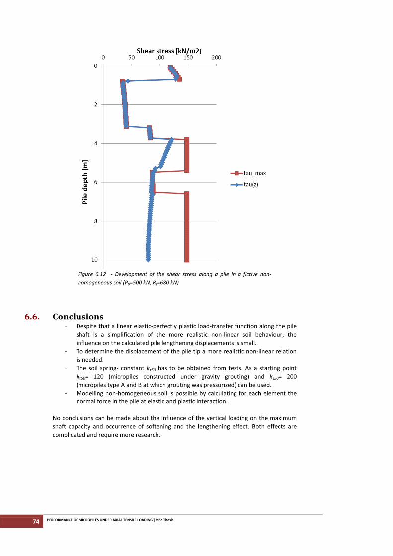
74 PERFORMANCE OF MICROPILES UNDER AXIAL TENSILE LOADING |MSc Thesis
Figure 6.12 - Development of the shear stress along a pile in a fictive non-
homogeneous soil.(P0=500 kN, Rt=680 kN)
6.6. Conclusions - Despite that a linear elastic-perfectly plastic load-transfer function along the pile
shaft is a simplification of the more realistic non-linear soil behaviour, the
influence on the calculated pile lengthening displacements is small.
- To determine the displacement of the pile tip a more realistic non-linear relation
is needed.
- The soil spring- constant kτ50 has to be obtained from tests. As a starting point
kτ50= 120 (micropiles constructed under gravity grouting) and kτ50= 200
(micropiles type A and B at which grouting was pressurized) can be used.
- Modelling non-homogeneous soil is possible by calculating for each element the
normal force in the pile at elastic and plastic interaction.
No conclusions can be made about the influence of the vertical loading on the maximum
shaft capacity and occurrence of softening and the lengthening effect. Both effects are
complicated and require more research.
CHAPTER 7| FINAL MODEL: RFM 75
7 FINAL MODEL: RFM
Now the final model can be constructed and validated since the basic model is explained
and research is done into structural and soil behaviour. A short description and the
possibilities of the model called “RFM” will be explained first. Validation will be done by
using a case and the comparison with other models. Then the performance of a micropile
loaded in tension will be discussed. Parameters as length and steel diameter have a
different influence on the pile performance, this will be discussed as well. Finally the
extensive calculation method from the model is simplified to a formulation based on the
original performance calculation method of the CUR 236.
7.1. Revised FOREVER model Combining the calculation method using load-transfer functions along the shaft explained
in chapter 4 and all researches, a final model called “Revised FOREVER model” (RFM) can
be presented. This name is chosen because the model in this study is based on research
from the French National Project on Micropiles entitled Fondations Renforcées
Verticalement which was a big research project to understand the performance of
micropile(groups). The project used a linear elastic-perfectly plastic model as shaft friction
interface mobilisation to simulate the real development of the pile capacity and pile head
displacement. Officially, the original derivation of the analytical calculation method is done
by Mr Scott, but the FOREVER program is more famous and therefore this method is given
this name.
The model consists of three parts: the determination of the maximum capacity, the
displacement during loading and the micropile’s performance. All formulas and a full
description of the model are given in appendix A5. The modelling is done in Excel. An
explanation of the sheet is given in appendix A6. In this Excel document the full calculation
is modelled from soil investigation (CPT), via the calculation of the bearing capacity and
displacements, to the calculation of the micropile’s performance is modelled. Information
about the calculation can be found in the Excel sheet and appendix A6. In this paragraph a
short description of the model and its possibilities are given.
The RFM combines the current method to determine the capacity of a pile conform
NEN 9997-1 and CUR 236 with the calculation of the pile head displacement to obtain the
micropile’s performance. In the model the pile is divided in elements and the adjacent soil
is modelled by load-transfer functions connected to the elements. For each element the
local equilibrium is valid: the shaft friction created determines the capacity of the element.
The shear stresses are related to the displacement and the elements are connected, with
as result that the shear stress of each element is related to the shear stress of the other
76 PERFORMANCE OF MICROPILES UNDER AXIAL TENSILE LOADING |MSc Thesis
elements. The model is load-orientated and uses a linear elastic-perfectly plastic relation
as load-transfer curve and can therefore be solved analytical.
Because the pile is discretised in elements it is possible to implement various situations in
the model. The size of the elements can depend on the soil layering following from the
CPT. The soil conditions can as well vary with depth following this CPT. The pile-type and
dimensions of the pile are taken into account as well, including a possible variation in
grout diameter. The axial stiffness of the micropile can differ over the pile length, to
implement grout-cracking. Furthermore the effects determining the maximum shear stress
(group effect and tensile loading) can be implemented as well. The output of the model is
not only the calculated maximum bearing capacity, the expected displacement under a
certain loading and the micropile’s performance but gives as well insight into the load-
transfer from the pile to the soil.
Only a couple of parameters are extra needed for the displacement calculation compared
with the parameters needed to calculate the pile capacity using the current methods.
These parameters are: Young’s moduli of steel and grout, the diameter of steel and the
pile type or soil stiffness coefficient kτ50. Due to the implementation of the grout cracking
also the tension strain of grout is added.
A limitation of this Revised FOREVER model is that the displacement and performance can
only be determined for tension piles. This is because at compression the pile tip develops
capacity as well. The stress-strain relation of the pile tip is different from the now assumed
stress-strain relation.. The important boundary condition that the force at pile tip is zero is
not valid any more, implementation of compression loads would therefore be difficult and
iterations are needed. However, due to the relatively good compression capacity of grout
the pile is expected to behave more rigid. A second limitation is that softening is not
implemented. It is possible to implement softening but then iterations are needed in the
calculation.
The model is designed for micropiles but can be used for other piles as well. The relation
between the pile and soil by the stiffness coefficient of the soil kτ50 has to be adapted in
that case to the right pile type and execution method. Another difference would be that
the calculation of the distance between cracks and crack width at grout-cracking is made
using the normal rules for reinforcement and the results of a TITAN pull-out test. This
formulation has to be adapted when other reinforcements are used to obtain a realistic
cracking behaviour.
7.2. Validation of the model To see if the model gives a good representation of the real micropile behaviour the model
has to be validated. Most satisfying is the check with results from field work. Due to
differences between the expected and real parameters as dimension and soil strength
there will be a slight difference between the results. In section 7.2.1 the model is
compared with test results of two 11,1 m long piles. Another validation method is the
verification with other (validated) models. The model will be compared with two
numerical displacement controlled models.
7.2.1. Case A set of test piles will be used to validate the model. These GEWI micropiles are 11,1 m
long, have a reinforcement diameter of 50 mm and an assumed grout diameter of
200 mm. The soil had an average strength of 12,5 MPa. The piles were tested to obtain the
micropile’s axial spring stiffness (suitability test). The piles are therefore tested for
relatively low loads, the testing load was 770 kN in comparison while the bearing capacity
of the pile due to the soil properties would be 1700 kN. The spring stiffness calculation
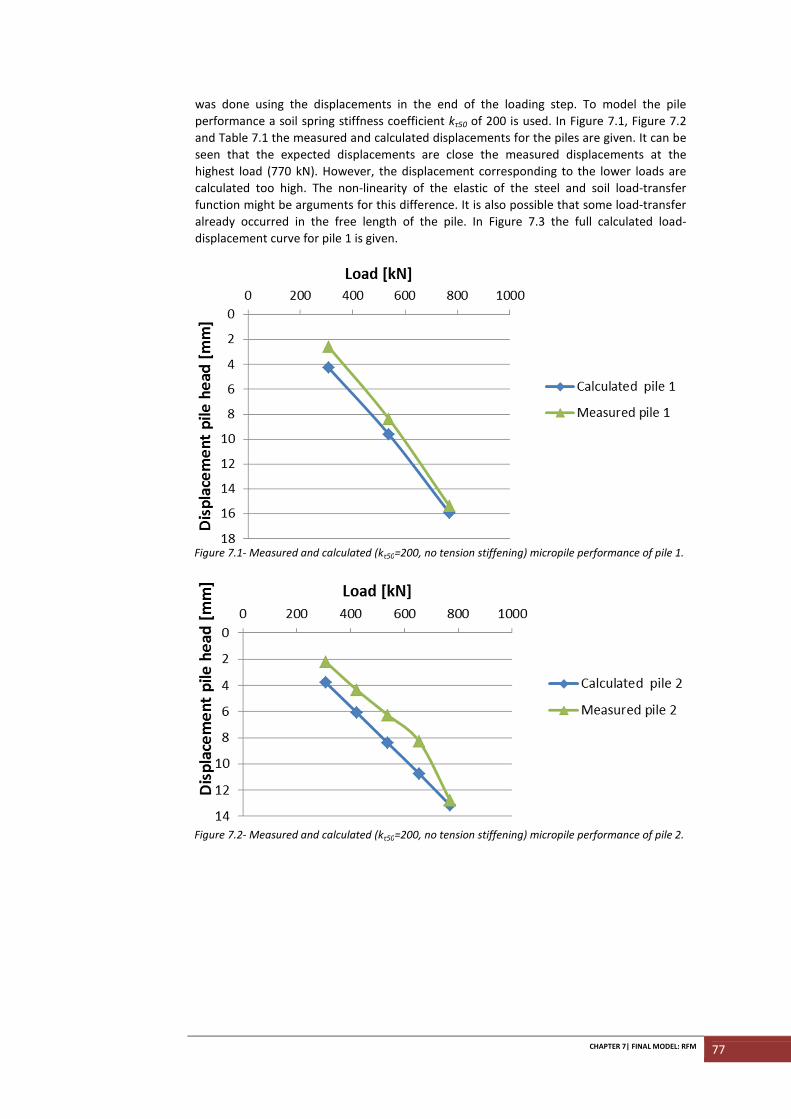
CHAPTER 7| FINAL MODEL: RFM 77
was done using the displacements in the end of the loading step. To model the pile
performance a soil spring stiffness coefficient kτ50 of 200 is used. In Figure 7.1, Figure 7.2
and Table 7.1 the measured and calculated displacements for the piles are given. It can be
seen that the expected displacements are close the measured displacements at the
highest load (770 kN). However, the displacement corresponding to the lower loads are
calculated too high. The non-linearity of the elastic of the steel and soil load-transfer
function might be arguments for this difference. It is also possible that some load-transfer
already occurred in the free length of the pile. In Figure 7.3 the full calculated load-
displacement curve for pile 1 is given.
Figure 7.1- Measured and calculated (kτ50=200, no tension stiffening) micropile performance of pile 1.
Figure 7.2- Measured and calculated (kτ50=200, no tension stiffening) micropile performance of pile 2.
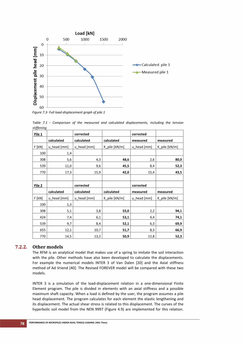
78 PERFORMANCE OF MICROPILES UNDER AXIAL TENSILE LOADING |MSc Thesis
Figure 7.3- Full load-displacement graph of pile 1
Table 7.1 - Comparison of the measured and calculated displacements, including the tension
stiffening
Pile 1 corrected corrected
calculated calculated calculated measured measured
F [kN] u_head [mm] u_head [mm] K_pile [kN/m] u_head [mm] K_pile [kN/m]
100 1,4
308 5,6 4,3 48,6 2,6 80,0
539 11,0 9,6 45,5 8,4 52,3
770 17,3 15,9 42,0 15,4 43,5
Pile 2 corrected corrected
calculated calculated calculated measured measured
F [kN] u_head [mm] u_head [mm] K_pile [kN/m] u_head [mm] K_pile [kN/m]
100 1,3
308 5,1 3,8 55,0 2,2 94,1
424 7,4 6,1 53,1 4,4 74,1
539 9,7 8,4 52,1 6,3 69,9
655 12,1 10,7 51,7 8,3 66,9
770 14,5 13,2 50,9 12,8 52,3
7.2.2. Other models The RFM is an analytical model that makes use of a spring to imitate the soil interaction
with the pile. Other methods have also been developed to calculate the displacements.
For example the numerical models INTER 3 of Van Dalen [20] and the Axial stiffness
method of Ad Vriend [40]. The Revised FOREVER model will be compared with these two
models.
INTER 3 is a simulation of the load-displacement relation in a one-dimensional Finite
Element program. The pile is divided in elements with an axial stiffness and a possible
maximum shaft capacity. When a load is defined by the user, the program assumes a pile
head displacement. The program calculates for each element the elastic lengthening and
its displacement. The actual shear stress is related to this displacement. The curves of the
hyperbolic soil model from the NEN 9997 (Figure 4.9) are implemented for this relation.
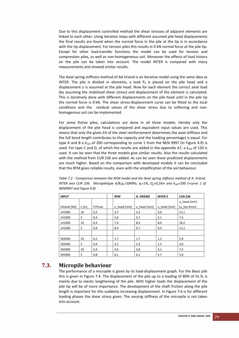
CHAPTER 7| FINAL MODEL: RFM 79
Due to this displacement controlled method the shear stresses of adjacent elements are
linked to each other. Using iteration steps with different assumed pile head displacements
the final results are found when the normal force in the pile at the tip is in accordance
with the tip displacement. For tension piles this results in 0 kN normal force at the pile tip.
Except for other load-transfer functions the model can be used for tension and
compression piles, as well as non-homogeneous soil. Moreover the effects of load history
on the pile can be taken into account. The model INTER is compared with many
measurements and showed similar results.
The Axial spring stiffness method of Ad Vriend is an iterative model using the same idea as
INTER. The pile is divided in elements, a load P0 is placed on the pile head and a
displacement u is assumed at the pile head. Now for each element the correct axial load
(by assuming the mobilised shear stress) and displacement of the element is calculated.
This is iteratively done with different displacements on the pile head until in the pile tip
the normal force is 0 kN. The shear stress-displacement curve can be fitted to the local
conditions and the residual values of the shear stress due to softening and non-
homogenous soil can be implemented.
For some fictive piles, calculations are done in all three models. Hereby only the
displacement of the pile head is compared and equivalent input values are used. This
means that only the given EA of the steel reinforcement determines the axial stiffness and
the full bond length contributes to the capacity and the load(ing percentage) is equal. For
type A and B a kτ50 of 200 corresponding to curve 1 from the NEN 9997 (in Figure 4.9) is
used. For type C and D, of which the results are added in the appendix A7, a kτ50 of 120 is
used. It can be seen that the three models give similar results. Also the results calculated
with the method from CUR 236 are added. As can be seen these predicted displacements
are much higher. Based on the comparison with developed models it can be concluded
that the RFM gives reliable results, even with the simplification of the soil behaviour.
Table 7.2 - Comparison between the RFM model and the Axial spring stiffness method of A. Vriend,
INTER and CUR 236. Micropiletype A/B,qc=20MPa, αt=1%, Dg=0,16m and kτ50=200 (=curve 1 of
NEN9997 and Figure 4.9)
INPUT RFM A. VRIEND INTER 3 CUR 236
EAsteel [kN] L [m] F/Fmax u_head [mm] u_head [mm] u_head [mm]
u_head [mm]
(u_tip=4mm)
141000 10 0,2 3,7 3,3 3,0 11,1
141000 5 0,4 3,6 3,7 3,1 7,5
141000 10 0,4 7,9 8,4 8,0 18,2
141000 5 0,8 8,9 9,7 9,3 11,1
565000 10 0,2 1,7 1,7 1,2 5,8
565000 5 0,4 2,2 2,3 1,5 4,9
565000 10 0,4 3,6 3,8 3,1 7,5
565000 5 0,8 6,1 6,1 5.7 5,8
7.3. Micropile behaviour The performance of a micropile is given by its load-displacement graph. For the Basic pile
this is given in Figure 7.4. The displacement of the pile up to a loading of 80% of its Rt is
mainly due to elastic lengthening of the pile. With higher loads the displacement of the
pile tip will be of more importance. The development of the shaft friction along the pile
length is important for this suddenly increasing displacement. In Figure 7.6 is for different
loading phases the shear stress given. The varying stiffness of the micropile is not taken
into account.
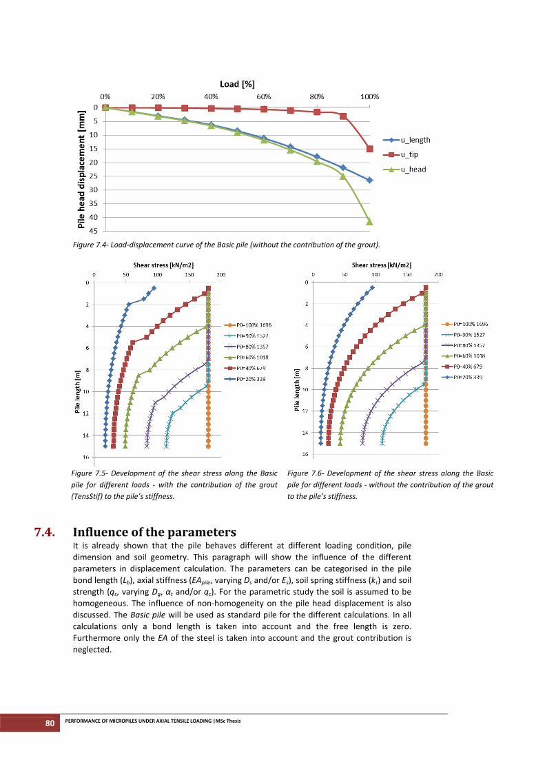
80 PERFORMANCE OF MICROPILES UNDER AXIAL TENSILE LOADING |MSc Thesis
Figure 7.4- Load-displacement curve of the Basic pile (without the contribution of the grout).
Figure 7.5- Development of the shear stress along the Basic
pile for different loads - with the contribution of the grout
(TensStif) to the pile’s stiffness.
Figure 7.6- Development of the shear stress along the Basic
pile for different loads - without the contribution of the grout
to the pile’s stiffness.
7.4. Influence of the parameters It is already shown that the pile behaves different at different loading condition, pile
dimension and soil geometry. This paragraph will show the influence of the different
parameters in displacement calculation. The parameters can be categorised in the pile
bond length (Lb), axial stiffness (EApile, varying Ds and/or Es), soil spring stiffness (kτ) and soil
strength (qs, varying Dg, αt and/or qc). For the parametric study the soil is assumed to be
homogeneous. The influence of non-homogeneity on the pile head displacement is also
discussed. The Basic pile will be used as standard pile for the different calculations. In all
calculations only a bond length is taken into account and the free length is zero.
Furthermore only the EA of the steel is taken into account and the grout contribution is
neglected.
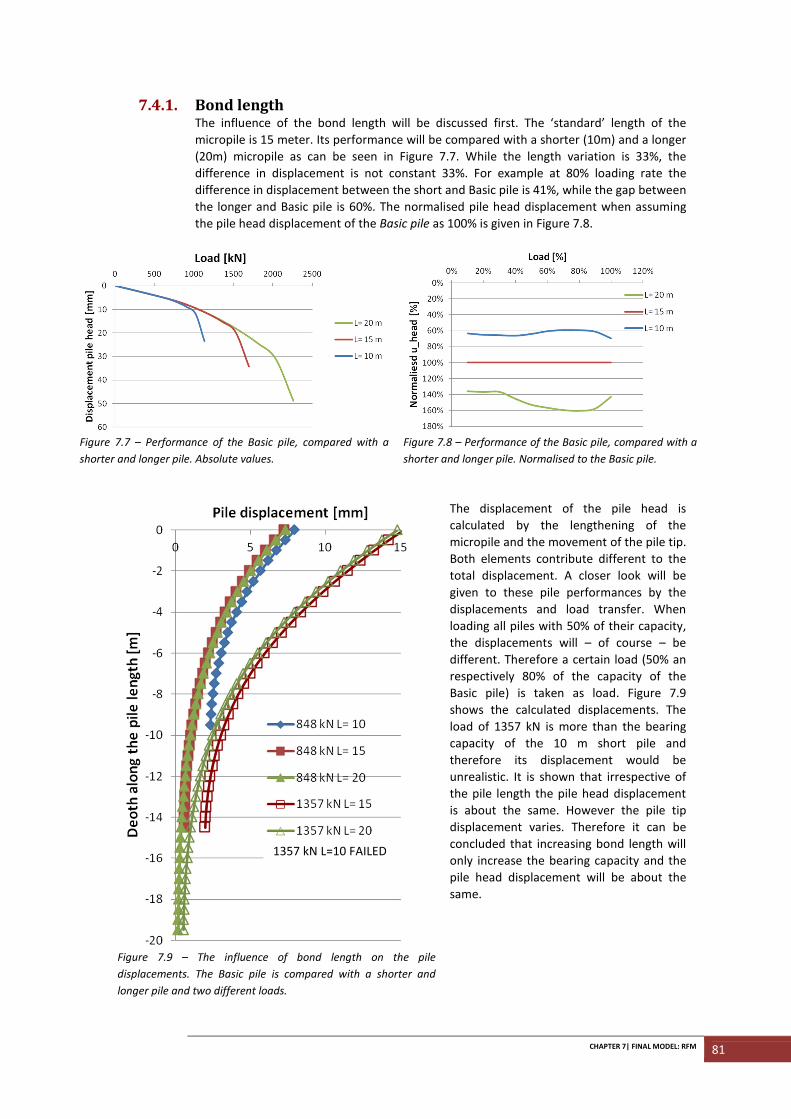
CHAPTER 7| FINAL MODEL: RFM 81
7.4.1. Bond length The influence of the bond length will be discussed first. The ‘standard’ length of the
micropile is 15 meter. Its performance will be compared with a shorter (10m) and a longer
(20m) micropile as can be seen in Figure 7.7. While the length variation is 33%, the
difference in displacement is not constant 33%. For example at 80% loading rate the
difference in displacement between the short and Basic pile is 41%, while the gap between
the longer and Basic pile is 60%. The normalised pile head displacement when assuming
the pile head displacement of the Basic pile as 100% is given in Figure 7.8.
Figure 7.7 – Performance of the Basic pile, compared with a
shorter and longer pile. Absolute values.
Figure 7.8 – Performance of the Basic pile, compared with a
shorter and longer pile. Normalised to the Basic pile.
The displacement of the pile head is
calculated by the lengthening of the
micropile and the movement of the pile tip.
Both elements contribute different to the
total displacement. A closer look will be
given to these pile performances by the
displacements and load transfer. When
loading all piles with 50% of their capacity,
the displacements will – of course – be
different. Therefore a certain load (50% an
respectively 80% of the capacity of the
Basic pile) is taken as load. Figure 7.9
shows the calculated displacements. The
load of 1357 kN is more than the bearing
capacity of the 10 m short pile and
therefore its displacement would be
unrealistic. It is shown that irrespective of
the pile length the pile head displacement
is about the same. However the pile tip
displacement varies. Therefore it can be
concluded that increasing bond length will
only increase the bearing capacity and the
pile head displacement will be about the
same.
Figure 7.9 – The influence of bond length on the pile
displacements. The Basic pile is compared with a shorter and
longer pile and two different loads.
1357 kN L=10 FAILED
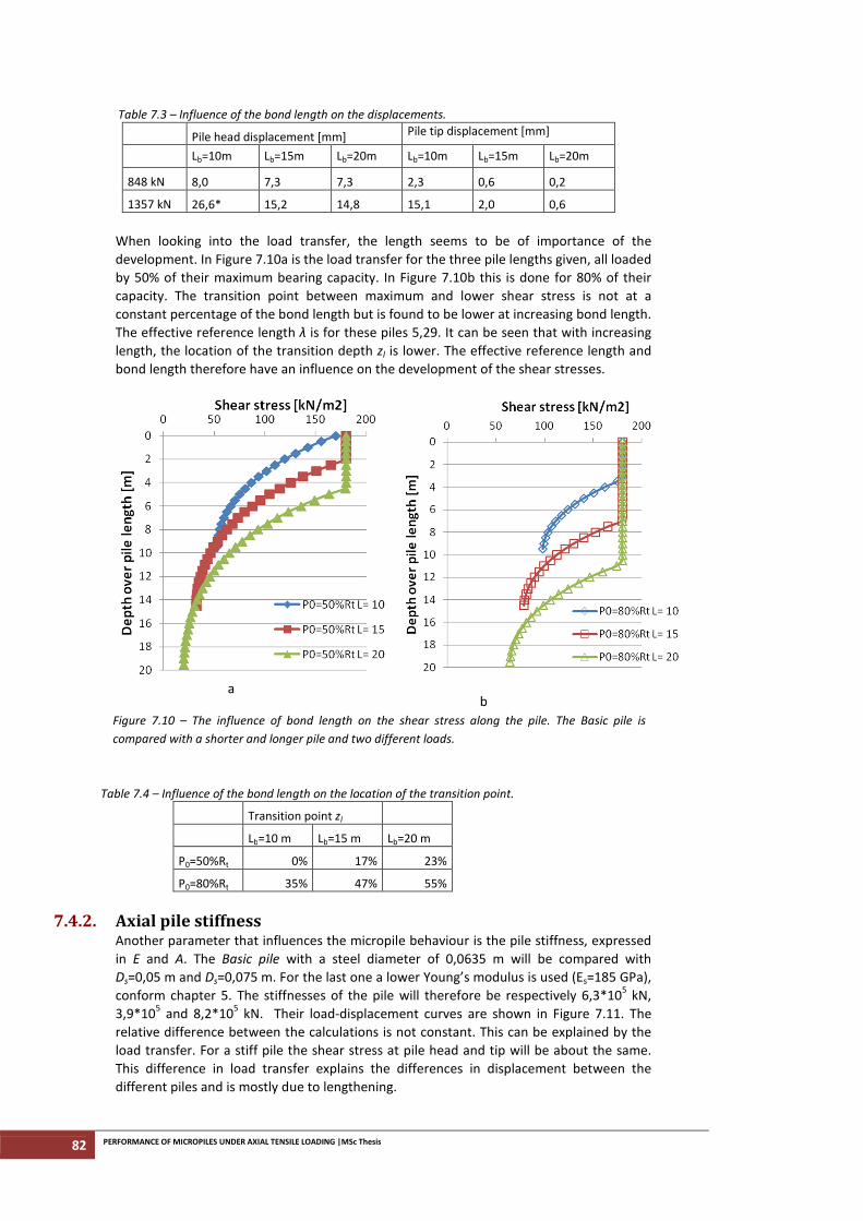
82 PERFORMANCE OF MICROPILES UNDER AXIAL TENSILE LOADING |MSc Thesis
Table 7.3 – Influence of the bond length on the displacements.
Pile head displacement [mm] Pile tip displacement [mm]
Lb=10m Lb=15m Lb=20m Lb=10m Lb=15m Lb=20m
848 kN 8,0 7,3 7,3 2,3 0,6 0,2
1357 kN 26,6* 15,2 14,8 15,1 2,0 0,6
When looking into the load transfer, the length seems to be of importance of the
development. In Figure 7.10a is the load transfer for the three pile lengths given, all loaded
by 50% of their maximum bearing capacity. In Figure 7.10b this is done for 80% of their
capacity. The transition point between maximum and lower shear stress is not at a
constant percentage of the bond length but is found to be lower at increasing bond length.
The effective reference length λ is for these piles 5,29. It can be seen that with increasing
length, the location of the transition depth zl is lower. The effective reference length and
bond length therefore have an influence on the development of the shear stresses.
a
b
Figure 7.10 – The influence of bond length on the shear stress along the pile. The Basic pile is
compared with a shorter and longer pile and two different loads.
Table 7.4 – Influence of the bond length on the location of the transition point.
Transition point zl
Lb=10 m Lb=15 m Lb=20 m
P0=50%Rt 0% 17% 23%
P0=80%Rt 35% 47% 55%
7.4.2. Axial pile stiffness Another parameter that influences the micropile behaviour is the pile stiffness, expressed
in E and A. The Basic pile with a steel diameter of 0,0635 m will be compared with
Ds=0,05 m and Ds=0,075 m. For the last one a lower Young’s modulus is used (Es=185 GPa),
conform chapter 5. The stiffnesses of the pile will therefore be respectively 6,3*105 kN,
3,9*105 and 8,2*10
5 kN. Their load-displacement curves are shown in Figure 7.11. The
relative difference between the calculations is not constant. This can be explained by the
load transfer. For a stiff pile the shear stress at pile head and tip will be about the same.
This difference in load transfer explains the differences in displacement between the
different piles and is mostly due to lengthening.
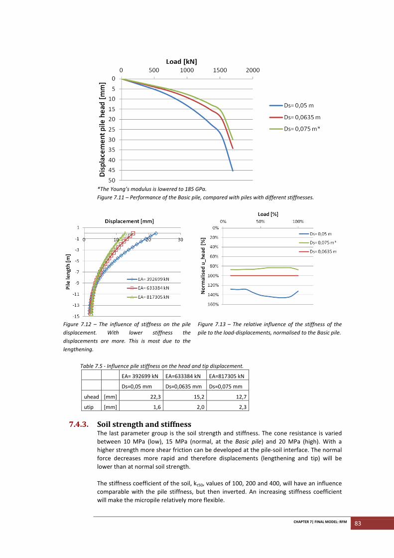
CHAPTER 7| FINAL MODEL: RFM 83
*The Young’s modulus is lowered to 185 GPa.
Figure 7.11 – Performance of the Basic pile, compared with piles with different stiffnesses.
Figure 7.12 – The influence of stiffness on the pile
displacement. With lower stiffness the
displacements are more. This is most due to the
lengthening.
Figure 7.13 – The relative influence of the stiffness of the
pile to the load-displacements, normalised to the Basic pile.
Table 7.5 - Influence pile stiffness on the head and tip displacement.
EA= 392699 kN EA=633384 kN EA=817305 kN
Ds=0,05 mm Ds=0,0635 mm Ds=0,075 mm
uhead [mm] 22,3 15,2 12,7
utip [mm] 1,6 2,0 2,3
7.4.3. Soil strength and stiffness The last parameter group is the soil strength and stiffness. The cone resistance is varied
between 10 MPa (low), 15 MPa (normal, at the Basic pile) and 20 MPa (high). With a
higher strength more shear friction can be developed at the pile-soil interface. The normal
force decreases more rapid and therefore displacements (lengthening and tip) will be
lower than at normal soil strength.
The stiffness coefficient of the soil, kτ50, values of 100, 200 and 400, will have an influence
comparable with the pile stiffness, but then inverted. An increasing stiffness coefficient
will make the micropile relatively more flexible.
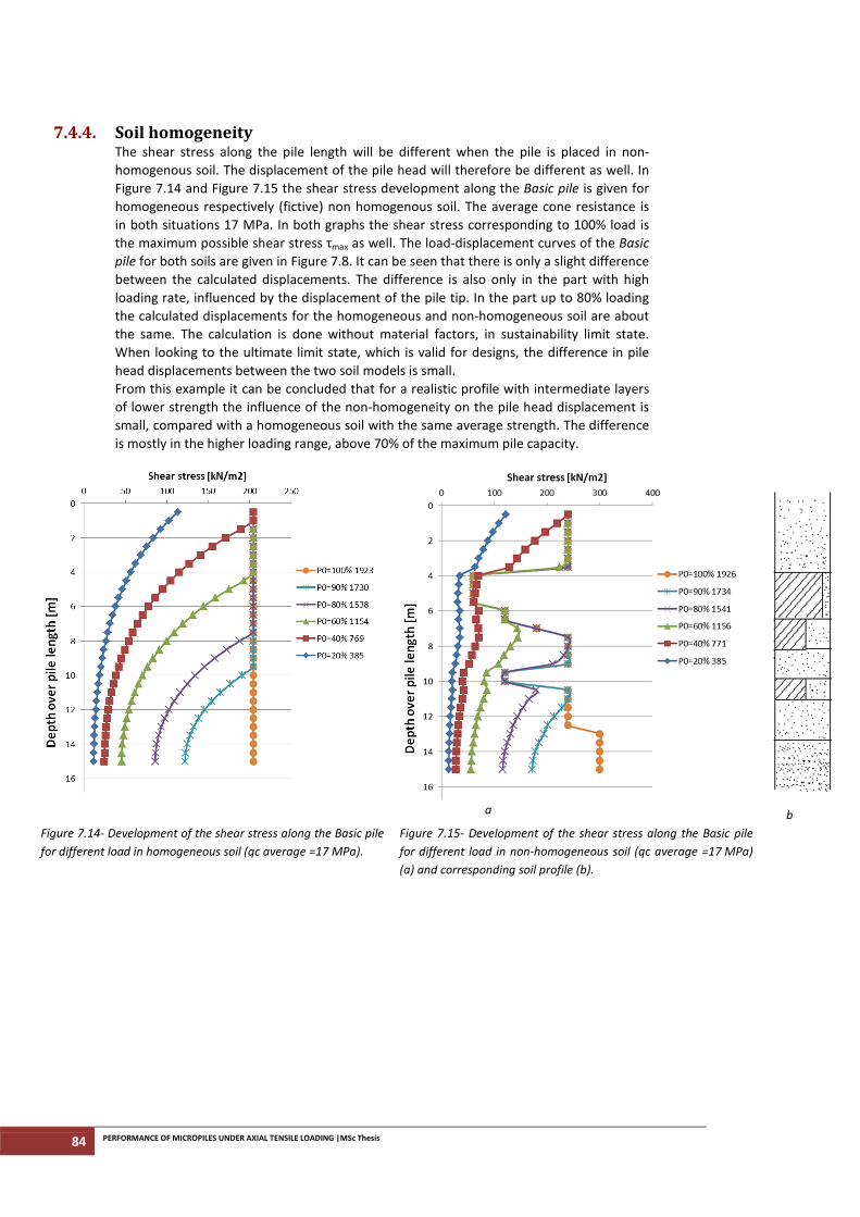
84 PERFORMANCE OF MICROPILES UNDER AXIAL TENSILE LOADING |MSc Thesis
7.4.4. Soil homogeneity The shear stress along the pile length will be different when the pile is placed in non-
homogenous soil. The displacement of the pile head will therefore be different as well. In
Figure 7.14 and Figure 7.15 the shear stress development along the Basic pile is given for
homogeneous respectively (fictive) non homogenous soil. The average cone resistance is
in both situations 17 MPa. In both graphs the shear stress corresponding to 100% load is
the maximum possible shear stress τmax as well. The load-displacement curves of the Basic
pile for both soils are given in Figure 7.8. It can be seen that there is only a slight difference
between the calculated displacements. The difference is also only in the part with high
loading rate, influenced by the displacement of the pile tip. In the part up to 80% loading
the calculated displacements for the homogeneous and non-homogeneous soil are about
the same. The calculation is done without material factors, in sustainability limit state.
When looking to the ultimate limit state, which is valid for designs, the difference in pile
head displacements between the two soil models is small.
From this example it can be concluded that for a realistic profile with intermediate layers
of lower strength the influence of the non-homogeneity on the pile head displacement is
small, compared with a homogeneous soil with the same average strength. The difference
is mostly in the higher loading range, above 70% of the maximum pile capacity.
a
b
Figure 7.14- Development of the shear stress along the Basic pile
for different load in homogeneous soil (qc average =17 MPa).
Figure 7.15- Development of the shear stress along the Basic pile
for different load in non-homogeneous soil (qc average =17 MPa)
(a) and corresponding soil profile (b).
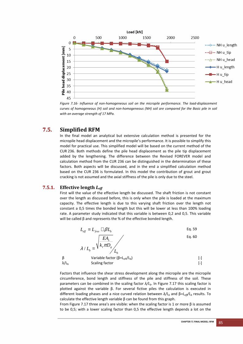
CHAPTER 7| FINAL MODEL: RFM 85
Figure 7.16- Influence of non-homogeneous soil on the micropile performance. The load-displacement
curves of homogeneous (H) soil and non-homogeneous (NH) soil are compared for the Basic pile in soil
with an average strength of 17 MPa.
7.5. Simplified RFM In the final model an analytical but extensive calculation method is presented for the
micropile head displacement and the micropile’s performance. It is possible to simplify this
model for practical use. This simplified model will be based on the current method of the
CUR 236. Both methods define the pile head displacement as the pile tip displacement
added by the lengthening. The difference between the Revised FOREVER model and
calculation method from the CUR 236 can be distinguished in the determination of these
factors. Both aspects will be discussed, and in the end a simplified calculation method
based on the CUR 236 is formulated. In this model the contribution of grout and grout
cracking is not assumed and the axial stiffness of the pile is only due to the steel.
7.5.1. Effective length Leff First will the value of the effective length be discussed. The shaft friction is not constant
over the length as discussed before, this is only when the pile is loaded at the maximum
capacity. The effective length is due to this varying shaft friction over the length not
constant a 0,5 times the bonded length but this will be lower at less than 100% loading
rate. A parameter study indicated that this variable is between 0,2 and 0,5. This variable
will be called β and represents the % of the effective bonded length.
eff free bL L Lβ= + Eq. 59
/
s
gb
b
EA
k DL L
τπλ =
Eq. 60
β Variable factor (β=Leff/Lb) [-]
λ/Lb Scaling factor [-]
Factors that influence the shear stress development along the micropile are the micropile
circumference, bond length and stiffness of the pile and stiffness of the soil. These
parameters can be combined in the scaling factor λ/Lb. In Figure 7.17 this scaling factor is
plotted against the variable β. For several fictive piles the calculation is executed in
different loading phases and a nice curved relation between λ/Lb and β=Leff/Lb results. To
calculate the effective length variable β can be found from this graph.
From Figure 7.17 three area’s are visible: when the scaling factor is 1 or more β is assumed
to be 0,5; with a lower scaling factor than 0,5 the effective length depends a lot on the
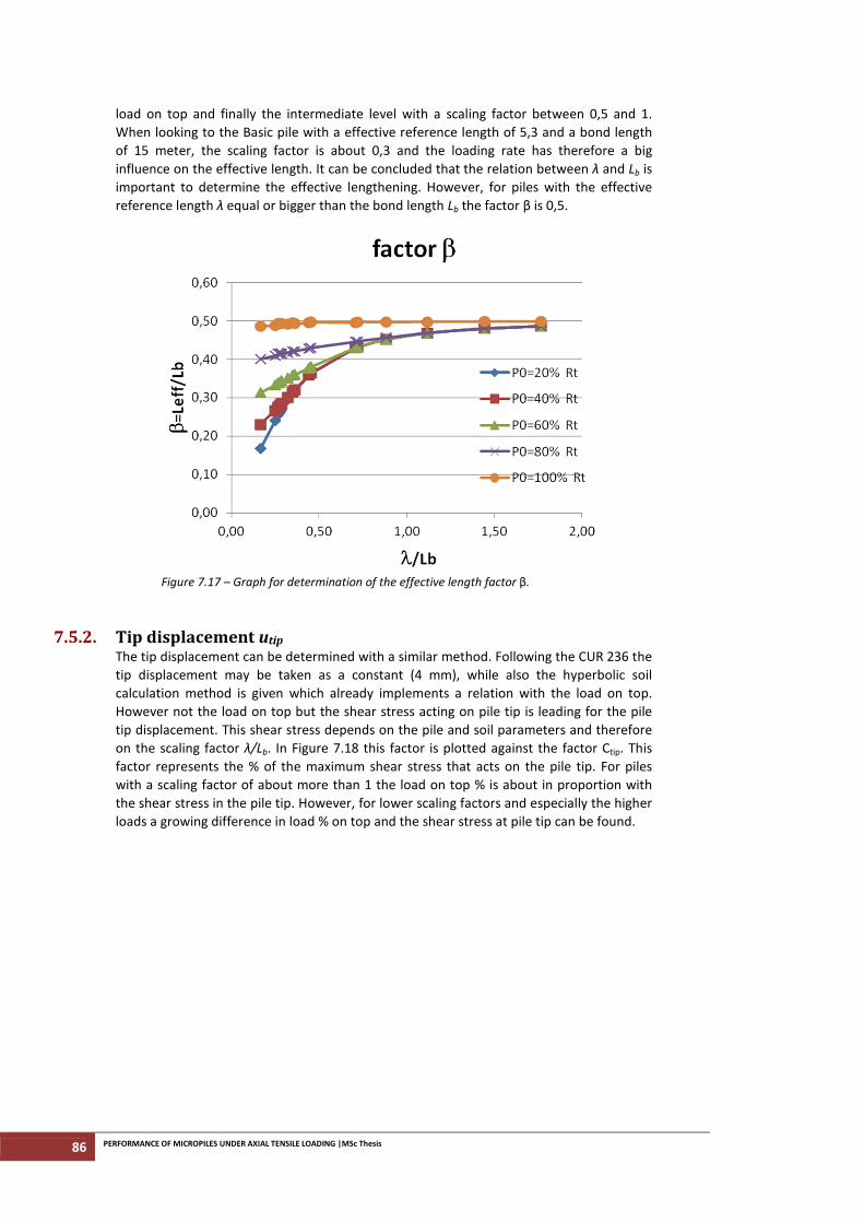
86 PERFORMANCE OF MICROPILES UNDER AXIAL TENSILE LOADING |MSc Thesis
load on top and finally the intermediate level with a scaling factor between 0,5 and 1.
When looking to the Basic pile with a effective reference length of 5,3 and a bond length
of 15 meter, the scaling factor is about 0,3 and the loading rate has therefore a big
influence on the effective length. It can be concluded that the relation between λ and Lb is
important to determine the effective lengthening. However, for piles with the effective
reference length λ equal or bigger than the bond length Lb the factor β is 0,5.
Figure 7.17 – Graph for determination of the effective length factor β.
7.5.2. Tip displacement utip The tip displacement can be determined with a similar method. Following the CUR 236 the
tip displacement may be taken as a constant (4 mm), while also the hyperbolic soil
calculation method is given which already implements a relation with the load on top.
However not the load on top but the shear stress acting on pile tip is leading for the pile
tip displacement. This shear stress depends on the pile and soil parameters and therefore
on the scaling factor λ/Lb. In Figure 7.18 this factor is plotted against the factor Ctip. This
factor represents the % of the maximum shear stress that acts on the pile tip. For piles
with a scaling factor of about more than 1 the load on top % is about in proportion with
the shear stress in the pile tip. However, for lower scaling factors and especially the higher
loads a growing difference in load % on top and the shear stress at pile tip can be found.
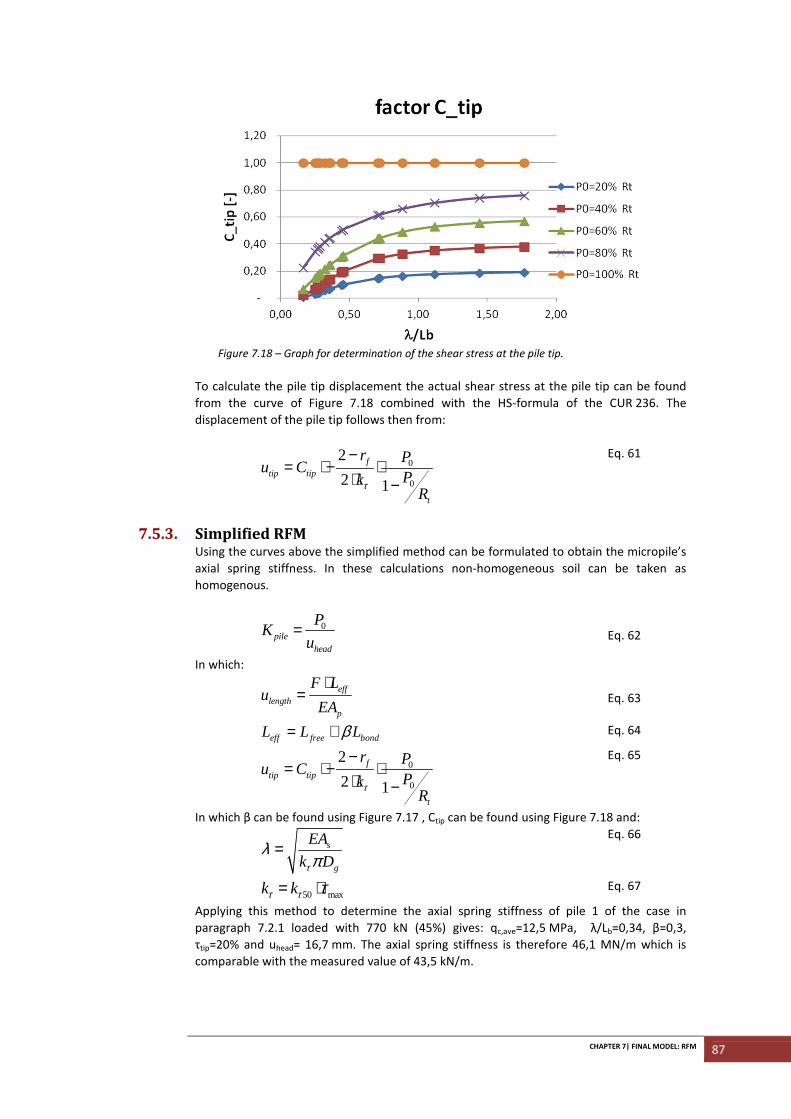
CHAPTER 7| FINAL MODEL: RFM 87
Figure 7.18 – Graph for determination of the shear stress at the pile tip.
To calculate the pile tip displacement the actual shear stress at the pile tip can be found
from the curve of Figure 7.18 combined with the HS-formula of the CUR 236. The
displacement of the pile tip follows then from:
0
0
2
2 1
ftip tip
t
r Pu C
PkR
τ
−= ⋅ − ⋅
⋅ −
Eq. 61
7.5.3. Simplified RFM Using the curves above the simplified method can be formulated to obtain the micropile’s
axial spring stiffness. In these calculations non-homogeneous soil can be taken as
homogenous.
0
pilehead
PK
u=
Eq. 62
In which:
eff
lengthp
F Lu
EA
⋅=
Eq. 63
eff free bondL L Lβ= + Eq. 64
0
0
2
2 1
ftip tip
t
r Pu C
PkR
τ
−= ⋅ − ⋅
⋅ −
Eq. 65
In which β can be found using Figure 7.17 , Ctip can be found using Figure 7.18 and:
s
g
EA
k Dτ
λπ
=
Eq. 66
50 maxk kτ τ τ= ⋅
Eq. 67
Applying this method to determine the axial spring stiffness of pile 1 of the case in
paragraph 7.2.1 loaded with 770 kN (45%) gives: qc,ave=12,5 MPa, λ/Lb=0,34, β=0,3,
τtip=20% and uhead= 16,7 mm. The axial spring stiffness is therefore 46,1 MN/m which is
comparable with the measured value of 43,5 kN/m.

88 PERFORMANCE OF MICROPILES UNDER AXIAL TENSILE LOADING |MSc Thesis
CHAPTER 8| CONCLUSIONS AND RECOMMENDATIONS 89
8 CONCLUSIONS AND
RECOMMENDATIONS
The goal of this thesis was to investigate the performance of axially loaded micropiles
under tension and make a model to calculate the axial spring stiffness of micropiles. In this
last chapter the performance of micropiles is discussed and explained how it can be
modelled. Because only some insight is created into the elements that influence the
micropile performance many recommendations are given for further research.
8.1. Conclusions The performance of axially loaded micropiles is a non-linear relation between load and
displacement. Leading factor for this relation is the development of the shear stress along
the pile shaft. Due to the flexibility of the micropile the shear stress is not equal over the
pile length: while in the lower part of the pile the shear stress still has to develop, in the
upper part the maximum may have been reached or even exceeded (Figure 8.1). The shear
stress directly determines the pile tip displacement. Because of the developed shear stress
the axial force in the pile decreases. This axial force determines the local strain and
therefore the total lengthening of the pile.
Not only the development of the shear stress along the pile length determines the axial
spring stiffness. When looking to the micropile materials it can be concluded that:
• Young’s modulus of the used reinforcement is non-linear with strain.
• Debonding of the grout from the steel is not a limiting factor for micropiles in soil.
• Vertical cracking of the grout will not be of influence due the micropile
dimensions.
• Grout partly contributes to the axial stiffness of the micropile. In the not cracked
lower part of the pile the grout fully contributes to this axial stiffness, in the
cracked part a small contribution is expected due to tension stiffening. The
contribution of grout will decrease the calculated displacements up to 20%
compared with the situation where only the steel determines the pile stiffness.
• Horizontal cracking of the grout develops when tensile stresses in the pile exceed
a certain stress level. Cracks are assumed to develop every 15 to 30 cm in the
grout body. This crack distance depends on the pile dimensions and bond
between reinforcement and grout. The width of the cracks depend on the stress
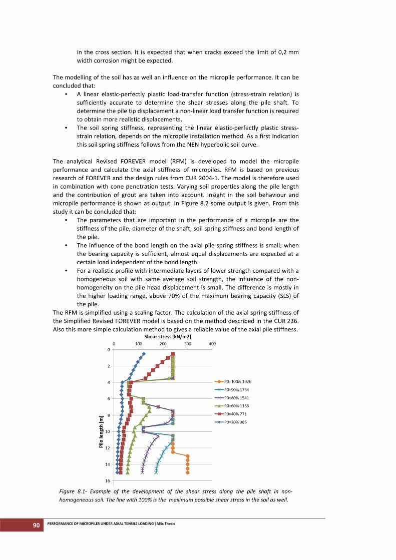
90 PERFORMANCE OF MICROPILES UNDER AXIAL TENSILE LOADING |MSc Thesis
in the cross section. It is expected that when cracks exceed the limit of 0,2 mm
width corrosion might be expected.
The modelling of the soil has as well an influence on the micropile performance. It can be
concluded that:
• A linear elastic-perfectly plastic load-transfer function (stress-strain relation) is
sufficiently accurate to determine the shear stresses along the pile shaft. To
determine the pile tip displacement a non-linear load transfer function is required
to obtain more realistic displacements.
• The soil spring stiffness, representing the linear elastic-perfectly plastic stress-
strain relation, depends on the micropile installation method. As a first indication
this soil spring stiffness follows from the NEN hyperbolic soil curve.
The analytical Revised FOREVER model (RFM) is developed to model the micropile
performance and calculate the axial stiffness of micropiles. RFM is based on previous
research of FOREVER and the design rules from CUR 2004-1. The model is therefore used
in combination with cone penetration tests. Varying soil properties along the pile length
and the contribution of grout are taken into account. Insight in the soil behaviour and
micropile performance is shown as output. In Figure 8.2 some output is given. From this
study it can be concluded that:
• The parameters that are important in the performance of a micropile are the
stiffness of the pile, diameter of the shaft, soil spring stiffness and bond length of
the pile.
• The influence of the bond length on the axial pile spring stiffness is small; when
the bearing capacity is sufficient, almost equal displacements are expected at a
certain load independent of the bond length.
• For a realistic profile with intermediate layers of lower strength compared with a
homogeneous soil with same average soil strength, the influence of the non-
homogeneity on the pile head displacement is small. The difference is mostly in
the higher loading range, above 70% of the maximum bearing capacity (SLS) of
the pile.
The RFM is simplified using a scaling factor. The calculation of the axial spring stiffness of
the Simplified Revised FOREVER model is based on the method described in the CUR 236.
Also this more simple calculation method to gives a reliable value of the axial pile stiffness.
Figure 8.1- Example of the development of the shear stress along the pile shaft in non-
homogeneous soil. The line with 100% is the maximum possible shear stress in the soil as well.
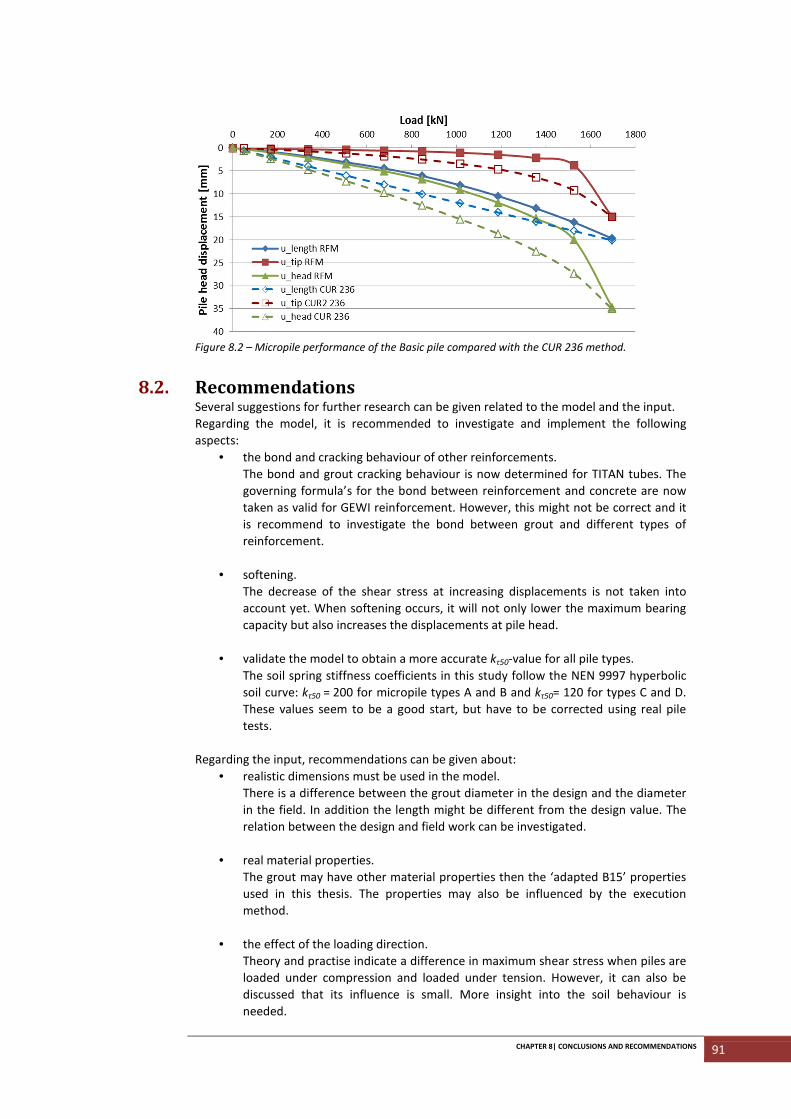
CHAPTER 8| CONCLUSIONS AND RECOMMENDATIONS 91
Figure 8.2 – Micropile performance of the Basic pile compared with the CUR 236 method.
8.2. Recommendations Several suggestions for further research can be given related to the model and the input.
Regarding the model, it is recommended to investigate and implement the following
aspects:
• the bond and cracking behaviour of other reinforcements.
The bond and grout cracking behaviour is now determined for TITAN tubes. The
governing formula’s for the bond between reinforcement and concrete are now
taken as valid for GEWI reinforcement. However, this might not be correct and it
is recommend to investigate the bond between grout and different types of
reinforcement.
• softening.
The decrease of the shear stress at increasing displacements is not taken into
account yet. When softening occurs, it will not only lower the maximum bearing
capacity but also increases the displacements at pile head.
• validate the model to obtain a more accurate kτ50-value for all pile types.
The soil spring stiffness coefficients in this study follow the NEN 9997 hyperbolic
soil curve: kτ50 = 200 for micropile types A and B and kτ50= 120 for types C and D.
These values seem to be a good start, but have to be corrected using real pile
tests.
Regarding the input, recommendations can be given about:
• realistic dimensions must be used in the model.
There is a difference between the grout diameter in the design and the diameter
in the field. In addition the length might be different from the design value. The
relation between the design and field work can be investigated.
• real material properties.
The grout may have other material properties then the ‘adapted B15’ properties
used in this thesis. The properties may also be influenced by the execution
method.
• the effect of the loading direction.
Theory and practise indicate a difference in maximum shear stress when piles are
loaded under compression and loaded under tension. However, it can also be
discussed that its influence is small. More insight into the soil behaviour is
needed.

CHAPTER 9| REFERENCES 93
REFERENCES
[Picture frontpage] Combitunnel Nijverdal, Volker InfraDesign
[1] FOREVER (2008), Synthesis of the Results and recommendations of the French National
Project on Micropiles (English translation), Dallas, Texas: ADSC
[2] API RP 2A-WSD (2000), Recommended Practice for Planning, Designing and
Construction Fixed Offshore Platforms - Working Stress Design, 21st edition, Washington:
API
[3] CUR 2001-4 (2001), Design rules for tension piles (Dutch), Gouda: CUR
[4] NEN-EN 14199 (2005), Execution of special geotechnical works – Micropiles (Dutch
norm), Delft: NEN
[5] Qian Z., Lu X., (2011), Behavior of Micropiles in Soft Soil under Vertical Loading,
Advanced Materials Research Vols. 243-249, pp. 2143-2150
[6] CUR 236 (2011), Ankerpalen, Gouda: CUR
[7] Personal communication with H.J. Everts, 28/2/2013
[8] NEN-EN 1992-1-1 +C2/NB (2011), National Annex to NEN-EN 1992-1-1+C2 Eurocode 2:
Design of concrete structures - Part 1-1: General rules and rules for buildings,NEN: Delft
[9] EN 10080 (2005), Steel for the reinforcement of concrete – Weldable reinforcing steel
NEN: Delft
[10] NEN-EN 1997-1 (2005), Eurocode 7: Geotechnical design, Part 1: General rules , Delft:
NEN
[11] NEN 9997-1+C1 (2012), Geotechnical design of structures – Part 1: General rules
(Dutch norm), Delft: NEN
[12] DIN1054 (2005), Subsoil - Verification of the safety of earthworks and foundations, (in
German) Berlin: DIN
[13] ISO 19902 (2006), Petroleum and Natural Gas Industries – Fixed steel offshore
structures
[14] Randolph, M., Fleming, K. et al (2009), Piling engineering, 3rd
edition, Oxon: Taylor &
Francis Group
[15] Randolph, M., Gourvenec, S. (2011), Offshore Geotechnical Engineering, Oxon: Taylor
& Francis Group
[16] Misra A., Chen C.-H. (2003), Analytical solution for micropile design under tension and
compression, Geotechnical and Geological Engineering nr.22, pp. 199-225
94 PERFORMANCE OF MICROPILES UNDER AXIAL TENSILE LOADING |MSc Thesis
[17] Randolph, M.F. (2003) Science and empiricism in pile foundation design,
Geotechnique 53, No10, pp. 847-875
[18] Yap, L.P., Rodger, A.A. (1984), A study of the behaviour of vertical rock anchors using
the finite element method, Int. J. Rock Mech Min Sci & Geomech Abstr, Vol21, No2, pp. 47-
61
[19] Randolph, M.F., and Wroth, C.P. (1978), Analysis of deformation of vertically loaded
piles, Journal of the Geotechnical Engineering Division, pp. 1465-1488
[20] Dalen, J.H. van, Opstal, A.Th (1994),. “Verankering van steile taluds”; syllabus
gezamenlijke studiedag KVIV en KIVI te Antwerpen
[21] Mylonakis, G. (2001), Winkler modulus for axially loaded piles, Geotechnique 51, No5,
p455-461
[22] BBRI (2008), Research projects on grout anchors, Proceedings international
symposium ground anchors Limelette test field results, Volume 2
[23] Lengkeek, H.J. (2009), stijfheid mechanisch gerolde ankers type C Presentation
[24] Jungwirth, J., Mutoni, A. (2004), Structural Behaviour of Tension Members in UHPC,
Structural concrete Laboratory, Lausanne, Switzerland
[25] Barbosa, M.T.G., De Souza Sanchez Filho, E., De Oliveira, T.M., Dos Santos, E.J. (2008)
Analysis of the Relative Rib Area of Reinforcing Bars Pull Out Tests, Materials Research,
Vol.11, No.4, pp. 453-457
[26] Personal communication with C. vd Veen, 31/1/2013, 23/4/2013 and 6/6/2013
[27] SAS manual
[28] Braam, C.R., Breugel, K. van, Veen, C. van der, Walraven, J.C. (2011) Concrete
Structures under Imposed Thermal and Shrinkage Deformations Theory and Practice, Delft:
Course-reader
[29] Ischebeck, E.F. (2010), The design and execution of drilled and flushed-grouted TITAN
micropiles, Presentation on the 10th
international workshop on micropiles, Washington,
USA
[30] Veen, C. van der (1990), Cryogenic bond stress-slip relationship Dissertation; TU Delft
[31] Lam, C., Jefferis, S.A. (2011), Critical assessment of pile modulus determination
methods, Canadian Geotechnical Journal, No.48, pp 1433-1448
[32] Lehane, B., Jardine, R., Bond, A., and Frank, R. (1993). Mechanisms of Shaft Friction in
Sand from Instrumented Pile Tests. J. Geotechnical Engineering 119(1), pp. 19–35.
[33] Fellenius, B.H. (2002), Side resistance in piles and drilled shafts. Discussion, ASCE
Journal of Geotechnical and Geoenvironmental engineering, Vol.128, No.5, pp. 446-448
[34] Axelsson, G. (2000). Long-term set-up of driven piles in sand. Stockholm: Royal
Institute of Technology.
[35] Muir Wood, D. (2004). Geotechnical Modeling. Version 2.2.
CHAPTER 9| REFERENCES 95
[36] FHWA (2006), A Laboratory and Field Study of Composite Piles for Bridge
Substructures, pp. 28-63 USA
[37] Guo, W.D., Randolph, M.F. (1997), Vertically loaded piles in non-homogeneous media,
International journal for numerical and analytical methods in Geomechanics, Vol21, pp.
507-523
[38] Liu, J., Xiao, H.B., Tang, J., Li, Q.S. (2004), Analysis of load transfer of single pile in
layered soil, Computers and Geotechnics 31, pp. 127-135
[39] Ai Z.Y., Yue Z.Q. (2008) Elastic analysis of axially loaded single pile in multi-layered
soils, International Journal of Engineering Science 47, pp. 1079–1088
[40] Vriend, A., (2013) Toelichting rekenmodel AVR tbv Axiale Veerstijfheid Memo