Embed Size (px)
Citation preview

Performance of UAV Radar Concepts
for Naval Defence 11aw12 Final Report
Peter W. Moo
TECHNICAL REPORT
DRDC Ottawa TR 2008-340
March 2009


Performance of UAV Radar Concepts for Naval
Defence11aw12 Final Report
Peter W. Moo
Defence R&D Canada – Ottawa
Defence R&D Canada – Ottawa
Technical Report
DRDC Ottawa TR 2008-340
March 2009

Principal Author
Original signed by Peter W. Moo
Peter W. Moo
Approved by
Original signed by D. Dyck
D. Dyck
Head/RS
Approved for release by
Original signed by P. Lavoie
P. Lavoie
Head/Document Review Panel
c© Her Majesty the Queen in Right of Canada as represented by the Minister of National
Defence, 2009
c© Sa Majeste la Reine (en droit du Canada), telle que representee par le ministre de la
Defense nationale, 2009

Abstract
This report analyzes the performance of a bistatic uninhabited aerial vehicle (UAV) radar
to detect cruise missile threats beyond a ship’s horizon. The bistatic system, together with
adaptive signal processing is shown to provide self-defence capabilities against targets that
are heading towards the ship. For area air defence, the UAV radar may not be able to detect
some targets, depending on the bistatic geometry. A monostatic UAV radar for small boat
defence is also developed. The radar cross section (RCS) of a small boat is modelled,
and it is shown that the median monostatic RCS is 1 m2. Performance of the UAV radar
is analyzed by simulating the small boat scenario in RLSTAP. With the use of Factored
space-time adaptive processing (STAP) to reduce clutter power, the resulting minimum
detectable velocity is shown to be between 2.8 m/s and 3.8 m/s. Payload sizes and weights
are estimated for the proposed radars.
Resume
Le present rapport analyse les performances d’un radar bistatique d’UAV utilise pour
detecter des menaces sous forme de missiles de croisiere au-dela de l’horizon d’un na-
vire. On montre que le systeme bistatique, combine au traitement de signaux adaptatif,
offre des capacites d’autodefense contre des cibles qui s’approchent du navire. Aux fins de
la defense aerienne sectorielle, il se peut que le radar d’UAV ne soit pas capable de detecter
certaines cibles, tout dependant de la geometrie bistatique. Un radar monostatique d’UAV
servant a la defense contre les petits bateaux est egalement en cours de developpement.
La surface equivalente radar (SER) d’un petit bateau est modelise, et l’on montre que la
SER monostatique moyenne est de 1 m2. Les performances du radar d’UAV sont analysees
par simulation du scenario d’un petit bateau dans RLSTAP. Grace a l’utilisation du traite-
ment STAP pondere pour reduire la puissance du clutter, on montre que la vitesse minimale
detectable resultante est comprise entre 2,8 m/s et 3,8 m/s.
DRDC Ottawa TR 2008-340 i

This page intentionally left blank.
ii DRDC Ottawa TR 2008-340
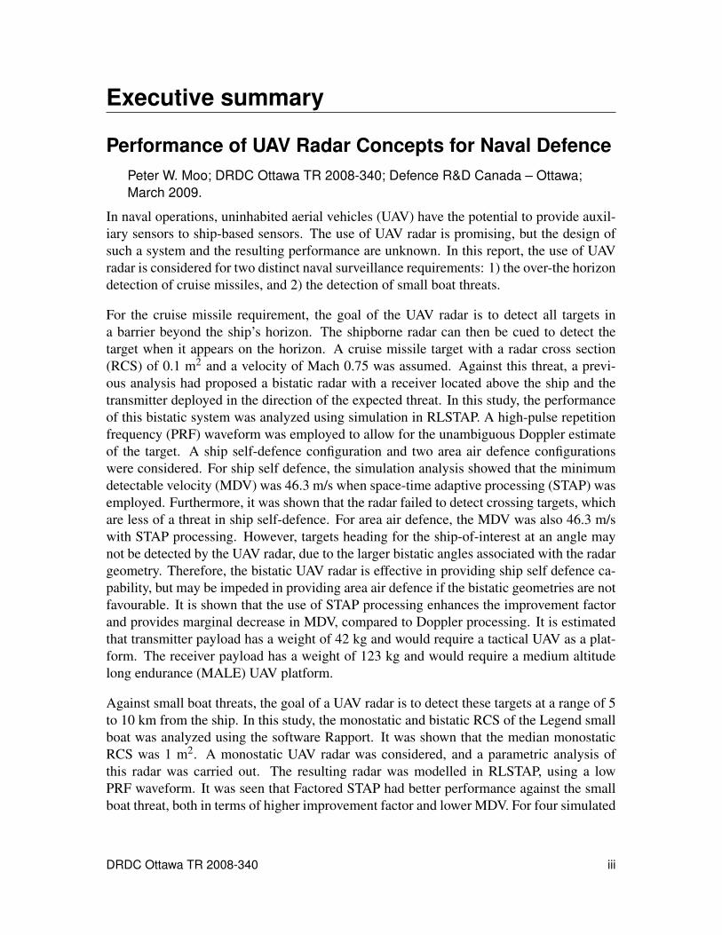
Executive summary
Performance of UAV Radar Concepts for Naval Defence
Peter W. Moo; DRDC Ottawa TR 2008-340; Defence R&D Canada – Ottawa;
March 2009.
In naval operations, uninhabited aerial vehicles (UAV) have the potential to provide auxil-
iary sensors to ship-based sensors. The use of UAV radar is promising, but the design of
such a system and the resulting performance are unknown. In this report, the use of UAV
radar is considered for two distinct naval surveillance requirements: 1) the over-the horizon
detection of cruise missiles, and 2) the detection of small boat threats.
For the cruise missile requirement, the goal of the UAV radar is to detect all targets in
a barrier beyond the ship’s horizon. The shipborne radar can then be cued to detect the
target when it appears on the horizon. A cruise missile target with a radar cross section
(RCS) of 0.1 m2 and a velocity of Mach 0.75 was assumed. Against this threat, a previ-
ous analysis had proposed a bistatic radar with a receiver located above the ship and the
transmitter deployed in the direction of the expected threat. In this study, the performance
of this bistatic system was analyzed using simulation in RLSTAP. A high-pulse repetition
frequency (PRF) waveform was employed to allow for the unambiguous Doppler estimate
of the target. A ship self-defence configuration and two area air defence configurations
were considered. For ship self defence, the simulation analysis showed that the minimum
detectable velocity (MDV) was 46.3 m/s when space-time adaptive processing (STAP) was
employed. Furthermore, it was shown that the radar failed to detect crossing targets, which
are less of a threat in ship self-defence. For area air defence, the MDV was also 46.3 m/s
with STAP processing. However, targets heading for the ship-of-interest at an angle may
not be detected by the UAV radar, due to the larger bistatic angles associated with the radar
geometry. Therefore, the bistatic UAV radar is effective in providing ship self defence ca-
pability, but may be impeded in providing area air defence if the bistatic geometries are not
favourable. It is shown that the use of STAP processing enhances the improvement factor
and provides marginal decrease in MDV, compared to Doppler processing. It is estimated
that transmitter payload has a weight of 42 kg and would require a tactical UAV as a plat-
form. The receiver payload has a weight of 123 kg and would require a medium altitude
long endurance (MALE) UAV platform.
Against small boat threats, the goal of a UAV radar is to detect these targets at a range of 5
to 10 km from the ship. In this study, the monostatic and bistatic RCS of the Legend small
boat was analyzed using the software Rapport. It was shown that the median monostatic
RCS was 1 m2. A monostatic UAV radar was considered, and a parametric analysis of
this radar was carried out. The resulting radar was modelled in RLSTAP, using a low
PRF waveform. It was seen that Factored STAP had better performance against the small
boat threat, both in terms of higher improvement factor and lower MDV. For four simulated
DRDC Ottawa TR 2008-340 iii

scenarios, Factored STAP resulted in MDVs between 2.8 m/s and 3.8 m/s. The use of STAP
provides significant benefit in the detection of small boats by decreasing the MDV. Further
work in this area would involve verifying UAV radar performance using experimental data.
For small boat detection, the radar payload has an estimated weight of 67 kg and would
require a tactical UAV as a platform.
iv DRDC Ottawa TR 2008-340

Sommaire
Performance of UAV Radar Concepts for Naval Defence
Peter W. Moo ; DRDC Ottawa TR 2008-340 ; R & D pour la defense Canada –
Ottawa ; mars 2009.
En operations navales, les vehicules aeriens teleguides (UAV) ont le potentiel de fournir
des capteurs auxiliaires aux capteurs a bord des navires. L’utilisation du radar d’UAV est
prometteuse, mais la conception d’un tel systeme et les performances resultantes sont in-
connues. Dans le present rapport, l’utilisation du radar d’UAV est envisagee pour deux exi-
gences de surveillance navale distinctes : 1) detection transhorizon de missiles de croisiere ;
2) detection de menaces sous forme de petits bateaux.
Quant a l’exigence relative a la detection de missiles de croisiere, le radar d’UAV a pour
but de detecter toutes les cibles dans une barriere au-dela de l’horizon du navire. Le ra-
dar de navire peut ensuite tre prepare pour detecter la cible lorsqu’elle apparat a l’horizon.
On a presume comme cible un missile de croisiere d’une SER de 0,1 m2 et se deplaant
a une vitesse de Mach 0,75. Pour detecter une telle menace, une analyse anterieure avait
propose un radar bistatique avec une antenne de reception situee au-dessus du navire et
une antenne d’emission orientee dans la direction de la menace prevue. Dans la presente
etude, les performances de ce systeme bistatique sont analysees au moyen d’une simula-
tion dans RLSTAP. Une forme d’onde a haute FRI est utilisee pour permettre l’estimation
Doppler sans ambigute de la cible. On a etudie une configuration d’autodefense de navire
et deux configurations de defense aerienne. Aux fins de l’autodefense du navire, l’analyse
de simulation montre que la vitesse minimale detectable (MDV) est de 46,3 m/s lorsque
le traitement STAP est utilise. En outre, on montre que le radar n’a pas reussi a detecter
les cibles traversantes, qui sont une menace moindre pour l’autodefense des navires. En
defense aerienne sectorielle, la MDV est egalement de 46,3 m/s avec traitement STAP.
Toutefois, les cibles se rapprochant du navire d’intert a un certain angle peuvent ne pas
tre detectees par le radar d’UAV, a cause des angles bistatique plus grands associes a la
geometrie du radar. Par consequent, le radar bistatique d’UAV est efficace dans la mesure
o il augmente la capacite d’autodefense du navire, mais peut tre d’une efficacite limitee
en termes de defense aerienne sectorielle si la geometrie bistatique n’est pas favorable. On
montre que l’utilisation du traitement STAP augmente le facteur d’amelioration et entrane
une legere reduction de la MDV, comparativement au traitement Doppler.
Dans le cas des menaces sous forme de petits bateaux, le radar d’UAV a pour but de detecter
ces cibles a une distance de 5 a 10 km du navire. Dans la presente etude, les SER monosta-
tique et bistatique du petit bateau Legend sont analysees au moyen du logiciel Rapport. Il
est montre que la SER monostatique moyenne est de 1 m2. On a envisage un radar mono-
statique d’UAV et effectue une analyse parametrique de ce radar. Le radar a ete modelise
dans RLSTAP, au moyen d’une forme d’onde a basse FRI. On a constate que le traitement
DRDC Ottawa TR 2008-340 v

STAP pondere avait de meilleures performances vis-a-vis de la menace sous forme d’un
petit bateau, a la fois en augmentant le facteur d’amelioration et en reduisant la MDV. Pour
les quatre scenarios de simulation, le traitement STAP pondere a donne lieu a des MDV
comprises entre 2,8 m/s et 3,8 m/s. L’utilisation du traitement STAP donne un avantage
considerable dans la detection de petits bateaux grace a la reduction de la MDV. Les re-
cherches futures dans ce domaine consisteraient a verifier les performances du radar d’UAV
au moyen de donnees experimentales.
vi DRDC Ottawa TR 2008-340

Table of contents
Abstract . . . . . . . . . . . . . . . . . . . . . . . . . . . . . . . . . . . . . . . . . i
Resume . . . . . . . . . . . . . . . . . . . . . . . . . . . . . . . . . . . . . . . . . i
Executive summary . . . . . . . . . . . . . . . . . . . . . . . . . . . . . . . . . . . iii
Sommaire . . . . . . . . . . . . . . . . . . . . . . . . . . . . . . . . . . . . . . . . v
Table of contents . . . . . . . . . . . . . . . . . . . . . . . . . . . . . . . . . . . . vii
List of figures . . . . . . . . . . . . . . . . . . . . . . . . . . . . . . . . . . . . . . ix
List of tables . . . . . . . . . . . . . . . . . . . . . . . . . . . . . . . . . . . . . . . xiii
1 Introduction . . . . . . . . . . . . . . . . . . . . . . . . . . . . . . . . . . . . . 1
2 Cruise Missile Threats . . . . . . . . . . . . . . . . . . . . . . . . . . . . . . . 3
3 Bistatic Radar Concept . . . . . . . . . . . . . . . . . . . . . . . . . . . . . . . 4
4 Sea clutter modelling and prediction . . . . . . . . . . . . . . . . . . . . . . . . 9
4.1 Walker model for sea clutter Doppler spectrum . . . . . . . . . . . . . . . 9
4.2 Prediction of minimum detectable velocity for targets in sea clutter . . . . 10
5 Simulation and Processing . . . . . . . . . . . . . . . . . . . . . . . . . . . . . 15
5.1 RLSTAP . . . . . . . . . . . . . . . . . . . . . . . . . . . . . . . . . . . 15
5.2 Space-Time Adaptive Processing . . . . . . . . . . . . . . . . . . . . . . 19
6 Concept Performance . . . . . . . . . . . . . . . . . . . . . . . . . . . . . . . . 22
6.1 Ship Self-Defence . . . . . . . . . . . . . . . . . . . . . . . . . . . . . . 22
6.2 Area Air Defence, Configuration 1 . . . . . . . . . . . . . . . . . . . . . 31
6.3 Area Air Defence, Configuration 2 . . . . . . . . . . . . . . . . . . . . . 36
6.4 Discussion . . . . . . . . . . . . . . . . . . . . . . . . . . . . . . . . . . 37
7 Small Boat Radar Cross Section . . . . . . . . . . . . . . . . . . . . . . . . . . 42
8 Assessment of Small Boat Detection Performance . . . . . . . . . . . . . . . . . 45
DRDC Ottawa TR 2008-340 vii

9 Simulation of UAV Detection of Small Boats . . . . . . . . . . . . . . . . . . . 50
10 Payload Considerations . . . . . . . . . . . . . . . . . . . . . . . . . . . . . . . 54
10.1 Bistatic radar for cruise missile detection . . . . . . . . . . . . . . . . . . 54
10.2 Monostatic radar for small boat detection . . . . . . . . . . . . . . . . . . 55
11 Conclusions . . . . . . . . . . . . . . . . . . . . . . . . . . . . . . . . . . . . . 57
Annex A: Bistatic Small Boat RCS . . . . . . . . . . . . . . . . . . . . . . . . . . 59
References . . . . . . . . . . . . . . . . . . . . . . . . . . . . . . . . . . . . . . . . 63
viii DRDC Ottawa TR 2008-340

List of figures
Figure 1: Illustration of monostatic and bistatic UAV radar concepts. . . . . . . . . 4
Figure 2: Minimum receiver antenna diameter as a function of receiver ground
range. . . . . . . . . . . . . . . . . . . . . . . . . . . . . . . . . . . . . 7
Figure 3: Minimum receiver antenna diameter as a function of CPI length. . . . . . 7
Figure 4: Required antenna dimensions for detection of a 0.01m2 target at a
receiver ground range of 30 km, for various values of peak transmitter
power. Transmitter and receiver antennas are square planar arrays. . . . . 8
Figure 5: Doppler spectrum of upwind sea clutter, based on Walker model. . . . . 11
Figure 6: Doppler spectrum of downwind sea clutter, based on Walker model. . . . 11
Figure 7: Geometry of bistatic radar, illustrating target velocity vector V, bistatic
angle β, and angle δ between velocity vector and bisector of bistatic angle. 12
Figure 8: Detectable geometries for bistatic concept using analytical MDV. . . . . 13
Figure 9: Prediction of clutter Doppler and range extent when the transmitter
azimuth angle is 0˚ and velocity is 50 m/s. . . . . . . . . . . . . . . . . . 14
Figure 10: Top level of RLSTAP workspace for UAV radar lineup. . . . . . . . . . . 16
Figure 11: Expanded view of Initialization glyph. . . . . . . . . . . . . . . . . . . 16
Figure 12: Expanded view of PRI Loop glyph. . . . . . . . . . . . . . . . . . . . . 17
Figure 13: Site-specific clutter model for littoral region near Maine. . . . . . . . . . 18
Figure 14: σ0 as a function of grazing angle, when λ = 0.03m, Φ=90˚, τ = 2µs,
and γa = 0.0265 rad. . . . . . . . . . . . . . . . . . . . . . . . . . . . . 19
Figure 15: Top-down view of missile trajectory through rectangular detection barrier. 23
Figure 16: Top-down view of UAV radar configuration for ship self-defence. . . . . 23
Figure 17: Range-Doppler map of returns from Scenario A with littoral
background and Sea State 3. . . . . . . . . . . . . . . . . . . . . . . . . 26
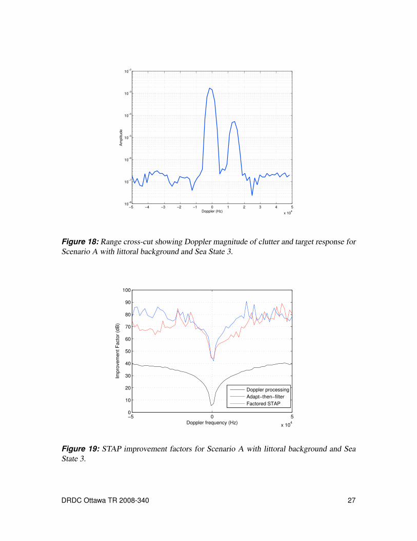
Figure 18: Range cross-cut showing Doppler magnitude of clutter and target
response for Scenario A with littoral background and Sea State 3. . . . . 27
DRDC Ottawa TR 2008-340 ix

Figure 19: STAP improvement factors for Scenario A with littoral background and
Sea State 3. . . . . . . . . . . . . . . . . . . . . . . . . . . . . . . . . . 27
Figure 20: STAP improvement factors for Scenario A with sea clutter background
and Sea State 5. . . . . . . . . . . . . . . . . . . . . . . . . . . . . . . . 28
Figure 21: Comparison of Adapt-then-filter improvement factors for various
clutter backgrounds for Scenario A. . . . . . . . . . . . . . . . . . . . . 28
Figure 22: Comparison of Factored STAP improvement factors for various clutter
backgrounds for Scenario A. . . . . . . . . . . . . . . . . . . . . . . . . 29
Figure 23: Range-Doppler map of radar returns from Scenario B with littoral
background and Sea State 3. . . . . . . . . . . . . . . . . . . . . . . . . 29
Figure 24: STAP improvement factors for Scenario B with littoral background and
Sea State 3. . . . . . . . . . . . . . . . . . . . . . . . . . . . . . . . . . 30
Figure 25: STAP improvement factors for Scenario C with littoral background and
Sea State 3. . . . . . . . . . . . . . . . . . . . . . . . . . . . . . . . . . 30
Figure 26: Detectable geometries for bistatic concept using MDV derived from
simulations. . . . . . . . . . . . . . . . . . . . . . . . . . . . . . . . . . 31
Figure 27: Top-down view of area air defence, configuration 1. . . . . . . . . . . . 33
Figure 28: Range-Doppler map of returns from Scenario D with littoral
background and Sea State 3. . . . . . . . . . . . . . . . . . . . . . . . . 33
Figure 29: STAP improvement factors for Scenario D with littoral background and
Sea State 3. . . . . . . . . . . . . . . . . . . . . . . . . . . . . . . . . . 34
Figure 30: Comparison of Adapt-then-filter improvement factors for various
clutter backgrounds for Scenario D. . . . . . . . . . . . . . . . . . . . . 34
Figure 31: Comparison of Factored STAP improvement factors for various clutter
backgrounds for Scenario D. . . . . . . . . . . . . . . . . . . . . . . . . 35
Figure 32: STAP improvement factors for Scenario E with littoral background and
Sea State 3. . . . . . . . . . . . . . . . . . . . . . . . . . . . . . . . . . 35
Figure 33: STAP improvement factors for Scenario F with littoral background and
Sea State 3. . . . . . . . . . . . . . . . . . . . . . . . . . . . . . . . . . 36
Figure 34: Top-down view of area air defence, configuration 2. . . . . . . . . . . . 38
x DRDC Ottawa TR 2008-340

Figure 35: Range-Doppler map of returns from Scenario G with littoral
background and Sea State 3. . . . . . . . . . . . . . . . . . . . . . . . . 39
Figure 36: STAP improvement factors for Scenario G with littoral background and
Sea State 3. . . . . . . . . . . . . . . . . . . . . . . . . . . . . . . . . . 39
Figure 37: Comparison of Adapt-then-filter improvement factors for various
clutter backgrounds for Scenario G. . . . . . . . . . . . . . . . . . . . . 40
Figure 38: Comparison of Factored STAP improvement factors for various clutter
backgrounds for Scenario G. . . . . . . . . . . . . . . . . . . . . . . . . 40
Figure 39: STAP improvement factors for Scenario H with littoral background and
Sea State 3. . . . . . . . . . . . . . . . . . . . . . . . . . . . . . . . . . 41
Figure 40: STAP improvement factors for Scenario I with littoral background and
Sea State 3. . . . . . . . . . . . . . . . . . . . . . . . . . . . . . . . . . 41
Figure 41: The Legend small boat and CAD model. . . . . . . . . . . . . . . . . . 42
Figure 42: Coordinate system for bistatic RCS modelling. . . . . . . . . . . . . . . 43
Figure 43: SIR versus antenna width for a square antenna, P = 1.5kW , Rg = 10km. . 47
Figure 44: SIR versus ground range for P = 1.5kW and a 0.5 m by 0.5 m antenna. . 48
Figure 45: SIR versus peak power for Rg = 10km and a 0.5 m by 0.5 m antenna. . . 48
Figure 46: SIR versus wave height for P = 1.5kW , Rg = 10km and a 0.5 m by 0.5
m antenna. . . . . . . . . . . . . . . . . . . . . . . . . . . . . . . . . . 49
Figure 47: Range-Doppler map of returns from Scenario 1. . . . . . . . . . . . . . 51
Figure 48: STAP improvement factors for Scenario 1. . . . . . . . . . . . . . . . . 52
Figure 49: STAP improvement factors for Scenario 2. . . . . . . . . . . . . . . . . 52
Figure 50: STAP improvement factors for Scenario 3. . . . . . . . . . . . . . . . . 53
Figure 51: STAP improvement factors for Scenario 4. . . . . . . . . . . . . . . . . 53
Figure A.1: Bistatic RCS in dBsm when the transmitter location is specified by
θi=10˚ and φi=0˚. . . . . . . . . . . . . . . . . . . . . . . . . . . . . . . 59
Figure A.2: Bistatic RCS in dBsm when the transmitter location is specified by
θi=30˚ and φi=0˚. . . . . . . . . . . . . . . . . . . . . . . . . . . . . . . 60
DRDC Ottawa TR 2008-340 xi

Figure A.3: Bistatic RCS in dBsm when the transmitter location is specified by
θi=60˚ and φi=0˚. . . . . . . . . . . . . . . . . . . . . . . . . . . . . . . 60
Figure A.4: Bistatic RCS in dBsm when the transmitter location is specified by
θi=89˚ and φi=0˚. . . . . . . . . . . . . . . . . . . . . . . . . . . . . . . 61
Figure A.5: RCS statistics for 10 GHz, VV polarization. Monostatic RCS values
are indicated by asterisks. . . . . . . . . . . . . . . . . . . . . . . . . . 62
xii DRDC Ottawa TR 2008-340

List of tables
Table 1: Radar system parameters for over-the-horizon cruise missile detection. . 6
Table 2: Walker model parameters for X-band radar data. . . . . . . . . . . . . . 10
Table 3: Simulation scenarios for ship self-defence configuration. . . . . . . . . . 24
Table 4: Simulation scenarios for area air defence, configuration 1. . . . . . . . . 31
Table 5: Simulation scenarios for area air defence, configuration 2. . . . . . . . . 36
Table 6: Monostatic RCS of the Legend small boat, for transmitter locations
specified by θi and φi. . . . . . . . . . . . . . . . . . . . . . . . . . . . 44
Table 7: Radar system parameters for small boat detection. . . . . . . . . . . . . 45
Table 8: Simulation scenarios for UAV radar detection of small boats. . . . . . . . 50
Table 9: Minimum detectable velocity (MDV) and usable Doppler space
fraction (UDSF) for small boat detection scenarios. . . . . . . . . . . . . 51
Table 10: Payload description for the Raytheon SeaVue radar. . . . . . . . . . . . 54
Table 11: Payload estimate for the bistatic radar for cruise missile detection. . . . . 55
Table 12: Payload estimate for the monostatic radar for small boat detection. . . . . 56
DRDC Ottawa TR 2008-340 xiii

This page intentionally left blank.
xiv DRDC Ottawa TR 2008-340

1 Introduction
In naval operations, uninhabited aerial vehicles (UAV) have the potential to provide auxil-
iary sensors to ship-based sensors. The use of UAV radar is promising, but the design of
such a system and the resulting performance are unknown. In this report, the use of UAV
radar is considered for two distinct naval surveillance requirements: 1) the over-the horizon
detection of cruise missiles, and 2) the detection of small boat threats.
The first requirement is for increased warning time against low-altitude cruise missile
threats that originate from beyond the horizon. Such threats are particularly dangerous
when they operate at high velocities and thus result in very short reaction times for a ves-
sel’s surveillance system once the threats appear on the horizon. When operating in the
littoral, naval vessels may encounter threats launched from other ships or land-based ve-
hicles. The aim of the first part of this work is to develop an affordable UAV-based radar
system that will provide over-the-horizon detection capability.
There are two general scenarios of interest for cruise missile defence, the blue water sce-
nario and the littoral scenario. In the blue water scenario, a vessel is located in the middle
of open ocean. Land-based threats are not present, and in general there is not a lot of naval
traffic in these areas. The primary source of interference for radar detection is sea clutter
at various sea states. In the littoral scenario, a vessel is up to 100 km from shore. Threats
may originate from other naval vessels or land vessels. Significant amounts of coastal
traffic may be present. Both sea and land clutter may provide sources of interference for
radar detection.
A UAV-based early detection system has several potential functionalities. It could be used
as a barrier search detection scheme. If a target is detected within the barrier, the UAV
system would cue the shipborne radar regarding an imminent threat. It could also provide
tracking capability or be used to provide illumination for missile guidance. In this study
attention is restricted to the barrier search detection capability.
The shipborne radar horizon for a Canadian Patrol Frigate is approximately 20 to 25 km.
This value was determined from empirical evidence and verified by theory. In this study,
monostatic and bistatic UAV radar systems will be designed to detect threats at a range of
25 km and beyond.
The second naval requirement involves the defence of large naval vessels against small boat
threats. These threats may be loaded with explosives which can inflict significant damage
on a ship. Small boat threats range in size from jet skis to larger pleasure craft and may be
travelling at any speed. In order to contend with these threats, it will be necessary to detect
and track them and determine their intent, at a range of 5 to 10 km from the ship.
Previous work has shown that a target with 10 m2 radar cross section (RCS) in Sea State 1
can be detected with a navigation radar at a range of 5 to 10 km [1]. However, the detection
DRDC Ottawa TR 2008-340 1

of smaller targets in higher sea states remains a challenging problem. In general, shipborne
radars are unable to detect small boats with 1 m2 RCS. The goal of the second part of this
study is to develop a UAV radar system that will detect small boats.
In this report, the design and performance analysis of a UAV radar for over-the-horizon
cruise missile detection are presented in Sections 2-6. In Section 2 an overview of current
cruise missile threats is presented. Section 3 specifies the bistatic radar concept that will
be modelled and discusses tradeoffs in parameter selection. In Section 4 a theoretical
analysis of the Doppler extent of sea clutter is carried out. Section 5 presents an overview
of RLSTAP and the space-time adaptive processing techniques that will be used in this
study. In Section 6 the performance of the bistatic radar concept is studied using RLSTAP
simulations for ship self-defence and area air defence configurations.
UAV radar has not widely studied in the literature. Previous studies have considered the
use of SAR imaging from UAV platforms using millimeter wave radar [2], [3]. Tsunoda et
al. [4] describe Lynx, a SAR/MTI radar for UAV platforms that operates at Ku-band. Lynx
is produced by General Atomics and does not carry out clutter cancellation to decrease
minimum detectable velocity. The use of bistatic UAV configurations and the use of clutter
cancellation techniques has not been previously considered.
In Sections 7-9 the design and performance of a UAV radar for small boat detection are
given. Section 7 presents an analysis of the monostatic and bistatic RCS of the Legend
small boat. In Section 8 various tradeoffs in UAV radar design are considered. Section 9
examines the performance of a monostatic UAV radar for small boat detection using RL-
STAP simulation. UAV payload considerations are discussed in Section 10. Conclusions
are presented in Section 11.
2 DRDC Ottawa TR 2008-340

2 Cruise Missile Threats
In both the blue water and littoral scenarios, a naval vessel may encounter a number of
low-altitude threats that originate from beyond the horizon, including anti-ship missiles,
cruise missiles and low-flying aircraft. This section describes these threats.
An ever-present threat to naval vessels are anti-ship missiles (ASM). Generally, ASMs are
capable of cruising at low altitudes, travelling at subsonic or supersonic speeds, and can be
launched from a ship, a land vessel or an aircraft. There are numerous types of ASMs in
production, and they are used by almost every nation in the world. One example of an ASM
is the Russian SS-N-22 ‘Sunburn’, also called the ‘3M80’ or ‘Moskit’ [5]. The Moskit is a
surface-to-surface missile with inertial guidance, a dual mode active/passive radar terminal
seeker, and an electronic protection measure (EPM) capability. With a launch weight of
4,500 kg, the Moskit has a length of 9.74 m, a body diameter of 0.76 m and a wing span of
2.1 m. When cruising at low-altitudes, the Moskit has a range of approximately 150 km
and a cruise speed of approximately Mach 2.1. Another example of an ASM is Boeing’s
AGM-84 Harpoon [6], which has an air-launched model and a surface and submarine-
launched model. The Harpoon is lighter and smaller than the Moskit, with a weight of
519 kg, a length of 3.8 m, a body diameter of 0.34 m, and a wing span of 0.83 m. At low
altitudes, the Harpoon has a range of up to 124 km with a maximum speed of Mach 0.85.
Cruise missiles are surface-to-surface missiles that typically travel at subsonic speeds. One
common example is the Tomahawk cruise missile, which has a length of 6.25 m, a diameter
of 0.51 m, and a wing span of 2.62 m. The Tomahawk has a weight of 1,450 kg, a range of
1,300 km and a maximum speed of Mach 0.75 [7]. Previous work has been carried out on
analyzing the monostatic and bistatic radar cross section (RCS) of a cruise missile [8].
Anti-ship missiles and cruise missiles are especially challenging threats because of their
high velocity and low RCS. Low-flying aircraft are also threats of interest, because they
can be used as vehicles for delivering cruise or anti-ship missiles.
This study focuses on the anti-ship missile and cruise missile threats. The radar concepts
proposed will be evaluated against a generic missile target that has an RCS of 0.1 m2 with a
velocity of Mach 0.75. These characteristics are representative of a subsonic cruise missile.
An important goal of this work is to increase the reaction time against cruise missile threats.
It is assumed that the shipborne radar detects missile threats at a range of 20 km. Detecting
a cruise missile beyond the ship’s horizon increases the detection range and the reaction
time for the ship.
DRDC Ottawa TR 2008-340 3
3 Bistatic Radar Concept
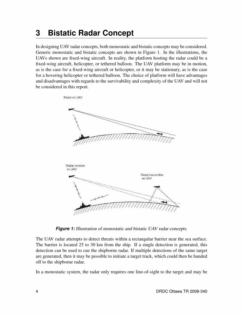
In designing UAV radar concepts, both monostatic and bistatic concepts may be considered.
Generic monostatic and bistatic concepts are shown in Figure 1. In the illustrations, the
UAVs shown are fixed-wing aircraft. In reality, the platform hosting the radar could be a
fixed-wing aircraft, helicopter, or tethered balloon. The UAV platform may be in motion,
as is the case for a fixed-wing aircraft or helicopter, or it may be stationary, as is the case
for a hovering helicopter or tethered balloon. The choice of platform will have advantages
and disadvantages with regards to the survivability and complexity of the UAV and will not
be considered in this report.
Figure 1: Illustration of monostatic and bistatic UAV radar concepts.
The UAV radar attempts to detect threats within a rectangular barrier near the sea surface.
The barrier is located 25 to 30 km from the ship. If a single detection is generated, this
detection can be used to cue the shipborne radar. If multiple detections of the same target
are generated, then it may be possible to initiate a target track, which could then be handed
off to the shipborne radar.
In a monostatic system, the radar only requires one line-of-sight to the target and may be
4 DRDC Ottawa TR 2008-340

designed to have a multifunction capability. However, a multifunction radar will generally
result in a large UAV payload. The goal of reducing the UAV payload leads to the consider-
ation of bistatic UAV concepts. In a bistatic system, a UAV transmitter is deployed beyond
the horizon, in the proximity of the anticipated threat. The UAV receiver would be located
directly above the ship. One advantage of such a bistatic system is that the closer prox-
imity of the transmitter to the target enhances signal-to-noise ratio. Another advantage
is that such a system may allow for simpler and cheaper UAV payloads, especially at the
transmitter. The reduction in transmitter range may also reduce the power requirements at
the transmitter. However, such a bistatic system would require synchronization between
the transmitter and receiver to achieve coherent processing gains. Furthermore, a bistatic
system requires two lines-of-sight to the target.
A number of monostatic and bistatic concepts were proposed and analyzed in [9]. For
each concept the tradeoff between radar parameters was studied, and the performance of
the various radar concepts was compared. As a result of the analysis it was determined
that a bistatic radar concept had the best tradeoff between performance and payload size
and therefore is the concept considered for this study. The bistatic radar concept and its
analysis are summarized in the following.
The bistatic concept has a receiver located above the ship and a transmitter deployed in
the direction of the barrier. The transmit antenna scans, in azimuth only, the designated
barrier. The scanning may be done mechanically or electronically, and it is assumed that
the antenna steers up to ± 60˚ in azimuth. Steering in azimuth only reduces the complexity
of the transmitter and may result in a smaller and lighter UAV payload. The inner edge of
the barrier is 5 km in ground range from the transmitter, and the barrier has a width of 5 km.
There are a number of radar parameters that may be traded off while maintaining desired
radar detection performance. It is assumed that probability of detection (Pd) is 0.9 and
probability of false alarm (Pf a) is 10−6. Table 1 gives the bistatic radar system parameters
used in this study.
The signal-to-noise ratio (SNR) for a bistatic radar with coherent integration is given by
the bistatic radar range equation.
S
N= NP
PτGT σAe
(4π)2R2T R2
RkT0BFnLs
. (1)
From this equation, various parameter values that achieve a given SNR can be computed.
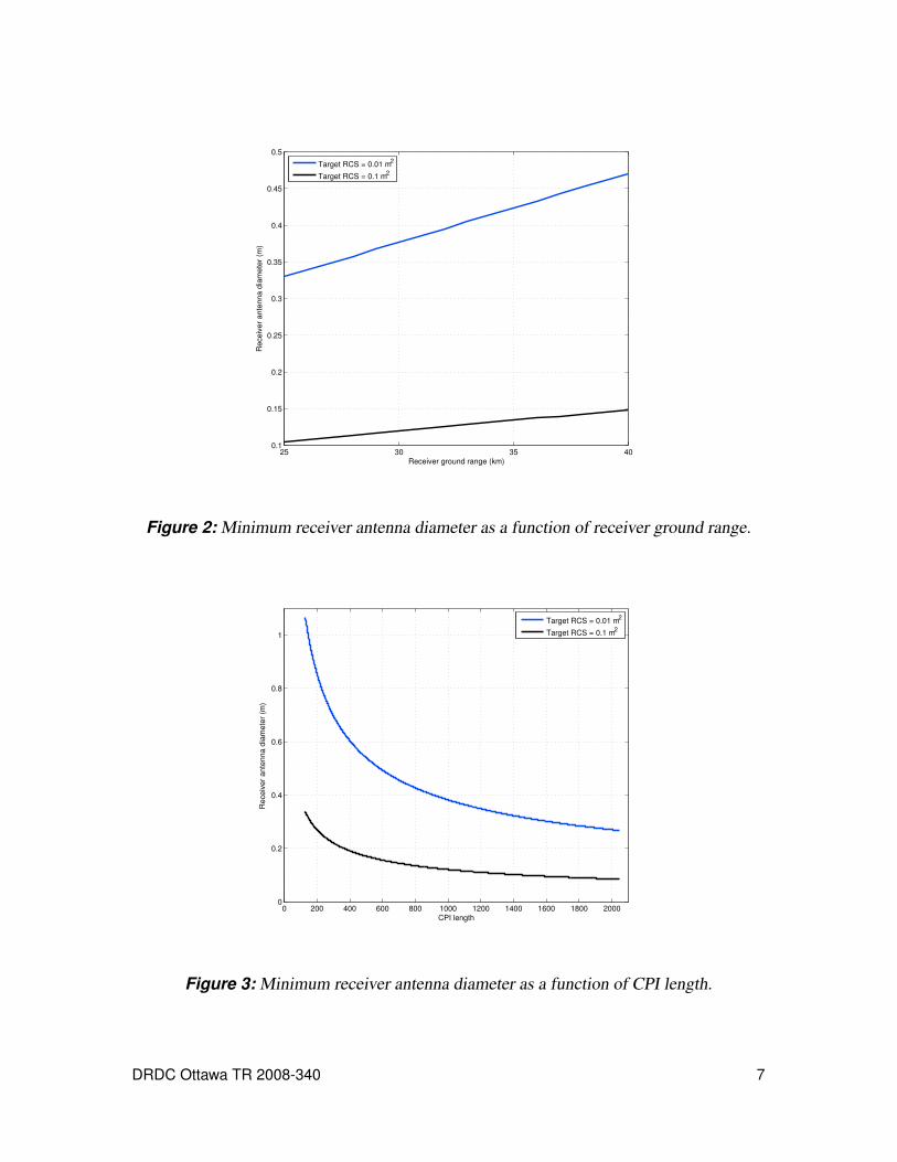
Figures 2 to 4 illustrate the trade-offs involved in selecting parameters to detect cruise
missile threats. In Figure 2 all radar parameters, except for the diameter of the receiver
antenna and receiver ground range, are held constant. The plots show the minimum receiver
diameter required as a function of receiver ground range. Since SNR is quadratic in both
receiver diameter and ground range, the plots are linear. Figure 3 shows the minimum
receiver diameter as a function of coherent processing interval (CPI) length, or NP. It is
assumed that the radar signal processor performs coherent integration in order to enhance
DRDC Ottawa TR 2008-340 5

Table 1: Radar system parameters for over-the-horizon cruise missile detection.
Parameter Definition Value
P peak power (W) 1,500
τ duty cycle 0.4
GT transmitter antenna gain
σ target RCS
Ae effective area of receiver antenna
RT transmitter-to-target range, or transmitter range
RR receiver-to-target range, or receiver range
k Boltzmann’s constant (Ws/˚K) 1.38×10⁻²³
T0 noise temperature (˚K) 290
Fn noise figure (dB) 4.3
Ls system losses (dB) 5.0
NP number of pulses 64
σ0 clutter cross-section per unit area (m2/m2)
AC area of clutter cell
PRF pulse repetition frequency (kHz) 100
SNR. Finally, Figure 4 illustrates the trade-offs between transmitter and receiver diameter,
for various values of peak power. In general there are numerous trades that can be made
among the various radar parameters. It is assumed that the radar receiver payload is larger
than that of the transmitter.
The discussion so far has focused on a single barrier. It is straightforward to extend the
concept to multiple barriers. If these barriers are all located within an azimuthal angular
extent of 120˚ then it may be possible to use a single UAV receiver above the ship, with
multiple transmitters deployed and dedicated to each barrier region. This assumes that
the receiver scans ±60˚ in azimuth. If the receiver has multiple receive channels, then
beamforming could be used to estimate the angle of arrival for each detected threat.
6 DRDC Ottawa TR 2008-340
25 30 35 400.1
0.15
0.2
0.25
0.3
0.35
0.4
0.45
0.5
Receiver ground range (km)
Re
ce
ive
r a
nte
nn
a d
iam
ete
r (m
)
Target RCS = 0.01 m2
Target RCS = 0.1 m2
Figure 2: Minimum receiver antenna diameter as a function of receiver ground range.
0 200 400 600 800 1000 1200 1400 1600 1800 20000
0.2
0.4
0.6
0.8
1
CPI length
Re
ce
ive
r a
nte
nn
a d
iam
ete
r (m
)
Target RCS = 0.01 m2
Target RCS = 0.1 m2
Figure 3: Minimum receiver antenna diameter as a function of CPI length.
DRDC Ottawa TR 2008-340 7

0 0.2 0.4 0.6 0.8 1 1.2 1.4 1.6 1.8 20
0.2
0.4
0.6
0.8
1
1.2
1.4
1.6
1.8
2
Length of receiver antenna (m)
Length
of tr
ansm
itte
r ante
nna (
m)
0.5 kW
1.0 kW
1.5 kW
2 kW
Figure 4: Required antenna dimensions for detection of a 0.01m2 target at a receiver
ground range of 30 km, for various values of peak transmitter power. Transmitter and
receiver antennas are square planar arrays.
8 DRDC Ottawa TR 2008-340
4 Sea clutter modelling and prediction
In this section, the bistatic concept is further analyzed by estimating the clutter Doppler
spectrum. Using these clutter Doppler estimates allows for the estimation of the minimum
detectable velocity (MDV). The MDV is the velocity of the slowest moving target that
can be detected by the radar. We begin by estimating the Doppler extent of sea clutter
for a bistatic radar with stationary platforms. In Subsection 4.1 the Walker model for the
Doppler spectrum of sea clutter is reviewed. This leads to predictions for the MDV of
targets in sea clutter, which are presented in Subsection 4.2.
4.1 Walker model for sea clutter Doppler spectrum
Walker has developed an analytical model for the Doppler spectrum of monostatic sea
clutter when the transmitter and receiver are stationary [10], [11]. The model is motivated
by data collected in a large wind-wave tank and by data collected from a cliff-top radar
experiment. In this model it is assumed that clutter returns are the result of components
caused by Bragg scattering, whitecap scattering, and sea spikes. Bragg scattering is caused
by reflections from smaller capillaries on the sea surface. Whitecap scattering results from
the gross movement of waves on the sea surface. Sea spikes are brief phenomena that
occur just before a wave crests. Each component of the clutter spectrum has a Gaussian
lineshape. The clutter Doppler spectrum in Hertz for vertical polarization, ΨV (v), and for
horizontal polarization, ΨH(v), are given by
ΨV (v) = BV exp
(
(v− vB)2
w2B
)
+W exp
(
(v− vG)2
w2W
)
,
ΨH(v) = BH exp
(
(v− vB)2
w2B
)
+W exp
(
(v− vG)2
w2W
)
+Sexp
(
(v− vG)2
w2S
)
,
where vB and vG are the center frequencies, wB,wW , and wS are the spectral widths, and
BV ,BH ,W,and S are the component magnitudes. In each expression the first component is
due to Bragg scattering and has a magnitude (BV or BH) that depends on polarization. The
second expression is due to whitecap scattering that is independent of polarization. For
horizontal polarization only, there is a third component caused by sea spikes.
In [11], parameters of the Walker model were matched to the Doppler distribution of X-
band sea clutter data collected by a stationary monostatic radar. For the data collection, the
radar was located at a height of 64 m above the mean sea level at a grazing angle of 3.6˚.
The radar waveform was a 500 MHz linear frequency modulation (FM) chirp centered at
9.75 GHz. The values of the Walker model parameters that matched the sea clutter data
are given in Table 2. Note that in the downwind case, the sea spike component was set to
zero in [11], because this component was absent from the measured data. Figures 5 and 6
DRDC Ottawa TR 2008-340 9

illustrate the Doppler spectra of monostatic sea clutter in upwind and downwind cases. In
the upwind case, the radar line-of-sight from the radar is the opposite of the wind direction.
In the downwind case, the radar line-of-sight from the radar is the same direction as the
wind direction.
Based on these estimates, it is reasonable to assume that in general monostatic sea clut-
ter Doppler spectra occupy the frequency band from -300 Hz to 300 Hz. Assessing the
Doppler spectrum of bistatic sea clutter is an unsolved and difficult problem. The Doppler
spectrum is likely to vary significantly with bistatic angle, sea state, and look angles from
the transmitter and from the receiver. In this study, it will be assumed that the bistatic
sea clutter Doppler spectrum also occupies the frequency band from -300 Hz to 300 Hz.
In the following analysis of minimum detectable velocity, we shall be conservative and
assume that no clutter cancellation is carried out by the radar signal processor, and that
targets whose Doppler frequencies fall within the frequency band of the clutter cannot be
detected. Moreover, we shall see that clutter cancellation is not really necessary, as targets
of interest are going to be exo-clutter if the transmitter and receiver are stationary.
Table 2: Walker model parameters for X-band radar data.
Quantity Upwind Value Downwind Value
BH/BV (dB) -15.1 -14.0
W/BH (dB) 11.5 0.2
S/BH (dB) 12.8 -
vB (Hz) 54 -15.3
vG (Hz) 178 -63.9
wB (Hz) 47.5 40.4
wW (Hz) 66.0 74.11
wS (Hz) 74.5 -
4.2 Prediction of minimum detectable velocity for
targets in sea clutter
For a bistatic radar with stationary transmitter and receiver, the Doppler shift f caused by
a moving target is given by [12]
f =2V
λcosδcos(β/2), (2)
where V is the magnitude of the target velocity vector, λ is the wavelength, β is the bistatic
angle, and δ is the angle between the target velocity vector and the bisector of the bistatic
angle. Figure 7 illustrates the geometry of a bistatic radar. From (2) the bistatic radial
10 DRDC Ottawa TR 2008-340

−500 −400 −300 −200 −100 0 100 200 300 400 5000
5
10
15
20
25
30
35
frequency (Hz)
rela
tive p
ow
er
(dB
)
V polarization
H polarization
Figure 5: Doppler spectrum of upwind sea clutter, based on Walker model.
−500 −400 −300 −200 −100 0 100 200 300 400 5000
5
10
15
20
25
30
frequency (Hz)
rela
tive p
ow
er
(dB
)
V polarization
H polarization
Figure 6: Doppler spectrum of downwind sea clutter, based on Walker model.
DRDC Ottawa TR 2008-340 11

velocity is given by V cosδcos(β/2). Note that this is a generalization of the special case
of monostatic radar, where β = 0 and δ is the angle between the radar line-of-sight and the
target velocity vector.
At X-band (10 GHz), for bistatic sea clutter with a maximum Doppler frequency of 300 Hz,
the minimum detectable velocity (MDV) is 4.5 m/s. For a bistatic radar, the radial velocity
of the target is a function of the magnitude and direction of the target’s velocity vector and
of the bistatic angle. For example, for a target with a velocity magnitude of 250 m/s, the
target is not detectable when |cosδcos(β/2)| ≤ 0.018. The values of δ and β for which this
inequality holds is shown in the area between the two black lines in Figure 8. For bistatic
angles less than 140˚, a 250 m/s target is detectable for all values of δ, except for a small
range of values near 90˚. If the locations of the transmitter and receiver are such that the
bistatic angle for all targets in the barrier is 90˚ or less, then only targets whose velocity
vectors result in a δ between 88˚ and 92˚ are not detectable. Note that targets with these
velocity vectors have a bearing of at least 45˚ away from the receiver. In other words, all
targets in the barrier that are travelling in the direction of the receiver, and thus pose the
most immediate threat to the receiver, are detected by the bistatic concept. Therefore, the
radar would not need to use clutter cancellation to detect targets under most geometries.
Figure 7: Geometry of bistatic radar, illustrating target velocity vector V, bistatic angle β,
and angle δ between velocity vector and bisector of bistatic angle.
For a transmitter and receiver that are in motion, the platform motion adds significant
spread to the clutter and increases the minimum detectable velocity. Theoretical predic-
tions for the range-Doppler spread of clutter due to platform motion have been developed
in [13]. For a transmitter and receiver each travelling with a velocity of 50 m/s, Figure
9 shows the prediction for mainlobe clutter. The blue lines show the edge of the trans-
mitter mainbeam, while the red lines show the edge of the receiver mainbeam. Due to
the high PRF waveform, there are multiple range ambiguities. Both the transmitter and
receiver mainbeams are shown, and it is assumed that the clutter will be strongest in the
areas where the mainbeams intersect. From Figure 9 it is estimated that the clutter Doppler
12 DRDC Ottawa TR 2008-340

0 20 40 60 80 100 120 140 160 1800
20
40
60
80
100
120
140
160
180
bistatic angle (deg)
delta (
deg)
Moving platforms (50 m/s)
Stationary platforms
Figure 8: Detectable geometries for bistatic concept using analytical estimates for MDV.
The area between the two black lines indicates the values of bistatic angle and δ for which
a cruise missile of velocity 250 m/s is not detectable and stationary transmitter and receiver
platforms. The two blue lines correspond to the transmitter and receiver each travelling at
a velocity of 50 m/s.
DRDC Ottawa TR 2008-340 13
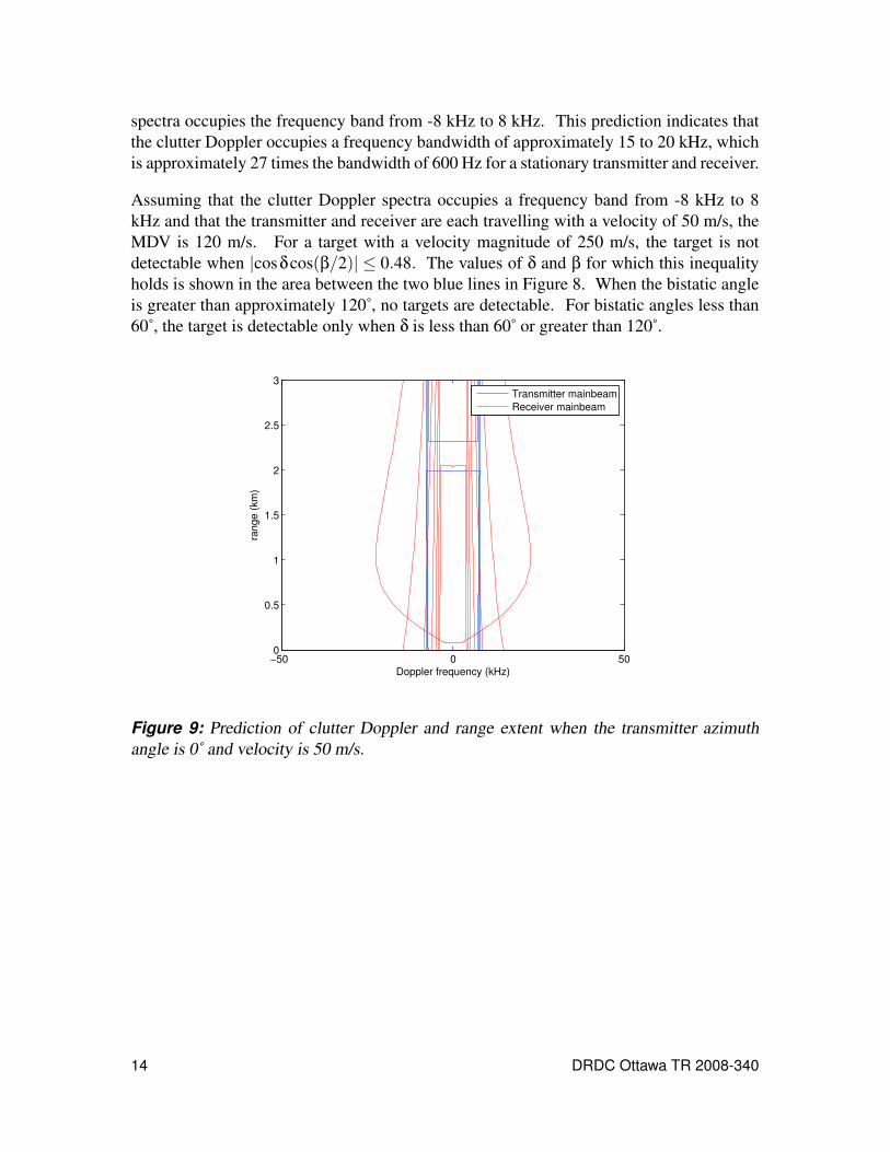
spectra occupies the frequency band from -8 kHz to 8 kHz. This prediction indicates that
the clutter Doppler occupies a frequency bandwidth of approximately 15 to 20 kHz, which
is approximately 27 times the bandwidth of 600 Hz for a stationary transmitter and receiver.
Assuming that the clutter Doppler spectra occupies a frequency band from -8 kHz to 8
kHz and that the transmitter and receiver are each travelling with a velocity of 50 m/s, the
MDV is 120 m/s. For a target with a velocity magnitude of 250 m/s, the target is not
detectable when |cosδcos(β/2)| ≤ 0.48. The values of δ and β for which this inequality
holds is shown in the area between the two blue lines in Figure 8. When the bistatic angle
is greater than approximately 120˚, no targets are detectable. For bistatic angles less than
60˚, the target is detectable only when δ is less than 60˚ or greater than 120˚.
−50 0 500
0.5
1
1.5
2
2.5
3
Doppler frequency (kHz)
range (
km
)
Transmitter mainbeam
Receiver mainbeam
Figure 9: Prediction of clutter Doppler and range extent when the transmitter azimuth
angle is 0˚ and velocity is 50 m/s.
14 DRDC Ottawa TR 2008-340
5 Simulation and Processing
The UAV radar concepts developed in this study were modelled using RLSTAP, a high-
fidelity software simulation tool developed by the Sensors Directorate at Air Force Re-
search Laboratory in Rome, NY. RLSTAP is an end-to-end simulation tool that allows for
the development and analysis of radar systems and radar signal processing algorithms. In
this study, RLSTAP was used to generate simulated radar data, and space-time adaptive
processing (STAP) algorithm development, coding and testing was done in Matlab.
5.1 RLSTAP
RLSTAP was developed under the Khoros software development environment and models
various radar system tasks and processes. Each task or process is described by software
code and is represented in the GUI as a glyph. A number of pre-defined glyphs are included
with RLSTAP, and the package allows the user to create new glyphs as well. A radar
system is simulated in RLSTAP by assembling a group of glyphs and connecting them
appropriately as a network of glyphs, also called a lineup. Because of the general nature of
the processes represented by glyphs, the simulation tool is able to simulate a wide variety of
airborne, spaceborne or ground based multi-channel radars. This allows a user to analyze
the performance of advanced radar systems and advanced signal processing techniques.
RLSTAP also allows a user to easily alter system parameters or processing techniques and
immediately see the effect of these changes on system performance.
A powerful feature of RLSTAP is its high fidelity clutter models. Realistic clutter mod-
els are vital to producing simulated data which can be used to accurately predict the per-
formance of signal processing algorithms. The software allows for the inclusion of both
clutter and jamming as interference, although in this study only clutter interference is con-
sidered. In general, the user can specify either homogeneous clutter models or realistic
clutter returns that use site-specific terrain data. Site-specific clutter is obtained from digi-
tal elevation maps (DEM’s) and land-use-land-clutter (LULC) files. See [14] for a detailed
discussion.
Figure 10 shows the RLSTAP lineup used to model a radar system. The glyph labelled
“Initialization” is an encapsulated glyph that itself represents a network of glyphs, shown
in Figure 11. The Initialization glyph establishes the details of the transmitter, receiver
and target by specifying the location, velocity, and orientation (that is, pitch, yaw and roll)
of the various platforms. Also specified in this glyph are the size, structure and antenna
patterns of the transmitter and receiver antennas. The target RCS is defined by the user in
this glyph.
In the main lineup, the “Sigma0 LUT” glyph generates a look-up table of scattering coef-
ficients as a function of grazing angle for various clutter surface types. The “Simulation
DRDC Ottawa TR 2008-340 15

Figure 10: Top level of RLSTAP workspace for UAV radar lineup.
Figure 11: Expanded view of Initialization glyph.
16 DRDC Ottawa TR 2008-340

Controller” glyph allows the user to specify various simulation parameters, such as the sim-
ulation sampling rate, minimum and maximum simulation range, and the number of pulses
per coherent processing interval. The “HomoScat” glyph specifies the clutter background
that is to be used in the simulation. The “Tx Waveform Generator” glyph generates a phase
coded transmitter waveform.
The glyph labelled “PRI Loop” is an encapsulated glyph that simulates the performance
of the physical channel and the radar receiver. Figure 12 shows the components of this
encapsulated glyph. The “Physical Model” glyph generates clutter and target returns and
performs range folding, whereby radar returns are made range ambiguous, according to the
chosen PRI. In the “Receiver Model” glyph noise is added to the waveform and filtering
is performed. The “Coherent Signal Processing” glyph then performs pulse compression
of the received waveform.
Figure 12: Expanded view of PRI Loop glyph.
The output of “PRI Loop” is a range-channel-pulse datacube. RLSTAP features a limited
number of signal processing glyphs which can be used to process datacubes. However, al-
gorithm implementation and development is more easily carried out in Matlab. As a result,
in this study, RLSTAP datacubes are exported to Matlab and processed using algorithms
written in Matlab code.
A site-specific model of the area off the coast of Maine was used in the simulation, as shown
in Figure 13. In this figure, the transmitter and transmit antenna mainbeam are represented
by the blue triangle and the blue lines. The green triangle and green lines represent the
receiver platform and receiver antenna mainbeam, respectively.
DRDC Ottawa TR 2008-340 17
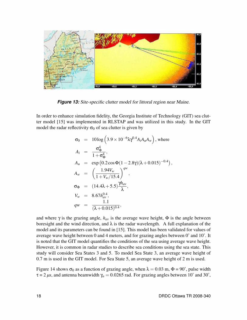
Figure 13: Site-specific clutter model for littoral region near Maine.
In order to enhance simulation fidelity, the Georgia Institute of Technology (GIT) sea clut-
ter model [15] was implemented in RLSTAP and was utilized in this study. In the GIT
model the radar reflectivity σ0 of sea clutter is given by
σ0 = 10log(
3.9×10⁻⁶λγ0.4AiAuAw
)
, where
Ai =σ4
Φ
1+σ4Φ
,
Au = exp(
0.2cosΦ(1−2.8γ)(λ+0.015)−0.4)
,
Aw =
(
1.94Vw
1+Vw/15.4
)qw
,
σΦ = (14.4λ+5.5)γhav
λ,
Vw = 8.67h0.4av ,
qw =1.1
(λ+0.015)0.4,
and where γ is the grazing angle, hav is the average wave height, Φ is the angle between
boresight and the wind direction, and λ is the radar wavelength. A full explanation of the
model and its parameters can be found in [15]. This model has been validated for values of
average wave height between 0 and 4 meters, and for grazing angles between 0˚ and 10˚. It
is noted that the GIT model quantifies the conditions of the sea using average wave height.
However, it is common in radar studies to describe sea conditions using the sea state. This
study will consider Sea States 3 and 5. To model Sea State 3, an average wave height of
0.7 m is used in the GIT model. For Sea State 5, an average wave height of 2 m is used.
Figure 14 shows σ0 as a function of grazing angle, when λ = 0.03 m, Φ = 90˚, pulse width
τ = 2 µs, and antenna beamwidth γa = 0.0265 rad. For grazing angles between 10˚ and 30˚,
18 DRDC Ottawa TR 2008-340

the values of σ0 are approximately constant and independent of grazing angle. Therefore,
it is assumed that the value of σ0 for grazing angles between 10˚ and 30˚ is the value of σ0
for a grazing angle of 10˚.
10−1
100
101
−65
−60
−55
−50
−45
−40
−35
−30
−25
Grazing angle (deg.)
σ0 (
dB
)
hav
=4 m
hav
=3 m
hav
=2 m
hav
=1 m
Figure 14: σ0 as a function of grazing angle, when λ = 0.03m, Φ=90˚, τ = 2µs, and
γa = 0.0265 rad.
5.2 Space-Time Adaptive Processing
In this section we discuss space-time adaptive processing (STAP) of the output data from
the ‘PRI Loop’ glyph. This data has been down converted, matched filtered and pulse
compressed, assuming a 13-bit Barker code on the transmitted waveform. As a result,
the output of the ‘PRI Loop’ glyph is a three-dimensional data cube of complex samples
which are indexed by range, channel, and pulse. Consider M pulses, N channels, and a
fixed range gate. Define the MN-dimensional data vector x, where
x =
x0
x1...
xM−1
, (3)
and each xi is a N-dimensional vector of returns from N channels for pulse i. A STAP pro-
cessor takes the data vector x as input and considers whether a target is present at Doppler
frequency fd . The output is a (scalar) test statistic z, which is passed to a threshold detector.
The threshold detector compares z to a threshold and makes a target detection decision.
DRDC Ottawa TR 2008-340 19

Let the data vector be given by (3). STAP constructs an MN-dimensional linear filter w
and computes the test statistic z = w · x. The data vector x can be factored as the sum of
the returns due to signal and interference. That is, x = xt +xI , where xt is the signal return
and xI is the interference and noise return that may include clutter, receiver noise and noise
jamming. STAP computes the linear filter that maximizes the signal-to-interference-plus-
noise ratio (SINR) of the filtered data vector. The optimal STAP filter is
w = argmaxy
|y · xt ||y · xI|
, (4)
that is, w is the vector that maximizes the quotient|y·xt ||y·xI | over all choices of y.
For the case of homogeneous interference with a known covariance matrix R = E[xIx∗I ], it
was shown [16] that the optimal filter is given by
w = R−1s, (5)
where s is the target steering vector. The target steering vector is defined to be the MN-
dimensional vector with the same phase as the expected return from the target only, but with
normalized magnitude. It will be assumed that (5) is optimal, even when the interference is
not homogeneous. In realistic environments, R is not known and must be estimated. In this
study, R is estimated by using a secondary data set (SDS) in nearby range cells. Sample
matrix inversion (SMI) then estimates R−1 by taking the inverse of the sample matrix.
Fully Adaptive STAP processes an NM-dimensional data vector, consisting of returns from
all N channels and all M pulses. For even moderate values of N and M, Fully Adaptive
STAP is too computationally intensive for real-time applications. Furthermore higher di-
mensions of R require larger SDSs to provide good covariance estimates. However, in non-
homogeneous environments, interference characteristics can vary widely throughout larger
SDSs. This motivates the search for reduced dimension methods, where one processes
fewer pulses and channels simultaneously. These methods are called partially adaptive
STAP methods, require less processing complexity and allow for the use of smaller SDSs.
Partially adaptive STAP is much more amenable to real-time applications. These methods
process data from less than N channels and/or less than M pulse returns at a time. As a re-
sult, the inverses of much smaller dimension matrices need to be computed. Furthermore,
the secondary data sets used for covariance estimation can be smaller, which is advanta-
geous in non-homogeneous interference environments. We now give a brief outline of the
partially adaptive STAP methods used in this study, Adapt-then-filter STAP and Factored
STAP.
Adapt-then-filter STAP (also called element space pre-Doppler STAP in [17]) performs
adaptive filtering of a small number of pulses, K, followed by Doppler filtering. Adapt-
then-filter STAP operates in a sliding window fashion. Specifically, Adapt-then-filter STAP
forms K-dimensional data sub-vectors
20 DRDC Ottawa TR 2008-340

xAT F,i =
xi
xi+1...
xi+K−1
, i = 0, ...,M−K. (6)
For each i, the weight vector wAT F,i = R−1AT F,i sAT F,i is computed, where RAT F,i is an estimate
of the covariance matrix of xAT F,i, and sAT F,i is a MK-dimensional steering vector, defined
as u⊗sS, where sS is the spatial steering vector and u is a K-dimensional binomial taper. For
sub-vector i, the adaptive output is yAT F,i = wAT F,i · xAT F,i. A test statistic zAT F is computed
as zAT F = f · yAT F , where yAT F = [yAT F,0 yAT F,1 ... yAT F,M−K]T and f is a Doppler filter of
length M −K + 1 corresponding to the first M −K + 1 elements of the time-only steering
vector sT .
Factored STAP (also called Post-Doppler adaptive beamforming in [17]) performs Doppler
filtering on each channel followed by adaptive filtering of all channels in each Doppler bin.
Let y1,y2, · · · ,yN be the M-dimensional data vectors for each of the N channels. Consider
Doppler bin i, and let fi be the corresponding Doppler filter of length M. The Post-Doppler
data set is given by
xF,i = [ fi · y1 fi · y2 · · · fi · yN ]T . (7)
For Doppler bin i, Post-Doppler STAP computes the weight vector wF,i = R−1F,i sF,i, where
RF,i is an estimate of the covariance matrix of xF,i, and sF,i is the pot-Doppler target spatial
steering vector. The test statistic for Doppler bin i is then given by zF,i = wF,i · xF,i.
The performance of the STAP techniques will be measured by computing the improvement
factor, which is the ratio of the SINR after processing to the SINR before processing. As
will be seen in the IF plots, the IF typically is lower for target Doppler frequencies in the
clutter notch, where the clutter Doppler power is strongest. The value of the improvement
factor near the clutter notch measures the extent to which STAP cancels clutter power while
preserving target power. The improvement factor outside of the clutter notch indicates the
ability of STAP to detect targets in noise.
STAP performance will also be measured by computing MDV and usable Doppler space
fraction (UDSF). The usable Doppler space fraction is the fraction of the Doppler space
over which a target can be detected. The MDV is determined by estimating the clutter
power after STAP processing.
DRDC Ottawa TR 2008-340 21
6 Concept Performance
As discussed earlier, the UAV radar system is designed to provide a barrier search detection
capability. The barrier is assumed to be a rectangular region near the Earth’s surface, with
dimensions 14 km by 5 km. It is assumed that the barrier is located 25 km to 30 km
from the ship. The goal of the UAV system is to detect all cruise missile targets that cross
through the barrier. In this section the performance of the bistatic radar system is evaluated
by simulating radar scenarios in RLSTAP. Three different scenarios are considered. A ship
self-defence scenario is simulated in Subsection 6.1, and area air defence scenarios are
simulated in Subsections 6.2 and 6.3.
In order to assess UAV radar performance, a specific missile trajectory within the barrier
is assumed. For the entire trajectory, the missile is assumed to be travelling at an altitude
of 10 m with a velocity of 250 m/s. The missile trajectory has three distinct segments, as
shown in Figure 15. In the first segment, the missile travels for a distance of 2.8 km at a
45˚ angle to the long axis of the barrier. During the second segment, a distance of 5.1 km is
travelled on a straight line that is almost parallel to the long axis of the barrier. In the third
and final segment, the missile travels for a distance of 2 km on a course that is parallel to the
short axis of the barrier. The segments of the trajectory are designed to provide differing
geometries in the simulation results.
For the RLSTAP simulations, the transmit antenna is a 0.4 m-by-0.4 m side-looking, rect-
angular array. The transmitted waveform has a PRF of 100 kW with a pulse width of 3.9
µs. The high PRF waveform was chosen so that the velocity of a Mach 2 target could be re-
solved unambiguously. Coherent pulse intervals of 64 pulses are transmitted, and the peak
transmitted power is 1.5 kW. The receive antenna is a 1 m-by-3 m side-looking, rectangular
array with 3 sub-apertures and 0.4 m spacing between sub-apertures.
6.1 Ship Self-Defence
The barrier may be specified at any orientation with respect to the ship. To model a ship
self-defence scenario, the barrier is aligned as shown in Figure 16. The transmitter flies in
a racetrack near the barrier, while the receiver flies in a racetrack above the ship. Both the
transmitter and receiver antennas scan the barrier to search for targets. Note that multiple
transmitter and receiver platforms would be required to provide persistent coverage of the
barrier. That is, if it is assumed that the transmitter antenna looks to one side only, then a
single UAV can only provide barrier coverage for one leg of the racetrack. Two or more
transmitter UAVs could be used to provide persistent coverage. Similarly, if the receiver
antenna looks to one side only, multiple UAVs would be required to provide persistent
coverage.
The performance of the proposed bistatic UAV radar is evaluated by simulating the radar re-
22 DRDC Ottawa TR 2008-340

Figure 15: Top-down view of missile trajectory through rectangular detection barrier.
Figure 16: Top-down view of UAV radar configuration for ship self-defence.
DRDC Ottawa TR 2008-340 23

turns when the cruise missile target is halfway through each segment in its trajectory. That
is, there were three separate simulation scenarios run for the ship self-defence configura-
tion. These are summarized in Table 3. The points in the missile trajectory corresponding
to Scenarios A, B and C are shown in Figure 16.
Table 3: Simulation scenarios for ship self-defence configuration.
Target Bistatic Bistatic Bistatic
Scenario Segment Range (km) Doppler (kHz) Angle (˚)
A 1 39.1 13.5 16.5
B 2 35.1 4.6 8.8
C 3 32.0 16.7 8.0
In this configuration, the transmitter and receiver are aligned so that the bistatic angle is
generally close to zero. Thus, as is the case with monostatic radar, crossing targets with
small radial velocity can be buried in the clutter and are difficult to detect. However, these
targets are less of a threat to the ship, because they are not headed in the direction of
the ship. Higher velocity missiles pose a bigger threat because they decrease the radar’s
reaction time, but higher velocity crossing missiles have greater Doppler frequency and are
easier to detect than lower velocity missiles.
Scenario A was simulated in RLSTAP, with an illustration of the geometry shown in Fig-
ure 13. In order to produce a sea clutter background, the radar system was oriented so that
the radar footprints contained only sea clutter. To produce a littoral clutter background, the
system was oriented so that land clutter and sea clutter were contained in the radar foot-
prints. For Scenario A with a littoral clutter background and sea state 3 for the sea clutter,
the range-Doppler map shown in Figure 17. It is seen that the target return is located at
the expected bistatic range of 39.1 km, with a bistatic Doppler of 13.5 kHz. Although
the target return is much weaker than that of the clutter return, the target can be detected
because it is outside of the clutter Doppler space. The Doppler processing separates the
clutter and target in Doppler and allows the target to be detected, since the target is above
the noise floor. Figure 18 shows the Doppler magnitude at the range where target response
is strongest. Figure 19 shows the improvement factors for STAP processing. For both tech-
niques, the IF is higher for larger frequencies that are outside the clutter Doppler. At zero
Doppler, where the clutter is strongest, the IF decreases by about 30 dB. This decrease in
IF is also called the clutter notch. The Adapt-then-filter technique has better performance
than Factored STAP, especially at the smaller positive frequencies near the clutter notch.
Note that both STAP techniques have IFs that are 30 dB greater than that of Doppler pro-
cessing. This gain is due to the adaptivity that is used in Adapt-then-filter and Factored
STAP. For Doppler processing, the minimum detectable velocity is 70.3 m/s, correspond-
ing to a Doppler frequency of 4.7 kHz. For both STAP techniques, the MDV is 46.9 m/s,
corresponding to a Doppler frequency of 3.1 kHz.
24 DRDC Ottawa TR 2008-340

Figure 19 shows STAP performance for Scenario A for littoral clutter and sea state 3.
Scenario A was also simulated for sea clutter and sea state 5. Figure 20 shows the resulting
STAP performance. In this case, ATF has better performance at all Doppler frequencies.
Furthermore, the gain in STAP performance compared to Doppler processing is 10 dB
greater than for a littoral background with sea state 3.
Under Scenario A, two different clutter types were considered, sea clutter and littoral clut-
ter. As well, two different sea states were considered, sea states 3 and 5. For all four
possible clutter backgrounds, simulations were run in RLSTAP, with results processed us-
ing STAP. Figure 21 shows the results for Adapt-then-filter processing. It is evident that
the IF is larger for the sea clutter backgrounds than for the littoral backgrounds. The littoral
background is a mixture of land and sea clutter, and the heterogeneity of the clutter results
in poorer performance compared to homogeneous sea clutter in this case. For sea clutter,
Figure 21 also indicates that changing the sea state from 3 to 5 augments the IF by 3 to 5
dB for most of the Doppler spectrum. For the littoral background, changing the sea state
has almost no effect on performance.
Figure 22 compares the performance of Factored STAP for all four clutter backgrounds.
Over most of the Doppler spectrum, Factored STAP has higher IF for sea clutter compared
to littoral clutter. For sea clutter, the performance for sea state 3 and sea state 5 is very
closely matched. However, for littoral clutter, performance is 5 to 10 dB better for sea state
3 than for sea state 5. Note that all four clutter backgrounds result in the same performance
in the clutter notch.
For Scenario B, which corresponds to the second segment of the missile trajectory, the
range-Doppler plot is shown in Figure 23. During the second segment, the missile is al-
most a crossing target relative to both the transmitter and the receiver. As a result, the
target has very little radial velocity and is partly obscured by the clutter Doppler. Figure 24
shows the improvement factors for Scenario B. Adapt-then-filter processing has better per-
formance than Factored STAP. The increase in performance of STAP processing compared
to Doppler processing is similar to that from Scenario A.
In Scenario C, the target is in the third segment of its trajectory and is heading directly
towards the ship. As a result, the target is outside of the clutter Doppler space and can be
detected without STAP processing. Figure 25 shows IFs for STAP and Doppler process-
ing for Scenario C. As was the case with Scenarios A and B, Adapt-then-filter has better
performance than Factored STAP.
Recall that Figure 8 used an analytical estimate for the Doppler extent of sea clutter to
determine the detectable geometries for specified transmitter, receiver and target velocities.
This plot showed the values for δ and β for which the resulting bistatic Doppler frequency
was greater than that of the clutter Doppler. Using the MDV values for Scenarios A, B and
C, it is evident that the Doppler extent of clutter is from -4.7 kHz to 4.7 kHz for Doppler
processing and from -3.1 kHz to 3.1 kHz for STAP processing. Figure 26 presents the
DRDC Ottawa TR 2008-340 25

detectable geometries for a transmitter and receiver with a velocity of 50 m/s and a target
with a velocity of 250 m/s, using the values of MDV that were generated from simulations.
The results are slightly different that those in Figure 8, which shows the detectable geome-
tries for an analytical estimate of MDV. For the ship self-defence configuration, the bistatic
angle varies between 0˚ and 60˚. It is evident that after STAP processing a target can be
detected as long as δ is less than 80˚ or greater than 100˚.
Doppler (Hz)
Range (
km
)
−5 −4 −3 −2 −1 0 1 2 3 4
x 104
37.5
38
38.5
39
39.5
40
−8
−7
−6
−5
−4
−3
Figure 17: Range-Doppler map of returns from Scenario A with littoral background and
Sea State 3.
26 DRDC Ottawa TR 2008-340
−5 −4 −3 −2 −1 0 1 2 3 4 5
x 104
10−8
10−7
10−6
10−5
10−4
10−3
10−2
Doppler (Hz)
Am
plit
ude
Figure 18: Range cross-cut showing Doppler magnitude of clutter and target response for
Scenario A with littoral background and Sea State 3.
−5 0 5
x 104
0
10
20
30
40
50
60
70
80
90
100
Doppler frequency (Hz)
Impro
vem
ent F
acto
r (d
B)
Doppler processing
Adapt−then−filter
Factored STAP
Figure 19: STAP improvement factors for Scenario A with littoral background and Sea
State 3.
DRDC Ottawa TR 2008-340 27

−5 0 5
x 104
10
20
30
40
50
60
70
80
90
100
110
Doppler frequency (Hz)
Impro
vem
ent F
acto
r (d
B)
Doppler processing
Adapt−then−filter
Factored STAP
Figure 20: STAP improvement factors for Scenario A with sea clutter background and Sea
State 5.
−5 0 5
x 104
30
40
50
60
70
80
90
100
110
Doppler frequency (Hz)
Impro
vem
ent F
acto
r (d
B)
Sea clutter, sea state 3
Littoral, sea state 3
Sea clutter, sea state 5
Littoral, sea state 5
Figure 21: Comparison of Adapt-then-filter improvement factors for various clutter back-
grounds for Scenario A.
28 DRDC Ottawa TR 2008-340

−5 0 5
x 104
40
50
60
70
80
90
100
Doppler frequency (Hz)
Impro
vem
ent F
acto
r (d
B)
Sea clutter, sea state 3
Littoral, sea state 3
Sea clutter, sea state 5
Littoral, sea state 5
Figure 22: Comparison of Factored STAP improvement factors for various clutter back-
grounds for Scenario A.
Doppler (Hz)
Ra
ng
e (
km
)
−4 −2 0 2 4
x 104
34.5
35
35.5
36
36.5
37
−9
−8
−7
−6
−5
−4
−3
−2
Target
Figure 23: Range-Doppler map of radar returns from Scenario B with littoral background
and Sea State 3.
DRDC Ottawa TR 2008-340 29

−5 0 5
x 104
0
10
20
30
40
50
60
70
80
Doppler frequency (Hz)
Impro
vem
ent F
acto
r (d
B)
Doppler processing
Adapt−then−filter
Factored STAP
Figure 24: STAP improvement factors for Scenario B with littoral background and Sea
State 3.
−5 0 5
x 104
0
10
20
30
40
50
60
70
80
Doppler frequency (Hz)
Impro
vem
ent F
acto
r (d
B)
Doppler processing
Adapt−then−filter
Factored STAP
Figure 25: STAP improvement factors for Scenario C with littoral background and Sea
State 3.
30 DRDC Ottawa TR 2008-340

0 20 40 60 80 100 120 140 160 1800
20
40
60
80
100
120
140
160
180
bistatic angle (deg)
delta (
deg)
Doppler processing
STAP
Figure 26: Detectable geometries for bistatic concept using MDV derived from simula-
tions. The transmitter and receiver have velocities of 50 m/s and the target has a velocity of
250 m/s. For a given bistatic angle, the target cannot be detected if its δ angle is between
the two lines.
6.2 Area Air Defence, Configuration 1
In the previous subsection, the UAV radar was used to provide ship self-defence. The
UAV radar may also be used to provide area air-defence. Figure 27 illustrates an area air
defence scenario, where Ship A is tasked with defending ship B. In this case, the radar again
attempts to detect cruise missiles that pass through a rectangular barrier in the direction of
Ship B. The barrier is beyond Ship A’s horizon and may or may not be beyond Ship B’s
horizon. This configuration is the first area air-defence configuration considered in this
report. A second configuration is considered in the next subsection.
Table 4: Simulation scenarios for area air defence, configuration 1.
Target Bistatic Bistatic Bistatic
Scenario Segment Range (km) Doppler (kHz) Angle (˚)
D 1 35.5 8.5 56.2
E 2 34.2 -1.3 48.6
F 3 33.2 14.4 39.0
Three scenarios were simulated in RLSTAP, with each scenario corresponding to the mid-
point of a target segment. Table 4 lists the scenarios and the resulting bistatic range and
DRDC Ottawa TR 2008-340 31
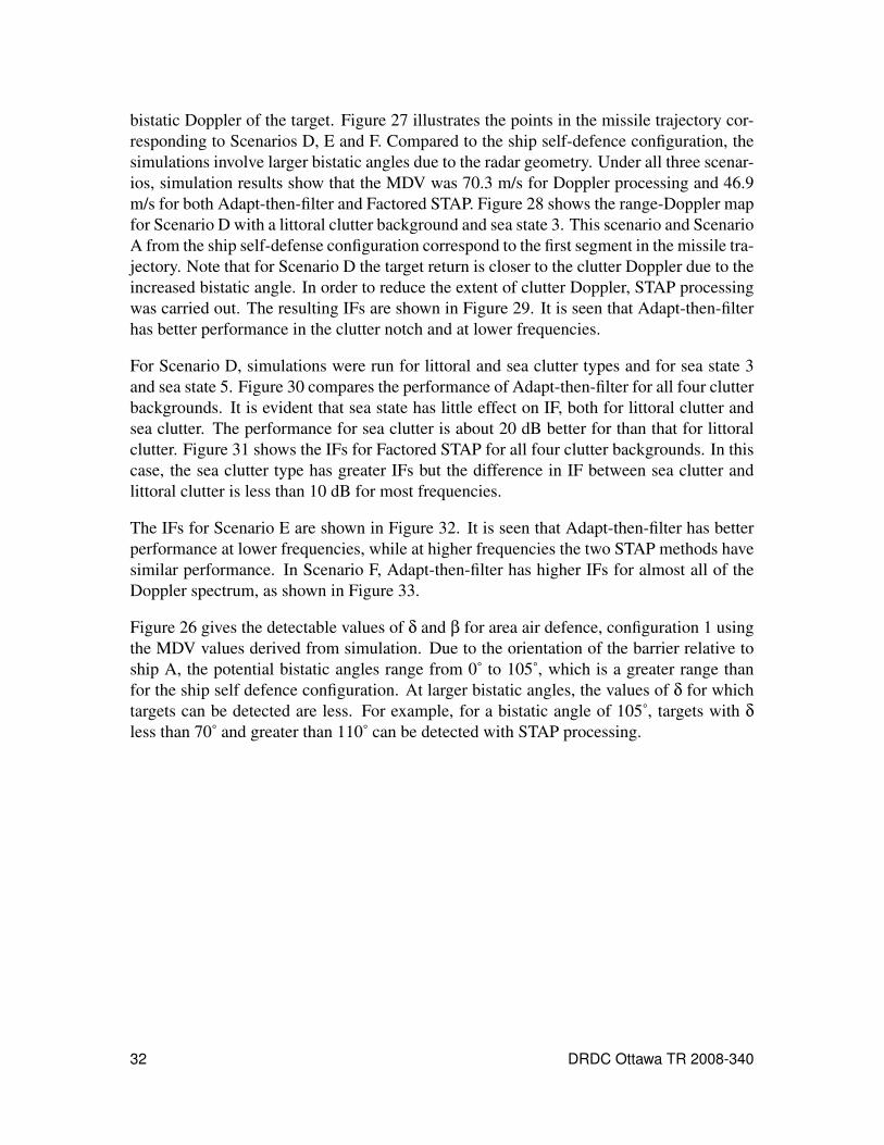
bistatic Doppler of the target. Figure 27 illustrates the points in the missile trajectory cor-
responding to Scenarios D, E and F. Compared to the ship self-defence configuration, the
simulations involve larger bistatic angles due to the radar geometry. Under all three scenar-
ios, simulation results show that the MDV was 70.3 m/s for Doppler processing and 46.9
m/s for both Adapt-then-filter and Factored STAP. Figure 28 shows the range-Doppler map
for Scenario D with a littoral clutter background and sea state 3. This scenario and Scenario
A from the ship self-defense configuration correspond to the first segment in the missile tra-
jectory. Note that for Scenario D the target return is closer to the clutter Doppler due to the
increased bistatic angle. In order to reduce the extent of clutter Doppler, STAP processing
was carried out. The resulting IFs are shown in Figure 29. It is seen that Adapt-then-filter
has better performance in the clutter notch and at lower frequencies.
For Scenario D, simulations were run for littoral and sea clutter types and for sea state 3
and sea state 5. Figure 30 compares the performance of Adapt-then-filter for all four clutter
backgrounds. It is evident that sea state has little effect on IF, both for littoral clutter and
sea clutter. The performance for sea clutter is about 20 dB better for than that for littoral
clutter. Figure 31 shows the IFs for Factored STAP for all four clutter backgrounds. In this
case, the sea clutter type has greater IFs but the difference in IF between sea clutter and
littoral clutter is less than 10 dB for most frequencies.
The IFs for Scenario E are shown in Figure 32. It is seen that Adapt-then-filter has better
performance at lower frequencies, while at higher frequencies the two STAP methods have
similar performance. In Scenario F, Adapt-then-filter has higher IFs for almost all of the
Doppler spectrum, as shown in Figure 33.
Figure 26 gives the detectable values of δ and β for area air defence, configuration 1 using
the MDV values derived from simulation. Due to the orientation of the barrier relative to
ship A, the potential bistatic angles range from 0˚ to 105˚, which is a greater range than
for the ship self defence configuration. At larger bistatic angles, the values of δ for which
targets can be detected are less. For example, for a bistatic angle of 105˚, targets with δ
less than 70˚ and greater than 110˚ can be detected with STAP processing.
32 DRDC Ottawa TR 2008-340

Figure 27: Top-down view of area air defence, configuration 1.
Doppler (Hz)
Ra
ng
e (
km
)
−4 −2 0 2 4
x 104
34.5
35
35.5
36
36.5
37
−10
−9
−8
−7
−6
−5
−4
−3
Figure 28: Range-Doppler map of returns from Scenario D with littoral background and
Sea State 3.
DRDC Ottawa TR 2008-340 33

−5 0 5
x 104
0
10
20
30
40
50
60
70
80
90
100
Doppler frequency (Hz)
Impro
vem
ent F
acto
r (d
B)
Doppler processing
Adapt−then−filter
Factored STAP
Figure 29: STAP improvement factors for Scenario D with littoral background and Sea
State 3.
−5 0 5
x 104
40
50
60
70
80
90
100
110
120
130
Doppler frequency (Hz)
Impro
vem
ent F
acto
r (d
B)
Sea clutter, sea state 3
Littoral, sea state 3
Sea clutter, sea state 5
Littoral, sea state 5
Figure 30: Comparison of Adapt-then-filter improvement factors for various clutter back-
grounds for Scenario D.
34 DRDC Ottawa TR 2008-340

−5 0 5
x 104
30
40
50
60
70
80
90
Doppler frequency (Hz)
Impro
vem
ent F
acto
r (d
B)
Sea clutter, sea state 3
Littoral, sea state 3
Sea clutter, sea state 5
Littoral, sea state 5
Figure 31: Comparison of Factored STAP improvement factors for various clutter back-
grounds for Scenario D.
−5 0 5
x 104
0
10
20
30
40
50
60
70
80
90
Doppler frequency (Hz)
Impro
vem
ent F
acto
r (d
B)
Doppler processing
Adapt−then−filter
Factored STAP
Figure 32: STAP improvement factors for Scenario E with littoral background and Sea
State 3.
DRDC Ottawa TR 2008-340 35

−5 0 5
x 104
0
10
20
30
40
50
60
70
80
90
100
Doppler frequency (Hz)
Impro
vem
ent F
acto
r (d
B)
Doppler processing
Adapt−then−filter
Factored STAP
Figure 33: STAP improvement factors for Scenario F with littoral background and Sea
State 3.
6.3 Area Air Defence, Configuration 2
A second area air-defence configuration was studied, as represented by Figure 34. Once
again, the UAV radar augments the sensor capability of ship A, in order to detect threats
to ship B. Because of the geometry of this configuration, the range of bistatic angles are
greater than that for the first area air defence configuration. Table 5 shows the scenarios and
resulting bistatic range and Doppler for this configuration, where each scenario corresponds
to the midpoint of the target segment, as shown in Figure 34. Under all three scenarios,
the MDV is 70.3 m/s for Doppler processing and 46.9 m/s for both Adapt-then-filter and
Factored STAP.
Table 5: Simulation scenarios for area air defence, configuration 2.
Target Bistatic Bistatic Bistatic
Scenario Segment Range (km) Doppler (kHz) Angle (˚)
G 1 31.2 2.1 102.8
H 2 32.3 -5.4 91.8
I 3 33.1 8.9 79.7
Figure 35 shows the range-Doppler map for radar returns from Scenario G. The target
return is buried in the clutter return, and as a result cannot be seen in the figure. This
contrasts with Scenario A and Scenario D from the ship self-defence configuration and
36 DRDC Ottawa TR 2008-340

area air-defence, configuration 1, respectively. In those configurations, the bistatic angle
and velocity vector of the target are such that the target appears outside of the clutter. In
this case, the bistatic angle is larger, and the relative direction of the velocity vector is such
that the bistatic radial velocity is small. The improvement factors for STAP are shown in
Figure 35. It is seen that Adapt-then-filter has larger IF for most of the Doppler spectrum
and especially near the clutter notch.
Scenario G was simulated for sea clutter and littoral clutter types, and for sea state 3 and
sea state 5. Figure 37 compares the performance of Adapt-then-filter for all four clutter
backgrounds. The IFs for the sea clutter backgrounds are greater than those for the littoral
backgrounds. For Factored STAP, shown in Figure 38, the littoral backgrounds have lower
IFs compared to those for the sea clutter backgrounds.
In Scenario H, the target is almost a crossing target relative to ship B, but because of the
bistatic geometry, it has large Doppler relative to ship A. As a result, the bistatic Doppler is
large enough that it is located outside of the clutter. Figure 39 shows that Adapt-then-filter
has higher IFs than Factored STAP for this scenario. The cruise missile is heading directly
toward ship B under Scenario I, and the Doppler response of the target is outside that of
the mainlobe clutter. In Figure 40, it is seen that Adapt-then-filter and Factored STAP have
similar performance throughout most of the Doppler spectrum.
When considering detectable geometries, the relationship between δ and β is shown in
Figure 26. Due to the orientation of the barrier relative to ship A, the potential bistatic angle
ranges from 30˚ to 150˚. As bistatic angle increases, the values of δ for which the target is
detectable decrease. Because of the barrier orientation in area air defence, configuration 2,
the target Doppler response for Scenario G is buried in the clutter Doppler. For Scenarios
A and D, the bistatic angle is smaller and the targets are detectable.
6.4 Discussion
The simulation results presented in this section indicate a number of interesting conclu-
sions. There are a number of results that are common to the ship self-defence and both
area air defence configurations. For all three configurations, STAP processing has higher
improvement factors than Doppler processing. In addition, Adapt-then-filter has higher IFs
than Factored STAP in most cases. For all scenarios, the MDV is 70.3 m/s for Doppler
processing and 46.9 m/s for both Adapt-then-filter and Factored STAP. The consistency of
the MDV values is likely due to the high PRF waveform, which results in the clutter power
being concentrated in a limited number of Doppler cells near zero frequency.
The different geometries associated with the three configurations have a significant effect
on the detectability of targets. For the ship self-defence configuration, a target is not de-
tectable if it has low radial velocity in the direction of the ship. For the area air defence
DRDC Ottawa TR 2008-340 37

configurations, the bistatic angle is larger. As a result it is possible for some crossing tar-
gets to be detected, while other targets that are heading more directly toward the ship may
not be detected. The design of an area air defence configuration will have to be carefully
considered to account for this effect.
Figure 34: Top-down view of area air defence, configuration 2.
38 DRDC Ottawa TR 2008-340

Doppler (Hz)
Ra
ng
e (
km
)
−4 −2 0 2 4
x 104
28.5
29
29.5
30
30.5
31
−9
−8
−7
−6
−5
−4
−3
Target
Figure 35: Range-Doppler map of returns from Scenario G with littoral background and
Sea State 3.
−5 0 5
x 104
0
10
20
30
40
50
60
70
80
90
Doppler frequency (Hz)
Impro
vem
ent F
acto
r (d
B)
Doppler processing
Adapt−then−filter
Factored STAP
Figure 36: STAP improvement factors for Scenario G with littoral background and Sea
State 3.
DRDC Ottawa TR 2008-340 39

−5 0 5
x 104
40
50
60
70
80
90
100
110
Doppler frequency (Hz)
Impro
vem
ent F
acto
r (d
B)
Sea clutter, sea state 3
Littoral, sea state 3
Sea clutter, sea state 5
Littoral, sea state 5
Figure 37: Comparison of Adapt-then-filter improvement factors for various clutter back-
grounds for Scenario G.
−5 0 5
x 104
40
45
50
55
60
65
70
75
80
85
90
Doppler frequency (Hz)
Impro
vem
ent F
acto
r (d
B)
Sea clutter, sea state 3
Littoral, sea state 3
Sea clutter, sea state 5
Littoral, sea state 5
Figure 38: Comparison of Factored STAP improvement factors for various clutter back-
grounds for Scenario G.
40 DRDC Ottawa TR 2008-340

−5 0 5
x 104
0
10
20
30
40
50
60
70
80
90
Doppler frequency (Hz)
Impro
vem
ent F
acto
r (d
B)
Doppler processing
Adapt−then−filter
Factored STAP
Figure 39: STAP improvement factors for Scenario H with littoral background and Sea
State 3.
−5 0 5
x 104
0
10
20
30
40
50
60
70
80
90
100
110
Doppler frequency (Hz)
Impro
vem
ent F
acto
r (d
B)
Doppler processing
Adapt−then−filter
Factored STAP
Figure 40: STAP improvement factors for Scenario I with littoral background and Sea
State 3.
DRDC Ottawa TR 2008-340 41

7 Small Boat Radar Cross Section
The remainder of this report will focus on the problem of small boat detection using UAV
radar. The Maritime Force Protection (MFP) Technology Demonstration Project (TDP)
is studying force protection against the small boat threat. One component of the TDP is
examining the use of UAVs to detect small boats. DRDC Ottawa is supporting this effort
by studying radar detection using UAVs.
The “Legend” small boat, shown in Figure 41, is being used in live weapons experiments
under the MFP TDP. This boat is considered the main threat in designing a UAV radar
system to detect small boat threats. A key step in predicting radar system performance
involves the prediction of the RCS of the small boat. Such predictions of the monostatic
and bistatic RCS are presented in this section.
Figure 41: The Legend small boat and CAD model.
A CAD model of the Legend was produced and is shown in Figure 41. This document
considers a monostatic UAV concept, and the monostatic RCS measurements are relevant
to the analysis. Future work may consider the use of bistatic UAV concepts. In this case
bistatic RCS measurements would be required to carry out an analysis. The bistatic RCS
results are provided here for completeness.
The software Rapport was used to model the electromagnetic signature of the Legend
model. The RCS σ of an object is given by
σ = limR→∞
4πR2
∣
∣
∣
∣
EscatteredEincident
∣
∣
∣
∣
2
, (8)
where Eincident is the incident field strength, Escattered is the scattered field strength, and
R is the distance from the object to the location where field strength is measured. In this
modelling, the material of the boat is specified as a perfect conductor. Rapport uses a
“shooting and bouncing” ray technique to compute the scattered field strength. Specifi-
cally, a set of parallel rays are launched from the incident direction. Each ray is traced
as it bounces from one part of the object to another until it exits the object. To compute
the effect of the first bounce, Physical Optics is used, while subsequent bounces use the
42 DRDC Ottawa TR 2008-340

Physical Theory of Diffraction. The radar frequency used is 10.0 GHz (X-band) with
VV polarization. It is assumed that the boat is located in the open ocean in Sea State 1.
The RCS measurements predicted include the direct path and multi-path reflections. The
multi-path reflections include boat-to-sea, sea-to-boat, and sea-to-boat-to-sea.
The RCS of the Legend model is predicted for a variety of transmitter and receiver posi-
tions. As shown in Figure 42, the center of the boat is placed at the origin of a three-
dimensional coordinate system. Without loss of generality, it is assumed that the primary
axis of the boat body is aligned with the x-axis. The locations of the transmitter and re-
ceiver are given in spherical coordinates, where angles θi and φi specify the transmitter
position, while θr and φr specify that of the receiver. The angles θi and θr are varied be-
tween 5˚ and 90˚ degrees, while φi and φr are varied between 0˚ and 360˚. It is noted that
the transmitter range and receiver range need not be considered, because the RCS does not
depend on the ranges from the transmitter and receiver, assuming that the target is in the
far-field of both the transmitter and receiver.
To begin the experiment, the transmitter is placed at a fixed location. The receiver is then
placed at various locations around the boat, in spherical coordinates with 5˚ increments in
θr and φr. The RCS is computed for each receiver position. Therefore, for each fixed
transmitter position, there are 1,314 receiver positions, at each of which an RCS measure-
ment is predicted. The transmitter is positioned at various locations around the boat, with
30˚ increments in θi and φi.
Figure 42: Coordinate system for bistatic RCS modelling.
Table 6 shows the modelled monostatic RCS for a number of transmitter positions. There
DRDC Ottawa TR 2008-340 43

is a large variation in RCS as the elevation angle θi varies. The RCS is largest when θi=60˚.
This large RCS value appears to be caused by a strong reflection from the bench seats. In
Annex A, a full analysis of the monostatic and bistatic RCS is presented. It is shown that 0
dBsm is the median monostatic RCS of the Legend small boat. This value for RCS will be
used in the following sections. Although bistatic radar is not considered in this report, the
bistatic RCS analysis would be useful in designing bistatic radar systems in the future.
Table 6: Monostatic RCS of the Legend small boat, for transmitter locations specified by
θi and φi.
θi (˚) φi (˚) RCS (dBsm)
10 0 5.95
30 0 10.65
60 0 33.17
90 0 -34.87
10 30 0.39
30 30 10.80
60 30 18.85
90 30 -48.64
44 DRDC Ottawa TR 2008-340

8 Assessment of Small Boat Detection
Performance
In this section, monostatic UAV radar performance is assessed using simple models for
signal, noise, and clutter power. Performance is computed as a function of various radar
parameters, which allows for quantification of the tradeoffs in parameter selection. Table 7
gives the radar system parameters used in this study.
Table 7: Radar system parameters for small boat detection.
Parameter Definition Value
P peak power (W) 1,500
τ pulse width (µsec) 50
GT transmitter antenna gain
σ target RCS (m2) 1
Ae effective area of receiver antenna (m2)
Rg radar-to-target ground range (km)
h radar altitude (km) 1
k Boltzmann’s constant (Ws/˚K) 1.38×10⁻²³
T0 noise temperature (˚K) 290
Fn noise figure (dB) 4.3
Ls system losses (dB) 5.0
NP number of pulses 128
σ0 clutter cross-section per unit area (m2/m2)
AC area of clutter cell (m2)
PRF pulse repetition frequency (kHz) 4
For monostatic radar the SNR with coherent integration is given by
S
N= NP
PτGT σAe
(4π)2R4kT0BFnLs. (9)
The received power from a clutter patch with RCS σC is given by
SC =PτGT σCAe
(4π)2R4, (10)
The RCS of the clutter patch can be expressed as σC = σ0AC, where σ0 is the radar reflec-
tivity per unit area and AC is the area of the clutter patch. The signal-to-clutter ratio (SCR)
is given by
SCR =√
NPσ
σ0AC
. (11)
DRDC Ottawa TR 2008-340 45

The formula for clutter area depends on the relationship of the pulse width to the antenna
footprint. For a grazing angle γ and a beamwidth value β of less than 10˚, the clutter patch
area is given by (see, for example [18])
AC =
{
R(
cτ2
)
βsecγ, if tanγ < Rβcτ/2
,πR2
4 β2 cscγ, otherwise,(12)
where R is the slant range. The first condition corresponds to the pulse width limited case,
while the second condition corresponds to the beamwidth limited case.
The analytical expressions (9) and (11) make it possible to quantify the tradeoffs between
various radar parameters. The Signal-to-Interference Ratio (SIR) will be computed for
various parameter values. When noise is the only interference, the SIR is the SNR. When
noise and clutter are included as interference, the SIR is the Signal-to-Clutter-plus-Noise
Ratio (SNCR). In the following analysis, the SNR and SNCR are plotted as a function of
various parameters. For sea state 2 a wave height of 0.4 m is assumed, while for sea state 5
a wave height of 2 m is assumed. It is noted that for a target return in white, Gaussian noise,
a SNR of 13 dB is sufficient for a Pd of 0.9 with a Pf a of 10−6. When the interference is
due to sea clutter, this relationship does not hold, because sea clutter is neither white nor
Gaussian [19]. However, the 13 dB threshold is plotted as a dashed line in the following
analysis, in order to determine whether the SNR is sufficient to allow for the detection of
small boat threats. The threshold does not apply to the SNCR curves. The baseline radar
parameters are those shown in Table 7, unless stated otherwise. The small boat RCS is
assumed to be 1 m2.
In Figure 43, the SNR and the SNCR are plotted as a function of antenna width, assuming
a square planar antenna. It is seen that the SNR is greater than the 13 dB threshold for all
values of antenna width greater than 0.1 m. The SNCR values for both Sea States 2 and 5
are less than 13 dB. An increase in Sea State from 2 to 5 results in a decrease in the SNCR
of approximately 6 dB. It is noted that the effectiveness of clutter cancellation techniques
depends on both the ratio of signal to interference power and the statistics of the resulting
interference. For example, if the antenna width is 0.5 m and the Sea State is 2, then the
SNCR is 25 dB below the 13 dB threshold for detection. However, clutter cancellation
must increase the SNCR by 25 dB as well as whiten the interference, so that the resulting
interference is white and Gaussian. If this whitening does not occur, then the SNCR may
have to be increased by a larger amount in order to provide detection with Pd of 0.9 and
Pf a of 10−6.
Figure 44 shows the SNR and the SNCR plotted as a function of ground range. The SNR
is greater than 13 dB for all values of ground range. For both Sea States 2 and 5, the SNCR
decreases by 15 dB as the ground range increases from 5 km to 15 km. It is noted that
small boat detection is of particular interest at a range of 5 to 10 km. In Figure 45, the
SNR and the SNCR are plotted as a function of transmitted peak power. The ratio of the
46 DRDC Ottawa TR 2008-340

signal power to the clutter power is independent of the peak power, so that the variation of
the SNCR with peak power is negligible. Figure 46 shows the SNR and the SNCR as a
function of the average wave height hav, as defined in the GIT model. Increasing hav from
0.1 m to 4 m results in decreasing the SNCR by 12 dB.
The analysis derives the radar parameters that must be used to achieve sufficient SNR.
Assuming the use of Doppler processing, clutter cancellation will need to be carried out to
detect slow-moving targets in clutter.
0.1 0.2 0.3 0.4 0.5 0.6 0.7 0.8 0.9 1−40
−30
−20
−10
0
10
20
30
40
50
60
Antenna width (m)
Sig
nal−
to−
inte
rfere
nce R
atio (
dB
)
Noise only
Noise + Clutter (Sea State 2)
Noise + Clutter (Sea State 5)
Figure 43: SIR versus antenna width for a square antenna, P = 1.5kW , Rg = 10km.
DRDC Ottawa TR 2008-340 47

5 10 15−30
−20
−10
0
10
20
30
40
50
60
Ground Range (km)
Sig
nal−
to−
inte
rfere
nce R
atio (
dB
)
Noise only
Noise + Clutter (Sea State 2)
Noise + Clutter (Sea State 5)
Figure 44: SIR versus ground range for P = 1.5kW and a 0.5 m by 0.5 m antenna.
500 1000 1500 2000−20
−10
0
10
20
30
40
50
Peak Power (W)
Sig
nal−
to−
inte
rfere
nce R
atio (
dB
)
Noise only
Noise + Clutter (Sea State 2)
Noise + Clutter (Sea State 5)
Figure 45: SIR versus peak power for Rg = 10km and a 0.5 m by 0.5 m antenna.
48 DRDC Ottawa TR 2008-340
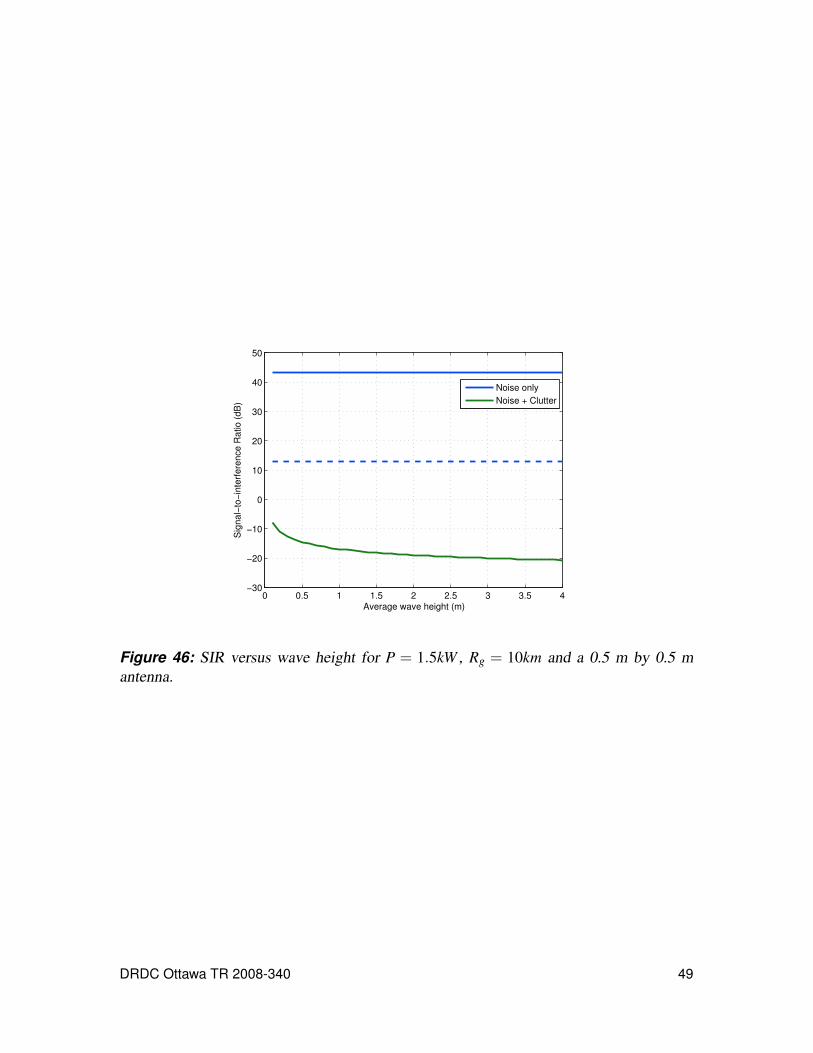
0 0.5 1 1.5 2 2.5 3 3.5 4−30
−20
−10
0
10
20
30
40
50
Average wave height (m)
Sig
nal−
to−
inte
rfere
nce R
atio (
dB
)
Noise only
Noise + Clutter
Figure 46: SIR versus wave height for P = 1.5kW , Rg = 10km and a 0.5 m by 0.5 m
antenna.
DRDC Ottawa TR 2008-340 49

9 Simulation of UAV Detection of Small
Boats
A monostatic UAV radar for small boat detection was simulated in RLSTAP. The goal of
this simulation was to generate datacubes to evaluate the performance of STAP processing.
The modelled antenna was a 0.4 m-by-0.4 m side-looking, rectangular array with 3 sub-
apertures on receive and 0.1 m spacing between sub-apertures. The transmitted waveform
had a PRF of 4 kW with a pulse width of 40 µs. Coherent pulse intervals of 32 pulses were
transmitted, and the peak transmitted power was 1.5 kW. The UAV is assumed to be flying
above the ship. Simulations were run for a small boat RCS of 1 m2, which is the median
value for monostatic small boat RCS from Figure A.5. The boat is travelling towards
the ship. The littoral clutter background consisted of both land clutter and sea clutter in
sea state 3. Two different target ranges were considered, 5 km and 10 km. In addition,
two different values for the radar azimuth angle were considered, 0˚ and 45˚. Thus four
different simulation scenarios were generated, as specified in Table 8. The range-Doppler
map for Scenario 1 is shown in Figure 47.
Table 8: Simulation scenarios for UAV radar detection of small boats.
Scenario Target Range (km) Azimuth angle (˚)
1 5 0
2 10 0
3 5 45
4 10 45
Figures 48-51 show the improvement factors for the four scenarios considered. Table 9
presents the minimum detectable velocity for each of the four scenarios. As shown in Fig-
ure 48, under Scenario 1 Factored STAP has higher IF values at lower frequencies than
Adapt-then-filter. Both STAP techniques have IFs that are approximately 10 dB greater
than that of Doppler processing, except in the clutter notch. In Scenario 2, the IF of Fac-
tored STAP is slightly higher than that of Adapt-then-filter at lower Doppler frequencies,
as shown in Figure 49. In this case, the performance of the STAP methods is 20 dB better
than that of Doppler processing. Figure 50 shows the IFs for Scenario 3. Once again, Fac-
tored STAP has better performance than Adapt-then-filter. Finally, in Scenario 4, as shown
in Figure 51, the IFs are seen to be similar to those from Scenarios 2 and 3.
Table 9 shows minimum detectable velocity and usable Doppler space fraction for all four
scenarios. In all scenarios, Doppler processing has the largest MDV and smallest UDSF,
while Factored STAP has the smallest MDV and largest UDSF. The use of STAP provides
a significant improvement in MDV. In Scenario 1, the improvement is 0.9 m/s, and in
Scenario 4, the improvement is 2.8 m/s.
50 DRDC Ottawa TR 2008-340

Table 9: Minimum detectable velocity (MDV) and usable Doppler space fraction (UDSF)
for small boat detection scenarios.
Scenario 1 Scenario 2 Scenario 3 Scenario 4
Doppler MDV (m/s) 4.7 5.6 5.6 6.6
processing UDSF (%) 84.4 81.3 81.3 78.1
Adapt-then-filter MDV (m/s) 3.8 3.8 4.7 4.7
UDSF (%) 87.5 87.5 84.4 84.4
Factored MDV (m/s) 2.8 2.8 2.8 3.8
STAP UDSF (%) 90.6 90.6 90.6 87.5
Doppler (Hz)
Ra
ng
e (
km
)
−1000 −500 0 500 10002.5
5
7.5
10
12.5
15
17.5
20
−14
−12
−10
−8
−6
−4
Target
Figure 47: Range-Doppler map of returns from Scenario 1.
DRDC Ottawa TR 2008-340 51
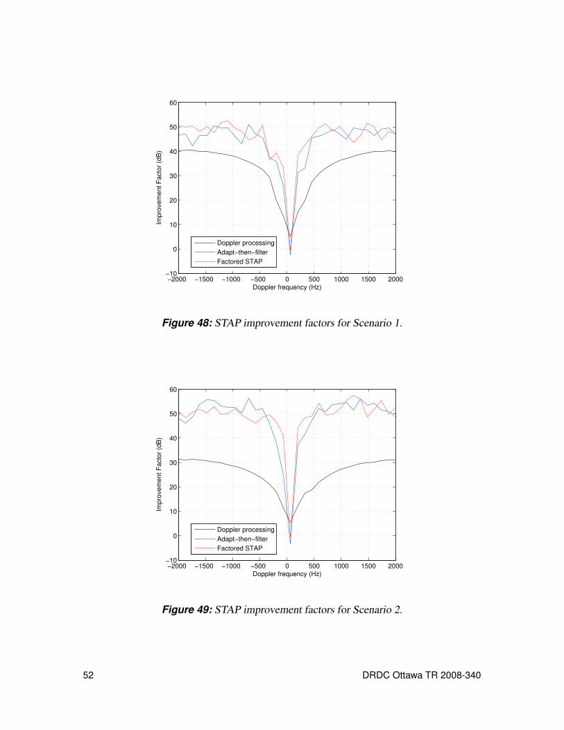
−2000 −1500 −1000 −500 0 500 1000 1500 2000−10
0
10
20
30
40
50
60
Doppler frequency (Hz)
Impro
vem
ent F
acto
r (d
B)
Doppler processing
Adapt−then−filter
Factored STAP
Figure 48: STAP improvement factors for Scenario 1.
−2000 −1500 −1000 −500 0 500 1000 1500 2000−10
0
10
20
30
40
50
60
Doppler frequency (Hz)
Impro
vem
ent F
acto
r (d
B)
Doppler processing
Adapt−then−filter
Factored STAP
Figure 49: STAP improvement factors for Scenario 2.
52 DRDC Ottawa TR 2008-340

−2000 −1500 −1000 −500 0 500 1000 1500 20000
10
20
30
40
50
60
Doppler frequency (Hz)
Impro
vem
ent F
acto
r (d
B)
Doppler processing
Adapt−then−filter
Factored STAP
Figure 50: STAP improvement factors for Scenario 3.
−2000 −1500 −1000 −500 0 500 1000 1500 20000
10
20
30
40
50
60
70
Doppler frequency (Hz)
Impro
vem
ent F
acto
r (d
B)
Doppler processing
Adapt−then−filter
Factored STAP
Figure 51: STAP improvement factors for Scenario 4.
DRDC Ottawa TR 2008-340 53
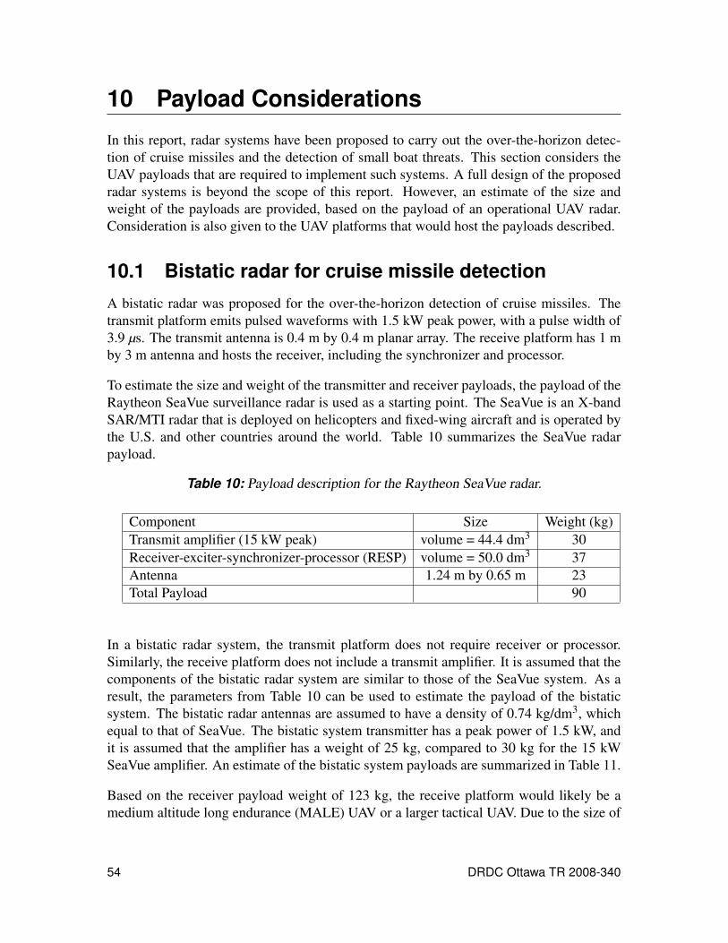
10 Payload Considerations
In this report, radar systems have been proposed to carry out the over-the-horizon detec-
tion of cruise missiles and the detection of small boat threats. This section considers the
UAV payloads that are required to implement such systems. A full design of the proposed
radar systems is beyond the scope of this report. However, an estimate of the size and
weight of the payloads are provided, based on the payload of an operational UAV radar.
Consideration is also given to the UAV platforms that would host the payloads described.
10.1 Bistatic radar for cruise missile detection
A bistatic radar was proposed for the over-the-horizon detection of cruise missiles. The
transmit platform emits pulsed waveforms with 1.5 kW peak power, with a pulse width of
3.9 µs. The transmit antenna is 0.4 m by 0.4 m planar array. The receive platform has 1 m
by 3 m antenna and hosts the receiver, including the synchronizer and processor.
To estimate the size and weight of the transmitter and receiver payloads, the payload of the
Raytheon SeaVue surveillance radar is used as a starting point. The SeaVue is an X-band
SAR/MTI radar that is deployed on helicopters and fixed-wing aircraft and is operated by
the U.S. and other countries around the world. Table 10 summarizes the SeaVue radar
payload.
Table 10: Payload description for the Raytheon SeaVue radar.
Component Size Weight (kg)
Transmit amplifier (15 kW peak) volume = 44.4 dm3 30
Receiver-exciter-synchronizer-processor (RESP) volume = 50.0 dm3 37
Antenna 1.24 m by 0.65 m 23
Total Payload 90
In a bistatic radar system, the transmit platform does not require receiver or processor.
Similarly, the receive platform does not include a transmit amplifier. It is assumed that the
components of the bistatic radar system are similar to those of the SeaVue system. As a
result, the parameters from Table 10 can be used to estimate the payload of the bistatic
system. The bistatic radar antennas are assumed to have a density of 0.74 kg/dm3, which
equal to that of SeaVue. The bistatic system transmitter has a peak power of 1.5 kW, and
it is assumed that the amplifier has a weight of 25 kg, compared to 30 kg for the 15 kW
SeaVue amplifier. An estimate of the bistatic system payloads are summarized in Table 11.
Based on the receiver payload weight of 123 kg, the receive platform would likely be a
medium altitude long endurance (MALE) UAV or a larger tactical UAV. Due to the size of
54 DRDC Ottawa TR 2008-340

Table 11: Payload estimate for the bistatic radar for cruise missile detection.
Platform Component Size Weight (kg)
Transmitter Transmit amplifier (1.5 kW peak) volume = 44.4 dm3 25
Exciter-synchronizer volume = 50.0 dm3 12
Antenna 0.4 m by 0.4 m 5
Total Payload 42
Receiver RESP volume = 50.0 dm3 37
Antenna 1 m by 3 m 86
Total Payload 123
the receive antenna, a MALE UAV platform would be required to host the antenna. The
weight of the UAV platform would need to be large enough so that a side-mounted antenna
does not destabalize the platform in-flight. Furthermore, the 3 m length of the antenna
necessitates the use of a longer airframe.
The transmit platform would likely be a tactical UAV. The payload weight and the relatively
modest size of the antenna allow flexibility is choosing a platform. The UAV control ground
stations for both platforms would need to be located on the ship. This would allow for UAV
radar detections at the receiver to be used to cue the shipborne radar. The ship-based ground
station for the transmitter would also be used to deploy the transmitter in the direction of
the expected threat.
Current UAV radars are monostatic, and as a result, the design of the UAV radar system
would need to take bistatic operation into account. In particular, timing and synchroniza-
tion between the transmitter and receiver would need to be carefully considered, in order
to benefit from the advantages of coherent signal processing.
10.2 Monostatic radar for small boat detection
For small boat detection, a monostatic radar was proposed with a peak power of 1.5 kW
and a pulse width of 50 µs. The antenna is a 0.4 m by 0.4 m planar array. Once again, the
Raytheon SeaVue radar is used as a starting point for estimating the radar payload. The
estimates are presented in Table 12. The estimated payload weight of 67 kg and the modest
antenna size suggest that the radar platform would likely be a tactical UAV.
DRDC Ottawa TR 2008-340 55
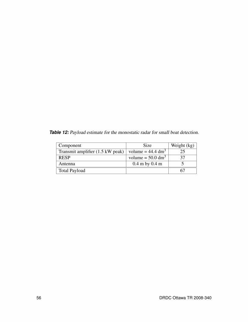
Table 12: Payload estimate for the monostatic radar for small boat detection.
Component Size Weight (kg)
Transmit amplifier (1.5 kW peak) volume = 44.4 dm3 25
RESP volume = 50.0 dm3 37
Antenna 0.4 m by 0.4 m 5
Total Payload 67
56 DRDC Ottawa TR 2008-340

11 Conclusions
This report evaluated the detection performance of UAV radar systems for two distinct
applications, the over-horizon detection of cruise missiles and the detection of small boat
threats. In both cases, the goal was to develop a UAV radar that would meet the required
detection performance while reducing the size and power of the UAV payload.
For the cruise missile detection problem, a cruise missile with an RCS of 0.1 m2 and a
velocity of Mach 0.75 was assumed. The goal of the radar system was to detect the threat
when it passed through a rectangular barrier. Against this threat, a previous analysis had
proposed a bistatic radar with a receiver located above the ship and the transmitter deployed
in the direction of the expected threat. In this study, the performance of this bistatic system
was analyzed using simulation in RLSTAP. The use of high-PRF waveform allowed for the
unambiguous Doppler estimate of a cruise missile travelling at speeds up to Mach 2. A
ship self-defence configuration and two area air defence configurations were considered.
For ship self defence, the simulation analysis showed that MDV was 46.3 m/s when STAP
processing was employed. Furthermore, it was shown that the radar failed to detect crossing
targets, which are less of a threat in ship self-defence. For area air defence, the MDV was
also 46.3 m/s with STAP processing. However, targets heading for the ship-of-interest at an
angle may not be detected by the UAV radar, due to the larger bistatic angles associated with
the radar geometry. Therefore, the UAV radar is effective in providing ship self defence
capability, but may be impeded in providing area air defence if the bistatic geometries are
not favourable. It is estimated that transmitter payload has a weight of 42 kg and would
require a tactical UAV as a platform. The receiver payload has a weight of 123 kg and
would require a MALE UAV platform.
For small boat detection, the monostatic and bistatic RCS of the Legend small boat was
analyzed using the software Rapport. It was shown that the median monostatic RCS was
1 m2. A parametric analysis of a monostatic UAV radar was carried out. The resulting radar
was modelled in RLSTAP, using a low PRF waveform. It was seen that Factored STAP
had better performance against the small boat threat, both in terms of higher improvement
factor and lower MDV. For four simulated scenarios, Factored STAP resulted in MDVs
between 2.8 m/s and 3.8 m/s. STAP provides significant benefit in the detection of small
boats by decreasing the MDV. Further work in this area would involve verifying UAV radar
performance using experimental data. For small boat detection, the radar payload has an
estimated weight of 67 kg and would require a tactical UAV as a platform.
DRDC Ottawa TR 2008-340 57

This page intentionally left blank.
58 DRDC Ottawa TR 2008-340

Annex A: Bistatic Small Boat RCS
This annex presents an analysis of the bistatic RCS of the Legend small boat. This analysis
could be used in the future to aid in the design of bistatic UAV radar systems for small boat
detection.
Figures A.1 to A.4 show Mercator plots of the bistatic RCS of the Legend boat for various
transmitter positions. In all cases, φi=0˚. As was the case for the monostatic RCS, the
bistatic RCS varies greatly with elevation angle. In Figure A.1, θi=10˚, and the bistatic
RCS has a limited number of regions with large values. The most prominent occurs when
the receiver is located near θr = 10˚ and φr = 180˚. In Figure A.2, θi = 30˚. In this case,
there is a larger region where the RCS is large, although the RCS may vary significantly for
small changes in transmitter location. When θi = 60˚, as shown in Figure A.3, the bistatic
RCS is greater than 25 dB for almost all receiver locations between θr = 40˚ and 80˚. In
Figure A.4, θi = 90˚, and the bistatic RCS is largest for receiver locations between θr = 50˚
and 80˚, although the RCS values are smaller than those in Figure A.3.
φr (degrees)
θr (
degre
es)
0 50 100 150 200 250 300 350
0
10
20
30
40
50
60
70
80
90
RC
S (
dB
sm
)
−10
−5
0
5
10
15
20
25
30
Figure A.1: Bistatic RCS in dBsm when the transmitter location is specified by θi=10˚ and
φi=0˚.
Another approach to analyzing the bistatic RCS data is to consider the RCS as a function
of bistatic angle. For all RCS measurements, the bistatic angle is computed for each
combination of the transmitter and receiver positions. For each bistatic angle, the median
and various percentiles of bistatic RCS can then be computed. This approach reduces the
number of variables in the analysis. It also shows if there are particular bistatic angles that
DRDC Ottawa TR 2008-340 59

φr (degrees)
θr (
degre
es)
0 50 100 150 200 250 300 350
0
10
20
30
40
50
60
70
80
90
RC
S (
dB
sm
)
−10
−5
0
5
10
15
20
25
30
Figure A.2: Bistatic RCS in dBsm when the transmitter location is specified by θi=30˚ and
φi=0˚.
φr (degrees)
θr (
degre
es)
0 50 100 150 200 250 300 350
0
10
20
30
40
50
60
70
80
90
RC
S (
dB
sm
)
−10
−5
0
5
10
15
20
25
30
Figure A.3: Bistatic RCS in dBsm when the transmitter location is specified by θi=60˚ and
φi=0˚.
60 DRDC Ottawa TR 2008-340
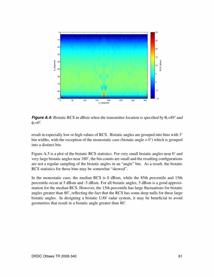
φr (degrees)
θr (
degre
es)
0 50 100 150 200 250 300 350
0
10
20
30
40
50
60
70
80
90
RC
S (
dB
sm
)
−10
−5
0
5
10
15
20
25
30
Figure A.4: Bistatic RCS in dBsm when the transmitter location is specified by θi=89˚ and
φi=0˚.
result in especially low or high values of RCS. Bistatic angles are grouped into bins with 3˚
bin widths, with the exception of the monostatic case (bistatic angle = 0˚) which is grouped
into a distinct bin.
Figure A.5 is a plot of the bistatic RCS statistics. For very small bistatic angles near 0˚ and
very large bistatic angles near 180˚, the bin counts are small and the resulting configurations
are not a regular sampling of the bistatic angles in an “angle” bin. As a result, the bistatic
RCS statistics for these bins may be somewhat “skewed”.
In the monostatic case, the median RCS is 0 dBsm, while the 85th percentile and 15th
percentile occur at 5 dBsm and -5 dBsm. For all bistatic angles, 5 dBsm is a good approxi-
mation for the median RCS. However, the 15th percentile has large fluctuations for bistatic
angles greater than 80˚, reflecting the fact that the RCS has some deep nulls for these large
bistatic angles. In designing a bistatic UAV radar system, it may be beneficial to avoid
geometries that result in a bistatic angle greater than 80˚.
DRDC Ottawa TR 2008-340 61

0 20 40 60 80 100 120 140 160 180−50
−40
−30
−20
−10
0
10
20
30
40
50
bistatic angle (degrees)
RC
S (
dB
sm
)
85th percentile
median
15th percentile
Figure A.5: RCS statistics for 10 GHz, VV polarization. Monostatic RCS values are
indicated by asterisks.
62 DRDC Ottawa TR 2008-340

References
[1] Thomson, A. and Riseborough, E. (2006), Equipment and Measurements for
Evaluating RF Performance Prediction at the SISWS Environment Modelling Trials,
(DRDC Ottawa TM 2006-149) Defence R&D Canada – Ottawa.
[2] Tsunoda, S., Pace, F., Stence, J., Woodring, M., Hensley, W., Doerry, A., and
Walker, B. (2000), Lynx: A High-Resolution Synthetic Aperture Radar, In
Proceedings of the 2000 IEEE Aerospace Conference, pp. 51–58.
[3] Giret, R., Jeuland, H., and Enert, P. (2004), A Study of a 3D-SAR concept for a
millimeter wave imaging radar onboard an UAV, In Proceedings of First European
Radar Conference, pp. 201–204.
[4] Goktogan, A.H., Booker, G., and Sukkarieh, S. (2006), Field and Service Robotics,
pp. 311–320, Springer Berlin.
[5] Scott, R. (2003), Russia’s anti-ship arsenal targets export markets, Jane’s Navy
International.
[6] Scott, R. (2005), Anti-ship weapons updated to target the shore, Jane’s Navy
International.
[7] Lok, J. Janssen (2005), Modern navy missiles march on, International Defence
Review.
[8] Moo, P.W. (2001), Bistatic RCS Predictions for a Cruise Missile, (DREO TM
2001-167) Defence R&D Canada – Ottawa.
[9] Moo, P.W. (2006), UAV Radar Concepts for Over-the-Horizon Detection of
Low-Altitude Threats, (DRDC Ottawa TM 2006-254) Defence R&D Canada –
Ottawa.
[10] Walker, D. (2000), Experimentally motivated model for low-grazing angle radar
Doppler spectra of the sea surface, IEE Proceedings on Radar, Sonar and
Navigation, 147(3), 114–120.
[11] Walker, D. (2001), Doppler modelling of radar sea clutter, IEE Proceedings on
Radar, Sonar and Navigation, 148(2), 73–80.
[12] Willis, N.J. (1995), Bistatic Radar, Technology Services Corp.
[13] Moo, P.W. (2001), Properties of Bistatic Clutter Ridges with Applications to
Space-Based Radar, (DREO TM 2001-139) Defence R&D Canada – Ottawa.
[14] Hughes, S. (2001), Procedure for creating land cover data for use with RLSTAP,
(DREO TN 2001-207) Defence R&D Canada – Ottawa.
DRDC Ottawa TR 2008-340 63

[15] Horst, M., Dyer, F., and Tuley, M. (1978), Radar Sea Clutter Model, In IEE
International Conference on Antennas and Propagation, pp. 6–10.
[16] Brennan, L. and Reed, I. (1973), Theory of adaptive radar, IEEE Trans. On
Aerospace and Elec. Systems, 9, 237–251.
[17] Ward, J. (1994), Space-time adaptive processing for airborne radar, (Technical
Report 1015) MIT Lincoln Laboratory.
[18] Eaves, J.L. and Ready, E.K. (1987), Principals of Modern Radar, New York:
Chapman and Hall.
[19] Ward, K., Baker, C., and Watts, S. (1990), Maritime Surveillance Radar; Part 1:
Radar scattering from the ocean surface, Proceedings of the IEE, 137 (F), 51–62.
64 DRDC Ottawa TR 2008-340
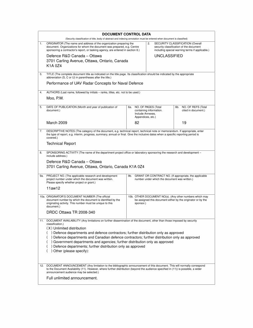
DOCUMENT CONTROL DATA(Security classification of title, body of abstract and indexing annotation must be entered when document is classified)
1. ORIGINATOR (The name and address of the organization preparing the
document. Organizations for whom the document was prepared, e.g. Centre
sponsoring a contractor’s report, or tasking agency, are entered in section 8.)
Defence R&D Canada – Ottawa
3701 Carling Avenue, Ottawa, Ontario, Canada
K1A 0Z4
2. SECURITY CLASSIFICATION (Overall
security classification of the document
including special warning terms if applicable.)
UNCLASSIFIED
3. TITLE (The complete document title as indicated on the title page. Its classification should be indicated by the appropriate
abbreviation (S, C or U) in parentheses after the title.)
Performance of UAV Radar Concepts for Naval Defence
4. AUTHORS (Last name, followed by initials – ranks, titles, etc. not to be used.)
Moo, P.W.
5. DATE OF PUBLICATION (Month and year of publication of
document.)
March 2009
6a. NO. OF PAGES (Total
containing information.
Include Annexes,
Appendices, etc.)
82
6b. NO. OF REFS (Total
cited in document.)
19
7. DESCRIPTIVE NOTES (The category of the document, e.g. technical report, technical note or memorandum. If appropriate, enter
the type of report, e.g. interim, progress, summary, annual or final. Give the inclusive dates when a specific reporting period is
covered.)
Technical Report
8. SPONSORING ACTIVITY (The name of the department project office or laboratory sponsoring the research and development –
include address.)
Defence R&D Canada – Ottawa
3701 Carling Avenue, Ottawa, Ontario, Canada K1A 0Z4
9a. PROJECT NO. (The applicable research and development
project number under which the document was written.
Please specify whether project or grant.)
11aw12
9b. GRANT OR CONTRACT NO. (If appropriate, the applicable
number under which the document was written.)
10a. ORIGINATOR’S DOCUMENT NUMBER (The official
document number by which the document is identified by the
originating activity. This number must be unique to this
document.)
DRDC Ottawa TR 2008-340
10b. OTHER DOCUMENT NO(s). (Any other numbers which may
be assigned this document either by the originator or by the
sponsor.)
11. DOCUMENT AVAILABILITY (Any limitations on further dissemination of the document, other than those imposed by security
classification.)
( X ) Unlimited distribution
( ) Defence departments and defence contractors; further distribution only as approved
( ) Defence departments and Canadian defence contractors; further distribution only as approved
( ) Government departments and agencies; further distribution only as approved
( ) Defence departments; further distribution only as approved
( ) Other (please specify):
12. DOCUMENT ANNOUNCEMENT (Any limitation to the bibliographic announcement of this document. This will normally correspond
to the Document Availability (11). However, where further distribution (beyond the audience specified in (11)) is possible, a wider
announcement audience may be selected.)
Full unlimited announcement.

13. ABSTRACT (A brief and factual summary of the document. It may also appear elsewhere in the body of the document itself. It is highly
desirable that the abstract of classified documents be unclassified. Each paragraph of the abstract shall begin with an indication of the
security classification of the information in the paragraph (unless the document itself is unclassified) represented as (S), (C), (R), or (U).
It is not necessary to include here abstracts in both official languages unless the text is bilingual.)
This report analyzes the performance of a bistatic uninhabited aerial vehicle (UAV) radar to detect
cruise missile threats beyond a ship’s horizon. The bistatic system, together with adaptive signal
processing is shown to provide self-defence capabilities against targets that are heading towards
the ship. For area air defence, the UAV radar may not be able to detect some targets, depending
on the bistatic geometry. A monostatic UAV radar for small boat defence is also developed. The
radar cross section (RCS) of a small boat is modelled, and it is shown that the median monostatic
RCS is 1 m2. Performance of the UAV radar is analyzed by simulating the small boat scenario
in RLSTAP. With the use of Factored space-time adaptive processing (STAP) to reduce clutter
power, the resulting minimum detectable velocity is shown to be between 2.8 m/s and 3.8 m/s.
Payload sizes and weights are estimated for the proposed radars.
14. KEYWORDS, DESCRIPTORS or IDENTIFIERS (Technically meaningful terms or short phrases that characterize a document and could
be helpful in cataloguing the document. They should be selected so that no security classification is required. Identifiers, such as
equipment model designation, trade name, military project code name, geographic location may also be included. If possible keywords
should be selected from a published thesaurus. e.g. Thesaurus of Engineering and Scientific Terms (TEST) and that thesaurus identified.
If it is not possible to select indexing terms which are Unclassified, the classification of each should be indicated as with the title.)
Uninhabited aerial vehicles (UAVs)
bistatic radar
cruise missile detection
small boat detection


![IntegratedSimulationEnvironmentforUnmannedAutonomous ...SimulationEnvironment (MUSE) [17], the Naval Air Systems Command (NAVAIR) UAV Unmanned Combat Aerial Vehi-cle (UCAV) Distributed](https://img.pdfslide.net/doc/110x75/60d9a0df17e0d57eda1fcb5b/integratedsimulationenvironmentforunmannedautonomous-simulationenvironment-muse.jpg)