Embed Size (px)
Citation preview

Department of Computer Science
Gonzalo Iglesias Aguiño
Performance of VoIP strategies for hybrid Mobile Ad Hoc Networks
Computer Networks D-level thesis (20p)
Date: 061221
Supervisor: Andreas Kassler
Examiner: Kerstin Andersson
Serial Number: D2007:05
Karlstads universitet 651 88 Karlstad Tfn 054-700 10 00 Fax 054-700 14 60
[email protected] www.kau.se
Computer Science
Master’s Project
2007:05
Gonzalo Iglesias Aguiño
Performance of VoIP strategies for hybrid
Mobile Ad Hoc Networks

3
Performance of VoIP strategies for hybrid
Mobile Ad Hoc Networks
Gonzalo Iglesias Aguiño
© 2007, Gonzalo Iglesias Aguiño and Karlstad University
iv
This report is submitted in partial fulfillment of the requirements for the
Bachelor’s degree in Computer Science. All material in this report which is
not my own work has been identified and no material is included for which
a degree has previously been conferred.
Gonzalo Iglesias Aguiño
Approved,
Advisor: Andreas J. Kassler
Examiner: Kerstin Andersson
5
Abstract
Last decade, a lot of research has been done in wireless communication technologies. Mobile
nodes such personal digital assistants (PDAs), notebooks and cell phones are nowadays used
in human’s daily life.
MANETs are networks consisting of two or more mobile nodes equipped with wireless
communication and networking capabilities, but they don’t have any network centrilized
infrastructure.
In last few years, MANETs have been emerged to be an important researched subject in the
field of wireless networking.
MANETs are autonomous; however they can communicate with other external networks such
the internet. They are linked to such external networks by mobile nodes acting as gateways.
This kind of networks is known as hybrid MANETs.
Voice over Internet Protocol (VoIP), is a technology that allows you to make voice calls using
a Internet connection instead of a regular (or analog) phone line.
The goal of this thesis is evaluate the performance of VoIP strategies for hybrid MANETs.
Two different aspects are evaluated, the session establishment performance and the voice
quality.
Network Simulator 2 is used to run several simulations, two different applications are used to
run voice simulations (Session Initiation Protocol and Exponential traffic generator). We
evaluate two different cases for voice traffics, voice calls between two MANET nodes and
voice calls between MANET nodes and external nodes.
After running the simulations, there are some performance parameters which will reveal the
results. The key findings of the simulations are: adding gateways, number of voice traffic
flows and the number of hops between source and destinations. There are some interesting
results which reveal for example, that adding gateways is not always beneficial.

6
Contents
1 Introduction ..................................................................................................................... 13
1.1 SIP services in internet connected MANETS.......................................................... 13
1.2 Key findings (results) of the simulations................................................................. 15
1.3 Document overview................................................................................................. 16
2 Background...................................................................................................................... 17
2.1 Gateway discovery................................................................................................... 17 2.1.1 Proactive Approach................................................................................................................ 18 2.1.2 Reactive Approach................................................................................................................. 18 2.1.3 Hybrid Approach.................................................................................................................... 19
2.2 Routing protocols..................................................................................................... 20 2.2.1 Proactive Routing Protocols................................................................................................... 21 2.2.2 Reactive Routing Protocols.................................................................................................... 22 2.2.3 Hybrid Routing Protocols ...................................................................................................... 22 2.2.4 Comparison of the routing protocols in MANETS ................................................................ 22
2.3 AODV-UU............................................................................................................... 23 2.3.1 Introduction to AODV-UU .................................................................................................... 23 2.3.2 AODV Operation ................................................................................................................... 23
2.4 SIP (session initiation protocol)............................................................................... 26 2.4.1 Introduction............................................................................................................................ 26 2.4.2 SIP components...................................................................................................................... 27 2.4.3 How SIP works ...................................................................................................................... 29 2.4.4 SIP methods ........................................................................................................................... 29 2.4.5 SIP message codes ................................................................................................................. 31
3 Network Simulator 2....................................................................................................... 35
3.1 Introduction.............................................................................................................. 35
3.2 Running simulations ................................................................................................ 37
3.3 Node structure.......................................................................................................... 40 3.3.1 Wired nodes ........................................................................................................................... 40 3.3.2 Wireless nodes ....................................................................................................................... 41
3.4 Links ........................................................................................................................ 42
3.5 Packets ..................................................................................................................... 43
3.6 Agents ...................................................................................................................... 45
3.7 Radio Propagation Models ...................................................................................... 46
3.8 Communication range calculation ........................................................................... 47

7
3.9 Wired cum wireless simulation ............................................................................... 48
3.10 Trace file structure................................................................................................... 48
4 Design and Implementation ........................................................................................... 52
4.1 Introduction and goals ............................................................................................. 52
4.2 Areas of concern ...................................................................................................... 53 4.2.1 Tcl Scripts: ............................................................................................................................. 53 4.2.2 Perl Scripts: ............................................................................................................................ 53 4.2.3 Plotted graphs:........................................................................................................................ 53 4.2.4 Main contributions ................................................................................................................. 53
4.3 Implementation and configuration of VoIP in Hybrid MANETs in NS2 ............... 55 4.3.1 Network topology .................................................................................................................. 55 4.3.2 Traffic and agents................................................................................................................... 64 4.3.3 Events schedule...................................................................................................................... 69
4.4 Post-tracing .............................................................................................................. 71 4.4.1 Exponential packet delay ....................................................................................................... 72 4.4.2 SIP calls set up delay ............................................................................................................. 72 4.4.3 SIP hops number .................................................................................................................... 73 4.4.4 Dropped packet and reasons................................................................................................... 74
4.5 Performance Parameters and scalability .................................................................. 75 4.5.1 Background traffic ................................................................................................................. 76 4.5.2 SIP invitation calls ................................................................................................................. 77 4.5.3 Scalability of VoIP call setup and delay limits proposed....................................................... 80
5 Evaluation of simulations ............................................................................................... 82
5.1 Simulation Scenarios ............................................................................................... 82
5.2 Traffic Scenario ....................................................................................................... 84 5.2.1 Background Traffic Scenario ................................................................................................. 84 5.2.2 SIP calls traffic scenario......................................................................................................... 85
5.3 Simulation Evaluation ............................................................................................. 87 5.3.1 Evaluation of Session Call Establishment.............................................................................. 87 5.3.2 Evaluation of Voice Quality................................................................................................. 100
6 Conclusions and future work ....................................................................................... 112
6.1 Conclusions............................................................................................................ 112
6.2 Future work............................................................................................................ 114
References ............................................................................................................................. 116
7 Appendix ........................................................................................................................ 118
A Common Abbreviations................................................................................................ 118
B Simulation Scripts code ................................................................................................ 118
B.1 Main Simulation script .......................................................................................... 118 B.1.1 Base station definition code ................................................................................................. 128 B.1.2 Nodes placement .................................................................................................................. 132 B.1.3 SIP nodes ............................................................................................................................. 133 B.1.4 Exponential nodes ................................................................................................................ 137
8
C Post-tracing details........................................................................................................ 145
C.1 Post-tracing code files............................................................................................ 145 C.1.1 Perl script to extract the exponential data and each SIP setup delay from each simulation . 145 C.1.2 Perl script to make the average of Exponential and SIP values already extracted with Perl
script C.1.1. .......................................................................................................................... 150 C.1.3 Perl script to count the number of SIP hops......................................................................... 155 C.1.4 Perl script to extract the exponential information of each exponential traffic flow ............. 157 C.1.5 Perl script to calculate the percentage of valid calls............................................................. 163 C.1.6 Perl script to create SIP user nodes randomly...................................................................... 164 C.1.7 Perl script to extract the exponential packet loss rate classified in intra and outgoing traffic
flows..................................................................................................................................... 165
C.2 Post-tracing data .................................................................................................... 166
D Graphs............................................................................................................................ 172
D.1 About voice traffic flows ....................................................................................... 172 D.1.1 End to end delay................................................................................................................... 172 D.1.2 Packet loss rate..................................................................................................................... 177 D.1.3 Dropped packets and reasons ............................................................................................... 180
D.2 About SIP............................................................................................................... 182 D.2.1 SIP call setup........................................................................................................................ 182 D.2.2 Calls accepted each 100 milliseconds .................................................................................. 183 D.2.3 Call block probability........................................................................................................... 186 D.2.4 Call block probability within 2 seconds............................................................................... 187 D.2.5 Call block probability within 10 seconds............................................................................. 188 D.2.6 SIP invitation attempts ......................................................................................................... 189 D.2.7 SIP invitation attempts and reasons ..................................................................................... 190 D.2.8 SIP number of hops.............................................................................................................. 195
9
List of Figures
Figure 1: SIP performance ,two SIP users in same domain.............................................. 29
Figure 2 : Internal’s view of theNetwork Simulator 2 [22] .............................................. 37
Figure 3: User’s view of an network simulation [23]....................................................... 37
Figure 4: Wired node structure in NS2 ............................................................................. 40
Figure 5:Wireless node structure in NS2 .......................................................................... 41
Figure 6: Link in NS-2 ...................................................................................................... 42
Figure 7: Packet structure in NS-2 .................................................................................... 44
Figure 8: SIP invitation event tasks .................................................................................. 70
Figure 9:Basic Scenario .................................................................................................... 83
Figure 10: Scenarios with 1 (a), 2 (b) and 4 (c) gateways ................................................ 83
Figure 11: SIP time schedule ............................................................................................ 86
Figure 12: Call Setup Delay 2hops ................................................................................... 88
Figure 13: Call Setup Delay 7hops ................................................................................... 89
Figure 14: Call Setup Delay 1 gateway............................................................................ 90
Figure 15:Accepted calls until time for 2 hops,4 flows simulation ................................. 91
Figure 16: Accepted calls until time for 5 hops and 24 flows simulation........................ 92
Figure 17:Call block probability 7hops simulations ......................................................... 94
Figure 18:Call block probability within 2 seconds in 7 hops simulations ........................ 94
Figure 19:Call block probabilities 2(a) and 10(b) seconds 4 hops simulations ................ 95
Figure 20: Invitation attempts in 2(a) and 7(b) hops simulations ..................................... 96
Figure 21: Invitation Attempts for 2 hops with one (a), two(b) and three(c) gateways.... 97
Figure 22:Invitation attempts for 7 hops with one (a), two (b) and three (c) gateways... 97
Figure 23: Number of SIP hops for 2 hops of background flows simulations.................. 99
Figure 24: Number of SIP hops for 7 hops of background flows simulations.................. 99
Figure 25: Packet loss rate for 2(a) and 5(b) hops simulations....................................... 101
Figure 26: Packet loss rate for intra flows for 2 hops(a) and 5 hops(b).......................... 102
Figure 27: Outgoing traffic nodes for two hops simulations .......................................... 103
Figure 28: Outgoing traffic nodes for six hops simulations............................................104
Figure 29:Packet loss rate for outgoing flows for 2(a) and 5(b) hops ............................ 105
Figure 30:Packet loss rate for intra and outgoing flows for 1(a) and 4(b) gateways and
5hops simulations....................................................................................... 105
10
Figure 31: Packets dropped and reasons for 1(a),2(b) and 4(c) gateways and 8
background traffic flows simulations......................................................... 106
Figure 32: Background voice calls delay in 3(a) and 6(a) hops simulations ................. 107
Figure 33:Delay for intra traffic flows for 3(a) and 5(b) hops simulations .................... 108
Figure 34:Delay for outgoing traffic flows for 3(a) and 6(b)hops simulations............... 109
Figure 35:Valid background voice calls in 2 hops simulations ...................................... 110
Figure 36:Valid background voice calls in 4 hops simulations ...................................... 110
Figure 37: Nodes number identifier ................................................................................ 133
Figure 38: Dropped packets and reasons for 8 flows and 1 gateway simulations .......... 180
Figure 39: Dropped packets and reasons for 8 flows and 2 gateways ............................ 181
Figure 40: Dropped packets and reasons for 8 flows and 4 gateways simulations......... 181
Figure 41: SIP invitation attempts and reasons for 3 hops and 1 gateway ..................... 190
Figure 42: SIP invitation attempts and reasons for 3 hops and 2 gateways.................... 190
Figure 43: SIP invitation attempts and reasons for 3 hops and 4 gateways.................... 191
Figure 44: SIP invitation attempts and reasons for 4 hops and 1 gateway ..................... 191
Figure 45: SIP invitation attempts and reasons for 4 hops and 2 gateways simulations 192
Figure 46: SIP invitation attempts and reasons for 4 hops and 4 gateways simulations 193
Figure 47: SIP invitation attempts and reasons for 6 hops and 1 gateway simulation.... 193
Figure 48: SIP invitation attempts and reasons for 6 hops and 2 gateways simulations 194
Figure 49: SIP invitation attempts and reasons for 6 hops and 4 gateways simulations 194
List of Code Lines
11
Code 1: simulator instance ................................................................................................ 38
Code 2: Opening trace files............................................................................................... 38
Code 3: Finish procedure .................................................................................................. 39
Code 4: Starting simulation............................................................................................... 39
Code 5: Link definition in a Tcl script .............................................................................. 42
Code 6: Communication range settings ............................................................................ 47
Code 7: Creating NS object............................................................................................... 55
Code 8: Creating topology and topography ...................................................................... 55
Code 9: Definition and connection of wired nodes........................................................... 57
Code 10: MAC 802.11g definition................................................................................... 59
Code 11: Mobile nodes declaration................................................................................... 60
Code 12: Creating base station.......................................................................................... 63
Code 13: Connecting a base station with a wired network ...............................................64
Code 14: UDP agents definition ....................................................................................... 66
Code 15: Exponential traffic definition............................................................................. 67
Code 16: SIP proxy definition........................................................................................... 68
Code 17: SIP users definition............................................................................................ 68
Code 18: set SIP user to the proxy.................................................................................... 69
Code 19: Schedule for Exponential traffic........................................................................ 69
Code 20: Register SIP users.............................................................................................. 70
Code 21: SIP user sends an invitation............................................................................... 70
Code 22: SIP user sends a bye request.............................................................................. 71
Code 23: Trace file line to get number of hops................................................................. 73
Code 24: Trace file line of dropped packet. ...................................................................... 74

12
List of Tables
Table 1: Agent state information....................................................................................... 45
Table 2: Wired trace format fields .................................................................................... 49
Table 3: Wireless trace format fields. ............................................................................... 51
Table 4: IP wireless trace format fields............................................................................. 51
Table 5: Exponential wireless trace format fields............................................................. 51
Table 6: Code to configure the physical layer .................................................................. 59
Table 7: Default gateway values ....................................................................................... 63
Table 8: G711 and G729 standard specifications ............................................................. 65
Table 9: Examples of trace file lines to extract exponential packets delay ...................... 72
Table 10: Examples of trace file lines to extract SIP call setup delay .............................. 72
Table 11: E-721 ITU Recommendations [29]................................................................... 80
Table 12:Call block probability ........................................................................................ 93
Table 13: Valid background calls for 2 hops simulations...............................................111
Table 14: Valid background calls for 5 hops simulations...............................................112
Table 15: Common Abbreviations .................................................................................. 118
Table 16: End to end delay for intra/outgoing traffic flows............................................ 167
Table 17: Packet loss rate for intra/outgoing traffic flows.............................................. 168
Table 18: Percentage of valid voice flows for intra / outgoing flows............................. 169
Table 19: Call block probability values .......................................................................... 170
Table 20: Call block probability within 2 seconds values ..............................................171
Table 21: Call block probability within 5 seconds values ..............................................171
Table 22: Call block probability within 10 seconds values ............................................ 172

13
1 Introduction
This chapter is the introduction of the thesis and is structured as follows. The section
1.1 is called SIP services in internet connected MANETS and makes an introduction to
Ad Hoc Networks, internet connectivity in Ad Hoc Networks, SIP protocol and the key
problems of this thesis. The section 1.2 is called Key findings and describes the keys to
aim the goals of the dissertation. Section 1.3 is the overview of the report and explains
how the rest of the paper is structured.
1.1 SIP services in internet connected MANETS
A wireless mobile ad hoc network (MANET) is a network consisting of two or more
mobile nodes equipped with wireless communication and networking capabilities, but
they don’t have any network centrilized infrastructure. Each node acts both as a mobile
host and a router, offering to forward traffic on behalf of other nodes within the network.
For this traffic forwarding functionality, a routing protocol for Ad hoc networks is
needed.
Ad hoc networks are self organizing, self healing, distributed networks formed by
autonomous wireless nodes. They can communicate without any centralized control
mechanism. They differ from traditional wireless networks. Tradicional networks need
access points and they have centralized organization, however, Ad Hoc Networks do not
have centralized organization. Nowadays ad hoc networks are very popular subject of
research; however they are originally created for military and emergency purposes.
Ad hoc networks are usually autonomous in connectivity between participating nodes,
but they do not have connectivity to external networks such as the internet. Internet
connectivity is an add-on to standard Ad Hoc Networks.Internet connectivity for
MANETS can be possible, with multi-homed nodes (they can connect to the ad hoc
network and more external networks). These nodes act as gateways between the ad hoc
network and the external network. When there are nodes acting as gateways, it is
necessary to have gateway discovery mechanism. When a MANET is connected to the
internet or another wired network, it is called hybrid MANET.

14
Session initiation protocol (SIP) is an application-layer control protocol that can
establish, modify and terminate multimedia sessions in an IP network. A session could be
a simple two-way telephone call or a multimedia conference session.
The main signaling functions of the SIP protocol are as follows:
Location of an end point: this protocol makes transparent the location of the end users
in multimedia sessions.
Contacting an end point to determine willingness to establish a session.
Exchange of media information to allow session to be established.
Modification of existing media sessions.
Tear-down of existing media sessions.
SIP entities which make session initiation possible are:
SIP end users.
SIP servers which manage all the messages (SIP proxy servers, SIP register servers,
and SIP redirect servers).
The SIP end users have to send a register request to a SIP proxy server, sending the
location information, which means the IP address, the domain, etc…. When a SIP user
wants to invite another SIP user for a session, the SIP caller user send an invitation
request, the SIP proxy checks the information of the SIP called user, when the called user
accept, the session starts directly from the caller to the called. To end the session, one of
the users has to send a bye request.
SIP is not tied to any particular conference control protocol; it is designed to be
independent of the lower-layer transport protocol.
Sip based multimedia applications are even more important for MANETs since mobile
nodes location are changuing every time, and this is one of the most important
characteristics of the MANETs, the transparence of the end points location.
The goal of the dissertation is to analyze the performance of VoIP calls in hybrid
MANETs. When two SIP end users want to communicate in an ad hoc network, they
need to send the SIP control messages through the gateways even if both wireless nodes
belong to that network. This thesis evaluated these situations because of the need to study
the capacity of the internet connected Ad Hoc Network scenario and the need to examine
the performance of SIP call setup and voice call flow quality in order to design a scalable
system.
15
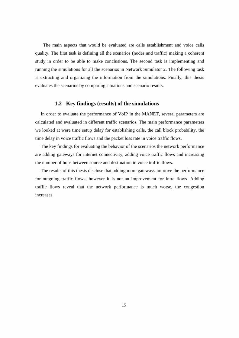
The main aspects that would be evaluated are calls establishment and voice calls
quality. The first task is defining all the scenarios (nodes and traffic) making a coherent
study in order to be able to make conclusions. The second task is implementing and
running the simulations for all the scenarios in Network Simulator 2. The following task
is extracting and organizing the information from the simulations. Finally, this thesis
evaluates the scenarios by comparing situations and scenario results.
1.2 Key findings (results) of the simulations
In order to evaluate the performance of VoIP in the MANET, several parameters are
calculated and evaluated in different traffic scenarios. The main performance parameters
we looked at were time setup delay for establishing calls, the call block probability, the
time delay in voice traffic flows and the packet loss rate in voice traffic flows.
The key findings for evaluating the behavior of the scenarios the network performance
are adding gateways for internet connectivity, adding voice traffic flows and increasing
the number of hops between source and destination in voice traffic flows.
The results of this thesis disclose that adding more gateways improve the performance
for outgoing traffic flows, however it is not an improvement for intra flows. Adding
traffic flows reveal that the network performance is much worse, the congestion
increases.

16
1.3 Document overview
The rest of the document is structured as follows:
Chapter 2 describes gateway discovery and routing protocols. It also describes in
details the routing protocol AODV-UU used in this thesis and the session initiation
protocol (SIP).
Chapter 3 gives an introduction of Network Simulator 2 describing some of its
components and examples of how to use it.
Chapter 4 describes in details the design and implementation of the scripts in Tcl to
run the simulations. This chapter describes the post-tracing process, what the
performance parameters are and how they can be obtained.
Chapter 5 describes all the scenarios and the approaches followed in running the
simulations. The results of the simulations are then evaluated and analyzed using several
graphs.
Finally, chapter 6 gives a brief conclusion of the thesis and suggestions for future
work.
17
2 Background
This chapter is structures as follows. In section 2.1, the different approaches of
gateways discovery are presented (proactive, reactive and hybrid mechanisms). Section
2.2 describe the possible types of routing protocols, having proactive, reactive and
hybrid as routing protocols types. In section 2.3, the routing protocol used in this thesis
(AODV-UU) and its mechanisms of gateway and route discovery and tunneling are
explained. In section 2.4, the session initiation protocol and its entities and functionalities
are presented and explained.
2.1 Gateway discovery
As important as having MANET correctly working is having internet access in a
MANET. To have internet connectivity for MANETs there are some needed things.
Gateways are needed to communicate MANET with exteternal networks. Addressing
autocinfiguration is also needed to detect the gateways, to route to the gateways, to detect
when a node is in the internet or in the MANET. Therefore nodes acting as gateways are
needed. They act as an interface between the MANET and the internet and algorithms to
do it are also needed to manage the situation. By using gateway nodes, the MANETs
network communication is not limited to intra-MANET communication; the network is
also capable of working with other outside networks.
Hence, the term “gateway discovery”, refers to the capability of a MANET to access
the internet or a conventional network and provide global addressing and bidirectional
reach ability to the MANET nodes. [1]
In the last years there have been discussions about what the best approach is to
discover the gateways. Bassically two approaches can be distinguished on who initiates
the discovery: the mobile node or the gateway. Depending on the characteristics of the
network, each approach has advantages and disadvantages. These advantages and
disadvantages will be discussed in the next sections under different kinds of gateway
discovery approaches. [1][3]

18
2.1.1 Proactive Approach
The main principle of this approach is that the gateway starts proactively announces
itself. The gateway therefore periodically broadcast gateway advertisement messages
identifying itself (as gateway). All the nodes in the gateway’s transmission range receive
this broadcast message, and they also relay the message to the other nodes in their
transmission range removing duplicates. Each recipient node also further broadcast this
message to it neighboring nodes. Nodes which already have a route to the gateway, will
update the routing table, and those which do not have a route to the gateway, will create a
new entry in their routing table. This approach involves a very high overhead. One
problem is the well-known “duplicated broadcast messages” problem which also occurs
in routing protocols. However, this problem has can be solved by adding the ID of the
broadcast source node. Due to the redundancy broadcasting, a node may receive the
gateway advertisement message several times. In such a case, where a node receives
more than one gateway advertisement with identical ID, it only considers one. [3]
A disadvantage of this approach is, that the network will have a high overhead of
gateway discovery messages which the nodes will cost power and bandwidth. This
approach can be useful if a very low latency is required to detect a gateway because the
nodes always know which one is the gateway. When there are more than one gateway,
the nodes keep the route to them and they can choose the gateway how they want, usually
they send to the nearest gateway [5]
2.1.2 Reactive Approach
In this approach, gateway discovery is initiated by the mobile node. Most reactive
gateway discovery strategies work with reactive or on-demand MANET routing
protocols.
When a node needs to send a packet outside the MANET, it starts the process of
discovering the gateways. The source node sends a special route request (RREQ_I)
message, by broadcasting it, to the ALL_MANET_GW_MULTICAST address. [3]
If the gateways receive the message, they will answer to the source with a special
route request reply (RREP_I) via unicast.
19
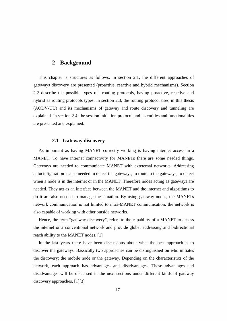
When the source receives the response from the gateways, it then decides based on a
metric which gateway to send the data to, for example depending on the number of hops.
The problem of duplicated packets exits in this approach because of the multicast
forwarding, but it is solved in the same way as in proactive approaches. The route
requests have an ID, so if the nodes receive duplicated packets (with the same id), they
will be discarded.
An advantage of this method is that the network will not have high overhead with the
gateway discovery packets if its nodes do not need a route to a gateway. However, when
they need to acquire a route to a gateway, it takes a longer time to find the route
compared to proactive approaches. Also the neighboring nodes to the gateway will suffer
from overloading because they are involved in the gateway discovery process even if
they do not need the gateway themselves. This happened in proactive approaches as well,
but in reactive approaches the situation is worse, due to the overhead in the neighboting
nodes to the gateway is exactly when we need a good performance.[5]
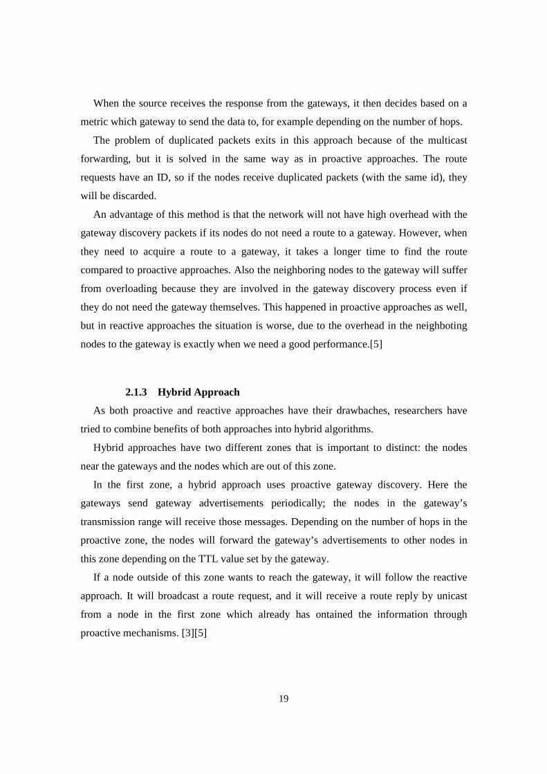
2.1.3 Hybrid Approach
As both proactive and reactive approaches have their drawbaches, researchers have
tried to combine benefits of both approaches into hybrid algorithms.
Hybrid approaches have two different zones that is important to distinct: the nodes
near the gateways and the nodes which are out of this zone.
In the first zone, a hybrid approach uses proactive gateway discovery. Here the
gateways send gateway advertisements periodically; the nodes in the gateway’s
transmission range will receive those messages. Depending on the number of hops in the
proactive zone, the nodes will forward the gateway’s advertisements to other nodes in
this zone depending on the TTL value set by the gateway.
If a node outside of this zone wants to reach the gateway, it will follow the reactive
approach. It will broadcast a route request, and it will receive a route reply by unicast
from a node in the first zone which already has ontained the information through
proactive mechanisms. [3][5]

20
2.2 Routing protocols
Routing protocols refers are needed in order to find a route from a source to a
destination. In this dissertation we deal with specidic decentralized networks such as Ad
Hoc networks, without fixed structure. MANETs have their own routing protocols, some
of them are invented primarily for MANETs, and some were adapted from routing
protocols in used wired networks.
Furthermore, one of the most important goals of these protocols is that they must be
able to work with any topology, because MANETs structure may change at anytime.
The most important differences between MANETS and conventional networks with
respect to routing are:
-Conventional networks are usually static. This is very different from Ad Hoc
networks, where the topology can be very different at different times and may change
rapidly.
-in conventional networks, all the routes can be known in advance. In MANETS, this
is not possible due to mobility and it is feasible for each node to have the route to reach
all the other nodes.
-in the MANETS it is very expensive to flood the routing information through the
network. This is in contrast to conventional networks where bandwidth is not limited.
Therefore it becomes clear that MANET routing protocols need to accomplish some
goals such as the followings:
1. Distributed operation: this is the main principle of MANETS. Conventional
networks always worked in a centralized structure; this does not exist in MANETS.
Therefore,routing protocols need to work in a decentralized network without any
hierarchy operations are without structure and decentralized.
2. One-directional traffic: Ad hoc routing protocols were desined with a wired network
in mind. However, in wired networks, links are assumed to be directional. In ad hoc
networks, this is not the case; diferencess in wireless networking hardware of nodes or
radio signal fluctiations may cause uni-directional links, which can only be traversed in
one direction.
21
3. Reactive approach: protocols that follow a reactive approach have to provide the
route only when it is needed by the nodes. The problem related to this is that latency can
be high.
4. Proactive approach: with this approach the routing protocol must provide the
capability to create and maintain the routes in the routing tables continuously without
introducing high overhead. [7]
Following this brief explanation, we will discuss the routing protocols divided in three
groups: proactive, reactive and hybrid.
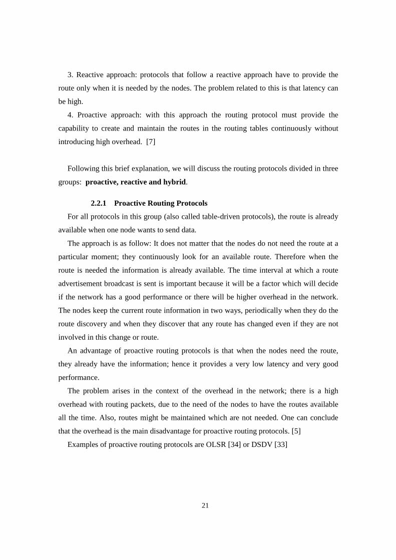
2.2.1 Proactive Routing Protocols
For all protocols in this group (also called table-driven protocols), the route is already
available when one node wants to send data.
The approach is as follow: It does not matter that the nodes do not need the route at a
particular moment; they continuously look for an available route. Therefore when the
route is needed the information is already available. The time interval at which a route
advertisement broadcast is sent is important because it will be a factor which will decide
if the network has a good performance or there will be higher overhead in the network.
The nodes keep the current route information in two ways, periodically when they do the
route discovery and when they discover that any route has changed even if they are not
involved in this change or route.
An advantage of proactive routing protocols is that when the nodes need the route,
they already have the information; hence it provides a very low latency and very good
performance.
The problem arises in the context of the overhead in the network; there is a high
overhead with routing packets, due to the need of the nodes to have the routes available
all the time. Also, routes might be maintained which are not needed. One can conclude
that the overhead is the main disadvantage for proactive routing protocols. [5]
Examples of proactive routing protocols are OLSR [34] or DSDV [33]
22
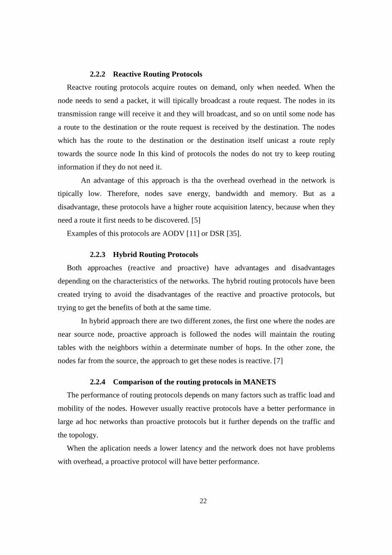
2.2.2 Reactive Routing Protocols
Reactve routing protocols acquire routes on demand, only when needed. When the
node needs to send a packet, it will tipically broadcast a route request. The nodes in its
transmission range will receive it and they will broadcast, and so on until some node has
a route to the destination or the route request is received by the destination. The nodes
which has the route to the destination or the destination itself unicast a route reply
towards the source node In this kind of protocols the nodes do not try to keep routing
information if they do not need it.
An advantage of this approach is tha the overhead overhead in the network is
tipically low. Therefore, nodes save energy, bandwidth and memory. But as a
disadvantage, these protocols have a higher route acquisition latency, because when they
need a route it first needs to be discovered. [5]
Examples of this protocols are AODV [11] or DSR [35].
2.2.3 Hybrid Routing Protocols
Both approaches (reactive and proactive) have advantages and disadvantages
depending on the characteristics of the networks. The hybrid routing protocols have been
created trying to avoid the disadvantages of the reactive and proactive protocols, but
trying to get the benefits of both at the same time.
In hybrid approach there are two different zones, the first one where the nodes are
near source node, proactive approach is followed the nodes will maintain the routing
tables with the neighbors within a determinate number of hops. In the other zone, the
nodes far from the source, the approach to get these nodes is reactive. [7]
2.2.4 Comparison of the routing protocols in MANETS
The performance of routing protocols depends on many factors such as traffic load and
mobility of the nodes. However usually reactive protocols have a better performance in
large ad hoc networks than proactive protocols but it further depends on the traffic and
the topology.
When the aplication needs a lower latency and the network does not have problems
with overhead, a proactive protocol will have better performance.
23
However, if the network suffers from high traffic flow, performing route discovery
with a proactive protocol could be a bad idea because the overhead of route discovery
have a negative effect.
2.3 AODV-UU
2.3.1 Introduction to AODV-UU
AODV-UU is a version of AODV (Ad Hoc On Demand Distance Vector) routing
protocol implemented by Uppsala University (Sweden). AODV-UU implements all
mandatory and some of the optional functionalities of AODV with added functionality of
gateway discovery and half tunneling capabilities. [8]
AODV-UU is an On Demand routing protocol and thus only initiate a Route
Discovery when needed. [5]
2.3.2 AODV Operation
AODV introduces the concept of routing tables in reactive protocols. It keeps
information on destination node information, next hop and the sequence number in order
to find the newest route to the destination in the routing table. [11]
2.3.2.1 Route Discovery
When a node wants to send a packet, the first step is to check if there is an entry for
the destination in the routing table. If there is no entry in the routing table, the node starts
a route discovery phase by sending a RREQ message by broadcast. The RREQ message
consists of the following information: source IP, destination IP, source sequence number,
destination sequence number, the broadcast identifier (to avoid the problem of duplicate
packets in broadcasting) and the time to live (TTL). All the nodes that receive the RREQ
packets check if they have any packet with the same identifier, if they do, they will
discard the packets to avoid duplicate packets. When receiving a non duplicate packet the
nodes create a back way pointer towards the source.
When the destination node receives the RREQ, it sends a RREP to the source node by
unicast in the reverse path.

24
When the route is established, the source node will update the routing table, the
destination node also does the same if the sequence number of the packet is higher than
the one it is in the route tables.
AODV protocol also has an optional Hello Messages mechanism. That means, nodes
sent periodically Hello messages to the neighbors in order to keep connectivity.
When a route is broken, the failure can result from two the movement of the source
node, from the movement of the destination node or from the movement of intermediate
nodes.
If the failure results from the movement of the source, it can start a new route
discovery. However, if the failure results from the movement of the destination or the
intermediate nodes, a special kind of Route Reply message (Route Error) is used to
inform other nodes along the route and the source node of the broken route. The broken
link is always detected by an upstream node, which is the responsible for initiating the
RouteError message. When the source receives the message, it can reinitiate the route
discovery. [13]
The main advantage of this protocol is that routes are discovered on demand; however
time information is stored in the source node routing table. The sequence numbers are
used to find the newest route. [12]
2.3.2.2 Gateway discovery
As mentioned earlier, the AODV-UU is a version of AODV which adds two new
functionalities namely gateway discovery and tunneling.
Gateways are the only way to provide internet connectivity to a MANET. However
the quality service is affected adversely when the MANET has multiple gateways.
When the node needs to send a packet to a wired node or to a node located outside the
MANET, for example in the internet, the mobile node sends a message to request for a
gateway. When the gateway receives this request, it will replay by unicast with a
GWADV. If the node receives more than one gateway advertisement, the node will
choose the gateway it will use depending for example on the number of hops. [7] [13]
25
Tunneling
Each node connected to internet needs a unique IP address; it is used for identification
and even more important, to route the packets to this node. The problem of locating
mobile nodes from an external network in a mobile domain arises because there is not a
centralized organization to assign an unique IP address, so the gateways translates the
hierarchical addressing in IP addresses.
Tunneling is used to solve the problem of sending packet outside the MANET. But
AODV-UU does not use tunneling; it has a new tunneling approach called half-tunneling.
Half –tunneling is a new approach implemented by Uppsala University. It is called
half-tunneling because it only uses tunneling in one way of the data communication. The
tunneling is used only from the source node until the gateway in the MANET.[11]
When a node wants to send a packet, when the node knows that the destination is not
in the MANET, it is achieved with the destination address, the packet (which has the
destination-address of the node outside the MANET) will be encapsulated via a half-
tunneling mode and it will have a new destination address, the gateway address. The
packet will be routed based on the route IP-tunneling header through standard AODV-
UU towards the gateway. The packet will finally be received by the gateway, and it is
then decapsulated at the gateway. It is then sent to the original destination address in the
internet. The tunneling thereby creates a virtual way of one hop between the source and
the gateway. Only the source and gateway know that the encapsulated packets are sent to
a wired node. Therefore the intermediate nodes will not have to look up many times in
routing table because they already know the route to the gateway.
Wired nodes don’t have any problem in sending back packets to the MANET nodes,
they are sent via wired routing towards the gateway. In Ad-Hoc networks, the gateway
which has the same prefix as the mobile node receives the packet directly to send to the
mobile node through standard AODV-UU mechanisms without tunneling. [12]

26
2.4 SIP (session initiation protocol)
2.4.1 Introduction
SIP is the Internet Engineering Task Force's (IETF's) standard for multimedia session
signalling over IP. It is a signaling protocol whose functionality is to set up, control and
tear down multimedia sessions between clients over a network. It can work over a local
network or over the internet. [16]
Session Initiation Protocol was developed by IETF Multi-Party Multimedia Session
Control Working Group known more commonly as MMUSIC. Version 1.0 was given as
an Internet-Draft in 1997.[18]
The session type can serve for several purposes. Usually it is for conferences, but it
can also be used to set up games or video sessions. In general it can be used to set up any
kind of session. SIP is independent of the kind of transport protocols. The data transfer
between the end nodes is independent of SIP and usually based on RTP/RTCP.
SIP is an application-layer protocol. Its functionality can create, modify and tear down
a session, because session management has the ability of controlling an end-to-end call. It
provides the following functionalities:
- Address resolution: It provides the location of the end point.
- Lowest session capabilities: The caller user indicates to the called node when it
sends the invitation which the lowest characteristic of the media session can be
supported. The caller nodes send the maximum characteristics in terms of quality, for
example.[19]
- Set up session between end nodes. It sets up the session if all the steps involved
are correct. If one end node is busy or unreachable, SIP informs the caller node.
- Termination of calls. It handles the termination of calls as well. [18]

27
2.4.2 SIP components
2.4.2.1 SIP Users
A SIP end device is called SIP user, for example cell phones, PCs, PDAs, etc. A SIP
user is a logical device, which has User Agents (UAs). Each SIP user has a SIP User
Agent Client (UAC) and a SIP User Agent Server (UAS).
Each SIP user has an unique identifier, or user name which gives a globally reachable
address. Callees bind to this address using the SIP Register method. Callers use this
address to establish communication with callees. The address is a URI, which can be:
sip:[email protected]. Non SIP-URIs can be used as well, for example mail:,
http:…
-SIP User Agent Client: it is the part of the User Agent which initiates the SIP request.
It works on behalf of the user when it wants to send a request.
-SIP User Agent Server: it is the part of the User Agent which responds to the SIP
requests. It works on behalf of the user when it has to respond to the SIP requests.
[18][17]
2.4.2.2 SIP servers
The SIP servers are the workhorses of the SIP structure. They are the entities which
manage all the SIP messages.
The SIP servers can act as different entities:
-SIP proxy server: usually there is one proxy in each SIP domain for handling
incoming invitations. For instance, if sip:[email protected] sends an invitation to
contact sip:[email protected], the proxy for the domain university.com will receive
the requests of the user Alice and sends the invitation to user Bob. It is the entity
responsible for the users within a domain. [19]
-SIP redirect server: The redirect sever gives back the information about the called
party’s address. This functionality may be neccesary in different situations. The simplest
case is that one in which the caller receives the address of the called party, so that it can
send the SIP messages directly to the called party.
But usually the redirect server provides to the caller the information of other SIP
proxy server. It may happen when, for example, a user may be in different domains when
28
at working place or when at home. The redirect provides the caller information about
alternative addresses to reach the callees, and the next hop to the alternative server in
other domain. [19]
-SIP register server: This is a server which accepts register requests and stores the
information of the user who wants to register in a database called “location service”. It
keeps the information of the users within a domain or a set of domains. When the users
are registered, the information is available to other proxies in the same group of domains.
That means, if [email protected] wants to contact with [email protected] , the information
of Bob will be available for the proxy university.com, so when Alice wants to initiate a
session with bob, the university.com domain proxy will have the information of Bob in
kau.se. [19]
The location service (register server) and the register proxy can be co-located in the
same machine or can be located at different machines. Also the location service can be a
database in the same server or in other. The register, redirect and proxy server can access
to the database with any technology as for example, LDAP; independent of SIP. [17]
29
2.4.3 How SIP works
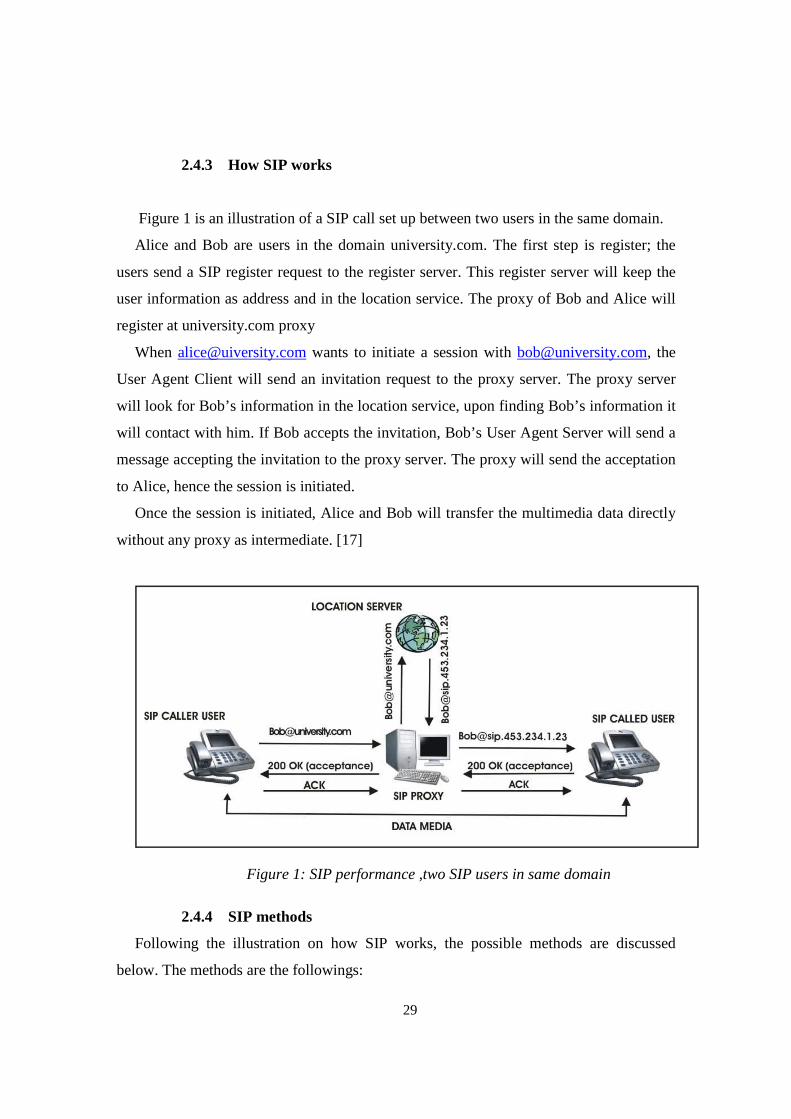
Figure 1 is an illustration of a SIP call set up between two users in the same domain.
Alice and Bob are users in the domain university.com. The first step is register; the
users send a SIP register request to the register server. This register server will keep the
user information as address and in the location service. The proxy of Bob and Alice will
register at university.com proxy
When [email protected] wants to initiate a session with [email protected], the
User Agent Client will send an invitation request to the proxy server. The proxy server
will look for Bob’s information in the location service, upon finding Bob’s information it
will contact with him. If Bob accepts the invitation, Bob’s User Agent Server will send a
message accepting the invitation to the proxy server. The proxy will send the acceptation
to Alice, hence the session is initiated.
Once the session is initiated, Alice and Bob will transfer the multimedia data directly
without any proxy as intermediate. [17]
Figure 1: SIP performance ,two SIP users in same domain
2.4.4 SIP methods
Following the illustration on how SIP works, the possible methods are discussed
below. The methods are the followings:
30
2.4.4.1 INVITE
This method is initiated by the caller user when he wants to invite a callee for a
session. The caller sends a invitation message which includes information with the
session description in the message body. The information about the session may indicate
the lowest characteristic of the media session. The caller tells the called node which is the
lowest media session can be established in terms of quality for example.
2.4.4.2 REGISTER
When a user wants to register, this method sends the information of the user, as the
address, location and other important information in the Location Server. This
information will be available for the server proxy in the same domain.
2.4.4.3 ACK
This method acknowledges the final state of the invitation method, only for invitation
method. That means that the caller user gets a message with the final state for the Sip
invitation.
2.4.4.4 CANCEL
This method is used to terminate an attempt of a SIP call. It is important because if one
user wants to initiate a session with another user, while the Sip invitation is not finished,
the Sip users are in the “Busy” state, in which they can not be contacted with them.
Therefore, if the users decide not to initiate the Sip call, it can be stopped this method.
2.4.4.5 OPTIONS
With this method, a user can ask to another user or to a proxy for their capabilities or for
their availability. This method can not be generated by a proxy server.
2.4.4.6 BYE
This is the method used to terminate the Sip session. It has the particularity that the
message does not go through the proxy. When a user wants the call to finish, he will send
a bye request to the other user. [18]
31
2.4.5 SIP message codes
The following Sip message codes are in part of SIP response messages. The SIP
response messages are the messages that the User Agent Server or SIP servers generate to
reply to a request sent by the User Agents Client. The codes are numbers of three digits.
Depending on the function of the code, it start with 1, 2, 3, 4, 5 or 6. For example, when
the code starts with 1, the message is informational, however when the code starts with 2,
the messages indicate success actions.
These codes reveal how SIP works in the messages exchange between users and SIP
proxy.
The first 5 groups of messages are borrowed from other protocols as Http, only the
group 6 is explicitly implemented for use in Sip protocol. [20] [18]
The most important codes used in the SIP protocol, can be divided into the following
groups:
2.4.5.1 1xx messages: Informational
This range of codes is used to inform about one step in an action.
For example:
-100 code is used to inform the caller that the proxy received the invitation request and
that it has forwarded the invitation to the called party.
-180 code is a message sent by the called party before the acceptance of the invitation is
sent. It sends a 180 message to inform the other party that the SIP invitation has been
accepted and the called party is getting ready to connect.
2.4.5.2 2xx messages : Success
In this class the main code is 200, which is called 200 OK. This message is used to
indicate that a request has been accepted. When this message is used after the invitation
or options methods, it will contain a message body with the media properties or with the
capabilities. If the 200 ok is used for the methods CANCEL, REGISTER or BYE
methods, the message has no body, it is just to indicate that the method has succeeded.
2.4.5.3 3xx messages : Redirection
The 3xx messages are generate by the user to respond to a user invitation request when
the server is acting as a redirect server.
32
The server may act as a redirect server because of many situations and the messages
indicate to the user the reason.
-300 code: This message contains multiples choices. In this message there will be
some addresses to contact with the called party, because the location information of the
called node is not in this proxy. The user agent can be pre-configured to contact with the
new addresses without interact with the user.
-301 code: This message is called “permanently moved”, and it contains a new URI to
contact the called party with. The new address will be used for the future, because the
called party has moved permanently.
-302 code: Temporally moved. This message will contain an address to contact with
the called party, but the address will not be saved because next time, the caller will use
the old address.
-305 Use proxy. This message contains the address of another proxy server which
have the information of the called party.
2.4.5.4 4xx messages : Client error
Client error messages are messages that indicate that an error occurred in the SIP
interaction process which is a result of an error in a user node.
-401 code: This code indicates that the user did not perform the authentication. It is
usually sent by the users, but it can be generated by the servers as well. For example, the
register server can generate this message if the credentials of the user who wants to
register are not correct.
-404 code: Not found. This message is generated by the server when the URI of the
user does not exist or it is not register in any server.
-408 code: Request timeout. This message is generated when the time of the session
set up was expired.
-486 code: Busy . This message is generated when the user receives an invitation but it
is already in the “busy” state. For example, after the user sends an invitation or receives
an invitation, its state will change to busy state until the SIP session is finished. So no
other user can try to invite this user during this time.
33
2.4.5.5 5xx messages: Proxy error
These messages are generated because the server can not process any requests. The
requests can then be resent to another server, because there is no problem with the
request.
-500 code: Server internal error. This message indicates that there is some kind of
internal error with the server.
-502 code: Bad gateway. This message is generated by a proxy server which is acting
as a gateway to another network and tells that some problem in the other network is
preventing the request from being processed.
2.4.5.6 6xx messages: Global failure
This group of messages is generated by the server. The server knows that the request will
fail.
-600 code: Busy everywhere. This is a version of the error 486, but the server already
knows that the user state is busy.
-606 code: Decline: This message results in a similar action as the last message (600),
but in this one, one does not know why the invitation is declined. It may because the user
is busy or simply it does not want to accept a request. [20] [18]

34

35
3 Network Simulator 2
This chapter describes Network Simulator 2, used in this master´s thesis.
The chapter is structured as follows:
Section 3.2 explains how to write and to structure a Tcl script. Section 3.3 explains
what class node is and how it works internally. Section 3.4 describes Network Simulator
Link class along with how it works internally and how it interacts with other classes.
Section 3.5 describes class Packet. Section 3.6 describes agents class. It contains the
goals and functionalities of these agents and their interactions with the packets. Section
3.7 explains how to choose the radio propagation model. How to choose among existing
different radio propagation models; depending on some parameters is explained in this
section. Section 3.8 describes how to calculate the communication range to use in the
simulations. Using some parameters, a tool in Network Simulator called “threshold” is
used to configure the communication range. Section 3.9 explains how to describes how to
configure wireless and wired network simulators.Section 3.10 describes the trace files.
3.1 Introduction
The Network Simulator 2 is an object-oriented, discrete, event-driven network
simulator. It is implemented in OTcl and C++. Using two different programming
languages is not so usual in applications, but it has some advantages. A major advantage
of this feature is that it makes it possible for users to write the simulation scripts in Tcl1
(due to NS is an object-oriented Tcl script interpreter).
More complex functionalities based on C++ can be added by the user. This flexibility
is very important to enhance the simulation environment that is needed. The most
common components are built in the simulator, for example wired nodes, wireless nodes,
links, agents and applications. The Network Simulator 2 also uses C++ for efficiency
reasons. The NS libraries are written in C++ (Event Scheduler Objects, Network
Component Objects, Network Setup Helping, Modules) [23]. Many network components
1 It is easier to write scripts in Tcl

36
can be configured in detail. Also traffic patterns can be added to give more reality to the
simulations.
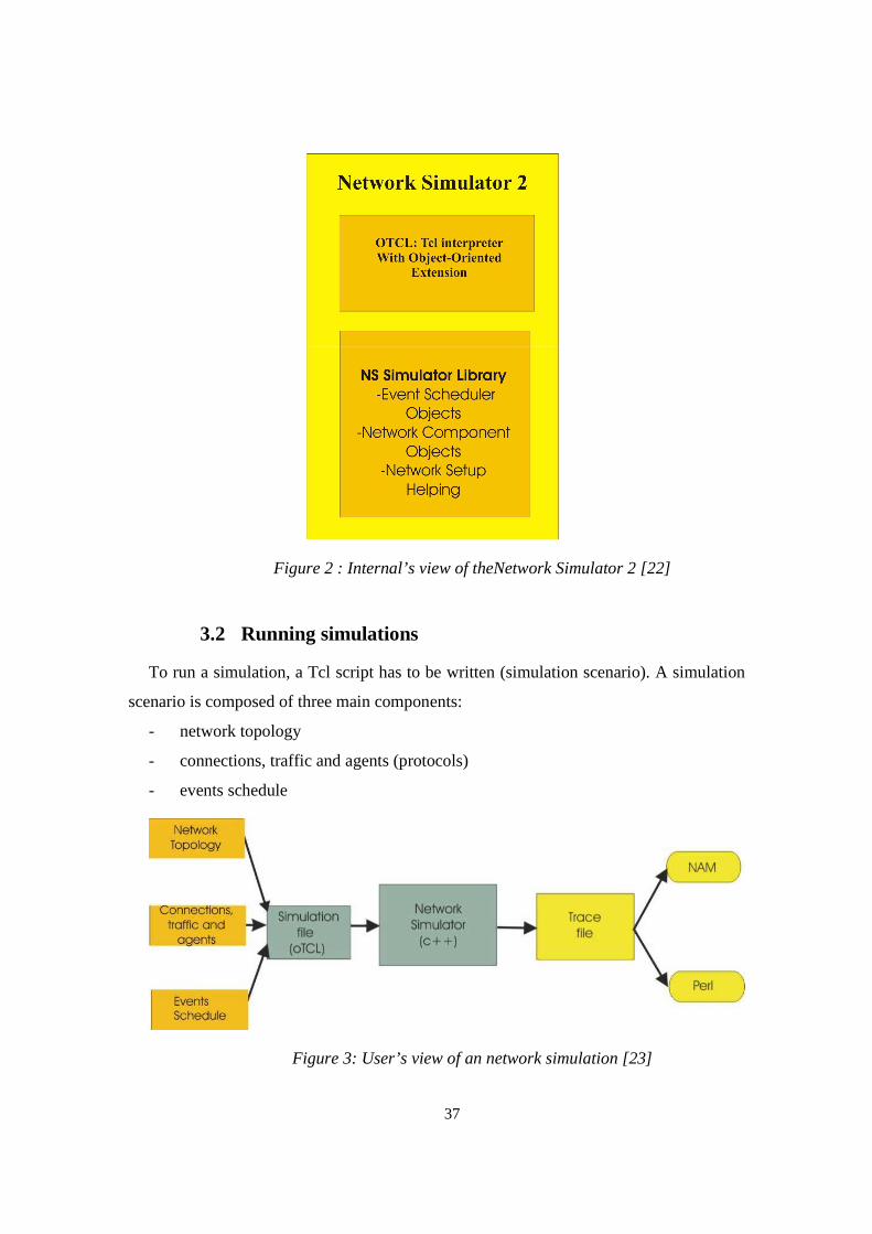
As depicted in Figure 2, the Network Simulator 2 can be seen structured in two very
different parts; the Tcl interpreter and the NS Simulator Library. Figure 3 shows the work
flow in the simulation when the user uses the Network Simulator 2 to run simulations.
The user writes a Tcl script (structured in three different parts as network topology,
connections, traffics and agents and events schedule) to define the total scenario to be
simulated. Such a script is interpreted by the Network Simulator 2 using C++ classes
(agents, links, packets, queue… etc).
After running the simulations, the Network Simulator 2 gives out a trace file showing
the trace information about all the information requested for in the Tcl script. There are
different approaches to interpreting a trace file; the most common approaches are:
- NAM (network animator): It is a program that graphically shows the packets and
how the traffic flows behave.
- Perl (programming language): used to extract the information. It is a very good
programming language for this function due to the facility to work with data and
strings. It is very useful for extracting data and printing it out in other files or
formats in order to study them or to plot them in graphs.
37
Figure 2 : Internal’s view of theNetwork Simulator 2 [22]
3.2 Running simulations
To run a simulation, a Tcl script has to be written (simulation scenario). A simulation
scenario is composed of three main components:
- network topology
- connections, traffic and agents (protocols)
- events schedule
Figure 3: User’s view of an network simulation [23]

38
A network topology defines the scenario in terms of number of nodes and the
connectivity between them. When the simulation script is built, usually it follows a
certain pattern consisting of the following items:
- Simulation network instance
The simulation instance has to be defined in every simulation. The simulator object is
generated and it is assigned to the variable ns. See Code 1.
..Creating object simulator instance...
set ns [new Simulator]
Code 1: simulator instance
What this line does is that it initializes the packet format creates a schedule and selects
the default address format [22].
- Opening trace files
The trace files and their formats that we want to receive as an output is defined here. It
can be the normal NS trace file or the NAM trace file. See Code 2.
...Opening the trace files...
set nf [open trafileName.tr w]
$ns trace-all $nf
Code 2: Opening trace files
- Configuration of nodes
The node settings are defined. The nodes will have all the settings defined when they
are created. Section 4.3.1 explains with examples how to configure wireless and wired
nodes.
- Creation of nodes and links
The nodes are created; they will have the settings defined in above point. The links
between the nodes will be established if the nodes are wired. If the nodes are wireless, the
connection settings are already defined in above point “configuration nodes”. Section
4.3.1 explains with examples how to create the nodes and to link them.
39
- Creation of agents and applications
At this point the agents (protocols) are attached to the nodes to create application
events. Section 4.3.2 explains with example how to create agents and applications.
- Events schedule
The time events are defined, when the events start and when they finish. Section 4.3.3
shows how to implement it in Tcl scripts.
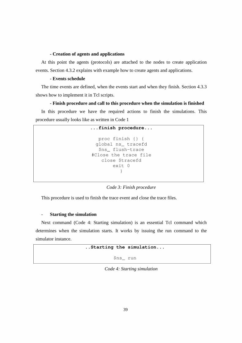
- Finish procedure and call to this procedure when the simulation is finished
In this procedure we have the required actions to finish the simulations. This
procedure usually looks like as written in Code 1
...finish procedure...
proc finish {} { global ns_ tracefd
$ns_ flush-trace #Close the trace file
close $tracefd exit 0
}
Code 3: Finish procedure
This procedure is used to finish the trace event and close the trace files.
- Starting the simulation
Next command (Code 4: Starting simulation) is an essential Tcl command which
determines when the simulation starts. It works by issuing the run command to the
simulator instance.
..Starting the simulation...
$ns_ run
Code 4: Starting simulation
40
3.3 Node structure
Nodes are fundamental in NS-2 and in the simulations. They are the most important
entities in the simulations; they perform processing and forwarding of packets. In this
section, two different objects are described, namely the internal structures of wireless and
wired nodes.
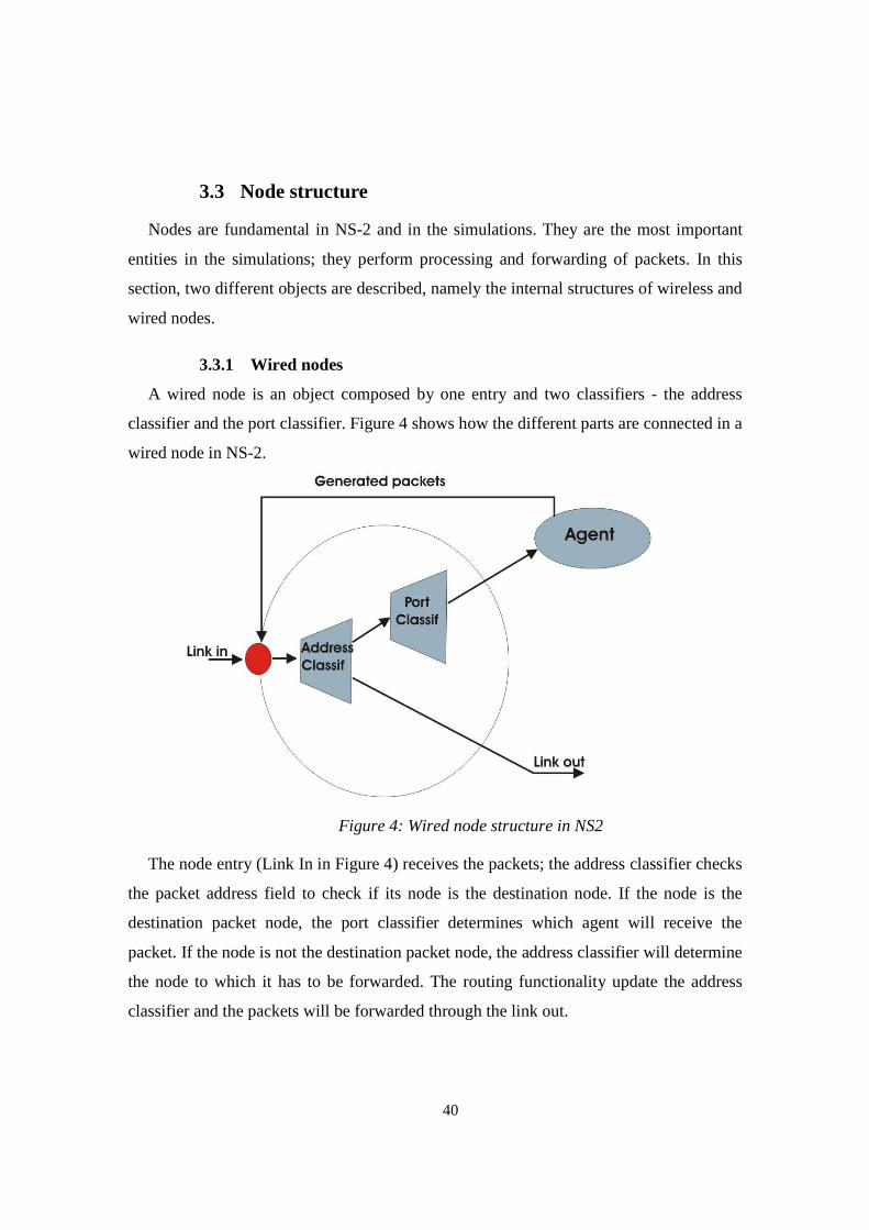
3.3.1 Wired nodes
A wired node is an object composed by one entry and two classifiers - the address
classifier and the port classifier. Figure 4 shows how the different parts are connected in a
wired node in NS-2.
Figure 4: Wired node structure in NS2
The node entry (Link In in Figure 4) receives the packets; the address classifier checks
the packet address field to check if its node is the destination node. If the node is the
destination packet node, the port classifier determines which agent will receive the
packet. If the node is not the destination packet node, the address classifier will determine
the node to which it has to be forwarded. The routing functionality update the address
classifier and the packets will be forwarded through the link out.

41
3.3.2 Wireless nodes
In this section, the wireless node structure in the Network Simulator 2 is described.
Figure 5 shows the internal work flow of wireless nodes.
The node always receives the packets at the node entry. The packet goes through the
address classifier where its address field is examined. The agents are connectors. When
the connectors receive packets, they execute some functions and deliver the packets to
their neighbors or drop them. There are different types of connectors performing different
functions, e.g., Agent, Link Layer, MAC Layer and Network Interface. The interaction
between them is shown in Figure 5.
Figure 5:Wireless node structure in NS2
42
3.4 Links
How the nodes are linked is described next. The following Tcl script shows how a link
is created.
..Definition of link in Tcl...
$ns <link_type> <node0> <node1> <bandwidth> <delay> <queue_type >
Code 5: Link definition in a Tcl script
The parameters needed for a link definition are:
-link_type: this parameter specifies the type of link is used between the nodes (node1
and node0)
-bandwith: this parameter specifies the bandwidth of the link.
-delay: this parameter is a number, which defines in milliseconds the link delay.
-queue_type: the link use queue_type performance mode.
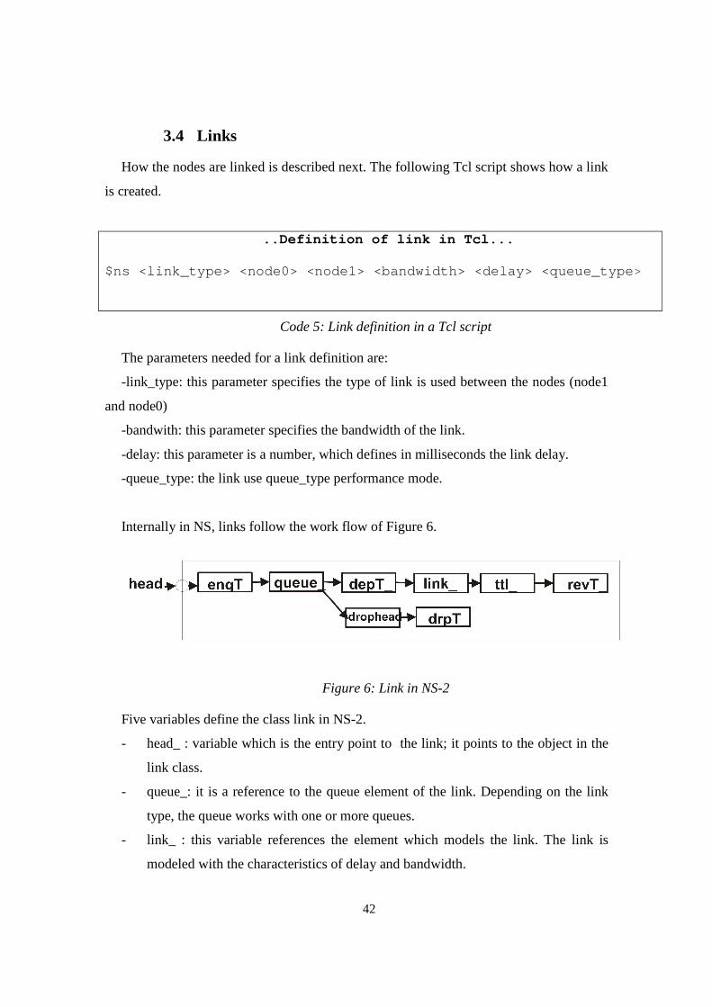
Internally in NS, links follow the work flow of Figure 6.
Figure 6: Link in NS-2
Five variables define the class link in NS-2.
- head_ : variable which is the entry point to the link; it points to the object in the
link class.
- queue_: it is a reference to the queue element of the link. Depending on the link
type, the queue works with one or more queues.
- link_ : this variable references the element which models the link. The link is
modeled with the characteristics of delay and bandwidth.
43
- ttl_: this variable points to the element which works with the ttl (time to live) of
every packet.
- drophead_: this variable makes reference to an object which is the element that
processes the link drops.
In addition, there are instance variables defined in the link class to trace the link
events. These elements are:
- enqT_ : traces packets that enter in queue_.
- deqT_ : traces packets that leave queue_.
- drpT_ : traces packets that are dropped from queue_.
- revT_ : trace packets that are received in the next node.
3.5 Packets
After nodes, packets are the most important objects in simulations. A packet is
composed by a packet header and a packet data.
The packet headers are added by protocols when the packet goes through the different
layers. The only packet header that is obligatory is called the common header. The
common header is used to trace the packet and to calculate or measure other parameters
during the simulation. The structure of a packet is shown below in Figure 7.

44
Figure 7: Packet structure in NS-2
The size of the packet is defined in compilation time, at the startup of the simulation.
The packet contains information about next packet and the size of the header (hdr_size).
The packet header contains the headers of many protocols and the common header
which contains information about the packet.
Some of the most important fields in the common header are commented on below:
- ptype : the type of the packet.
- size : the size of the packet.
- uid_ : unique identifier for the packet
- error_ : this field is activate if the packet contains any error.
- errorbitcnt_: identifies the bits that contain the error.
- direction_: this field contains which is the direction in which the packet follows in
the simulation transversal.
- prev_hop_ : this field indicates the last hop where the packet come from.
- next_hop_: this field indicates the next hop where the packet goes.
- num_forwarders_: used in wireless simulations, contains how many times a
packet has been forwarded.
- iface_: the label of the link which received the packet.

45
3.6 Agents
Agents simulate end points where packets are created or received. They are used to
implement the protocols at various layers.
Agents hold state information, mainly to be able to assign default values to packet
fields when generating packets and identifying itself. The state information which they
hold is the following:
Variable Description agent_addr The address of this agent agent_port_ The port number of this agent dst_addr_ The address of the destination agent dst_port_ The port number of the destination agent
type_ The packet type size_ The packet size ttl_ The time to live of the packets fid_ The IP address flows identifier
prio_ The IP priority field
Table 1: Agent state information
Agents are used to simulate protocol behavior. The agents are attached to the nodes.
The agent will receive the packets destined for it, that means, all the packets whose port
number is the port of the agent.
Routing agents are special cases of agents. They need more steps in order to be
installed in the nodes. Agents are created in Tcl, and the default values of the agents can
be modified in Tcl code during creating.
Agents are attached to the nodes by issuing: attach-agent <node><agent>. To allow
two agents attached to different nodes to communicate, the Network Simulator 2 instance
offers a connect <src><dst> command to connect them to each other. In such a case, it
is necessary to have the nodes to which the agents are attached, connected by a link.
To simulate traffic, two agents need to be created and attached to the source and
destination nodes. Source and destination nodes can be located in wired or wireless
network.

46
3.7 Radio Propagation Models
In NS-2 there are three propagation models: free space model, two-ray ground
reflection model and the shadowing model. Their implementations in NS-2 are done
using the following files:
- for free space model: ~ns/propagation.{cc,h}
- for two-ray ground reflection model: ~ns/tworayground.{cc,h}
- for shadowing model: ~ns/shadowing.{cc,h}
Shadowing Model is discarded due to the simplicity of the simulation. In order to
choose the optimum of the two remaining propagation models for our simulations, we
need to calculate a cross-over distance.
When the distance between transmitter and receiver, d, is less than the cross-over
distance, dc (d < dc), the free space model is used. Otherwise when d > dc two ray
ground model is used.
The cross-over distance is calculated as
λπ hrhtdc ××= 4 (1)
Where:
- λ is the wavelength.
- ht is the height of transmitter antenna
-hr is the height of receiver antenna
According to two ray ground model, the distance d can be calculated given the
received power of the mobile node. Transmission power is 100mW, the transmitter and
receiver antenna gain are 1, the system loss, L is and the transmitter and receiver antenna
height are 1,5 meter.
Therefore, calculating the eq.2, we obtain a value of d > dc. [30]
( )Ld
hhGrGtPtd rt
×××××= 4
22
Pr (2)
Where:
-Pr(d): received signal power at d distance
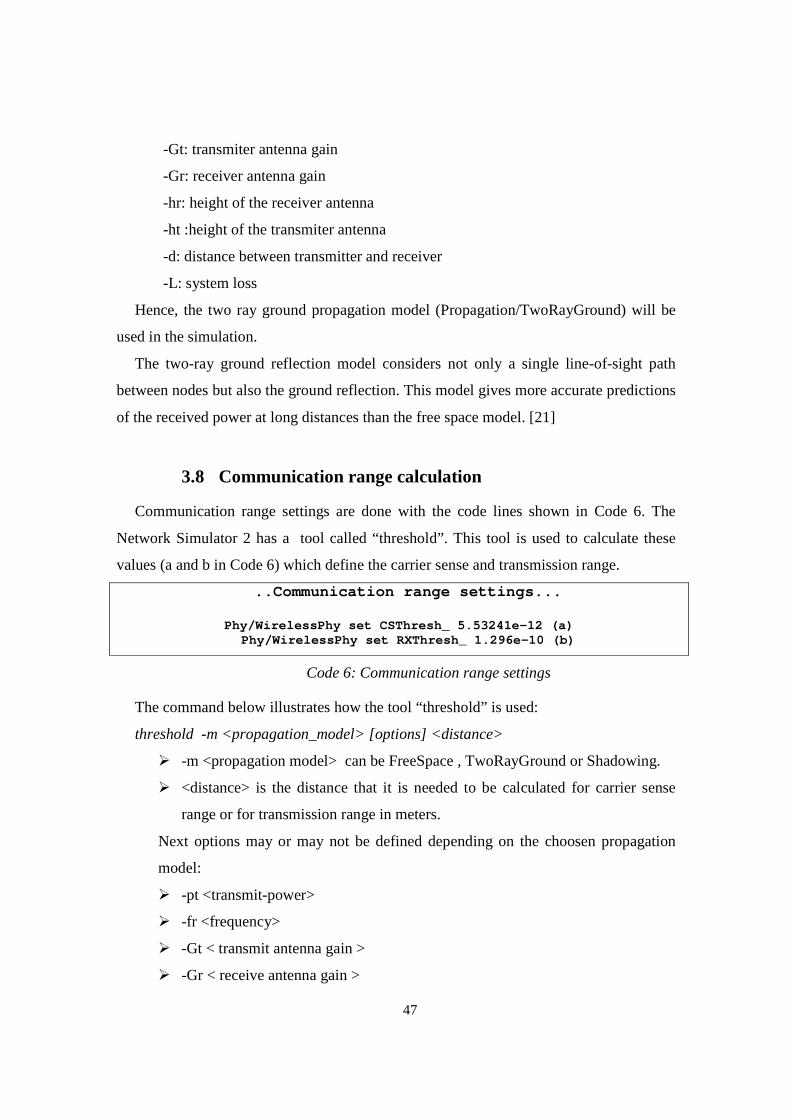
47
-Gt: transmiter antenna gain
-Gr: receiver antenna gain
-hr: height of the receiver antenna
-ht :height of the transmiter antenna
-d: distance between transmitter and receiver
-L: system loss
Hence, the two ray ground propagation model (Propagation/TwoRayGround) will be
used in the simulation.
The two-ray ground reflection model considers not only a single line-of-sight path
between nodes but also the ground reflection. This model gives more accurate predictions
of the received power at long distances than the free space model. [21]
3.8 Communication range calculation
Communication range settings are done with the code lines shown in Code 6. The
Network Simulator 2 has a tool called “threshold”. This tool is used to calculate these
values (a and b in Code 6) which define the carrier sense and transmission range.
..Communication range settings...
Phy/WirelessPhy set CSThresh_ 5.53241e-12 (a) Phy/WirelessPhy set RXThresh_ 1.296e-10 (b)
Code 6: Communication range settings
The command below illustrates how the tool “threshold” is used:
threshold -m <propagation_model> [options] <distance>
� -m <propagation model> can be FreeSpace , TwoRayGround or Shadowing.
� <distance> is the distance that it is needed to be calculated for carrier sense
range or for transmission range in meters.
Next options may or may not be defined depending on the choosen propagation
model:
� -pt <transmit-power>
� -fr <frequency>
� -Gt < transmit antenna gain >
� -Gr < receive antenna gain >

48
� -L <system loss>
� -ht < height of the transmitter antenna >
� -hr < height of the receiver antenna >
3.9 Wired cum wireless simulation
The Network Simulator 2 can be used to run simulations modeling many scenarios. It
can work with many applications, protocols and it can simulate wireless, wired and
wireless-cum-wired scenarios. Wired cum wireless simulation scenarios will be explained
in this section. So far, the configuration of the nodes was not so complicated, its
complexity increases a little bit when we run a simulation with wireless and wired nodes
simultaneously. [21]
When a wired network is connected with a wireless network, base stations are needed
to act as interfaces between the networks. Base stations are like gateways, they permit
packets to be exchanged between different kinds of nodes.
Hierarchical addresses are needed in nodes to route packets between wireless and
wired domains. It is not necessary to have different domains for wired and wireless
nodes; the wireless nodes will be in the same domain as the gateway which will be the
home gateway (the gateway which is the predefined gateway for them). If these mobile
nodes change position and they go near other base stations, mobile IP will solve the
addressing problem. The gateway has to be connected with the wired nodes as well.
If the nodes have mobility in the simulation, we have to define one gateway as the
home agent for the nodes which are predefined for this gateway. Foreign agents are
gateways outside of the domain.
3.10 Trace file structure
The result or output of running a simulation is the trace file. The trace file is a file with
special formats which returns the information of all packets that have flooded through the
network during the simulation. This information will be variable depending on the
options that are defined in the simulation Tcl file.

49
Depending on which information you want to trace, there are different levels or layer
to trace, for example if we want trace the routing packets, if we want to trace the Mac
layer packets.
There are two different trace formats: old and new trace wireless formats. In this
dissertation, old trace format is used. The new trace format gives more information about
the packets, but old trace format information is enoutgh for us.
Some different kinds of trace packet information can be received depending on the
used protocols. All possible trace formats will be mentioned here, but more attention will
be given the cases that we used in our studies.
It is important to differentiate between the trace information of a wired node and a
wireless node. [22] First, the wired format will be discussed.
Wired format
The wired format is very simple and it has always 12 fields.
An example:
- 31.353348 45 0 SIP 250 ------- 0 1.0.57.5 0.0.0.5 -1 10439
Field Pos Field description
1st Event: r: Receive, d: Drop, +: Enqueue, -: Dequeue
2nd Time of the event
3rd Source node Id
4th Destination node Id
5th Packet name or type , it can be exp,Sip…depending on which kind of traffic
6th Packet size
7th Flags
8th Flow id
9th Source address, usually node.port, so last number is the port
10th Destination address: the destination address , with last number being the
port
11th Sequence number that NS gives for any event
12th Unique packet id, all the packets have an unique Id
Table 2: Wired trace format fields

50
In some protocols, additional information about other fields may be available.
However, those are special cases and will not be used in this dissertation.
Wireless format
In wireless trace format, the field choices have to be determined in the simulation
script. It can be mainly of two different formats: old format and new format. The old
trace format is used in our trace files; therefore we will focus on the fields which
compose the old trace file.
In this dissertation we will use only two different types of data packets. They are
Exponential traffic and SIP traffic. Each line below is an example of each data packet
type.
..Example of SIP and Exponential traffic trace lines...
s 35.000 _69_ AGT --- 1103 SIP_INVITE 80 [0 0 0] --- [1.0.23:5 0.0.0:5 32 0] [1] 0 0
s 35.0068 _141_ AGT --- 11035 exp 12 [0 0 0 0] --- [1.0.78:0 1.0.96:0 32 1.0.96]
[536] 4 0
The first twelve fields contain information about the event, the next four contain
information about the IP protocol and the last three contain information about its
corresponding technology as Exponential traffic and SIP traffic.
The below table briefly describes the twelve fields containing information about the
event. [8]
Field Pos Field Description
1st Event: s: sent r: received f: forwarded d: drop
2nd Event time
3rd Node Id
4th Trace name (AGT for agent trace, RTR for routing trace )
5th Reason , usually the reason when a packet is dropped
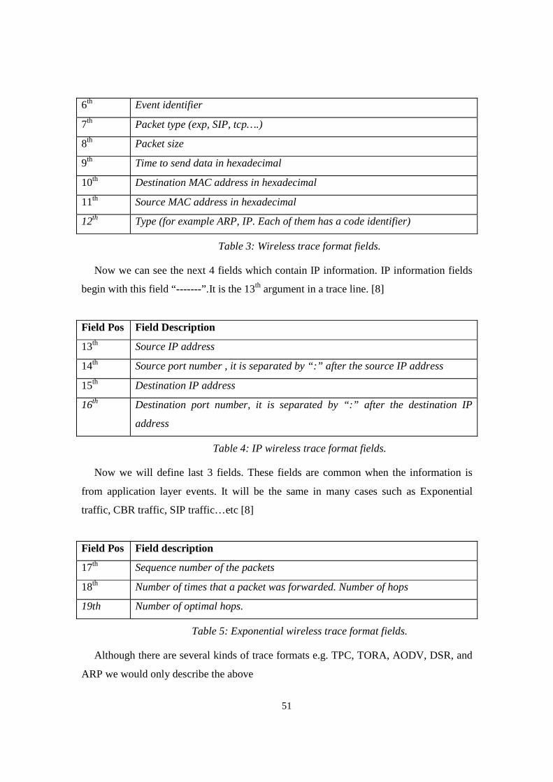
51
6th Event identifier
7th Packet type (exp, SIP, tcp….)
8th Packet size
9th Time to send data in hexadecimal
10th Destination MAC address in hexadecimal
11th Source MAC address in hexadecimal
12th Type (for example ARP, IP. Each of them has a code identifier)
Table 3: Wireless trace format fields.
Now we can see the next 4 fields which contain IP information. IP information fields
begin with this field “-------”.It is the 13th argument in a trace line. [8]
Field Pos Field Description
13th Source IP address
14th Source port number , it is separated by “:” after the source IP address
15th Destination IP address
16th Destination port number, it is separated by “:” after the destination IP
address
Table 4: IP wireless trace format fields.
Now we will define last 3 fields. These fields are common when the information is
from application layer events. It will be the same in many cases such as Exponential
traffic, CBR traffic, SIP traffic…etc [8]
Field Pos Field description
17th Sequence number of the packets
18th Number of times that a packet was forwarded. Number of hops
19th Number of optimal hops.
Table 5: Exponential wireless trace format fields.
Although there are several kinds of trace formats e.g. TPC, TORA, AODV, DSR, and
ARP we would only describe the above
52
4 Design and Implementation
From this point onwards, attention is focused on discussing the work carried out on the
thesis, including the following approaches to achieve the goals as well as explaining all
the used scripts.
This chapter focuses on the parameters used to get different simulations and different
useful results. These parameters are supposed to be very important to see the performance
and behavior of the Hybrid Ad Hoc Network with the VoIP.
This chapter is structured as follows:
- In section 4.1, the simulation goals are described.
- In section 4.2, the different areas of concern in these thesis studies are described.
- In section 4.3, all the Tcl script code to run the simulations are explained.
- In section 4.4, post-tracing is explained; the information extracted from the trace
files.
- In section 4.5 the performance parameters are described, how to calculate them
having the extracted information from the trace files.
4.1 Introduction and goals
The goal of our simulations is to observe the behavior and to determine the
performance of the Hybrid MANET working in several different situations with VoIP.
A MANET scenario is set up adding several different parameters which will create
many different simulations. The network is a hybrid MANET. It is a MANET that
always has any gateway providing internet connectivity with an external network. The
number and positions of gateways are varied in different simulations.
Some Exponential traffic flows will be created in the network modeling voice
conversations. The number of traffic flows and the distance between sources and
destinations will be varied during the simulations, many SIP call attempt will be initiated
as well.
53
4.2 Areas of concern
In this section, different areas of concern associated with this thesis are described. The
Tcl scripts, Perl scripts and plotted graph parts used in achieving the goal of this thesis
are analyzed.
4.2.1 Tcl Scripts:
As earlier mentioned, a Tcl script is used for parameterizing and configuring
simulations (inside which there are a lot of requirements and functionalities). Tcl scripts
contain the following code:
� Physical and protocol specifications
� Node creation and placement.
� Node communications, with traffic flows, connections and communications.
� Trace, event logs and visualization setups.
4.2.2 Perl Scripts:
Perl scripts are used to manage the information from the trace files generated by
simulations. Some of the uses of the Perl scripts are:
1.- Extracting information from different files.
2.- Calculating certain parameters with information extracted and organized in file(s)
after obtained from the trace files.
3.- Organizing needed information in appropriated format to plot the results in graphs
using a plotting program called “Gnuplot”.
4.2.3 Plotted graphs:
After having the information in the appropriate format, to plot the result graphs is the
last task for obtaining the information to evaluate the simulations.
The graphs are used to examine and compare the results of different simulation
scenarios.
4.2.4 Main contributions
The main contributions of this thesis are listed as follows:
54
- I have studied deeply the routing protocols, much deeper AODV-UU and the
session protocol SIP.
- I have studied and understood the Network Simulator 2 to run all the
corresponding simulations to achieve the goal of this thesis.
- I have designed and implemented several scenarios with varying number of
gateways, number of background traffic flows, distance between sources and
destinations nodes of the background traffic flows, link characteristics, SIP caller
and called nodes, etc..
- I have designed and solved some problems of configuring AODV-UU in the
Network Simulator 2 and how to implement the nodes to act as base stations.
- I have defined properly the approaches to study the performance of the Hybrid
MANETs such as to define the source and destination nodes placement, the
number of traffic flows, the gateways placement, etc..
- I have written several scripts in Perl to extract all the needed information to
compute the performance parameters. I have implemented several scripts to
organize that information to ensure the possibility of comparing the results of the
simulations adding gateways or increasing the number of hops between source
and destinations. I have written some Perl scripts as well to organize the
performance parameters information in an appropriate format for use with
GnuPlot program.
- I have used GnuPlot and Excel to plot several graphs to deeply examine the
behavior of the scenarios in terms of performance parameters.
- I have evaluated and interpreted the results. Some difficulties arose because there
are two kinds of traffic flows; the interpretation of background traffic flows in
general was very difficult, therefore I differentiated when evaluating the inside
background traffic flows and outgoing traffic flows which behave differently, so
evaluating them together is not easy or useful.
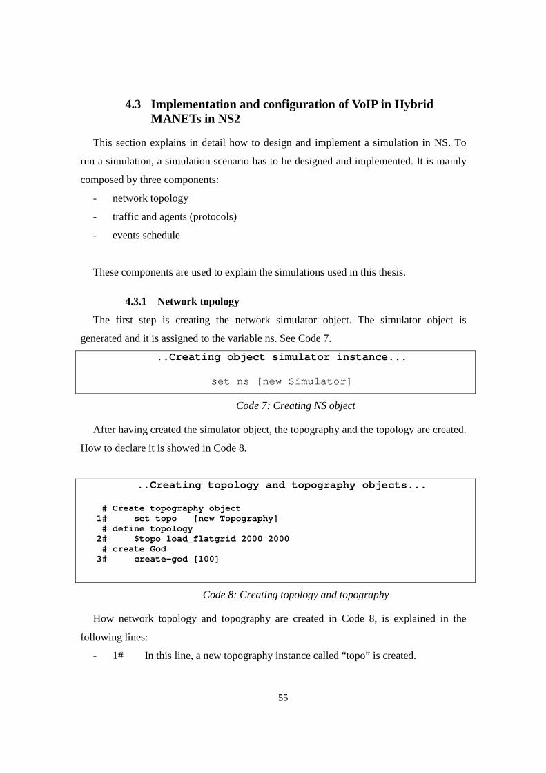
55
4.3 Implementation and configuration of VoIP in Hybrid MANETs in NS2
This section explains in detail how to design and implement a simulation in NS. To
run a simulation, a simulation scenario has to be designed and implemented. It is mainly
composed by three components:
- network topology
- traffic and agents (protocols)
- events schedule
These components are used to explain the simulations used in this thesis.
4.3.1 Network topology
The first step is creating the network simulator object. The simulator object is
generated and it is assigned to the variable ns. See Code 7.
..Creating object simulator instance...
set ns [new Simulator]
Code 7: Creating NS object
After having created the simulator object, the topography and the topology are created.
How to declare it is showed in Code 8.
..Creating topology and topography objects...
# Create topography object 1# set topo [new Topography] # define topology 2# $topo load_flatgrid 2000 2000 # create God 3# create-god [100]
Code 8: Creating topology and topography
How network topology and topography are created in Code 8, is explained in the
following lines:
- 1# In this line, a new topography instance called “topo” is created.

56
- 2# In this line, the new topology instance called “topo” is defined as a flat
grid. Since these simulations are run in a grid of 10 x 10 wireless nodes separated by 200
meters, the flat grip is 2000 meters x 2000 meters.
- 3# This line creates a God instance. The number of wireless nodes is passed
as an argument. It is used to create a matrix to store connectivity information of the
topology.
Since the study is related with Hybrid MANETs with wireless and wired nodes as
components and a special case of wireless nodes called base stations acting as gateways,
they will be explained separately later. Before creating any node, it is important to define
the addressing.
4.3.1.1 Addressing
After creating the topography and topology, the next needed configuration is
addressing. In conventional networks, addressing is set manually or automatically set by
protocols such DCHP.
Addressing is more complicated since a central responsible to manage it does not
exist.
Since there is not mobility in these thesis simulations, it was decided not to use Mobile
IP. Not using Mobile IP creates problems when there are gateways; the solution is to use
different addressing level for nodes. The addressing levels are distributed as follows:
- Wired nodes are in first level. Their addresses are in the format 0.0.x.
- Wireless nodes are addressed depending on the numbers of gateways that exist in
the scenarios. The first important thing is having the gateways in the same
addressing range as the wireless nodes which are supposed to send and receive
packets through that gateway.
- If there is one gateway, all the nodes have 1.0.x as addresses. The same
address level as the gateway.
- If there are two gateways, one gateway is in 1.0.x range and the other is in
2.0.x range. The scenario is divided into two; all wireless nodes which work with
the first gateway (1.0.x) are addressed in the same range, and all the wireless
nodes which work with the second gateway (2.0.x) are addressed in the other
range.

57
- When there are four gateways, the scenario is divided in four groups; each
part has one gateway, so, each gateway and its nodes are in the same address
range.
- Gateway 1 and its wireless nodes: 1.0.x
- Gateway 2 and its wireless nodes: 2.0.x
- Gateway 3 and its wireless nodes: 3.0.x
- Gateway 4 and its wireless nodes: 4.0.x
Alternative approaches
The alternative approach is use Mobile IP. To use Mobile IP, each wireless node has
to be attached to a gateway, which is called “Home Agent”, the other gateways are
“Foreign Agents” for this wireless node. Not using Mobile IP was decided because there
is no mobility in our scenarios.
4.3.1.2 Fixed Nodes
The wired network is connected with the wireless network through the base stations.
The network is a start topology network. The node W(0) is connected with all the other
wired networks. As it was defined earlier, the hierarchical addressing of wired nodes is
0.0.x.
..Creating wired nodes...
set W(0) [$ns_ node 0.0.0]
...
set W(x) [$ns_ node 0.0.x]
..Connecting wired nodes...
$ns_ duplex-link $W(0) $W(1) 5Mb 40ms DropTail
…
$ns_ duplex-link $W(0) $W(x) 5Mb 40ms DropTail
Code 9: Definition and connection of wired nodes

58
The connections between the nodes are duplex-link connections with 5Mb bandwidth
and 40 milliseconds of delay. The queue is Droptail. Duplex-link in NS means that the
procedure “duple-link“ builds a bi-directional simplex-link Droptail queue implements
FIFO scheduling (First In First Out) and drop-on-overflow buffer management.
4.3.1.3 Wireless Nodes
In this point, only the normal mobile wireless nodes are considered, that means, the
special mobile nodes which are acting as gateways called “base stations” would be
explained later. To use wireless nodes in a simulation scenario the Physical layer, the
MAC layer and the mobile nodes declaration have to be considered:
4.3.1.3.1 Physical Layer
As defined for this study, wireless nodes have 550 meters of carrier sense range and
250 meters of transmission range. A tool (~ns/indep-utils/propagation/threshold.cc)is
used to calculate the values (carrier sense threshold and receive threshold). The following
values are needed to make the calculations (how to do it is shown in chapter 3).
• Transmission Rate: 24 mbps (IEEE 802.11g)
• Node spacing: 200 meters
• Carrier Sense Range: 550 meters
• Transmission Range: 250 meters
• Transmission Power = 0,1W (Watts)
• Transmit and Receive Antenna Height: 1,5 meter
• System Loss (L) = 1
• Sensitivity = -85 dBm
After the physical parameters for the simulations are calculated, they are inserted in
the simulation script as follow:
..Physical Layer Parameters...
1# Phy/WirelessPhy set CSThresh_ 5.53241e-12 2# Phy/WirelessPhy set RXThresh_ 1.296e-10 3# Phy/WirelessPhy set bandwidth_ 24Mb 4# Phy/WirelessPhy set Pt_ 0.1 5# Phy/WirelessPhy set L_ 1.0 6# Phy/WirelessPhy set freq_ 2.4e+9
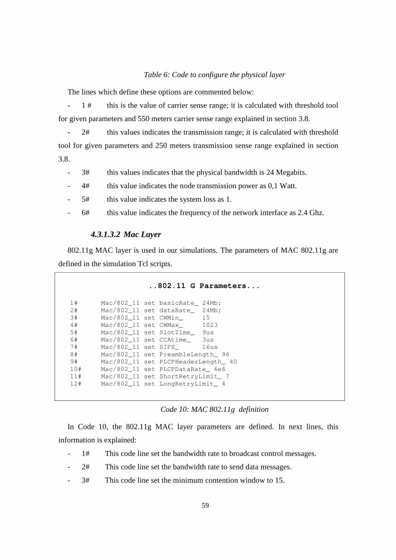
59
Table 6: Code to configure the physical layer
The lines which define these options are commented below:
- 1 # this is the value of carrier sense range; it is calculated with threshold tool
for given parameters and 550 meters carrier sense range explained in section 3.8.
- 2# this values indicates the transmission range; it is calculated with threshold
tool for given parameters and 250 meters transmission sense range explained in section
3.8.
- 3# this values indicates that the physical bandwidth is 24 Megabits.
- 4# this value indicates the node transmission power as 0,1 Watt.
- 5# this value indicates the system loss as 1.
- 6# this value indicates the frequency of the network interface as 2.4 Ghz.
4.3.1.3.2 Mac Layer
802.11g MAC layer is used in our simulations. The parameters of MAC 802.11g are
defined in the simulation Tcl scripts.
..802.11 G Parameters...
1# Mac/802_11 set basicRate_ 24Mb; 2# Mac/802_11 set dataRate_ 24Mb; 3# Mac/802_11 set CWMin_ 15 4# Mac/802_11 set CWMax_ 1023 5# Mac/802_11 set SlotTime_ 9us 6# Mac/802_11 set CCAtime_ 3us 7# Mac/802_11 set SIFS_ 16us 8# Mac/802_11 set PreambleLength_ 96 9# Mac/802_11 set PLCPHeaderLength_ 40 10# Mac/802_11 set PLCPDataRate_ 6e6 11# Mac/802_11 set ShortRetryLimit_ 7 12# Mac/802_11 set LongRetryLimit_ 4
Code 10: MAC 802.11g definition
In Code 10, the 802.11g MAC layer parameters are defined. In next lines, this
information is explained:
- 1# This code line set the bandwidth rate to broadcast control messages.
- 2# This code line set the bandwidth rate to send data messages.
- 3# This code line set the minimum contention window to 15.

60
- 4# This code line set the maximum contention window to 1023.
- 5# This code line set the slot time for back-off window to 9µs.
- 6# This code line set the CCAtime to 3µs.
- 7# This code line set the short interframe space (SIFS) to 16 µs.
- 8# This code line sets the length of the preamble to 96 bits.
- 9# This code line set Physical Layer Convergence Protocol header length to
40 bits.
- 10# This code line set the Physical Layer Convergence Protocol rate to 6 x 10⁶
Mbps
- 11# and 12# This code line set the long and short retry in 7 and 4 tries.[31]
4.3.1.3.3 Mobile nodes declaration
After the MAC layer and Physical layer are defined, the mobile nodes are created with
the following options.
..Mobile nodes declaration...
$ns_ node-config (1#)-adhocRouting AODVUU \ (2#)-llType LL \ (3#)-macType Mac/802_11 \ (4#)-ifqType Queue/DropTail/PriQ ueue \ (5#)-ifqLen 50 \ (6#)-antType Antenna/OmniAntenna \ (7#)-propType Propagation/TwoRay Ground \ (8#)-phyType Phy/WirelessPhy \ (9#)-channelType Channel/Wireles sChannel \ (10#)-topoInstance topo \ (11#)-wiredRouting OFF \ (12#)-agentTrace ON \ (13#)-routerTrace OFF \ (14#)-macTrace OFF
Code 11: Mobile nodes declaration
After defining all these parameters, the mobile nodes are created having these
characteristics.
- 1# This value define which is the used routing protocol: AODVUU
- 2# This field defines the Link Layer used in NS2. Another available value is
LL/Sat; it is used in satellite networks.
- 3# This field defines the Mac Layer protocol, MAC 802.11 is used.
61
- 4# This field indicates the interface queue type; interface priority queue type
is used.
- 5# This field defines the interface queue length.
- 6# The antenna type is OmniAntena. It is the only possible value in wireless
networks.
- 7# The propagation model used is TwoRayGround, the reasons for choosing
this model is described in section 3.7.
- 8# In this field the Physical Layer is defined, Phy/WirelessPhy is the only
choice for wireless networks.
- 9# This field indicate the channel type, the available values are
Channel/WirelessChannel and Channel/Sat. Because this thesis deals with
wireless devices; Channel/WirelessChannel is used.
- 10# This field indicates the topography object. In wireless simulation, the
topography (the position of the nodes), has to be defined; this field indicates
which topography instance is for this node.
- 11# In this field, ON or OFF can be set. Only base-stations or wired nodes
need wired routing. Wireless nodes need not this feature.
- 12# In this field, ON or OFF can be set. In this thesis simulations, it is set to
ON. The used information in this thesis is about application layer, therefore this
information is in the agent traces.
- 13# In this field, ON or OFF can be set. This field is set to OFF, routing
information is not important or relevant in this thesis.
- 14# In this field, ON or OFF can be set. This field is set to OFF; due to MAC
layer information is not important or relevant in this thesis.
4.3.1.4 Gateway Nodes
Gateway nodes are special cases of wireless nodes acting as gateways between wired
and wireless networks. The characteristics and parameters of these nodes are the same as
in normal wireless nodes with addition of the options which allows routing in wired
nodes and having an agent defining the behavior as a gateway. To allow the base station
62
as gateways, AODV-UU routing agent has to be created and attached to it. The settings
are described below:
• rreq_gratuitous_ indicates if the gratuitous RREP flag is set in RREQ
messages. If this flag is set in the messages, the approach is the following.
Since AODV is a reactive routing protocol, when a node wants to send data, it
sends RREQ messages by broadcasts. When the destination node receives the
RREQ, it sends a RREP message via unicast to the source node. With this
approach, the destination never learns about the route back to the source node.
Therefore it will have to start a route discovery of its own if it needs to
communicate with the source node. If the gratuitous flag is set, the
intermediate nodes must also unicast a gratuitous RREP to the destination
node. This enables the destination node learn a route back to the source node.
• expanding_ring_search_ determines if expanding ring search should be used
for RREQ messages.
• hello_jittering_ defines if jittering of HELLO messages has to be used.
• wait_on_reboot_ determines if 15-seconds wait on reboot should be used.
• log_to_file_ determines if a “general” logfile has to be created.
• debug_ determines if the events of the logfile should be printed to the console.
• rt_log_interval_ determines the intervals between loggings of the routing
table of the AODV_UU routing agent. This value is specified in terms of
milliseconds. If the value is 0, it disables the logging action.
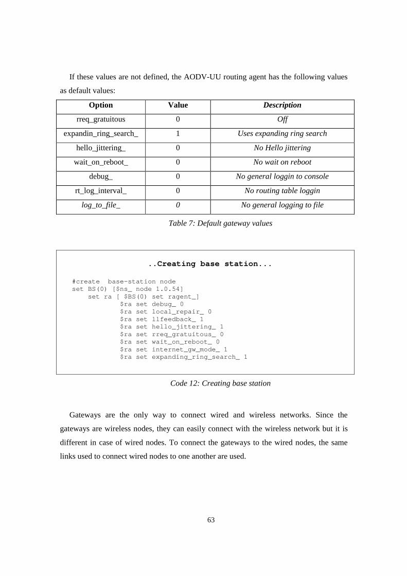
63
If these values are not defined, the AODV-UU routing agent has the following values
as default values:
Option Value Description
rreq_gratuitous 0 Off
expandin_ring_search_ 1 Uses expanding ring search
hello_jittering_ 0 No Hello jittering
wait_on_reboot_ 0 No wait on reboot
debug_ 0 No general loggin to console
rt_log_interval_ 0 No routing table loggin
log_to_file_ 0 No general logging to file
Table 7: Default gateway values
..Creating base station...
#create base-station node set BS(0) [$ns_ node 1.0.54] set ra [ $BS(0) set ragent_] $ra set debug_ 0 $ra set local_repair_ 0 $ra set llfeedback_ 1 $ra set hello_jittering_ 1 $ra set rreq_gratuitous_ 0 $ra set wait_on_reboot_ 0 $ra set internet_gw_mode_ 1 $ra set expanding_ring_search_ 1
Code 12: Creating base station
Gateways are the only way to connect wired and wireless networks. Since the
gateways are wireless nodes, they can easily connect with the wireless network but it is
different in case of wired nodes. To connect the gateways to the wired nodes, the same
links used to connect wired nodes to one another are used.
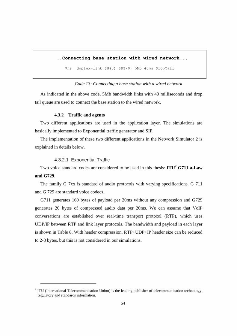
64
..Connecting base station with wired network...
$ns_ duplex-link $W(0) $BS(0) 5Mb 40ms DropTail
Code 13: Connecting a base station with a wired network
As indicated in the above code, 5Mb bandwidth links with 40 milliseconds and drop
tail queue are used to connect the base station to the wired network.
4.3.2 Traffic and agents
Two different applications are used in the application layer. The simulations are
basically implemented to Exponential traffic generator and SIP.
The implementation of these two different applications in the Network Simulator 2 is
explained in details below.
4.3.2.1 Exponential Traffic
Two voice standard codes are considered to be used in this thesis: ITU 2 G711 a-Law
and G729.
The family G 7xx is standard of audio protocols with varying specifications. G 711
and G 729 are standard voice codecs.
G711 generates 160 bytes of payload per 20ms without any compression and G729
generates 20 bytes of compressed audio data per 20ms. We can assume that VoIP
conversations are established over real-time transport protocol (RTP), which uses
UDP/IP between RTP and link layer protocols. The bandwidth and payload in each layer
is shown in Table 8. With header compression, RTP+UDP+IP header size can be reduced
to 2-3 bytes, but this is not considered in our simulations.
2 ITU (International Telecommunication Union) is the leading publisher of telecommunication technology,
regulatory and standards information.

65
Voice Codec G711 G729
Bandwidth (media layer) 64Kbps 8Kbps
Packet inter-arrival time 20ms 20ms
Voice packet length 160bytes 20bytes
RTP layer overhead 12bytes 12bytes
RTP layer packet size 172 bytes 32 bytes
RTP layer bandwidth 68,8 kbps 12,8 kbps
UDP layer overhead 8bytes 8bytes
UDP layer packet size 180 bytes 40 bytes
UDP layer bandwidth 72 kbps 16 kbps
IPv4 layer overhead 20 bytes 20 bytes
IPv4 packet size 200 bytes 60 bytes
IPv4 layer bandwidth 80 kbps 24 kbps
MAC layer overhead 36bytes 36bytes
PHY layer overhead 24bytes 24bytes
Table 8: G711 and G729 standard specifications
G729 is the chosen standard for our simulations. For simulation purposes we are
modelling a bi-directional VoIP conversation as a Markov process with idle and burst
time representing the voice activity in the conversation according to [28].
As stated, assuming each voice source as an on-off Markov process, the alternating
active (’on’) and silence (’off’) periods are exponentially distributed with average
durations of 350ms (‘on’) and 650ms (‘off’). Therefore, we consider an average talk spurt
of 35.0% and average silence period of 65.0% as recommended by the ITU-T3
3 The ITU Telecommunication Standarization Sector (ITU-T) coordinates standards for
telecommunications on behalf of the ITU(International Telecommunication Union)
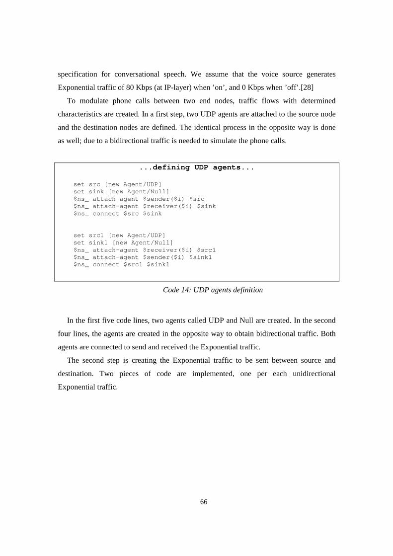
66
specification for conversational speech. We assume that the voice source generates
Exponential traffic of 80 Kbps (at IP-layer) when ’on’, and 0 Kbps when ’off’.[28]
To modulate phone calls between two end nodes, traffic flows with determined
characteristics are created. In a first step, two UDP agents are attached to the source node
and the destination nodes are defined. The identical process in the opposite way is done
as well; due to a bidirectional traffic is needed to simulate the phone calls.
...defining UDP agents...
set src [new Agent/UDP] set sink [new Agent/Null] $ns_ attach-agent $sender($i) $src $ns_ attach-agent $receiver($i) $sink $ns_ connect $src $sink set src1 [new Agent/UDP] set sink1 [new Agent/Null] $ns_ attach-agent $receiver($i) $src1 $ns_ attach-agent $sender($i) $sink1 $ns_ connect $src1 $sink1
Code 14: UDP agents definition
In the first five code lines, two agents called UDP and Null are created. In the second
four lines, the agents are created in the opposite way to obtain bidirectional traffic. Both
agents are connected to send and received the Exponential traffic.
The second step is creating the Exponential traffic to be sent between source and
destination. Two pieces of code are implemented, one per each unidirectional
Exponential traffic.
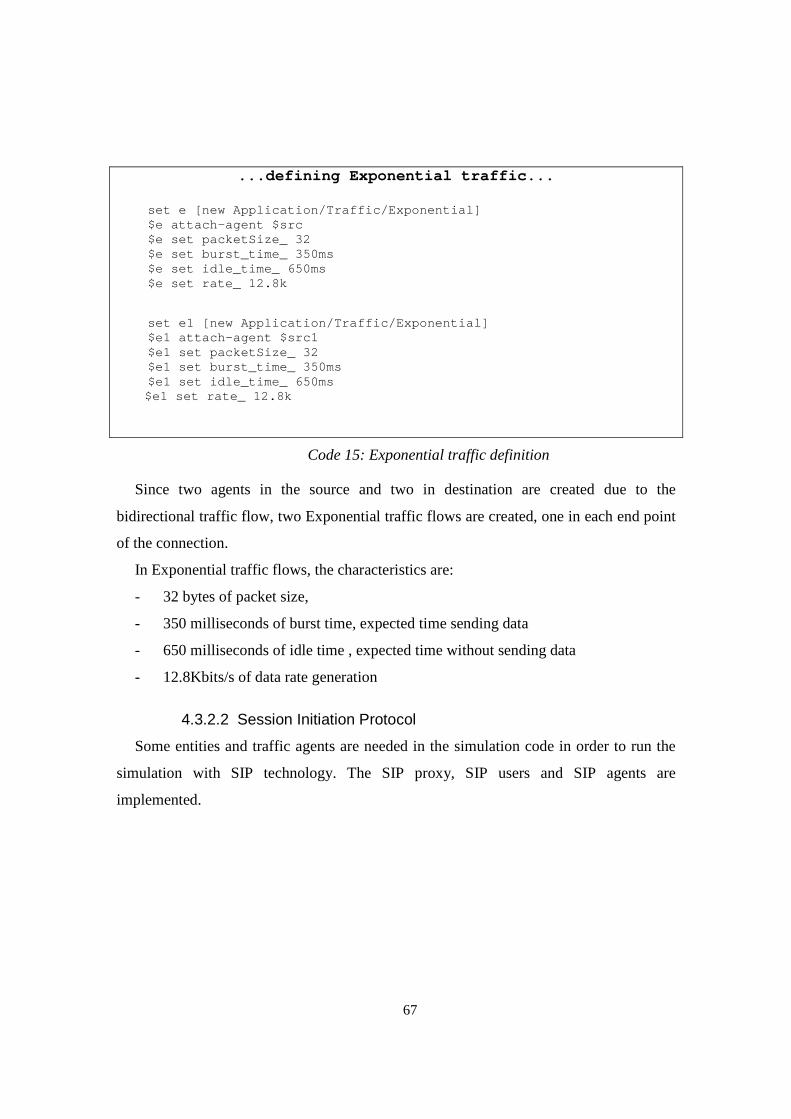
67
...defining Exponential traffic...
set e [new Application/Traffic/Exponential] $e attach-agent $src $e set packetSize_ 32 $e set burst_time_ 350ms $e set idle_time_ 650ms $e set rate_ 12.8k
set e1 [new Application/Traffic/Exponential] $e1 attach-agent $src1 $e1 set packetSize_ 32 $e1 set burst_time_ 350ms $e1 set idle_time_ 650ms $e1 set rate_ 12.8k
Code 15: Exponential traffic definition
Since two agents in the source and two in destination are created due to the
bidirectional traffic flow, two Exponential traffic flows are created, one in each end point
of the connection.
In Exponential traffic flows, the characteristics are:
- 32 bytes of packet size,
- 350 milliseconds of burst time, expected time sending data
- 650 milliseconds of idle time , expected time without sending data
- 12.8Kbits/s of data rate generation
4.3.2.2 Session Initiation Protocol
Some entities and traffic agents are needed in the simulation code in order to run the
simulation with SIP technology. The SIP proxy, SIP users and SIP agents are
implemented.
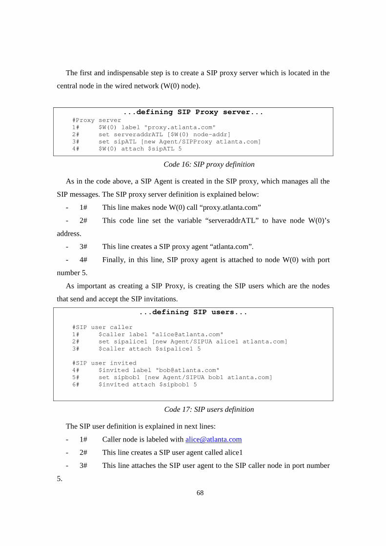
68
The first and indispensable step is to create a SIP proxy server which is located in the
central node in the wired network (W(0) node).
...defining SIP Proxy server... #Proxy server 1# $W(0) label "proxy.atlanta.com" 2# set serveraddrATL [$W(0) node-addr] 3# set sipATL [new Agent/SIPProxy atlanta.c om] 4# $W(0) attach $sipATL 5
Code 16: SIP proxy definition
As in the code above, a SIP Agent is created in the SIP proxy, which manages all the
SIP messages. The SIP proxy server definition is explained below:
- 1# This line makes node W(0) call “proxy.atlanta.com”
- 2# This code line set the variable “serveraddrATL” to have node W(0)’s
address.
- 3# This line creates a SIP proxy agent “atlanta.com”.
- 4# Finally, in this line, SIP proxy agent is attached to node W(0) with port
number 5.
As important as creating a SIP Proxy, is creating the SIP users which are the nodes
that send and accept the SIP invitations.
...defining SIP users... #SIP user caller 1# $caller label "[email protected]" 2# set sipalice1 [new Agent/SIPUA alice1 at lanta.com] 3# $caller attach $sipalice1 5 #SIP user invited 4# $invited label "[email protected]" 5# set sipbob1 [new Agent/SIPUA bob1 atlant a.com] 6# $invited attach $sipbob1 5
Code 17: SIP users definition
The SIP user definition is explained in next lines:
- 1# Caller node is labeled with [email protected]
- 2# This line creates a SIP user agent called alice1
- 3# This line attaches the SIP user agent to the SIP caller node in port number
5.

69
- 4# Caller node is labeled with [email protected].
- 5# This line creates a SIP user agent called bob1.
- 6# This line attaches the SIP user agent to the SIP caller node in port number
5.
The only step remaining is to initiate the components to make an invitation call. This
is done by setting the SIP proxy for each SIP user.
...setting SIP users to the proxy... #set SIP users in the SIP proxy $sipalice1 set-proxy $serveraddrATL
Code 18: set SIP user to the proxy
The two lines in Code 18 set the proxy to the SIP nodes. This is done by setting the
SIP proxy address to the SIP user agent.
The SIP user agent “sipalice1” is set to the SIP proxy address “serveraddrATL”.
4.3.3 Events schedule
After defining all the needed elements to run the simulations, the next step is to define
the events schedule, for example, which kind of events are chosen to run and when.
For Exponential traffic flows an example is given in Code 19.
...Schedule events for the Exponential agents... $ns_ at 5.0 "$e start" $ns_ at 5.0 "$e1 start" $ns_ at 185 "$e stop" $ns_ at 185 "$e1 stop"
Code 19: Schedule for Exponential traffic
As was defined earlier, the Exponential agents are “e” and “e1”. In the four lines in
Code 19, at second 5 the Exponential traffic is started and stopped at second 185.
For SIP events to use this protocol, the event schedule is a little bit more complex due
to the actions needed for having the invitation event. Figure 8 shows the action needed by

70
a SIP user in order to make an invitation call. As shown in Figure 8, SIP users have to
register, and then the SIP caller user sends an invitation request. And finally, to end the
call, both SIP users involved in the event send a bye request.
Figure 8: SIP invitation event tasks
The first step is that the SIP users register in the SIP proxy, see Code 20.
...SIP users registering in the proxy... $ns_ at 1 "$sipbob1 register" $ns_ at 1 "$sipalice1 register"
Code 20: Register SIP users
At second 1, the users “sipbob1” and ”sipalice1” register in the proxy server. When
they are both registered, any of them can start a SIP invitation, see Code 21.
...SIP user sends an invitation... $ns_ at 20 "$sipalice1 invite bob1 atlanta.com bw 32kb 64kb"
Code 21: SIP user sends an invitation
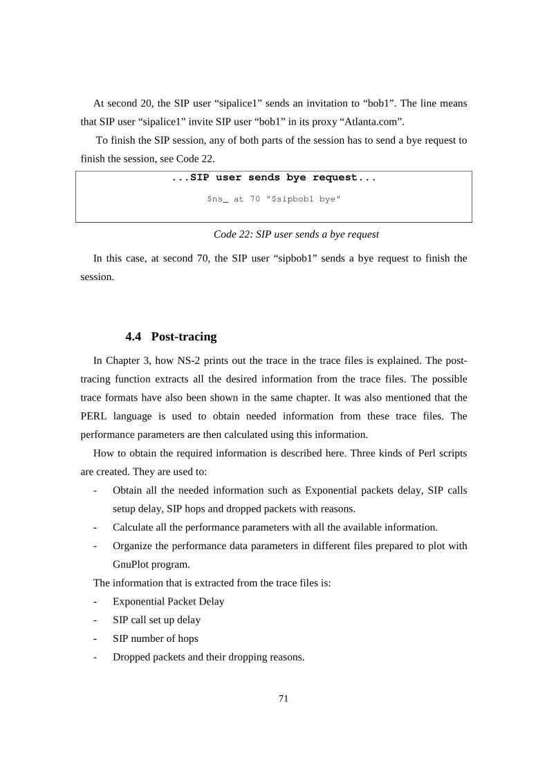
71
At second 20, the SIP user “sipalice1” sends an invitation to “bob1”. The line means
that SIP user “sipalice1” invite SIP user “bob1” in its proxy “Atlanta.com”.
To finish the SIP session, any of both parts of the session has to send a bye request to
finish the session, see Code 22.
...SIP user sends bye request...
$ns_ at 70 "$sipbob1 bye"
Code 22: SIP user sends a bye request
In this case, at second 70, the SIP user “sipbob1” sends a bye request to finish the
session.
4.4 Post-tracing
In Chapter 3, how NS-2 prints out the trace in the trace files is explained. The post-
tracing function extracts all the desired information from the trace files. The possible
trace formats have also been shown in the same chapter. It was also mentioned that the
PERL language is used to obtain needed information from these trace files. The
performance parameters are then calculated using this information.
How to obtain the required information is described here. Three kinds of Perl scripts
are created. They are used to:
- Obtain all the needed information such as Exponential packets delay, SIP calls
setup delay, SIP hops and dropped packets with reasons.
- Calculate all the performance parameters with all the available information.
- Organize the performance data parameters in different files prepared to plot with
GnuPlot program.
The information that is extracted from the trace files is:
- Exponential Packet Delay
- SIP call set up delay
- SIP number of hops
- Dropped packets and their dropping reasons.
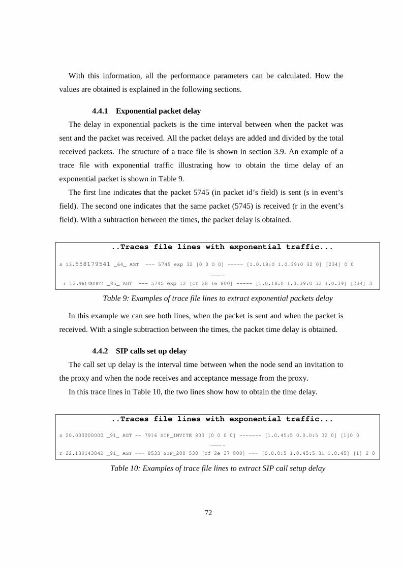
72
With this information, all the performance parameters can be calculated. How the
values are obtained is explained in the following sections.
4.4.1 Exponential packet delay
The delay in exponential packets is the time interval between when the packet was
sent and the packet was received. All the packet delays are added and divided by the total
received packets. The structure of a trace file is shown in section 3.9. An example of a
trace file with exponential traffic illustrating how to obtain the time delay of an
exponential packet is shown in Table 9.
The first line indicates that the packet 5745 (in packet id’s field) is sent (s in event’s
field). The second one indicates that the same packet (5745) is received (r in the event’s
field). With a subtraction between the times, the packet delay is obtained.
..Traces file lines with exponential traffic...
s 13. 558179541 _64_ AGT --- 5745 exp 32 [0 0 0 0] ----- [1.0.18: 0 1.0.39:0 32 0] [234] 0 0
………….
r 13. 961480874 _85_ AGT --- 5745 exp 12 [cf 28 1e 800] ----- [1. 0.18:0 1.0.39:0 32 1.0.39] [234] 3
Table 9: Examples of trace file lines to extract exponential packets delay
In this example we can see both lines, when the packet is sent and when the packet is
received. With a single subtraction between the times, the packet time delay is obtained.
4.4.2 SIP calls set up delay
The call set up delay is the interval time between when the node send an invitation to
the proxy and when the node receives and acceptance message from the proxy.
In this trace lines in Table 10, the two lines show how to obtain the time delay.
..Traces file lines with exponential traffic...
s 20.000000000 _91_ AGT -- 7916 SIP_INVITE 800 [0 0 0 0] ------- [1.0.45:5 0.0.0:5 32 0] [1]0 0
………….
r 22.139143842 _91_ AGT --- 8533 SIP_200 530 [cf 2e 37 800] --- [0.0.0:5 1.0.45:5 31 1.0.45] [1] 2 0
Table 10: Examples of trace file lines to extract SIP call setup delay
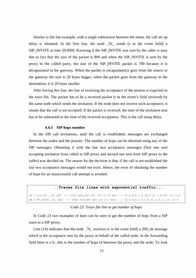
73
Similar to the last example; with a single subtraction between the times, the call set up
delay is obtained. In the first line, the node _91_ sends (s in the event field) a
SIP_INVITE at time 20.0000. Knowing if the SIP_INVITE was sent by the caller is easy
due to fact that the size of the packet is 800 and when the SIP_INVITE is sent by the
proxy to the called party, the size of the SIP_INVITE packet is 780 because it is
decapsulated in the gateway. When the packet is encapsulated,it goes from the source to
the gateway the size is 20 bytes bigger, when the packet goes from the gateway to the
destination, it is 20 bytes smaller.
After having this line, the line of receiving the acceptance of the session is expected in
the trace file. The packet has to be a received packet (r in the event’s field received) by
the same node which sends the invitation. If the node does not receive such acceptance, it
means that the call is not accepted. If the packet is received, the time of the invitation sent
has to be subtracted to the time of the received acceptance. This is the call setup delay.
4.4.3 SIP hops number
In the SIP call invitations, until the call is established, messages are exchanged
between the nodes and the proxies. The number of hops can be obtained using any of the
SIP messages. Obtaining it with the last two acceptance messages (first one sent
accepting invitation from called to SIP proxy and second one sent from SIP proxy to the
caller) was decided on. The reason for the decision is that, if the call is not established the
last two acceptance messages would not exist. Hence, the error of obtaining the number
of hops for an unsuccessful call attempt is avoided.
..Traces file lines with exponential traffic...
1# r 118.367 _76_ AGT --- 3101 SIP_200 530 [cf 1f 20 80] --- [0.0.0:5 1.0.30:5 31 1.0.30] [1] 6 0
2# r 99.28497 _47_ AGT --- 2680 SIP_ACK 280 [cf 2 c 800] --- [0.0.0:5 1.0.1:5 31 1.0.1] [1] 10 0
Code 23: Trace file line to get number of hops
In Code 23 two examples of lines can be seen to get the number of hops from a SIP
users to a SIP proxy.
Line (1#) indicates that the node _76_ receives (r in the event field) a 200_ok message
which is the acceptance sent by the proxy in behalf of the called node. In the forwarding
field there is a 6 , this is the number of hops of between the proxy and the node. To look
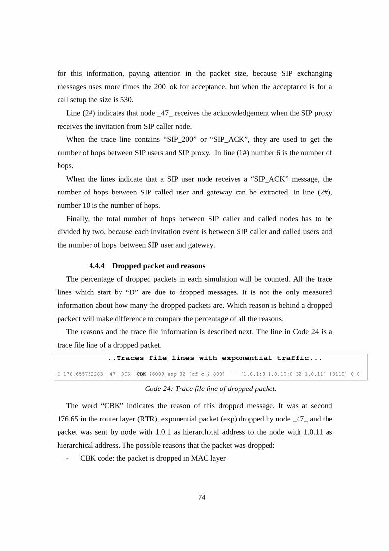
74
for this information, paying attention in the packet size, because SIP exchanging
messages uses more times the 200_ok for acceptance, but when the acceptance is for a
call setup the size is 530.
Line (2#) indicates that node _47_ receives the acknowledgement when the SIP proxy
receives the invitation from SIP caller node.
When the trace line contains “SIP_200” or “SIP_ACK”, they are used to get the
number of hops between SIP users and SIP proxy. In line (1#) number 6 is the number of
hops.
When the lines indicate that a SIP user node receives a “SIP_ACK” message, the
number of hops between SIP called user and gateway can be extracted. In line (2#),
number 10 is the number of hops.
Finally, the total number of hops between SIP caller and called nodes has to be
divided by two, because each invitation event is between SIP caller and called users and
the number of hops between SIP user and gateway.
4.4.4 Dropped packet and reasons
The percentage of dropped packets in each simulation will be counted. All the trace
lines which start by “D” are due to dropped messages. It is not the only measured
information about how many the dropped packets are. Which reason is behind a dropped
packect will make difference to compare the percentage of all the reasons.
The reasons and the trace file information is described next. The line in Code 24 is a
trace file line of a dropped packet.
..Traces file lines with exponential traffic...
D 176.655752283 _47_ RTR CBK 46009 exp 32 [cf c 2 800] --- [1.0.1:0 1.0.10:0 32 1.0.11] [3110] 0 0
Code 24: Trace file line of dropped packet.
The word “CBK” indicates the reason of this dropped message. It was at second
176.65 in the router layer (RTR), exponential packet (exp) dropped by node _47_ and the
packet was sent by node with 1.0.1 as hierarchical address to the node with 1.0.11 as
hierarchical address. The possible reasons that the packet was dropped:
- CBK code: the packet is dropped in MAC layer
75
- IFQ code: indicates that the packet is dropped because there is not enough space
in the buffer queue.
- ARP code: indicates that the packet is dropped in ARP (address resolution
protocol).
- NRTE code: indicates that the packet is dropped in routing layer due to not
available route.
- LOOP code: packet dropped in routing layer due to routing loop.
- TOUT code: packet dropped in routing layer due to time packet expired.
All these reasons will be grouped in three groups due to the reason character.
1st group: Dropped packets due to MAC layer (CBK code)
2nd group: Dropped packets due to congestion in the queue (IFQ and ARP codes).
3rd group: Dropped packets due to routing layer reasons (NRTE, LOOP, TTL,
TOUT codes)
4.5 Performance Parameters and scalability
To understand the simulation results that we obtain is important. Varying the number
of gateways, the number of hops and the number of voice traffic flows, there many
different simulations.
The basic scenarios are 1 gateway scenario, 2 gateway scenario and 4 gateway
scenario. Each scenario has 6 different numbers of hops between sources and destinations
in simulations (2 hops, 3 hops, 4 hops, 5 hops, 6 hops and 7 hops).
And each one has 6 different number of background traffic flows (4 flows, 8 flows, 12
flows, 16 flows, 24 flows, 32 flows). Therefore the simulations are already 108 (3 x 6 x
6), and each simulation will be repeated 5 times with different SIP call participants.
All these simulations generate a lot of information. However, this is too much
information to evaluate manually how the network performance in the different situations
is.
Some important parameters (performance parameters) are defined to see the most
important and relevant information about the network behavior. The parameters
calculated are discussed in the following sections:
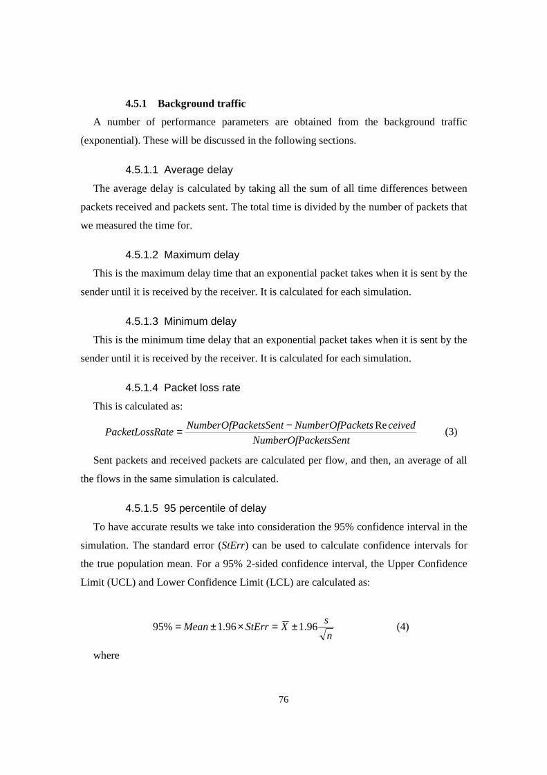
76
4.5.1 Background traffic
A number of performance parameters are obtained from the background traffic
(exponential). These will be discussed in the following sections.
4.5.1.1 Average delay
The average delay is calculated by taking all the sum of all time differences between
packets received and packets sent. The total time is divided by the number of packets that
we measured the time for.
4.5.1.2 Maximum delay
This is the maximum delay time that an exponential packet takes when it is sent by the
sender until it is received by the receiver. It is calculated for each simulation.
4.5.1.3 Minimum delay
This is the minimum time delay that an exponential packet takes when it is sent by the
sender until it is received by the receiver. It is calculated for each simulation.
4.5.1.4 Packet loss rate
This is calculated as:
cketsSentNumberOfPa
ceivedcketsNumberOfPacketsSentNumberOfPaRatePacketLoss
Re−= (3)
Sent packets and received packets are calculated per flow, and then, an average of all
the flows in the same simulation is calculated.
4.5.1.5 95 percentile of delay
To have accurate results we take into consideration the 95% confidence interval in the
simulation. The standard error (StErr) can be used to calculate confidence intervals for
the true population mean. For a 95% 2-sided confidence interval, the Upper Confidence
Limit (UCL) and Lower Confidence Limit (LCL) are calculated as:
n
sXStErrMean 96.196.1%95 ±=×±= (4)
where

77
n
s
n
DeviationdardSStErr == _tan
(5)
is the standard error and
∑=
−=N
ii XX
Ns
1
2)(1
(6)
is the standard deviation.
Where Standard Deviation (s) can be calculated as:
The standard seviation (s) of a discrete uniform random variable X can be calculated
as follows:
1 - For each value Xi, calculate the difference XX i − between Xi and the average
value X
2 - Calculate the squares of these differences.
3 - Find the average of the squared differences. This quantity is the variance
4 - Take the square root of the variance.
At the end you have the standard deviation (s) that can be applied to the equation 5 to
obtain the 95% confidence interval (UCL and LCL).
4.5.2 SIP invitation calls
In this section, the performance parameters obtained from SIP flows are explained.
4.5.2.1 Call set up Delay Average
The call set up delay is the time elapsed since the SIP caller node sends an invitation
until the same node receives the acceptance message. The average is calculated with all
the call setup times of the same simulation. For example, one simulation setup is 1
gateway, 2 hops, 4 flows, 5 repetitions in which there are 100 call invitations in total.
4.5.2.2 Minimum set up delay
This is the minimum value of all call setup delays taken from all SIP call invitations of
each simulation.
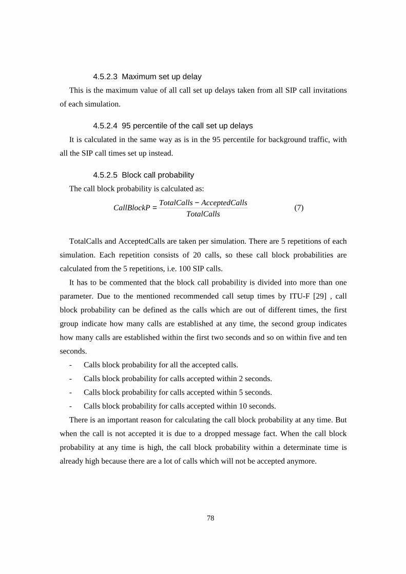
78
4.5.2.3 Maximum set up delay
This is the maximum value of all call set up delays taken from all SIP call invitations
of each simulation.
4.5.2.4 95 percentile of the call set up delays
It is calculated in the same way as is in the 95 percentile for background traffic, with
all the SIP call times set up instead.
4.5.2.5 Block call probability
The call block probability is calculated as:
TotalCalls
llsAcceptedCaTotalCallsCallBlockP
−= (7)
TotalCalls and AcceptedCalls are taken per simulation. There are 5 repetitions of each
simulation. Each repetition consists of 20 calls, so these call block probabilities are
calculated from the 5 repetitions, i.e. 100 SIP calls.
It has to be commented that the block call probability is divided into more than one
parameter. Due to the mentioned recommended call setup times by ITU-F [29] , call
block probability can be defined as the calls which are out of different times, the first
group indicate how many calls are established at any time, the second group indicates
how many calls are established within the first two seconds and so on within five and ten
seconds.
- Calls block probability for all the accepted calls.
- Calls block probability for calls accepted within 2 seconds.
- Calls block probability for calls accepted within 5 seconds.
- Calls block probability for calls accepted within 10 seconds.
There is an important reason for calculating the call block probability at any time. But
when the call is not accepted it is due to a dropped message fact. When the call block
probability at any time is high, the call block probability within a determinate time is
already high because there are a lot of calls which will not be accepted anymore.

79
4.5.2.6 Number of hops average
This is the average of the number of hops in the 100 SIP calls in the 5 repetitions of
one simulation. All SIP calls are between two nodes inside the MANET, but the SIP
invitation messages go to a SIP proxy outside the MANET through the gateways. The
number of hops is calculated in the last invitation message, which is the acceptance
message (SIP 200 OK), and the number of hops are the number of hops which this
message goes from the called party to the gateway and number of hops between the
gateway and the caller party.
4.5.2.7 Calls per time
One graph per each simulation will be created with the times when the sip calls are
accepted. That means, the graphic will contain two parameters. The first show how many
calls are accepted in each second, and the second parameter shows how many calls are
accepted until each second.
4.5.2.8 SIP invitation attempts
SIP invitation attempts mean how many invitation messages the caller nodes send.
There are two reasons of why one node sends more than one invitation message. The first
is that the SIP caller user does not get the “100 trying” message. When the caller node
sends the first invitation message, it waits 0.5 seconds for the “100 trying” message
which comes from the SIP proxy. If “100 trying” message does not arrive, the node will
resend the invitation, the second time, it will wait the same time plus the double of the
time, so 1.5 seconds and so on.
The second reason is because of dropped messages. If the invitation message or the
“100 trying” message is dropped, the SIP caller user node will resend the invitation
message as it does when the first reason happens.
The calculation of this performance parameter will be divided in two steps. In the first
step the number of invitation messages in total the SIP caller users send is calculated and
in the second step the number of resent invitation messages is calculated because of
dropped messages and because of the delay reason.
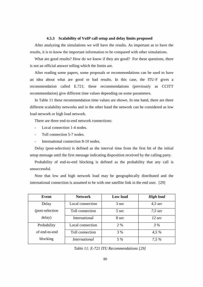
80
4.5.3 Scalability of VoIP call setup and delay limits proposed
After analyzing the simulations we will have the results. As important as to have the
results, it is to know the important information to be compared with other simulations.
What are good results? How do we know if they are good? For these questions, there
is not an official answer telling which the limits are.
After reading some papers, some proposals or recommendations can be used to have
an idea about what are good or bad results. In this case, the ITU-F gives a
recommendation called E.721; these recommendations (previously as CCITT
recommendation) give different time values depending on some parameters.
In Table 11 these recommendation time values are shown. In one hand, there are three
different scalability networks and in the other hand the network can be considered as low
load network or high load network.
There are three end-to-end network connections:
- Local connection 1-4 nodes.
- Toll connection 5-7 nodes.
- International connection 8-10 nodes.
Delay (post-selection) is defined as the interval time from the first bit of the initial
setup message until the first message indicating disposition received by the calling party.
Probability of end-to-end blocking is defined as the probability that any call is
unsuccessful.
Note that low and high network load may be geographically distributed and the
international connection is assumed to be with one satellite link in the end user. [29]
Event Network Low load High load
Local connection 3 sec 4,5 sec
Toll connection 5 sec 7,5 sec
Delay
(post-selection
delay) International 8 sec 12 sec
Local connection 2 % 3 %
Toll connection 3 % 4,5 %
Probability
of end-to-end
blocking International 5 % 7,5 %
Table 11: E-721 ITU Recommendations [29]

81

82
5 Evaluation of simulations
In this chapter, we describe details of several simulation scenarios and the obtained
results how are calculated from the simulations as well.
The first part describes the simulation scenarios that have been used. The second part
describes the several different traffic scenarios created during the simulations.
The third part presents the performance results obtained througth post processing
analysis of simulation results. It describes the evaluation of session call establishement
and voice quality analysis.
5.1 Simulation Scenarios
All the simulations were run using static scenarios. Every scenario is composed by one
hundred mobile nodes and forty two wired nodes. The mobile nodes are static and are
arranged in the following structure:
- The nodes form a grid of 10 x 10 and are separated by 200 meters. Thus the grid
is 2000 meters by 2000 meters.
- Although, the one hundred mobile nodes are always in the same place, three
different simulation scenarios were created depending on how many mobile nodes
are acting as gateway. One, two and four are the number of mobile nodes which
can act as gateways. This is illustrated in Figure 10 a, b and c respectively.
83
Figure 9:Basic Scenario
In Figure 9, the green circles are the wireless nodes and the blue ones are the wired
nodes. All the lines are the wired connections between wired nodes (as showed in the last
chapter, 5 Mb wired connections with 40 milliseconds delay).
Figure 10 shows the three different scenarios depending on the number of wireless
nodes acting as gateways which are depicted in red dots. Figure a, b and c depicts one,
two and four gateways scenarios.
(a)
(b)
(c)
Figure 10: Scenarios with 1 (a), 2 (b) and 4 (c) gateways

84
5.2 Traffic Scenario
As stated earlier, in the application layer there are two types of events in the
simulations. On one hand, different traffic flows modeling phone calls are running in a
full time during all the simulations and these are called background traffic calls. On the
other hand, a determinate number of SIP users try to establish SIP sessions at different
times. Both cases are explained further below.
5.2.1 Background Traffic Scenario
In this scenario, background traffic is running during the simulations. Why is called
background traffic? In these simulations, SIP invitation calls are the most important
aspect. However in every simulation there are some exponential traffic flows modeling
phone calls (VoIP traffic) called background traffic because it is running in background
during the whole simulation.
For each simulation there are different numbers of background traffic flows
representing different network load; these background traffic flows are differentiated
depending on the number of hops between source and destination. The simulations are
classified depending on the number of traffic flows. The traffic flows are always divided
in two groups (75% of them are inside the MANET and 25% of them goes to outside the
MANET) .They are called inside and outgoing traffic flows respectively. There are six
different number of traffic flows:
- Four background traffic flows:
� Three between wireless nodes
� One between one wireless node and one wired one.
- Eight background traffic flows:
� Six between wireless nodes
� Two between wireless nodes and wired nodes
- Twelve background traffic flows:
� Nine between wireless nodes
� Three between wireless nodes and wired nodes.
- Sixteen background traffic flows:
� Twelve between wireless nodes
� Four between wireless nodes and wired nodes
85
- Twenty four background traffic flows:
� Eighteen between wireless nodes
� Six between wireless nodes and wired nodes
- Thirty two background traffic flows:
� Twenty four between wireless nodes
� Six between wireless nodes and wired nodes
Note that all nodes are chosen randomly; the source and destination nodes for all
exponential traffic flows are attached in the appendix in section B.1.4. One of the aims of
our approach is that 25% of the exponential traffic flows are between nodes inside the
network and nodes outside the network, and the 75% of exponential traffic flows are
inside the network.
As defined in our approach, each simulation is repeated for the following values of
number of hops in the background traffic:
2 hops, 3 hops, 4 hops, 5 hops, 6hops and 7 hops.
The number of hops is between the source node and destination node when the traffic
is inside the Ad Hoc Network. However it is between the source node and the gateway
when the traffic is between a wireless node and a wired node.
Note that the source and destination nodes in the simulation scenarios are defined with
one gateway in terms of number of hops. And afterwards, two and four gateways
simulations are added maintaining the same source and destinations background traffic
flows. Therefore the number of hops between the source and the gateways can be
different when there are more gateways.
5.2.2 SIP calls traffic scenario
The SIP call traffic scenario is the most important part of the simulations. Since the
goal of the dissertation is to determine the behavior and the performance of VoIP in
hybrid MANETS in different traffic scenarios, the SIP calls scenario will be critical in
determining our results.
During the simulation we adopt the premise that a node can not participate in more
than one voice conversation.
In order to have a good average, it was decided that having 100 SIP invitation calls is
a good number to have accurate results in order to see and study SIP calls behavior. For
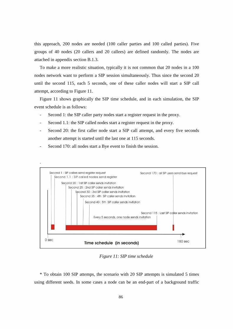
86
this approach, 200 nodes are needed (100 caller parties and 100 called parties). Five
groups of 40 nodes (20 callers and 20 callees) are defined randomly. The nodes are
attached in appendix section B.1.3.
To make a more realistic situation, typically it is not common that 20 nodes in a 100
nodes network want to perform a SIP session simultaneously. Thus since the second 20
until the second 115, each 5 seconds, one of these caller nodes will start a SIP call
attempt, according to Figure 11.
Figure 11 shows graphically the SIP time schedule, and in each simulation, the SIP
event schedule is as follows:
- Second 1: the SIP caller party nodes start a register request in the proxy.
- Second 1.1: the SIP called nodes start a register request in the proxy.
- Second 20: the first caller node start a SIP call attempt, and every five seconds
another attempt is started until the last one at 115 seconds.
- Second 170: all nodes start a Bye event to finish the session.
.
Figure 11: SIP time schedule
* To obtain 100 SIP attemps, the scenario with 20 SIP attempts is simulated 5 times
using different seeds. In some cases a node can be an end-part of a background traffic

87
flow and an end-part of a SIP call as well. It is not possible to avoid because, the network
have 100 nodes, which are already used for SIP events during the 5 repetitions. Therefore
many nodes will be overlap with background traffic and SIP call events.
5.3 Simulation Evaluation
Chapter 4 describes the design and implementation simulation scenarios. How to
extract the needed information from the trace files and calculate the performance
parameters is defined in 4.4 (Post-tracing) and 4.5 (Performance Parameters and
Scalability).
In next points, the evaluation of all this information is described and commented. To
evaluate the performance of voice calls in hybrid MANETs, two different aspects of
results can be located at separately. The first one (section 5.3.1) evaluates the
performance parameters of Session Call Establishment. The second one (section 5.3.2)
evaluates the performance parameters of Voice Quality and Voice Capacity in all the
possible scenarios (described in 5.1 and 5.2).
5.3.1 Evaluation of Session Call Establishment
All the relevant performance parameters related with session initiation are commented
in this part. They are all calculated from the trace files such as SIP call setup delay times,
number of hops in SIP established calls and number of SIP attempts per simulation.
5.3.1.1 Time Call Setup
The average of SIP accepted call setup delays depending on the number of flows and
on the number of gateways in each simulation scenario are shown in the next graphs. The
most important thing is to check what the call setup delays are depending on the number
of gateways involved in the scenario.
Figure 12 and Figure 13 show the call setup delay for 2 hops and 7 hops respectively;
in each case the values when having 1, 2 and 4 gateways in the scenario are compared.
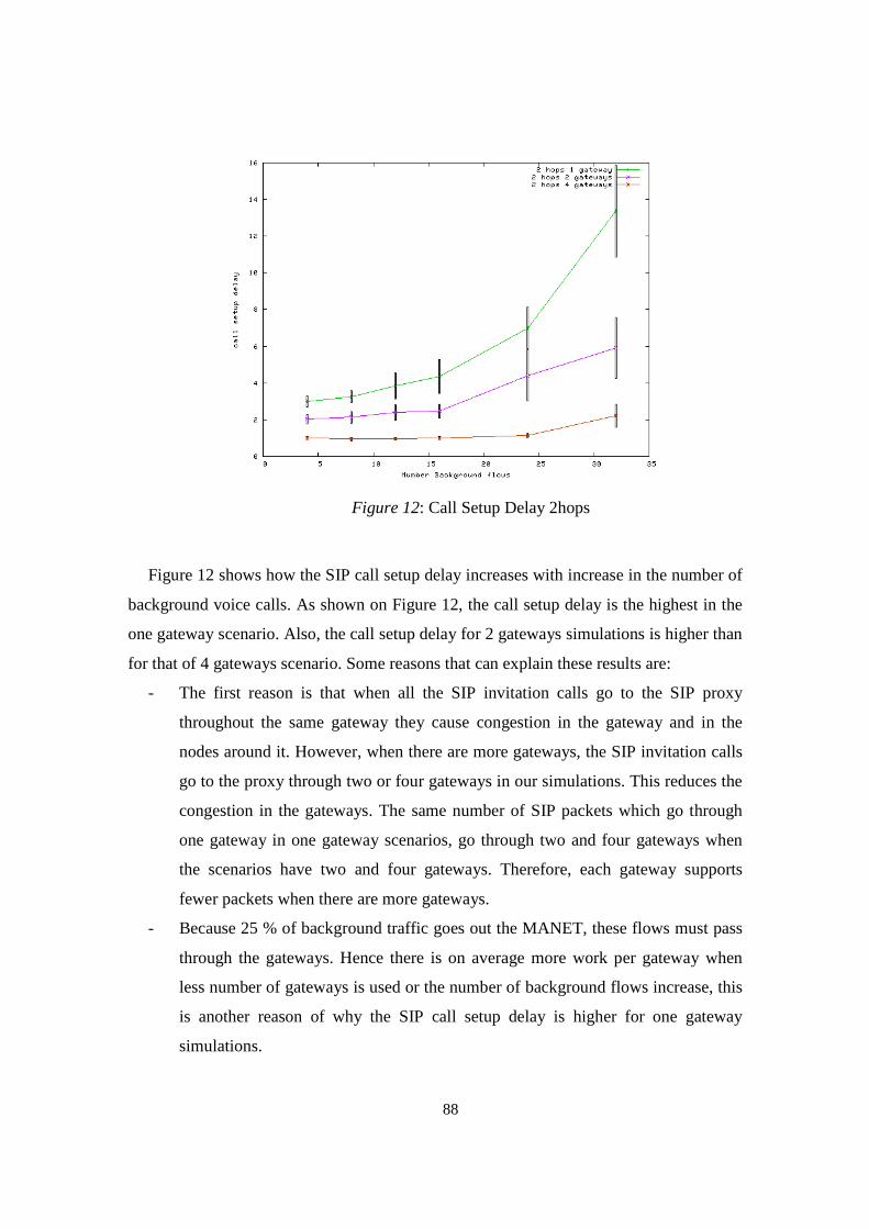
88
Figure 12: Call Setup Delay 2hops
Figure 12 shows how the SIP call setup delay increases with increase in the number of
background voice calls. As shown on Figure 12, the call setup delay is the highest in the
one gateway scenario. Also, the call setup delay for 2 gateways simulations is higher than
for that of 4 gateways scenario. Some reasons that can explain these results are:
- The first reason is that when all the SIP invitation calls go to the SIP proxy
throughout the same gateway they cause congestion in the gateway and in the
nodes around it. However, when there are more gateways, the SIP invitation calls
go to the proxy through two or four gateways in our simulations. This reduces the
congestion in the gateways. The same number of SIP packets which go through
one gateway in one gateway scenarios, go through two and four gateways when
the scenarios have two and four gateways. Therefore, each gateway supports
fewer packets when there are more gateways.
- Because 25 % of background traffic goes out the MANET, these flows must pass
through the gateways. Hence there is on average more work per gateway when
less number of gateways is used or the number of background flows increase, this
is another reason of why the SIP call setup delay is higher for one gateway
simulations.
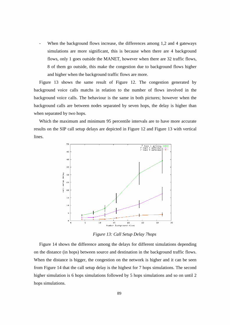
89
- When the background flows increase, the differences among 1,2 and 4 gateways
simulations are more significant, this is because when there are 4 background
flows, only 1 goes outside the MANET, however when there are 32 traffic flows,
8 of them go outside, this make the congestion due to background flows higher
and higher when the background traffic flows are more.
Figure 13 shows the same result of Figure 12. The congestion generated by
background voice calls matchs in relation to the number of flows involved in the
background voice calls. The behaviour is the same in both pictures; however when the
background calls are between nodes separated by seven hops, the delay is higher than
when separated by two hops.
Which the maximum and minimum 95 percentile intervals are to have more accurate
results on the SIP call setup delays are depicted in Figure 12 and Figure 13 with vertical
lines.
Figure 13: Call Setup Delay 7hops
Figure 14 shows the difference among the delays for different simulations depending
on the distance (in hops) between source and destination in the background traffic flows.
When the distance is bigger, the congestion on the network is higher and it can be seen
from Figure 14 that the call setup delay is the highest for 7 hops simulations. The second
higher simulation is 6 hops simulations followed by 5 hops simulations and so on until 2
hops simulations.

90
Figure 14: Call Setup Delay 1 gateway
Another point of view is seeing when the SIP calls are accepted in the different
simulation scenarios. Figure 15 and Figure 16 show when the SIP calls are established in
the scenario with 2 hops and 4 background flows simulation and in 5 hops and 24
background flows simulation respectively. These two graphs show the percentage of SIP
calls accepted every 100 milliseconds. The different times depending on the number of
gateways in each simulation is shown in each graph. Figure 15 shows the number of
accepted calls every 100 milliseconds in the simulation with 2 hops background voice
calls and 4 background voice calls. Theoretically this is the best case for the results,
because 2 hops and 4 background flows are the parameters that causes less congestion.
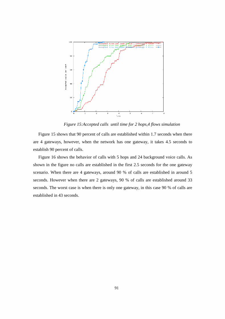
91
Figure 15:Accepted calls until time for 2 hops,4 flows simulation
Figure 15 shows that 90 percent of calls are established within 1.7 seconds when there
are 4 gateways, however, when the network has one gateway, it takes 4.5 seconds to
establish 90 percent of calls.
Figure 16 shows the behavior of calls with 5 hops and 24 background voice calls. As
shown in the figure no calls are established in the first 2.5 seconds for the one gateway
scenario. When there are 4 gateways, around 90 % of calls are established in around 5
seconds. However when there are 2 gateways, 90 % of calls are established around 33
seconds. The worst case is when there is only one gateway, in this case 90 % of calls are
established in 43 seconds.
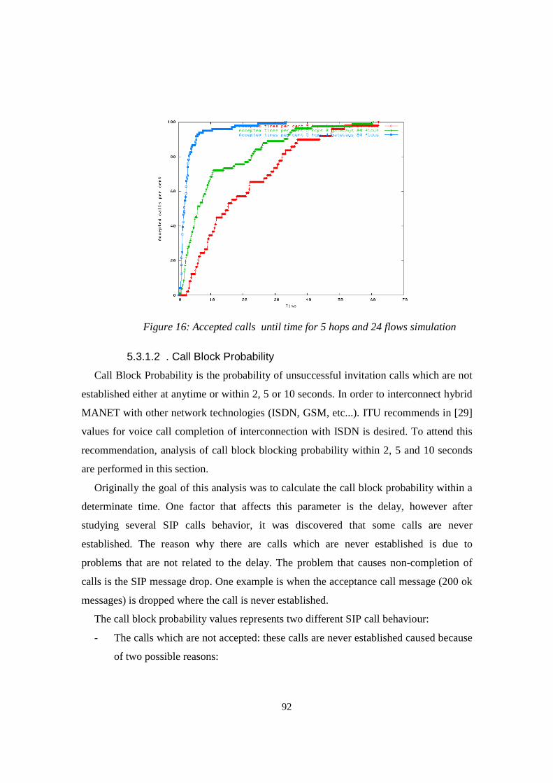
92
Figure 16: Accepted calls until time for 5 hops and 24 flows simulation
5.3.1.2 . Call Block Probability
Call Block Probability is the probability of unsuccessful invitation calls which are not
established either at anytime or within 2, 5 or 10 seconds. In order to interconnect hybrid
MANET with other network technologies (ISDN, GSM, etc...). ITU recommends in [29]
values for voice call completion of interconnection with ISDN is desired. To attend this
recommendation, analysis of call block blocking probability within 2, 5 and 10 seconds
are performed in this section.
Originally the goal of this analysis was to calculate the call block probability within a
determinate time. One factor that affects this parameter is the delay, however after
studying several SIP calls behavior, it was discovered that some calls are never
established. The reason why there are calls which are never established is due to
problems that are not related to the delay. The problem that causes non-completion of
calls is the SIP message drop. One example is when the acceptance call message (200 ok
messages) is dropped where the call is never established.
The call block probability values represents two different SIP call behaviour:
- The calls which are not accepted: these calls are never established caused because
of two possible reasons:

93
o Due to the delay of receiving the “100 trying” message, explained in
section 4.5.2.8), the caller node send re-invitations after the waiting time. If
another “100 trying” us bit received in 32 seconds, the session is expired
implying in no call completion.
o Due to a “200 ok” message is dropped. When the “200 ok” from the called
node to the proxy is dropped, there is no more chances to establish the call.
When the called node send an acceptance with “200 ok” message,it goes to
the busy state and any node can not try to invite him again,
- The calls which are not accepted within a concrete time: in this dissertation, three
different times are defined to calculate the call block probability (2, 5 and 10
seconds). This call block probability in this case, indicates the number of calls
which are not established within such times.
Table 12 contains the information of the call block probability at any time for all
simulations. In this table results, no restriction of time (2, 5 and 10 seconds) are applied,
and these results are used to calculate what is the amount of blocking probability which
are related to dropped message
Nº Gateways background 2 hops 3 hops 4 hops 5 hops 6 hops 7 hops 4 0.04 0.05 0.1 0.07 0.04 0.04 8 0.01 0.02 0.14 0.08 0.07 0.13 12 0.11 0.14 0.19 0.12 0.31 0.14 16 0.12 0.24 0.13 0.11 0.31 0.42 24 0.14 0.23 0.34 0.51 0.65 0.73
1
32 0.29 0.38 0.42 0.83 0.89 0.95 4 0.01 0.04 0.03 0.06 0.07 0.01 8 0.06 0.06 0.04 0.1 0.09 0.06 12 0.04 0.12 0.1 0.13 0.16 0.12 16 0.09 0.1 0.14 0.15 0.28 0.13 24 0.15 0.13 0.28 0.18 0.19 0.2
2
32 0.2 0.14 0.28 0.4 0.48 0.33 4 0.02 0.04 0 0.04 0.03 0.02 8 0.06 0.03 0.01 0.04 0.02 0.05 12 0.04 0.05 0.04 0.05 0 0.02 16 0.07 0.1 0.05 0.06 0.04 0.03 24 0.06 0.08 0.17 0.03 0.12 0.18
4
32 0.06 0.12 0.12 0.12 0.15 0.2
Table 12:Call block probability
In Figure 17, the call block probability for simulations with 7 hops is shown.
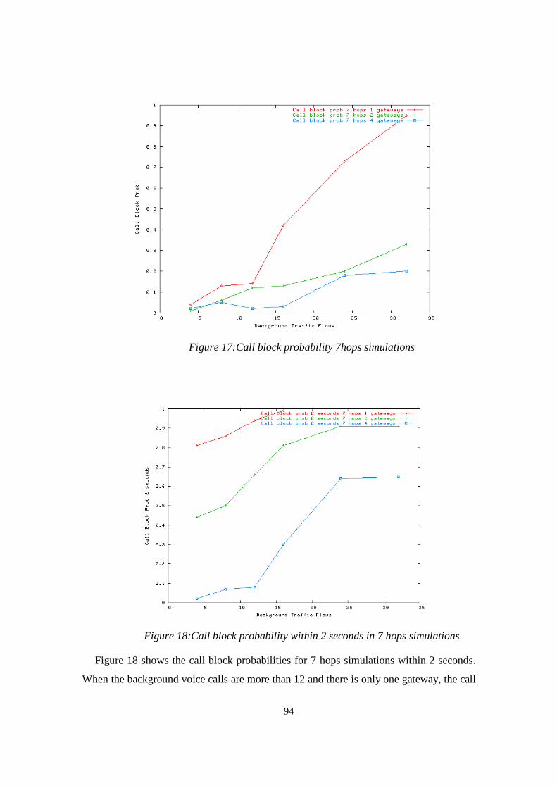
94
Figure 17:Call block probability 7hops simulations
Figure 18:Call block probability within 2 seconds in 7 hops simulations
Figure 18 shows the call block probabilities for 7 hops simulations within 2 seconds.
When the background voice calls are more than 12 and there is only one gateway, the call
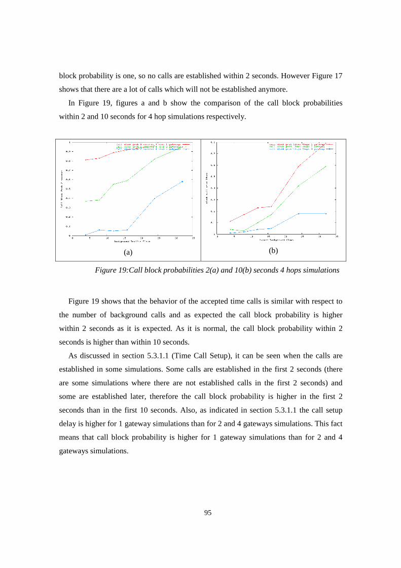
95
block probability is one, so no calls are established within 2 seconds. However Figure 17
shows that there are a lot of calls which will not be established anymore.
In Figure 19, figures a and b show the comparison of the call block probabilities
within 2 and 10 seconds for 4 hop simulations respectively.
(a)
(b)
Figure 19:Call block probabilities 2(a) and 10(b) seconds 4 hops simulations
Figure 19 shows that the behavior of the accepted time calls is similar with respect to
the number of background calls and as expected the call block probability is higher
within 2 seconds as it is expected. As it is normal, the call block probability within 2
seconds is higher than within 10 seconds.
As discussed in section 5.3.1.1 (Time Call Setup), it can be seen when the calls are
established in some simulations. Some calls are established in the first 2 seconds (there
are some simulations where there are not established calls in the first 2 seconds) and
some are established later, therefore the call block probability is higher in the first 2
seconds than in the first 10 seconds. Also, as indicated in section 5.3.1.1 the call setup
delay is higher for 1 gateway simulations than for 2 and 4 gateways simulations. This fact
means that call block probability is higher for 1 gateway simulations than for 2 and 4
gateways simulations.

96
5.3.1.3 Invitation Attempts
In chapter 2, how SIP works was shown. In section 5.2.2 (SIP calls traffic scenario)
SIP traffic schedule was defined. One hundred SIP caller users invite one hundred SIP
called users. These one hundred caller users send one hundred invitation messages to the
SIP proxy. If the SIP caller does not receive the “100 trying” confirmation message in a
determinate time (explained in section 4.5.2.8) which indicate that the invitation message
was received by the SIP proxy, the SIP caller resends the invitation. There may be
different reasons why SIP caller does not receive the “100 trying” message. It may be
because one of the message is dropped or because of the delay.
The Figure 20 shows the best and the worst case related with the number of SIP
invitation attempts.
(a)
(b)
Figure 20: Invitation attempts in 2(a) and 7(b) hops simulations
In Figure 20, the invitation attempts follow the same pattern in both, 2 and 7 hops
simulations (figures a and b respectively). There is increase in the invitation attempts
when the background voice calls increase. However, the number of invitation attempts is
much higher for 7 hops simulation scenarios. This number indicates how many times the
100 SIP caller nodes send invitations (including the first invitation).
In the next figures, Figure 21 and Figure 22, the number of invitation messages can be
seen with its respectively reasons, which are:
- the first 100 invitation attempts initiated by user agents (blue)
- the resent invitations due to dropping message reasons (yellow).
- the resent invitations due to timeout reasons (red).
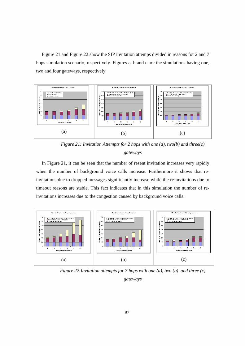
97
Figure 21 and Figure 22 show the SIP invitation attemps divided in reasons for 2 and 7
hops simulation scenario, respectively. Figures a, b and c are the simulations having one,
two and four gateways, respectively.
(a)
(b)
(c)
Figure 21: Invitation Attempts for 2 hops with one (a), two(b) and three(c)
gateways
In Figure 21, it can be seen that the number of resent invitation increases very rapidly
when the number of background voice calls increase. Furthermore it shows that re-
invitations due to dropped messages significantly increase while the re-invitations due to
timeout reasons are stable. This fact indicates that in this simulation the number of re-
invitations increases due to the congestion caused by background voice calls.
(a)
(b)
(c)
Figure 22:Invitation attempts for 7 hops with one (a), two (b) and three (c)
gateways
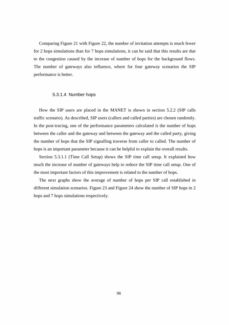
98
Comparing Figure 21 with Figure 22, the number of invitation attempts is much fewer
for 2 hops simulations than for 7 hops simulations, it can be said that this results are due
to the congestion caused by the increase of number of hops for the background flows.
The number of gateways also influence, where for four gateway scenarios the SIP
performance is better.
5.3.1.4 Number hops
How the SIP users are placed in the MANET is shown in section 5.2.2 (SIP calls
traffic scenario). As described, SIP users (callers and called parties) are chosen randomly.
In the post-tracing, one of the performance parameters calculated is the number of hops
between the caller and the gateway and between the gateway and the called party, giving
the number of hops that the SIP signalling traverse from caller to called. The number of
hops is an important parameter because it can be helpful to explain the overall results.
Section 5.3.1.1 (Time Call Setup) shows the SIP time call setup. It explained how
much the increase of number of gateways help to reduce the SIP time call setup. One of
the most important factors of this improvement is related to the number of hops.
The next graphs show the average of number of hops per SIP call established in
different simulation scenarios. Figure 23 and Figure 24 show the number of SIP hops in 2
hops and 7 hops simulations respectively.
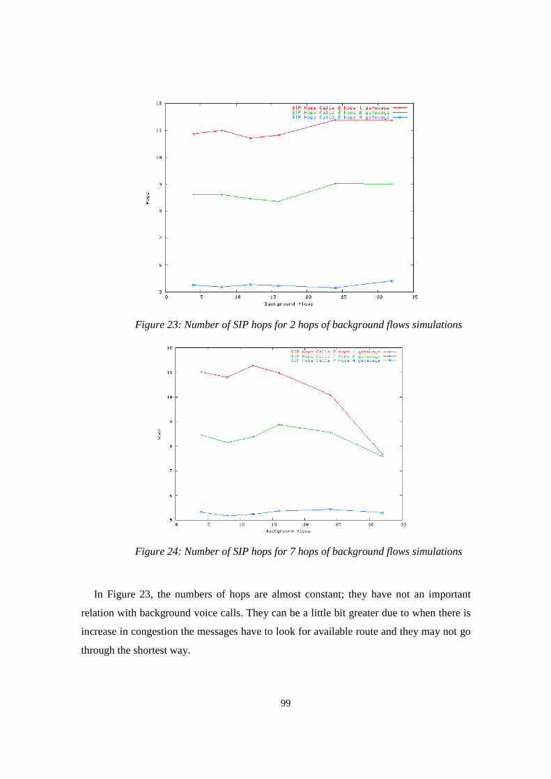
99
Figure 23: Number of SIP hops for 2 hops of background flows simulations
Figure 24: Number of SIP hops for 7 hops of background flows simulations
In Figure 23, the numbers of hops are almost constant; they have not an important
relation with background voice calls. They can be a little bit greater due to when there is
increase in congestion the messages have to look for available route and they may not go
through the shortest way.

100
However the most important information or conclusion from Figure 23 is how much
increasing the number of gateways can help to the network performance. When the
simulations work with one gateway, the SIP messages have to go through around 11 hops
and when 4 gateways are involved, these 11 hops may be reduced to 5 hops.
In Figure 24, the number of hops of one gateway and 32 background flows simulations
is very low. The call block probability of this simulation shown in Table 12 is 0.95, so
only 5 calls of 100 are established. These are the calls with the shortest distance between
caller and called, so the average of these number of hops is very low.
This information is very relevant to the whole network group of performance
parameters. Increasing the number of gateways is probably the most important factor in
improving the network performance parameters. It is obvious that having more gateways,
the congestion in and around the gateways is lower, if increased further, the number of
hops of traffic which go outside can be reduced up to half. It is also important for the call
block probability (reducing the number of hops by half should reduce the delay and the
number of dropped messages) and therefore for invitation attempts.
5.3.2 Evaluation of Voice Quality
To evaluate the voice quality, some performance parameters have to be evaluated.
Packet lost rate (4.5.1.4) and average end-to-emd delay of all packets (4.5.1.1) are used to
analyze the voice quality of background flows.
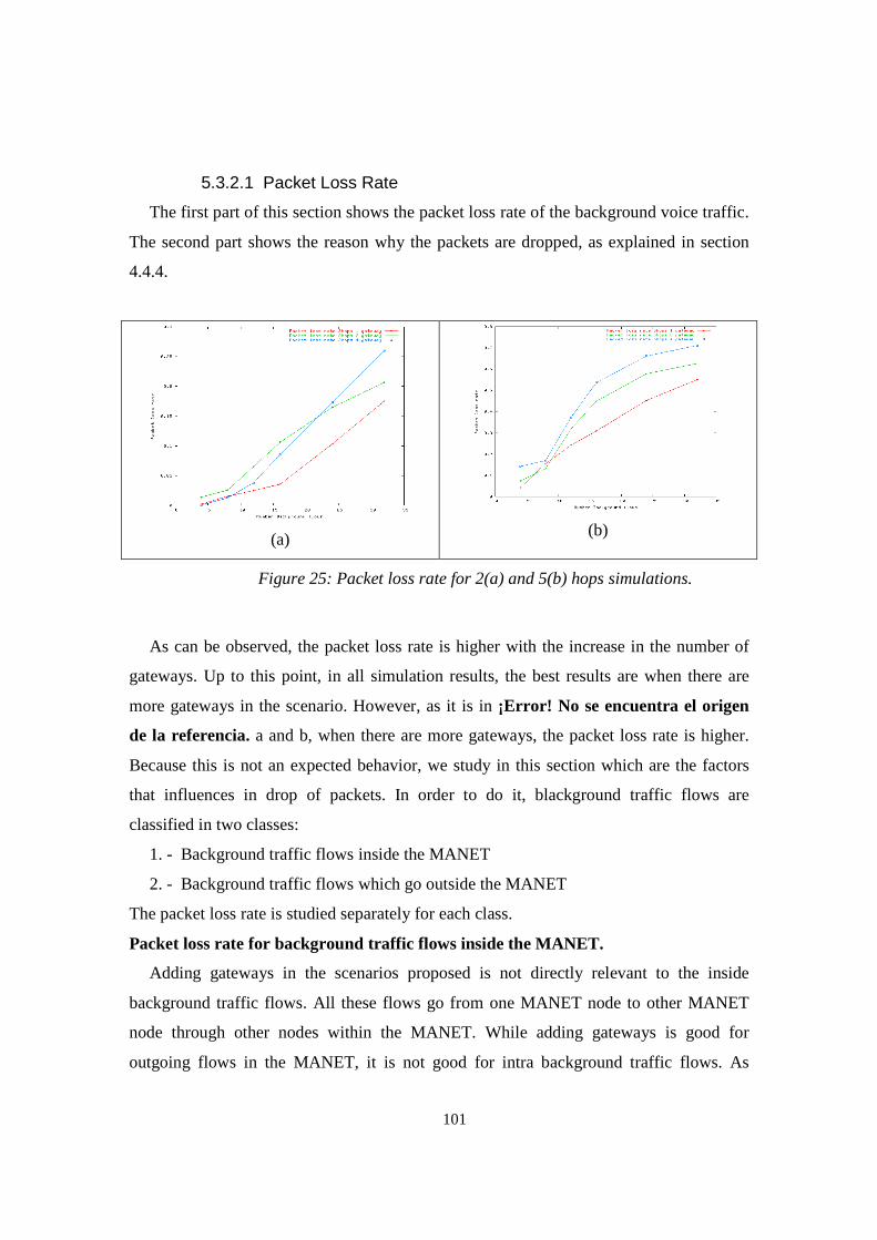
101
5.3.2.1 Packet Loss Rate
The first part of this section shows the packet loss rate of the background voice traffic.
The second part shows the reason why the packets are dropped, as explained in section
4.4.4.
(a)
(b)
Figure 25: Packet loss rate for 2(a) and 5(b) hops simulations.
As can be observed, the packet loss rate is higher with the increase in the number of
gateways. Up to this point, in all simulation results, the best results are when there are
more gateways in the scenario. However, as it is in ¡Error! No se encuentra el origen
de la referencia. a and b, when there are more gateways, the packet loss rate is higher.
Because this is not an expected behavior, we study in this section which are the factors
that influences in drop of packets. In order to do it, blackground traffic flows are
classified in two classes:
1. - Background traffic flows inside the MANET
2. - Background traffic flows which go outside the MANET
The packet loss rate is studied separately for each class.
Packet loss rate for background traffic flows inside the MANET.
Adding gateways in the scenarios proposed is not directly relevant to the inside
background traffic flows. All these flows go from one MANET node to other MANET
node through other nodes within the MANET. While adding gateways is good for
outgoing flows in the MANET, it is not good for intra background traffic flows. As
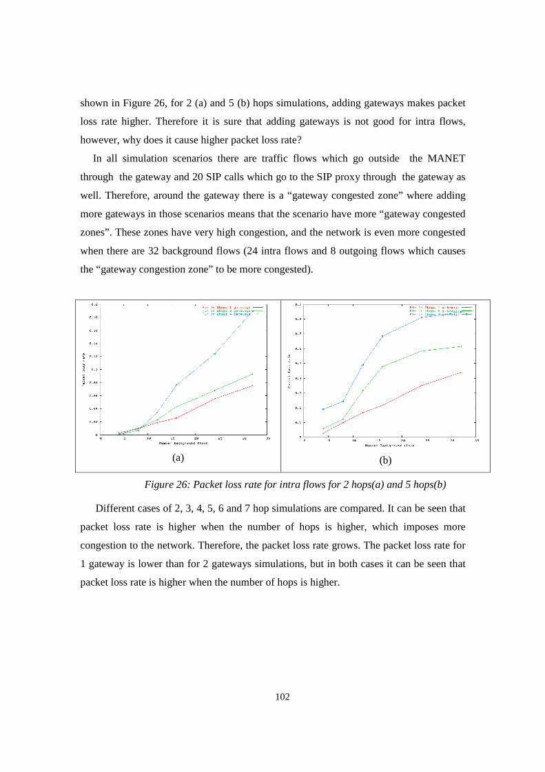
102
shown in Figure 26, for 2 (a) and 5 (b) hops simulations, adding gateways makes packet
loss rate higher. Therefore it is sure that adding gateways is not good for intra flows,
however, why does it cause higher packet loss rate?
In all simulation scenarios there are traffic flows which go outside the MANET
through the gateway and 20 SIP calls which go to the SIP proxy through the gateway as
well. Therefore, around the gateway there is a “gateway congested zone” where adding
more gateways in those scenarios means that the scenario have more “gateway congested
zones”. These zones have very high congestion, and the network is even more congested
when there are 32 background flows (24 intra flows and 8 outgoing flows which causes
the “gateway congestion zone” to be more congested).
(a)
(b)
Figure 26: Packet loss rate for intra flows for 2 hops(a) and 5 hops(b)
Different cases of 2, 3, 4, 5, 6 and 7 hop simulations are compared. It can be seen that
packet loss rate is higher when the number of hops is higher, which imposes more
congestion to the network. Therefore, the packet loss rate grows. The packet loss rate for
1 gateway is lower than for 2 gateways simulations, but in both cases it can be seen that
packet loss rate is higher when the number of hops is higher.

103
Packet loss rate for outgoing background flows the MANET.
While adding gateways makes the packet loss rate higher for intra flows, there is a
different behavior for outgoing traffic flows. To discuss outgoing traffic flows, it is
important to mention the following , as stated in point 5.2.1 (Background Traffic
Scenario), the number of hops between MANET source and gateways is defined only
when the scenario has one gateway. After running such simulation (one gateway
simulation), this gateway is replaced by two and four gateways, but the MANET
source/destination remains at the same position.
The two hops simulation’s behavior is different and it can be seen in Figure 27 that
when the same simulation is run with two gateways, the number of hops for those
outgoing flows is greater than when there is only one gateway. If the same simulation is
run in four gateways scenario, the number of hops is practically the same as the number
of hops in one gateway scenario.
(a)
(b)
(c)
Figure 27: Outgoing traffic nodes for two hops simulations
For three hops, the distance between source and destination for outgoing traffic flows
is bigger in two gateways scenarios than in 4 gateways scenarios.
However for four or more hops simulations, increasing the number of gateways make
the number of hops between sources and gateways smaller. For six hops simulations,
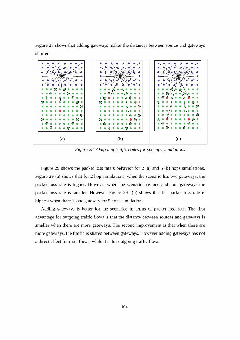
104
Figure 28 shows that adding gateways makes the distances between source and gateways
shorter.
(a)
(b)
(c)
Figure 28: Outgoing traffic nodes for six hops simulations
Figure 29 shows the packet loss rate’s behavior for 2 (a) and 5 (b) hops simulations.
Figure 29 (a) shows that for 2 hop simulations, when the scenario has two gateways, the
packet loss rate is higher. However when the scenario has one and four gateways the
packet loss rate is smaller. However Figure 29 (b) shows that the packet loss rate is
highest when there is one gateway for 5 hops simulations.
Adding gateways is better for the scenarios in terms of packet loss rate. The first
advantage for outgoing traffic flows is that the distance between sources and gateways is
smaller when there are more gateways. The second improvement is that when there are
more gateways, the traffic is shared between gateways. However adding gateways has not
a direct effect for intra flows, while it is for outgoing traffic flows.

105
(a)
(b)
Figure 29:Packet loss rate for outgoing flows for 2(a) and 5(b) hops
As conclusion, Figure 30 shows the packet loss rate for intra, outgoing and average of
all traffic flows. Figure 30 (a) shows the values for one gateway simulation and Figure 30
(b) shows the values for four gateways simulation, both within 5 hops scenarios.
When there is only one gateway, packet loss rate is higher for outgoing traffic flows
and when there are four gateways, packet loss rate is higher for intra traffic flows. The
average is always more similar to intra flows than to outgoing traffic flows. This is
because the proportion of intra to outgoing traffic flows is 3:1.
(a)
(b)
Figure 30:Packet loss rate for intra and outgoing flows for 1(a) and 4(b)
gateways and 5hops simulations
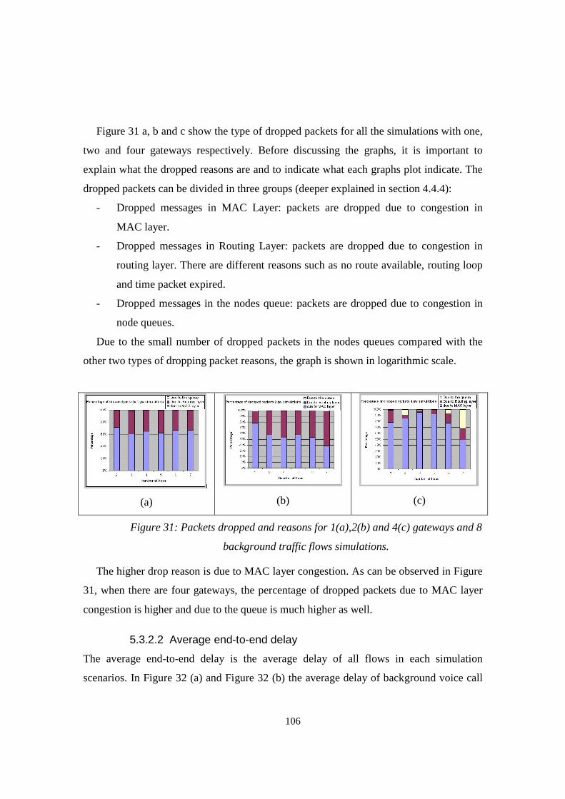
106
Figure 31 a, b and c show the type of dropped packets for all the simulations with one,
two and four gateways respectively. Before discussing the graphs, it is important to
explain what the dropped reasons are and to indicate what each graphs plot indicate. The
dropped packets can be divided in three groups (deeper explained in section 4.4.4):
- Dropped messages in MAC Layer: packets are dropped due to congestion in
MAC layer.
- Dropped messages in Routing Layer: packets are dropped due to congestion in
routing layer. There are different reasons such as no route available, routing loop
and time packet expired.
- Dropped messages in the nodes queue: packets are dropped due to congestion in
node queues.
Due to the small number of dropped packets in the nodes queues compared with the
other two types of dropping packet reasons, the graph is shown in logarithmic scale.
(a)
(b)
(c)
Figure 31: Packets dropped and reasons for 1(a),2(b) and 4(c) gateways and 8
background traffic flows simulations.
The higher drop reason is due to MAC layer congestion. As can be observed in Figure
31, when there are four gateways, the percentage of dropped packets due to MAC layer
congestion is higher and due to the queue is much higher as well.
5.3.2.2 Average end-to-end delay
The average end-to-end delay is the average delay of all flows in each simulation
scenarios. In Figure 32 (a) and Figure 32 (b) the average delay of background voice call
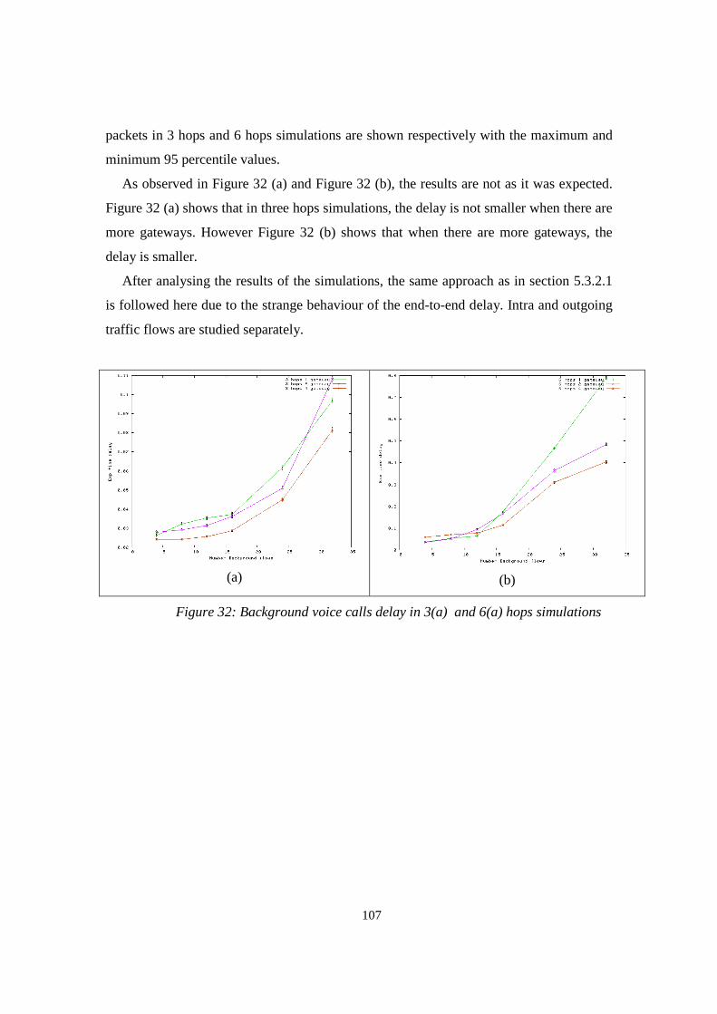
107
packets in 3 hops and 6 hops simulations are shown respectively with the maximum and
minimum 95 percentile values.
As observed in Figure 32 (a) and Figure 32 (b), the results are not as it was expected.
Figure 32 (a) shows that in three hops simulations, the delay is not smaller when there are
more gateways. However Figure 32 (b) shows that when there are more gateways, the
delay is smaller.
After analysing the results of the simulations, the same approach as in section 5.3.2.1
is followed here due to the strange behaviour of the end-to-end delay. Intra and outgoing
traffic flows are studied separately.
(a)
(b)
Figure 32: Background voice calls delay in 3(a) and 6(a) hops simulations
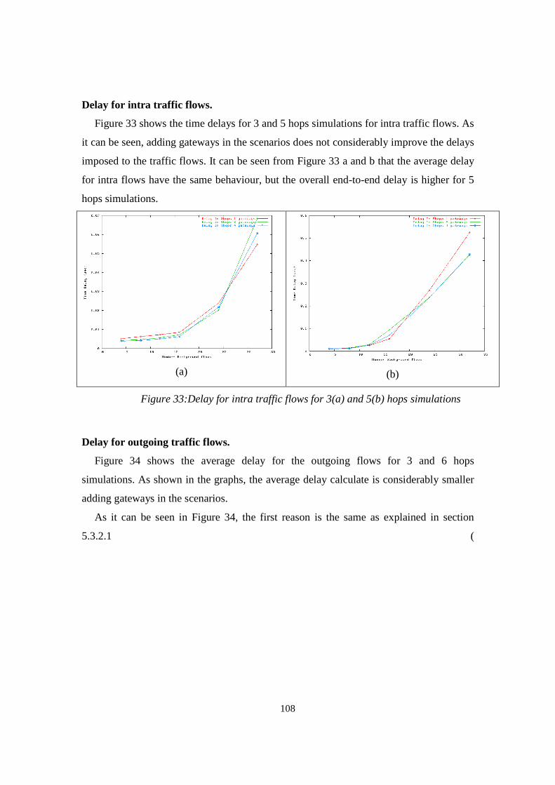
108
Delay for intra traffic flows.
Figure 33 shows the time delays for 3 and 5 hops simulations for intra traffic flows. As
it can be seen, adding gateways in the scenarios does not considerably improve the delays
imposed to the traffic flows. It can be seen from Figure 33 a and b that the average delay
for intra flows have the same behaviour, but the overall end-to-end delay is higher for 5
hops simulations.
(a)
(b)
Figure 33:Delay for intra traffic flows for 3(a) and 5(b) hops simulations
Delay for outgoing traffic flows.
Figure 34 shows the average delay for the outgoing flows for 3 and 6 hops
simulations. As shown in the graphs, the average delay calculate is considerably smaller
adding gateways in the scenarios.
As it can be seen in Figure 34, the first reason is the same as explained in section
5.3.2.1 (
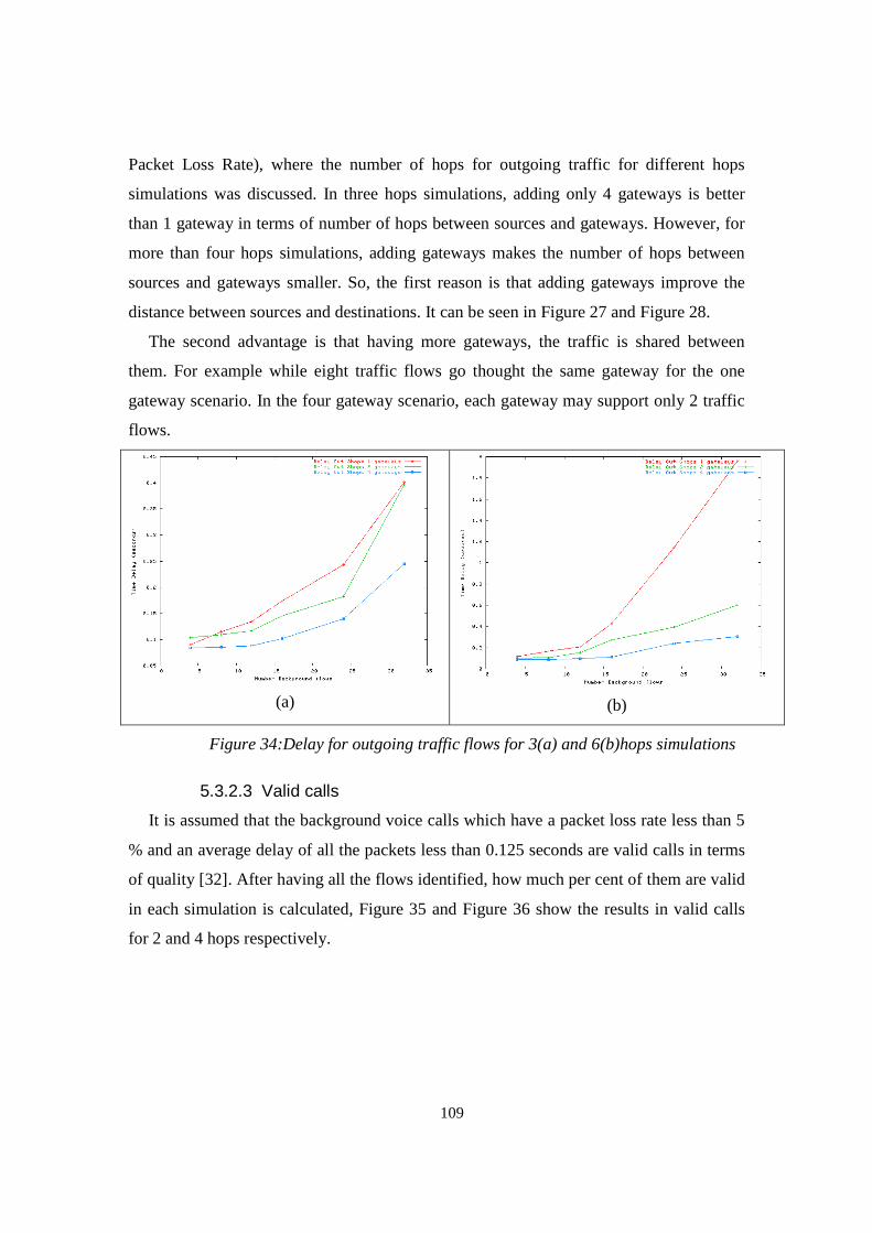
109
Packet Loss Rate), where the number of hops for outgoing traffic for different hops
simulations was discussed. In three hops simulations, adding only 4 gateways is better
than 1 gateway in terms of number of hops between sources and gateways. However, for
more than four hops simulations, adding gateways makes the number of hops between
sources and gateways smaller. So, the first reason is that adding gateways improve the
distance between sources and destinations. It can be seen in Figure 27 and Figure 28.
The second advantage is that having more gateways, the traffic is shared between
them. For example while eight traffic flows go thought the same gateway for the one
gateway scenario. In the four gateway scenario, each gateway may support only 2 traffic
flows.
(a)
(b)
Figure 34:Delay for outgoing traffic flows for 3(a) and 6(b)hops simulations
5.3.2.3 Valid calls
It is assumed that the background voice calls which have a packet loss rate less than 5
% and an average delay of all the packets less than 0.125 seconds are valid calls in terms
of quality [32]. After having all the flows identified, how much per cent of them are valid
in each simulation is calculated, Figure 35 and Figure 36 show the results in valid calls
for 2 and 4 hops respectively.
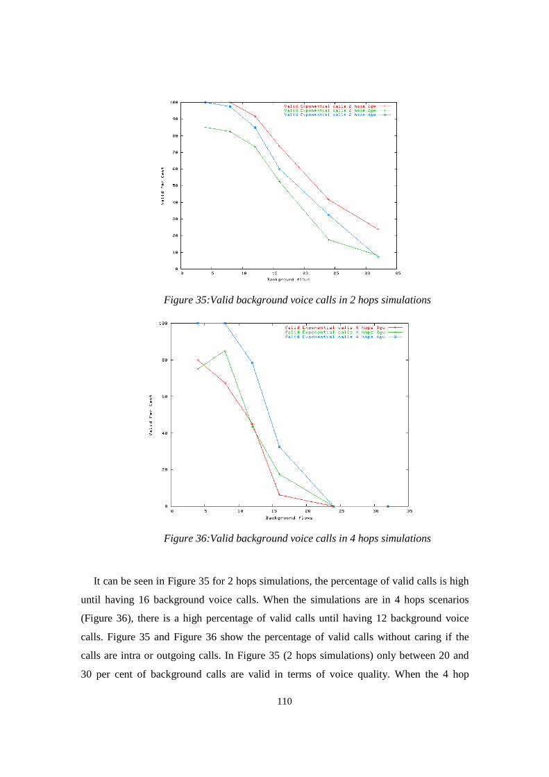
110
Figure 35:Valid background voice calls in 2 hops simulations
Figure 36:Valid background voice calls in 4 hops simulations
It can be seen in Figure 35 for 2 hops simulations, the percentage of valid calls is high
until having 16 background voice calls. When the simulations are in 4 hops scenarios
(Figure 36), there is a high percentage of valid calls until having 12 background voice
calls. Figure 35 and Figure 36 show the percentage of valid calls without caring if the
calls are intra or outgoing calls. In Figure 35 (2 hops simulations) only between 20 and
30 per cent of background calls are valid in terms of voice quality. When the 4 hop

111
scenarios are assumed (Figure 36), it is not possible to have more than 16 background
voice calls.
Table 13 and Table 14 show the average values of (PLR) Packet Loss Rate and end-to-
end delay of background traffic packets for 2 and 5 hops simulations respectively. The
row “Valids %” represents the percentage of valid background calls in terms of packet
loss rate and delay as it was stated at the beginning of this section (PLR < 5% and end-to-
end delay < 0.125 seconds).
As can be seen, there are much higher percentage of valid calls for two hops
simulations mainly because of fewer packet dropped compared to the scenario with 5
hops. It can be seen that adding gateways improves the percentage of valid calls.
According to Table 13 and Table 14, it is also true that Packet Loss Rate has a higher
influence in the voice quality analysis, compared to end-to-end delay.
2 hops 1 gateway
N flows 4 8 12 16 24 32
PLR 0.0021 0.015 0.025 0.035 0.103 0.175
DELAY 0.0243 0.027 0.028 0.03 0.058 0.092
Valids % 100 100 91.6 73 41 23.75
2 hops 2 gateways
N flows 4 8 12 16 24 32
PLR 0.0142 0.026 0.065 0.106 0.165 0.207
DELAY 0.0255 0.026 0.032 0.043 0.061 0.095
Valids % 85 82.5 73 52 17.5 8.125
2 hops 4 gateways
N flows 4 8 12 16 24 32
PLR 0.0003 0.012 0.038 0.085 0.173 0.26
DELAY 0.0224 0.024 0.025 0.028 0.045 0.068
Valids % 100 97 85 60 32 6.875
Table 13: Valid background calls for 2 hops simulations
5 hops 1 gateway
N flows 4 8 12 16 24 32
PLR 0.042 0.156 0.243 0.308 0.453 0.55
DELAY 0.034 0.047 0.065 0.1 0.382 0.709
Valids % 75 2.5 0 0 0 0
5 hops 2 gateways
N flows 4 8 12 16 24 32
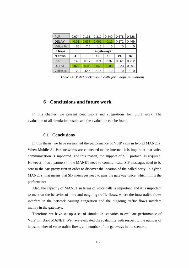
112
PLR 0.074 0.131 0.319 0.449 0.578 0.626
DELAY 0.03 0.037 0.062 0.12 0.272 0.469
Valids % 65 7.5 1.6 0 0 0
5 hops 4 gateways
N flows 4 8 12 16 24 32
PLR 0.143 0.17 0.374 0.537 0.661 0.712
DELAY 0.029 0.03 0.043 0.08 0.23 0.391
Valids % 70 42.5 21.5 10 0 0
Table 14: Valid background calls for 5 hops simulations
6 Conclusions and future work
In this chapter, we present conclusions and suggestions for future work. The
evaluation of all simulation results and the evaluation can be found.
6.1 Conclusions
In this thesis, we have researched the performance of VoIP calls in hybrid MANETs.
When Mobile Ad Hoc networks are connected to the internet, it is important that voice
communication is supported. For this reason, the support of SIP protocol is required.
However, if two partners in the MANET need to communicate, SIP messages need to be
sent to the SIP proxy first in order to discover the location of the called party. In hybrid
MANETs, that means that SIP messages need to pass the gateway twice, which limits the
performance.
Also, the capacity of MANET in terms of voice calls is important, and it is important
to mention the behavior of intra and outgoing traffic flows, where the intra traffic flows
interfere in the network causing congestion and the outgoing traffic flows interfere
mainly in the gateways.
Therefore, we have set up a set of simulation scenarios to evaluate performance of
VoIP in hybrid MANET. We have evaluated the scalability with respect to the number of
hops, number of voice traffic flows, and number of the gateways in the scenario,
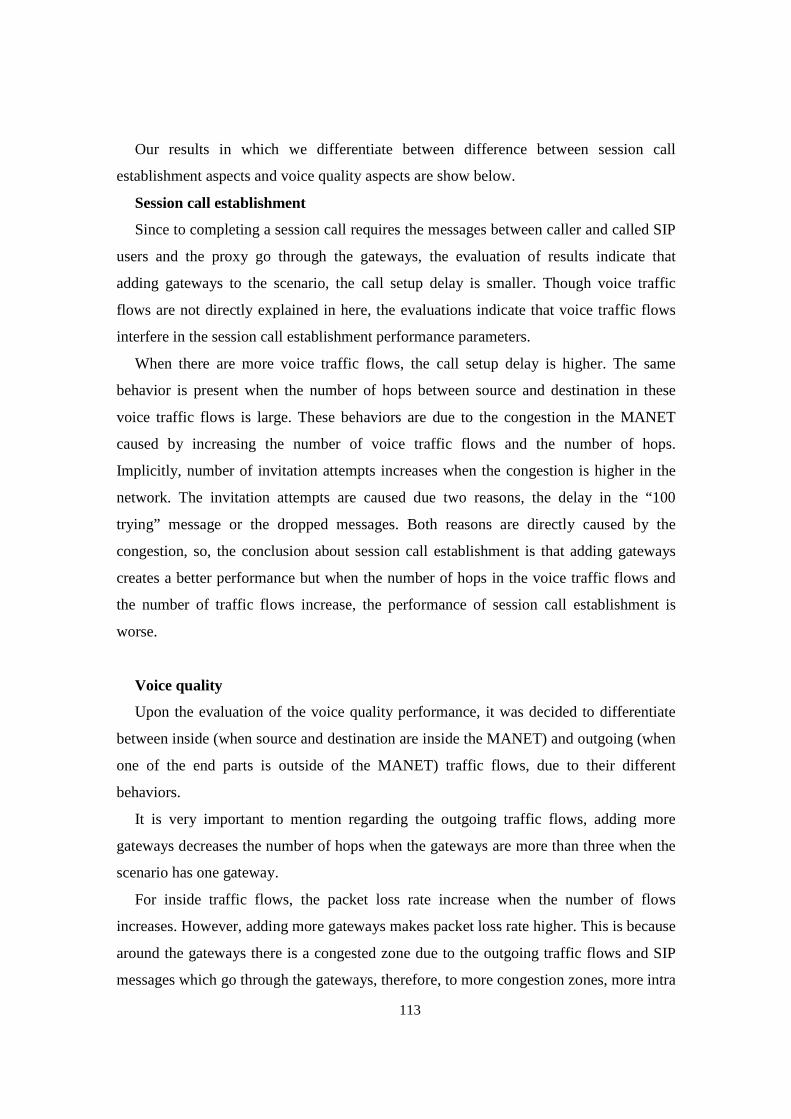
113
Our results in which we differentiate between difference between session call
establishment aspects and voice quality aspects are show below.
Session call establishment
Since to completing a session call requires the messages between caller and called SIP
users and the proxy go through the gateways, the evaluation of results indicate that
adding gateways to the scenario, the call setup delay is smaller. Though voice traffic
flows are not directly explained in here, the evaluations indicate that voice traffic flows
interfere in the session call establishment performance parameters.
When there are more voice traffic flows, the call setup delay is higher. The same
behavior is present when the number of hops between source and destination in these
voice traffic flows is large. These behaviors are due to the congestion in the MANET
caused by increasing the number of voice traffic flows and the number of hops.
Implicitly, number of invitation attempts increases when the congestion is higher in the
network. The invitation attempts are caused due two reasons, the delay in the “100
trying” message or the dropped messages. Both reasons are directly caused by the
congestion, so, the conclusion about session call establishment is that adding gateways
creates a better performance but when the number of hops in the voice traffic flows and
the number of traffic flows increase, the performance of session call establishment is
worse.
Voice quality
Upon the evaluation of the voice quality performance, it was decided to differentiate
between inside (when source and destination are inside the MANET) and outgoing (when
one of the end parts is outside of the MANET) traffic flows, due to their different
behaviors.
It is very important to mention regarding the outgoing traffic flows, adding more
gateways decreases the number of hops when the gateways are more than three when the
scenario has one gateway.
For inside traffic flows, the packet loss rate increase when the number of flows
increases. However, adding more gateways makes packet loss rate higher. This is because
around the gateways there is a congested zone due to the outgoing traffic flows and SIP
messages which go through the gateways, therefore, to more congestion zones, more intra

114
traffic flows badly influenced. Around these congested zones, the nodes suffer from
congestion problems, so the packet loss rate is higher when there are more gateways.
For outgoing voice traffic flows the behavior is totally different, packet loss rate is
lower due two reasons; the traffic that each gateway supports is lower and the distance in
number of hops between nodes and gateways is usually smaller.
The average end to end delay of the packets for intra flows has no significant
improvement by adding gateways. For outgoing flows, adding gateways improves
significantly the end-to-end delay.
As a conclusion, it can be said that adding gateways create a congested zones but it
gives a better performance in general.
6.2 Future work
In future work, next points explain briefly what we plan:
The first suggestion is to introduce mobility into the scenarios. In this thesis, all the
simulations have been run in static scenarios with one, two and four gateways. It would
be interesting to study the performance of the same parameters varying the mobility of
normal nodes and nodes acting as gateways. With this approach, mobile IP or any
mobility management protocol will be required.
The second suggestion tries to implement session initiation protocol (SIP) totally
inside a MANET that means, the caller, the callee and the SIP proxies are nodes in a
MANET. Several approaches can be applied:
One suggestion is trying to make the gateways acting as SIP proxies, if
there are gateways in the MANET.
The second suggestion does not need to have gateways in the MANET. The
approach can be making the SIP callers act as SIP proxy as well. For that, one
solution can be that all the SIP user nodes send register event to all the
MANET nodes.
The third suggestion tries to solve some problems encountered in this thesis with the
SIP protocol. As it was commented when call block probability was evaluated, SIP proxy
has vulnerability when some packets are dropped.

115
When the “200 ok” message from the called node to the proxy is dropped, the call will
never be established. The internal reason of this is because when the called node sends
the invitation acceptance, this node goes into “busy” state, and when a node is in “busy”
state, it can not listen one invitation. So if the acceptance message is dropped, the call
will never be established.
There can be many ways to solve this problem; the next ones can be some suggestions:
The node can send more acceptance messages after a while, until the call is
established.
The called node can identify which the caller node is; therefore, if the caller
node wants to send another invitation because it did not receive the acceptance,
the called node can receive and consider another invitation in “busy” state if
the invitation is from the same caller node which made being in “busy” state.
The fourth suggestion is use MAC protocol 802.11e with Quality of Service, where
SIP and routing messages will have High Priority. The expected results is that the call
establishment will improve while the voice quality will continue being poor.
116
References
[1] Nico Bayera, Bangnan Xua, Sven Hischkeb. An Architecture for connecting Ad hoc Networks with the IPv6 Backbone (6Bone) using a Wireless Gateway.
[2] Jin Xi and Christian Bettstetter. Wireless Multihop Internet access: Gateway discovery, routing and addressing. Technische Universität München.
[3] Alex Ali Hamidian. A Study of Internet Connectivity for Mobile Ad Hoc Networks in NS 2.
[4] Pedro M. Ruiz, Antonio F. Gomez-Skarmeta. Adaptive Gateway Discovery Mechanisms to Enhance Internet Connectivity for Mobile Ad Hoc Networks.
[5] C.Siva Murthy and B. S. Manoj. Ad Hoc Wireless Networks Architectures and Protocols.
[6] Abraham Silberschatz and Peter B. Galvin. Operatin system Concepts. Addison Wesley, 4th edition, 1994.
[7] Björn Wigerg. Porting AODV-UU Implementation to ns-2 and Enabling Trace-Based Simulation. Uppsala University, December 2002.
[8] NS-2 Trace Formats. http://www.grc.upv.es/manets/local/docs/griswoldNS-2%20Traces.htm
[9] Larry Wall, Tom Christiansen & Randal L. Schwartz. Programming Perl. Second Edition, September 1996.
[10] Christer Ahlund. Extended Mobile IP and support for Global Connectivity in Hybrid Networks. Lulea university, May 2005.
[11] Alba Batlle Linares and Jonas Karlsson. Evaluation of TCP Performance in hybrid Mobile Ad Hoc Networks. Karlstad University, June, 2006.
[12] Erik Nordstrom, Per Gunningberg, Christian Tschudin. Comparison of forwarding Strategies in Internet Connected MANETS. Uppsala University.
[13] Tuulia Kullberg. Performance of the Ad Hoc On Demand Distance Vector Routing Protocol. Helsinki University.
[14] Urban Olofsson and Rickard Sjöström. A prototype for Extending Global IP Connectivity for Ad Hoc Networks. October 2004.
[15] Alexander Zurkinden. Performance Evaluation of AODV Routing Protocol. June 2003.
[16] Gonzalo Camarillo. SIP Desmitified. Mac Grill, 2002.
[17] Dorgham Sisalem Jiri Kuthan. Galvin. Sip tutorial. Mobile Integrated Services.
[18] Alan B. Johnston. Sip: understanding the Session Initiation Protocol. Artech House Boston, second edition, 2004.
[19] Radvision, the VOIP experts. Understanding SIP Servers. Radvision, August, 2002.
[20] Fredrik Thernelius. SIP,NAT, and Firewalls. May, 2000.
[21] K. Fall, K. Varadhan. The ns manual (formely ns Notes and Documentation). http://www.isi.edu/nsnam/ns/ns-documentation.html April 2006.

117
[22] Jae Chung , Mark Claypool. Ns by example. Worcester Polytechnic Institute. http://nile.wpi.edu/NS/
[23] A. Triviño-Cabrera, E. Casilari-Pérez, A. Ariza-Quintana. Implementación de protocolos en el Network Simulator. Universidad de Malaga
[24] Marc Greis. Tutorial fot the Network Simulator “ns”. VINT group.
[25] Eitan Altman and Tania Jiménez. Venezuela. NS Simulator for beginners, December ,2003
[26] The Network Simulator. Universidad de la República. Uruguay
[27] Enrico Minack. Evaluation of the influence channel conditions on Car2X Communication. November, 2005.Chemnitz University of Technology.
[28] ITU-T Recommendation P.59, “Artificial conversational speech”, 1993
[29] ITU-T Recommendation Recommendation E.721,May, 1999.
[30] Enrico Minack “Evaluation of the influence of channel conditions on Car2X Communication” November 2005.
[31] http://www.tkn.tu-berlin.de/research/802.11e_ns2/techreport.pdf.
[32] Dragos Niculescu, Samrat Ganguly, Kyungtae Kim, Rauf Izmailov
“Performance of VoIP in a 802.11 Wireless Mesh Network”
[33] Perkins, C. & Bhagwat, P. (1994) Highly dynamic destination-sequenced distance-vector routing (DSDV) for mobile computers.
[34] Ilyas, M. (2003). The Handbook of Ad Hoc Wireless Networks
[35] Johnson, D. & Maltz, D. & Broch, J.DSR: The Dynamic Source Routing Protocol for Multi-Hop Wireless Ad Hoc Networks
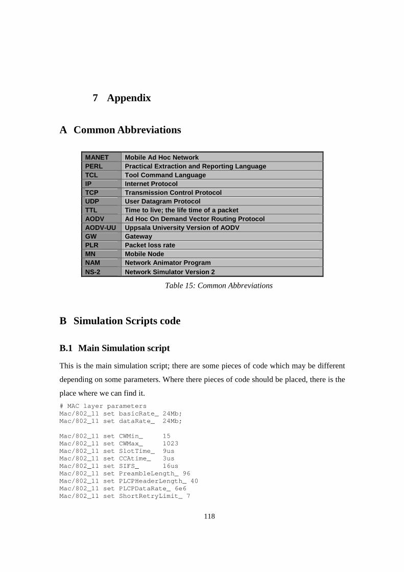
118
7 Appendix
A Common Abbreviations
MANET Mobile Ad Hoc Network PERL Practical Extraction and Reporting Language TCL Tool Command Language IP Internet Protocol TCP Transmission Control Protocol UDP User Datagram Protocol TTL Time to live; the life time of a packet AODV Ad Hoc On Demand Vector Routing Protocol AODV-UU Uppsala University Version of AODV GW Gateway PLR Packet loss rate MN Mobile Node NAM Network Animator Program NS-2 Network Simulator Version 2
Table 15: Common Abbreviations
B Simulation Scripts code
B.1 Main Simulation script
This is the main simulation script; there are some pieces of code which may be different
depending on some parameters. Where there pieces of code should be placed, there is the
place where we can find it.
# MAC layer parameters Mac/802_11 set basicRate_ 24Mb; Mac/802_11 set dataRate_ 24Mb; Mac/802_11 set CWMin_ 15 Mac/802_11 set CWMax_ 1023 Mac/802_11 set SlotTime_ 9us Mac/802_11 set CCAtime_ 3us Mac/802_11 set SIFS_ 16us Mac/802_11 set PreambleLength_ 96 Mac/802_11 set PLCPHeaderLength_ 40 Mac/802_11 set PLCPDataRate_ 6e6 Mac/802_11 set ShortRetryLimit_ 7
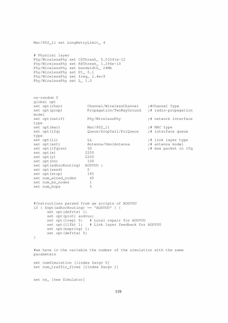
119
Mac/802_11 set LongRetryLimit_ 4 # Physical layer Phy/WirelessPhy set CSThresh_ 5.53241e-12 Phy/WirelessPhy set RXThresh_ 1.296e-10 Phy/WirelessPhy set bandwidth_ 24Mb Phy/WirelessPhy set Pt_ 0.1 Phy/WirelessPhy set freq_ 2.4e+9 Phy/WirelessPhy set L_ 1.0 ns-random 0 global opt set opt(chan) Channel/WirelessChannel ;#Channel Type set opt(prop) Propagation/TwoRayGround ;# radio-propagation model set opt(netif) Phy/WirelessPhy ;# network interface type set opt(mac) Mac/802_11 ;# MAC type set opt(ifq) Queue/DropTail/PriQueue ;# interface queue type set opt(ll) LL ;# link layer type set opt(ant) Antenna/OmniAntenna ;# antenna model set opt(ifqlen) 50 ;# max packet in ifq set opt(x) 2200 set opt(y) 2200 set opt(nn) 100 set opt(adhocRouting) AODVUU ; set opt(seed) 0 set opt(stop) 185 set num_wired_nodes 45 set num_bs_nodes 1 set num_hops 5 #Instructions parsed from gw scripts of AODVUU if { $opt(adhocRouting) == "AODVUU" } { set opt(defrte) 1; set opt(prot) aodvuu; set opt(lrep) 0; # Local repair for AODVUU set opt(llfb) 1; # Link layer feedback for AODVU U set opt(expring) 1; set opt(defrte) 0; } #we have in the variable the number of the simulati on with the same parameters set numSimulation [lindex $argv 0] set num_traffic_flows [lindex $argv 1] set ns_ [new Simulator]
120
# set up for hierarchical routing $ns_ node-config -addressType hierarchical AddrParams set domain_num_ 2 lappend cluster_num 1 1 AddrParams set cluster_num_ $cluster_num lappend eilastlevel 46 107 AddrParams set nodes_num_ $eilastlevel set tracefd [open traceFile-num:$numSimulation-gw: $num_bs_nodes-hops:$num_hops-flows:$num_traffic_flows.tr w] $ns_ trace-all $tracefd # Create topography object set topo [new Topography] # Create channel #set chan_1_ [new $opt(chan)] # define topology $topo load_flatgrid $opt(x) $opt(y) # create God create-god [expr $opt(nn) + $num_bs_nodes] #create wired nodes #next code lines create 45 wired nodes for {set i 0} {$i < $num_wired_nodes} {incr i} { set W($i) [$ns_ node 0.0.$i] } # configure for base-station node $ns_ node-config -adhocRouting $opt(adhocRouting) \ -llType $opt(ll) \ -macType $opt(mac) \ -ifqType $opt(ifq) \ -ifqLen $opt(ifqlen) \ -antType $opt(ant) \ -propType $opt(prop) \ -phyType $opt(netif) \ -channelType $opt(chan) \ -topoInstance $topo \ -wiredRouting ON \ -agentTrace ON \ -routerTrace OFF \ -macTrace OFF #------------------------------------------------ #------------------------------------------------ # here it should be the gateways/base stations defi nition # this definition is different depending on the num ber of gateways # the different gateways definitions are in appendi x B.1.1 #------------------------------------------------ #------------------------------------------------

121
#configure for mobilenodes $ns_ node-config -wiredRouting OFF for {set j 0} {$j < $opt(nn)} {incr j} { if {$j != 54 } { set node_($j) [ $ns_ node 1.0.$j ] $node_($j) base-station [AddrParams addr2id \ [$BS(0) node-addr]] set posicion_x [expr ($j % 10) * 200 ] set posicion_y [expr ($j / 10) * 200 ] $node_($j) set X_ $posicion_x $node_($j) set Y_ $posicion_y $node_($j) set Z_ 0.0 } } #create links between wired and BS nodes for {set x 1} {$x < $num_wired_nodes} {incr x} { $ns_ duplex-link $W(0) $W($x) 5Mb 40ms DropTail } $ns_ duplex-link $W(0) $BS(0) 5Mb 40ms DropTail puts "-------Identifiers of the nodes------" for {set x 0} {$x < $num_wired_nodes} {incr x} { puts "W($x) = [$W($x) node-addr] = [AddrParams addr2id [$W($x) node-addr]] node_id in the trace file = [$W($x) id] " } for {set x 0} {$x < $num_bs_nodes} {incr x} { puts "BS($x) = [$BS($x) node-addr] = [AddrPara ms addr2id [$BS($x) node-addr]] node_id in the trace file = [$BS($x) id ]" } for {set x 0} {$x < $opt(nn)} {incr x} { if {$x != 54 } { puts "node_($x) = [$node_($x) node-addr] = [Ad drParams addr2id [$node_($x) node-addr]] node_id in the trace file = [$node_($x) id]" } } #----------------------------------------------- #............SIP invitation calls............... #----------------------------------------------- # Proxy servers $W(0) label "proxy.atlanta.com" set serveraddrATL [$W(0) node-addr] set sipATL [new Agent/SIPProxy atlanta.com] $W(0) attach $sipATL 5 #---------------------------------------------- #------------ NODES in SIP calls --------- #---------------------------------------------- # here there are 40 wireless nodes , 20 caller node s and 20 called nodes # there are 5 groups of them, because there are 5 r epetitions of each simulation # we can see them in the appendix B.1.3

122
# User agents #there are 8 sip invitation calls #this is the first one $caller1 label "[email protected]" set sipalice1 [new Agent/SIPUA alice1 atlanta.com ] $caller1 attach $sipalice1 5 $invited1 label "[email protected]" set sipbob1 [new Agent/SIPUA bob1 atlanta.com] $invited1 attach $sipbob1 5 #this is the second one $caller2 label "[email protected]" set sipalice2 [new Agent/SIPUA alice2 atlanta.com ] $caller2 attach $sipalice2 5 $invited1 label "[email protected]" set sipbob2 [new Agent/SIPUA bob2 atlanta.com] $invited2 attach $sipbob2 5 #this is the third sip invitation call $caller3 label "[email protected]" set sipalice3 [new Agent/SIPUA alice3 atlanta.com ] $caller3 attach $sipalice3 5 $invited3 label "[email protected]" set sipbob3 [new Agent/SIPUA bob3 atlanta.com] $invited3 attach $sipbob3 5 #this is the forth sip invitation call $caller4 label "[email protected]" set sipalice4 [new Agent/SIPUA alice4 atlanta.com ] $caller4 attach $sipalice4 5 $invited4 label "[email protected]" set sipbob4 [new Agent/SIPUA bob4 atlanta.com] $invited4 attach $sipbob4 5 #this is the fifth sip invitation call $caller5 label "[email protected]" set sipalice5 [new Agent/SIPUA alice5 atlanta.com ] $caller5 attach $sipalice5 5 $invited5 label "[email protected]" set sipbob5 [new Agent/SIPUA bob5 atlanta.com] $invited5 attach $sipbob5 5 # this is the sixth sip invitation call $caller6 label "[email protected]" set sipalice6 [new Agent/SIPUA alice6 atlanta.com ] $caller6 attach $sipalice6 5 $invited6 label "[email protected]" set sipbob6 [new Agent/SIPUA bob6 atlanta.com] $invited6 attach $sipbob6 5 #this is the 7th sip invitation call $caller7 label "[email protected]" set sipalice7 [new Agent/SIPUA alice7 atlanta.com ] $caller7 attach $sipalice7 5 $invited7 label "[email protected]" set sipbob7 [new Agent/SIPUA bob7 atlanta.com] $invited7 attach $sipbob7 5 #this is the 8th sip invitation call $caller8 label "[email protected]" set sipalice8 [new Agent/SIPUA alice8 atlanta.com ] $caller8 attach $sipalice8 5 $invited8 label "[email protected]"
123
set sipbob8 [new Agent/SIPUA bob8 atlanta.com] $invited8 attach $sipbob8 5 $caller9 label "[email protected]" set sipalice9 [new Agent/SIPUA alice9 atlanta.com ] $caller9 attach $sipalice9 5 $invited9 label "[email protected]" set sipbob9 [new Agent/SIPUA bob9 atlanta.com] $invited9 attach $sipbob9 5 #this is the 10th one $caller10 label "[email protected]" set sipalice10 [new Agent/SIPUA alice10 atlanta.c om] $caller10 attach $sipalice10 5 $invited10 label "[email protected]" set sipbob10 [new Agent/SIPUA bob10 atlanta.com] $invited10 attach $sipbob10 5 #this is the 11th sip invitation call $caller11 label "[email protected]" set sipalice11 [new Agent/SIPUA alice11 atlanta.c om] $caller11 attach $sipalice11 5 $invited11 label "[email protected]" set sipbob11 [new Agent/SIPUA bob11 atlanta.com] $invited11 attach $sipbob11 5 #this is the 12th sip invitation call $caller12 label "[email protected]" set sipalice12 [new Agent/SIPUA alice12 atlanta.c om] $caller12 attach $sipalice12 5 $invited12 label "[email protected]" set sipbob12 [new Agent/SIPUA bob12 atlanta.com] $invited12 attach $sipbob12 5 #this is the 13th sip invitation call $caller13 label "[email protected]" set sipalice13 [new Agent/SIPUA alice13 atlanta.c om] $caller13 attach $sipalice13 5 $invited13 label "[email protected]" set sipbob13 [new Agent/SIPUA bob13 atlanta.com] $invited13 attach $sipbob13 5 # this is the 14 sip invitation call $caller14 label "[email protected]" set sipalice14 [new Agent/SIPUA alice14 atlanta.c om] $caller14 attach $sipalice14 5 $invited14 label "[email protected]" set sipbob14 [new Agent/SIPUA bob14 atlanta.com] $invited14 attach $sipbob14 5 #this is the 15th sip invitation call $caller15 label "[email protected]" set sipalice15 [new Agent/SIPUA alice15 atlanta.c om] $caller15 attach $sipalice15 5 $invited15 label "[email protected]" set sipbob15 [new Agent/SIPUA bob15 atlanta.com] $invited15 attach $sipbob15 5 #this is the 16th sip invitation call $caller16 label "[email protected]" set sipalice16 [new Agent/SIPUA alice16 atlanta.c om] $caller16 attach $sipalice16 5 $invited16 label "[email protected]" set sipbob16 [new Agent/SIPUA bob16 atlanta.com] $invited16 attach $sipbob16 5 $caller17 label "[email protected]"

124
set sipalice17 [new Agent/SIPUA alice17 atlanta.c om] $caller17 attach $sipalice17 5 $invited17 label "[email protected]" set sipbob17 [new Agent/SIPUA bob17 atlanta.com] $invited17 attach $sipbob17 5 $caller18 label "[email protected]" set sipalice18 [new Agent/SIPUA alice18 atlanta.c om] $caller18 attach $sipalice18 5 $invited18 label "[email protected]" set sipbob18 [new Agent/SIPUA bob18 atlanta.com] $invited18 attach $sipbob18 5 #this is the 19th sip invitation call $caller19 label "[email protected]" set sipalice19 [new Agent/SIPUA alice19 atlanta.c om] $caller19 attach $sipalice19 5 $invited19 label "[email protected]" set sipbob19 [new Agent/SIPUA bob19 atlanta.com] $invited19 attach $sipbob19 5 #this is the 20th sip invitation call $caller20 label "[email protected]" set sipalice20 [new Agent/SIPUA alice20 atlanta.c om] $caller20 attach $sipalice20 5 $invited20 label "[email protected]" set sipbob20 [new Agent/SIPUA bob20 atlanta.com] $invited20 attach $sipbob20 5 # Setup outbound proxies $sipalice1 set-proxy $serveraddrATL $sipbob1 set-proxy $serveraddrATL $sipalice2 set-proxy $serveraddrATL $sipbob2 set-proxy $serveraddrATL $sipalice3 set-proxy $serveraddrATL $sipbob3 set-proxy $serveraddrATL $sipalice4 set-proxy $serveraddrATL $sipbob4 set-proxy $serveraddrATL $sipalice5 set-proxy $serveraddrATL $sipbob5 set-proxy $serveraddrATL $sipalice6 set-proxy $serveraddrATL $sipbob6 set-proxy $serveraddrATL $sipalice7 set-proxy $serveraddrATL $sipbob7 set-proxy $serveraddrATL $sipalice8 set-proxy $serveraddrATL $sipbob8 set-proxy $serveraddrATL $sipalice9 set-proxy $serveraddrATL $sipbob9 set-proxy $serveraddrATL $sipalice10 set-proxy $serveraddrATL $sipbob10 set-proxy $serveraddrATL $sipalice11 set-proxy $serveraddrATL $sipbob11 set-proxy $serveraddrATL $sipalice12 set-proxy $serveraddrATL $sipbob12 set-proxy $serveraddrATL $sipalice13 set-proxy $serveraddrATL $sipbob13 set-proxy $serveraddrATL $sipalice14 set-proxy $serveraddrATL $sipbob14 set-proxy $serveraddrATL $sipalice15 set-proxy $serveraddrATL $sipbob15 set-proxy $serveraddrATL
125
$sipalice16 set-proxy $serveraddrATL $sipbob16 set-proxy $serveraddrATL $sipalice17 set-proxy $serveraddrATL $sipbob17 set-proxy $serveraddrATL $sipalice18 set-proxy $serveraddrATL $sipbob18 set-proxy $serveraddrATL $sipalice19 set-proxy $serveraddrATL $sipbob19 set-proxy $serveraddrATL $sipalice20 set-proxy $serveraddrATL $sipbob20 set-proxy $serveraddrATL # Set Record-Route on proxies $sipATL set recordRoute_ 1 #$sipBLX set recordRoute_ 1 # Register proxies with DNS "God" DNSGod register proxy atlanta.com $serveraddrATL #DNSGod register proxy biloxi.com $serveraddrBLX $ns_ at 1 "$ns_ trace-annotate \"Registering alices [email protected]\"" $ns_ at 1 "$sipalice1 register" $ns_ at 1 "$sipalice2 register" $ns_ at 1 "$sipalice3 register" $ns_ at 1 "$sipalice4 register" $ns_ at 1 "$sipalice5 register" $ns_ at 1 "$sipalice6 register" $ns_ at 1 "$sipalice7 register" $ns_ at 1 "$sipalice8 register" $ns_ at 1 "$sipalice9 register" $ns_ at 1 "$sipalice10 register" $ns_ at 1 "$sipalice11 register" $ns_ at 1 "$sipalice12 register" $ns_ at 1 "$sipalice13 register" $ns_ at 1 "$sipalice14 register" $ns_ at 1 "$sipalice15 register" $ns_ at 1 "$sipalice16 register" $ns_ at 1 "$sipalice17 register" $ns_ at 1 "$sipalice18 register" $ns_ at 1 "$sipalice19 register" $ns_ at 1 "$sipalice20 register" $ns_ at 1.1 "$ns_ trace-annotate \"Registering bobs [email protected]\"" $ns_ at 1.1 "$sipbob1 register" $ns_ at 1.1 "$sipbob2 register" $ns_ at 1.1 "$sipbob3 register" $ns_ at 1.1 "$sipbob4 register" $ns_ at 1.1 "$sipbob5 register" $ns_ at 1.1 "$sipbob6 register" $ns_ at 1.1 "$sipbob7 register" $ns_ at 1.1 "$sipbob8 register" $ns_ at 1.1 "$sipbob9 register" $ns_ at 1.1 "$sipbob10 register" $ns_ at 1.1 "$sipbob11 register" $ns_ at 1.1 "$sipbob12 register"

126
$ns_ at 1.1 "$sipbob13 register" $ns_ at 1.1 "$sipbob14 register" $ns_ at 1.1 "$sipbob15 register" $ns_ at 1.1 "$sipbob16 register" $ns_ at 1.1 "$sipbob17 register" $ns_ at 1.1 "$sipbob18 register" $ns_ at 1.1 "$sipbob19 register" $ns_ at 1.1 "$sipbob20 register" set u 170 # Sessions $ns_ at 20 "$ns_ trace-annotate \"aliceNodes@atlant a.com start session to [email protected]\"" $ns_ at 20 "$sipalice1 invite bob1 atlanta.com bw 3 2kb 64kb" $ns_ at 25 "$sipalice2 invite bob2 atlanta.com bw 3 2kb 64kb" $ns_ at 30 "$sipalice3 invite bob3 atlanta.com bw 3 2kb 64kb" $ns_ at 35 "$sipalice4 invite bob4 atlanta.com bw 3 2kb 64kb" $ns_ at 40 "$sipalice5 invite bob5 atlanta.com bw 3 2kb 64kb" $ns_ at 45 "$sipalice6 invite bob6 atlanta.com bw 3 2kb 64kb" $ns_ at 50 "$sipalice7 invite bob7 atlanta.com bw 3 2kb 64kb" $ns_ at 55 "$sipalice8 invite bob8 atlanta.com bw 3 2kb 64kb" $ns_ at 60 "$sipalice9 invite bob9 atlanta.com bw 3 2kb 64kb" $ns_ at 65 "$sipalice10 invite bob10 atlanta.com bw 32kb 64kb" $ns_ at 70 "$sipalice11 invite bob11 atlanta.com bw 32kb 64kb" $ns_ at 75 "$sipalice12 invite bob12 atlanta.com bw 32kb 64kb" $ns_ at 80 "$sipalice13 invite bob13 atlanta.com bw 32kb 64kb" $ns_ at 85 "$sipalice14 invite bob14 atlanta.com bw 32kb 64kb" $ns_ at 90 "$sipalice15 invite bob15 atlanta.com bw 32kb 64kb" $ns_ at 95 "$sipalice16 invite bob16 atlanta.com bw 32kb 64kb" $ns_ at 100 "$sipalice17 invite bob17 atlanta.com b w 32kb 64kb" $ns_ at 105 "$sipalice18 invite bob18 atlanta.com b w 32kb 64kb" $ns_ at 110 "$sipalice19 invite bob19 atlanta.com b w 32kb 64kb" $ns_ at 115 "$sipalice20 invite bob20 atlanta.com b w 32kb 64kb" $ns_ at $u "$ns_ trace-annotate \"bobsNodes@atlanta .com end session to [email protected] (any side may terminate the call)\"" $ns_ at $u "$sipbob1 bye" $ns_ at $u "$sipbob2 bye" $ns_ at $u "$sipbob3 bye" $ns_ at $u "$sipbob4 bye" $ns_ at $u "$sipbob5 bye" $ns_ at $u "$sipbob6 bye" $ns_ at $u "$sipbob7 bye" $ns_ at $u "$sipbob8 bye" $ns_ at $u "$sipbob9 bye" $ns_ at $u "$sipbob10 bye" $ns_ at $u "$sipbob11 bye" $ns_ at $u "$sipbob12 bye" $ns_ at $u "$sipbob13 bye" $ns_ at $u "$sipbob14 bye"

127
$ns_ at $u "$sipbob15 bye" $ns_ at $u "$sipbob16 bye" $ns_ at $u "$sipbob17 bye" $ns_ at $u "$sipbob18 bye" $ns_ at $u "$sipbob19 bye" $ns_ at $u "$sipbob20 bye" #----------------------------------------- # here we have the exponential traffic #----------------------------------------- # here there are 32 pairs of nodes, sources and des tinations # they are different depending on the number of hop s # we can see them in the appendix B.1.4 for {set i 0} {$i < $num_traffic_flows } {incr i} { ################## Traffic Agents for Applications ################### set src [new Agent/UDP] set sink [new Agent/Null] $ns_ attach-agent $sender($i) $src $ns_ attach-agent $receiver($i) $sink $ns_ connect $src $sink set e [new Application/Traffic/Exponential] $e attach-agent $src $e set packetSize_ 32 ;# corresponds to a filling time of about 20 ms for G729 $e set burst_time_ 350ms $e set idle_time_ 650ms $e set rate_ 12.8k ;# set src1 [new Agent/UDP] set sink1 [new Agent/Null] $ns_ attach-agent $receiver($i) $src1 $ns_ attach-agent $sender($i) $sink1 $ns_ connect $src1 $sink1 set e1 [new Application/Traffic/Exponential] $e1 attach-agent $src1 $e1 set packetSize_ 32 ;# corresponds to a filling time of about 20 ms for G729 $e1 set burst_time_ 350ms $e1 set idle_time_ 650ms $e1 set rate_ 12.8k ;#for G729 #Schedule events for the Exponential agents $ns_ at 5.0 "$e start" $ns_ at 5.1 "$e1 start" $ns_ at 185 "$e stop" $ns_ at 185 "$e1 stop" }

128
#----------------------------------------------- #----------------------------------------------- #Define a 'finish' procedure proc finish {} { global ns_ tracefd $ns_ flush-trace #Close the trace file close $tracefd exit 0 } # Tell all nodes when the simulation ends for {set i } {$i < $opt(nn) } {incr i} { if {$i != 54 } { $ns_ at $opt(stop).0 "$node_($i) reset"; } } $ns_ at $opt(stop).0 "$BS(0) reset"; $ns_ at 185 "puts \"NS EXITING...\" ; $ns_ halt" $ns_ at $opt(stop).0001 "finish" # informative headers for CMUTracefile set title "parameters:"; puts $tracefd "$title $numSimulation $num_bs_nodes $num_hops $num_traffic_flows " puts "Starting Simulation..." $ns_ run
B.1.1 Base station definition code
B.1.1.1 For one gateway
################ BASE STATION 0 ################ ########## #create 1 base-station node set BS(0) [$ns_ node 1.0.54] $BS(0) random-motion 0 ;# disable ran dom motion set ra [ $BS(0) set ragent_] $ra set debug_ 0 #$ra set rt_log_interval_ 1000 $ra set log_to_file_ 0 $ra set local_repair_ $opt(lrep) $ra set llfeedback_ $opt(llfb) $ra set hello_jittering_ 1 $ra set rreq_gratuitous_ 0 $ra set wait_on_reboot_ 0 $ra set internet_gw_mode_ 1

129
$ra set expanding_ring_search_ $opt(expri ng) $ra set default_route_ $opt(defrte) $ra visitors 1.0.0 1.0.1 1.0.2 1.0.3 1.0. 4 1.0.5 1.0.6 1.0.7 1.0.8 1.0.9 1.0.10 1.0.11 1.0.12 1.0.13 1.0.1 4 1.0.15 1.0.16 1.0.17 1.0.18 1.0.19 1.0.20 1.0.21 1.0.22 1.0.23 1. 0.24 1.0.25 1.0.26 1.0.27 1.0.28 1.0.29 1.0.30 1.0.31 1.0.32 1.0.33 1. 0.34 1.0.35 1.0.36 1.0.37 1.0.38 1.0.39 1.0.40 1.0.41 1.0.42 1.0.43 1. 0.44 1.0.45 1.0.46 1.0.47 1.0.48 1.0.49 1.0.50 1.0.51 1.0.52 1.0.53 1. 0.54 1.0.55 1.0.56 1.0.57 1.0.58 1.0.59 1.0.60 1.0.61 1.0.62 1.0.63 1. 0.64 1.0.65 1.0.66 1.0.67 1.0.68 1.0.69 1.0.70 1.0.71 1.0.72 1.0.73 1. 0.74 1.0.75 1.0.76 1.0.77 1.0.78 1.0.79 1.0.80 1.0.81 1.0.82 1.0.83 1. 0.84 1.0.85 1.0.86 1.0.87 1.0.88 1.0.89 1.0.90 1.0.91 1.0.92 1.0.93 1. 0.94 1.0.95 1.0.96 1.0.97 1.0.98 1.0.99 #base station placed instead of node_(54) $BS(0) set X_ 800.0 $BS(0) set Y_ 1000.0 $BS(0) set Z_ 0.0
B.1.1.2 For two gateways
#################### BASE STATION 0 ############ ######## #create 1 base-station node set BS(0) [$ns_ node 1.0.100] $BS(0) random-motion 0 ;# disable ran dom motion set ra [ $BS(0) set ragent_] $ra set debug_ 0 #$ra set rt_log_interval_ 1000 $ra set log_to_file_ 0 $ra set local_repair_ $opt(lrep) $ra set llfeedback_ $opt(llfb) $ra set hello_jittering_ 1 $ra set rreq_gratuitous_ 0 $ra set wait_on_reboot_ 0 $ra set internet_gw_mode_ 1 $ra set expanding_ring_search_ $opt(expri ng) $ra set default_route_ $opt(defrte) $ra visitors 1.0.0 1.0.1 1.0.2 1.0.3 1.0. 4 1.0.5 1.0.6 1.0.7 1.0.8 1.0.9 1.0.10 1.0.11 1.0.12 1.0.13 1.0.1 4 1.0.15 1.0.16 1.0.17 1.0.18 1.0.19 1.0.20 1.0.21 1.0.22 1.0.23 1. 0.24 1.0.25 1.0.26 1.0.27 1.0.28 1.0.29 1.0.30 1.0.31 1.0.32 1.0.33 1. 0.34 1.0.35 1.0.36 1.0.37 1.0.38 1.0.39 1.0.40 1.0.41 1.0.42 1.0.43 1. 0.44 1.0.45 1.0.46 1.0.47 1.0.48 1.0.49 1.0.50 1.0.51 1.0.52 1.0.53 1. 0.54 1.0.55 1.0.56 1.0.57 1.0.58 1.0.59 1.0.60 1.0.61 1.0.62 1.0.63 1. 0.64 1.0.65 1.0.66 1.0.67 1.0.68 1.0.69 1.0.70 1.0.71 1.0.72 1.0.73 1. 0.74 1.0.75 1.0.76 1.0.77 1.0.78 1.0.79 1.0.80 1.0.81 1.0.82 1.0.83 1. 0.84 1.0.85 1.0.86 1.0.87 1.0.88 1.0.89 1.0.90 1.0.91 1.0.92 1.0.93 1. 0.94 1.0.95 1.0.96 1.0.97 1.0.98 1.0.99 #base station placed instead of node_(27) $BS(0) set X_ 400.0 $BS(0) set Y_ 400.0 $BS(0) set Z_ 0.0 set BS(1) [$ns_ node 2.0.0]

130
$BS(1) random-motion 0 ;# disable ran dom motion set ra [ $BS(1) set ragent_] $ra set debug_ 0 #$ra set rt_log_interval_ 1000 $ra set log_to_file_ 0 $ra set local_repair_ $opt(lrep) $ra set llfeedback_ $opt(llfb) $ra set hello_jittering_ 1 $ra set rreq_gratuitous_ 0 $ra set wait_on_reboot_ 0 $ra set internet_gw_mode_ 1 $ra set expanding_ring_search_ $opt(expri ng) $ra set default_route_ $opt(defrte) $ra visitors 2.0.1 2.0.2 2.0.3 2.0.4 2.0. 5 2.0.6 2.0.7 2.0.8 2.0.9 2.0.10 2.0.11 2.0.12 2.0.13 2.0.14 2.0. 15 2.0.16 2.0.17 2.0.18 2.0.19 2.0.20 2.0.21 2.0.22 2.0.23 2.0.24 2. 0.25 2.0.26 2.0.27 2.0.28 2.0.29 2.0.30 2.0.31 2.0.32 2.0.33 2.0.34 2. 0.35 2.0.36 2.0.37 2.0.38 2.0.39 2.0.40 2.0.41 2.0.42 2.0.43 2.0.44 2. 0.45 2.0.46 2.0.47 2.0.48 2.0.49 2.0.50 2.0.51 2.0.52 2.0.53 2.0.54 2. 0.55 2.0.56 2.0.57 2.0.58 2.0.59 2.0.60 2.0.61 2.0.62 2.0.63 2.0.64 2. 0.65 2.0.66 2.0.67 2.0.68 2.0.69 2.0.70 2.0.71 2.0.72 2.0.73 2.0.74 2. 0.75 2.0.76 2.0.77 2.0.78 2.0.79 2.0.80 2.0.81 2.0.82 2.0.83 2.0.84 2. 0.85 2.0.86 2.0.87 2.0.88 2.0.89 2.0.90 2.0.91 2.0.92 2.0.93 2.0.94 2. 0.95 2.0.96 2.0.97 2.0.98 2.0.99 #base station placed instead of node_(77) $BS(1) set X_ 1400.0 $BS(1) set Y_ 1400.0 $BS(1) set Z_ 0.0
B.1.1.3 For four gateways
#################### BASE STATION 0 ############ ########## #create 1 base-station node set BS(0) [$ns_ node 1.0.100] $BS(0) random-motion 0 ;# disable ran dom motion set ra [ $BS(0) set ragent_] $ra set debug_ 0 #$ra set rt_log_interval_ 1000 $ra set log_to_file_ 0 $ra set local_repair_ $opt(lrep) $ra set llfeedback_ $opt(llfb) $ra set hello_jittering_ 1 $ra set rreq_gratuitous_ 0 $ra set wait_on_reboot_ 0 $ra set internet_gw_mode_ 1 $ra set expanding_ring_search_ $opt(expri ng) $ra set default_route_ $opt(defrte) $ra visitors 1.0.0 1.0.1 1.0.2 1.0.3 1.0. 4 1.0.10 1.0.11 1.0.12 1.0.13 1.0.14 1.0.20 1.0.21 1.0.22 1.0.23 1. 0.24 1.0.30 1.0.31 1.0.32 1.0.33 1.0.34 1.0.40 1.0.41 1.0.42 1.0.43 1. 0.44 #base station placed instead of node_(22) $BS(0) set X_ 400.0
131
$BS(0) set Y_ 400.0 $BS(0) set Z_ 0.0 ################# BASE STATION 1 ############### ########## #create 1 base-station node set BS(1) [$ns_ node 2.0.0] $BS(1) random-motion 0 ;# disable ran dom motion set ra [ $BS(1) set ragent_] $ra set debug_ 0 #$ra set rt_log_interval_ 1000 $ra set log_to_file_ 0 $ra set local_repair_ $opt(lrep) $ra set llfeedback_ $opt(llfb) $ra set hello_jittering_ 1 $ra set rreq_gratuitous_ 0 $ra set wait_on_reboot_ 0 $ra set internet_gw_mode_ 1 $ra set expanding_ring_search_ $opt(expri ng) $ra set default_route_ $opt(defrte) $ra visitors 2.0.5 2.0.6 2.0.7 2.0.8 2.0. 9 2.0.15 2.0.16 2.0.17 2.0.18 2.0.19 2.0.25 2.0.26 2.0.27 2.0.28 2. 0.29 2.0.35 2.0.36 2.0.37 2.0.38 2.0.39 2.0.45 2.0.46 2.0.47 2.0.48 2. 0.49 #base station placed instead of node_(54) $BS(1) set X_ 1400.0 $BS(1) set Y_ 400.0 $BS(1) set Z_ 0.0 ############### BASE STATION 2 ################# ###### #create 1 base-station node set BS(2) [$ns_ node 3.0.0] $BS(2) random-motion 0 ;# disable ran dom motion set ra [ $BS(2) set ragent_] $ra set debug_ 0 #$ra set rt_log_interval_ 1000 $ra set log_to_file_ 0 $ra set local_repair_ $opt(lrep) $ra set llfeedback_ $opt(llfb) $ra set hello_jittering_ 1 $ra set rreq_gratuitous_ 0 $ra set wait_on_reboot_ 0 $ra set internet_gw_mode_ 1 $ra set expanding_ring_search_ $opt(expri ng) $ra set default_route_ $opt(defrte) $ra visitors 3.0.50 3.0.51 3.0.52 3.0.53 3.0.54 3.0.60 3.0.61 3.0.62 3.0.63 3.0.64 3.0.70 3.0.71 0.0.72 3. 0.73 3.0.74 3.0.80 3.0.81 3.0.82 3.0.83 3.0.84 3.0.90 3.0.91 3.0.92 3. 0.93 3.0.94 #base station placed instead of node_(72) $BS(2) set X_ 400.0 $BS(2) set Y_ 1400.0 $BS(2) set Z_ 0.0 ############### BASE STATION 3 ################# ####### #create 1 base-station node set BS(3) [$ns_ node 4.0.0] $BS(3) random-motion 0 ;# disable ran dom motion set ra [ $BS(3) set ragent_]
132
$ra set debug_ 0 #$ra set rt_log_interval_ 1000 $ra set log_to_file_ 0 $ra set local_repair_ $opt(lrep) $ra set llfeedback_ $opt(llfb) $ra set hello_jittering_ 1 $ra set rreq_gratuitous_ 0 $ra set wait_on_reboot_ 0 $ra set internet_gw_mode_ 1 $ra set expanding_ring_search_ $opt(expri ng) $ra set default_route_ $opt(defrte) $ra visitors 4.0.55 4.0.56 4.0.57 4.0.58 4.0.59 4.0.65 4.0.66 4.0.67 4.0.68 4.0.69 4.0.75 4.0.76 4.0.77 4. 0.78 4.0.79 4.0.85 4.0.86 4.0.87 4.0.88 4.0.89 4.0.95 4.0.96 4.0.97 4. 0.98 4.0.99 #base station placed instead of node_(77) $BS(3) set X_ 1400.0 $BS(3) set Y_ 1400.0 $BS(3) set Z_ 0.0 #------------------------------------------------
B.1.2 Nodes placement
In next two points (B.1.3 SIP nodes and B.1.4 Exponential nodes ), the chosen nodes
for SIP and Exponential traffic flows in each simulation are defined. In order to know
where exactly are placed, Figure 37 shows which the nodes are. The wired nodes (blue
points) are called “w(x)”, being x the number identifier that can be seen in the Figure.
The wireless nodes (green nodes) are called “node_(x)” being x the number identifier that
can be seen in the Figure.
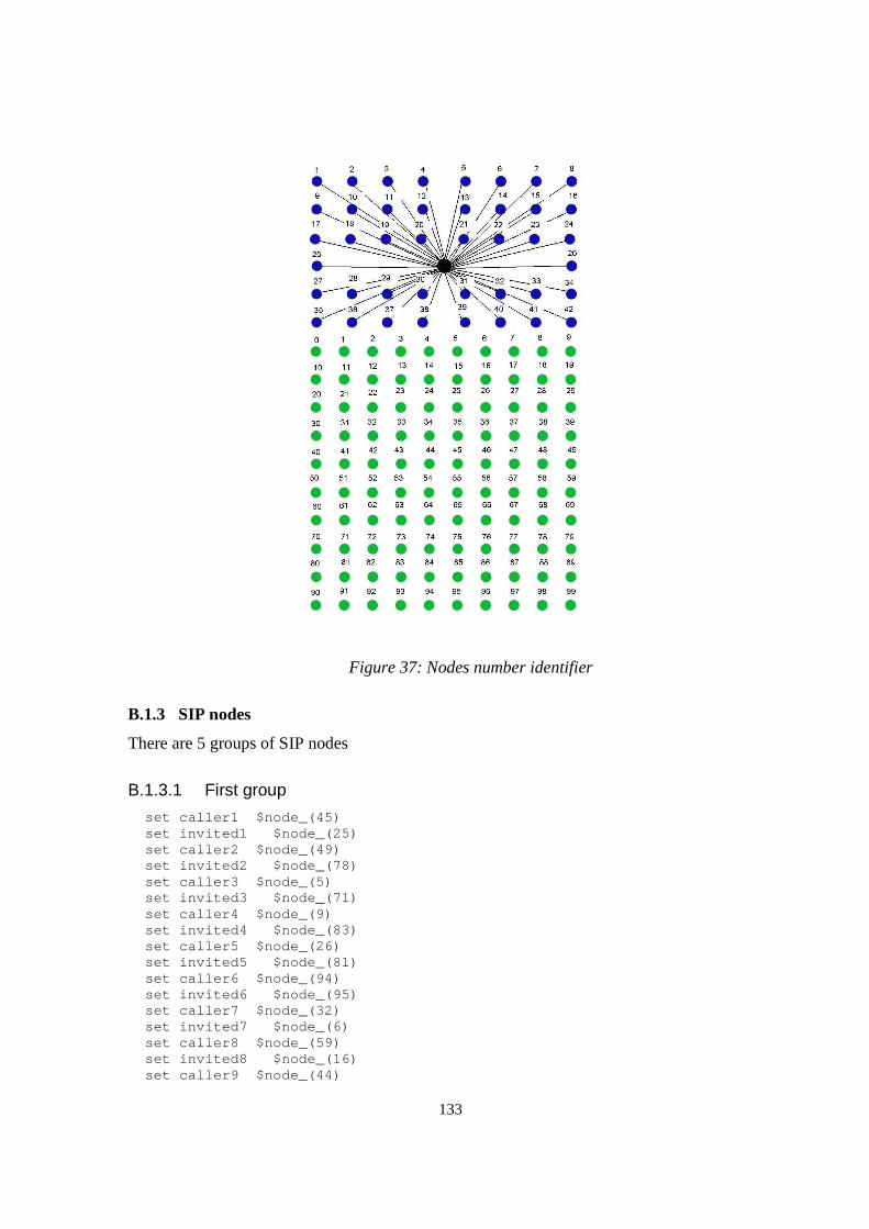
133
Figure 37: Nodes number identifier
B.1.3 SIP nodes
There are 5 groups of SIP nodes
B.1.3.1 First group
set caller1 $node_(45) set invited1 $node_(25) set caller2 $node_(49) set invited2 $node_(78) set caller3 $node_(5) set invited3 $node_(71) set caller4 $node_(9) set invited4 $node_(83) set caller5 $node_(26) set invited5 $node_(81) set caller6 $node_(94) set invited6 $node_(95) set caller7 $node_(32) set invited7 $node_(6) set caller8 $node_(59) set invited8 $node_(16) set caller9 $node_(44)
134
set invited9 $node_(80) set caller10 $node_(10) set invited10 $node_(34) set caller11 $node_(65) set invited11 $node_(55) set caller12 $node_(53) set invited12 $node_(69) set caller13 $node_(11) set invited13 $node_(24) set caller14 $node_(82) set invited14 $node_(38) set caller15 $node_(39) set invited15 $node_(8) set caller16 $node_(37) set invited16 $node_(1) set caller17 $node_(19) set invited17 $node_(3) set caller18 $node_(64) set invited18 $node_(0) set caller19 $node_(47) set invited19 $node_(43) set caller20 $node_(30) set invited20 $node_(20)
B.1.3.2 Second group
set caller1 $node_(89) set invited1 $node_(16) set caller2 $node_(30) set invited2 $node_(51) set caller3 $node_(75) set invited3 $node_(57) set caller4 $node_(23) set invited4 $node_(19) set caller5 $node_(56) set invited5 $node_(62) set caller6 $node_(92) set invited6 $node_(40) set caller7 $node_(31) set invited7 $node_(98) set caller8 $node_(38) set invited8 $node_(20) set caller9 $node_(34) set invited9 $node_(44) set caller10 $node_(68) set invited10 $node_(87) set caller11 $node_(93) set invited11 $node_(99) set caller12 $node_(25) set invited12 $node_(86) set caller13 $node_(90) set invited13 $node_(59) set caller14 $node_(33) set invited14 $node_(96) set caller15 $node_(79) set invited15 $node_(88)
135
set caller16 $node_(67) set invited16 $node_(50) set caller17 $node_(81) set invited17 $node_(24) set caller18 $node_(69) set invited18 $node_(42) set caller19 $node_(0) set invited19 $node_(52) set caller20 $node_(8) set invited20 $node_(70)
B.1.3.3 Third group
set caller1 $node_(48) set invited1 $node_(67) set caller2 $node_(50) set invited2 $node_(53) set caller3 $node_(35) set invited3 $node_(14) set caller4 $node_(19) set invited4 $node_(36) set caller5 $node_(0) set invited5 $node_(1) set caller6 $node_(26) set invited6 $node_(17) set caller7 $node_(55) set invited7 $node_(39) set caller8 $node_(9) set invited8 $node_(28) set caller9 $node_(88) set invited9 $node_(95) set caller10 $node_(11) set invited10 $node_(20) set caller11 $node_(64) set invited11 $node_(40) set caller12 $node_(51) set invited12 $node_(6) set caller13 $node_(61) set invited13 $node_(86) set caller14 $node_(49) set invited14 $node_(5) set caller15 $node_(68) set invited15 $node_(32) set caller16 $node_(25) set invited16 $node_(97) set caller17 $node_(58) set invited17 $node_(70) set caller18 $node_(12) set invited18 $node_(13) set caller19 $node_(92) set invited19 $node_(38) set caller20 $node_(33) set invited20 $node_(16)
136
B.1.3.4 Forth group
set caller1 $node_(37) set invited1 $node_(25) set caller2 $node_(4) set invited2 $node_(18) set caller3 $node_(68) set invited3 $node_(85) set caller4 $node_(69) set invited4 $node_(33) set caller5 $node_(78) set invited5 $node_(76) set caller6 $node_(79) set invited6 $node_(62) set caller7 $node_(73) set invited7 $node_(1) set caller8 $node_(9) set invited8 $node_(36) set caller9 $node_(88) set invited9 $node_(55) set caller10 $node_(87) set invited10 $node_(15) set caller11 $node_(44) set invited11 $node_(8) set caller12 $node_(57) set invited12 $node_(39) set caller13 $node_(26) set invited13 $node_(86) set caller14 $node_(12) set invited14 $node_(30) set caller15 $node_(65) set invited15 $node_(91) set caller16 $node_(98) set invited16 $node_(74) set caller17 $node_(96) set invited17 $node_(90) set caller18 $node_(28) set invited18 $node_(34) set caller19 $node_(56) set invited19 $node_(95) set caller20 $node_(71) set invited20 $node_(6)
B.1.3.5 Fifth group
set caller1 $node_(61) set invited1 $node_(13) set caller2 $node_(37) set invited2 $node_(2) set caller3 $node_(28) set invited3 $node_(82) set caller4 $node_(46) set invited4 $node_(68) set caller5 $node_(29) set invited5 $node_(8) set caller6 $node_(33) set invited6 $node_(30) set caller7 $node_(76)
137
set invited7 $node_(51) set caller8 $node_(38) set invited8 $node_(12) set caller9 $node_(25) set invited9 $node_(35) set caller10 $node_(7) set invited10 $node_(64) set caller11 $node_(40) set invited11 $node_(10) set caller12 $node_(66) set invited12 $node_(39) set caller13 $node_(75) set invited13 $node_(17) set caller14 $node_(43) set invited14 $node_(4) set caller15 $node_(56) set invited15 $node_(88) set caller16 $node_(55) set invited16 $node_(14) set caller17 $node_(50) set invited17 $node_(90) set caller18 $node_(71) set invited18 $node_(97) set caller19 $node_(89) set invited19 $node_(69) set caller20 $node_(93) set invited20 $node_(79)
B.1.4 Exponential nodes
B.1.4.1 Exponential nodes for 2 hops
set sender(0) $node_(1) set sender(1) $node_(7) set sender(2) $node_(69) set sender(3) $node_(63) set sender(4) $node_(31) set sender(5) $node_(25) set sender(6) $node_(65) set sender(7) $node_(70) set sender(8) $node_(11) set sender(9) $node_(45) set sender(10) $node_(76) set sender(11) $node_(60) set sender(12) $node_(43) set sender(13) $node_(14) set sender(14) $node_(57) set sender(15) $node_(82) set sender(16) $node_(20) set sender(17) $node_(34) set sender(18) $node_(58) set sender(19) $node_(83) set sender(20) $node_(32) set sender(21) $node_(38) set sender(22) $node_(74)
138
set sender(23) $node_(51) set sender(24) $node_(21) set sender(25) $node_(35) set sender(26) $node_(56) set sender(27) $node_(87) set sender(28) $node_(81) set sender(29) $node_(52) set sender(30) $node_(3) set sender(31) $node_(46) set receiver(0) $node_(10) set receiver(1) $node_(18) set receiver(2) $node_(78) set receiver(3) $W(3) set receiver(4) $node_(42) set receiver(5) $node_(36) set receiver(6) $W(4) set receiver(7) $node_(90) set receiver(8) $node_(13) set receiver(9) $W(5) set receiver(10) $node_(96) set receiver(11) $node_(80) set receiver(12) $W(6) set receiver(13) $node_(16) set receiver(14) $node_(68) set receiver(15) $node_(84) set receiver(16) $node_(40) set receiver(17) $W(7) set receiver(18) $node_(67) set receiver(19) $node_(94) set receiver(20) $node_(41) set receiver(21) $node_(49) set receiver(22) $W(8) set receiver(23) $node_(71) set receiver(24) $node_(30) set receiver(25) $node_(26) set receiver(26) $W(9) set receiver(27) $node_(89) set receiver(28) $node_(92) set receiver(29) $W(10) set receiver(30) $node_(5) set receiver(31) $node_(48)
B.1.4.2 Exponential nodes for 3 hops
set sender(0) $node_(1) set sender(1) $node_(8) set sender(2) $node_(79) set sender(3) $node_(51) set sender(4) $node_(2) set sender(5) $node_(9) set sender(6) $node_(57) set sender(7) $node_(60) set sender(8) $node_(10) set sender(9) $node_(6) set sender(10) $node_(66)
139
set sender(11) $node_(74) set sender(12) $node_(42) set sender(13) $node_(7) set sender(14) $node_(89) set sender(15) $node_(70) set sender(16) $node_(12) set sender(17) $node_(35) set sender(18) $node_(88) set sender(19) $node_(61) set sender(20) $node_(32) set sender(21) $node_(16) set sender(22) $node_(75) set sender(23) $node_(80) set sender(24) $node_(11) set sender(25) $node_(46) set sender(26) $node_(94) set sender(27) $node_(62) set sender(28) $node_(30) set sender(29) $node_(37) set sender(30) $node_(48) set sender(31) $node_(50) set receiver(0) $node_(4) set receiver(1) $node_(29) set receiver(2) $node_(98) set receiver(3) $W(3) set receiver(4) $node_(14) set receiver(5) $node_(17) set receiver(6) $W(4) set receiver(7) $node_(52) set receiver(8) $node_(40) set receiver(9) $node_(36) set receiver(10) $node_(96) set receiver(11) $W(5) set receiver(12) $W(6) set receiver(13) $node_(19) set receiver(14) $node_(97) set receiver(15) $node_(91) set receiver(16) $node_(0) set receiver(17) $W(7) set receiver(18) $node_(69) set receiver(19) $node_(64) set receiver(20) $node_(20) set receiver(21) $node_(28) set receiver(22) $W(8) set receiver(23) $node_(92) set receiver(24) $node_(41) set receiver(25) $W(9) set receiver(26) $node_(86) set receiver(27) $W(10) set receiver(28) $node_(33) set receiver(29) $node_(49) set receiver(30) $node_(78) set receiver(31) $node_(71)
140
B.1.4.3 Exponential nodes for 4 hops
set sender(0) $node_(3) set sender(1) $node_(18) set sender(2) $node_(78) set sender(3) $node_(83) set sender(4) $node_(20) set sender(5) $node_(19) set sender(6) $node_(76) set sender(7) $node_(61) set sender(8) $node_(1) set sender(9) $node_(25) set sender(10) $node_(68) set sender(11) $node_(50) set sender(12) $node_(32) set sender(13) $node_(28) set sender(14) $node_(66) set sender(15) $node_(71) set sender(16) $node_(11) set sender(17) $node_(16) set sender(18) $node_(95) set sender(19) $node_(94) set sender(20) $node_(12) set sender(21) $node_(17) set sender(22) $node_(85) set sender(23) $node_(80) set sender(24) $node_(14) set sender(25) $node_(36) set sender(26) $node_(59) set sender(27) $node_(60) set sender(28) $node_(52) set sender(29) $node_(26) set sender(30) $node_(69) set sender(31) $node_(62) set receiver(0) $node_(10) set receiver(1) $node_(39) set receiver(2) $node_(96) set receiver(3) $node_(3) set receiver(4) $node_(2) set receiver(5) $node_(37) set receiver(6) $node_(4) set receiver(7) $node_(92) set receiver(8) $node_(23) set receiver(9) $node_(5) set receiver(10) $node_(86) set receiver(11) $node_(81) set receiver(12) $node_(6) set receiver(13) $node_(6) set receiver(14) $node_(97) set receiver(15) $node_(75) set receiver(16) $node_(4) set receiver(17) $node_(29) set receiver(18) $node_(99) set receiver(19) $node_(7) set receiver(20) $node_(41) set receiver(21) $node_(57) set receiver(22) $node_(8)

141
set receiver(23) $node_(51) set receiver(24) $node_(9) set receiver(25) $node_(10) set receiver(26) $node_(88) set receiver(27) $node_(91) set receiver(28) $node_(21) set receiver(29) $node_(48) set receiver(30) $node_(98) set receiver(31) $node_(93)
B.1.4.4 Exponential nodes for 5 hops
set sender(0) $node_(5) set sender(1) $node_(16) set sender(2) $node_(98) set sender(3) $node_(71) set sender(4) $node_(0) set sender(5) $node_(8) set sender(6) $node_(59) set sender(7) $node_(50) set sender(8) $node_(14) set sender(9) $node_(26) set sender(10) $node_(56) set sender(11) $node_(63) set sender(12) $node_(13) set sender(13) $node_(7) set sender(14) $node_(58) set sender(15) $node_(74) set sender(16) $node_(21) set sender(17) $node_(35) set sender(18) $node_(55) set sender(19) $node_(70) set sender(20) $node_(1) set sender(21) $node_(19) set sender(22) $node_(68) set sender(23) $node_(93) set sender(24) $node_(10) set sender(25) $node_(17) set sender(26) $node_(88) set sender(27) $node_(80) set sender(28) $node_(31) set sender(29) $node_(37) set sender(30) $node_(65) set sender(31) $node_(84) set receiver(0) $node_(11) set receiver(1) $node_(39) set receiver(2) $node_(75) set receiver(3) $W(3) set receiver(4) $node_(41) set receiver(5) $node_(36) set receiver(6) $W(4) set receiver(7) $node_(33) set receiver(8) $node_(20) set receiver(9) $W(5) set receiver(10) $node_(79) set receiver(11) $node_(91)
142
set receiver(12) $W(6) set receiver(13) $node_(48) set receiver(14) $node_(86) set receiver(15) $node_(51) set receiver(16) $node_(44) set receiver(17) $node_(18) set receiver(18) $node_(96) set receiver(19) $node_(42) set receiver(20) $node_(24) set receiver(21) $node_(47) set receiver(22) $W(7) set receiver(23) $W(8) set receiver(24) $node_(15) set receiver(25) $node_(49) set receiver(26) $node_(94) set receiver(27) $node_(52) set receiver(28) $W(9) set receiver(29) $W(10) set receiver(30) $node_(97) set receiver(31) $node_(61)
B.1.4.5 Exponential nodes for 6 hops
set sender(0) $node_(5) set sender(1) $node_(14) set sender(2) $node_(84) set sender(3) $node_(70) set sender(4) $node_(3) set sender(5) $node_(7) set sender(6) $node_(87) set sender(7) $node_(91) set sender(8) $node_(1) set sender(9) $node_(16) set sender(10) $node_(57) set sender(11) $node_(75) set sender(12) $node_(21) set sender(13) $node_(24) set sender(14) $node_(35) set sender(15) $node_(32) set sender(16) $node_(38) set sender(17) $node_(92) set sender(18) $node_(2) set sender(19) $node_(97) set sender(20) $node_(50) set sender(21) $node_(4) set sender(22) $node_(61) set sender(23) $node_(64) set sender(24) $node_(12) set sender(25) $node_(69) set sender(26) $node_(56) set sender(27) $node_(33) set sender(28) $node_(43) set sender(29) $node_(93) set sender(30) $node_(95) set sender(31) $node_(25)
143
set receiver(0) $node_(10) set receiver(1) $node_(29) set receiver(2) $node_(79) set receiver(3) $W(3) set receiver(4) $node_(40) set receiver(5) $node_(58) set receiver(6) $W(4) set receiver(7) $node_(42) set receiver(8) $node_(52) set receiver(9) $W(5) set receiver(10) $node_(99) set receiver(11) $node_(80) set receiver(12) $W(6) set receiver(13) $node_(66) set receiver(14) $node_(86) set receiver(15) $node_(46) set receiver(16) $W(7) set receiver(17) $W(8) set receiver(18) $node_(44) set receiver(19) $node_(59) set receiver(20) $node_(34) set receiver(21) $node_(19) set receiver(22) $node_(94) set receiver(23) $node_(88) set receiver(24) $W(9) set receiver(25) $W(10) set receiver(26) $node_(83) set receiver(27) $node_(0) set receiver(28) $node_(37) set receiver(29) $node_(51) set receiver(30) $node_(68) set receiver(31) $node_(9)
B.1.4.6 Exponential nodes for 7 hops
set sender(0) $node_(5) set sender(1) $node_(4) set sender(2) $node_(58) set sender(3) $node_(91) set sender(4) $node_(12) set sender(5) $node_(33) set sender(6) $node_(88) set sender(7) $node_(50) set sender(8) $node_(0) set sender(9) $node_(28) set sender(10) $node_(86) set sender(11) $node_(60) set sender(12) $node_(11) set sender(13) $node_(25) set sender(14) $node_(64) set sender(15) $node_(44) set sender(16) $node_(20) set sender(17) $node_(79) set sender(18) $node_(61) set sender(19) $node_(35) set sender(20) $node_(32) set sender(21) $node_(21) set sender(22) $node_(41)

144
set sender(23) $node_(40) set sender(24) $node_(80) set sender(25) $node_(6) set sender(26) $node_(13) set sender(27) $node_(19) set sender(28) $node_(42) set sender(29) $node_(93) set sender(30) $node_(96) set sender(31) $node_(56) set receiver(0) $node_(30) set receiver(1) $node_(47) set receiver(2) $node_(95) set receiver(3) $W(3) set receiver(4) $node_(55) set receiver(5) $node_(18) set receiver(6) $W(4) set receiver(7) $node_(84) set receiver(8) $node_(52) set receiver(9) $W(5) set receiver(10) $node_(38) set receiver(11) $node_(94) set receiver(12) $W(6) set receiver(13) $node_(59) set receiver(14) $node_(98) set receiver(15) $node_(70) set receiver(16) $W(7) set receiver(17) $W(8) set receiver(18) $node_(46) set receiver(19) $node_(69) set receiver(20) $node_(74) set receiver(21) $node_(66) set receiver(22) $node_(26) set receiver(23) $node_(92) set receiver(24) $W(9) set receiver(25) $W(10) set receiver(26) $node_(65) set receiver(27) $node_(45) set receiver(28) $node_(76) set receiver(29) $node_(34) set receiver(30) $node_(48) set receiver(31) $node_(71)
145
C Post-tracing details
C.1 Post-tracing code files
C.1.1 Perl script to extract the exponential data and each SIP setup delay from
each simulation
This file calculates the jitter, average and percentile of exponential end to end delay.
# type: perl networkProductivity_v1.0.pl <trace fil e> > output file $infile=$ARGV[0]; open(trFile,$ARGV[0]) || die "we can not open the t race file $ARGV[0]\n"; while (<trFile>) { @values = split; $title= $values[0]; if ($title eq "parameters:") { print ("\n+++++++++++++++++++++++++++++++++++++++++++++++ ++++++++++++++++++++++\n"); print ("Simulation $values[2] gateways $values[3] h ops $values[4] exp_traffic flows $values[1] repetition \n"); print ("+++++++++++++++++++++++++++++++++++++++++++++++++ ++++++++++++++++++++\n"); # informative headers for CMUTracefile $number_gateways = $values[2]; $number_hops = $values[3]; $number_flows = $values [4]; } #-------------------------------------------------- ---------- #-------------------- WIRED TRACE FORMAT - ------- #-------------------------------------------------- ---------- if ($#values == 11) {
$event = $values[0]; $time = $values[1]; $from = $values [2]; $to = $values[3]; $pkt_type = $values[4]; $pkt_size = $values[5]; $source = $values[8]; $destiny = $values[9]; $pkt_id = $values[11];
#-------------------------------------------------- ---------- #-------------------- WIRED with EXP ----- --- #this part is to analyse the packet delay if ($pkt_type eq "exp") { if ($event eq "+") {
146
if ($state[$pkt_id] ne "sent") { if ($source =~ /0.0.$from/){ $start_time[$pkt_id] = $time; $state[$pkt_id]="sent"; $total_sent++; } } } if ($event eq "r") { if ($destiny =~ /0.0.$to/) { if ($state_end[$pkt_id] ne "received") { $end_time[$pkt_id] = $time; $packet_duration = $end_time[$pkt_id] - $start_time[$pkt_id]; $duration[$num_packets]=$packet_duration; $total_time = $total_time + $packet_duration; $num_packets++; $total_time_for_jitter = $total_time_for_jitter + $packet_duration; $quad = $quad + ($packet_duration*$packet_duration); $receives_delay_for _jitter++; $total_recv++; #print ("pakete recibido $pkt_id en tiempo $end_time[$pkt_id] y enviado en $start_time[$pkt_id ] con delay $packet_duration"); $state_end[$pkt_id]="received"; } } } } } #-------------------------------------------------- ---------- #-------------------- WIRELESS TRACE FORMAT -------- #-------------------------------------------------- ---------- if ($#values == 19) { $event = $values[0]; $time = $values[1]; $node = $values[2]; $trace_name = $values[3]; $reason = $values[4]; $pkt_id = $values[5]; $pkt_type = $values[6]; $pkt_size = $values[7]; $time_to_send = $values[8]; $MAC_dst = $values[9]; $MAC_src = $values[10]; $type = $values[11]; $flags = $values[12]; $IP_src = $values[13]; $IP_dst = $values[14]; $seq_num = $values[17]; $num_fwd = $values[18]; $optimal_fwd = $values[19]; #-------------------------------------------------- ----------
147
#-------------------- WIRELESS with EXP -- ------ #this part is to analyse the packet delay if ($pkt_type eq "exp") { if ($event eq "s") { if ($state[$pkt_id] ne "sent") { $start_time[$pkt_id] = $time; $state[$pkt_id]="sent"; $total_sent++; } } if ($event eq "r") { if ($state_end[$pkt_id] ne "received") { $end_time [$pkt_id] = $time; $state_end[$pkt_id]="received"; $packet_duration = $end_time[$pkt_id] - $start_time[$pkt_id]; $duration[$num_packets]=$packet_duration; $total_time = $total_time + $packet_duration; $num_packets++; $total_time_for_jitter = $total_time_for_jitter + $packet_duration; $quad = $quad + ($packet_duration*$packet_duration); $receives_delay_for_jitter+ +; $total_recv++; } } } } #-------------------------------------------------- ------- #------------wireless for sip calls --------------- ------- #-------------------------------------------------- ------- if ($#values==19) { $event = $values[0]; $time = $values[1]; $node = $values[2]; $trace_name = $values[3]; $reason = $values[4]; $pkt_id = $values[5]; $pkt_type = $values[6]; $pkt_size = $values[7]; $time_to_send = $values[8]; $MAC_dst = $values[9]; $MAC_src = $values[10]; $type = $values[11]; $flags = $values[12]; $IP_src = $values[13]; $IP_dst = $values[14]; $TTL = $values[15]; $next_hop = $values[16]; $seq_num = $values[17]; $num_fwd = $values[18]; $optimal_fwd = $values[19]; #this part is to analyce the SIP call delay set up if ($event eq "s") { if ($values[6] eq "SIP_INVITE") { if ($values[7] eq "800") {
148
$concat_sent=$node.$seq_num; if ($invitado{$concat_sent} ne "1") { $start_SIP_call{$concat_sent}=$time; $invitado{$concat_sent}="1"; } } } } if ($event eq "r") { if ($pkt_type eq "SIP_200") { if ($pkt_size eq "530") { $concat_rec = $node.$seq_num; if ($accepted{$concat_rec} ne "1"){ $accepted{$concat_rec}="1"; $accepted_SIP_call{$concat_rec}=$time; $sip_call_delay[$sip_aceptados]=$accepted_SIP_call {$concat_rec}-$start_SIP_call{$concat_rec}; $total_sip_call_delay=$total_sip_call_delay + $sip_call_delay[$sip_aceptados]; $sip_aceptados++; } } } } #to get the number of hops if ($event eq "r") { if ($pkt_type eq "SIP_100") { if ($pkt_size eq "230") { if ($already{$node} ne "yes"){ $already{$node}="yes"; #print ("node $node tiempo $time recibio el 100_ok\n"); $total_hops= $total_hops + $num_fwd; $num_calculated_hops++; } } } if ($pkt_type eq "SIP_INVITE") { if ($pkt_size eq "780") { if ($already{$node} ne "yes"){ $already{$node}="yes"; #print ("nodo : $node tiempo $time rebibio invitacion\n "); $total_hops= $total_hops + $num_fwd; $num_calculated_hops++; } } } } } }
149
#este braket es del principio close (trFile); #################################### ##########FOR EXP TRAFFIC########### #################################### #this is the average delay if ($num_packets != 0) {$avg_delay = $total_time/$n um_packets; @durationsort=sort {$a<=>$b}(@duration); #compute 95 percenti #for the exp packets for ($i=0;$i<$num_packets;$i++) {
$variation_temp = $durationsort[$i] - $avg_delay; $variation_abs=abs($variation_temp); $square_variation= $variation_temp * $variation_tem p; $square_total = $square_total + $square_variation; }
$variance = $square_total / $num_packets; $square_root_variance = sqrt ($variance); $square_root_num_packets = sqrt ($num_packets); $standar_error = $square_root_variance / $square_ro ot_num_packets; $percentil1 = $avg_delay-(1.96 * $standar_error ); $percentil2 = $avg_delay+(1.96 * $standar_error ); #------------------- #------------------- if ($receives_delay_for_jitter != 0 ) { $delay_variance = $quad / $receives_delay_for_jitte r; $jitter_delay = $delay_variance - ($total_delay*$to tal_delay); } #################################### #################################### print "#######---------------------------########\n "; print "#######------exp traffic----------########\n "; print "#######---------------------------########\n "; if ($num_packets != 0) {$total_delay = $total_time/ $num_packets;}
print "exp: packets_sent: $total_sent\n"; print "exp: packets_received: $total_recv\n"; $temp1 = $total_sent - $total_recv; $temp2 = $temp1 / $total_sent; print "exp: packet_lost_probability: $temp2\n"; print "exp: avg_delay: $avg_delay\n"; print "exp: Max_delay: $durationsort[$num_packets-1 ] \n"; print "exp: Min_delay: $durationsort[0]\n"; $jitter = sqrt ($jitter_delay); print "exp: Jitter_delay: $jitter\n"; print "exp: 95_percentil_range: [ $percentil1 , $pe rcentil2 ]\n"; print "\n";
} @sip_call_delay_sort=sort {$a<=>$b}(@sip_call_delay ); print "#######---------------------------########\n "; print "#######---sip call invitations----########\n "; print "#######---------------------------########\n ";
150
print "sip: total_hops: $total_hops\n"; print "sip: counted_hops: $num_calculated_hops\n"; print "number accepted sip call: $sip_aceptados\n"; $temp = $num_calculated_hops / 2; $avg_hops = $total_hops / $temp; print "sip: avg_hops: $avg_hops\n"; for ($x=0;$x<$sip_aceptados;$x++) {
print "sip: sip_time: $sip_call_delay_sort[$x]\n"; }
C.1.2 Perl script to make the average of Exponential and SIP values already
extracted with Perl script C.1.1.
This file takes the Exponential and SIP values of each simulation to make a new file with
new data of 5 repetitions of one simulation. It calculates the jitter, average and percentile
of SIP setup delays. It calculates the call block probability as well.
This creates two files with the SIP setup delay by times in an appropriated format to
plot the graphs with Gnuplot.
# type: perl averag.....pl <trace file> > outp ut file sub average { local($n, $somma, $media); foreach $n (@_) { $somma += $n; } $media = $somma/($#_+1); return ($media); } sub jitter { local($n, $somma, $media,$quad,$variance,$sqr_avg,$ sqr_jitter); $n = 0; $somma = 0; $media = 0; $quad = 0; $variance = 0; $sqr_avg = 0; $sqr_jitter = 0; $computed_jitter = 0; foreach $n (@_) { $somma += $n; } $media = $somma/($#_+1); foreach $n (@_) { $quad += $n * $n; } $variance = $quad /($#_+1); $sqr_avg = $media * $media; $sqr_jitter = $variance - $sqr_avg; $computed_jitter = sqrt($sqr_jitter); return ($computed_jitter); }
151
sub percentil { local($n, $somma, $media); $n = 0; $somma = 0; $media = 0; $variation_temp = 0; $square_variation = 0; $square_total = 0; $variance = 0; $square_root_variance = 0; $square_root_num_packets = 0; $standar_error = 0; foreach $n (@_) { $somma += $n; } $media = $somma/($#_+1); foreach $n (@_) { $variation_temp = $n - $media; $square_variation= $variation_temp * $variation_tem p; $square_total = $square_total + $square_variation; } $variance = $square_total / ($#_+1); $square_root_variance = sqrt ($variance); $square_root_num_packets = sqrt ($#_+1); $standar_error = $square_root_variance / $square_ro ot_num_packets; $percentil1 = $media - (1.96 * $standar_error ); $percentil2 = $media + (1.96 * $standar_error ); return ("[$percentil1,$percentil2]"); } $infile=$ARGV[0]; $number_sip = 0; $number_sip_within_2 = 0; $number_sip_within_5 = 0; $number_sip_within_10 = 0; $number_repetitions = 0; open(trFile,$ARGV[0]) || die "we can not open the t race file $ARGV[0]\n"; while (<trFile>) { @values = split; # working with exp results if ($values[0] eq "Simulation") { $number_repetitio ns++; } $title= $values[0]; if ($already_title != 1) { if ($title eq "Simulation") { $already_title = 1; print ("################******************######### ##########\n"); print ("Simulation $values[1] gateways $values[3] h ops $values[5] flows \n"); print ("#################****************########## ######\n"); $number_flows = $values[5]; $gateways=$values[1]; $hops=$values[3]; }
152
} if ($values[0] eq "exp:") { if ($values[1] eq "packets_sent:") { $total_packets_sent += $values[2]; $cont_packets_sent += 1; } if ($values[1] eq "packets_received:") { $total_packets_recev += $values[2]; $cont_packets_recev += 1; } if ($values[1] eq "avg_delay:") { $total_delay += $values[2]; $cont_delay += 1; } if ($values[1] eq "Max_delay:") { if ($Max_delay < $values[2]) {$Max_delay = $value s[2];} } if ($values[1] eq "Min_delay:") { if ($Min_delay < $values[2]) {$Min_delay = $value s[2];} } if ($values[1] eq "Jitter_delay:") { $total_jitter += $values[2]; $cont_jitter += 1; } if ($values[1] eq "packet_lost_probability:") { $total_p_l_p += $values[2]; $cont_p_l_p += 1; } if ($values[1] eq "95_percentil_range:") { $min_95perc += $values[3]; $max_95perc += $values[5]; $cont_95perc +=1; } } # working with sip results if ($values[0] eq "sip:") { if ($values[1] eq "sip_time:") { $sip_times[$number_sip] = $values[2]; $number_sip += 1; if ($values[2] < 2) { $sip_times_within_2[$number_sip_within_2]=$value s[2]; $number_sip_within_2++; } if ($values[2] < 5) { $sip_times_within_5[$number_sip_within_5]=$value s[2]; $number_sip_within_5++; } if ($values[2] < 10) { $sip_times_within_10[$number_sip_within_10]=$value s[2]; $number_sip_within_10++; } } if ($values[1] eq "avg_hops:") {

153
$total_hops += $values[2]; $cont_hops += 1; } } } close (trFile); # compute for exp results if ($total_packets_recev != 0 ) { $total_sent = $total_packets_sent / $cont_packets_s ent; $total_recv = $total_packets_recev / $cont_packets_ recev; $packet_lost_prob = $total_p_l_p / $cont_p_l_p; $avg_delay = $total_delay / $cont_delay; $jitter = $total_jitter / $cont_jitter; $exp_percentil1 = $min_95perc / $cont_95perc; $exp_percentil2 = $max_95perc / $cont_95perc; print "$number_flows flows #####\n"; print "$number_flows flows #######-------exp traffi c average 5 simulations----########\n"; print "$number_flows flows #####\n"; print "$number_flows flows exp: packets_sent: $tota l_sent\n"; print "$number_flows flows exp: packets_recibidos: $total_recv\n"; print "$number_flows flows exp: packets_lost_prob: $packet_lost_prob\n"; print "$number_flows flows exp: avg_delay: $avg_del ay\n"; print "$number_flows flows exp: Max_delay: $Max_del ay \n"; print "$number_flows flows exp: Min_delay: $Min_del ay\n"; print "$number_flows flows exp: Jitter_delay : $jit ter\n"; print "$number_flows flows exp: 95_percentil_range: [ $exp_percentil1 , $exp_percentil2 ]\n"; print "\n"; } if ($number_sip != 0 ) { @sip_times_sort=sort{$a<=>$b}(@sip_times); $avg_hops = $total_hops / $cont_hops; print "$number_flows flows #######----------------- ----------------------------########\n"; print "$number_flows flows #######------------ALL S IP CALL INVITATIONS---------########\n"; print "$number_flows flows #######----------------- ----------------------------########\n"; print ""; print "$number_flows flows sip: hops_avg: $avg_hops \n"; $possible = $number_repetitions * 20; $not_done = $possible - $number_sip; $block_p=$not_done/$possible; $sip_avg = &average(@sip_times_sort); print "$number_flows flows sip: sip_call_block_prob ability: $block_p \n"; print "$number_flows flows sip: avg_delay: ";print &average(@sip_times_sort); print "\n$number_flows flows sip: Max_delay: $sip_times_sort[$number_sip-1] \n"; print "$number_flows flows sip: Min_ delay: $sip_ti mes_sort[0]\n";
154
print "$number_flows flows sip: Jitter_delay : ";pr int &jitter(@sip_times_sort); print "\n$number_flows flows sip: 95_percentil_rang e: ";print &percentil(@sip_times_sort); print "\n"; foreach $n (@sip_times_sort) { $x = int($n); print ("\n $number_flows flows sip: sip_time s: $n $x "); $calls_per_second[$x]++; } $fileA="calls_per_seconds_.$gateways.gateways.$hops .hops.$number_flows.flows.dat"; $fileB="calls_until__second_.$gateways.gateways.$ho ps.hops.$number_flows.flows.dat"; open (A,">$fileA"); open (B,">$fileB"); print A "#calls_per_second simulation gateways:$values[1]hops:$values[3]flows:$number_flo ws"; print B "#calls_until_second simulation gateways: $ values[1]hops: $values[3] flows: $number_flows"; for ($i = 0; $i<=$x+1; $i++) { if (exists $calls_per_second[$i]){ print A ("\n$i\t$calls_per_second[$i]"); }else{ print A ("\n$i\t0"); } } for ($i = 0; $i<=$x+1; $i++) { $calls_until_second[$i]=$calls_per_second[$i]+$call s_until_second[$i-1]; print B ("\n$i\t$calls_until_second[$i]"); } close(A); close(B); print "\n"; my @calls_per_second = (); } if ($number_sip_within_10 != 0 ) { @sip_times_within_10_sort=sort{$a<=>$b}(@sip_times_ within_10); print "#######------------------------------------- --------########\n"; print "#######----------SIP CALL WITHIN 10 SECONDS- ---------########\n"; print "#######------------------------------------- --------########\n"; $possible10 = $number_repetitions * 20; $not_done10 = $possible10 - $number_sip_within_10; $block_p10=$not_done10/$possible10; print "$number_flows flows sip_valid_10: sip_valid_ call_probability: $block_p10\n"; print "$number_flows flows sip_valid_10: avg_delay: "; print &average(@sip_times_within_10_sort); print "\n$number_flows flows sip_valid_10: Max_dela y: $sip_times_within_10_sort[$number_sip_within_10-1] \n"; print "$number_flows flows sip_valid_10: Min_delay: $sip_times_within_10_sort[0]\n"; print "$number_flows flows sip_valid_10: Jitter_del ay : ";
155
print &jitter(@sip_times_within_10_sort); print "\n$number_flows flows sip_valid_10: 95_perce ntil_range: "; print &percentil(@sip_times_within_10_sort); print "\n"; } if ($number_sip_within_5 != 0 ) { @sip_times_within_5_sort=sort{$a<=>$b}(@sip_times_w ithin_5); print "#######------------------------------------- --------########\n"; print "#######----------SIP CALL WITHIN 5 SECONDS-- --------########\n"; print "#######------------------------------------- --------########\n"; $possible5 = $number_repetitions * 20; $not_done5 = $possible5 - $number_sip_within_5; $block_p5=$not_done5/$possible5; print "$number_flows flows sip_valid_5: sip_valid_c all_probability: $block_p5\n"; print "$number_flows flows sip_valid_5: avg_delay:" ; print &average(@sip_times_within_5_sort); print "\n$number_flows flows sip_valid_5: Max_delay : $sip_times_within_5_sort[$number_sip_within_5-1] \n "; print "$number_flows flows sip_valid_5: Min_delay: $sip_times_within_5_sort[0]\n"; print "$number_flows flows sip_valid_5: Jitter_dela y :"; print &jitter(@sip_times_within_5_sort); print "\n$number_flows flows sip_valid_5: 95_percen til_range:"; print &percentil(@sip_times_within_5_sort); print "\n"; } if ($number_sip_within_2 != 0 ) { @sip_times_within_2_sort=sort{$a<=>$b}(@sip_times_w ithin_2); print "#######------------------------------------- --------########\n"; print "#######----------SIP CALL WITHIN 2 SECONDS-- --------########\n"; print "#######------------------------------------- --------########\n"; $possible2 = $number_repetitions * 20; $not_done2 = $possible2 - $number_sip_within_2; $block_p2=$not_done2/$possible2; print "$number_flows flows sip_valid_2: sip_valid_c all_probability: $block_p2\n"; print "$number_flows flows sip_valid_2: avg_delay:" ;print &average(@sip_times_within_2_sort); print "\n$number_flows flows sip_valid_2: Max_delay : $sip_times_within_2_sort[$number_sip_within_2-1] \n "; print "$number_flows flows sip_valid_2: Min_delay: $sip_times_within_2_sort[0]\n"; print "$number_flows flows sip_valid_2: Jitter_dela y :"; print &jitter(@sip_times_within_2_sort); print "\n$number_flows flows sip_valid_2: 95_percen til_range:";print &percentil(@sip_times_within_2_sort); print "\n"; }
C.1.3 Perl script to count the number of SIP hops
This file count the number of SIP hops when the session get initiated.
$infile=$ARGV[0];

156
$total_hops=0; $num_calculated_hops=0; open(trFile,$ARGV[0]) || die "we can not open the t race file $ARGV[0]\n"; while (<trFile>) { @values = split; $title= $values[0]; if ($title eq "parameters:") { print ("\n+++++++++++++++++++++++++++++++++++++++++++++++ ++++++++++++++++++++++\n"); print ("Simulation $values[2] gateways $values[3] h ops $values[4] exp_traffic flows $values[1] repetition \n"); print ("+++++++++++++++++++++++++++++++++++++++++++++++++ ++++++++++++++++++++\n"); # informative headers for CMUTracefile $number_gateways = $values[2]; $number_hops = $values[3]; $number_flows = $values [4]; } #------------wireless for sip calls --------------- ------- if ($#values==19) { $event = $values[0]; $time = $values[1]; $node = $values[2]; $trace_name = $values[3]; $reason = $values[4]; $pkt_id = $values[5]; $pkt_type = $values[6]; $pkt_size = $values[7]; $time_to_send = $values[8]; $MAC_dst = $values[9]; $MAC_src = $values[10]; $type = $values[11]; $flags = $values[12]; $IP_src = $values[13]; $IP_dst = $values[14]; $TTL = $values[15]; $next_hop = $values[16]; $seq_num = $values[17]; $num_fwd = $values[18]; $optimal_fwd = $values[19]; #to get the number of hops if ($event eq "r") { if ($pkt_type eq "SIP_200") { if ($pkt_size eq "530") { $total_hops= $total_hops + $num_fwd; $num_calculated_hops++; } }
157
} if ($pkt_type eq "SIP_ACK") { if ($pkt_size eq "280") { $total_hops= $total_hops + $num_fwd; $num_calculated_hops++; } } } } } } #este braket es del principio close (trFile); print "hp: $number_hops gt: $number_gateways fl: $n umber_flows total_hops: $total_hops number_calls: $num_calculat ed_hops\n");
C.1.4 Perl script to extract the exponential information of each exponential traffic
flow
This script is important because this calculate all the performance parameters for each
exponential traffic flow separately.
# type: perl network_by_exp <trace file> > out put file sub average { local($n, $somma, $media); foreach $n (@_) { $somma += $n; } $media = $somma/($#_+1); return ($media); } sub jitter { local($n, $somma, $media,$quad,$variance,$sqr_avg,$ sqr_jitter); $n = 0; $somma = 0; $media = 0; $quad = 0; $variance = 0; $sqr_avg = 0; $sqr_jitter = 0; $computed_jitter = 0; foreach $n (@_) { $somma += $n; } $media = $somma/($#_+1);
158
foreach $n (@_) { $quad += $n * $n; } $variance = $quad /($#_+1); $sqr_avg = $media * $media; $sqr_jitter = $variance - $sqr_avg; $computed_jitter = sqrt($sqr_jitter); return ($computed_jitter); } sub percentil { local($n, $somma, $media); $n = 0; $somma = 0; $media = 0; $variation_temp = 0; $square_variation = 0; $square_total = 0; $variance = 0; $square_root_variance = 0; $square_root_num_packets = 0; $standar_error = 0; foreach $n (@_) { $somma += $n; } $media = $somma/($#_+1); foreach $n (@_) { $variation_temp = $n - $media; $square_variation= $variation_temp * $variation_tem p; $square_total = $square_total + $square_variation; } $variance = $square_total / ($#_+1); $square_root_variance = sqrt ($variance); $square_root_num_packets = sqrt ($#_+1); $standar_error = $square_root_variance / $square_ro ot_num_packets; $percentil1 = $media - (1.96 * $standar_error ); $percentil2 = $media + (1.96 * $standar_error ); return ("$percentil1,$percentil2"); } $infile=$ARGV[0]; $flows_identified = 0; open(trFile,$ARGV[0]) || die "we can not open the t race file $ARGV[0]\n"; while (<trFile>) { @values = split; $title= $values[0]; if ($title eq "parameters:") { print ("\n+++++++++++++++++++++++++++++++++++++++++++++++ ++++++++++++++++++++++\n"); print ("Simulation $values[2] gateways $values[3] h ops $values[4] exp_traffic flows $values[1] repetition \n");
159
print ("+++++++++++++++++++++++++++++++++++++++++++++++++ ++++++++++++++++++++\n"); $number_flows = $values[4]; } #-------------------------------------------------- ---------- ###-------------------- WIRED TRACE FORMAT -------- ###------------------------------------------------ ------------ if ($#values == 11) { $event = $values[0]; $time = $values[1]; $from = $values [2]; $to = $values[3]; $pkt_type = $values[4]; $pkt_size = $values[5]; $source = $values[8]; $destiny = $values[9]; $pkt_id = $values[11]; #-------------------------------------------------- ---------- ##-------------------- WIRED with EXP ---- ---- # ##this part is to analyse the packet delay if ($pkt_type eq "exp") { if ($event eq "+") { if ($state[$pkt_id] ne "sent") { if ($source =~ /0.0.$from/){ $src = substr($source,0,leng th($source)-2); $dst = substr($destiny,0,len gth($destiny)-2); $concat_1 = $src.".".$dst; $concat_2 = $dst.".".$src; #print ("$concat_1............$concat_2\n" ); $flow_id = "xx"; for ($i=0;$i<$flows_identified;$i++) { if (($concat_1 eq $flow[$i]) or ($concat_2 eq $flow[$i])) { # print ("ver si son iguales en wired:conc at 1 :$concat_1......$flow[$i].....concat 2 ::::$concat_2.....$flow[$i]...\n"); $flow_id = $i; $iguales++; } } if ($flow_id eq "xx") { #print ("concat 1 :::$concat_1......$flow[$i].... .concat 2 :::::$concat_2.....$flow[$i]...\n"); # print ("no existe en wired.............$flows_i dentified\n"); $flow[$flows_identified] = $concat_1; $flow_id=$flow_identified; $flows_identified++; } $start_time[$pkt_id] = $time; $state[$pkt_id]="sent"; $total_sent[$flow_id]++;
160
} } } if ($event eq "r") { if ($destiny =~ /0.0.$to/) { if ($state_end[$pkt_id] ne "received") { #print ("esta es fuente y destino de $source.........$destiny \n"); $src = substr($source,0,length($source)-2); $dst = substr($destiny,0,length($destiny)-2); #print ("esta esl a fuente y destino despues de sustraer el numero de puerto $concat_1............$ concat_2 \n"); $concat_1 = $src.".".$dst; $concat_2 = $dst.".".$src; #print ("$concat_1............$concat_2\n"); $flow_id = "xx"; for ($i=0;$i<$flows_identified;$i++) { if (($concat_1 eq $flow[$i]) or ($concat_2 eq $flow[$i])) { $flow_id = $i; $iguales++; } } if ($flow_id eq "xx") { # print ("concat 1 :::$concat_1......$flow[$i].. ...concat 2 :::::$concat_2.....$flow[$i]...\n"); # print ("no existe en wired.............$flows_identified\n"); $flow[$flows_identified] = $concat _1; $flow_id=$flow_identified; $flows_identified++; } if ($state[$pkt_id] eq "sent") { $end_time[$pkt_id] = $time; $packet_duration = $end_time[$pkt_id] - $s tart_time[$pkt_id]; $duration[$flow_id][$total_recv[$flow_id]] =$packet_duration; $total_time[$flow_id] = $total_time[$flow_ id] + $packet_duration; $total_time_for_jitter[$flow_id] = $total_time_for_jitter[$flow_id] + $packet_duration ; $quad[$flow_id] = $quad[$flow_id] + ($packet_duration*$packet_duration); $receives_delay_for_jitter[$flow_id]++; $total_recv[$flow_id]++; #print ("pakete recibido $pkt_id en tiempo $end_time[$pkt_id] y enviado en $start_time[$pkt_id] con delay $packet _duration"); $state_end[$pkt_id]="received"; } } } } } } #-------------------- WIRELESS TRACE FORMAT -------- #-------------------------------------------------- ----------
161
if ($#values == 19) { $event = $values[0]; $time = $values[1]; $node = $values[2]; $trace_name = $values[3]; $reason = $values[4]; $pkt_id = $values[5]; $pkt_type = $values[6]; $pkt_size = $values[7]; $time_to_send = $values[8]; $MAC_dst = $values[9]; $MAC_src = $values[10]; $type = $values[11]; $flags = $values[12]; $IP_src = $values[13]; $IP_dst = $values[14]; $seq_num = $values[17]; $num_fwd = $values[18]; $optimal_fwd = $values[19]; #-------------------------------------------------- ---------- #-------------------- WIRELESS with EXP -- ------ if ( $pkt_type eq "exp" ) { @separada = split(/:/, $IP_src); @separada2=split (//,$separada[0]); $src = $separada[0]; if ($separada2[0] eq "["){ $src = substr($separada[0],1,length($separ ada[0])); } @separada = split(/:/, $IP_dst); @separada2=split (//,$separada[0]); $dst = $separada[0]; if ($separada2[0] eq "["){ $dst = substr($separada[0],1,length($separ ada[0])); } $concat_1 = $src.".".$dst; $concat_2 = $dst.".".$src; #print ("$concat_1............$concat_2\n"); $flow_id = "xx"; for ($i=0;$i<$number_flows;$i++) { if (($concat_1 eq $flow[$i]) or ($concat_2 eq $flow[$i])) { $flow_id = $i; $iguales++; } } if ($flow_id eq "xx") { #print ("no existe.............$flows_identified \n"); $flow[$flows_identified] = $concat_1; $flow_id=$flow_identified; $flows_identified++; }

162
#this part is to analyse the packet delay if ($pkt_type eq "exp") { if ($event eq "s") { if ($state[$pkt_id] ne "sent") { $start_time[$pkt_id] = $time; $state[$pkt_id]="sent"; $total_sent[$flow_id]++; } } if ($event eq "r") { if ($state_end[$pkt_id] ne "received") { if ($state[$pkt_id] eq "sent") { $end_time [$pkt_id] = $time; $state_end[$pkt_id]="received"; $packet_duration = $end_time[$pkt_id] - $start_time[$pkt_id]; $duration[$flow_id][$total_recv[$flow_id]]=$packet _duration; $total_time[$flow_id] = $total_time[$flow_id] + $packet_duration; $total_time_for_jitter[$flow_id] = $total_time_for_jitter[$flow_id] + $packet_duration ; $quad[$flow_id] = $quad[$flow_id] + ($packet_duration*$packet_duration); $receives_delay_for_jitter[$flow_id]++; $total_recv[$flow_id]++; } } } } } } } close (trFile); #################################### ##########FOR EXP TRAFFIC########### #################################### for ($i=0;$i<$flows_identified;$i++) { my @temp_matrix = (); for ($x=0;$x<$total_recv[$i];$x++) { $temp_matrix[$x] = $duration[$i][$x]; } @temp_matrix_sort=sort{$a<=>$b}(@temp_matrix); #print "#######---------------------------########\ n"; print "####### flow number $i : $flow[$i]#######\n "; #print "#######---------------------------########\ n"; #print ("exp: packets_received: $total_recv[$i] \n" ); #print ("exp: packets_sent: $total_sent[$i] \n"); $temp1 = $total_sent[$i] - $total_recv[$i]; $temp2 = $temp1 / $total_sent[$i]; print ("parties_flow: $flow[$i]\n"); print "hp: $values[3] gt: $values[2] fl: $values[4] plr: $temp2\t"; print ("avg_delay: ");print &average(@temp_matrix_s ort); print "\tMax_delay: $temp_matrix_sort[$total_recv[$ i]-1]\t";
163
print "Min_delay: $temp_matrix_sort[0]\t"; print "Jitter_delay :"; print &jitter(@temp_matrix_ sort); print "\t95_percent: ";print &percentil(@temp_matri x_sort); print ("\n"); }
C.1.5 Perl script to calculate the percentage of valid calls
This file extract the percentage of valid calls from the file which is generated with all
the exponential traffic flows performance parameters calculated in C.1.4
$infile=$ARGV[0]; my @valids = (); my @invalids = (); my @percent_valids = (); open(trFile,$ARGV[0]) || die "we can not open the t race file $ARGV[0]\n"; while (<trFile>) { @values = split; $first_word= $values[0]; if ($first_word eq "hp:") { $number_hops = $values[1]; $number_gateways = $values[3]; $number_flows = $values[5]; $plr = $values[7]; $avg_delay = $values[9]; if (($plr < 0.05) & ($avg_delay < 0.125)){ $valids[$number_hops][$number_gateways][$number_fl ows] = $valids[$number_hops][$number_gateways][$number_flo ws] + 1 ; } else { $invalids[$number_hops][$number_gateways][$number_ flows] = $invalids[$number_hops][$number_gateways][$number_f lows] + 1 ; } } } $gateway[0]=1; $gateway[1]=2; $gateway[2]=4; $flows[0]=4; $flows[1]=8; $flows[2]=12; $flows[3]=16; $flows[4]=24; $flows[5]=32; for ($x = 2; $x<8; $x++) { # este for es para los n umero de hops $fileA="exponential_valids.$x.hops.dat";

164
open (A,">$fileA"); for ($j = 0; $j<6; $j++) { # este for es para nume ro de flows for ($i = 0; $i<3; $i++) { # este para las gatewa ys $validas = $valids[$x][$gateway[$i]][$flows[$j]]; $invalidas = $invalids[$x][$gateway[$i]][$flows[$ j]]; $total =$validas+$invalidas; $result = $validas/$total; #print ("aki el total y validas $total $validas") ; $result = $result*100; #$total = $valids[$x][$gateway[$i]][$flows[$i]] + $invalids[$x][$gateway[$i]][$flows[$i]]; } print A ("\n"); } close (A); }
C.1.6 Perl script to create SIP user nodes randomly
This file chooses 40 nodes to be SIP user nodes. The first lines don’t allow the script
to choose the nodes that act as gateways.
$i=6; $randon[1]=22; $randon[2]=27; $randon[3]=72; $randon[4]=77; $randon[5]=54; while ($i <= 46) { $a=rand (100); $b= int($a); $state = "different"; #print("$state\n"); foreach $x (@randon) { if ($b eq $x) { # it is already choosen $state = "already"; } } if ($state ne "already"){ $randon[$i]=$b; # print ("the node number $i is $b\n"); $i++; }
165
} print("++++++++++++++++++++++++++"); print("+++ print all nodes +++"); print("++++++++++++++++++++++++++"); foreach $valid (@randon) { print(" $valid \n"); }
C.1.7 Perl script to extract the exponential packet loss rate classified in intra and
outgoing traffic flows
$infile=$ARGV[0]; my @valids = (); my @invalids = (); my @percent_valids = (); open(trFile,$ARGV[0]) || die "we can not open the t race file $ARGV[0]\n"; while (<trFile>) { @values = split; $first_word= $values[0]; if ($first_word eq "parties_flow:") { $parties = $values[1]; if ($parties =~ /0.0./) { $state = "out"; }else{ $state = "in"; } } if ($first_word eq "hp:") { $number_hops = $values[1]; $number_gateways = $values[3]; $number_flows = $values[5]; $plr = $values[7]; $avg_delay = $values[9]; if ($state eq "out"){ $plr_out[$number_hops][$number_gateways][$number_f lows] = $plr_out[$number_hops][$number_gateways][$number_fl ows] + $plr ; $count_plr_out[$number_hops][$number_gateways][$nu mber_flows] = $count_plr_out[$number_hops][$number_gateways][$num ber_flows]+1; } if ($state eq "in"){ $plr_in[$number_hops][$number_gateways][$number_fl ows] = $plr_in[$number_hops][$number_gateways][$number_flo ws] + $plr ; $count_plr_in[$number_hops][$number_gateways][$num ber_flows] = $count_plr_in[$number_hops][$number_gateways][$numb er_flows]+1; } }

166
} $gateway[0]=1; $gateway[1]=2; $gateway[2]=4; $flows[0]=4; $flows[1]=8; $flows[2]=12; $flows[3]=16; $flows[4]=24; $flows[5]=32; $fileA="plr_out.dat"; open (A,">$fileA"); for ($x = 2; $x<8; $x++) { print A ("packet loss rate for $x hops \n\n"); for ($j = 0; $j<6; $j++) { # este for es para nume ro de flows print A ("$flows[$j]"); for ($i = 0; $i<3; $i++) { # este para las gatewa ys $plr_out = $plr_out[$x][$gateway[$i]][$flows[$j]] ; $plr_in = $plr_in[$x][$gateway[$i]][$flows[$j]]; $count_plr_out = $count_plr_out[$x][$gateway[$i]][$flows[$j]]; $count_plr_in = $count_plr_in[$x][$gateway[$i]][$flows[$j]]; $avg_out=$plr_out / $count_plr_out; $avg_in= $plr_in / $count_plr_in; $avg_in= substr($avg_in,0,7); $avg_out= substr($avg_out,0,7); print A ("\t$avg_out "); } print A ("\n"); } } close (A);
C.2 Post-tracing data
End to end delay for intra/outgoing flows
Number of flows 1 gateway 2 gateways 4 gateways
End to end delay for 2 hops 4 0.00352 / 0.08648 0.00242 / 0.09467 0.00228 / 0.08266 8 0.00297 / 0.09988 0.00266 / 0.09629 0.00248 / 0.08959
12 0.00385 / 0.10060 0.00346 / 0.11886 0.00292 / 0.09317 16 0.00378 / 0.10947 0.00477 / 0.15687 0.00366 / 0.10036 24 0.00604 / 0.21507 0.00958 / 0.21696 0.00689 / 0.15738 32 0.01059 / 0.33698 0.02005 / 0.32096 0.01747 / 0.21759
End to end delay for 3 hops 4 0.00514 / 0.08961 0.00413 / 0.10391 0.00380 / 0.08405

167
8 0.00635 / 0.11457 0.00469 / 0.10874 0.00423 / 0.08528 12 0.00726 / 0.13385 0.00559 / 0.11646 0.00494 / 0.08748 16 0.00853 / 0.17359 0.00721 / 0.14491 0.00627 / 0.10153 24 0.02391 / 0.24344 0.02028 / 0.18208 0.02190 / 0.13972 32 0.05483 / 0.40108 0.06843 / 0.39635 0.06062 / 0.24506
End to end delay for 4 hops 4 0.00689 / 0.09732 0.00518 / 0.09271 0.00473 / 0.08291 8 0.00678 / 0.12779 0.00573 / 0.09262 0.00557 / 0.08454 12 0.00917 / 0.16556 0.00989 / 0.11218 0.00689 / 0.09271 16 0.02202 / 0.21086 0.02001 / 0.14922 0.01714 / 0.10520 24 0.06398 / 0.30962 0.09713 / 0.28098 0.06873 / 0.22506 32 0.22475 / 0.52025 0.17404 / 0.50305 0.17823 / 0.29937
End to end delay for 5 hops 4 0.00877 / 0.10909 0.00837 / 0.09578 0.01150 / 0.08241 8 0.01418 / 0.12419 0.01220 / 0.08166 0.01167 / 0.06447 12 0.02516 / 0.16436 0.02948 / 0.13225 0.02629 / 0.08360 16 0.05410 / 0.21452 0.09491 / 0.17804 0.06916 / 0.11014 24 0.26882 / 0.65567 0.23657 / 0.37546 0.23696 / 0.21217 32 0.52516 / 1.24227 0.42525 / 0.59161 0.42795 / 0.29081
End to end delay for 6 hops 4 0.01359 / 0.11620 0.01288 / 0.10180 0.06238 / 0.08704 8 0.02753 / 0.16526 0.03594 / 0.10772 0.07587 / 0.08629 12 0.04403 / 0.20589 0.09631 / 0.15307 0.07737 / 0.09499 16 0.14889 / 0.42399 0.23628 / 0.27324 0.15077 / 0.11018 24 0.46847 / 1.14611 0.43235 / 0.39444 0.46161 / 0.24171 32 0.91623 / 1.95781 0.55691 / 0.60011 0.64778 / 0.30488
End to end delay for 7 hops 4 0.01699 / 0.13088 0.04398 / 0.10513 0.09392 / 0.08462 8 0.05402 / 0.16524 0.09924 / 0.11951 0.10127 / 0.09199 12 0.11202 / 0.18538 0.22559 / 0.18592 0.15229 / 0.10521 16 0.24939 / 0.45790 0.31093 / 0.29526 0.28146 / 0.17732 24 0.99982 / 1.57077 0.66458 / 0.43209 0.59566 / 0.31837 32 1.75364 / 2.63325 0.96615 / 0.58142 0.85706 / 0.33544
Table 16: End to end delay for intra/outgoing traffic flows
Packet loss rate for intra / outgoing flows
Number of flows 1 gateway in /out 2 gateways in/out 4 gateways in/out
packet loss rate for 2 hops 4 0.00117 / 0.00526 0.00315 / 0.04743 0.00024 / 0.00086 8 0.00947 / 0.03119 0.01006 / 0.07203 0.00688 / 0.02841 12 0.01911 / 0.04366 0.02320 / 0.18967 0.03418 / 0.04987 16 0.02589 / 0.06368 0.04310 / 0.29417 0.07605 / 0.11173 24 0.05534 / 0.24771 0.06789 / 0.45660 0.12374 / 0.32159

168
32 0.07521 / 0.47571 0.09310 / 0.54711 0.18974 / 0.47074 packet loss rate for 3 hops
4 0.00604 / 0.01641 0.00336 / 0.05595 0.00113 / 0.00185 8 0.01106 / 0.08455 0.01059 / 0.08676 0.00529 / 0.01388 12 0.04314 / 0.16896 0.05666 / 0.15137 0.06290 / 0.03498 16 0.05248 / 0.37847 0.05338 / 0.23555 0.09119 / 0.13864 24 0.09510 / 0.42771 0.13066 / 0.39728 0.22093 / 0.29612 32 0.14582 / 0.58759 0.24031 / 0.56729 0.37558 / 0.44232
packet loss rate for 4 hops 4 0.01078 / 0.04962 0.00822 / 0.07140 0.00317 / 0.00061 8 0.03082 / 0.16536 0.02351 / 0.07254 0.00785 / 0.00336 12 0.04827 / 0.38856 0.06266 / 0.17178 0.05683 / 0.03765 16 0.10136 / 0.44157 0.15883 / 0.22707 0.16857 / 0.06551 24 0.17709 / 0.58257 0.29590 / 0.43881 0.42989 / 0.33660 32 0.27855 / 0.70097 0.38020 / 0.63184 0.59419 / 0.43795
packet loss rate for 5 hops 4 0.02615 / 0.08988 0.05854 / 0.11910 0.18986 / 0.00116 8 0.10016 / 0.28526 0.12200 / 0.14848 0.24376 / 0.03375 12 0.16674 / 0.43494 0.31509 / 0.32763 0.49139 / 0.07540 16 0.21605 / 0.53753 0.47733 / 0.38291 0.68372 / 0.14837 24 0.35085 / 0.70127 0.58488 / 0.55914 0.81094 / 0.28077 32 0.43873 / 0.87236 0.61579 / 0.65649 0.84816 / 0.34127
packet loss rate for 6 hops 4 0.04709 / 0.17103 0.22098 / 0.15159 0.67892 / 0.00359 8 0.13296 / 0.40410 0.39684 / 0.16239 0.79707 / 0.00448 12 0.20246 / 0.62255 0.61946 / 0.29902 0.83026 / 0.01701 16 0.31390 / 0.66607 0.70560 / 0.41748 0.85304 / 0.03781 24 0.46165 / 0.85518 0.77574 / 0.54132 0.88028 / 0.18708 32 0.56765 / 0.92294 0.74229 / 0.60340 0.90138 / 0.29137
packet loss rate for 7 hops 4 0.08635 / 0.25128 0.40274 / 0.16425 0.70029 / 0.00373 8 0.23540 / 0.47077 0.73900 / 0.18261 0.83027 / 0.06655 12 0.32107 / 0.53202 0.80495 / 0.41949 0.87649 / 0.13882 16 0.40606 / 0.68095 0.83236 / 0.48581 0.86044 / 0.22717 24 0.61826 / 0.85263 0.85788 / 0.53737 0.87428 / 0.32987 32 0.75198 / 0.93766 0.89761 / 0.62699 0.88501 / 0.40214
Table 17: Packet loss rate for intra/outgoing traffic flows
Percentage of valid voice calls for 2 hops flows Number of flows 1 gateway In/Out 2 gateways In/Out 4 gateways In/Out
4 100 / 100 100 / 50 100 / 100 8 100 / 100 100 / 50 100 / 50
12 50 / 50 50 / 0 50 / 50 16 50 / 50 50 / 0 50 / 0
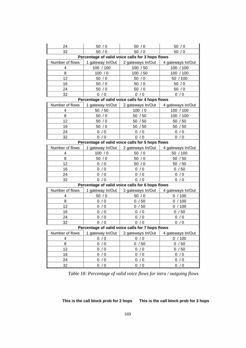
169
24 50 / 0 50 / 0 50 / 0 32 50 / 0 50 / 0 50 / 0
Percentage of valid voice calls for 3 hops flows Number of flows 1 gateway In/Out 2 gateways In/Out 4 gateways In/Out
4 100 / 100 100 / 50 100 / 100 8 100 / 0 100 / 50 100 / 100
12 50 / 0 50 / 0 50 / 100 16 50 / 0 50 / 0 50 / 0 24 50 / 0 50 / 0 50 / 0 32 0 / 0 0 / 0 0 / 0
Percentage of valid voice calls for 4 hops flows Number of flows 1 gateway In/Out 2 gateways In/Out 4 gateways In/Out
4 50 / 50 100 / 0 100 / 100 8 50 / 0 50 / 50 100 / 100
12 50 / 0 50 / 50 50 / 50 16 50 / 0 50 / 50 50 / 50 24 0 / 0 0 / 0 0 / 0 32 0 / 0 0 / 0 0 / 0
Percentage of valid voice calls for 5 hops flows Number of flows 1 gateway In/Out 2 gateways In/Out 4 gateways In/Out
4 100 / 0 50 / 0 50 / 100 8 50 / 0 50 / 0 50 / 50
12 0 / 0 50 / 0 50 / 50 16 0 / 0 0 / 0 0 / 50 24 0 / 0 0 / 0 0 / 0 32 0 / 0 0 / 0 0 / 0
Percentage of valid voice calls for 6 hops flows Number of flows 1 gateway In/Out 2 gateways In/Out 4 gateways In/Out
4 50 / 0 50 / 0 0 / 100 8 0 / 0 0 / 50 0 / 100
12 0 / 0 0 / 50 0 / 100 16 0 / 0 0 / 0 0 / 50 24 0 / 0 0 / 0 0 / 0 32 0 / 0 0 / 0 0 / 0
Percentage of valid voice calls for 7 hops flows Number of flows 1 gateway In/Out 2 gateways In/Out 4 gateways In/Out
4 0 / 0 0 / 0 0 / 100 8 0 / 0 0 / 50 0 / 50
12 0 / 0 0 / 0 0 / 50 16 0 / 0 0 / 0 0 / 0 24 0 / 0 0 / 0 0 / 0 32 0 / 0 0 / 0 0 / 0
Table 18: Percentage of valid voice flows for intra / outgoing flows
This is the call block prob for 2 hops This is th e call block prob for 3 hops
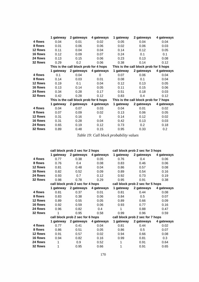
170
1 gateway 2 gateways 4 gateways 1 gateway 2 gateway s 4 gateways 4 flows 0.04 0.01 0.02 0.05 0.04 0.04 8 flows 0.01 0.06 0.06 0.02 0.06 0.03 12 flows 0.11 0.04 0.04 0.14 0.12 0.05 16 flows 0.12 0.09 0.07 0.24 0.1 0.1 24 flows 0.13 0.15 0.06 0.23 0.13 0.08 32 flows 0.29 0.2 0.06 0.38 0.14 0.12
This is the call block prob for 4 hops This is t he call block prob for 5 hops 1 gateway 2 gateways 4 gateways 1 gateway 2 gatewa ys 4 gateways
4 flows 0.1 0.04 0 0.07 0.06 0.04 8 flows 0.14 0.03 0.01 0.08 0.1 0.04 12 flows 0.19 0.1 0.04 0.12 0.13 0.05 16 flows 0.13 0.14 0.05 0.11 0.15 0.06 24 flows 0.34 0.28 0.17 0.51 0.18 0.03 32 flows 0.42 0.28 0.12 0.83 0.4 0.12
This is the call block prob for 6 hops This is t he call block prob for 7 hops 1 gateway 2 gateways 4 gateways 1 gateway 2 gatewa ys 4 gateways
4 flows 0.04 0.07 0.03 0.04 0.01 0.02 8 flows 0.07 0.09 0.02 0.13 0.06 0.05 12 flows 0.31 0.16 0 0.14 0.12 0.02 16 flows 0.31 0.28 0.04 0.42 0.13 0.03 24 flows 0.65 0.19 0.12 0.73 0.2 0.18 32 flows 0.89 0.48 0.15 0.95 0.33 0.2
Table 19: Call block probability values
call block prob 2 sec for 2 hops call block prob 2 sec for 3 hops 1 gateway 2 gateways 4 gateways 1 gateway 2 gatewa ys 4 gateways
4 flows 0.77 0.38 0.05 0.76 0.4 0.06 8 flows 0.76 0.4 0.08 0.83 0.46 0.06 12 flows 0.81 0.48 0.04 0.86 0.57 0.08 16 flows 0.82 0.52 0.09 0.89 0.54 0.16 24 flows 0.93 0.7 0.12 0.92 0.73 0.19 32 flows 0.98 0.78 0.29 0.95 0.91 0.38
call block prob 2 sec for 4 hops call block prob 2 sec for 5 hops 1 gateway 2 gateways 4 gateways 1 gateway 2 gatewa ys 4 gateways
4 flows 0.81 0.37 0.01 0.81 0.44 0.08 8 flows 0.83 0.38 0.06 0.84 0.5 0.07 12 flows 0.89 0.55 0.05 0.89 0.66 0.09 16 flows 0.92 0.59 0.06 0.93 0.77 0.16 24 flows 0.96 0.82 0.4 1 0.88 0.47 32 flows 1 0.95 0.58 0.99 0.96 0.59
call block prob 2 sec for 6 hops call block prob 2 sec for 7 hops 1 gateway 2 gateways 4 gateways 1 gateway 2 gateway s 4 gateways
4 flows 0.77 0.41 0.04 0.81 0.44 0.02 8 flows 0.86 0.51 0.05 0.86 0.5 0.07 12 flows 0.91 0.57 0.02 0.94 0.66 0.08 16 flows 0.94 0.82 0.16 0.99 0.81 0.3 24 flows 1 0.9 0.52 1 0.91 0.64 32 flows 1 0.95 0.66 1 0.91 0.65

171
Table 20: Call block probability within 2 seconds values
call block prob 5 sec for 2 hops call block prob 5 sec for 3 hops 1 gateway 2 gateways 4 gateways 1 gateway 2 gateway s 4 gateways
4 flows 0.11 0.03 0.02 0.13 0.04 0.05 8 flows 0.14 0.13 0.06 0.11 0.07 0.03 12 flows 0.26 0.1 0.04 0.33 0.17 0.05 16 flows 0.31 0.19 0.07 0.45 0.17 0.12 24 flows 0.59 0.32 0.06 0.7 0.35 0.09 32 flows 0.75 0.44 0.13 0.87 0.57 0.16
call block prob 5 sec for 4 hops call block prob 5 sec for 5 hops 1 gateway 2 gateways 4 gateways 1 gateway 2 gateway s 4 gateways
4 flows 0.16 0.05 0.01 0.15 0.08 0.04 8 flows 0.25 0.07 0.02 0.29 0.16 0.04 12 flows 0.34 0.18 0.04 0.38 0.22 0.05 16 flows 0.44 0.22 0.05 0.62 0.31 0.07 24 flows 0.76 0.54 0.22 0.94 0.65 0.16 32 flows 0.86 0.72 0.23 0.98 0.77 0.27
call block prob 5 sec for 6 hops call block prob 5 sec for 7 hops 1 gateway 2 gateways 4 gateways 1 gateway 2 gateway s 4 gateways
4 flows 0.11 0.07 0.04 0.16 0.03 0.02 8 flows 0.31 0.12 0.02 0.42 0.11 0.05 12 flows 0.61 0.26 0 0.53 0.25 0.02 16 flows 0.75 0.47 0.04 0.87 0.41 0.07 24 flows 1 0.64 0.19 0.98 0.65 0.35 32 flows 1 0.87 0.4 1 0.76 0.34
Table 21: Call block probability within 5 seconds values
call block prob 10 sec for 2 hops call block prob 10 sec for 3 hops 1 gateway 2 gateways 4 gateways 1 gateway 2 gateway s 4 gateways
4 flows 0.04 0.01 0.02 0.05 0.04 0.05 8 flows 0.01 0.06 0.06 0.03 0.06 0.03 12 flows 0.14 0.05 0.04 0.17 0.12 0.05 16 flows 0.15 0.09 0.07 0.32 0.1 0.11 24 flows 0.3 0.2 0.06 0.49 0.18 0.08 32 flows 0.66 0.3 0.1 0.72 0.4 0.13
call block prob 10 sec for 4 hops call block prob 10 sec for 5 hops 1 gateway 2 gateways 4 gateways 1 gateway 2 gateway s 4 gateways
4 flows 0.11 0.04 0.01 0.08 0.06 0.04 8 flows 0.17 0.03 0.02 0.11 0.1 0.04 12 flows 0.23 0.1 0.04 0.22 0.14 0.05 16 flows 0.24 0.17 0.05 0.42 0.19 0.06 24 flows 0.59 0.42 0.18 0.83 0.44 0.08 32 flows 0.79 0.59 0.18 0.96 0.7 0.2
call block prob 10 sec for 6 hops call block prob 10 sec for 7 hops 1 gateway 2 gateways 4 gateways 1 gateway 2 gateway s 4 gateways

172
4 flows 0.04 0.07 0.04 0.07 0.01 0.02 8 flows 0.1 0.11 0.02 0.21 0.06 0.05 12 flows 0.45 0.18 0 0.29 0.17 0.02 16 flows 0.54 0.36 0.04 0.72 0.28 0.04 24 flows 0.9 0.49 0.17 0.96 0.48 0.25 32 flows 0.99 0.8 0.21 1 0.69 0.3
Table 22: Call block probability within 10 seconds values
D Graphs
D.1 About voice traffic flows
D.1.1 End to end delay
D.1.1.1 Average end to end delay plotted by gateways
For one gateway simulations
For two gateways simulations

173
For four gateways simulations
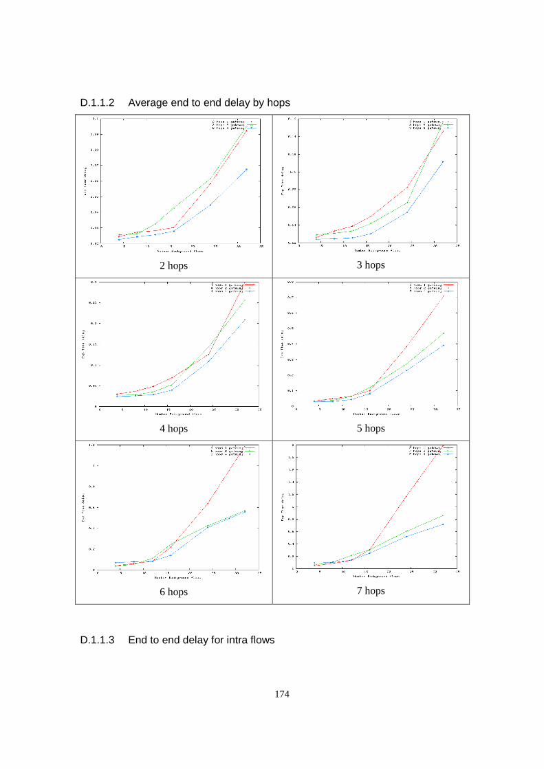
174
D.1.1.2 Average end to end delay by hops
2 hops
3 hops
4 hops
5 hops
6 hops
7 hops
D.1.1.3 End to end delay for intra flows

175
2 hops
3 hops
4 hops
5 hops
6 hops
7 hops
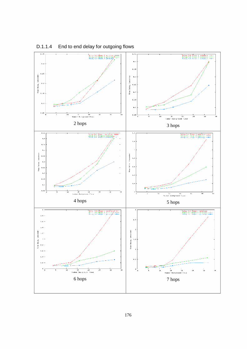
176
D.1.1.4 End to end delay for outgoing flows
2 hops
3 hops
4 hops
5 hops
6 hops
7 hops
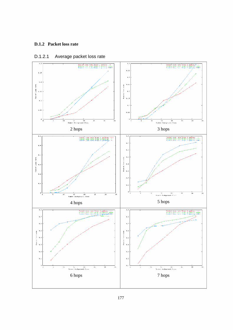
177
D.1.2 Packet loss rate
D.1.2.1 Average packet loss rate
2 hops
3 hops
4 hops
5 hops
6 hops
7 hops

178
D.1.2.2 Packet loss rate for intra flows
2 hops
3 hops
4 hops
5 hops
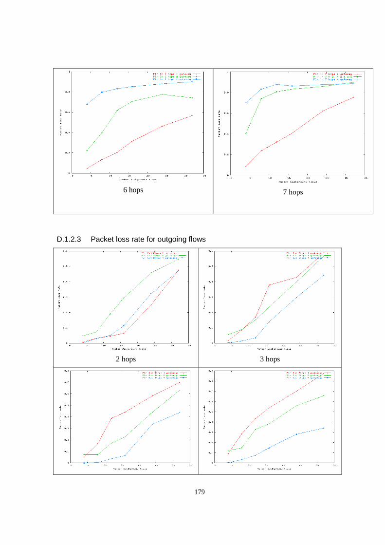
179
6 hops
7 hops
D.1.2.3 Packet loss rate for outgoing flows
2 hops
3 hops
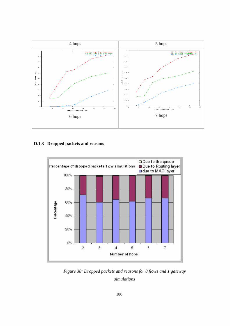
180
4 hops 5 hops
6 hops
7 hops
D.1.3 Dropped packets and reasons
Figure 38: Dropped packets and reasons for 8 flows and 1 gateway
simulations
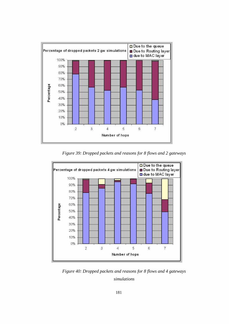
181
Figure 39: Dropped packets and reasons for 8 flows and 2 gateways
Figure 40: Dropped packets and reasons for 8 flows and 4 gateways
simulations

182
D.2 About SIP
D.2.1 SIP call setup
2 hops background flows
3 hops background flows
4 hops background flows
5 hops background flows
6 hops background flows
7 hops background flows

183
D.2.2 Calls accepted each 100 milliseconds
This graphs show how much per cent of the accepted calls are accepted each 100
milliseconds.
2 hops 4 background flows
2 hops 8 background flows
2 hops 12 background flows
2 hops 16 background flows
2 hops 24 background flows
2 hops 32 background flows
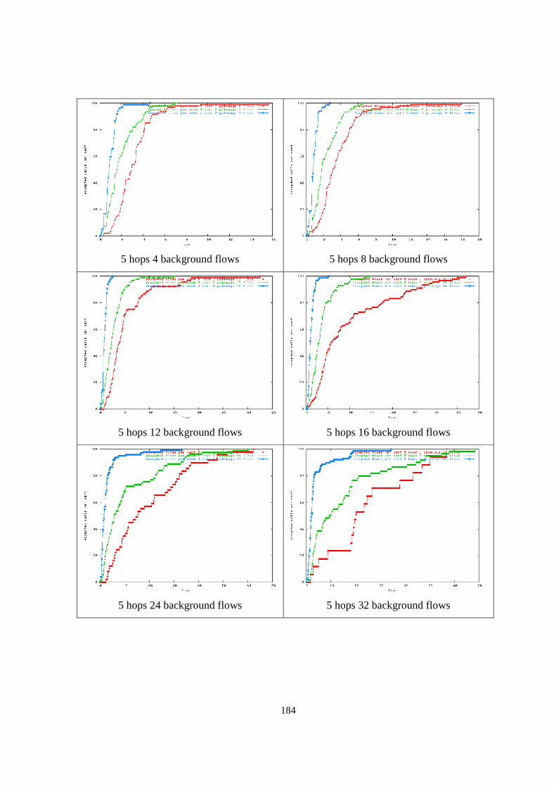
184
5 hops 4 background flows
5 hops 8 background flows
5 hops 12 background flows
5 hops 16 background flows
5 hops 24 background flows
5 hops 32 background flows
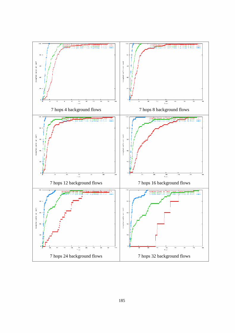
185
7 hops 4 background flows
7 hops 8 background flows
7 hops 12 background flows
7 hops 16 background flows
7 hops 24 background flows
7 hops 32 background flows
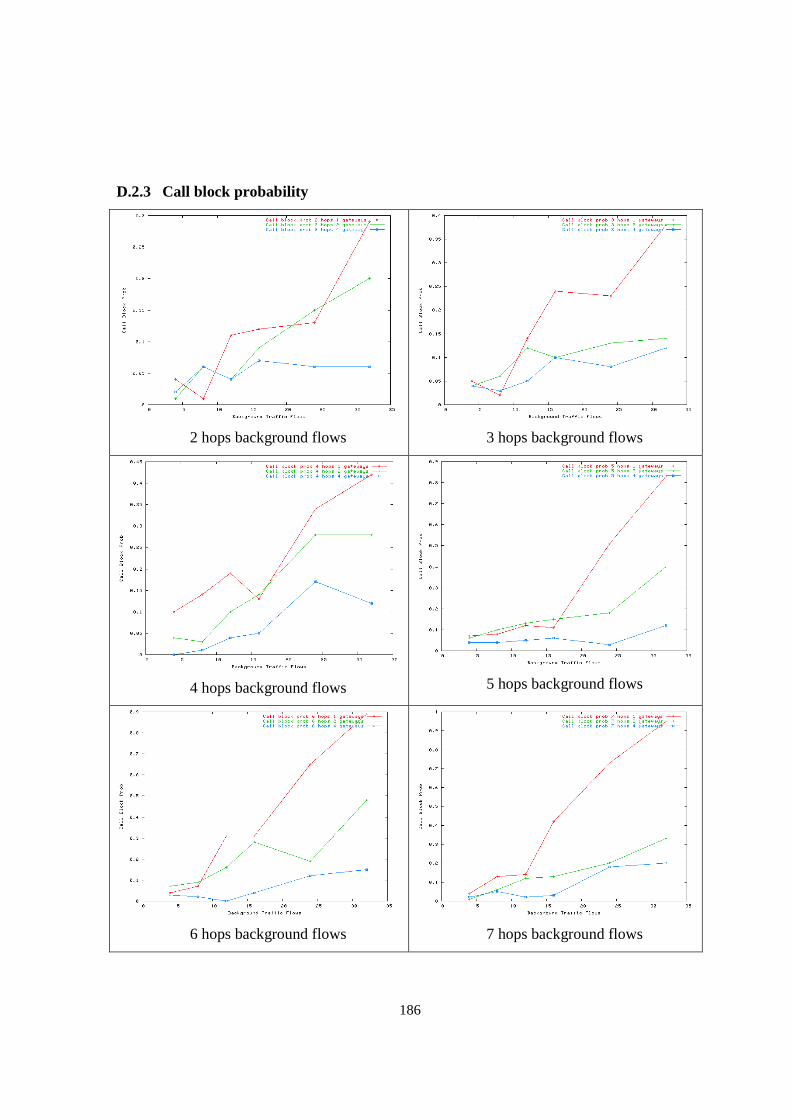
186
D.2.3 Call block probability
2 hops background flows
3 hops background flows
4 hops background flows
5 hops background flows
6 hops background flows
7 hops background flows
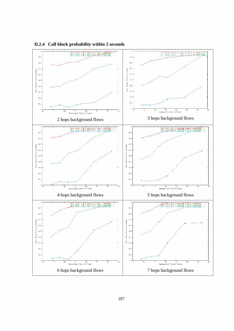
187
D.2.4 Call block probability within 2 seconds
2 hops background flows
3 hops background flows
4 hops background flows
5 hops background flows
6 hops background flows
7 hops background flows

188
D.2.5 Call block probability within 10 seconds
2 hops background flows
3 hops background flows
4 hops background flows
5 hops background flows
6 hops background flows
7 hops background flows

189
D.2.6 SIP invitation attempts
2 hops background flows
3 hops background flows
4 hops background flows
5 hops background flows
6 hops background flows
7 hops background flows
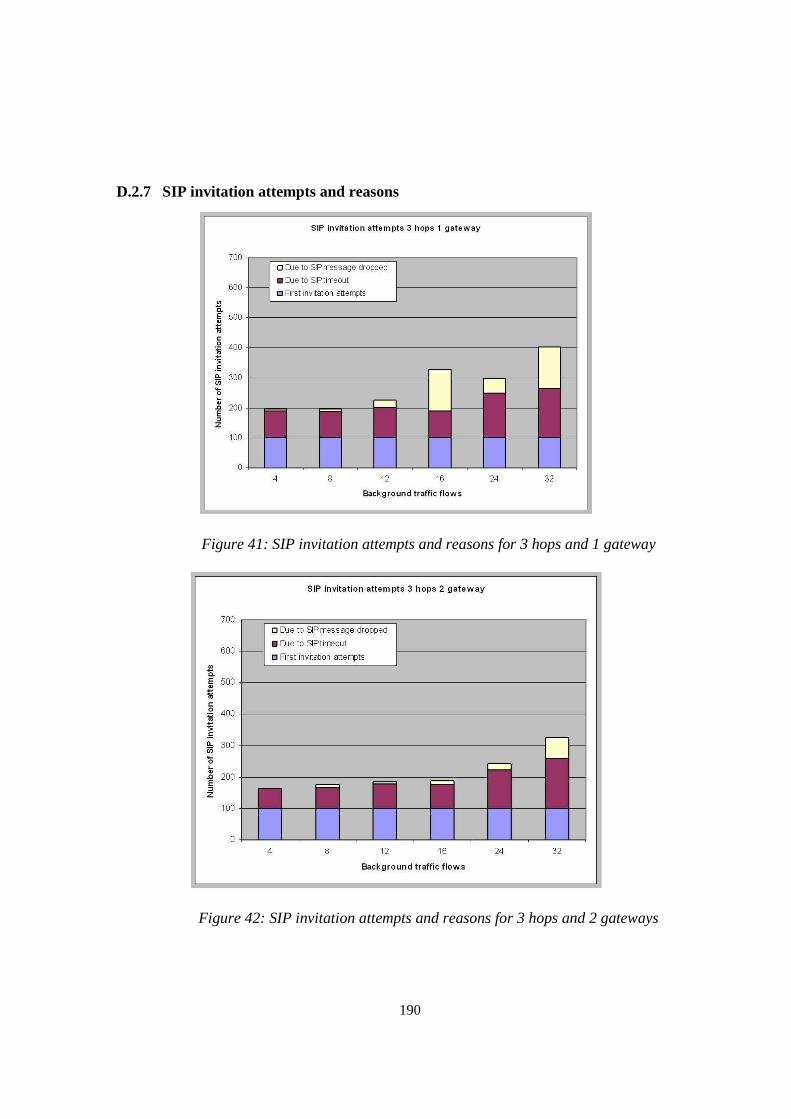
190
D.2.7 SIP invitation attempts and reasons
Figure 41: SIP invitation attempts and reasons for 3 hops and 1 gateway
Figure 42: SIP invitation attempts and reasons for 3 hops and 2 gateways
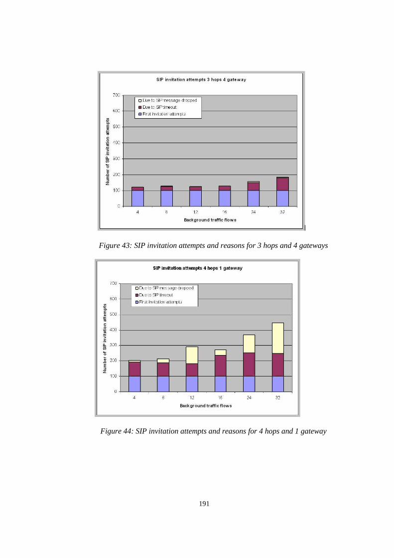
191
Figure 43: SIP invitation attempts and reasons for 3 hops and 4 gateways
Figure 44: SIP invitation attempts and reasons for 4 hops and 1 gateway

192
Figure 45: SIP invitation attempts and reasons for 4 hops and 2 gateways
simulations
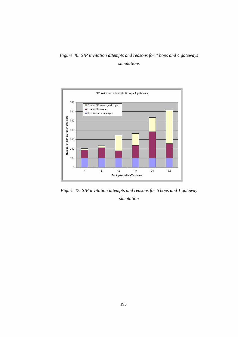
193
Figure 46: SIP invitation attempts and reasons for 4 hops and 4 gateways
simulations
Figure 47: SIP invitation attempts and reasons for 6 hops and 1 gateway
simulation
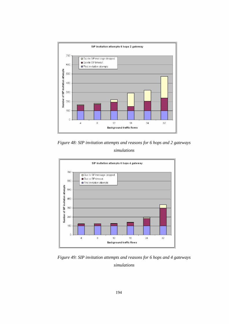
194
Figure 48: SIP invitation attempts and reasons for 6 hops and 2 gateways
simulations
Figure 49: SIP invitation attempts and reasons for 6 hops and 4 gateways
simulations

195
D.2.8 SIP number of hops
2 hops background flows
3 hops background flows
4 hops background flows
5 hops background flows
6 hops background flows
7 hops background flows

196