1

Performance Pay and the Gender Wage Gap in Spain ∗

Sara de la Rica*, Juan J. Dolado** & Raquel Vegas***

(*) Universidad del País Vasco, FEDEA & IZA

(**) Universidad Carlos III & CEPR & IZA

(***) FEDEA

May 12, 2010 (preliminary)

ABSTRACT

This paper uses detailed information from a large wage survey in 2006 to analyze the gender wage gap in the performance–pay component of total hourly wages and its contribution to the overall gender in Spain. Under the assumption that performance-pay compensation is determined in a more competitive fashion than the other components of the wage, one would expect, in principle, to find a low gender gap in the first component. However, this is not what we find. After controlling for observable differences in individual and job characteristics as well as for non random selection, the estimate of the adjusted gender gap in performance pay is around 26 log points, and that it displays a “glass ceiling” pattern. After examining alternative theories that could rationalize these findings, we conjecture that monopsonistic features, possibly related to women´s lower mobility due to housework, may be more consistent with our results than other theories related to occupational segregation.

JEL Classification: J31, J33, J42, J71.

Keywords: performance pay, gender gaps, selection bias, quantile regressions

∗ This paper has been prepared for the 2010 FEDEA Monograph Annual Conference on Talent, Effort and Social Mobility, U. Pompeu Fabra, may 19-20, 2010. We are grateful to Daniel Parent for useful comments on a preliminary version of the paper. The first two authors gratefully acknowledge financial support from the Spanish Ministry of Education (ECO2009-10818; SEC2004-04101), Consolider Ingenio-2010 (MCINN) and Consejería de Educación de la Comunidad de Madrid (Excelecon project).

Corresponding author: Sara de la Rica (sara.delarica@ehu.es).

2

1. Introduction

One of the cornerstones of the standard competitive model of the labour market

is the well-known equilibrium condition equating wages to marginal revenue products

(MRP henceforth). Accordingly, the final wage distribution represents the equilibrium

outcome of demand and supply forces. This straightforward implication of the

competitive model has proven instrumental in the empirical analysis of how relevant

phenomena, such as changes in the relative demand and supply of skills have affected

within and between-group wage inequality over the last few decades in economies with

flexible labour markets, like e.g., UK and US (see, eg., Katz and Murphy, 1992). Yet, it is

also well established that the competitive model can provide a rather misleading

interpretation of how wages are actually determined in real-life labour markets when

information is asymmetric or search frictions are present in the allocation of workers to

jobs. In addition, a common feature of many existing labour market institutions (like

unions and minimum wages) is that they tend to compress the wage distribution and

thus reduce pay differences between more productive and less productive workers.1

While it is reasonable to acknowledge that the competitive paradigm often lacks

realism in describing how wages are set, there are some specific forms of wage

compensation that could be considered as good proxies of the “wage equals MRP”

condition. In particular, if compensation is paid at least partially as a function of

performance pay – such as bonuses, comission or piece rates- it seems plausible to assume

that this wage component becomes closer to worker´s productivity than the remaining

components (e.g.,the base wage) that do not depend so closely on individual

performance. Following this intuitive reasoning, Lemieux et al. (2009) have analyzed

the impact of performance pay (PP hereafter) on wage inequality in the US . Their basic

hypothesis is that, through a widespread reduction in the cost of gathering and

processing information, PP growing incidence may have contributed to the increase in

inequality, mainly at the top of the wage distribution. Indeed, their finding that PP

1 Empirical evidence, such as Beaudry and DiNardo (1991), Card (1996), DiNardo et al. (1996), Farber and Gibbons (1996), and Lemieux (1998) provide ample evidence about the different channels through which wages are not equalized to their MRPs.

3

accounts for 25% of male wage inequality between the late 1970s and early 1980s

provides favourable support for this conjecture. 2

In this paper, we contribute to this line of research by making use of a recently

available dataset on the detailed breakdown of total wage compensation for Spanish

workers into its different components. We re-examine Lemieux et al. ´s (2009)

hypothesis, but from a different angle which, to our knowledge, is somewhat novel in

this literature.3 Specifically, we analyze whether PP compensation differs by gender

and the extent to which this component contributes to explaining the overall wage

gender gap (gender gap hereafter) in Spain.

One could think of two alternative hypotheses regarding gender differences in PP.

On the one hand, under the presumption that this component is determined in a more

competitive fashion than the remaining components of the wage, the gender gap in PP

between equally skilled men and women could be smaller than in the non PP

components. In other words, since in theory PP responds mostly to meritocracy, equally

performing workers should receive the same PP irrespectively of their gender.

Moreover, if women perceive some forms of (taste and/or statistical) discrimination in

non-PP jobs relative to men, then they will seek intensively for PP jobs in order to

ameliorate these disadvantages. However, against this hypothesis one could claim that,

to the extent that effort at the marketplace may be negatively affected by housework, PP

could also provide a clear channel through which women´ s greater involvement in

household tasks hinders their returns in the labour market and therefore lower their PP

relative to men ´s. 4 For example, Amuedo-Dorantes and de la Rica (2006) find that

variable wage complements in Spain, which can easily make up to 40 percent of men's

wages - account for up to 80 percent of the aggregate gender gap due partially to

women ´s lower availability to undertake long working hours.

2 The existing literature has mainly focused on analyses of the incentive effects on productivity of PP arrangements; see, inter alia, Booth (1999), Ewing (1996), Dohmen and Falk (2009) and Lazear (2000), among others. 3 There is however a growing literature on gender differences in compensation for CEOs and top executives which shares element in common with performance pay (see, e.g., Bertrand and Hallock, 2001, and Bertrand et al., 2009) 4 See Becker (1985) and a stylized model with this flavour in Appendix 2 (A).

4

On the other hand, even abstracting from the role of distorting labour market

institutions, the assumptions of free access to PP jobs and/or the absence of search

frictions in a competitive setup may not be suitable for female workers. First, as has

been stressed in the occupational segregation literature, women may select themselves

into non-PP jobs (e.g. public sector jobs) because they anticipate that these positions are

more compatible with their larger household responsibilities. Hence, in line with the so-

called mommy track hypothesis (see Mincer and Polacheck, 1977), they may willingly opt

for jobs entailing steadier and, possibly, lower pay in exchange for less penalties in case

of career interruptions. Secondly, employers may be more reluctant to place women in

fast-track jobs involving PP if they expect lower female work attachment even though

the have the same ability distribution as their male colleagues (see Lazear and Rosen,

1990). Thirdly, statistical discrimination in the allocation of PP jobs may still prevail if

employers invest on workers´ specific training and therefore try to minimize quits.

Moreover, if women are aware of the existence of statistical discrimination in advance,

this may discourage them from applying to these jobs leading to self-fulfilling equilibria

(see Coate and Loury, 1993, and de la Rica et al., 2009). Lastly, the presence of some

monopsonistic features in PP jobs, due to women´ s lower mobility or lack of alternative

job offers, should not be discarded even if, contrary to the standard human capital

explanation, this does not lead to lower productivity (see Booth et al., 2003, and

Manning, 2003).

In view of these considerations, our goal in this paper is to dig deeper into the

specific role played by PP as a determinant of the overall gender gap in Spain. Our data

comes from the recently released 2006 wave of the Spanish Earnings Structure Survey

which contains detailed micro-data information on the various components of the

wage, such as the base wage, overtime pay and other wage complements. When

compared to the longitudinal dataset used by Lemieux et al. (2009) - i.e., the interview

years 1976-1999 of the PSID- our data suffers from a clear drawback since its cross-

section nature prevents us from controlling for workers´ fixed effects. In exchange,

however, it has the advantage of providing information about the precise amount of PP

received by workers, in contrast to PSID which only reports qualitative information on

whether employees receive a variable pay component as part of their total

5

compensation at least once during their employment relationships (but not its amount).

This implies that our data are less noisy than theirs and that we can focus specifically on

the PP component rather than on jobs that pay PP, as Lemieux et al. (2009) do.

In the first half of the paper, we address the impact of PP on the observed gender

gap in total pay both at the mean and throughout the wage distribution, since PP is

bound to have substantially different effects at different percentiles. In effect, if PP is

more concentrated at the higher quantiles, where bonuses and commissions are

believed to represent a more important fraction of compensation, they may have a

larger impact on the gender gap and therefore help explain at least partly the so-called

“glass ceiling” effect at the top of the wage distribution. The second part focuses

exclusively on the PP wage component and explores whether there are potential

selection issues in the fraction of employees receiving PP, and to what extent the pattern

observed for raw gender gaps changes once observable individual controls and

selectivity biases are accounted for. Additionally, we present evidence about adjusted

gender PP gaps within-firms and within-occupations in order to disentangle the role

played by different theories explaining the existence of sizeable adjusted gaps.

The rest of the paper is organized as follows. Section 2 describes the dataset

and provides some basic descriptive statistics regarding the whole sample, the

distribution and extent of PP, the differences between the characteristics of workers

receiving and not receiving PP, and the contribution of the gender gap in PP to the

overall gender gap in raw terms. In Section 3, we test whether the PP wage component

is set in a more competitive way than the non-PP component. Section 4 deals with

adjusted gaps in PP jobs. After addressing the issue of nonrandom selection among

workers participating in PP jobs, we analyze which of the different explanations for

gender gaps fits better with the evidence. Section 5 allows for different returns on

observable characteristics by gender in order to identify which specific traits are

differently rewarded in the market place. Finally, Section 6 concludes.

6

2. Data and descriptive statistics

Our data source is the third wave of the Spanish Earnings Structure Survey

(Encuesta de Estructura Salarial or ESS 06 in short).5 The ESS is the outcome of a

European Project aiming at the design of harmonized earnings databases for several

European countries. The survey is based on two-stage random samples of workers from

establishments in the manufacturing, construction and service industries. First,

establishments are randomly selected from the Social Security General Register of

Payments records, which are stratified by region and establishment size. In a second

stage, samples of workers from each of the selected establishments are also randomly

drawn. Overall, sample sizes are much larger than those provided by any other

Spanish survey (see below for details). Besides wage compensation, EES collects

individual information on workers’ demographics (such as age and educational

attainment) and job characteristics (including industry, occupation, contract type, type

of collective bargaining, establishment’ s export activity, establishment size, and

region).

The main advantages of EES 06 relative to its earlier waves are that: (i)

establishments with less than 10 employees are included in this survey whereas only

employees in larger establishments were previously interviewed; (ii) it includes a

module where employers provide detailed information on the breakdown into fixed

and variable components of the total annual wage compensation paid to their workers.

This module allows us to identify PP, since data on annual bonuses and commissions

related to productivity are specifically reported for each employee. One important

shortcoming, however, is that, since the latter information is directly provided by

employers rather than by workers and the structure of EES does not enable us to

construct a matched employer-employee dataset, information on either workers´ civil

status, spouses´ characteristics or the number and age of children in the households is

not available.

More concretely, besides reporting total monthly gross wages and working

hours, EES 06 does provide information on both the ordinary (base wage and other

5 The previous waves correspond to 1995 and 2002.

7

complements due to shifts, tenure, job risks, etc.) and non-ordinary components of

annual gross earnings. Regarding the latter category, the ESS 06 distinguishes between

two different types of payments:

• Fixed Annual Non-ordinary Payments. This payment “basically

corresponds to extraordinary compensations at Christmas and summer

vacations (in Spanish, known as pagas por navidad y verano) 6, the standard

rates for overtime work and participation in firms´ normal profits”. It is

specifically stated that their amount is known in advance by the

employee, typically established at the collective bargaining level, and that

they do not depend on either workers´ or firms´ performance.

• Variable Annual Non-ordinary Payments. In contrast to the first category,

these are “payments related to workers´ or firms´ performance whose

amount is not established a priori since it depends on incentives, returns

and extraordinary profits”. It lumps together bonuses, compensations and

piece rates.

Given this breakdown of total wage compensation, the PP component in the

sequel will correspond to the Variable Annual Non-ordinary Payments whereas the non-

PP components will be identified as the sum of the ordinary wage and the Fixed Annual

Non-ordinary Payments.

2.1. Description of the dataset

Our sample consists of full-time workers aged 18-65 for whom the interview

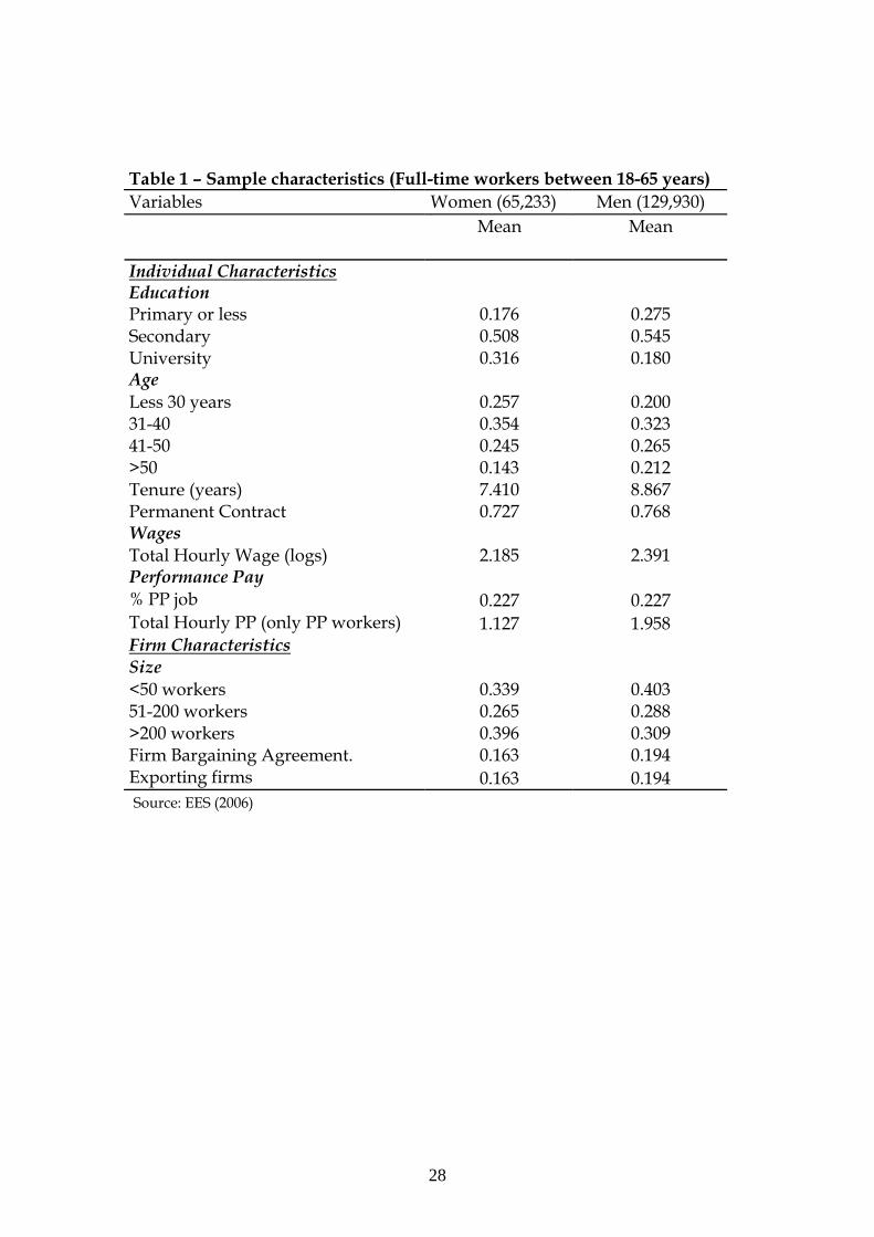
month (october) is an ordinary period regarding their labour status. Table 1 displays the

weighted descriptive statistics for the male and female samples. They contain a total of

129,930 males (66.6%) and 65,223 females (33.4%) covering almost 18,000

establishments.

[Table 1 about here]

6 This implies that the fixed part of the total annual gross wage is distributed into 12 ordinary instalments and 2 extraordinary ones. This tradition dates back to the Francoist industrial relations during the dictatorship period.

8

Inspection of workers´ demographic characteristics reveals the following

stylized facts: (i) women´ s educational attainments are significantly larger than men´ s

– e.g., the percentage of female workers with a university degree (32%) almost doubles

men’s (18%) whereas the fraction of women with at most primary education is 10 pp.

smaller (18% vs. 28%) than men´s , (ii) women are about two years younger than men

(from interpolation of the mid-points of the different age brackets), (iii) female job

tenure is about 1.5 years shorter than males´ tenure, and (iv) the raw gender gap is

about 21 log points in favour of male workers. As regards firms´ characteristics, on

average, women work in larger establishments (> 200 employees) than men (a 9 pp.

higher share), and enjoy a lower coverage by bargaining agreements at the firm level (3

pp. less).

Regarding total gross hourly wages, the gender gap in favour of men is about 21

log points, using differences in mean logged wages, and 23.1%, using the ratio of the

wage levels.7 Interestingly, the incidence of PP (22.7 %) is almost identical across

genders which, prima facie, is consistent with our previous conjecture that this kind of

jobs are attractive to women because, in principle, they should be less subject to

discriminatory practices. This statement, however, will need to be reconsidered later on,

once we report further evidence on the distribution of women throughout the PP

distribution.

2.2. Characterization of performance pay

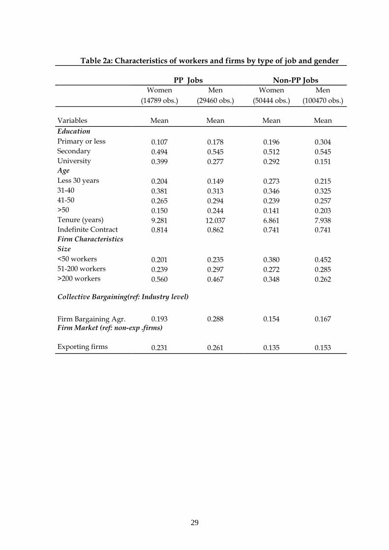
Table 2a compares the sample characteristics of workers and firms in PP and

non-PP jobs, distinguishing by gender. The main finding is that workers on PP jobs are

more educated than those in non-PP jobs (40% of women and 27% of men in the PP

sample have a university degree against 29% and 15% in the non-PP sample). Likewise,

they are older (about a 10 pp. larger share in the 31-50 age category), have longer tenure

(about 2.5 years longer for women and 5 years for men), enjoy a higher rate of

7 Denoting the total annual gross wage by GAW, total hourly wages are defined as w= GAW /ORH+OVH), where ORH represents annual ordinary working hours set at the collective bargaining agreement (jornada anual pactada) and OVH denotes the overtime working hours completed in the month of the interview (october). The latter are annualized using the seasonal pattern of aggregate extra hours in the Spanish economy as of 2006.

9

permanent contracts and work in larger establishments (typically less subject to

centralized bargaining levels).

Table 2b, in turn, presents the incidence of PP jobs by industry and occupation.

Regarding industries, Financial Intermediation (60%) and Education (9%) are the sectors

where PP is most and least prevalent, respectively. As for occupations, the results

confirm that PP incidence is much higher for the high-wage categories: 50% for

managers and 30% for Professionals and Technicians.

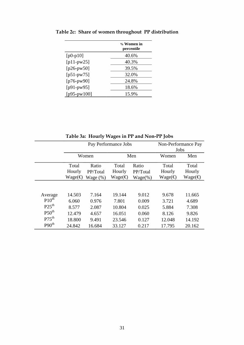
Finally, Table 2c reports the share of female workers receiving PP throughout the

distribution of this component of the wage, which we can compare to the average share

of women receiving PP in our sample, i.e., about 35% (=14798/ 44249). The sharp

decline in this proportion as we move upward in the PP distribution - from 41% at the

bottom to 16% at the top- is seemingly inconsistent with the above-mentioned

conjecture about more skilled women being more likely to seek jobs entailing PP

compensation, especially since, as reported above, they have higher educational

attainments than men. By contrast, such evidence would be consistent with the

implications of theories based on occupational segregation and/or lower mobility

which predict a “glass “ceiling “pattern whereby well qualified females are less likely to

get better paid positions than high qualified males.

[Tables 2a, b and c about here]

2.3. The Contribution of Performance Pay to the Overall Gender Gap

We next analyze how important is PP, the size of the gender gap in this wage

component and, finally, its contribution to the overall gender gap. As explained in

Appendix 1, the computation of the respective contributions of the gender gaps in the

PP and non-PP components to the overall gender gap is greatly facilitated by using a

measure of the gap expressed in percent (i.e., the ratio between average male and

female wage minus unity) rather than in log points (differences in average logged

wages), as is customary in the literature. The first four columns in Table 3a present the

total hourly wage compensation in PP jobs (expressed in €) across genders and the

corresponding shares of total wages accounted by the PP component. Further, for

10

comparison, the hourly wages in non-PP jobs appear in the last two columns. Table 3b

reports similar evidence but this time referred to the two components of the wage

compensation received by PP workers, i.e. its variable and non-variable components.

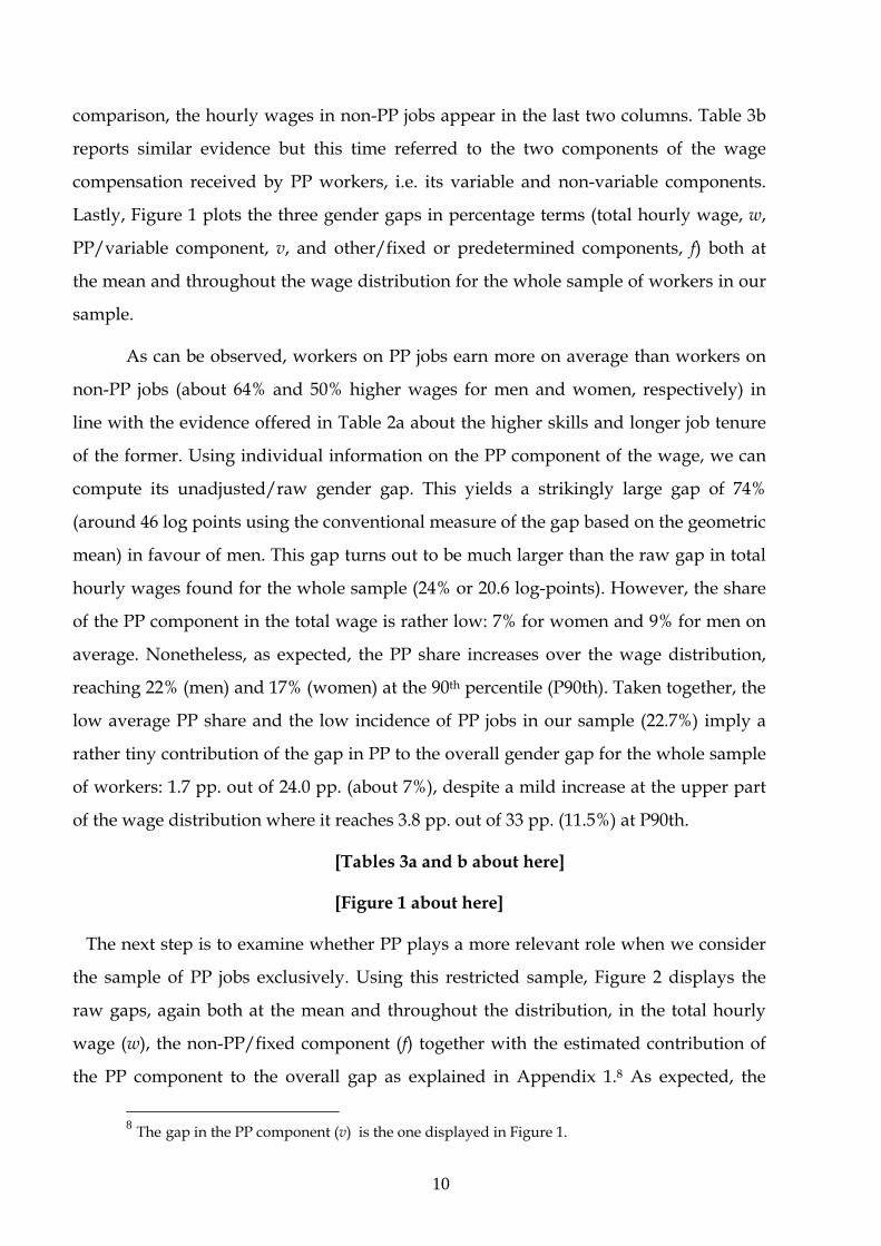
Lastly, Figure 1 plots the three gender gaps in percentage terms (total hourly wage, w,

PP/variable component, v, and other/fixed or predetermined components, f) both at

the mean and throughout the wage distribution for the whole sample of workers in our

sample.

As can be observed, workers on PP jobs earn more on average than workers on

non-PP jobs (about 64% and 50% higher wages for men and women, respectively) in

line with the evidence offered in Table 2a about the higher skills and longer job tenure

of the former. Using individual information on the PP component of the wage, we can

compute its unadjusted/raw gender gap. This yields a strikingly large gap of 74%

(around 46 log points using the conventional measure of the gap based on the geometric

mean) in favour of men. This gap turns out to be much larger than the raw gap in total

hourly wages found for the whole sample (24% or 20.6 log-points). However, the share

of the PP component in the total wage is rather low: 7% for women and 9% for men on

average. Nonetheless, as expected, the PP share increases over the wage distribution,

reaching 22% (men) and 17% (women) at the 90th percentile (P90th). Taken together, the

low average PP share and the low incidence of PP jobs in our sample (22.7%) imply a

rather tiny contribution of the gap in PP to the overall gender gap for the whole sample

of workers: 1.7 pp. out of 24.0 pp. (about 7%), despite a mild increase at the upper part

of the wage distribution where it reaches 3.8 pp. out of 33 pp. (11.5%) at P90th.

[Tables 3a and b about here]

[Figure 1 about here]

The next step is to examine whether PP plays a more relevant role when we consider

the sample of PP jobs exclusively. Using this restricted sample, Figure 2 displays the

raw gaps, again both at the mean and throughout the distribution, in the total hourly

wage (w), the non-PP/fixed component (f) together with the estimated contribution of

the PP component to the overall gap as explained in Appendix 1.8 As expected, the

8 The gap in the PP component (v) is the one displayed in Figure 1.

11

contribution of PP to the aggregate hourly wage gap is now higher than in the whole

sample reaching , on average, 5.7 pp. out of 32 pp. (i.e., about 18%) and 11.7 pp. out of

46.5 pp. (25%) at the top of the distribution.

In sum, two main conclusions stem from this preliminary evidence: (I) the gender

gap in PP is much larger than in total hourly wage compensation, particularly at the top

of the wage distribution where it can explain about one-fourth of the “glass ceiling”

pattern observed at the higher percentiles, and (II) PP makes a dent at higher wages in

line with the previous evidence that workers receiving this type of variable

compensation have better observable characteristics.

In principle, several theories would be consistent with the above-mentioned

results. First, as regards finding (I), it is likely that wages set in collective bargaining at

the sectoral (provincial-, industry-wide) level and actual wages are similar for non-

college workers in less-skilled/blue-collar occupations, while bargained wages do not

bind for college workers in high skill/ white collar occupations. There is evidence (see

Dolado et al., 1997) pointing out that employers in Spain improve high-skill workers´

pay above compressed bargained wages through formal and informal agreements

which are likely to involve variable PP arrangements. Therefore, insofar as unions

compress the wage distribution and base wages respond more to occupational

categories and tenure than to individual characteristics, like gender, it is likely that the

raw non-PP gender gap would be quite smaller than the raw PP gap. This is confirmed

by the fact that the standard deviation of the (logged) fixed component of total hourly

wages (0.61 and 0.60 for men and women, respectively) is less than one-half the

standard deviation of the (logged) PP component (1.41 and 1.34, respectively).

As for finding (II), it could be rationalized by either: (i) women exerting less

effort in PP jobs due to disutility of housework, (ii) women self-selecting away from PP

jobs where variable components represent a relevantshare of total compensation, or (iii)

women receiving lower PP than men due to monopsonistic features elements in the PP

segment of the labour market, possibly related to employers´ beliefs that women enjoy

lower mobility than equally qualified men.

12

Appendix 2 (A andB) offers a simple model which illustrates the main gender

implications of jobs offering PP and therefore serves as background for the discussion

of the main predictions of the above-mentioned theories throghout the sequel.

Disentangling which of the previous theories is more likely to operate in

explaining the very large gender gap found for PP requires several steps. First, Lemieux

et al.´s (2007) hypothesis that PP tends to be closer to MRP than non-PP compensation

needs to be tested. Next, we also need to examine whether the pattern of the PP raw gap

discussed above remains similar once it is adjusted for differences in individual and job

characteristics across genders. In other words, it is only under the competitive labor

market paradigm and under similar observable characteristics that the documented PP

gap can be described as being “strikingly large”. The next two sections are devoted to

address these issues.

[Figure 2 about here]

3. Is PP determined in a competitive fashion?

Following the above-mentioned motivation, we devote this section to analyze

whether PP jobs are “more attached to the worker” whereas non-PP jobs are more

“attached to the job”. The basic insight once more is that, if PP depends essentially on

individuals´ endowed and acquired characteristics, MRP would be more transferable

across firms and occupations, supporting the idea that PP is bound to be set in a more

competitive fashion than non-PP jobs. If PP jobs pay more on the basis of workers´

productivity, then human capital variables – basically age, education and, to a lesser

extent, tenure 9 -should have higher market returns in this kind of jobs than in other

jobs not involving PP. Conversely, returns to job characteristics- such as firm size,

sector, and tenure on the firm should receive a higher market reward in non-PP jobs.

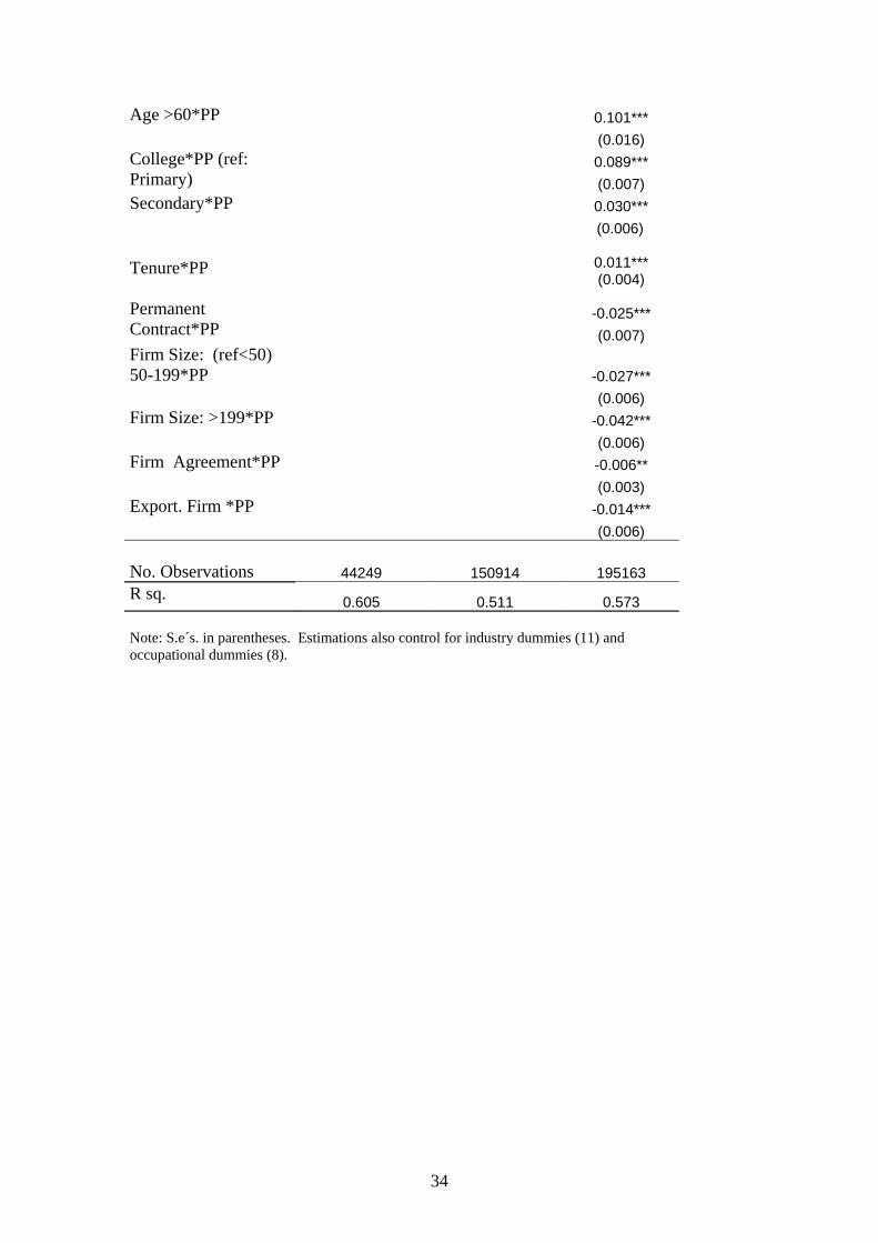
To analyze this issue, Table 4 reports standard mincerian (logged) hourly wage

regressions estimated by OLS where the returns (estimated coefficients) to job and

9 The lower (in absolute terms) coefficient on the interaction of tenure and the PP indicator may reflect high union power in collective bargaining determining the non-PP components of the wage, where tenure is a key element in wage increases.

13

human capital variables are displayed separately in the first two columns for PP and

non-PP jobs, respectively. The third last column, in turn, shows the results from a

pooled regression where interactions of human capital and job characteristics with an

indicator of receiving PP are added to test for statistically significant differences

between returns in the two samples. Thus, denoting the hourly wage of worker i in firm

j as ijW , individual and job characteristics as iX and jX , respectively, and an indicator

(1/0) for receiving PP as iD , the estimated model is:

ijjiiijiiij XDXDXXDW εφφββββ ++++++= 213210ln

where we expect 01 >φ and 02 <φ .

In line with the results by Lemieux et al. (2009), we find that the returns to

characteristics attached to the worker are larger in PP than in non-PP jobs. For example,

the returns to university and secondary education are 41% (0.304 vs. 0.215) and 60%

(0.09 vs. 0.06) larger, respectively, than in non PP jobs. Likewise, the returns to age, as a

proxy for potential experience, and to a lesser extent tenure follow the same pattern. By

contrast, the returns to firm size and other characteristics of the job are significantly

smaller in PP jobs, as is also the case for estimated coefficients on industry and

occupational dummies, not reported in this table for brevity. This evidence suports the

view that PP jobs pay wages closer to worker ‘s productivity than the rest. Yet, the fact

thatestimated returns on firm´s characteristics are, in gereneral, statistically significant

points out that workers tend to be categorized by firms into jobs, albeit less so in the

sample of workers receiving PP.

[Table 4 about here]

4. Adjusted gender gaps in the performance pay component

Once the pattern of the raw gender gap in PP has been described, we proceed

next to compute their adjusted counterparts accounting for differences in observed

individual and job characteristics. However, the fact that slightly less than one-fourth of

workers in the whole sample receive PP and that these workers present different

personal and job characteristics than non-PP workers, make us consider that non

random selection of workers into PP jobs may be a relevant issue to address. This is

14

particularly important if the selection process into PP is not exactly the same for males

and females In such a case, ignoring gender differences in selection will lead to biased

estimates of the adjusted gap for the PP component.

4.1. Selectivity issues

Table 5 presents the results of estimating a probit model to explain participation in

PP jobs (PP=1, non-PP=0). This model will be later used to compute the inverse Mill

ratio in a conventional two-stage Heckman approach to control for selection in the

estimation of log hourly wage regressions explaining the PP component. Given the lack

of information regarding civil status or number and age of children in our sample, we

use the availability of wage bargaining at the firm level (Firm Agreement) as the

identifying variable in the participation equation. The insight for this choice is that jobs

with this type of decentralized wage agreement are more likely to involve PP

compensation than other jobs where wages are set at a more centralized bargaining

level (sectoral/provincial or nationwide) and unions play a larger role. Further, the fact

that the estimated coefficient on this variable is not statistically significant when

included in the PP wage regression make us trust on the validity of this exclusion

restriction.

The first column of Table 5 presents the estimates of the coefficients in the probit

using the standard explanatory variables, where a Female indicator (1/0) captures

gender differences in the probability of receiving PP compensation. As can be observed,

women have a lower probability of getting PP than equally able men working in the

same occupations. The remaining estimates are in line with the evidence presented in

Table 2: higher educational attainment, longer tenure and being in the 31-50 age

intervals also raise this probability.

Thus, in principle, this evidence goes against the earlier conjecture that, under the

competitive labour market paradigm, equally productive men and women should not

exhibit significant differences regarding paticipation in jobs offering PP compensation

and that, if females anticipate non-competitive features in non PP jobs, they should be

more prevalent in PP jobs. To examine whether these differences in participation can be

related to women´s larger disutility in market work due to larger involvement in

15

housework, as in Becker´s hypothesis, or rather to occupational segregation and/or

lower mobility, as in the “ mommy track” and “monopsonistic” hypotheses, the second

column in Table 5 reports the estimates obtained in an specification where interaction

terms between the different age brackets and the Female dummy are added to the

model. Under the first hypothesis, the main differences againt women shoud appear

for those age groups more prone to bear household responsibilities since it is actual

involvement in housework that hampers performance in market work. Lacking

information on civil status and household composition, we choose to identify women

aged 31-50 as those more prone to be heavily involved in child bearing, looking after

elderly relatives, etc. Thus, conditioning on the remaining observable controls, one

should expect lower probability of participation for women in this age group. This

would correspond to a negative coefficient on the corresponding interaction terms

between PP and 31-39 and 40-49 brackets indicators. By contrast, under the second

hypothesis, the effect should be mainly captured by the female intercept since all

women, irrespectively of their age, antipate career interruptions due to the above-

mentioned reasons.

The basic finding is that the coefficients on these interaction terms are negative and

highly significant, pointing out that, conditioning on all the remaining covariates,

women in two above-mentioned age brackets have a lower probability of receiving PP

than younger and older women, respectively. For example, the net coefficient of a

woman aged 30-39 is -0.134 (=-0.103+0.016-0.047) whereas, for women below 30 or in

the 50-59 interval, the corresponding net coefficients would be -0.103 and -0.041 (=-

0.103-0.01+0.072), respectively. A chi-squared test rejects the null of equal coefficients

across the previous age brackets with a p-value of 0.023. Thus, this evidence points out

the “mommy track”/“monopsonistic” hypotheses are likely to play a joint role in

explaning gender differences in receiving PP.

[Table 5 about here]

16

4.2. Disentangling occupational segregation from monopsonistic features

4.2.1 Within- firms and within- occupations regressions

The next step is to analyze which of the two theories embedded in the second joint

hypothesis is more likely to explain the PP gender gap: is it “occupational segregation”

or “ monopsonistic features” ?. To try to discriminate between these two somewhat

alternative explanations, we carry out the following exercise. Using the specification of

a mincerian wage equation for the restricted sample of PP workers with a Female

intercept and equal returns to individual and job characteristics across genders, we

compare the estimated coefficient on the Female indicator in a regression (augmented by

the inverse Mills ratio obtained from the participation equation reported in the second

column of Table 5) under four different specifications: (i) a pooled regression (P), (ii)

within- occupations (WO),10 (iii) within-firms (WF), and (iv) within-firms & occupations

(WFO).

The insight for such comparison can be briefly described as follows. Let us denote the

coefficient on the Female dummy in the four specifications above as Pβ , WOβ , WFβ and

WFOβ respectively. Then, under the “occupational segregation “ hypothesis we should

expect WOβ to be significantly smaller than pβ (since we are comparing men and

women in the same occupation and firm) whereas WFβ should be similar to Pβ .

Conversely, under the “monopsonistic” hypothesis, the estimate of WFβ should be quite

smaller than the estimate of pβ (since now the comparison is between men and women

working in the same firm), while WOβ and Pβ would be similar. Finally, if both theories

play a role, then WFOβ should be below both WOβ and WFβ which, in turn, should be

smaller than Pβ .

Table 6 reports the estimates obtained under the alternative specifications where the

OLS results (without selection correction) are also included in the first column for

comparison. The following findings stand out. First, the adjusted average gender gap in

the OLS pooled specification is about 41 log points against a raw gap of 46 log points.

10 We use the most disaggregated occupational classification available, i.e., 18 occupational categories

17

Second, once we control for selection bias in such specification, the gap increases

slightly to 45 log points. The fact that this gap is larger than the OLS gap is explained by

the highly significant positive sign on the coefficient of Heckman´s lambda which

reflects strongly positive selection of workers in PP jobs. Since women have higher

educational attainment than men in our sample, despite having lower tenure, this leads

to a larger gap when selection is taken into account. Third, again controlling for

selection biases, the estimate of the gap in the within-firm specification (34 log points) is

quite smaller than the corresponding estimate in the within-occupation specification (43

log-points) which, in turn, is quite close to the gap estimated in the pooled specification

(41 log points). Finally, the gap in the joint within-firm and occupation (29 log-points) is

slightly lower than the gap in the within-firm and within-occupation model. Overall,

we interpret this evidence as seemingly yielding higher support to the “monopsonistic”

hypothesis at the joint occupational-firm level than to the conventional “occupational

segregation” hypothesis in explaining the large PP gender gap.

[Table 6 about here]

4.2.2 Quantile regressions

Further evidence on this issue can be obtained from comparing the relative pattern of

the gender gap throughout the distribution on the PP component. Indeed the available

theories on female segregation in slow-track jobs (aka non-PP jobs in our setup), like

Lazear and Rosen ´s (1993), predict that gender gaps arise because women face lower

probability of being assigned to PP jobs even if they are as skilled as men, not because

they are subject to within-job discrimination. However, given that the ability standard

for allocation to PP jobs is higher for women, it should be expected that the relatively

few women who are at the top of the PP distribution should receive higher PP

compensation than their male counterparts. In other words, conditioning on observable

characteristics, the gender gap should be negative at the top percentiles of the PP

distribution. By contrast, theories related to lower female mobility, like Booth et al. ´s

(2003) “sticky floors” hypothesis, predict that women at all percentiles will be paid less

18

than men since there is a higher rent to be earned by firms due to women having lower

outside opportunities because employers perceive that they are less mobile than men.

To test which of the two previous implications is supported by the data, we use

quantile regressions (QR) accounting for selectivity corrections under the within-firm &

occupation specification. Following Buchinsky´s (1998) approach, the selectivity

correction for workers receiving PP is based on a two-stage approach. First, a two-term

series expansion of the inverse of the Mills ratio in Table 5 is used to obtain an estimate

of a latent index that approximates the unknown quantile functions of the truncated

bivariate distribution for the error terms in the wage and participation equations. Then,

the covariance matrix for the two-stage QR and the selectivity corrected estimates is

obtained by bootstrapping the design matrix with 100 replications.

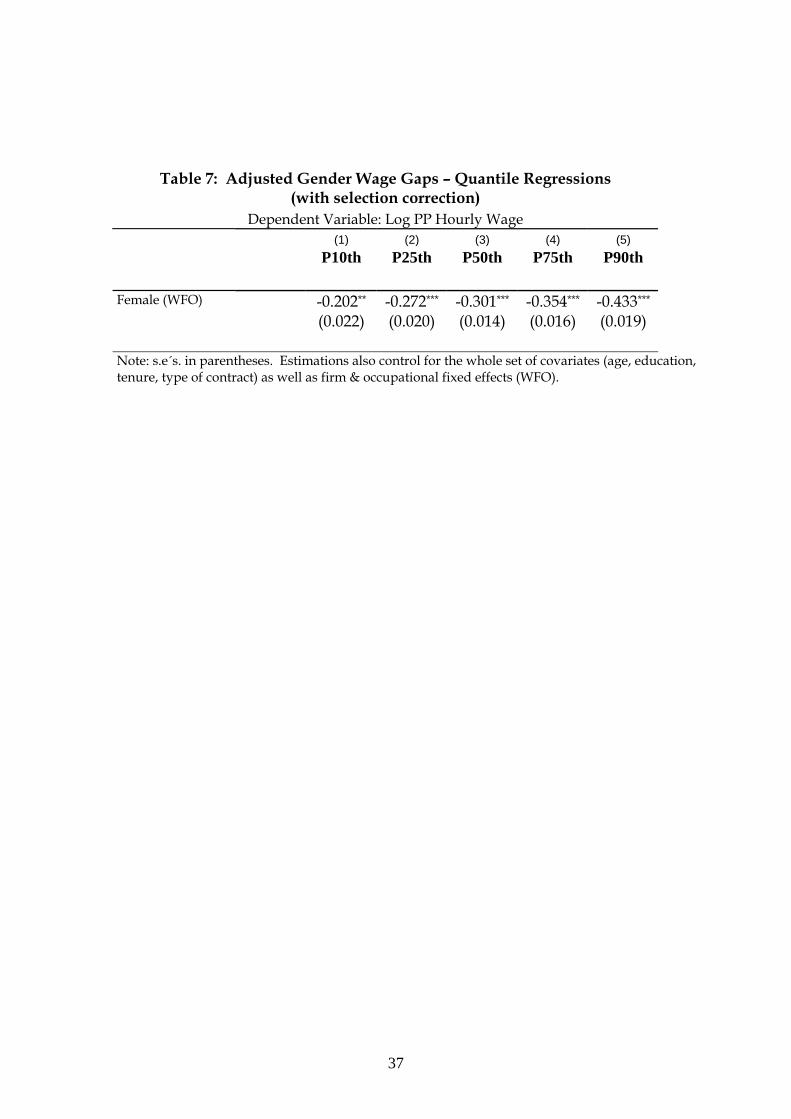
Table 7 reports the QR estimates of the coefficient on the Female dummy for a few

relevant percentiles of the PP distribution. A clear “glass ceiling” pattern emerges with

the gap evolving from 20 log-points at the bottom deciles to 43 log points at the top of

the distribution. In line with our previous discussion, we interpret again this evidence

as yielding higher support to the existence of monopsonistic features in the

determination of PP than to female occupational segregation.

[Table 7 about here]

5. Decomposing the Gender Gap in PP

So far, the estimated models have assumed the same market returns (coefficients) to

male and female characteristics, except the intercept. Since this assumption is rejected

by the data (p=value 0.023), we next report results allowing for different remuneration

to observed characteristics for workers in the PP sample.

Table 8 summarises the results of the slightly modified version of the Oaxaca-Blinder

gender gap decomposition proposed by Gardeazabal and Ugidos (2004) when, as in our

case, there are indicator variables in the hourly wage regressions which can take more

than two categories (e.g.., education and age). The reported results correspond to the

WFO specification. In general, the results indicate that the contribution of differences in

returns to explain the PP gender gap (46 log-points) is much larger (88%) than the

19

contribution of differences in characteristics (12%). Among the former, the largest

components are the differences in constant terms (26 log points) and in the returns to

age. Though we only report the aggregate contribution for all age categories, it is worth

noticing that the two specific categories where differences in returns are larger are the

30-39 and 40-49 groups which jointly account for 5.67 log-points out of the 8.46 log-

points contributed by age. This result somewhat points out that typical ages where

individuals incur in child bearing or other household tasks involves a “marriage

premium “ for males and a “child/elderly parent penalty” for women, in line with

many studies of the gender gap in Spain (see, e.g., de la Rica et al. , 2008). Interestingly,

albeit not large, the differences in returns to tenure favour women, in agreement with

our previous result that firms may find it optimal to offer steeper wage-tenure profiles

to women than to men in order to retain them. Finally, the fact that the female intercept

accounts for 26 log points of the overall gender gap when in the pooled WFO regression

it accounted for 29 log-points may just reflect that the lack of variables in our dataset

capturing civil status and household composition may still biasing upwards the size of

this coefficient.

All in all, the result in this section do not change our previous conjecture that the

gender gap in PP and the corresponding “glass ceiling” may be well due to

monopsonistic features in PP jobs, whereby female lower mobility leads to a rate of

exploitation by firms even when women acquire higher education than men to signal

their commitment to job stability.

6. Concluding remarks

In this paper we have used a large cross-section dataset for Spanish workers in 2006 to

examine whether the gender performance-pay (PP) gap differs from the gender gaps in

other components of wage compensation. We have found evidence that PP responds

more to workers´ performance and that women in PP jobs have several observable

characteristics which are better than men ´s (e.g., educational attainments). Yet, our

main result is that the gender gap in PP is much higher, both in raw terms and adjusted

for observable characteristics, than the gap in non-PP compensation, and that there are

20

clear signs of a “glass ceiling” effect (higher gaps and lower female participation of

women in the upper parts of the PP distribution). Our explanation for these findings

relies mostly on the existence of monopsonistic features in the PP segment of the labour

market, possibly related to women´s lower mobility due to their attachment to

household tasks, and to a lesser extent on theories explaining women ´s segregation in

different occupations than men. Nonetheless, this interpretation has to be taken with a

grain of salt since our dataset lacks information on workers´ civil status and household

composition which can only be (rather imperfectly) proxied by workers´ age groups.

21

References Amuedo-Dorantes, C. & S. de la Rica (2006), “The Role of Segregation and Pay Structure on the

Gender Wage Gap: Evidence from Matched Employer-Employee Data for Spain”, Contributions to Economic Analysis and Policies, Berkeley Electronic Press Journals, 1.

Beaudry, Paul & J. DiNardo (1991), “The effect of implicit contracts on the movement of wages over the business cycle: Evidence from Micro Data”, Journal of Political Economy, 99(4):665-688

Becker, G. (1985), “Human Capital, Effort and the Sexual Division of Labor”, Journal of Labor Economics, 3.

Bertrand, M. & K. Hallock (2001), “The Gender Gap in Top Corporate Jobs”, Industrial and Labor Relations Review,55, 3-21.

Bertrand,M., Goldin, G. & L. F. Katz (2009), “ Dynamics of the gender gap for young professionals in the corporate and financial sectors” NBER W.P. Series 14681.

Booth, A. & J. Frank (1999), “Earnings, Productivity and Performance-Pay”, Journal of Labor Economics, 17 (3).

Booth, A., Francesconi, M & J. Frank (2003), “A sticky floors model of promotion, pay and gender”, European Economic Review, 47, 295-322.

Buchinsky, M.(1998), "Recent Advances in Quantile Regression Models: A Practical Guideline for Empirical Research." Journal of Human Resources , 33.

Card, D. (1996), "The Effect of Unions on the Structure of Wages: A Longitudinal Analysis." Econometrica 64.

Coate, S. & G. Loury (1993), “Will affirmative-action policies eliminate negative stereotypes ”, American Economic Review, 83, 1220-40.

de la Rica, S., Dolado, J.J. & V. Llorens (2008), "Ceilings or floors ?. Gender wage gaps by education in Spain”, Journal of Population Economics, 21, 755-776.

de la Rica, S., Dolado, J.J. & C. García-Peñalosa (2009), "On gender gaps and self-fulfilling expectations: Theory, policies and some empirical evidence", IZA Discussion Paper No. 3553.

DiNardo, J., Fortin, N & T. Lemieux (1996), "Labor Market Institutions and the Distribution of Wages, 1973-1992: A Semiparametric Approach," Econometrica, 64(5), 1001-44.

Dolado, J.J. , J. Jimeno & F. Felgueroso (1997), "Minimum Wages, Collective Bargaining and Wage Dispersion: The Spanish Case" European Economic Review, 41, 713-725 .

Dohmen, T. & A. Falk (2009), “Performance Pay and Multi-dimensional Sorting Productivity, Preferences and Gender”, Forthcoming in American Economic Review.

Ewing, B. (1996), “Wages and performance-based pay: Evidence from NLSY”, Economic Letters 51, 241-246.

Farber, H. & R. Gibbons (1996), “Learning and Wage Dynamics”, The Quarterly Journal of Economics .

22

Gardeázabal, J & A. Ugidos (2004) “ More on identification in detailed wage decompositions”, Review of Economics and Statistics, 86, 1034-36.

Katz, L.F. & K.M. Murphy (1992), “Changes in relative wages, 1963-1987: Supply and demand factors” Quarterly Journal of Economics, 107, 35-78.

Lazear, E. & S. Rosen (1990), “Male and female differentials in job ladders”, Journal of Labor Economics, 8, 106-123.

Lazear, E. (2000): “Performance Pay and Productivity,” American Economic Review, 90(5), 1346–1362.

Lemieux, T. (1998), "Estimating the Effects of Unions on Wage Inequality in a Panel Data Model with Comparative Advantage and Non-Random Selection" Journal of Labor Economics 16, April 1998, pp. 261-291

Lemieux, T. & D. Parent (2009), “Performance Pay and Wage Inequality”, Quarterly Journal of Economics 124(1), 1-49.

Manning, A. (2003), Monopsony in motion: Imperfect competition in Labor Markets, Princeton University Press.

Mincer, J. & S. Polacheck, 1977, “Women´s earnings re-examined”, The Journal of Human Resources, 13 (1).

23

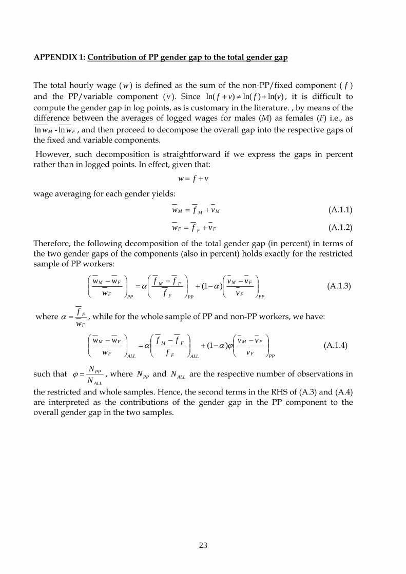
APPENDIX 1: Contribution of PP gender gap to the total gender gap

The total hourly wage ( w ) is defined as the sum of the non-PP/fixed component ( f ) and the PP/variable component ( v ). Since )ln()ln()ln( vfvf +≠+ , it is difficult to compute the gender gap in log points, as is customary in the literature. , by means of the difference between the averages of logged wages for males (M) as females (F) i.e., as

Mwln - Fwln , and then proceed to decompose the overall gap into the respective gaps of the fixed and variable components.

However, such decomposition is straightforward if we express the gaps in percent rather than in logged points. In effect, given that:

vfw +=

wage averaging for each gender yields:

MMM vfw += (A.1.1)

FFF vfw += (A.1.2)

Therefore, the following decomposition of the total gender gap (in percent) in terms of the two gender gaps of the components (also in percent) holds exactly for the restricted sample of PP workers:

PPF

FM

PPF

FM

PPF

FM

vvv

fff

www

⎟⎟⎠

⎞⎜⎜⎝

⎛ −−+⎟⎟

⎠

⎞⎜⎜⎝

⎛ −=⎟⎟

⎠

⎞⎜⎜⎝

⎛ − )1( αα (A.1.3)

where F

F

wf

=α , while for the whole sample of PP and non-PP workers, we have:

PPF

FM

ALLF

FM

ALLF

FM

vvv

fff

www

⎟⎟⎠

⎞⎜⎜⎝

⎛ −−+⎟⎟

⎠

⎞⎜⎜⎝

⎛ −=⎟⎟

⎠

⎞⎜⎜⎝

⎛ − ϕαα )1( (A.1.4)

such that ALL

PP

NN

=ϕ , where PPN and ALLN are the respective number of observations in

the restricted and whole samples. Hence, the second terms in the RHS of (A.3) and (A.4) are interpreted as the contributions of the gender gap in the PP component to the overall gender gap in the two samples.

24

APPENDIX 2: An illustrative model of the gender implications of PP

(A) Competitive wages

Let us assume that a PP worker of (exogenous) skill δ receives a wage W per unit of output produced and that firms incur a fixed C of monitoring the worker which in a competitive market is paid by the worker. Denoting effort by e , output is assumed to be )( e+δ . Effort produces a disutility cost )(ec which is increasing and convex. We assume the functional form )1/()( 1 γγ += +eec with

0>γ . Given women ´s higher involvement in housework, their disutility of effort is higher than for men, namely, )1/(1 γφ γ ++e , where φ >1. Therefore, we can write down the utility of men (M) and women (F) in PP jobs as follows:

)1/()( 1 γδ γ +−−+= +eCeWU PPM (A.2.1)

)1/()( 1 γφδ γ +−−+= +eCeWU PPF (A.2.2)

Regarding non PP jobs, let us assume that the worker produces a minimum level of output, say δ , which can be monitored by the firm at no cost and does not involve any effort. After all, it is painful to produce output and, in the absence of monitoring, the worker can get away without producing any more than δ . This implies that the utility for both men and women of this type of job is simply given by:

δWU NPP = (A.2.3)

Workers´ effort decision in PP jobs is simply obtained by equating the marginal revenue from exerting effort to its marginal cost. From (A.2.1) and (A.2.2), it yields γ*

MeW = and γφ *FeW = , whereby γγγ φ FFM eee *** >= . Substituting

these two expression into (A.2.1) and (A.2.2), implies that worker FMi ,(= ) will choose PP for ,*

iδδ > where

NPPFMFMMMM

PPM UWCeeeeU ==−+

+=+

+= ++ δϕδ

γγφδ

γγδ γγγγ *1*1*

11)( (A.2.4)

NPPFFFF

PPF UWCeeU ==−+

+= + δδ

γγφδ γγ *1*

1)( (A.2.5)

Comparing both expressions, we get that MMFF δφδδ >= ** . Thus, assuming that the skills distribution is identical across genders, we should expect fewer women in PP jobs and, conditionally on receiving PP, higher ability among female workers than among male workers.

Further, if women are aware of discrimination in non- PP jobs where, say, they get paid δαWU NPP

F = , with 10 <<α , whereas δWU NPPM = , then obviously

they will have higher preference for PP jobs than before. Moreover, in this case they will even be more prominent in PP jobs than men if 1=φ .

25

(B) Predetermined wages and job attachment uncertainty

A slightly different model where wages are no longer given but set by employers in order to avoid career interruption can be written using a slight adaptation of Lazear and Rosen ´s (1992) model of assignment of workers to slow and fast- jobs. Let us assume that individuals in PP jobs work for two periods and are endowed with the same ability δ which is known to the firm. In the initial period, they produce δ and receive a wage W1. As a result of longer tenure, their productivity in period 2 raises toµδ , where 1>µ and get paid W2. It is assumed that, workers receive a disutility shock, ω, in both periods which may force them to quit the job (say, for family duties). The ω shock is an i.i.d. random variable, independent across periods, with c.d.f. F(ω) which is revealed to the worker after the wage in either period has been set by the firm. Thus, wages are predetermined and workers will stay in the firm both periods as long as Wti - ω ≥ 0, t=1, 2 and i=F, M .

The key difference between men and women is that the c.d.f. for men, FM(ω), is stochastically dominated by the c.d.f. for women FF(ω), namely FM(ω) > FF(ω) for ω > 0. This assumption captures the fact that women are more likely to be affected by the shock than men. To simplify matters, and without loss of generality in terms of the qualitative results, we will assume that dF(.) are uniform distributions, such that the density functions verify: fM(ω) = U[0, εM] and fF(ω) = U[0, εF ], with εF > εM.

To solve for both wages, we proceed backwards in time. Under the assumption that the wage in period 2, W2i (i=f, m), is offered before ω is realized, employers will choose W2i in order to maximize expected profits in period 2, subject to the participation constraint in this period and conditional on the probability of staying in the firm during period 1 (equal to iiW ε/1 under a uniform distribution), namely:

( ) FMiWWWdWWii

i

i

W

W

ii

i

W i

i

i

,,][maxmax 2222

10 2

1

2

2

2

=−=−∫ µδε

ωµδε

(A.2.6)

whereby the first-order condition (f.o.c.) w.r.t. W2i implies that the wage paid in

equilibrium to male and female workers is identical:11

W2* = 2/µδ (A.2.7)

and by replacing W2* into the bracketed term in (A.2.6) , the firm ´s profit in period 2 (Π*2i) is given by Π*2i = 222

1 4/)( iiW εµδ .

Going back to period 1, firms will choose W1i to maximize the sum of expected profits in both periods, subject to the participation constraint in that period, i.e.

11 This is just the average of the worker´ s productivity´ and the outside wage which is assumed to be zero. The weight ½ in the average is due to the choice of the uniform distribution in the illustration. Alternative distributions will give rise to a weighted average with unequal weights.

26

( ) FMiW

dWi

iW

ii

W

i

i

,},)(4

1{max 22

21

0 11

1

=+−∫ µδε

ωδε

(A.2.7)

which implies that:

i

iWε

µδδ8

)(2

2*

1 += (A.2.8)

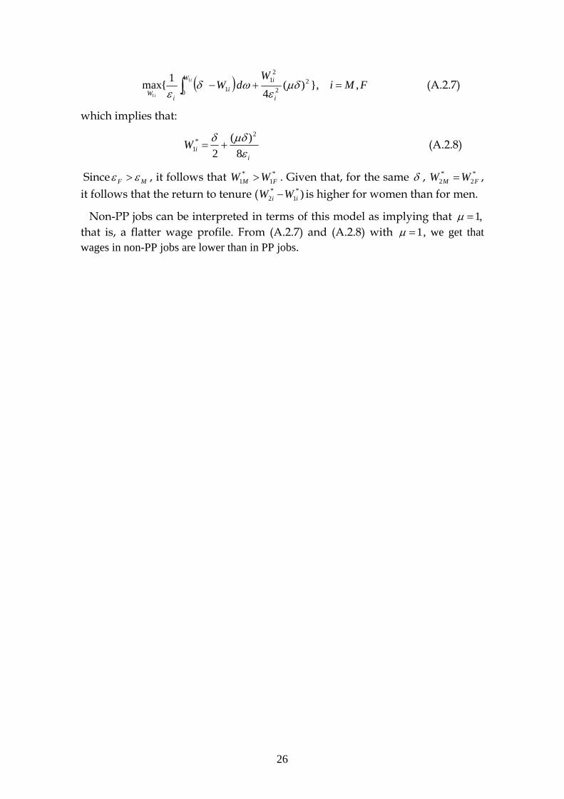
Since MF εε > , it follows that *1

*1 FM WW > . Given that, for the same δ , *

2*

2 FM WW = , it follows that the return to tenure ( )*

1*

2 ii WW − is higher for women than for men.

Non-PP jobs can be interpreted in terms of this model as implying that ,1=µ that is, a flatter wage profile. From (A.2.7) and (A.2.8) with 1=µ , we get that wages in non-PP jobs are lower than in PP jobs.

27

Figure 1. Gender wage gaps (Total, Non-PP and PP components) - Whole Sample (in percent)-

Figure 2. Gender wage gaps and the contribution of PP component - Sample of PP workers (in percent)-

0%5%

10%15%20%25%30%35%40%45%50%

p_0_10 p_10_25 p_25_50 p_50_75 p_75_90 p_90_100

f contribution v gap w

28

Table 1 – Sample characteristics (Full-time workers between 18-65 years) Variables Women (65,233) Men (129,930)

Mean Mean

Individual Characteristics Education

Primary or less 0.176 0.275 Secondary 0.508 0.545 University 0.316 0.180 Age Less 30 years 0.257 0.200 31-40 0.354 0.323 41-50 0.245 0.265 >50 0.143 0.212 Tenure (years) 7.410 8.867 Permanent Contract 0.727 0.768 Wages Total Hourly Wage (logs) 2.185 2.391 Performance Pay % PP job 0.227 0.227 Total Hourly PP (only PP workers) 1.127 1.958 Firm Characteristics Size <50 workers 0.339 0.403 51-200 workers 0.265 0.288 >200 workers 0.396 0.309 Firm Bargaining Agreement. 0.163 0.194 Exporting firms 0.163 0.194

Source: EES (2006)

29

Table 2a: Characteristics of workers and firms by type of job and gender

PP Jobs

Non-PP Jobs

Women Men Women Men (14789 obs.) (29460 obs.) (50444 obs.) (100470 obs.)

Variables Mean Mean Mean Mean Education Primary or less 0.107 0.178 0.196 0.304 Secondary 0.494 0.545 0.512 0.545 University 0.399 0.277 0.292 0.151 Age Less 30 years 0.204 0.149 0.273 0.215 31-40 0.381 0.313 0.346 0.325 41-50 0.265 0.294 0.239 0.257 >50 0.150 0.244 0.141 0.203 Tenure (years) 9.281 12.037 6.861 7.938 Indefinite Contract 0.814 0.862 0.741 0.741 Firm Characteristics Size <50 workers 0.201 0.235 0.380 0.452 51-200 workers 0.239 0.297 0.272 0.285 >200 workers 0.560 0.467 0.348 0.262 Collective Bargaining(ref: Industry level)

Firm Bargaining Agr. 0.193 0.288 0.154 0.167

Firm Market (ref: non-exp .firms) Exporting firms

0.231

0.261

0.135

0.153

30

Table 2b: Incidence of PP by industry and occupation

Mean Std. Dev. No. Obs.

Industries Mine & Extractive Ind. 0.188 0.391 2919 Manufactures 0.205 0.404 74332 Energy 0.324 0.468 4627 Construction 0.127 0.333 17096 Retail trade 0.241 0.427 17131 Hotels and Restaurants 0.123 0.328 8315 Transportation 0.324 0.468 12710 Financial Intermediation 0.598 0.490 10475 Real State and Res. Serv. 0.194 0.395 16342 Education 0.092 0.289 7998 Health 0.287 0.452 14178 Other Services 0.146 0.353 9040 Occupations Managers 0.497 0.500 6190 Professionals 0.288 0.453 20295 Technicians 0.326 0.469 30184 Clerks 0.257 0.437 24761 Personal Services 0.196 0.397 17528 Agriculture and Fisheries 0.146 0.353 542 Craftsmen 0.169 0.375 37918 Operators and Assemblers 0.180 0.384 34822

Laborers, non-qualified operators 0.127 0.333 22923

31

Table 2c: Share of women throughout PP distribution

% Women in percentile

[p0-p10] 40.6% [p11-pw25] 40.3% [p26-pw50] 39.5% [p51-pw75] 32.0% [p76-pw90] 24.8% [p91-pw95] 18.6% [p95-pw100] 15.9%

Table 3a: Hourly Wages in PP and Non-PP Jobs  

  Pay Performance Jobs  Non-Performance Pay Jobs   

  Women  Men  Women  Men   

Ratio  Ratio      Total Hourly

Wage(€) PP/Total

Wage (%)

Total Hourly

Wage(€) PP/Total Wage(%) 

Total Hourly

Wage(€) 

Total Hourly

Wage(€)   

Average  14.503  7.164  19.144  9.012  9.678  11.665   P10th  6.060  0.976  7.801  0.009  3.721  4.689   P25th  8.577  2.087  10.804  0.025  5.884  7.308   P50th  12.479  4.657  16.051  0.060  8.126  9.826   P75th  18.800  9.491  23.546  0.127  12.048  14.192   P90th  24.842  16.684  33.127  0.217  17.795  20.162   

32

Table 3b: Hourly wage components in PP Jobs (in €)

Women Men

PP wage

Other wage components PP

wage Other wage components

Average 1.127 13.376 1.958 17.186

P10th 0.102 5.648 0.132 7.031 P25th 0.225 7.850 0.324 9.675 P50th 0.539 11.679 0.890 14.758 P75th 1.311 17.509 2.198 21.694 P90th 2.594 22.828 4.493 29.597

33

Table 4: Log hourly wage regressions  

Dependent Variable: Log Hourly Total Wage (1) (2) (3)  

PP Workers  Non-PP Workers Pooled 

0.208*** PP Job  (0.009)

-0.223*** -0.212*** -0.219*** Female (0.004) (0.003) (0.004) 0.139*** 0.098*** 0.095*** Age 30-39 (ref:<30) (0.006) (0.003) (0.004) 0.199*** 0.116*** 0.114*** Age 41-49 (0.007) (0.004) (0.004) 0.227*** 0.161*** 0.161*** Age 50-59 (0.008) (0.004) (0.005) 0.262*** 0.155*** 0.158*** Age >60 (0.014) (0.007) (0.008) 0.277*** 0.223*** 0.215*** College (ref: Primary) (0.007) (0.005) (0.004) 0.077*** 0.063*** 0.060*** Secondary (0.006) (0.003) (0.003) 0.044*** 0.042*** 0.043*** Tenure (0.001) (0.000) (0.000)

-0.001*** -0.001*** -0.001*** Tenure sq. (0.000) (0.000) (0.000) 0.282*** 0.313*** 0.312*** Permanent Contract (0.006) (0.003) (0.003)

Firm Size: 50-199  0.067*** 0.095*** 0.094*** Ref: <50)  (0.005) (0.003) (0.003)

0.118*** 0.166*** 0.164*** Firm Size: >199 (0.005) (0.003) (0.003) 0.011 0.015* 0.013* Firm Agreement 

(0.008) (0.008) (0.007) 0.027*** 0.035*** 0.045*** Export market (0.005) (0.003) (0.003)

Interactions with PP           -0.007 Female*PP    (0.005)   -0.047*** Age 30-39*PP

(ref:<30)    (0.007)   -0.029*** Age 41-49*PP    (0.008)   0.072*** Age 50-59*PP    (0.010)

34

  0.101*** Age >60*PP    (0.016)   0.089*** College*PP (ref:

Primary)    (0.007)   0.030*** Secondary*PP    (0.006)

 

0.011*** (0.004)

-0.025***

Tenure*PP Permanent Contract*PP    (0.007) Firm Size: (ref<50) 50-199*PP    -0.027***     (0.006)

  -0.042*** Firm Size: >199*PP    (0.006)   -0.006** Firm Agreement*PP    (0.003)

Export. Firm *PP    -0.014***     (0.006) No. Observations  44249 150914 195163 R sq. 0.605 0.511 0.573

Note: S.e´s. in parentheses. Estimations also control for industry dummies (11) and occupational dummies (8).  

35

Table 5: Probit estimation

Dependent Variable: Receiving Performance Pay (1/0)

(1) (2)

-0.047*** -0.103*** Female (0.008) (0.016) 0.052*** 0.016** Age 30-39 (ref:<30) (0.010) (0.008) 0.032*** 0.002 Age 41-49 (0.011) (0.013) 0.015 -0.010 Age 50-59

(0.013) (0.015) -0.076*** -0.099*** Age >60 (0.023) (0.026) 0.260*** 0.262*** University (ref: Primary) (0.013) (0.013) 0.164*** 0.161*** Secondary (0.009) (0.009) 0.030*** 0.031*** Tenure (0.001) (0.001)

-0.001*** -0.001*** Tenure square (0.000) (0.000) 0.037*** 0.035*** Permanent Contract (0.010) (0.010)

Firm Size: 50-199 0.295*** 0.301*** Ref: <50) (0.009) (0.009)

0.485*** 0.478*** Firm Size: >199 (0.008) (0.009) 0.096** 0.120*** Firm Collective Agreement (0.009) (0.009) 0.122*** 0.120*** Exporting firm (0.009) (0.011)

Interactions with female

-0.047*** Age 30-39*Female (ref:<30) (0.019) -0.031*** Age 41-49*Female (0.011) 0.072*** Age 50-59*Female (0.024) 0.062 Age >60*Female (0.052)

No. Observations 195163 195163 Pseudo R2 0.111 0.123

36

(1) (2) (3) (4) (5)

OLS Heckman selection

Within Firm

Within Occupations

Within Firm-

Occupation -0.407*** -0.453*** -0.343*** -0.434*** -0.290*** Female (0.014) (0.018) (0.011) (0.019) (0.011) 0.257*** 0.337*** 0.181*** 0.281*** 0.143*** Age 30-39 (ref:<30) (0.019) (0.024) (0.018) (0.024) (0.017) 0.334*** 0.381*** 0.252*** 0.313*** 0.192*** Age 41-49 (0.022) (0.026) (0.019) (0.027) (0.019) 0.326*** 0.353*** 0.238*** 0.298*** 0.184*** Age 50-59 (0.026) (0.031) (0.022) (0.031) (0.021) 0.601*** 0.532*** 0.416*** 0.395*** 0.311*** Age >60 (0.044) (0.052) (0.037) (0.053) (0.036) 0.793*** 0.350*** 0.362*** 0.636*** 0.280*** College (ref: Primary) (0.020) (0.064) (0.128) (0.053) (0.062) 0.109*** 0.380*** 0.010** 0.213*** 0.043 Secondary (0.018) (0.035) (0.064) (0.029) (0.035)

0.023***

0.061***

0.019***

0.060***

0.0173***

Tenure (0.002) (0.005) (0.005) (0.005) (0.006)

-0.001*** -0.001*** -0.001*** -0.001*** -0.000*** Tenure square (0.000) (0.000) (0.000) (0.000) (0.000) 0.450*** 0.534*** 0.389*** 0.443*** 0.362*** Permanent Contract (0.020) (0.024) (0.021) (0.024) (0.021)

Firm Size: 50-199 -0.126*** 0.236*** 0.317*** Ref: <50) (0.018) (0.045) (0.048)

-0.209*** 0.366*** 0.505*** Firm Size: >199 (0.017) (0.068) (0.0726)

-0.019 Firm Agreement (0.016)

Exporting firm 0.114*** 0.262*** 0.263*** (0.016) (0.024) (0.023) Inv. Mills Ratio 1.628*** 1.693*** 1.984*** 1.513 *** (0.170) (0.198) (0.141) 0.474) No. Obs. 44249 195163 44249 44249 44249 R sq. 0.186 0.175 0.115 0.089 0.125

Table 6: Estimates of alternative specifications of log hourly wage equation corrected for selectivity

Dependent Variable: log PP wage component

37

Table 7: Adjusted Gender Wage Gaps – Quantile Regressions (with selection correction)

Dependent Variable: Log PP Hourly Wage (1) (2) (3) (4) (5) P10th P25th P50th P75th P90th

-0.202**

(0.022) -0.272***

(0.020) -0.301***

(0.014) -0.354***

(0.016) -0.433***

(0.019)

Female (WFO)

Note: s.e´s. in parentheses. Estimations also control for the whole set of covariates (age, education, tenure, type of contract) as well as firm & occupational fixed effects (WFO).

38

Table 8: Oaxaca Decomposition of (log) hourly Gap in PP

Unadjusted Gender Wage Gap in PP: 46 log-points

Variables

Absolute [relative] Contribution of Diff.

in Characteristics (Xm-Xf)*βm

Absolute [relative] Contribution of Diff.

in Returns (βm-βf)*Xf

Sample Selection 0.62 [1.34%]

-1.56 [-3.39%]

Tenure 3.44 [7.47%]

-1.93 [-4.19%]

Education -2.82 [-6.13%]

3.83 [8.33%]

Age 1.35 [2.93%]

8.46 [18.39%]

Type of Contract 1.02 [2.22%]

2.42 [5.26%]

Occup. and Firm Effects

1.81 [3.93%]

3.36 [7.30%]

Constant 26.0 [56.52%]

Total 5.42 [11.8%]

40.58 [88.2%]

Note: Decomposition based on WFO estimation for men and women allowing for different returns by gender.