Embed Size (px)
Citation preview

SANDIA REPORTSAND2014-18590Unlimited ReleasePrinted September 2014
Peridynamic Model for FatigueCracking
Stewart A. Silling
Abe Askari
Prepared bySandia National LaboratoriesAlbuquerque, New Mexico 87185 and Livermore, California 94550
Sandia National Laboratories is a multi-program laboratory managed and operated by Sandia Corporation,a wholly owned subsidiary of Lockheed Martin Corporation, for the U.S. Department of Energy’sNational Nuclear Security Administration under contract DE-AC04-94AL85000.
Approved for public release; further dissemination unlimited.

Issued by Sandia National Laboratories, operated for the United States Department of Energyby Sandia Corporation.
NOTICE: This report was prepared as an account of work sponsored by an agency of the UnitedStates Government. Neither the United States Government, nor any agency thereof, nor anyof their employees, nor any of their contractors, subcontractors, or their employees, make anywarranty, express or implied, or assume any legal liability or responsibility for the accuracy,completeness, or usefulness of any information, apparatus, product, or process disclosed, or rep-resent that its use would not infringe privately owned rights. Reference herein to any specificcommercial product, process, or service by trade name, trademark, manufacturer, or otherwise,does not necessarily constitute or imply its endorsement, recommendation, or favoring by theUnited States Government, any agency thereof, or any of their contractors or subcontractors.The views and opinions expressed herein do not necessarily state or reflect those of the UnitedStates Government, any agency thereof, or any of their contractors.
Printed in the United States of America. This report has been reproduced directly from the bestavailable copy.
Available to DOE and DOE contractors fromU.S. Department of EnergyOffice of Scientific and Technical InformationP.O. Box 62Oak Ridge, TN 37831
Telephone: (865) 576-8401Facsimile: (865) 576-5728E-Mail: [email protected] ordering: http://www.osti.gov/bridge
Available to the public fromU.S. Department of CommerceNational Technical Information Service5285 Port Royal RdSpringfield, VA 22161
Telephone: (800) 553-6847Facsimile: (703) 605-6900E-Mail: [email protected] ordering: http://www.ntis.gov/help/ordermethods.asp?loc=7-4-0#online
DE
PA
RT
MENT OF EN
ER
GY
• • UN
IT
ED
STATES OFA
M
ER
IC
A
2

SAND2014-18590Unlimited Release
Printed September 2014
Peridynamic Model for Fatigue Cracking
Stewart A. SillingMultiscale Science DepartmentSandia National LaboratoriesAlbuquerque, NM 87185-1322
Abe AskariPropulsion System Engineering
The Boeing CompanySeattle, WA
Abstract
The peridynamic theory is an extension of traditional solid mechanics in which thefield equations can be applied on discontinuities, such as growing cracks. This paperproposes a bond damage model within peridynamics to treat the nucleation and growthof cracks due to cyclic loading. Bond damage occurs according to the evolution of avariable called the “remaining life” of each bond that changes over time according tothe cyclic strain in the bond. It is shown that the model reproduces the main featuresof S-N data for typical materials and also reproduces the Paris law for fatigue crackgrowth. Extensions of the model account for the effects of loading spectrum, fatiguelimit, and variable load ratio. A three-dimensional example illustrates the nucleationand growth of a helical fatigue crack in the torsion of an aluminum alloy rod.
3

Acknowledgment
This work was sponsored by The Boeing Company through CRADA No. SC02/01651.
4

Contents
1 Introduction . . . . . . . . . . . . . . . . . . . . . . . . . . . . . . . . . . . . . . . . . . . . . . . . . . . . . . . . . . . . . . . . . . . . . 72 Summary of the peridynamic theory . . . . . . . . . . . . . . . . . . . . . . . . . . . . . . . . . . . . . . . . . . . . . . 93 Structure of a crack tip deformation field . . . . . . . . . . . . . . . . . . . . . . . . . . . . . . . . . . . . . . . . . 134 Fatigue model . . . . . . . . . . . . . . . . . . . . . . . . . . . . . . . . . . . . . . . . . . . . . . . . . . . . . . . . . . . . . . . . . . . . 16
4.1 Phase I: Nucleation . . . . . . . . . . . . . . . . . . . . . . . . . . . . . . . . . . . . . . . . . . . . . . . 174.2 Phase II: Crack growth . . . . . . . . . . . . . . . . . . . . . . . . . . . . . . . . . . . . . . . . . . . . 174.3 Scaling of parameters with the horizon . . . . . . . . . . . . . . . . . . . . . . . . . . . . . . . . 204.4 Transition from phase I to phase II . . . . . . . . . . . . . . . . . . . . . . . . . . . . . . . . . . . 22
5 Examples . . . . . . . . . . . . . . . . . . . . . . . . . . . . . . . . . . . . . . . . . . . . . . . . . . . . . . . . . . . . . . . . . . . . . . . . 235.1 Nucleation at a stress concentration . . . . . . . . . . . . . . . . . . . . . . . . . . . . . . . . . . 245.2 Crack growth in a compact test specimen . . . . . . . . . . . . . . . . . . . . . . . . . . . . . 245.3 Torsion of a rod . . . . . . . . . . . . . . . . . . . . . . . . . . . . . . . . . . . . . . . . . . . . . . . . . . 28
6 Extensions . . . . . . . . . . . . . . . . . . . . . . . . . . . . . . . . . . . . . . . . . . . . . . . . . . . . . . . . . . . . . . . . . . . . . . . 336.1 Loading spectrum . . . . . . . . . . . . . . . . . . . . . . . . . . . . . . . . . . . . . . . . . . . . . . . . . 336.2 Fatigue limit . . . . . . . . . . . . . . . . . . . . . . . . . . . . . . . . . . . . . . . . . . . . . . . . . . . . . 346.3 Phase III . . . . . . . . . . . . . . . . . . . . . . . . . . . . . . . . . . . . . . . . . . . . . . . . . . . . . . . . 346.4 Nonzero load ratio . . . . . . . . . . . . . . . . . . . . . . . . . . . . . . . . . . . . . . . . . . . . . . . . 34
7 Discussion. . . . . . . . . . . . . . . . . . . . . . . . . . . . . . . . . . . . . . . . . . . . . . . . . . . . . . . . . . . . . . . . . . . . . . . . 36
Figures
1 Crack growth in a peridynamic solid is determined by damage to bonds inmany directions. . . . . . . . . . . . . . . . . . . . . . . . . . . . . . . . . . . . . . . . . . . . . . . . . . . 12
2 Schematic of bonds near a crack tip. The core bond has the largest strain.Only bonds oriented normal to the crack are shown. . . . . . . . . . . . . . . . . . . . . . 13
3 Bond strain ahead of a crack for three peridynamic (PD) models with varyinghorizon δ. All three approach the LEFM solution as distance from the cracktip increases. . . . . . . . . . . . . . . . . . . . . . . . . . . . . . . . . . . . . . . . . . . . . . . . . . . . . . 15
4 Loading cycles N1 as a function of bond strain ε1 for nucleation of damage . . 185 A bond ξ near an approaching fatigue crack undergoes cyclic strain ε, which
changes over time, eventually causing the bond to break. . . . . . . . . . . . . . . . . . 216 Geometry of the hourglass test specimen modeled in Example 1 (all dimen-
sions are in mm). . . . . . . . . . . . . . . . . . . . . . . . . . . . . . . . . . . . . . . . . . . . . . . . . . 257 Left: nucleation of fatigue damage in the hourglass test specimen modeled in
Example 1. Right: nucleation quickly leads to growth of a crack through thespecimen. . . . . . . . . . . . . . . . . . . . . . . . . . . . . . . . . . . . . . . . . . . . . . . . . . . . . . . . 26
8 Strain amplitude as a function of loading cycle at which nucleation of damageoccurs in the hourglass test specimen modeled in Example 1. Model resultsare shown with and without a fatigue limit. Experimental data from Zhaoand Jiang [35]. . . . . . . . . . . . . . . . . . . . . . . . . . . . . . . . . . . . . . . . . . . . . . . . . . . . 27
5

9 Geometry of the compact test specimen modeled in Example 2 (all dimensionsare in mm). . . . . . . . . . . . . . . . . . . . . . . . . . . . . . . . . . . . . . . . . . . . . . . . . . . . . . . 28
10 Model results for crack growth in the compact test specimen in Example 2.Left: 0 cycles. Right: 89,000 cycles. Displacements are exaggerated x50.Colors indicate vertical displacement. . . . . . . . . . . . . . . . . . . . . . . . . . . . . . . . . . 29
11 Compact test specimen model results for R = 0.1 (Example 3). Left: crackgrowth distance as a function of loading cycle. Right: Paris law plot, includingtest data [36]. . . . . . . . . . . . . . . . . . . . . . . . . . . . . . . . . . . . . . . . . . . . . . . . . . . . . 30
12 Geometry of the rod modeled in Example 3 (all dimensions are in mm). . . . . . 3113 Computed solution for the torsion example problem after 3.5 × 10⁷ cycles.
The two views are from opposite sides of the specimen. The white dot showsthe location of the initial cavity. Shading indicates magnitude of displacement. 32
6

1 Introduction
The ability to understand the process of fatigue cracking in complex structures and het-erogeneous materials depends on the ability to model damage nucleation and the growth ofcurved, three-dimensional cracks under general loading conditions. The peridynamic model[26], by virtue of treating discontinuities with the same mathematical equations as pointswhere the deformation is continuous, potentially avoids some of the difficulties of traditionalcomputational methods in treating complex patterns of fatigue crack growth. Because peri-dynamics does not assume a pre-existing crack, it also potentially offers a way to model thenucleation and growth phases of damage consistently. This paper presents an attempt toapply the peridynamic approach to the nucleation and growth of fatigue cracks.
Most modern continuum treatments of the growth of a crack under cyclic loading arederived from the Paris law [21]. Various corrections have been proposed for this law, whileretaining the basic idea that the cyclic change in stress concentration factor at the crack tipis the driving force, as discussed by Pugno et al. [22] and the references contained therein.A review of earlier theories is provided by Erdogan [7].
In engineering, analysis of resistance of structures to fatigue largely relies on the extrap-olation of empirical data derived from geometrically simple specimens to the more complexcyclic stress field that the structure experiences. The empirical data are usually based oncyclic uniaxial states of stress compiled into S-N or ε-N curves. By applying these curves tostress states in structures with suitable corrections for stress concentrations due to notchesand other factors, engineers can reliably design against fatigue failure (see, for example,[3]). A number of computational tools are available to apply this type of methodology tomechanical design (for example, MSC Fatigue [17]).
Other computational approaches to fatigue crack growth include that of McClung andSehitoglu [12, 13], who used a node release method to advance the crack in a two-dimensionalmodel and investigated the importance of mesh refinement ahead of the crack. Moes,Gravouil, and Belytschko [15, 16] and Sukumar, Chopp, and Moran [34] applied XFEMto three-dimensional fatigue crack growth. Bordas and Moran [2] describe modeling of fa-tigue in complex structures, using the standard Paris law, in an enriched element formulationin the EDS-PLM/I-DEAS commercial finite element code. Shi et al. and Shi, Chopp, Lua,Sukumar, and Belytschko [25, 24] implemented a fatigue model using XFEM in Abaqus usinga modified Paris law expression. De-Adres, Perez, and Ortiz [4] and Nguyen, Repetto, Ortiz,and Radovitzky [18] applied a cohesive element approach to fatigue crack growth, includingshort cracks and the effect of overload, in two dimensions. Much effort has been devotedto investigating the role of crack closure in fatigue crack growth in metals [6]; see [23] for arecent summary.
In spite of the century-old history of research on fatigue and the valuable software toolsthat are available to the engineer, fatigue has not been treated as a full participant withinthe scope continuum mechanical theory. The available models for fatigue crack nucleation (aterm we use synonymously with initiation) apply some supplemental criterion that “watches”
7

a stress field that is computed under the assumption of continuous deformation, but is essen-tially a bystander in the actual computation. There has previously no way to treat the actualprocess of the emergence of a discontinuity due to cyclic loading within the field equationsof continuum mechanics. This is not surprising, due to the well-known inapplicability of thepartial differential equations of continuum mechanics on an evolving discontinuity.
The peridynamic equations, because they do not involve partial derivatives of the defor-mation with respect to the spatial coordinates, potentially offer a way to treat the detailsof fatigue crack nucleation and growth as part of a consistent mathematical description of aboundary value problem, without supplemental relations dictating crack growth. The ma-terial model, if a suitable damage law can be specified, results in accumulation of damageleading to the possible emergence of discontinuities such as cracks. The purpose of thepresent work is to propose and demonstrate such a material model.
8

2 Summary of the peridynamic theory
The peridynamic theory is an extension of the standard mathematical theory of solid me-chanics that is compatible with the discontinuous nature of cracks. In contrast to the PDEsof the standard theory, which cannot be applied directly on a growing crack, the peridy-namic theory uses integro-differential equations that do not involve the spatial derivativesof the deformation. The field equations therefore apply on a crack. The peridynamic modelwas introduced in the year 2000 [26] and has undergone extensive expansion and improve-ment since then. The review article [31] and the book by Madenci and Oterkus [10] containup-to-date summaries of the theory.
The equation of motion in the peridynamic model takes the form
ρ(x)y(x, t) =
∫Hx
f(x′,x, t) dVx′ + b(x, t), ∀x ∈ B, t ≥ 0 (1)
where y is the deformation map, x is a material point in the reference configuration of abody B, ρ is the density field, and b is the prescribed external body force density. Thespherical neighborhood Hx ⊂ B centered at x, but excluding x, is called the family of x:
Hx ={x′ ∈ B
∣∣ 0 < |x′ − x| ≤ δ}.
The radius of the neighborhood δ is called the horizon, which may be finite or infinite andmay be thought of as a material property. The vector field f is the pairwise bond force density,which depends on the deformation through the constitutive model. Since the integral in (1)sums up forces on x from all of its neighbors, the peridynamic model can be thought of asa “continuum version of molecular dynamics.”
The vector in the reference configuration defined by
ξ = x′ − x, x′ ∈ Hx
is called a bond. The constitutive model in the peridynamic theory prescribes the pairwiseforce density f in each bond. This pairwise force density consists of two parts that aredetermined by application of the constitutive model at x and x′:
f(x′,x, t) = t(x′,x, t)− t(x,x′, t)
where the two terms on the right hand side contain the contributions from Hx and Hx′
respectively. To express the contribution from the deformation of Hx, we write
t(x′,x, t) = T[x]〈x′ − x〉
where T[x] is a function called the force state at x that maps any bond x′ − x to the corre-sponding force density vector in the bond. The force state is an example of a peridynamicstate, which is simply a function defined on a family.
9

The basic kinematical quantity for purposes of constitutive modeling is the deformationstate, whose value for any bond is the deformed image of the bond:
Y[x]〈x′ − x〉 = y(x′, t)− y(x, t).
A constitutive model T is a state-valued function of a state:
T = T(Y).
The structure of such a constitutitive model is analogous to a tensor valued function of atensor in the standard theory, that is, σ = σ(F), where F = ∂y/∂x.
A constitutively linear elastic isotropic solid may be modeled as follows. For a given bondξ, define the bond direction by
M〈ξ〉 =ξ
|ξ|.
Let ω be a weighting function defined on the family, and let a normalization constant m bedefined by
m =
∫Hω〈ξ〉|ξ|2 dVξ.
For any deformation state Y, define the extension state by
e〈ξ〉 = |Y〈ξ〉| − |ξ| (2)
which represents the change in length of the bond ξ under the deformation. Let the nonlocaldilatation be defined by
θ =3
m
∫Hω〈ξ〉|ξ| e〈ξ〉 dVξ.
This nonlocal dilatation has the same value as the dilatation in the standard (local) theory(that is, θ =Tr ε, where ε is the linearized strain tensor) for small, homogeneous deformationsof a body. Let k be the bulk modulus and let µ be the shear modulus for the isotropic elasticsolid. Then the force state is given by
T〈ξ〉 =ω〈ξ〉M〈ξ〉
m
[3kθ|ξ|+ 15µ
(e〈ξ〉 − θ|ξ|
3
)]. (3)
The quantity that multiplies 15µ in this expression represents the deviatoric part of thedeformation, that is, the extension state after the volume change is subtracted off. See [30]for further details of this model, which is called the linear peridynamic solid (LPS) model.Unfortunately, this name is slightly misleading because, unlike a constitutive model in thefully linearized peridynamic theory [27], the LPS model uses nonlinear kinematics (as maybe seen in (2)).
Damage in peridynamics is usually modeled by irreversible bond breakage. After a bondbreaks according to some criterion, it no longer sustains any force density. Many types of
10

bond breakage criteria are available. The simplest criterion is that a bond ξ breaks when itsbond strain, defined by
s =e〈ξ〉|ξ|
exceeds some critical threshhold value s∗. This critical bond strain may vary according toposition, bond length, bond direction, time, temperature, or other conditions. The fatiguemodel described in this paper consists of a particular bond failure criterion that does notexplicitly involve a critical bond strain. Instead, each bond is characterized by a historyvariable that characterizes accumulated damage over many loading cycles.
In practice, the failure of one bond in a peridynamic body tends to increase the elon-gation of neighboring bonds, making it more likely that they too will break. This leads toprogressive failure. The failures tend to organize themselves into two-dimensional surfacesthat represent cracks. Bonds in many different directions contribute to crack growth, notjust those bonds that are normal to the crack surface (Figure 1). Crack nucleation andgrowth occur spontanteously and autonomously, that is, without reference to any supple-mental equations dictating these phenomena. In particular, the peridynamic approach tocrack growth does not use the stress intensity factor K, which plays a fundamental role inlinear elastic fracture mechanics (LEFM). (However, K will be used later in this paper forpurposes of calibrating the peridynamic fatigue model with LEFM data.) The critical strainfor bond breakage under non-cyclic loading of a brittle solid can be related to the criticalenergy release rate [28].
At a given material point x, it is convenient to express bond damage inHx by the damagestate φ defined by
φ〈ξ〉 =
{1 if ξ is broken,0 otherwise,
where ξ is any bond in the family. Properties of the damage state, including some aspectsof a thermodynamic treatment, may be found in [31]. To characterize the total amount ofdamage at x, define the net damage by
φ(x) =
∫Hxφ〈ξ〉 dVξ∫Hx
dVξ
. (4)
The net damage expresses the ratio of the total number of broken bonds to the initial numberof bonds in a family.
11

Broken bond
Crack path
Figure 1. Crack growth in a peridynamic solid is deter-mined by damage to bonds in many directions.
12

Crack
Broken bonds
Core bond
𝑧1
𝑧2
Figure 2. Schematic of bonds near a crack tip. The corebond has the largest strain. Only bonds oriented normal tothe crack are shown.
3 Structure of a crack tip deformation field
Suppose we look closely at the vicinity of a mode-I crack tip in a linear elastic solid andvary the remote loading, while holding the bond damage fixed everywhere. Assume there issome bond near the crack tip whose bond strain is greater than all the others. This bondwill be called the core bond (Figure 2). Denote its strain by score. Assuming linear behaviorof the material (still holding damage fixed), score must be proportional to the stress intensityfactor K that characterizes a given loading on the body, because both quantities measurethe extent of deformation close to the crack tip. Also, for a given K and a given value ofthe Poisson ratio ν, score must be inversely proportional to the Young’s modulus E, since itmeasures a type of strain.
A stronger statement relating score to K can be made based on a dimensional argument.
13

Assuming the material model is LPS, the only length scale in the peridynamic model is thehorizon δ. (Other material models could contain additional length scales.) The dimensionsof K, E, δ, and score are given by
[K] =F
`3/2, [E] =
F
`2, [δ] = `, [score] = 1.
Since there is only one way to obtain a dimensionless combination of the first three of these,and since the material response is linear, it follows that
score(δ) = scoreK
E√δ
(5)
where score is a dimensionless parameter independent of E, K, and δ (it could depend onthe Poisson ratio). By similar reasoning, for a mode-I crack tip, there must be a coordinatesystem {z1, z2} and a function f , independent of loading, such that
s(z′1, z′2, z1, z2) = score(δ) f
(z′1δ,z′2δ,z1
δ,z2
δ
)(6)
for any two points (z1, z2) and (z′1, z′2) sufficiently near the origin, with f(0, 0, 0, 0) = 1.
Restricting (6) to bonds along the axis of the mode-I crack that are normal and symmetricrelative to the crack, and setting z = z1, we can simplify the notation and write
s(z) = score(δ) f(zδ
), f(0) = 1. (7)
The loading, material properties, and length scale δ are contained in the single term score(δ),so that K and E, which are not used directly in the peridynamic model, do not appear in(7) explicitly. Sufficiently far from the crack, where z � δ, the peridynamic bond strain fieldmust approach the LEFM strain field. Thus, from LEFM,
s(z) ∼ K
E√
2πzas z →∞. (8)
Combining (5), (7), and (8) leads to
f(zδ
)∼ 1
score
√2πz/δ
as z →∞. (9)
Illustrating the scaling results in (5), (7), and (9), the bond strain field for a few values ofhorizon are shown in Figure 3. A key feature is that the core strain decreases as the horizonincreases, but far from the crack tip, all the curves merge together. In the limit δ → 0,the peridynamic strain field becomes more and more sharply peaked and tends toward theLEFM result. The scaling results obtained in this section will be used later to see how theparameters in the fatigue model vary as δ is changed.
14

LEFM: 1 𝑧
PD: 𝛿 = 𝛿1
𝛿2 𝛿3 Position 𝑧 Crack tip
Strain
𝑠core 𝛿1
𝑠core 𝛿2
𝑠core 𝛿3
𝛿1
PD: 𝛿 = 𝛿2
PD: 𝛿 = 𝛿3
𝛿1 < 𝛿2 < 𝛿3
Figure 3. Bond strain ahead of a crack for three peridy-namic (PD) models with varying horizon δ. All three ap-proach the LEFM solution as distance from the crack tipincreases.
15

4 Fatigue model
Stouffer and Williams [33], extending the work of Liu and Iino [9] and of Majumdar andMorrow [11], proposed a model in which “fatigue elements” in front of a growing crackaccumulate damage according to the cyclic strain they undergo. In the present work, thisgeneral concept is applied to peridynamics bonds.
A peridynamic fatigue model has been proposed by Oterkus, Guven, and Madenci [19]that applies to the growth phase of a crack, but, as stated by these authors, not the nucleationphase. This model is formulated within the bond-based peridynamic theory, in which theforce density in each bond is independent of the other bonds. This fatigue model worksby degrading the critical bond strain for breakage in each bond over time, according to theprevailing cyclic loading in the bond, and it accounts for permanent strain in the bonds.
In contrast, the present work proposes a peridynamic damage model that does not ex-plicitly involve a critical bond strain for damage. Instead, each bond is characterized by adamage variable called the “remaining life” that evolves over time, as described below. Thepresent model is not restricted to bond-based material models, and it applies to both thenucleation and growth phases (using different choices of the parameters).
Assume that a peridynamic solid undergoes loading that cycles between two extremes,denoted + and −. Let x be a point in the body. For a given bond ξ in the family of x, letthe bond strains at the two extremes be defined by
s+ =|Y+〈ξ〉| − |ξ|
|ξ|, s− =
|Y−〈ξ〉| − |ξ||ξ|
,
in other words the change in bond length divided by initial length. Define the cyclic bondstrain at ξ by
ε = |s+ − s−|. (10)
For a given x and ξ, the quantities s+, s−, and ε can all depend on the cycle number N ,because of the evolution of fatigue damage and other material properties. (As a fatigue crackgrows closer to the bond, we expect ε to increase.)
The peridynamic fatigue model proposed here identifies with each bond ξ connected toany point x a remaining life λ(x, ξ, N). The remaining life evolves as the loading cycle Nincreases according to the following relation (the x and ξ arguments will be omitted forsimplicity):
λ(0) = 1,dλ
dN(N) = −Aεm (11)
where ε is the current cyclic strain in the bond, A is a positive parameter and m is a positiveconstant exponent. (Following the usual practice, N is treated as a real number rather thanan integer.) The bond breaks irreversibly at the earliest loading cycle N such that
λ(N) ≤ 0. (12)
The values of A and m in general are chosen differently according to whether a bond is inthe nucleation or growth phase, as described in the next sections.
16

4.1 Phase I: Nucleation
Prior to the emergence of a fatigue crack, each bond ξ is in the nucleation phase of thefatigue process. In this case, the parameters A and m in (11) are set to
A = A1, m = m1 (13)
where A1 and m1 are positive constants that are calibrated for the nucleation phase in a realmaterial as described below.
Each bond in the body undergoes some cyclic strain ε(x, ξ). To calibrate A1 and m1
with experimental data, assume that the cyclic strain in each bond is independent of N .Consider the bond ξ1 connected to some point x1 such that this bond has the largest cyclicbond strain in the body, and call its cyclic bond strain ε1. Since A1 and m1 are independentof position, and since m1 > 0, this ξ1 is the bond at which damage will first nucleate. Letλ1(N) denote the remaining life of this bond and recall from (11) that λ1(0) = 1. Nowcompute the cycle N1 at which the bond breaks. Integrating the second of (11) over N leadsto
A1ε1m1N1 = 1,
hence nucleation occurs when
N1 =1
A1ε1m1. (14)
Here, the assumption that ε1 is independent of N in the nucleation phase was used. Theexpression (14) is plotted in Figure 4, which is essentially an S-N curve in terms of strainrather than stress. The parameters A1 and m1 are therefore easily obtained from S-N testdata for a material as indicated in the figure.
4.2 Phase II: Crack growth
To apply the peridynamic model to fatigue crack growth, (11) with a suitable choice ofparameters A2 and m2 is applied to bonds within the horizon of material points on a pre-existing crack tip. To calibrate A2 and m2 for a material, consider a bond ξ normal tothe axis of a growing mode-I fatigue crack (Figure 5). Assume that the deformation in thevicinity of the crack tip is constant in the frame of reference of the crack tip. Further assumethat the crack grows through a constant distance da/dN in each loading cycle. It followsthat the cyclic strain and remaining life this fixed bond ξ may be written in the form
ε(N) = ε(z), λ(N) = λ(z)
where ε and λ are functions of position relative to the crack tip. Here,
z = x− da
dNN (15)
17

log 𝑁
log 𝜀
Slope = − 1/𝑚1
− log 𝐴1
𝑚1
Experimental data
Figure 4. Loading cycles N1 as a function of bond strainε1 for nucleation of damage .
18

where x is the spatial coordinate along the crack axis chosen such that z = 0 for the bondthat is on the verge of breaking (that is, the core bond). Compute the remaining life of thisbond at z = 0 by integrating its first derivative with respect to position:
λ(δ) = λ(0) +
∫ δ
0
dλ
dzdz.
Using the chain rule, this becomes
λ(δ) = λ(0) +
∫ δ
0
dλ
dN
dN
dzdz.
Using (11) and (15) yields
λ(δ) = λ(0) +A2
da/dN
∫ δ
0
(ε(z))m2 dz. (16)
Recall the assumption that in the growth phase, the evolution law (11) applies only to bondswithin the horizon of the crack tip, thus
λ(δ) = 1. (17)
From (7) applied to cyclic loading, it follows that
ε(z) = ε(0)f(z) (18)
where f is a function defined by
f(z) = f(zδ
). (19)
Here, f is the same function as in Section 3. At the core bond, the remaining life vanishes,because this bond is on the verge of breakage:
λ(0) = 0. (20)
Combining (16), (17), (18), and (20) leads to
βA2(ε(0))m2
da/dN= 1 (21)
where
β =
∫ δ
0
(f(z))m2 dz. (22)
By the definition of the z coordinate, ε(0) = εcore, yielding a relation between the crackgrowth rate and the core cyclic bond strain:
da
dN= Cεm2
core, C = βA2. (23)
19

Extending the reasoning in Section 3 to cyclic loading, it follows that εcore is proportional tothe cyclic stress intensity factor ∆K. Also recall the well-known Paris law for fatigue crackgrowth:
da
dN= c∆KM . (24)
where c and M are constants. Comparing (23) with (24) leads to the conclusion that theexponents are the same in both expressions, that is,
m2 = M. (25)
Therefore, the parameter m2 may be obtained directly from Paris law data for a material(that is, a plot of log(da/dN) versus log(∆K)).
Because β and εcore are unknown, the remaining parameter A2 cannot be evaluateddirectly from the data. Instead, a computational model must be run for a single experimentto calibrate A2. To do this, a computational model of some convenient test is carried outwith an arbitrary value for the parameter A2; call this value A′. Suppose the computationalmodel predicts a crack growth rate (da/dN)′, while real crack growth rate is da/dN . Thenthe calibrated value for A2 in the peridynamic model is given by
A2 = A′da/dN
(da/dN)′.
This follows from the linear dependence of da/dN on A2 in (23).
4.3 Scaling of parameters with the horizon
Suppose the fatigue model parameters m1, m2, A1, and A2 are known for some value of thehorizon δ through the calibration methods discussed previously. The situation frequentlyarises in peridynamic modeling that the horizon needs to be changed, typically because adifferent computational grid with more or less resolution is needed for an application. Thisraises the question of how the fatigue model parameters should change with δ.
First consider the scaling of the nucleation phase parameters A1 and m1. Recall fromSection 4.1 that these parameters are obtained directly from test data (the S-N curve), sothey must be independent of δ.
Next consider the growth phase parameters A2 and m2. It is required that da/dN beunchanged as δ is varied. Since m2 is obtained directly from experimental data (the slopeof the Paris law curve), this parameter must be independent of δ. Now recall (23), allowingfor dependence of the parameters on δ:
da
dN= β(δ)A2(δ)(εcore(δ))
m2 . (26)
From (5) applied to cyclic loading,
εcore(δ) = εcore∆K
E√δ
(27)
20

𝛿
Bond 𝜉 ahead of crack tip
Broken bond 𝜉
Growth rate 𝑑𝑎
𝑑𝑁
Bond 𝜉 about to break
Bond 𝜉 interacts with crack tip
Bond remaining life 𝜆(𝑁)
Lo
ad
ing
cycle
𝑁
Crack
1
𝑑𝜆
𝑑𝑁= −𝐴2휀𝑚2
Figure 5. A bond ξ near an approaching fatigue crackundergoes cyclic strain ε, which changes over time, eventuallycausing the bond to break.
21

where εcore is independent of δ, E and the cyclic stress intensity factor ∆K. From (19) and(22), using the change of variables z = z/δ,
β(δ) = βδ, β =
∫ 1
0
(f(z))m2dz. (28)
Note that β is dimensionless and independent of δ. From (26), (27), and (28),
da
dN= βδA2(δ)
(εcoreδ
−1/2∆K/E)m2
Requiring da/dN to be independent of δ because it is an experimentally measured quantity,it follows that
A2(δ) = A2δ(m2−2)/2 (29)
where A2 is independent of δ.
In summary, when rescaling the horizon for a calibrated set of fatigue model parameters,A1, m1 and m2 are unchanged, while (29) provides the scaling for A2.
4.4 Transition from phase I to phase II
Although the peridynamic fatigue model has the same basic structure (11) in the nucleationand growth phases, the mechanics of the two phases are different. In the nucleation phase,the peridynamic bond strains are “real,” that is, they would agree with a measurement froma strain gauge or DIC applied near the material point x. However, in the growth phase,the bond strains are fictitious because the actual process zone at a crack tip could be muchdifferent in size (usually smaller in practice) than our peridynamic continuum-level model.Therefore, the bond strains in a peridynamic model of phase II in general do not correspondto measurable strains. For this reason, the model described in this paper does not smoothlytransition between the phases.
In modeling an application in which a fatigue crack nucleates, perhaps at a stress concen-tration, and then grows to a macroscale crack, we need to specify how the phase I calibrationhands off to the phase II. The simplest way to do this in practice is, for a given materialparticle x, to apply the phase I model until there is some x′ in Hx with a net damage
φ(x′) ≥ 0.5,
where φ is defined by (4). At that time, we reset the remaining life of bonds connected to xto 1 and change over to the phase II calibration of the model parameters. An example of acalculation involving both phases is given in Section 5.3.
22

5 Examples
This section presents computational results for three applications, all involving 7075-T651aluminum alloy. The first two problems are two-dimensional and illustrate the fitting ofthe model parameters for the nucleation and growth phases. The third is three-dimensionaland demonstrates the ability of the peridynamic model to simulate curved and complexcrack trajectories. All calculations used the LPS constitutive model with E = 70GPa andν = 0.33.
All calculations were performed using the discretization described in [28] as implementedin the Emu code [32]. In this method, the equation of motion (1) is approximated by
ρiyn+1i − 2yni + yn−1
i
∆t2=∑j∈Hi
f(xj,xi, tn)∆Vj + bni ∀xi ∈ B (30)
where i and j are node numbers, ∆Vj is the reference volume of node j, n is the timestep number, and ∆t is the time step size. For quasi-static problems, dynamic relaxationis applied to damp out kinetic energy. In applying the fatigue model, each bond ξi,j thatconnects xi to xj has a value of remaining life λni,j that evolves according to the discetizedform of (11):
λ0i,j = 1,
λni,j − λn−1i,j
∆t= −A(εni,j)
m
where εni,j is the cyclic bond strain in time step n, and m is the exponent in the power law(11).
The numerical model uses a fictitious simulation time t that is mapped to the currentloading cycle N by one of two optional methods (alternative mappings are possible but havenot been tested):
• Linear mapping:N = t/τ (31)
• Exponential mapping:N = et/τ (32)
where τ is a constant.
In either time mapping, the rate of change of the remaining life of a bond is mapped to thesimulation time using the above relations and the chain rule:
dλ
dt=
dλ
dN
dN
dt
where dλ/dN is supplied by the power law (11). The linear time mapping (31) is more usefulwhen the number of loading cycles to failure can be estimated in advance. The exponentialtime mapping (32) is more useful when this is not possible, or in comparing different loading
23

conditions for which the number of loading cycles to failure varies widely. For example,in reproducing the S-N data discussed in the next section, N varies over eight orders ofmagnitude, and we wish to avoid computational costs that similarly span eight orders ofmagnitude. The exponential mapping makes this possible, since the cost is proportional tot rather than N .
The computational model does not explicitly compute cyclic loads on the body. Only the+ boundary loading (that is, the more strongly tensile loading condition of the two extremestates + and −) is computed. For a given bond, the resulting strain is s+. It is assumed,for purposes of these examples, that
s− = Rs+ (33)
where R is the load ratio (the ratio of highest to lowest boundary load). The cyclic strainin the bond is then found from
ε = |s+ − s−| = |(1−R)ε+|.
5.1 Nucleation at a stress concentration
A two-dimensional model of an hourglass test specimen made of 7075-T651 was used todemonstrate the model parameters for nucleation of fatigue damage (Figure 6). A loadingratio of R = 0 was assumed, where R = σ−/σ+. The model parameters A1 and m1 wereevaluated using the calibration procedure described above in Section 4.1, using experimentaldata of Zhao and Jiang (Figure 7 of [35]). The resulting parameters are listed in Table 1.This table includes values for use with a fatigue limit as discussed below in Section 6.2.
Loading at the ends creates a stress concentration near the midplane of the specimen,leading to the nucleation of damage (Figure 7). The calibrated model results, with andwithout a fatigue limit, are compared with the test data of Zhao and Jiang [35] in Figure 8.
5.2 Crack growth in a compact test specimen
In this problem, a pre-existing crack is present in a compact test specimen made of 7075-T651 aluminum alloy (Figure 9). Cyclic loads with extremes P+ = 1620N and P− =162N are applied at the pins, resulting in a load ratio of R = 0.1 and a load amplitudeof ∆P/2=730N. The growth model parameters were obtained from this problem using thecalibration procedure described above in Section 4.2 and the the experimental data of Zhao,Zhang, and Jiang (R = 0.1 data in Figure 5 of [36]).
The computed deformation is shown at the start of problem and after extensive crackgrowth in Figure 10. The crack tip position as a function of the loading cycle is shown inFigure 11 (left). The rate of crack growth accelerates as the crack approaches the free surfacebecause the load is sustained by a thinner and thinner cross-section ahead of the crack as itgrows.
24

50
36.8 100
f 160
Thickness 3.8
Figure 6. Geometry of the hourglass test specimen modeledin Example 1 (all dimensions are in mm).
25

Damage
Crack
Figure 7. Left: nucleation of fatigue damage in the hour-glass test specimen modeled in Example 1. Right: nucleationquickly leads to growth of a crack through the specimen.
26

Peridynamic,
no fatigue limit
Peridynamic,
with fatigue limit
Test data
100 102 104 106 108
10-1
10-2
10-3
10-4
Load cycle
Str
ain
am
plit
ud
e
Figure 8. Strain amplitude as a function of loading cycleat which nucleation of damage occurs in the hourglass testspecimen modeled in Example 1. Model results are shownwith and without a fatigue limit. Experimental data fromZhao and Jiang [35].
27

12.7
a
63.5
61.0
12.7
Thickness = 3.8
W = 50.8
28.0 Crack
Figure 9. Geometry of the compact test specimen modeledin Example 2 (all dimensions are in mm).
The calibrated model results are compared against the test data from [36] on the Parislaw plot in Figure 11 (right). The stress intensity factors, although they are not used in theperidynamic model, were obtained for purposes of calibration using the analytic expressionin [36] for this geometry as a function of crack length.
5.3 Torsion of a rod
This example illustrates the nucleation of a fatigue crack at a stress concentration and itsgrowth on a curved trajectory in three dimensions. A 7075-T651 aluminum alloy rod has50mm length and 20mm diameter. The rod contains a hemispherical cavity 3mm in diameterat the surface, located at the midplane (Figure 12). The ends of the rod are rotated relativeto each other in each loading cycle. The rotation angles oscillate between the extreme values0 and 1◦. The problem is modeled with the numerical discretization described in [28] with a
28
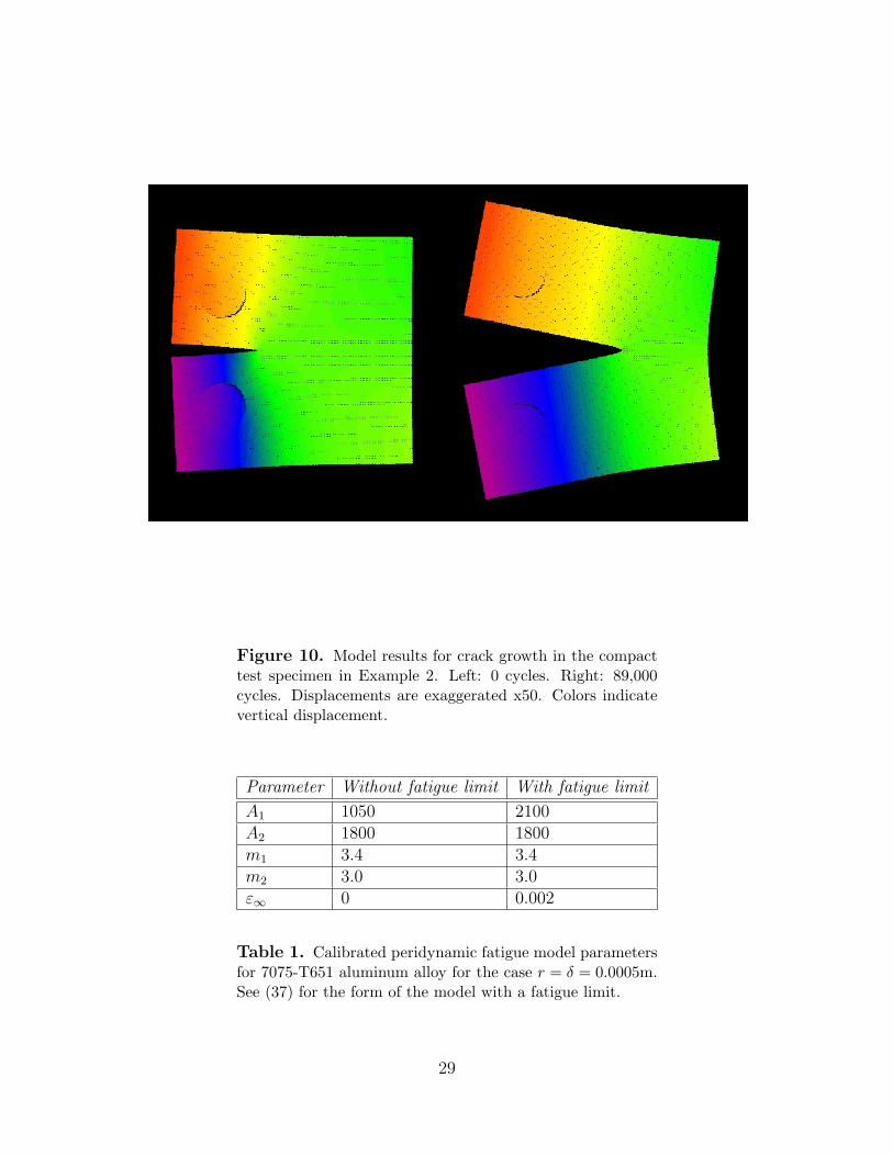
Figure 10. Model results for crack growth in the compacttest specimen in Example 2. Left: 0 cycles. Right: 89,000cycles. Displacements are exaggerated x50. Colors indicatevertical displacement.
Parameter Without fatigue limit With fatigue limit
A1 1050 2100A2 1800 1800m1 3.4 3.4m2 3.0 3.0ε∞ 0 0.002
Table 1. Calibrated peridynamic fatigue model parametersfor 7075-T651 aluminum alloy for the case r = δ = 0.0005m.See (37) for the form of the model with a fatigue limit.
29

Cra
ck g
row
th d
ista
nce (
mm
)
Load cycle (N x 1000) log10 ∆𝐾(𝑃𝑎 𝑚)
log10𝑑𝑎
𝑑𝑁 (𝑚)
Crack length Paris law plot
Experiment
Model
Model
Figure 11. Compact test specimen model results for R =0.1 (Example 3). Left: crack growth distance as a functionof loading cycle. Right: Paris law plot, including test data[36].
30

20
100
3
Figure 12. Geometry of the rod modeled in Example 3 (alldimensions are in mm).
grid spacing of approximately 0.5mm.
When the ends of the rod are rotated, a strain concentration occurs near the cavity. Thisleads to nucleation of fatigue damage at 1.2×10⁶ cycles. The damage progresses to growth offatigue cracks. These cracks grow approximately normal to the direction of maximum tensilestress, leading to a helical trajectory (Figure 13). Helical cracks are commonly observed inrods with a surface defect under torsion [1].
31

Initial cavity
Front view Rear view
Figure 13. Computed solution for the torsion exampleproblem after 3.5×10⁷ cycles. The two views are from oppo-site sides of the specimen. The white dot shows the locationof the initial cavity. Shading indicates magnitude of displace-ment.
32

6 Extensions
This section discusses some enhancements to the peridynamic fatigue model for special pur-poses.
6.1 Loading spectrum
In the development in Section 4, it is assumed that for any bond at any given time, there isa definite value of the cyclic bond strain ε(x, ξ) (although this value can change as damageevolves or boundary loading changes). However, in many applications, loading occurs oversome combination of frequencies. To derive a version of (11) that applies in this case, supposethat the bond strain consists of the superposition of J component angular frequencies ωj,each with amplitude εj:
ε =J∑j=1
1
2εj cos(ωjt).
This situation is described approximately by Miner’s rule [20, 14], which posits that failurewill occur when
J∑j=1
njNj
= 1 (34)
where nj is the number of cycles in component frequency ωj up to the time of failure tf , andNj is the number of cycles to failure if ωj were the only component frequency in the loadingspectrum. To apply Miner’s rule in the peridynamic model, use the definition of frequencyand (14) to obtain
nj =ωjtf2π
, Nj =1
Aεmj. (35)
Combine (34) and (35) and solve for tf :
tf =2π
A∑J
j=1 ωjεmj
.
Since, in the peridynamic model, λ changes from 1 to 0 over the time interval tf , we canmake the approximation dλ/dt = −1/tf . Therefore, the appropriate expression for changein remaining life of a given bond is found to be
λ(0) = 1,dλ
dt= − A
2π
J∑j=1
ωjεmj . (36)
In comparing this with the single-component expression (11), note that λ(t) is now treatedas a function of time rather than loading cycle N . In the above expressions, {A,m} wouldbe replaced by {A1,m1} and {A2,m2} in the nucleation and growth phases of fatigue, re-spectively.
33

6.2 Fatigue limit
In some materials, there is no fatigue damage if the loading is less than some lower limit onthe S-N curve. To incorporate such a fatigue limit into the peridynamic fatigue model, thenucleation phase in (11) is modified as follows:
λ(0) = 1,dλ
dN(N) =
{−A1(ε− ε∞)m1 , if ε > ε∞,0 otherwise.
(37)
where ε∞ is the lowest cyclic bond strain that results in damage over a very large number ofload cycles. An example of an S-N curve predicted by the peridynamic model with a fatiguelimit is shown in Figure 8.
6.3 Phase III
Ultimate failure of a structure due to the uncontrolled growth of a fatigue crack is sometimescalled “phase III.” Although this is the final culmination of the fatigue process in the failureof engineering components, it is controlled by the mechanics of static, rather than cyclicloading. To treat phase III within the present framework, we can include static fractureparameters as an additional bond failure criterion. Thus, a bond breaks irreversibly wheneither
λ(N) ≤ 0 or s+ ≥ s∗
where s∗ is the critical bond strain for failure under static loading, as described in Section 2.This critical strain can be calibrated to reproduce KIc in brittle materials [29].
6.4 Nonzero load ratio
For many materials, the load ratio R = P−/P+ has a strong effect on the rate of fatiguedamage, where P+ and P− are the loads applied at the two extremes of the cyclic loading.This effect motivates modification of the Paris law expression (24) to include dependenceon R, either explicitly or implicitly. Kujawski [8], and Dinda and Kujawski [5] consider aversion of the Paris law in which, in the present notation, the rate of crack growth is givenby
da
dN= c(K∗)M , K∗ = (K+)α
(K+ −max{0, K−}
)1−α(38)
where c, M , and α are constants, 0 ≤ α ≤ 1, and it is assumed that K+ ≥ 0.
To include the effect of load ratio in the peridynamic model, it is sufficient to observethat in an elastic model, the bond strains in the vicinity of a crack tip are proportional toK. Therefore, (11) can be modified in the same way as the Paris law to account for the loadratio. As an example, (38) can be adapted in the form
λ(0) = 1,dλ
dN(N) = −A2(ε
∗)m2 (39)
34

where, instead of the cyclic bond strain defined in (10), we have
ε∗ = (s+)α(s+ −max{0, s−}
)1−αand α has the same value as in (38). Even when this modified expression is used, (25)continues to apply.
35

7 Discussion
The peridynamic fatigue model described here retains the main advantages of the peridy-namic theory applied to crack growth: autonomous nucleation and growth of cracks in anydirection along complex paths in three dimensions. A key advantage of the model is thatthe actual loading cycles are not computed explicitly; only the + loading state is computed,with changing patterns of damage inside the body. With the help of the time-to-load cy-cle mappings discussed in Section 5, very large numbers of load cycles can be computed atreasonable computational cost.
It is possible that future work will reveal the detailed structure of the deformation fieldnear a crack tip in a peridynamic medium, thus providing the form of εcore and f explic-itly. This would allow β to be evaluated from (22), which would permit all four parame-ters A1, A2,m1,m2 to be evaluated directly from material test data without simulating theboundary value problem currently needed to find A2.
The examples in Section 5 used the LPS material model, but the fatigue model itself doesnot assume any particular material model. It seems possible to apply the fatigue model inconjunction with an elastic-plastic material model, with which it might be possible to studycrack closure effects. In this case, it would be necessary to avoid the assumption (33), whichimplicitly assumes linear elastic material response. Dropping this assumption would thenrequire both the + and − states to be computed everywhere in the body as a function oftime, rather than just the + state. This would involve simultaneously modeling the samebody twice, with the + and − boundary loads, with the identical damage state in bothbodies as time progresses. Fatigue cracks at interfaces between materials can be treatedby calibrating the parameters A and m separately for bonds that connect one material toanother.
36

References
[1] M. R. Bache and W. J. Evans. Tension and torsion fatigue testing of a near-alphatitanium alloy. International Journal of Fatigue, 14:331–337, 1992.
[2] S. Bordas and B. Moran. Enriched finite elements and level sets for damage toleranceassessment of complex structures. Engineering Fracture Mechanics, 73:1176–1201, 2006.
[3] O. K. Chopra. Mechanism and estimation of fatigue crack initiation in austenitic stain-less steels in LWR environments. Technical Report NUREG/CR-6787, ANL-01/25,Argonne National Laboratory, 2002.
[4] A. de Andres, J. L. Perez, and M. Ortiz. Elastoplastic finite element analysis of three-dimensional fatigue crack growth in aluminum shafts subjected to axial loading. Inter-national Journal of Solids and Structures, 36:2231–2258, 1999.
[5] S. Dinda and D. Kujawski. Correlation and prediction of fatigue crack growth fordifferent R-ratios using Kmax and ∆K+ parameters. Engineering Fracture Mechanics,71:1779–1790, 2004.
[6] W. Elbert. The significance of fatigue crack closure. In Damage Tolerance in AircraftStructures: A Symposium Presented at the Seventy-third Annual Meeting AmericanSociety for Testing and Materials, Toronto, Ontario, Canada, 21-26 June 1970, volume486, pages 230–242. ASTM International, 1971.
[7] R. Erdogan. Crack propagation theories. Technical Report CR-901, NASA, 1967.
[8] D. Kujawski. A fatigue crack driving force parameter with load ratio effects. Interna-tional Journal of Fatigue, 23:S239–S246, 2001.
[9] H. W. Liu and N. Iino. A mechanical model for fatigue crack propagation. In Proc. 2ndInternational Conference on Fracture, Paper 71, pages 812–823. Chapman-Hall, 1969.
[10] E. Madenci and E. Oterkus. Peridynamic Theory and Its Applications. Springer, NewYork, 2013.
[11] S. Majumdar and J. Morrow. Correlation between fatigue crack propagation and lowcycle fatigue properties, ASTM STP 559. In Fracture Toughness and Slow-Stable Crack-ing, Part 1, pages 159–182. ASTM International, 1974.
[12] R. C. McClung and H. Sehitoglu. On the finite element analysis of fatigue crack closure–1. Basic modeling issues. Engineering Fracture Mechanics, 33:237–252, 1989.
[13] R. C. McClung and H. Sehitoglu. On the finite element analysis of fatigue crack closure–2. Numerical results. Engineering Fracture Mechanics, 33:253–272, 1989.
[14] M. A. Miner. Cumulative damage in fatigue. Journal of Applied Mechanics, 12:159–164,1945.
37
[15] N. Moes, A. Gravouil, and T. Belytschko. Non-planar 3D crack growth by the ex-tended finite element and level sets–Part I: Mechanical model. International Journalfor Numerical Methods in Engineering, 53:2549–2568, 2002.
[16] N. Moes, A. Gravouil, and T. Belytschko. Non-planar 3D crack growth by the ex-tended finite element and level sets–Part II: Level set update. International Journal forNumerical Methods in Engineering, 53:2569–2586, 2002.
[17] MSC Software Corporation. MSC Fatigue. www.mscsoftware.com.
[18] O. Nguyen, E. A. Repetto, M. Ortiz, and R. A. Radovitzky. A cohesive model of fatiguecrack growth. International Journal of Fracture, 110:351–369, 2001.
[19] E. Oterkus, I. Guven, and E. Madenci. Fatigue failure model with peridynamic theory.In IEEE Intersociety Conference on Thermal and Thermomechanical Phenomena inElectronic Systems (ITherm), Las Vegas, NV, June 2010, pages 1–6, 2010.
[20] A. Palmgren. Die lebensdauer von kugellagern. Zeitschrift des Vereins Deutscher Inge-nieure, 68(14):339–341, 1924.
[21] P. Paris and F. Erdogan. A critical analysis of crack propagation laws. Journal of BasicEngineering, 85:528–533, 1963.
[22] N. Pugno, M. Ciavarella, P. Cornetti, and A. Carpinteri. A generalized Paris’ law forfatigue crack growth. Journal of the Mechanics and Physics of Solids, 54:1333–1349,2006.
[23] D. Radaj and M. Vormwald. Elastic-plastic fatigue crack growth. In D. Radajand M. Vormwald, editors, Advanced Methods of Fatigue Assessment, pages 391–481.Springer, New York, 2013.
[24] J. Shi, D. Chopp, J. Lua, N. Sukumar, and T. Belytschko. Abaqus implementation ofextended finite element method using a level set representation for three-dimensionalfatigue crack growth and life predictions. Engineering Fracture Mechanics, 77:2840–2863, 2010.
[25] J. Shi, J. Lua, H. Waisman, P. Liu, T. Belytschko, N. Sukumar, and Y. Liang.X-FEM toolkit for automated crack onset and growth prediction. In 49thAIAA/ASME/ASCE/AHS/ASC Structures, Structural Dynamics, and Materials Con-ference, Schaumburg, IL, April 2008, Paper AIAA 2008-1763, 2008.
[26] S. A. Silling. Reformulation of elasticity theory for discontinuities and long-range forces.Journal of the Mechanics and Physics of Solids, 48:175–209, 2000.
[27] S. A. Silling. Linearized theory of peridynamic states. Journal of Elasticity, 99:85–111,2010.
[28] S. A. Silling and E. Askari. A meshfree method based on the peridynamic model ofsolid mechanics. Computers and Structures, 83:1526–1535, 2005.
38

[29] S. A. Silling and E. Askari. A meshfree method based on the peridynamic model ofsolid mechanics. Computers and Structures, 83:1526–1535, 2005.
[30] S. A. Silling, M. Epton, O. Weckner, J. Xu, and E. Askari. Peridynamic states andconstitutive modeling. Journal of Elasticity, 88:151–184, 2007.
[31] S. A. Silling and R. B. Lehoucq. The peridynamic theory of solid mechanics. Advancesin Applied Mechanics, 44:73–168, 2010.
[32] Stewart A. Silling. EMU. http://www.sandia.gov/emu/emu.htm.
[33] D. C. Stouffer and J. F. Williams. A model for fatigue crack growth with a variablestress intensity factor. Engineering Fracture Mechanics, 11:525–536, 1979.
[34] N. Sukumar, D. L. Chopp, and B. Moran. Extended finite element method and fastmarching method for three-dimensional fatigue crack propagation. Engineering FractureMechanics, 70:29–48, 2003.
[35] T. Zhao and Y. Jiang. Fatigue of 7075-T651 aluminum alloy. International Journal ofFatigue, 30:834–849, 2008.
[36] T. Zhao, J. Zhang, and Y. Jiang. A study of fatigue crack growth of 7075-T651 aluminumalloy. International Journal of Fatigue, 30:1169–1180, 2008.
39

DISTRIBUTION:
1 MS 0899 Technical Library, 9536 (electronic copy)
1 MS 0115 OFA/NFE Agreements, 10112
40

v1.38