Permutations and Combinations 1 The Division Rule · 2019-09-12 · 4 Course Notes 9: Permutations and Combinations 2.1 The r-Combinations of a Set Generalizing the example that we

Massachusetts Institute of Technology Course Notes 96.042J/18.062J, Fall ’02: Mathematics for Computer ScienceProf. Albert Meyer and Dr. Radhika Nagpal

Permutations and Combinations

In Notes 8, we saw a variety of techniques for counting elements in a finite set: the Sum Rule, Inclusion-Exclusion, the Product Rule, tree diagrams, and permutations. We will now introduce yet another rule, the Division Rule, and one more concept, combinations. We will also learn techniques for counting elements of a finite set when limited repetition is allowed.

1 The Division Rule

The division rule is a common way to ignore “unimportant” differences when you are counting things. You can count distinct objects, and then use the division rule to “merge” the ones that are not significantly different.

We will state the Division Rule twice, once informally and then again with more precise notation.

Theorem 1.1 (Division Rule). If B is a finite set and f : A �→ B maps precisely k items of A to every item of B, then A has k times as many items as B.

For example, suppose A is a set of students, B is a set of tutorials, and f defines the assignment of students to tutorials. If 12 students are assigned to every tutorial, then the Division Rule says that there are 12 times as many students as tutorials.

The following two definitions permit a more precise statement of the Division Rule.

Definition 1.2. If f : A �→ B is a function, then f −1(b) = {a ∈ A | f (a) = b}.

That is, f −1(b) is the set of items in A that are mapped to the item b ∈ B. In the preceding example, f −1(b) is the set of students assigned to tutorial b.

This notation can be confusing, since f −1 normally denotes the inverse of the function f . With our definition, however, f −1(b) can be a set, not just a single value. For example, if f assigns no items in A to some element b ∈ B, then f −1(b) is the empty set. In the special case where f is a bijection, f −1(b) is always a single value, and so f −1 by our definition is just the ordinary inverse of f .

Definition 1.3. A function f : A �→ B is k-to-1 if for all b ∈ B, |f −1(b)| = k.

For example, if f assigns exactly 12 students to each recitation, then f is 12-to-1. Assuming k is non-zero, a k-to-1 function is always a surjection; every element of the range is mapped to by k > 0 elements of the domain.

We can now restate the Division Rule more precisely:

Theorem (Division Rule, restatement). If B is a finite set and f : A �→ B is k-to-1, then |A| = k|B|.Copyright © 2002, Prof. Albert R. Meyer.

� ��

2 Course Notes 9: Permutations and Combinations

Proof. Since B is finite, we can let n = |B| and let B = {b1, b2, . . . , bn}. Then we have:

A = f −1(b1) ∪ f −1(b2) ∪ · · · ∪ f −1(bn)

Equality holds because each side is contained in the other. The right side is contained in the left side because every set f −1(bi) is contained in A by the definition of f −1(bi). The left side is contained in the right, since every item in A maps to some bi, and therefore is contained in the set f −1(bi).

Furthermore, all of the sets f −1(bi) are disjoint. The proof is by contradiction. Assume for the purpose of contradiction that a ∈ f −1(bi) and a ∈ f −1(bj ) for some i �= j. The first inclusion implies f (a) = bi, but the second inclusion implies that f (a) = bj . This is a contradiction since f (a) denotes a unique item.

Since the sets f −1(bi) are disjoint, we can compute the cardinality of their union with the Sum Rule. Note that each set f −1(bi) has size k, since f is k-to-1.

|A| = |f −1(b1)| + |f −1(b2)| + · · · + |f −1(bn)| = k + k + · · · + k

n=|B| terms = k|B|

Example: Seating at a Round Table. In how many ways can King Arthur seat n knights at his round table? Two seatings are considered equivalent if one can be obtained from the other by rotation. For example, if Arthur has only four knights, then there are six possibilities as shown in Figure 1. Hereafter, we denote a seating arrangement in text by listing knights in square brackets in clockwise order, starting at an arbitrary point. For example, [1234] and [4123] are equivalent.

As a sign that we should bring in the division rule, the question points out that certain distinct seatings are equivalent, so should only be counted once—that is, we want to count equivalence classes instead of individual objects. The division rule is a good way to do this.

Claim 1.4. Arthur can seat n knights at his round table in (n − 1)! ways.

In particular, the claim says that for n = 4 knights there are (4 − 1)! = 3! = 6 orderings, which is consistent with the example in Figure 1.

Proof. The proof uses the Division Rule. Let A be the set of orderings of n knights in a line. Let B be the set of orderings of n knights in a ring. Define f : A �→ B by f ((x1, x2, . . . , xn)) = [x1x2 . . . xn].

The function f is n-to-1. In particular:

f −1([x1x2 . . . xn]) = { (x1, x2, x3, . . . , xn), (xn, x1, x2, . . . , xn−1) (xn−1, xn, x1, . . . , xn−2), . . .

(x2, x3, x4, . . . , x1)}

Course Notes 9: Permutations and Combinations 3

1 2

34

1 1

111

2

2

2 2

2

3 3

333 4

4

4

4

4

Figure 1: These are the 6 different ways that King Arthur can seat 4 knights at his round table. Two seatings differing only by rotation are considered equivalent. We denote a seating arrangement in text by listing knights in square brackets in clockwise order, starting at an arbitrary point. For example, the seatings in the top row can be denoted [1234], [2413], and [3421].

There are n tuples in the list of tuples, because x1 can appears in n different places in a tuple. By the Division Rule, |A| = n|B|. This gives:

|B| = |A| n

n! =

n = (n − 1)!

The second equality holds, because the number of orderings of n items in a line is n!, as we showed previously.

2 Combinations

We now use the Division Rule to find a formula for the number of combinations of elements from a set. One common pitfall in counting problems is mixing up combinations with permutations; try to keep track of which is which!

Example: Students and prizes. How many groups of 5 students can be chosen from a 180-student class to collaborate on a problem set?

Let A be the set of 5-permutations of the set of students. This number is P (180, 5) = 180 × 179 × 178 × 177 × 176. But that’s not really what we want—order of the 5 students in a group doesn’t matter. So let B be the set of 5-student groups. This is what we want. Let’s define a map f : A ⇒ B by ignoring the order. We claim that f is 5! to 1, in other words, 120 to 1. This is based on the number of ways that 5 students could be lined up. So, by the Division Rule,

|A| 180 × 179 × 178 × 177 × 176 |B| = 120

= 120

.

� �

� �

� ��


2.1 The r-Combinations of a Set

Generalizing the example that we just did, the Division Rule can be used to count the number of r-combinations of a set.

Definition 2.1. An r-combination of a set is a subset of size r.

For example, for the set {a, b, c}, we have the following three 2-combinations:

{a, b} {a, c} {b, c}

Understanding the distinction between r-combinations and r-permutations is important. The r-combinations of a set are different from r-permutations in that order does not matter. For example, the above set {a, b, c} has six 2-permutations:

(a, b) (a, c) (b, c) (b, a) (c, a) (c, b)

The collaboration groups of 5 students in previous example are the 5-combinations of the set of students in the class.

2.2 The number of r-Combinations (Binomial Coefficients)

The number of r-combinations of an n-element set comes up in many problems. The quantity is important enough to merit two notations. The first is C(n, r); this is analogous to the notation P (�n,�r) from before for the number of� r� permutations of an n-element set. The second notation is n

r , read “n choose r”. The values n r or C(n, r) are often called binomial coefficients because of

their prominent role in the Binomial Theorem, which we will cover shortly.

. This theorem is used all the time; remember it!The following theorem gives a closed form for n r

Theorem 2.2.

nr

=n!

(n − r)! r!

The theorem says, for example, that the number of 2-combinations of the three element set {a, b, c}is 3! = 3 as we saw above.(3−2)! 2!

180!Also, for example, the number of 5-combinations of the 180 element set of students is 175!5! .

Proof. The proof uses the Division Rule. Let X be a set with n elements. Let A be the set of r-permutations of X , and let B be the set of r-combinations of X . Our goal is to compute |B|. To this end, let f : A �→ B be the function mapping r-permutations to r-combinations that is defined by:

f ( (x1, x2, . . . , xr )

order matters(permutation)

) = {� x1, x2, . . . , xr }�

order does not matter (combination)

� �

� �

� �

� �

� �

� � � �

� � � �


The function f is r!-to-1. In particular:

f −1({x1, x2, . . . , xr }) = {(x1, x2, x3, x4, . . . , xr ), (x2, x1, x3, x4, . . . , xr ), . . . all r! permutations . . . }

By the Division Rule, |A| = r! |B|. Now we can compute the number of r-combinations of an n-element set, B, as follows:

|B| = |Ar!|

P (n, r)=

r! n!

= (n − r)! r!

2.3 Some interesting special cases

nBinomial coefficients are important enough that some special values of are worth remember-r ing:

n n! 0

= n! 0!

= 1 There is a single size 0 subset of an n-set.

n n!n

= 0! n!

= 1 There is a single size n subset of an n-set.

n n! = = n There are n size 1 subsets of an n-set.

1 (n − 1)! 1! n n!

n − 1 =

1! (n − 1)! = n There are n size (n − 1) subsets of an n-set.

Recall that 0! is defined to be 1, not zero.

Theorem 2.3. For all n ≥ 1, 0 ≤ r ≤ n,

n n = .

r n − r

Theorem 2.3 can be read as saying that the number of ways to choose r elements to form a subset of a set of size n is the same as the number of ways to choose the n − r elements to exclude from the subset. Put that way, it’s obvious. This is what is called a combinatorial proof of an identity: we write expressions that reflect different ways of counting or constructing the same set of objects and conclude that the expressions are equal. All sorts of complicated-looking and apparently obscure identities can be proved—and made clear—in this way.

Of course we can also prove Theorem 2.3 by simple algebraic manipulation:

n n! n! n! n = = = = .

r (n − r)! r! r! (n − r)! (n − (n − r))! (n − r)! n − r


3 Counting Poker Hands

In the poker game Five-Card Draw, each player is dealt a hand consisting of 5 cards from a deck of 52 cards. Each card in the deck has a suit (clubs ♣, hearts ♥, diamonds ♦, or spades ♠) and a value (A, 2, . . . , 10, J, Q,K). The order in which cards are dealt does not matter. We will count various types of hands in Five-Card Draw to show how to use the formula for r-combinations given in Theorem 2.2.

It may not be clear why we want to count the number of types of hands. The number of hands of a particular type tells us how “likely” we are to encounter such a hand in a “random” deal of the cards. Hands that are less likely are ranked higher than those that are more likely, and so will win over the more likely ones. Knowing the likelihood (or the number) of various hands can help us to figure out how to bet on the game.

3.1 All Five-Card Hands

How many different hands are possible in Five-Card Draw? A hand is just a 5-card subset of the 52-card deck. Therefore, the possible hands in Five-Card Draw are exactly the 5-combinations of

52!a 52-element set. By Theorem 2.2, there are �52

� = 47! 5! = 2, 598, 960 possible hands.5

Confusion between combinations and permutations is a common source of error in counting problems. For example, one might erroneously count the number of 5-card hands as follows. There are 52 choices for the first card, 51 choice for the second card given the first, . . . , and 48 choices for the fifth card given the first four. This totals 52 · 51 · 50 · 49 · 48 possible hands. The problem with this way of counting is that a hand is counted once for every ordering of the five cards; that is, each hand is counted 5! = 120 times. We accidentally counted r-permutations instead of r-combinations! To get the number of 5-combinations, we would have to divide by 120.

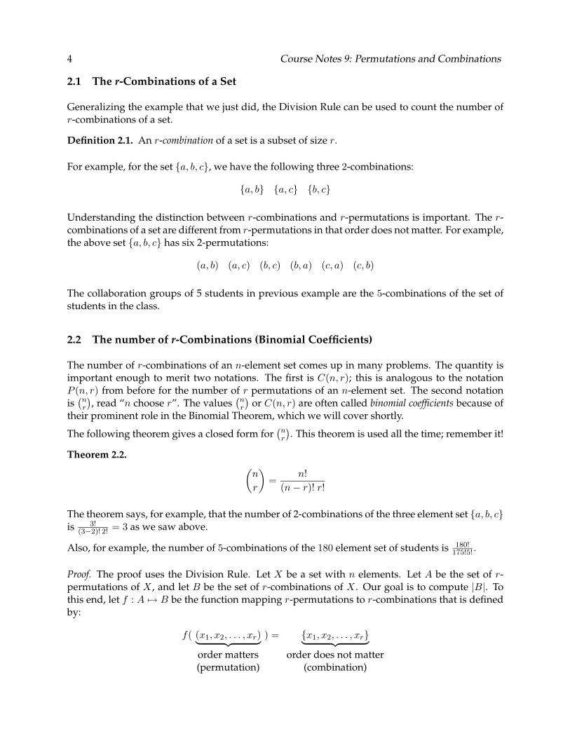
3.2 Hands with Four-of-a-Kind

How many hands are there with four-of-a-kind? For example, 9♠ 4♦ 9♣ 9♥ 9♦ has a four-of-a-kind, because there are four 9’s.

First we must choose one value to appear in all four suits from the set of 13 possible values (this follows the “tree diagram” approach to exploring distinct cases). There are 13 choices of this value, and if we pick one we can’t have any others (that would require 8 cards). So the choice of value gives 13 disjoint cases to count. After this choice, we have to choose one more card from the remaining set of 48. This can be done in

�48

� = 48 ways. In total, there are 13 · 48 = 624 hands1

with four-of-a-kind. The situation is illustrated by the tree diagram in Figure 2.

Here is a way to interpret the result that uses probability. If all �52

� hands are equally likely, then5

the probability that we are dealt a four-of-a-kind is

624 1 �52

� = 4165

. 5

In other words, we can only expect to get four-of-a-kind only once in every 4165 games of Five-Card Draw! (This is just a passing observation; we will talk about probability “for real” in a few weeks.)


A

2

3

2 spades2 clubs

K diamonds

K

chose fifth cardchose 4-tuplein 13 ways in 48 ways

Hands with 4-of-a-kind= 13 x 48 = 624

Figure 2: This (incomplete) tree diagram counts the number of hands with four-of-a-kind. There are 13 choices for the value appearing in all four suits. The fifth card in the hand can be any of the 48 cards remaining in the deck. This gives a total of 13 · 48 = 624 possible hands.

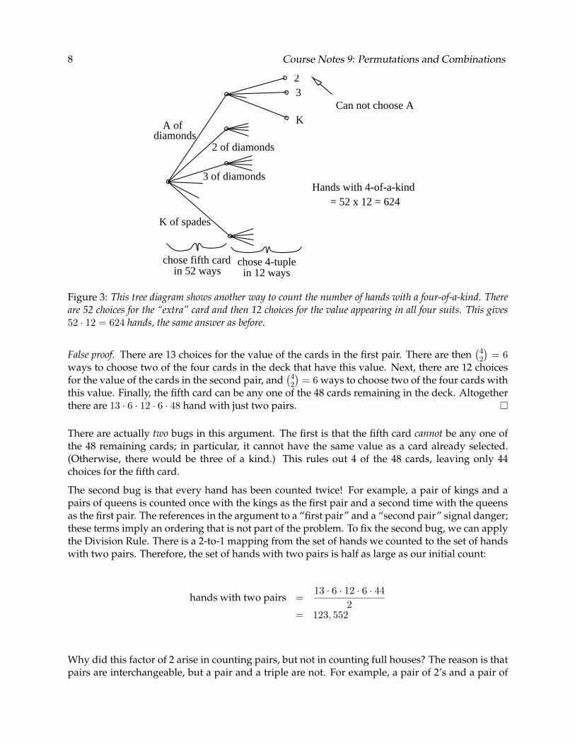
Mistakes are easy to make in counting problems. It is a good idea to check a result by counting the same thing in another way. For example, we could also count the number of hands with a four-of-a-kind as follows. First, there are 52 ways to choose the “extra” card. Given this, there are 12 ways to choose the value that appears in all four suits. (We cannot choose the value of the first card.) The possibilities are illustrated by the tree diagram in Figure 3. By this method, we find that there are 52 · 12 = 624 four-of-a-kind hands. This is consistent with our first answer (which is a good thing).

3.3 Hands with a Full House

A full house is a hand with both a three-of-a-kind and a two-of-a-kind. For example, the hand 7♠ 7♦ J ♣ J ♥ J ♦ is a full house because there are three jacks and two sevens. How many full house hands are there?

Then we can pick any three ofWe can choose the value that appears three times in 13 ways.�4�

the four cards in the deck with this value; this can be done in 3 = 4 ways. There are then 12 remaining choices for the value that appears two times. We can pick any two of the four cards�

4�

with this value; this can be done in 2 = 6 ways.

The total number of full house hands is therefore 13 · 4 · 12 · 6 = 3744. This is 6 times greater than the number of hands with a four-of-a-kind. Since a four-of-a-kind is rarer, it is worth more in poker!

3.4 Hands with Two Pairs

How many hands are there with two pairs, but no three- or four-of-a-kind?


Hands with 4-of-a-kind

diamondsA of

2 of diamonds

3 of diamonds

K of spades

chose fifth cardin 52 ways

chose 4-tuplein 12 ways

= 52 x 12 = 624

23

KCan not choose A

Figure 3: This tree diagram shows another way to count the number of hands with a four-of-a-kind. There are 52 choices for the “extra” card and then 12 choices for the value appearing in all four suits. This gives 52 · 12 = 624 hands, the same answer as before.

�4�

False proof. There are 13 choices for the value of the cards in the first pair. There are then 2 = 6 ways to choose two of the four cards in the deck that have this value. Next, there are 12 choices�

4�

for the value of the cards in the second pair, and 2 = 6 ways to choose two of the four cards with this value. Finally, the fifth card can be any one of the 48 cards remaining in the deck. Altogether there are 13 · 6 · 12 · 6 · 48 hand with just two pairs.

There are actually two bugs in this argument. The first is that the fifth card cannot be any one of the 48 remaining cards; in particular, it cannot have the same value as a card already selected. (Otherwise, there would be three of a kind.) This rules out 4 of the 48 cards, leaving only 44 choices for the fifth card.

The second bug is that every hand has been counted twice! For example, a pair of kings and a pairs of queens is counted once with the kings as the first pair and a second time with the queens as the first pair. The references in the argument to a “first pair” and a “second pair” signal danger; these terms imply an ordering that is not part of the problem. To fix the second bug, we can apply the Division Rule. There is a 2-to-1 mapping from the set of hands we counted to the set of hands with two pairs. Therefore, the set of hands with two pairs is half as large as our initial count:

13 · 6 · 12 · 6 · 44hands with two pairs =

2 = 123, 552

Why did this factor of 2 arise in counting pairs, but not in counting full houses? The reason is that pairs are interchangeable, but a pair and a triple are not. For example, a pair of 2’s and a pair of

�


9’s is the same as a pair of 9’s and a pair of 2’s. On the other hand, a pair of 2’s and a triple of 9’s is different from a pair of 9’s and a triple of 2’s!

To check our result, we can count the number of hands with two pairs in a completely different way. The number of ways to choose the values for the two pairs is

�13

� . We can choose suits for2

each pair in �4�

= 6 ways, and we can choose the remaining card in 44 ways as before. This gives:2 �13 2

· 6 · 6 · 44 = 123, 552

This is the same answer as before. Two pairs turn out to be 33 times more likely than a full house; as one would expect, a full house beats two pairs in poker!

The following optional sections contain similar examples of poker hand counting.

3.5 Three of a kind, two different

[Optional]

There are �13�

ways to choose the rank for the three-of-a-kind, and once that is chosen, there are �4�

ways to choose the1 3

three cards. Once we have the three-of-a-kind, there are �12�

ways to choose the two ranks for the other two cards. And�4� 2

then for each of these ranks, there are 1 ways to choose the single card of that rank. The total is: � ��

13 4 12 4 4 = 54, 912.

1 3 2 1 1

Since this is fewer than the hands with two pairs, this is ranked higher.

3.6 One pair, others all different

[Optional] �4�

There are �13�

ways to choose the rank for the pair, and then 2 ways to choose the two cards of that rank. Then there

1

are �12�

ways to choose the ranks of the remaining three cards, and for each of these ranks, �4�

ways to choose the single3 1

card of that rank. The total is: � �� 13 4 12 4 4 4

= 1, 098, 240 1 2 3 1 1 1

3.7 Four different ranks

[Optional]

We have analyzed all the actual poker hands based on the numbers of cards of different ranks (4-1, 3-2, 3-1-1, 2-2-1, 2-1-1-1).

How many hands have all 5 cards of different ranks? That’s the total number of hands minus the sum of the numbers of hands of these five kinds, or

2, 598, 960 − 1, 098, 240 − 123, 552 − 54, 912 − 3, 744 − 624 = 1, 317, 888.

What is wrong with the following counting argument?

False counting argument. There are 52 choices for the first card, 48 choices for the second card given the first, 44 choices for the third given the first two, etc. After each card, the number of remaining choices drops by four, since we cannot

� �


subsequently pick the card just taken or any of the other three cards with the same value. This gives 52 · 48 · 44 · 40 · 36 hands with no pair. Is this answer right?

The references to “first card”, “second card”, . . . are a warning signal that we may be inadvertently counting an ordered set. To be sure, we can check how many times a particular hand is counted. Consider the hand A♥ K♠ Q♣ J ♣ 10♥. We could have obtained this hand by drawing cards in the order listed, but we could also have drawn them in another order. In fact, we counted this hand once for every possible ordering of the five cards, and in fact, every hand is counted 5! = 120 times! We can correct our initial answer by applying the Division Rule. This gives:

52 · 48 · 44 · 40 · 36hands with no pairs =

120 = 1, 317, 888

And still another way: There is another way to count the hands with no pairs that avoids this confusion. Since there are no pairs, no two cards have the same value. This means that we could first choose 5 distinct values from the set of 13 possibilities. Then we could choose one of the four suits for each of the five cards. This gives:

13hands with no pairs = · 45

5

13 · 12 · 11 · 10 · 9 = · 45

5 · 4 · 3 · 2 · 1 = 1, 317, 888

This is the same answer as before. Notice that the number of hands with no pairs is more than half of all the hands. This means that in more than half our games of Five-Card Draw, we will not have even one pair!

3.8 Hands with Every Suit

[Optional]

How many hands contain one card of every suit? Such a hand must contain two cards from one suit and one card from each of the other three suits. Again, we can count in two ways.

First count. Pick one card from each suit. This can be done in 134 ways. Then pick any one of the remaining 48 cards. This gives a total of 134 · 48 hands. However, we have overcounted by two, since the two cards with the same suit could be picked in either order. Accounting for this, there are 13

4

2 ·48 = 685, 464 hands.

Second count First, we can pick the suit that contains two cards in four ways. Then we can pick values for these two cards in

�13 2 � �� 3

hands with all suits = 13 13

4 2 1

13 · 12 = 4 · · 13 · 13 · 13

2 = 685, 464

� ways. Finally, we can pick a card from each of the other three suits in 13 ways. This gives:

More than a quarter of all Five-Card Draw hands contain all suits.

3.9 Reminders

To make sure that you get the right answer when counting:

1. Look at a sample 5-card hand (or a sample of whatever you are counting) and make sure that it is covered once and only once in your count.


2. Try counting by two different ways and check that you get the same answer.

For example, when we first counted the number of hands with no pairs, we discovered that we had massively overcounted; a sample hand was actually covered 120 times by our count! We corrected this answer by applying the Division Rule, and we counted the same thing again in a different way as a double-check.

4 The Magic Trick

There is a Magician and an Assistant. The Assistant goes into the audience with a deck of 52 cards while the Magician looks away. Five audience members are asked to select one card each from the deck. The Assistant then gathers up the five cards and announces four of them to the Magician. The Magician thinks for a time and then correctly names the secret, fifth card! Only elementary combinatorics underlies this trick, but it’s not obvious how. (The reader should take a moment to think about this; the Assistant doesn’t cheat.)

4.1 How the Trick Works

The Assistant has somehow communicated the secret card to the Magician just by naming the other four cards. In particular, the Assistant has two ways to communicate. First, he can announce the four cards in any order. The number of orderings of four cards is 4! = 24, so this alone is insufficient to identify which of the remaining 48 cards is the secret one. Second, the Assistant can choose which four of the five cards to reveal. The amount of information that can be conveyed�

5�

this way is harder to pin down. The Assistant has 4 = 5 ways to choose the four cards revealed, but the Magician can not determine which of these five possibilities the Assistant selected, since he does not know the secret card! Nevertheless, these two forms of communication allow the Assistant to covertly reveal the secret card to the Magician.

Here is an overview of how the trick works. The secret card has the same suit as the first card announced. Furthermore, the value of the secret card is offset from the value of the first card announced by between 1 and 6. See Figure 4. This offset is communicated by the order of the last three cards.

Here are the details. The audience selects five cards and there are only 4 suits in the deck. There-fore, by the Pigeonhole Principle, the Assistant can always pick out two cards with the same suit. One of these will become the secret card, and the other will be the first card that he announces.

Here is how he decides which is which. Note that for any two card numbers, one is at most six clockwise steps away from the other in Figure 4. For example, if the card numbers are 2 and Q, then 2 is three clockwise steps away from Q. The Assistant ensures that the value of the secret card is offset between 1 and 6 clockwise steps from the first card he announces.

The offset is communicated by the order that the Assistant announces the last three cards. The Magician and Assistant agree in advance on an order for all 52 cards. For example, they might use:

A ♣, 2 ♣, . . . ,K ♣, A ♦, . . . ,K ♦, A ♥, . . . ,K ♥, A ♠, . . . ,K ♠,


K A

2

3

4

5

67

8

9

10

J

Q

by ordering of

this card first.Assistant reveals

This is thesecret card.

last 3 cards.

Offset passed

Figure 4: The 13 possible card values can be ordered in a cycle. For any two distinct values, one is offset between 1 and 6 clockwise steps from the other. In this diagram, 3 is offset five steps from J . In the card trick, the value of the secret card is offset between 1 and 6 steps from the first card announced. This offset is communicated by the order of the last three cards named by the Assistant.

though any other order will do as well—so long as the Magician and his Assistant use the same one :-). With this order, one of the last three cards announced is the smallest (S), one is largest (L), and the other is medium (M ). The offset is encoded by the order of these three:

SML = 1 SLM = 2 MSL = 3 MLS = 4 LSM = 5 LMS = 6

For example, suppose that the audience selects 3♥ 8♦ A♠ J ♥ 6♦. The Assistant picks out two cards with the same suit, say 3♥ and J ♥. The 3♥ is five clockwise steps from J ♥ in Figure 4. So the Assistant makes 3♥ the secret card, announces J ♥ first, and then encodes the number 5 by the order in which he announces the last three cards: A♠ 6♦ 8♦ = LSM = 5.

4.2 Same Trick with 4 Cards?

Could the same magic trick work with just 4 cards? That is, if the audience picks four cards, and the Assistant reveals three, then can the Magician determine the fourth card? The answer turns out to be “no”. The proof relies on the Pigeonhole Principle.

Theorem 4.1. The magic trick is not possible with 4 cards.

Proof. The audience can select any 4-combination of cards; let A be the set of all such 4-combinations. The Assistant can announce any 3-permutation of cards; let B be the set of all such 3-permutations. The formulas for r-combinations and r-permutations give the following sizes for A and B:


|A| = C(n, r) 52!

= 48! 4!

= 270, 725

|B| = P (n, r) 52!

= 49!

= 132, 600

The Assistant sees a 4-combination of cards selected by the audience and must announce a 3-permutation to the Magician. Let f : A �→ B be the function that the Assistant uses in mapping one to the other. Since |A| > |B|, the Pigeonhole Principle implies that f maps at least two 4-combinations to the same 3-permutation. That is, there are two different sets of four cards that the audience can pick for which the Assistant says exactly the same thing to the Magician.

For these two sets of four cards, three cards must be the same (since the Assistant announces the same three cards in both cases) and one card must be different (since the two sets are different). For example, these might be the two sets of four cards for which the Assistant says exactly the same thing to the Magician:

3♥ 8♦ A♠ J ♥

3♥ 8♦ A♠ K♦

In this case, the Assistant announces 3♥ 8♦ A♠ in some order. The magician is now stuck; he can not determine whether the remaining card is J ♥ or K♦.

There are many variants of the magic trick. For example, if the audience picks 8 cards, then revealing 6 to the Magician is enough to let him determine the other two. This sort of subtle transmission of information is important in the security business where one wants to prevent information from leaking out in undetected ways. This is actually a whole field of study.

4.3 Hall’s Theorem applied to the Magic Trick

We know how the “Magic” trick works in which an Assistant reads four cards from a five card hand and the Magician predicts the fifth card. We also know the trick cannot be made to work if the Assistant only shows three cards from a four card hand, because there are fewer sequences of three out of 52 cards than there are 4-card hands out of 52 cards.

So the question is, when can the trick be made to work? For example, what is the largest size deck for which our trick of reading 4 cards from a 5-card hand remains possible?

An elegant result known as Hall’s Marriage Theorem allows us to answer the general question of when the trick can be made to work. Namely, the trick is possible using h-card hands chosen from an n-card deck, with the Assistant reading r of the h cards iff

P (h, r) ≥ C(n − r, h − r). (1)


In particular, using h = 5-card hands and revealing 4 = r cards, we can do the trick with an n-card deck as long as 120 = P (5, 4) ≤ C(n − 4, 1) = n − 4. So we can do the trick with a deck of up to size 124.

For example, we could still do the trick, with room to spare, if we combined a red deck with a blue deck to obtain a 104-card deck. Of course it’s not clear whether with the double-size deck there will be a simple rule for determining the hidden card as there is with the 52-card deck, but Hall’s Theorem guarantees there will be some rule.

4.4 Hall’s Marriage Theorem

The Magician gets to see a sequence of 4 cards and has to determine the 5th card. He can do this if and only if there is a way to map every 5-card hand into a sequence of 4 cards from that hand so that no two hands map to the same sequence. That is, there needs to be an injection from the set of 5-card hands into the 4-card sequences, subject to the constraint that each 5-card hand maps to a 4-card sequence of cards from that hand.

This is an example of a Marriage Problem. The traditional way to describe such a problem involves having a set of women and another set of men. Each women has a list of men she is willing to marry and who are also willing to marry her. The Marriage Problem is to find, for each woman, a husband she is willing to marry. Bigamy is not allowed: each husband can have only one wife. When such a matching of wives to husbands is possible, that particular Marriage Problem is solvable.

For our card trick, each 5-card hand is a “woman” and each 4-card sequence as a “man.” A man (4-card sequence) and woman (5-card hand) are willing to marry iff the cards in the sequence all occur in the hand.

Hall’s Theorem gives a simple necessary and sufficient condition for a Marriage Problem to be solvable.

Theorem 4.2 (Hall’s Marriage Theorem1). Suppose a group of women each have a list of the men they would be willing to marry. Say that a subset of these women has enough willing men if the total number of distinct men on their lists is at least as large as the number of women in the subset. Then there is a way to select distinct husbands for each of the women so that every husband is acceptable to his wife iff every subset of the women has enough willing men.

Hall’s Theorem can also be stated more formally in terms of bipartite graphs.

Definition. A bipartite graph, G = (V1, V2, E), is a simple graph whose vertices are the disjoint union of V1 and V2 and whose edges go between V1 and V2, viz.,

E ⊆ {{v1, v2} | v1 ∈ V1 and v2 ∈ V2} .

A perfect matching in G is an injection f : V1 → V2 such that {v, f (v)} ∈ E for all v ∈ V1.

For any set, A, of vertices, define the neighbor set,

N (A) ::= {v | ∃a ∈ A {a, v} ∈ E} .

A set A ⊆ V1 is called a bottleneck if |A| > |N (A)|.


Theorem (Hall). A bipartite graph has a perfect matching iff it has no bottlenecks.

A simple condition ensuring that a bipartite graph has no bottleneck is given in the in-class problems for Wednesday, Oct. 30, 2002. This condition is easy to verify for the graph describing the card trick, and it implies that inequality (1) is necessary and sufficient for the trick to be possible.

4.4.1 Other Examples [Optional]

[Optional]

Hall’s Marriage Theorem guarantees the possibility of selecting four cards of distinct suits, one each from any four separate piles of 13 cards from a standard deck of 52.

Likewise, there will always be 13 cards of distinct denominations, one from each of 13 piles of four cards. In this case, think of each pile as the set of one to four the distinct card denominations that appear in that pile. Notice that among any k piles of cards at least k distinct denominations appear—by the Generalized Pigeonholing Principle, there are at least that many distinct denominations among any 4k cards. Thus the existence of one card of each denomination spread out across 13 piles is assured by the Theorem.

Pulling in this big theorem is comforting—but not completely satisfactory. Although it assures us that these feats can always be accomplished, it gives absolutely no indication of how to perform them! Trial and error works well enough for the simple four-pile problem, but not with 13 piles. Is there a general procedure for pulling out a selection of distinct denominations from 13 piles of four cards?

Fortunately there is: choose an arbitrary pile containing an Ace, then one containing a two, and so on, doing this for as long as possible until you get stuck. Place these selected piles in a row. Suppose you have selected a total of ten piles, containing an Ace, and two through ten, respectively. This scenario leaves three untouched piles. If any of the 12 cards in those three piles is a Jack, Queen, or King then you are not really stuck; you can continue a little further (but perhaps not in the usual sequential order). If you are truly stuck, select any card in, say, the 11th pile, and go to one of the ten piles that corresponds to the number of that card. Thus if you select a three you go to the third pile. Turn a card in that third pile over (to make it conspicuous) and move to the pile that corresponds to the number of that turned card. Keep doing this to create a chain of piles and turned cards, until you eventually hit upon a pile that contains a card not in the initial list; in our case, until we come upon a Jack, Queen, or King. (Note: One can prove that you will not fall into a closed loop of choices.) Now shift all the piles one place back along the chain of piles to obtain a configuration that allows you to add one more pile to the initial list of ten. Repeat this process until you solve the puzzle completely.

4.4.2 Proof of Hall’s Theorem by Induction [Optional]

[Optional]

This method of chain shifting is known in the literature as the technique of augmenting paths and is the basis for efficient ways to find perfect matchings and to solve related “network flow” problems. This is described in many combinatorics texts2, but we shall not develop this method here.

Instead, we’ll go back to the man-woman marriage terminology and give a simple proof by:

Proof. Strong induction on the number, n, of women.

Base case (n = 1). If there is just a single woman with at least one name on her list, then she can simply marry the first man on her list.

Induction step (n > 1).

Case I. Suppose these women’s lists satisfy the stronger condition that among any r lists, 1 ≤ r < n, at least r + 1 distinct names are mentioned. Select one woman. She has at least two names on her list (r = 1 case). Have her marry one of these men (call him “Poindexter”). This leaves n − 1 women to marry.

2For example, Ian Anderson presents a procedural proof using augmenting paths in his book A First Course in Combinatorial Mathematics, Oxford Applied Mathematics and Computer Science Series, Clarendon Press, Oxford, 1974.

� � � � �


The lists possessed by these n − 1 women have the property that among any r of them (1 ≤ r < n) at least r + 1 distinct names are mentioned. One of these names could be Poindexter’s who is no longer available for marriage. But we can still say that among any r lists, at least r distinct names of available men are mentioned. This is all we need to invoke the induction hypothesis for these remaining n − 1 women. Thus we have a means to marry all n women in this scenario.

Case II. Suppose this stronger condition does not hold. Thus there is subgroup of r0 women (1 ≤ r0 < n) such that among their lists precisely r0 distinct names are mentioned. By the strong induction hypothesis for r0 < n, we can marry these women. This leaves m = n − r0 < n women to consider.

Is it true that among these m women’s lists any r of them (1 ≤ r ≤ m) mention at least r distinct names of available men? The answer is yes! If not, say some r of these women mention fewer than r available men. Then these r women plus the r0 women above have mentioned fewer in r0 + r men in total. This contradicts the property satisfied by these lists.

Thus we can invoke the strong induction hypothesis for the remaining m women and successfully have them marry as well. This completes the proof by induction.

Problem 1. The induction proof can read as a recursive procedure to construct a marriages for n woman in terms of constructing marriages for smaller sets of women. Why isn’t this procedure very efficient?

Problem 2. A deck of cards is shuffled and dealt into 26 piles of two cards. Is it possible to select a black Ace from one pile, a Red ace from another, a black two from a third, a red two from a fourth, and so on all the way down to a black King and a red King from the two remaining piles?

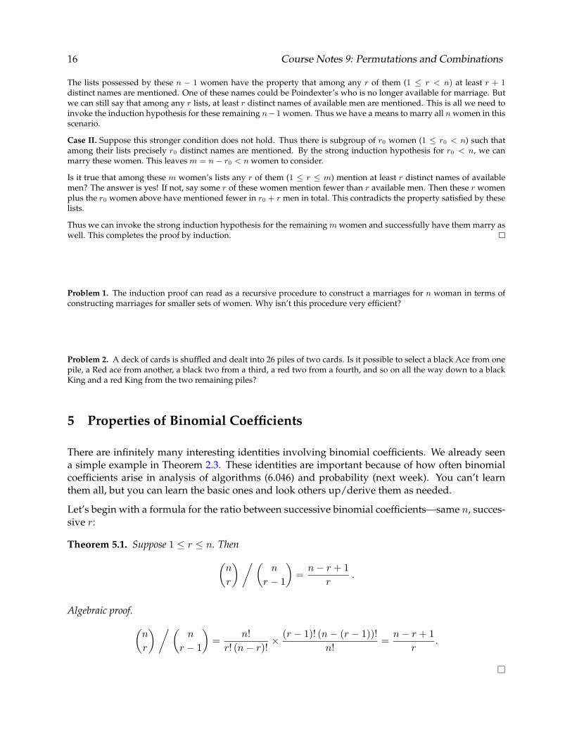
5 Properties of Binomial Coefficients

There are infinitely many interesting identities involving binomial coefficients. We already seen a simple example in Theorem 2.3. These identities are important because of how often binomial coefficients arise in analysis of algorithms (6.046) and probability (next week). You can’t learn them all, but you can learn the basic ones and look others up/derive them as needed.

Let’s begin with a formula for the ratio between successive binomial coefficients—same n, successive r:

Theorem 5.1. Suppose 1 ≤ r ≤ n. Then � � � � � n n n − r + 1

= . r r − 1 r

Algebraic proof.

n r

nr − 1

=n!

r! (n − r)! ×

(r − 1)! (n − (r − 1))! n!

=n − r + 1

r.

�

� �

� � � �

� �

� � � �

� �

� �


Combinatorial proof. Consider choosing a committee of size r and a leader, from n �people. One nway is to first pick the r − 1 commons and then their leader; this can be done in r−1 (n − (r − 1))

ways. Another way is to pick the r committee members first and then pick a leader from among nthem; this can be done in r ways. Thus,r

n n r − 1

(n − r + 1) = r. r

This ratio is greater than 1 if r < n+1 and less than 1 if r > n+1 . This says that the successive2 2 coefficients increase until r reaches n+1 and then decrease, i.e., they are unimodal like the curve in2 Figure 5.

Figure 5: Bell Curve

In fact, the binomial coefficients form a real bell curve. These arise on examinations in a natural way. Suppose that a test has n questions. Then the bell curve describes, for every r, the number

nof ways the student can get exactly r of the questions right, namely . If we suppose that each r student taking the test is doing random guessing, so is equally likely to get each of the n questions right or wrong, then these coefficients turn out to be proportional to the number of students that get those numbers of questions right. (We’ll see this when we do probability.)

Another identity:

Theorem 5.2. Suppose 1 ≤ r ≤ n. Then

n n n − 1 = .

r r r − 1

Algebraic proof.

n n! n (n − 1)!= =

r r!(n − r)! r (r − 1)!(n − r)! n (n − 1)! n n − 1

= = . r (r − 1)! ((n − 1) − (r − 1))! r r − 1

� �

� � � �

� � � �

� �

� �


Combinatorial proof. Consider choosing a committee of size r and a leader, fr� om� n people. One n−1way is to first pick the leader and then his r − 1 subjects; this can be done in n r−1 ways. Another

way is to pick the r committee members first and then pick a leader from among them; this can be ndone in r ways. Thus,r

n − 1 n n = r.

r − 1 r

Now an important theorem due to Pascal:

Theorem 5.3 (Pascal). Suppose 1 ≤ r ≤ n − 1. Then � � � � � � n n − 1 n − 1

= + . r r r − 1

This is probably our most important identity, since it gives a kind of recurrence for binomial coefficients. Memorize it!

Algebraic proof.

n − 1 n − 1 + =

r r − 1

=

=

=

=

(n − 1)! (n − 1)! r!(n − 1 − r)!

+ (r − 1)!(n − r)!

(n − r)(n − 1)! (n − 1)!

r!(n − r)! + r

r!(n − r)! (n − 1)!

n r!(n − r)!

n! r!(n − r)! n r

Combinatorial proof. We use case analysis (a tree diagram) and the sum rule. Let S ::= {1, . . . , n}. Let A be the set of r-element subsets of S. Let B be the set of r-element subsets of S that contain n. Let C be the set of r-element subsets of S that don’t contain n.

Then A = B ∪ C, and B and C are disjoint. So |A| = |B| + |C|, by the Sum Rule. But now we can get expressions for |A|, |B| and |C| as numbers of combinations:

•

n |A| = . r

� �

� �

�


•

n − 1 |B| = r − 1

.

This is because, in addition to n, another r − 1 elements must be chosen from {1, . . . , n − 1}.

•

n − 1 |C| = . r

This is because r elements must be chosen from {1, . . . , n − 1}.

So (by the Sum Rule) � � � � � � n n − 1 n − 1

= |A| = |B| + |C| = r − 1

+ . r r

Pascal’s theorem has a nice pictorial representation: The row represents n, starting with 0 in the top row. Successive elements in the row represent r, starting with 0 at the left.

1

1

1

1

1

1

1

2

3 3

4 6 41 1

Figure 6: Pascal’s triangle.

(Notice that it’s just the double-induction matrix “reshaped”.)

This triangle has lots of nice properties. Experiment with it. For example, what happens if we add the coefficients in one row?

For the following two theorems we provide their combinatorial proofs, only. The corresponding algebraic proofs are easy inductive arguments.

Theorem 5.4. Suppose n is any natural number. Then

n � � n

= 2n . r

r=0

� �

� � � �

�

�


Combinatorial proof. Again, we use case analysis and the sum rule for disjoint unions. There are 2n

different subsets of a set of n elements. Decompose this collection based on the sizes of the subsets. That is, let Ar be the collection of subsets of size r. Then the set of all subsets is the disjoint union

n∪r Ar . There are subsets of size r, for r = 0, 1, . . . , n. Hence the theorem follows. r

[Optional]

Theorem 5.5 (Vandermonde). Suppose 0 ≤ r ≤ m, n. Then � � � �� m + n � m n

= r r − k k

k=0

r

Combinatorial proof. Again, we use case analysis with the sum and product rules. Suppose there are m red balls and m+n n blue balls, all distinct. There are ways to choose r balls from the two sets combined. That’s the LHS. Now

r decompose this collection of choices based�on� how many of the chosen balls are blue. For any k, 0 ≤ k ≤ r, �there��are�

m n m n r−k ways to choose r − k red balls, and

k ways to choose k blue balls. By the product rule, that makes r−k k

ways to choose r balls such that k of them are blue. Adding up these numbers for all k gives the RHS.

5.1 The Binomial Theorem

An important theorem gives the coefficients in the expansion of powers of binomial expressions. It turns out they are binomial coefficients—thus the name!

Theorem 5.6. Suppose n ∈ N. Then

n � � n

(x + y)n = x k y n−k . k

k=0

Example 5.7. (x + y)4 = 1x4 + 4x3y + 6x2y2 + 4xy3 + 1y4 .

Algebraic proof. By induction, using Pascal’s identity.

Combinatorial proof. Consider the product

(x + y)n = (x + y)(x + y)(x + y)(x + y) · · ·

This product has n factors. To expand this product, we generate individual terms of the sums by selecting (in all possible ways) one of the two variables inside each factor to get an n-variable product. If we select k “x” variables and n − k “y” variables, we get a term of the form xk yn−k . Then we gather all those terms together. So how many ways do we get such�a �term? Each xk yn−k

nterm selects x from k of the factors and y from the other n − k. So there are k ways of choosing which factors have x.

The binomial theorem can be used to give slick proofs of some binomial identities, for example:

Theorem 5.8. n � �

n = 2n .

k k=0

�

� � � �


Proof. Plug x = 1, y = 1 into binomial theorem.

Theorem 5.9.

n � � n

(−1)k = 0. k

k=0

Proof. Plug x = −1, y = 1 into binomial theorem.

The combinatorial interpretation is as follows: the number of ways of selecting an even number of elements from a set of n equals the number of ways of selecting an odd number. This works for both even and odd n.

Example 5.10. Consider n = 5. We can choose an odd-size set �5� �

5� �

5�

+ + = 5 + 10 + 1 = 161 3 5

ways. We can choose an even-size set �5� �

5� �

5�

+ + = 1 + 10 + 5 = 160 2 4

ways.

Example 5.11. n = 6: There are 6 + 20 + 6 = 32 odd sets. There are 1 + 15 + 15 + 1 = 32 even sets.

For odd n, this is intuitive (choosing an even set leaves an odd set). For even n, it may be somewhat surprising—there is no obvious bijection between the even and odd sets. Theorem 5.9 can also be proven using inclusion/exclusion in a tricky way.

6 Principle of Inclusion and Exclusion

Now we return to the Principle of Inclusion-Exclusion from last week. Our binomial coefficient identities give us a way to prove this theorem, via our alternating sum identity (proved by binomial theorem). Recall the Inclusion-Exclusion theorem: � � � � Theorem 6.1. | i Ai| = |Ai| −

i<j |Ai ∩ Aj | +

i<j<k |Ai ∩ Aj ∩ Ak | − · · ·

i

The theorem can be proved by induction on the number of sets, but this approach is messy . Instead we will give a combinatorial proof using binomial coefficients. � Proof. Each term in the summation counts certain elements in i Ai. We prove that every element of this union is counted exactly once. So, consider any particular element a, and suppose it is in exactly r of the sets Ai. We see how many times a is counted by each term.

rIn the first term, a is counted r = 1 times, once for each of the sets that contains it. In the second rterm, a is counted 2 times, once for each of the pairs of sets that contain it. In the third term, a is

� � � �

�

� �

� ��


r rcounted 3 times, . . . , and in the rth term, a is counted r = 1 times. The terms alternate signs, so the total number of times a is counted is: � � � � � � � �

r r r r 1

− 2

+3

− · · · − (−1)r . r

But Theorem 5.9 implies that

r � � n

(−1)k = 0. k

k=0

rThis implies that the sum above is equal to 0 = 1. That is, a is counted exactly once, as needed.

7 r-Permutations with Repetition

We now turn to permutations and combinations where elements are allowed to repeat. An r- permutation with repetition of a set S is the number of ways to choose r elements from S with repetition allowed and where order matters. For example, there are nine 2-permutations with repetition of the set S = {A,B, C}, which are listed below.

(A,A) (A,B) (A,C) (B,A) (B,B) (B,C) (C,A) (C,B) (C,C)

7.1 Counting r-Permutations with Repetition

Fortunately, r-permutations with repetition are easy to count. It is the same as using the product rule to count the number of strings of length r from an alphabet with n letters.

Theorem 7.1. The number of r-permutations with repetition of an n-element set is nr .

For example, the theorem says that the number of 2-permutations with repetition of the 3-element set S = {A,B, C} is 32 = 9, which checks with our previous answer.

Proof. Let S be a set with n elements. The r-permutations with repetition of S are precisely the elements of:

S × S × · · · × S r terms

By the Product Rule, this set has cardinality |S|r = nr .


7.2 Permutations with Limited Repetition

We might want to count the number of r-permutations where each element can be repeated a limited number of times. In general, this leads to some hairy analysis and no closed-form answer. Therefore, we will consider only a special case, the number of r-permutations where each element is repeated a precisely specified number of times.

For example, in how many ways can we arrange the letters in the word PEPPER? This is equal to the number of 6-permutations of the set {P,E, R} where P is repeated 3 times, E is repeated 2 times, and R is repeated 1 time. (Since the total number of repetitions defines r, we will use the term “permutations” in place of “r-permutations” for the remainder of the section.)

Initially, suppose that we make all the letters distinct by adding subscripts. That is, we want the number of ways to arrange the letters P1E1P2P3E2R. In this case, there are 6! = 720 arrangements because there are six choices for the first letter, five choices for the second letter, etc.

Next, suppose that we erase the subscripts on the E’s. This maps each arrangement of the letters P1E1P2P3E2R to an arrangement of the letters P1EP2P3ER. Since E1 and E2 could be ordered in 2! ways before the erasure, the mapping is 2!-to-1. For example, we have:

P1E1P2P3E2R → P1EP2P3ER

and P1E2P2P3E1R → P1EP2P3ER

Therefore, by the Division Rule there are 6!/2! = 360 arrangement of the letters in P1EP2P3ER.

Finally, suppose that we erase the subscripts on the P ’s. This maps each arrangement of the letters P1EP2P3ER to an arrangement of the letters PEPPER. Since P1, P2, and P3 could be ordered in 3! ways before the erasure, this mapping is 3!-to-1. Therefore, by the Division Rule, the number of arrangements of the letters PEPPER is

6! = 60.

2! 3!

We can prove a general theorem using the same argument as in the PEPPER problem.

Theorem 7.2. Let A be the set {a1, a2, . . . , an}, and let r1, r2, . . . , rn be non-negative integers. The number of permutations of the set A where each element ai is repeated exactly ri times is:

(r1 + r2 + · · · + rn)! r1! r2! . . . rn!

For example, the theorem says that the number of permutations of {P,E,R} where P is repeated 3 times, E is repeated 2 times, and R is repeated 1 time is

(3 + 2 + 1)! = 60.

3! 2! 1!

This is the answer we found before.

� �

�

�


Proof sketch. We initially make ri distinct copies of each element ai. Then the number of permutations where each element is repeated exactly once is (r1 + r2 + · · · + rn)!. We then “erase the subscripts” on the distinct copies of element a1. This defines an r1!-to-1 mapping from old per-mutations to permutations where a1 is repeated r1 times and all other elements are repeated once. Therefore the number of new permutations is

(r1 + r2 + · · · + rn)! .

r1!

Continuing this way with a2, a3, . . . , we find that the number of permutations where each element ai is repeated exactly ri times is

(r1 + r2 + · · · + rn)! r1! r2! . . . rn!

.

7.3 Multinomial Coefficients

What is the number of permutations of the set A = {a1, a2} where a1 is repeated r1 times and a2

is repeated r2 times? According to Theorem 7.2, the answer is:

(r1 + r2)! r1 + r2 = r1! r2! r1

We can restate the question as follows. How many strings contain r1 copies of the symbol a1 and r2 copies of the symbol a2? This is equal to the number�of ways to choose r1 distinct positions for the a1’s from the set of all r1 + r2 positions, which is r1+r2 . This is the same as the previous r1

answer.

By shifting from “permutations” to “strings” in this way, we can give an alternative proof of Theorem 7.2.

Alternative proof of Theorem 7.2. There is a bijection between permutations of the set A = {a1, a2, . . . , an} where each element ai appears exactly ri times and strings where each symbol ai appears exactly ri times. Therefore, we can count permutations by counting strings as follows.

The number�of ways to choose r1 distinct positions for the a1’s from the set of all r1 + r2 + · · · + rn

positions is r1+r2+···+rn . Then the number of ways to choose r2 distinct positions for the a2’s r1 � � from the set of all r2 + · · · + rn remaining positions is r2+···+rn , and so forth. The total number of r2

strings is therefore:

� � � � � � � � r1 + r2 + · · · + rn r2 + · · · + rn r3 + · · · + rn rn · · · · · ·

r1 r2 r3 rn

(r1 + r2 + · · · + rn)! (r2 + · · · + rn)! (r3 + · · · + rn)! rn! = · · · · · ·

r1! (r2 + · · · + rn)! r2! (r3 + · · · + rn)! r3! (r4 + · · · + rn)! rn! 0!

(r1 + r2 + · · · + rn)!=

r1! r2! . . . rn!

� �

� �

� � �

� �


The first equality uses the definition of binomial coefficients, and the second follows by cancelling terms.

The quantity

(r1 + r2 + · · · + rn)! r1! r2! . . . rn!

is called a multinomial coefficient and is denoted

r1 + r2 + · · · + rn .

r1, r2, . . . , rn

Given a set with r1 + r2 + · · · + rn elements, the multinomial coefficient r1+r2+···+rn represents r1,r2,...,rn

the number of ways to choose r1 elements, then r2 of the remaining elements, and so forth.

Multinomial coefficients also arise in the Multinomial Theorem, a generalization of the Binomial Theorem. The result is stated below, but not proved.

Theorem 7.3 (Multinomial Theorem).

r(x1 + x2 + · · · + xn)r = x r1 x r2 . . . x rn

r1, r2, . . . , rn r1+r2+···+rn =r

8 Combinations with Repetition

Now we move from permutations with repetition to combinations with repetition. Let S be the set {A,B, C}. As we saw in the previous lecture, this set has three 2-combinations. That is, there are three ways to choose two distinct elements of S where order does not matter. The three 2-combinations of S are shown below.

{A,B} {A,C} {B,C}

Suppose that we are not required to choose distinct elements of S, but rather can choose the same element repeatedly. The resulting sets are called the r-combinations with repetition of the set S. Listed below are the six 2-combinations with repetition of S.

{A,B} {A,C} {B,C} {A,A} {B,B} {C,C}

Strictly speaking, these are multisets (bags), not sets, since an element may appear multiple times.

8.1 Counting r-Combinations with Repetition

The following theorem gives a nice formula for the number of r-combinations with repetition of an n-element set.

Theorem 8.1. The number of r-combinations with repetition of an n-element set is

n + r − 1 .

r

� �

�

� �


In the example above, we found six ways to choose two elements from the set S = {A,B, C}with repetition allowed. Sure enough, the theorem says that the number of 2-combinations of a 3-element set is

�3+2−1

� = 6.2

nFor comparison, recall that the number of ordinary r-combinations of an n-element set is . r Every ordinary r-combination is also a valid r-combination with repetition. So, as one would expect, the number of r-combinations with repetition is greater if r > 1.

The proof of this theorem uses an important trick called “stars and bars”.

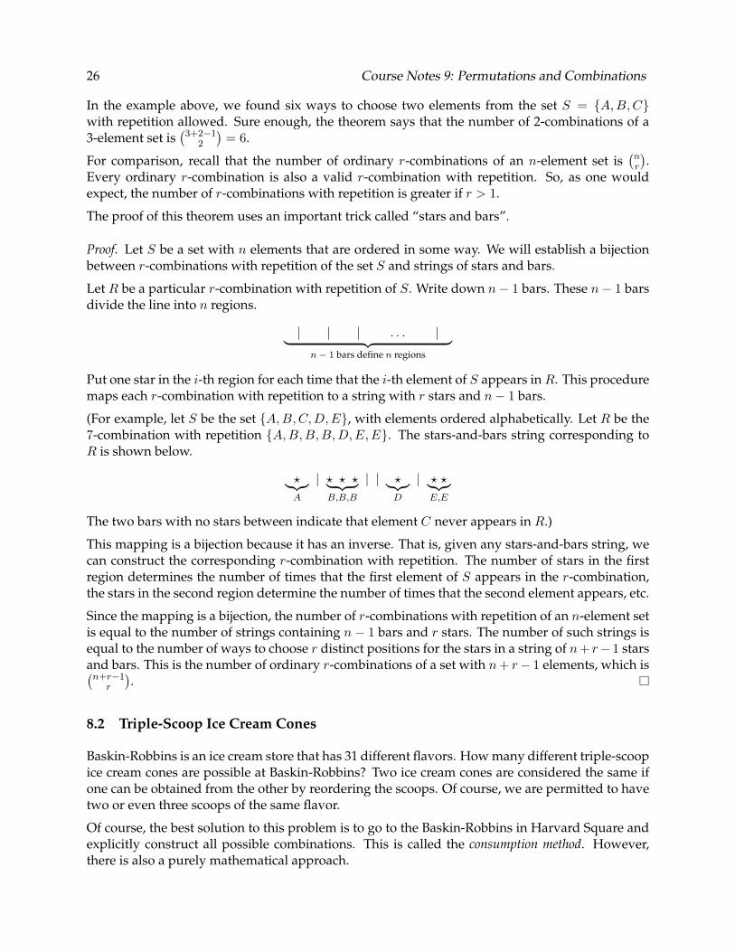
Proof. Let S be a set with n elements that are ordered in some way. We will establish a bijection between r-combinations with repetition of the set S and strings of stars and bars.

Let R be a particular r-combination with repetition of S. Write down n − 1 bars. These n − 1 bars divide the line into n regions.

| | | �� . . . | �

n − 1 bars define n regions

Put one star in the i-th region for each time that the i-th element of S appears in R. This procedure maps each r-combination with repetition to a string with r stars and n − 1 bars.

(For example, let S be the set {A,B, C, D, E}, with elements ordered alphabetically. Let R be the 7-combination with repetition {A,B, B, B, D, E,E}. The stars-and-bars string corresponding to R is shown below.

�� | �� | | �� | � �� A B,B,B D E,E

The two bars with no stars between indicate that element C never appears in R.)

This mapping is a bijection because it has an inverse. That is, given any stars-and-bars string, we can construct the corresponding r-combination with repetition. The number of stars in the first region determines the number of times that the first element of S appears in the r-combination, the stars in the second region determine the number of times that the second element appears, etc.

Since the mapping is a bijection, the number of r-combinations with repetition of an n-element set is equal to the number of strings containing n − 1 bars and r stars. The number of such strings is equal to the number of ways to choose r distinct positions for the stars in a string of n + r − 1 stars and bars. This is the number of ordinary r-combinations of a set with n + r − 1 elements, which is n+r−1 . r

8.2 Triple-Scoop Ice Cream Cones

Baskin-Robbins is an ice cream store that has 31 different flavors. How many different triple-scoop ice cream cones are possible at Baskin-Robbins? Two ice cream cones are considered the same if one can be obtained from the other by reordering the scoops. Of course, we are permitted to have two or even three scoops of the same flavor.

Of course, the best solution to this problem is to go to the Baskin-Robbins in Harvard Square and explicitly construct all possible combinations. This is called the consumption method. However, there is also a purely mathematical approach.

� �

�

� �


The number of triple-scoop ice cream cones is precisely the number of 3-combinations with repetition of the set of 31 flavors. Therefore, we can count the number of ice creams cones with the formula in Theorem 8.1 where n = 31 and r = 3. This gives: �

31 + 3 − 1 �

33 33 · 32 · 31 = = = 5456

3 3 3 · 2 · 1

On Thursdays the Harvard Square Baskin-Robbins is run by an irritating woman who refuses to serve a cone with two or three scoops of the same flavor. How many different triple-scoop ice cream cones are possible on Thursday?

Now we must select an ice cream cone by choosing 3 distinct flavors from the complete set of 31. Therefore, the number of different cones is the number of ordinary 3-combinations of a 31-element set. This is: �

31 31 · 30 · 29 = = 4495

3 3 · 2 · 1

As we would expect, the number of combinations with repetition is greater than number of combinations without repetition. Permitting scoops of the same flavor gives an extra 5456 − 4495 = 961 options.

8.3 Dozens of Dunkin Donuts

Suppose we next stagger down to the Dunkin Donuts in Central Square. We want a box of a dozen doughnuts and there are 21 varieties available. How many options do we have?

We select our box of doughnuts by pointing out 12 varieties from the complete set of 21 where repetition is allowed. Therefore, the number of options is the number of 12-combinations with repetition of a 21 element set. Applying Theorem 8.1 with n = 21 and r = 12, we find that number of different boxes of doughnuts is: �

21 + 12 − 1 �

32 12

=12

= 225, 792, 840

8.4 Balls and Bins

Suppose that we have r identical balls and n distinct bins. In how many ways can we arrange the balls in the bins? There are six possibilities for the case of two balls and three bins, as shown below.

◦ ◦

◦ ◦

◦ ◦

◦ ◦

◦ ◦

◦ ◦

� �

� �

� �

� �

� �

� �

� �

� �

� �


Claim 8.2. There are n+r−1 ways to arrange r identical balls in n distinct bins. r

Proof. Each arrangement of the r balls corresponds to an r-combination with repetition of the set of n bins. Specifically, if the i-th bin contains ai balls, then the corresponding r-combination with repetition contains the i-th bin ai times. Therefore, the number of arrangement of balls is equal to the number of r-combinations of an n-element set, which is n+r−1 by Theorem 8.1. r

There is another way to prove the claim that uses a cute bijection between balls-and-bins arrangements and stars-and-bars strings. The six arrangements in the preceding example are redrawn below with some lines erased and the balls replaced by stars.

Now each balls-and-bin diagram has become a stars-and-bars string. The number of ways to place r balls in n bins is therefore equal to the number of strings with r stars and n − 1 bars, which is

n + r − 1 .

r

8.5 r-Combinations with at Least One of Each Item

Suppose that Kaybee Toys carries balls in three delightful colors: red, blue, and green.3 In how many ways can we choose five balls so that we get at least one ball of each color?

We might as well start by choosing one ball of each color. Then we can choose the last two balls however we like. Remember that we are counting combinations, so the order in which we choose the balls does not matter.

Under this interpretation, the number of options is equal to the number of ways to choose two balls from the set of three colors with repetition allowed. Therefore, by Theorem 8.1 there are�3+2−1

� = 6 possibilities. Here they are:2

{R, G, B, R, R} {R, G, B, R, G} {R, G, B, R, B}{R, G, B, G, G} {R, G, B, G, B} {R, G, B, B,B}

This argument generalizes to give the theorem below. 3I bet you’re wondering if the 6.042 staff has discovered a lucrative scam involving product promotion in lecture

notes. No comment.

� �

� � � �

�

�


Theorem 8.3. The number of r-combinations with repetition of an n-element set that contain every element in the set at least once is:

r − 1 n − 1

For example, in the colored balls problem, we have r = 5 and n = 3. The theorem says that there are

�5−1

� = 6 possibilities, which is consistent with our previous answer.3−1

Proof. Every such r-combination consists of the entire n-element set together with an (r − n)combination with repetition of the n-element set. By Theorem 8.1 the number of such combinations is: � � � � � �

n + (r − n) − 1 r − 1 r − 1 = =

r − n r − n n − 1

m mThe last equality uses the identity k = m−k .

How many n-combinations with repetition� of an n-element set are there that contain every element n−1in the set? In this case, Theorem 8.3 gives n−1 = 1. This makes sense; the only such combination

is the set S itself!

In how many ways can we arrange r identical balls in n distinct bins so that no�bin is empty? �If we� n−1first put one ball in each bin, then we can arrange the remaining r − n balls in n+(r−n)−1 = r−1r−n

ways.

8.6 r-Combinations with Limited Repetition

Suppose that we want to count r-combinations where an element can be repeated only a limited number of times. For example, in how many ways can we arrange 10 identical balls in 4 distinct bins such no bin gets more than 7 balls? A good way to solve such problems is first to count the number of arrangements without a limit on repetition and then to subtract off the illegal arrangements.

The number of ways to arrange 10 identical balls in 4 distinct bins without a limit on repetition is�4+10−1

� = 286.10

Now we must count the illegal arrangements; that is, arrangements in which some bin contains 8 or more balls. Since there are only 10 balls in total, at most one bin can be overloaded with 8 or more balls. We can count the number of ways to overload the first bin by putting 8 balls into the first bin and then observing that the last two balls can be placed in

�4+2−1

� = 10 ways. Since any2

one of the four bins could be overloaded, the total number of illegal arrangement is 4 · 10 = 40.

Overall, there are 286 − 40 = 246 ways to arrange 10 balls in 4 bins so that no bin gets more than 7 balls.

Sometimes when there are limits on repetition, the number of illegal arrangements can itself be difficult to compute. In such cases, a messy inclusion-exclusion calculation may be necessary.

� �

� � �


8.7 Data Compression [Optional]

[Optional]

Stars and bars can help solve a data compression problem. How many bits are needed to specify a multiset of n arbitrary integers in the range [0, 2n]? For example, how much disk space do we need to store one million numbers in the range zero to two million?

A Simple Scheme

One simple scheme is store each number in binary. With this approach, storing each number requires �log2(2n + 1)� bits. Storing all n numbers requires n �log2(2n + 1)� bits. In the case of a million numbers, we need 21 bits to store each number and therefore 21 million bits to store all of the numbers.

A Better Approach Using Stars and Bars

There is a more clever scheme that uses stars and bars. We can regard the multiset of numbers that we want to store as an n-combination with repetition of the (2n + 1)-element set [0, 2n]. The proof of Theorem 8.1 shows that such n-combinations with repetition correspond to strings of n stars and 2n bars. If we represent a star with a 0 and a bar with a 1, then we can store such a stars-and-bars string using n + 2n = 3n bits.

To make the scheme clear, suppose that we are storing a multiset of n = 5 numbers in the range [0, 10]. In particular, suppose that the numbers are {2, 4, 4, 6, 7}. We can represent this multiset as a stars-and-bars string and then with 3n = 15 bits as follows.

{2, 4, 4, 6, 7} → | | � | | � � | | � | � | | | → 1 1 0 1 1 0 0 1 1 0 1 0 1 1 1

As another example, we could store a million numbers in the range zero to two million using only 3 million bits, a factor of 7 improvement over the simple scheme. It is rather surprising that we need only 3 bits per number on average, no matter how large n becomes!

An Optimal Scheme

The stars-and-bars approach is simple and efficient, but not quite optimal.

In any scheme, we must associate every multiset of n numbers with a distinct binary string. From the stars-and-bars interpretation, we know that there are

�3n � possible sets of n numbers. Therefore, we must be prepared to store anyn

one of �3n � distinct binary strings. Using k bits, we can store at most 2k different binary strings. This means that we n �

need at least k bits where 2k ≥ �3n � . This inequality is satisfied provided k ≥ log2

�3n �� . Therefore, as a lower bound,� n n

we need at least log2

�3n �� bits. n

How far from optimal is the stars-and-bars scheme? To answer this question, we must rewrite the lower bound in a more familiar form. To this end, we can use Stirling’s Formula to approximate

�3n � as follows. n

3n (3n)! =

n (2n)! n! � � 3n �3n

2π(3n) e∼ � �

2n �2n √ �

n �n

2π(2n) 2πn e e

3 33n

= 4πn 22n � � �n3 27

= 4πn 4

� � ��

�


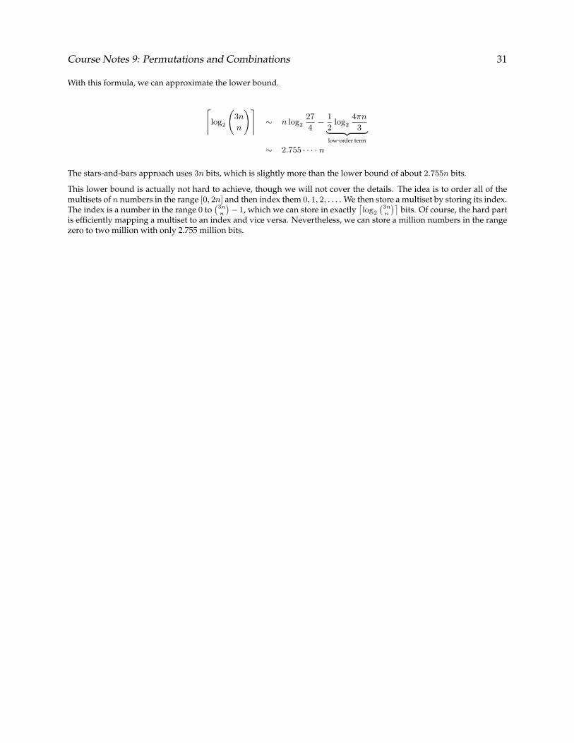
With this formula, we can approximate the lower bound.

3n 27 1 4πn log2 ∼ n log2 −

2 log2 n 4 � �� 3 �

low-order term

∼ 2.755 · · · · n

The stars-and-bars approach uses 3n bits, which is slightly more than the lower bound of about 2.755n bits.

This lower bound is actually not hard to achieve, though we will not cover the details. The idea is to order all of the multisets of n numbers in the range [0, 2n] and then index them 0, 1, 2, . . . . We then store a multiset by storing its index. The index is a number in the range 0 to

�3n � − 1, which we can store in exactly log2

�3n �� bits. Of course, the hard part

n n is efficiently mapping a multiset to an index and vice versa. Nevertheless, we can store a million numbers in the range zero to two million with only 2.755 million bits.

Documents

Permutations and Combinations 1 The Division Rule · 2019-09-12 · 4 Course Notes 9: Permutations and Combinations 2.1 The r-Combinations of a Set Generalizing the example that we