Embed Size (px)
Citation preview
Persistency and Profits’
Biography:
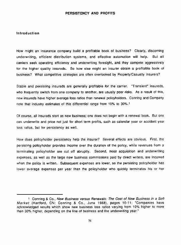
Shalom Feldblum is an Associate Actuary with the Liberty Mutual Insurance Company in Boston, Massachusetts. He was graduated from Harvard University in 1978 and spent the next two years as a visiting fellow at the Hebrew University in Jerusalem. He became a Fellow of the CAS in 1987, a CPCU in 1986, and an Associate of the SOA in 1986. In 1988, while working at the Allstate Research and Planning Center in California, he served as President of the Casualty Actuaries of the Bay Area and as Vice President of Research of the Northern California Chapter of the Society of CPCU. In 1989, he SetV8d on the CAS Education and Testing Methods Task Force, and he is presently a member of the CAS Syllabus Committee. Previous papers and discussions of his have appeared in Best’s Review, the CPCU Journal, the Proceedings of the Casualty Actuarial Society, the Actuarial Digest, the Actuarial Forum, and the CAS Discussion Paper Program.
Abstract:
How can the analysis of persistency patterns aid policy pricing and afford a competitive advantage to the discerning insurer?
When setting rates to optimize long-term income, one should search for policyholders who are price conscious now, who will remain loyal to their insurance carrier, and who will turn profitable in the future. The carrier should offer premium discounts to attract these risks, and then reap the profits later.
Older driver discounts for personal automobile insurance provide a clear illustration of this. Older drivers are loyal to their current insurer, and their average pure premium drops dramatically once they retire. Before they retire, drivers are more price conscious and have higher expected losses.
The carrier should offer a premium discount to attract the driver nearing retirement, before the expected loss ratio actually drops. It will then enjoy the future income from a large and stable population of retiring drivers.
The paper provides an extended demonstration of such pricing techniques. The actuary determines persistency rates and loss ratios by age of the insured and age of the policy. From these he or she calculates the long-term profits expected from premium discounts or surcharges for particular classifications.
The long-term and short-term expected profits may diverge greatly. The rate relativities indicated by short-term “snap-shot” analyses are not necessarily optimal in the long-run. In particular, optimal pricing strategy calls for greater premium discounts for the near- retirement drivers than those indicated by short-term loss ratio analyses.
(’ Laura ShO8 first introduced me to the complexities of the Personal Automobile retired driver discount. Richard Wall taught me that to understand the long-term profitability of a book of business, on8 must examine persistency ratios. I am indebted to both these individuals for stimulating the analysis in this paper.)
PERSISTENCY AND PROFITS
Introduction
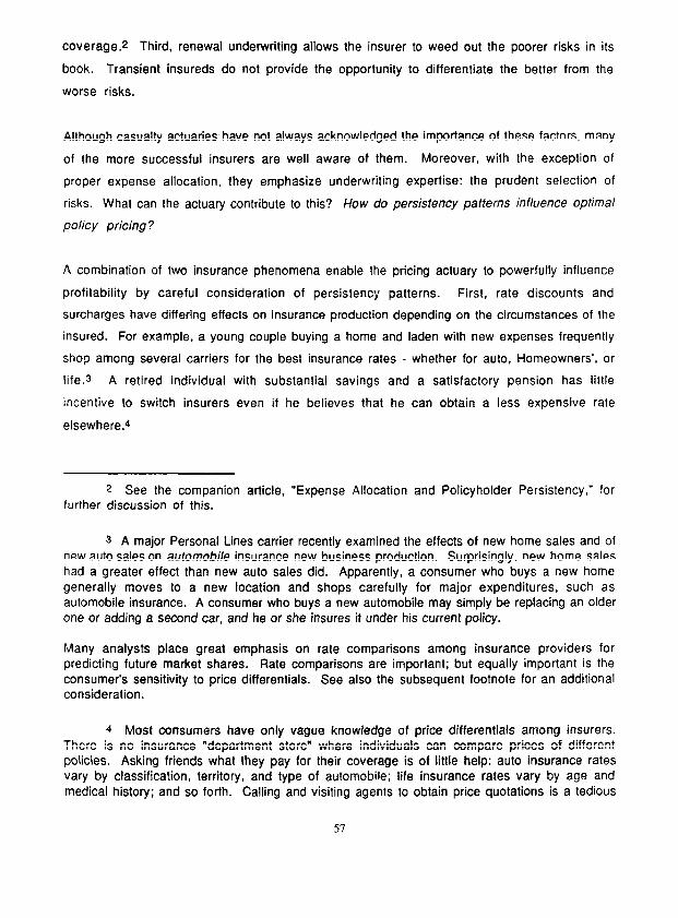
How might an insurance company build a profitable book of business? Clearly, discerning
underwriting, efficient distribution systems, and effective automation will help. But all
carriers seek operating efficiency and underwriting foresight, and they compete aggressively
for the higher quality insureds. So how else might an insurer obtain a profitable book of
business? What competitive strategies are often overlooked by Property/Casualty insurers?
Stable and persisting insureds are generally profitable for the carrier. “Transient” insured&
who frequently switch from one company to another, are usually poor risks. As a result of this,
new insureds have higher average loss ratios than renewal policyholders. Conning and Company
note that industry estimates of this differential range from 10% to 30%.1
Of course, all insureds start as new business; one does not begin with a renewal book. But one
can underwrite and price not just for short term profits, such as calendar year or accident year
loss ratios, but for persistency as well.
How does policyholder persistency help the insurer? Several effects are obvious. First, the
persisting policyholder provides income over the duration of the policy, while revenues from a
terminating policyholder are cut off abruptly. Second, most acquisition and underwriting
expenses, as well as the large new business commissions paid by direct writers, are incurred
when the policy is written. Subsequent expenses are lower, so the persisting policyholder has
lower average expenses per year than the policyholder who quickly terminates his or her
1 Conning 8 Co., New Business versus Renewals: The Cost of New Business in a Soft Market (Hartford, CN: Conning & Co., June 1988), pages IO-II: “Companies have acknowledged results which show new business loss ratios varying from 10% higher to more than 30% higher, depending on the line of business and the underwriting year.”
coverage.* Third, renewal underwriting allows the insurer to weed out the poorer risks in its
book. Transient insureds do not provide the opportunity to differentiate the better from the
worse risks.
Although casualty actuaries have not always acknowledged the importance of these factors, many
of the more successful insurers are well aware of them. Moreover, with the exception of
proper expense allocation, they emphasize underwriting expertise: the prudent selection of
risks. What can the actuary contribute to this ? How do persistency patterns influence optimal
policy pricing ?
A combination of two insurance phenomena enable the pricing actuary to powerfully influence
profitability by careful consideration of persistency patterns. First, rate discounts and
surcharges have differing effects on insurance production depending on the circumstances of the
insured. For example, a young couple buying a home and laden with new expenses frequently
shop among several carriers for the best insurance rates - ‘whether for auto, Homeowners’, or
life.3 A retired individual with substantial savings and a satisfactory pension has little
incentive to switch insurers even if he believes that he can obtain a less expensive rate
elsewhere.4
* See the companion article, “Expense Allocation and Policyholder Persistency,” for further discussion of this.
3 A major Personal Lines carrier recently examined the effects of new home sales and of new auto sales on automobile insurance new business production. Surprisingly, new home sales had a greater effect than new auto sales did. Apparently, a consumer who buys a new home generally moves to a new location and shops carefully for major expenditures, such as automobile insurance. A consumer who buys a new automobile may simply be replacing an older one or adding a second car, and he or she insures it under his current policy.
Many analysts place great emphasis on rate comparisons among insurance providers for predicting future market shares. Rate comparisons are important; but equally important is the consumer’s sensitivity to price differentials. See also the subsequent footnote for an additional consideration.
4 Most consumers have only vague knowledge of price differentials among insurers. There is no insurance “department store” where individuals can compare prices of different policies. Asking friends what they pay for their coverage is of little help: auto insurance rates vary by classification, territory, and type of automobile; life insurance rates vary by age and medical history; and so forth. Calling and visiting agents to obtain price quotations is a tedious
57
Second, average loss costs vary over the life of a policy. For example, many young unmarried
men are carefree drivers, less concerned with safety than with presenting a courageous image.
Once they have married, begun careers, and borne children, they feel more responsibility, both
individual and financial, for their families - and their driving habits improve accordingly.
When their children become adolescents and start driving the family cars, auto insurance loss
costs climb rapidly. But when the children leave home and the insured retires, the automobiles
may be unused except for shopping trips and weekend vacations; automobile accidents become
rare. Finally, when the driver enters his or her 70’s, physiological health deteriorates and
reactions are slowed. If the insured continues to drive, accident frequency increases.
For certain coverages, premium discounts and surcharges have a strong effect on sales when the
insured is an average risk. But when the insured’s “risk qualities” improve, rate relativities
have less influence on either new business production or policyholder persistency. An effective
competitive strategy is to provide premium discounts to persisting policyholders when price
has a strong effect on sales, and reap the profits later when risk quality improves but price
sensitivity decreases.
The theory sounds fine - but are there practical uses for this? Indeed, there are many: a clear
example is the older driver discount for automobile insurance. First, however, we take a slight
detour, to examine the influences on price elasticity of demand for insurance. What causes
policyholders to terminate or renew their coverage?
process, practiced by few individuals.
Thus, one must consider the consumer’s knowledge of price differentials, in addition to his sensitivity to price differentials. Besides a lower sensitivity, a retired insured has less knowledge of insurance rates. Other individuals may discuss auto insurance rates at work or over lunch; the retired driver often lacks these opportunities. For further discussion of these issues, see Paul L. Joskow, “Cartels, Competition, and Regulation in the Property-Liability Insurance Industry,” The Bell Journal of Economics and Management Science, Vol. 4, No. 2 (Autumn 1973) pages 375-427, and Sholom Feldblum, “How Competitive is the P/C Industry?” Best’s Review: Property/Casualty Edition, Vol. 88, No. 10 (February 1988) pages 14 ff.
58
Price Elasticity of Demand for Insurance
When purchasing fruit at a corner grocery store, or filling up the car at a gas station, a
consumer may select the supplier based on penny differences. Yet while vacationing overseas,
the same individual may expend hundreds of dollars for a fancier hotel. In other words, price
elasticity of demand for a particular brand is high when purchasing staples, but low when
purchasing a luxury. What about the purchase of Personal Automobile insurance: is price
elasticity high or low?
In general three factors influence price elasticity: the nature of the product, the availability of
substitute goods, and the current price of the product.
1. The nature of the product: Essential goods, such as food staples, infants’ clothes, and gas
prices, are relatively inelastic. A small change in price has little effect on quantity demanded,
since people must eat food, wear clothing, and drive to work in any case. Luxury goods, such as
jewelry, restaurant meals, and airline travel, are relatively elastic. The consumer freely
chooses whether or not to purchase the product, and price changes may influence this decision.5
2. The availability of substitute products: Price elasticity increases when substitute products
are more readily available. The demand for bus tickets is relatively inelastic if buses are the
only means of public transportation. If commuter trains and airlines travel along the same
routes, the demand for bus tickets is more elastic.6
3. The current price of the product: Elasticity differs as one moves along the demand curve. If
the current price is very low, consumption may be near its maximum. A further price
reduction may have little effect on quantity demanded. If the current price is very high,
5 This paragraph discusses aggregate price elasticity of demand for the industry’s product. The comments in the first paragraph of this section, on purchasing decisions for gas and hotels, relate to price elasticity of demand for a given supplier’s product. These two elasticities are often inversely related; see below in the text.
s Hal Ft. Varian, intermediate Microeconomics: A Modern Approach (New York: W. W. Norton & Co., 1987), page 275, emphasizes this: “The elasticity of demand for a good depends to a large extent on how many close substitutes it has.”
59
consumption may be near its minimum. The same percentage price reduction would have a much
larger effect on the quantity demanded.7
Industry and Firm Price Elasticities
This price elasticity refers to the industry-wide demand, not the demand for a particular firm’s
output. In fact, elementary economic theory has little place for an individual firm’s price
elasticity. In monopolies, there is no difference between the individual firm and the industry.
In competitive industries, economists assume that firms are price takers. If a firm raises
prices unilaterally, it loses all its market share. Price elasticity for firms in purely
competitive industries is infinite.8
Only in the nebulous realm of imperfect competition is price elasticity for individual firms a
meaningful concept.9 Different factors, however, influence elasticity for the firm: product
differentiation, switching costs, and the extent of price shopping.10
1. Product differentiation: The more a firm differentiates its products, the more it can raise
7 The effect of the current price on the elasticity depends on the shape of the demand curve. See J. M. Henderson and R. E. Quandt, Microeconomic Theory: A Mathematical Approach, Third Edition (New York: McGraw-Hill, 1980) for a mathematical treatment of this.
s See, for example, Paul A. Samuelson, Economics, 1 Ith edition (New York: McGraw-Hill, 1980). p. 430: “A perfect-competitor is too small and unimportant to affect the market price. , . , In terms of demand elasticity, a perfect-competitor faces a (virtually) horizontal dd demand curve for its product - its elasticity of demand is infinite.”
9 Edwin Mansfield, Microeconomics (New York: W. W. Norton 8 Co., 1975), pages 303- 304, illustrates this with two demand curves for a firm. One shows “how much the firm will sell if it varies its price from the going level and if other firms maintain their existing prices.” The other demand curve is “based on the proposition that a// firms raise or lower their prices by the same amount as this firm.”
10 For an extensive treatment of these factors, see Michael Porter, Competitive Strategy (New York: The Free Press, 1980). Porter examines the competitive characteristics of the industry, not the just price elasticity of demand for the product, so he includes other items in his analysis as well.
60
prices without losing customers. Conversely, if consumers perceive little difference among
various firms’ products, price changes by any one firm cause large market share changes.11
Among automobile insurance policies, there is little product differentiation, so we would expect
high price elasticity.
2. Switching costs: Switching suppliers may be expensive, even when products are similar.
Additional expenses include installation costs, inspection costs, training costs, and adaptation
costs. These expenses are particularly important for new parts in a manufacturing plant.12
There are almost no switching costs for the automobile insured, so we would again expect high
price elasticity.
3. Extent of price shopping: The more price shopping consumers do, the less likely are firms to
raise prices unilaterally. The more that non-price factors influence consumers’ purchases, the
more flexibility suppliers have to adjust prices.
Buyers of new automobile polices sometimes compare prices carefully. At renewal time,
however, most insureds do not price shop, unless they believe that their policy is substantially
overpriced. In other words, we would expect high price elasticity for new policyholders but low
price elasticity for renewal policyholders.
In general, there is an inverse relationship between demand elasticity for the industry and for
the individual firm. For commodities, industry demand is inelastic, since consumers demand
the product regardless of small or even moderate price changes. However, such products are
rt Product differentiation creates two goods that are close substitutes. The cross elasticity of demand measures the effect of price changes of one good on demand for the other. See Evan J. Douglas, intermediate Microeconomic Analysis: Theory and Applications (Englewood Cliffs, NJ: Prentice-Hall, Inc., 1982), pages 9598.
12 Michael Porter, Competitive Strategy (New York: The Free Press, 1980), defines switching costs as “one-time costs facing the buyer of switching from one supplier’s product to another’s” (p. IO), and he adds: “Switching costs may include employee retraining costs, cost of new ancillary equipment, cost and time in testing or qualifying a new source, need for technical help as a result of reliance on seller engineering aid, product redesign, or even psychic costs of severing a relationship.”
61
usually undifferentiated, switching costs are low, and consumers aggressively compare
competitors’ prices. Thus, the firm’s demand is elastic.
For luxury items, industry demand is elastic. However, these products are highly
differentiated, switching costs may be large, and consumers tend to stick with a particular
supplier. Thus, the firm’s demand is inelastic.
Personal Automobile Price Elasticity
For automobile insurance, industry-wide consumer demand is inelastic. Financial
Responsibility statutes and compulsory insurance legislation make insurance coverage
essential. Drivers complain when rates increase, but they rarely reduce liability limits to save
money. Moreover, product differentiation among automobile insurance policies is insignificant,
and drivers are often unaware of the differences that do exist among policies.13
Automobile insurance is about as close as a complex commercial product can get to a commodity.
Thus, we would expect the price elasticity for the individual firm to be quite high.
Reality shows the opposite. If price elasticity for the individual firm were high, we would not
13 See, for instance, William A. Sherdan, “An Analysis of the Determinants of Demand for Automobile Insurance,” The Journal of Risk and Insurance, Volume 51, No. 1 (March 1984), page 58: “Bodily injury coverage is highly insensitive to price and is price-inelastic even at price levels twice the state average price.” Sherdan ascribes the price inelasticity to “the substantial risks associated with owning and operating a vehicle” (page 50), not to state statutes or regulations. This is surprising, since he uses data from Massachusetts, a compulsory insurance state.
Thomas S. Bloom, “Cycles and Solutions,” Best’s Review: Property/Casualty Edition, Volume 86, No. 6 (October 1987), page 21, lists four factors contributing to the low elasticity of demand for insurance:
“(1) Much of the coverage is purchased because it is required by law. (2) Much of the coverage is purchased because it is required by a lender. (3) The product is relatively essential and is recognized as such by most buyers. (4) The product is not purchased in duplicate. No matter how low prices go, the
individual will buy only one homeowners policy, the corporation will buy only one workers’ compensation contract.
These facts combine to make the demand curve inelastic.”
62
expect large price differences for the same insured from different insurers. Yet the rate
charged by one insurer may be twice that charged by another company for the same risk.14
The experience of the major Personal Automobile direct writers demonstrates the difference
between renewal and new policyholders. Overall renewal ratios in most states are about 90%.
Rate revisions have little effect on termination rates: a rate hike of lo-15% lowers renewal
ratios by only l-2%. In other words, price elasticity of demand is extremely low for existing
policyholders.1 s
The converse is true for new insureds. Many new insureds are seeking low premiums, and a
lo-15% rate hike may cut new insurance production by an equal percentage. In other words,
demand for auto insurance is elastic for new policyholdersls
What causes this great disparity between existing and new policyholders? Elasticity of demand
measures the influence of price upon the actions of the consumer. For most goods, the purchase
of the item is the action. For instance, when a driver needs gas, the action is stopping at a gas
station and filling up the tank. When a consumer buys food, the action is entering a grocery
store or supermarket and selecting various items.
14 See “Auto Insurance,” Consumers Reporfs (October 1988) pages 622-636. The authors provide the following illustration: “A husband and wife and their 17-year old son, each have a clean traffic record. They own a 1987 Buick LaSabre, used to commute to work, and a 1985 Chevrolet Cavalier. If they lived in San Francisco, they might pay as much as $4,248 a year to insure their cars - or as little as $2,022 for identical coverage. In Manhattan, their premiums might be as high as $4,806 or as low as $2,553: in Chicago, as high as $2,976 or as low as $1,516” (page 630).
1s Demand for Commercial Lines insurance products is more price elastic, since large insureds have various risk management alternatives to standard insurance coverage. Moreover, business risk managers often carefully compare policy prices at renewal dates - which Personal Lines consumers rarely do.
1s There are few published studies of price elasticity for insurance. The various legal requirements mandating coverage, such as Financial Responsibility Laws and compulsory insurance statutes, and the diversity of Property-Casualty insurers, make such analyses difficult. Private studies, using data from a major Personal Lines carrier, show price elasticities of demand for the individual firm between -0.10 and -0.15 for existing policyholders and between -1 and -2 for new business. These figures vary with the distribution system used by the insurer and with the competitive characteristics of the marketplace, and so they should not be generalized to other insurance companies.
63
This is not the case for insurance. The policyholder receives a renewal bill, writes a check, and
mails it to the insurer. Renewing the policy is the path of least resistance. Terminating the
policy, however, may be an arduous task. The policyholder must seek out another agent, visit
his or her office, fill out an application, and wait for the issue of the policy.
Thus, when examining elasticity of demand, we must measure the influence of price upon
production rates for new business and upon termination rates for existing policyholders.
Overall termination rates are about 10% for the major direct writers. A rate hike of 10-l 5%
will increase the termination rate to about 11 or 12% - which makes sense for an
undifferentiated product in a competitive market.1 7
Price elasticity of demand is one of the determinants of persistency patterns, which influence
long-term profits and optimal rate relativities. Since rate revisions change persistency
patterns, their effect on long-term profits may differ from their effect on short-term income.
This phenomenon is described in detail in the remainder of the paper.
17 Automobile insurance may be compared to durable goods, such as autos, freezers, and washing machines, though the similarity is imperfect. The consumer purchases the good at a specific date, but he or she uses it over the next several years. If the durable good is financed by a car loan or by a credit card, the consumer may pay for it over the next several years as well.
Comparison shopping occurs at the date of purchase, not over the life of the good. Even though the cost of the good may be “capitalized” by means of a consumer loan, and the purchase expense is spread over several years, elasticity of demand depends upon conditions only at the date of sale.
Automobile insurance is similar. The issue of a new policy corresponds to the date of sale, while the payment of renewal premiums corresponds to the periodic cash expenditures for a consumer loan. The degree of similarity, of course, depends on the loyalty of the policyholder to the insurer. The lower the termination rates, the more similar is automobile insurance to durable goods.
As noted above, the similarity is imperfect. The payments for a durable good are fixed at the time of sale. Renewal payments for insurance coverage vary with the insurer’s rate changes. Changing “suppliers” during the lifetime of the durable good is expensive, even if the consumer can trade in the old item for a partial reduction in price. Changing insurers at the renewal date may be onerous, but it is not expensive.
64
Retired Drlver Discounts
Anecdotes abound about the poor reflexes and slow responses of older drivers. Before good data
were available, auto insurers surcharged older insureds, since they expected them to have
higher accident frequencies. Insurance experience shows the opposite, apparently for two
reasons. First, older individuals, particularly if they are retired, drive less often and for
shorter distances.18 Second, many older drivers, aware of their physical limitations, drive
more carefully and more slowly than younger drivers do. Knowing that they can not easily
escape dangers once they arise, they tend to avoid dangerous situations in the first place.19
1s C. A. Kulp and John W. Hall, Casualty insurance (New York: John Wiley and SOnS, 1968), page 390, show the effect of driving to work on Personal Automobile insurance rates in a widely used (1967) classification scheme. An adult who drives a vehicle 10 or more miles to work each day pays a premium 40% higher than if he or she used the auto for pleasure only.
Although mileage driven is a major influence on the low loss costs of retired drivers, it is difficult to objectively ascertain and so is a poor classification dimension. See Paul Dorweiler, “Notes on Exposure and Premium Bases,” Proceedings of the Casualty Actuarial Society, Volume 16 (1929-30), page 338, [reprinted in Volume 58 (1971), page 781: “The mileage exposure medium is superior to the car-year medium in yielding an exposure that varies with the hazard, as it responds more to the actual usage of the car. The devices and records necessary for the introduction of this medium make it impractical under present conditions.”
19 See Ambrose Ryder, “Informal Discussion: Automobile Liability Insurance,” Proceedings of the Casualty Actuarial Society, Volume 22 (1935-36), page 143:
“The next question is whether a driver is a better risk because he reacts one-fifth of a second quicker than the average. Various devices have been on the market for testing the reaction times to danger signals. I think these are all very interesting and may possibly prove of value, but generally speaking the person who is quick on the trigger and who reacts very promptly is probably a less desirable risk than the more phlegmatic person who likes to think things over two or three times before he decides to do anything. The latter type will not react as quickly to the sudden danger that presents itself to his oncoming car but on the other hand neither will he be so likely to allow himself to get into a position where any sudden danger will arise that will require a one-tenth of a second reaction. Give me my choice and I will take the man who is not so quick on the trigger in everything he does in life.
“If the individual driver is going to be measured for his reactions to danger, it is even more important that he should be measured for his willingness to keep away from danger. In other words, although courage is a splendid attribute in its place, its place is not at the wheel of an automobile. The timid soul is a much better risk that the daring young man who has the courage to drive his car at 90 miles per hour on a slippery road. The best type of risk, therefore, is the
65
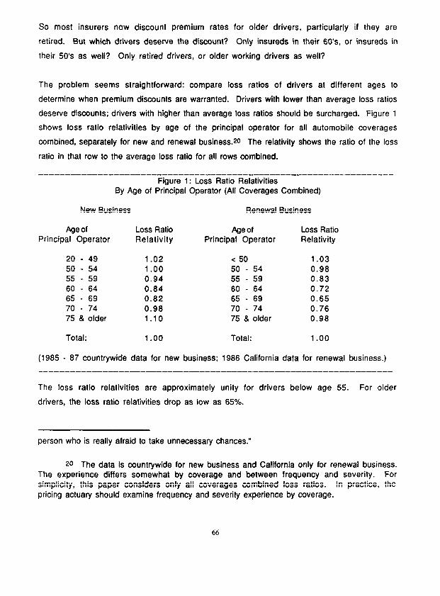
So most insurers now discount premium rates for older drivers, particularly if they are
retired. But which drivers deserve the discount? Only insureds in their 60’s, or insureds in
their 50’s as well? Only retired drivers, or older working drivers as well?
The problem seems straightforward: compare loss ratios of drivers at different ages to
determine when premium discotints are warranted. Drivers with lower than average loss ratios
deserve discounts; drivers with higher than average loss ratios should be surcharged. Figure 1
shows loss ratio relativities by age of the principal operator for all automobile coverages
combined, separately for new and renewal business.20 The relativity shows the ratio of the loss
ratio in that row to the average loss ratio for all rows combined.
-------------_---------------------------------------------------- Figure 1: Loss Ratio Relativities
By Age of Principal Operator (All Coverages Combined)
New Business Renewal Business
Age of Principal Operator
20 - 49 50 - 54 55 - 59 60 - 64 65 - 69 70 - 74 75 8 older
Loss Ratio Relativity
1.02 1 .oo 0.94 0.84 0.82 0.98 1 .lO
Age of Loss Ratio Principal Operator Relativity
< 50 1.03 50 - 54 0.98 55 - 59 0.83 60 - 64 0.72 65 - 69 0.65 70 - 74 0.76 75 & older 0.98
Total: 1.00 Total: 1 .oo
(1985 - 87 countrywide data for new business: 1986 California data for renewal business.)
The loss ratio relativities are approximately unity for drivers below age 55. For older
drivers, the loss ratio relativities drop as low as 65%.
person who is really afraid to take unnecessary chances.”
so The data is countrywide for new business and California only for renewal business. The experience differs somewhat by coverage and between frequency and severity. For simplicity, this paper considers only all coverages combined loss ratios. In practice, the pricing actuary should examine frequency and severity experience by coverage.
66
The loss ratio differences are more pronounced for existing policyholders than for new
insureds. For new business, the loss ratio relativities never dip below 82%. The loss ratio
relativities for renewal policyholders are at or below this level from age 55 through 74.
This difference makes sense, since the effects of aging differ among insureds. Some retired
drivers drive less and drive more carefully; these are the best risks. Others find their
responses dulled, but do not change their driving habits; these are dangerous insureds.
Why would a 65 year old individual be looking for a new auto insurance policy? Many retired
persons own their own homes and have close friends in their neighborhoods. They are not
inclined to move elsewhere and begin new lives or careers - the most common motive for
switching insurers. Those who do move often do so because of failing health. They join
retirement communities, enter old age homes, or live with their children. They are not usually
seeking new auto policies.
Insurers frequently review the policies of drivers who have had recent accidents. If the insurer
believes the driver is too risky, it may terminate the policy or “discourage” renewal (e.g., by
indifferent customer service). Some of the retired drivers seeking new automobile insurance
policies have been considered poor risks by their former insurers.
Exposure distributions by age of the principal operator for new and renewal business show this
clearly. Among existing policyholders, older drivers form a large percentage of the population
and are generally good risks. Among new insureds, older drivers form a smaller percentage of
the population. Some of these insureds are good risks; others are dangerous drivers.
67
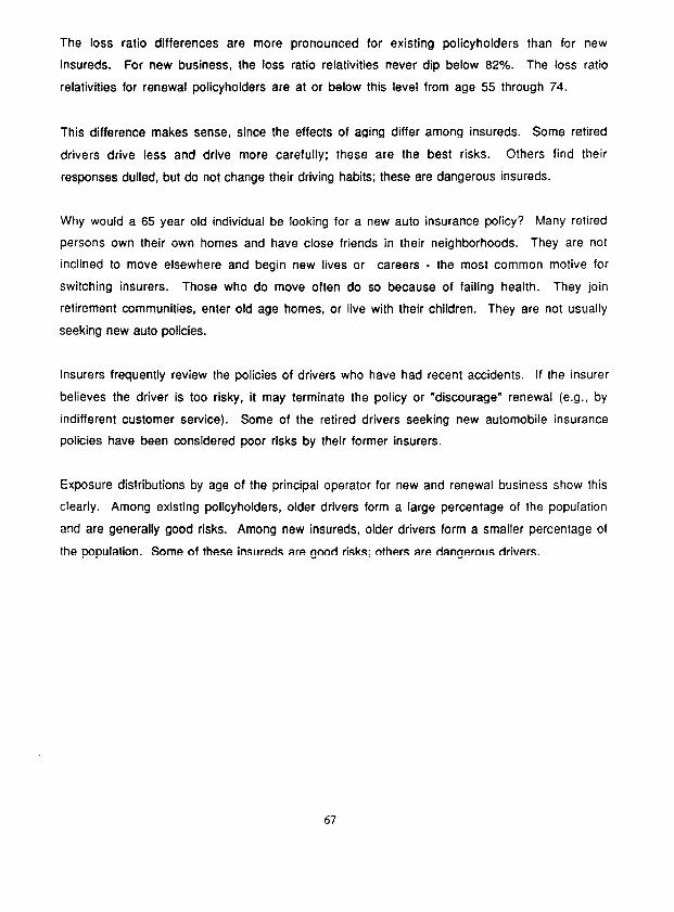
Figure 2 shows exposure distributions for the insureds in Figure 1. Note that insureds age 50
and over form 29% of the renewal business but only 23% of the new business.
_~__-----------_--------~--------------~~-----~~~~~--~~~~---~~~~~~ Figure 2: Exposure Distribution
By Age of Principal Operator
New Business Renewal Business
Age of Principal Operator
Exposure Distribution
Ageof Principal Operator
Exposure Distribution
20 - 49 76.7% < 50 70.9% 50 - 54 5.8 50 - 54 7.2 55 - 59 5.2 55 - 59 6.4 60 - 64 4.6 60 - 64 5.8 65 - 69 3.3 65 - 69 4.1 70 - 74 2.4 70 - 74 2.9 75 & older 2.0 75 & older 2.7
Total: 100.0% Total: 100.0%
(1985 - 87 countrywide data for new business: 1986 California data for renewal business.)
Finally, retired drivers have lower loss ratios than working insureds among the 50 and over
population: 75.6% for the retired drivers versus 83.4% for non-retired older drivers in the
1986 California experience (existing policyholders).21
These figures are consistent, and the conclusion is clear. The older driver discount is warranted
after age 55, not before. And it is deserved primarily by retired drivers, not by those still
working.
21 For differentiating between loss ratios of retired and other drivers, we examined the experience only for drivers aged 50 and above. Few individuals below age 50 are retired. These younger drivers had higher loss ratios in the California experience, and they brought the overall loss ratio among non-retired drivers to 92.5%.
68
Persistency Patterns
But this conclusion is incorrect, for we asked the wrong question. We asked, “Which drivers
deserve premium discount? At what age are premium discounts warranted?”
Were there no competition among insurers, these questions would be appropriate. If all
insurers adhered to rating bureau prices, the pricing actuary at the bureau should indeed ask
such questions.
But the private insurer asks, “What type of premium discount will maximize my long-term
profits and enlarge my market share. 3” Loss ratio comparisons are like snapshots. They show
the profits in a particular span of time. When used alone, they do not tell you what the
long-term results will be. They must be combined with persistency patterns to produce
meaningful results.
Termination rates vary dramatically by risk classification. Young unmarried male drivers
have policy termination rates as high as 20-30%, since they frequently move to other
locations, sell their automobiles and acquire new ones, or get married and switch to their wives’
insurers.22 Retired drivers in their 60’s and 70’s have termination rates as low as 3 or 4%,
since they have little incentive or stamina for comparison shopping.
Figure 3 shows voluntary termination rates for new business by age of the principal operator.
The overall rates are quite high, since most policy terminations occur on new business. (If one
adds an additional point or two for underwriting terminations, or “involuntary” terminations,
the overall rate equals the first renewal termination rate shown in Figure 4.) Figure 3 shows
that older insureds are less likely to terminate their policies than other insureds are. We will
use the termination relativities below to estimate termination rates for an existing older
driver.
22 See the companion article, “Expense Allocation and Policyholder Persistency,” for termination rates among young male drivers. Termination rates are particularly high when there is frequent public debate about premium costs, such as in California during the insurance initiative campaigns of 1988. They are low when rate quotations from competing carriers are difficult to obtain, such as in sparsely populated rural areas.
69
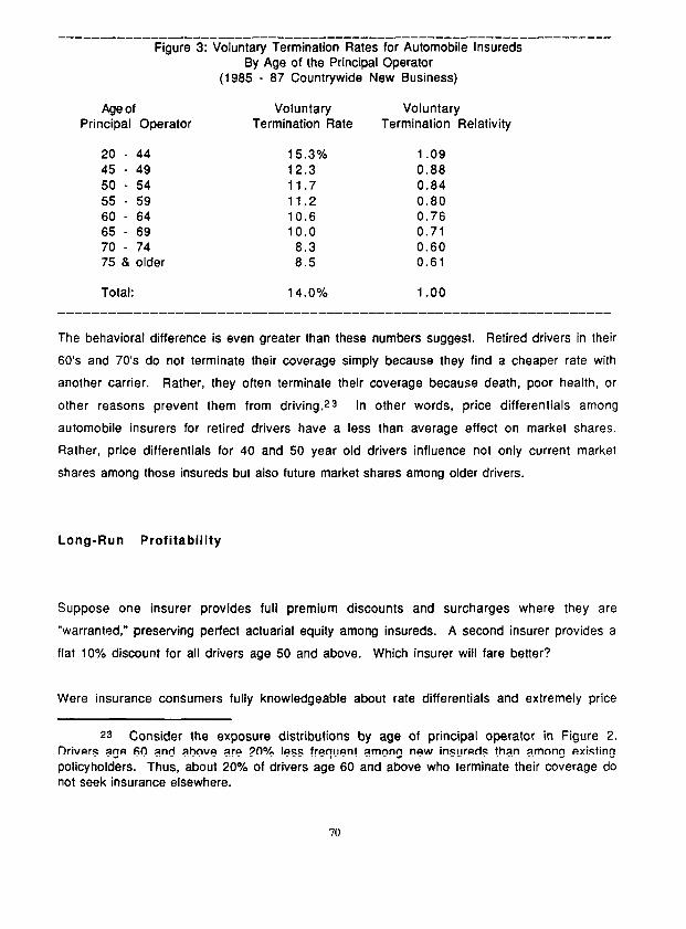
Figure 3: Voluntary Termination Rates for Automobile lnsureds By Age of the Principal Operator
(1985 - 87 Countrywide New Business)
Age of Principal Operator
Voluntary Voluntary Termination Rate Termination Relativity
20 - 44 15.3% 1.09 45 - 49 12.3 0.88 50 - 54 11.7 0.84 55 - 59 11.2 0.80 60 - 64 10.6 0.76 65 - 69 10.0 0.71 70 - 74 8.3 0.60 75 & older 8.5 0.61
Total: 14.0% 1 .oo
The behavioral difference is even greater than these numbers suggest. Retired drivers in their
60’s and 70’s do not terminate their coverage simply because they find a cheaper rate with
another carrier. Rather, they often terminate their coverage because death, poor health, or
other reasons prevent them from driving.23 In other words, price differentials among
automobile insurers for retired drivers have a less than average effect on market shares.
Rather, price differentials for 40 and 50 year old drivers influence not only current market
shares among those insureds but also future market shares among older drivers.
Long-Run Profitability
Suppose one insurer provides full premium discounts and surcharges where they are
“warranted,” preserving perfect actuarial equity among insureds. A second insurer provides a
flat 10% discount for all drivers age 50 and above. Which insurer will fare better?
Were insurance consumers fully knowledgeable about rate differentials and extremely price
2s Consider the exposure distributions by age of principal operator in Figure 2. Drivers age 60 and above are 20% less frequent among new insureds than among existing policyholders. Thus, about 20% of drivers age 60 and above who terminate their coverage do not seek insurance elsewhere.
70
conscious, the second insurer would do poorly. Among insureds age 50 to 54, it would earn IeSS
than its desired return. Once insureds turned 55, they would switch to the first insurer, which
has larger premium discounts for these drivers.
In the real world, the second insurer would thrive. Among insureds age 50 to 54, it would
indeed earn less than it wanted, but it would build up market share. These insureds will stay
with it for the coming years, when the mere 10% discount makes them profitable for the
carrier.
How well would the second insurer do? Consider an existing policyholder aged 52, the midpoint
of the 50-54 age group. We know his expected loss ratio relativity from Figure 1. To
determine the long-term expected profits for the insurer, we must estimate this policyholder’s
expected persistency.24
Termination Rates
Termination rates vary by policy duration even more than they do by classification. Most
insureds terminate their policies within a year or two after issue - perhaps they are unhappy
with the service, or they have been looking around for a better premium rate.
24 The loss ratios, persistency patterns, and retativities in this paper are rough figures. Most numbers are for 5 year age groups, though the variance from year to year is significant. This paper demonstrates pricing methods; it does not seek to determine the optimal rate relativity for an older driver. Since persistency patterns vary among insurers, the pricing actuary must examine renewal and termination rates in his own book of business or in companies with similar operating characteristics.
71
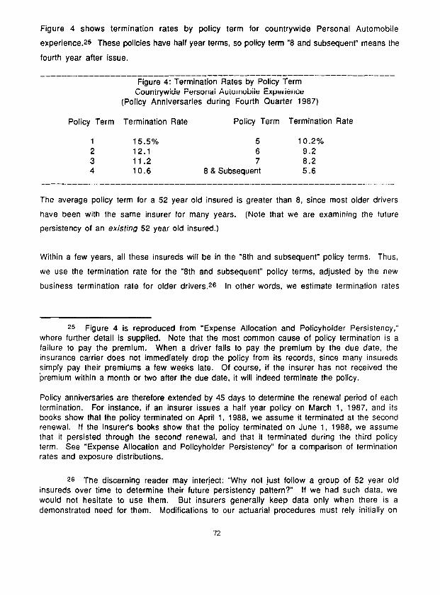
Figure 4 shows termination rates by policy term for countrywide Personal Automobile
experience.25 These policies have half year terms, so policy term “8 and subsequent” means the
fourth year after issue.
__--------_-----_-------~~~~~--~~------~~~~---~~~~~~-~~~~--------- Figure 4: Termination Rates by Policy Term
Countrywide Personal Automobile Experience (Policy Anniversaries during Fourth Quarter 1987)
Policy Term Termination Rate Policy Term Termination Rate
1 15.5% 5 10.2% 2 12.1 6 9.2 3 11.2 7 8.2 4 10.6 8 & Subsequent 5.6
The average policy term for a 52 year old insured is greater than 8, since most older drivers
have been with the same insurer for many years. (Note that we are examining the future
persistency of an existing 52 year old insured.)
Within a few years, all these insureds will be in the “8th and subsequent” policy terms. Thus,
we use the termination rate for the “8th and subsequent” policy terms, adjusted by the new
business termination rate for older drivers .se In other words, we estimate termination rates
25 Figure 4 is reproduced from “Expense Allocation and Policyholder Persistency,” where further detail is supplied. Note that the most common cause of policy termination is a failure to pay the premium. When a driver fails to pay the premium by the due date, the insurance carrier does not immediately drop the policy from its records, since many insureds simply pay their premiums a few weeks late. Of course, if the insurer has not received the premium within a month or two after the due date, it will indeed terminate the policy.
Policy anniversaries are therefore extended by 45 days to determine the renewal period of each termination. For instance, if an insurer issues a half year policy on March 1, 1987, and its books show that the policy terminated on April 1, 1988, we assume it terminated at the second renewal. If the insurer’s books show that the policy terminated on June 1, 1988, we assume that it persisted through the second renewal, and that it terminated during the third policy term. See “Expense Allocation and Policyholder Persistency” for a comparison of termination rates and exposure distributions.
2s The discerning reader may interject: “Why not just follow a group of 52 year old insureds over time to determine their future persistency pattern?” If we had such data, we would not hesitate to use them. But insurers generally keep data only when there is a demonstrated need for them. Modifications to our actuarial procedures must rely initially on
72
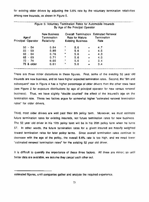
for existing older drivers by adjusting the 5.6% rate by the voluntary termination relativities
among new insureds, as shown in Figure 5.
-~____---__-----__------------~--------------------~~---~~~~~~~~~- Figure 5: Voluntary Termination Rates for Automobile lnsureds
By-Age of the Principal Operator
Age of Principal Operator
New Business Termination Relativity
Overall Termination Estimated Renewal Rate for Mature Termination
Existing Business Rate
50 - 54 0.84 l 5.6 = 4.7 55 59 l - 0.80 5.6 = 4.5 60 l - 64 0.76 5.6 = 4.3 65 l - 69 0.71 5.6 = 4.0 70 74 0.60 * - 5.6 = 3.4 75 & older 0.61 l 5.6 = 3.4
There are three minor distortions in these figures. First, some of the existing 52 year old
insureds are new business, and so have higher expected termination rates. Second, the “8th and
subsequent” row in Figure 4 has a higher percentage of older drivers than the other rows have
(see Figure 2 for exposure distributions by age of principal operator for new versus renewal
business). Thus, we have slightly “double counted” the effect of the insured’s age on the
termination rate. These two factors argue for somewhat higher “estimated renewal termination
rates” for older drivers.
Third, most older drivers are well past their 8th policy term. Moreover, we must estimate
future termination rates for existing insureds, not future termination rates for new business.
The 52 year old driver in his 10th policy term will be in his 20th policy term when he turns
57. In other words, the future termination rates for a given insured are heavily weighted
toward termination rates for later policy terms. Since overall termination rates continue to
decrease with the age of the policy, the overall 5.6% rate is too high, and we need lower
“estimated renewal termination rates” for the existing 52 year old driver.
It is difficult to quantify the importance of these three factors. All three are minor; so until
better data are available, we assume they cancel each other out.
estimated figures, until companies gather and analyze the required experience.
73
Probabilities of Termination
We use the loss ratio relativities from Figure 1 and the termination rates from Figure 5 to
estimate the insurer’s expected profits from an existing policyholder age 52. Specifically, we
determine the probability of termination at each age for the existing policyholder age 52, and
we determine the average lifetime loss ratio relativity for each age of termination. We then
weight the average lifetime loss ratio relativities by the probability of termination to
determine the expected lifetime loss ratio relativity.
Figure 5 shows termination rates: the number of terminating policyholders at each age divided
by the sum of the terminating and renewing policyholders at that age. First, we annualize these
figures to simplify the calculations, since these rates are determined from semi-annual
policies. Second, we derive probabilities of termination: the probability that an existing
policyholder age 52 will terminate at any subsequent age. An illustration should clarify this.
Suppose the annual fermination rate is 10% each year at all ages. Then there is a 10% chance
that the 52 year old policyholder will terminate at age 53, and a 90% chance that he will renew
his policy. He can terminate at age 54 only if he renewed at age 53, so the probability of
termination at age 54 is 0.10 l 0.90 = 0.09. Similarly, there is an 81% chance of his
renewing at age 54 ( = 1.00 - 0.10 - 0.09), so there is a 8.1% probability of his terminating
at age 55.
By the same reasoning, if the half-year termination rate is X, the annualized rate is
X + (X)(1-X). Thus, the 4.5% half-year rate is equivalent to an annualized rate of
0.045 + (0.045)(0.955) = 0.088, or 8.8%.27
27 If the insurer issues annual policies, the expected termination rates will be between the half-year rates and the annualized rates shown here. On the one hand, policy renewals come only once a year, so the opportunities for comparison shopping are less frequent. On the other hand, premium financing plans are more common with annual policies, so there are more opportunities to stop premium payments. Moreover, the premium bill is larger with annual policies, providing more incentive to the insured to seek cheaper coverage.
With regard to individual life insurance, David B. Atkinson writes: “Lapse rates vary by mode and method of payment. . . . policies that are directly billed once a year usually have better
74
Lifetime Loss Ratios
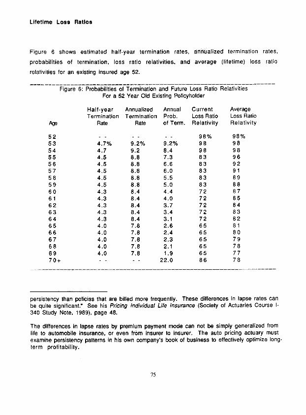
Figure 6 shows estimated half-year termination rates, annualized termination rates,
probabilities of termination, loss ratio relativities, and average (lifetime) loss ratio
relativities for an existing insured age 52.
----------______________________________~~~~~~~~~~~--------- _----- Figure 6: Probabilities of Termination and Future Loss Ratio Relativities
pge 52 _ _ 53 4.7% 54 4.7 55 4.5 56 4.5 57 4.5 58 4.5 59 4.5 60 4.3 61 4.3 62 4.3 63 4.3 64 4.3 65 4.0 66 4.0 67 4.0 68 4.0 69 4.0 70+ _ _
For a 52 Year Old Existing Policyholder
Half-year Annualized Annual Current Average Termination Termination Prob. Loss Ratio Loss Ratio
Rate Rate of Term. Relativity Relativity
_ _ 9.2% 9.2 8.8 8.8 8.8 8.8 8.8 8.4 8.4 8.4 8.4 8.4 7.8 7.8 7.8 7.8 7.8
_ _ 98% 98% 9.2% 98 98 8.4 98 98 7.3 83 96 6.6 83 92 6.0 83 91 5.5 83 89 5.0 83 88 4.4 72 87 4.0 72 85 3.7 72 84 3.4 72 83 3.1 72 82 2.6 65 81 2.4 65 80 2.3 65 79 2.1 65 78 1.9 65 77
22.0 86 78
persistency than policiss that are billed more frequently. These differences in lapse rates can be quite significant.” See his Pricing lncfividual Life insurance (Society of Actuaries Course l- 340 Study Note, 1989), page 48.
The differences in lapse rates by premium payment mode can not be simply generalized from life to automobile insurance, or even from insurer to insurer. The auto pricing actuary must examine persistency patterns in his own company’s book of business to effectively optimize long. term profitability.
75
At age 70 and up, termination rates do not vary significantly by age of the insured. To simplify
the calculations, we assume that the average insured who turns age 70 will keep his policy for
another 5 years, and his expected loss ratio relativity will be 0.86 (see Figure 1).
The numbers shown in Figure 6 are easily derived: we illustrate with the probability that a 52
year old insured will terminate at age 56. The probabilities that he will terminate at ages 53,
54, and 55 are 9.2%, 8.4%, and 7.3%, respectively. Thus, the probability that this insured
will renew into his 56th year is 1 .OOO - 0.092 - 0.084 - 0.073, or 76.1%.
His expected half-year termination rate at age 56 is 4.5%, which annualizes to 8.8%. The
probability that he will terminate at age 56 is therefore 8.8% l 76.1%, or 6.7%.
If he terminates at age 56, his expected loss ratio relativities are two and a half years of 98%
and one and a half years of 83%, for an average of 92%. (We are using the quinquennial loss
ratio relativities of Figure 2.) Note that policy terminations are assumed to occur on
anniversaries, whereas loss ratio relativities span the duration of the policy. In other words,
the average insured age 52 is actually 52 and a half, and his policy anniversary occurs when he
is 56 and a half.28
Life actuaries use similar (“asset share”) models.29 Since life policies pay a fixed dollar
benefit on death or maturity, the actuary must discount future payments for interest.
Automobile insurance claims vary with inflation, and premium rates are reset each year by the
insurer. The fixed dollar profits of the insurer increase with inflation, but their present
values remain the same. Therefore, discounting the future loss ratio relativities is incorrect.30
28 Since the loss ratio relativities used here are crude estimates, this precision is not necessary. If the actuary does have good persistency and loss ratio relativity figures, however, accurate predictions of profits are worthwhile.
2s See, for instance, David B. Atkinson, Gross Premiums and Asset Shares, Society of Actuaries Part 7 Study Note (19871, or David B. Atkinson, Pricing Individual Life Insurance, Society of Actuaries Course l-340 Study Note (1989).
so In truth, a slight discount is needed, since the insurer’s discount rate is normally higher than either the inflation rate or the loss cost trend rate. The inflation rate adjusts the nominal value of money to real terms. The insurer’s discount rate incorporates other factors as
76
We weight the average lifetime loss ratio relativities, given termination at a specific age, by the
probabilities of termination at each age. The expected future loss ratio relativity for the 52
year old existing insured is 87%. In other words, even with a 10% discount for the 52 year old
insured, the insurer will realize greater profits than on its overall book of business.
But whai discount should the pricing actuary recommend? So far we have examined the
implications of persistency patterns for premium discounts. Now we must analyze the
influences of premium discounts on persistency and production.
Prices, Persistency, and Production
Why offer any discount to the 52 year old insured ? Clearly, if no discount is offered, existing
policyholders may switch to competing carriers, and production of new business may decline.
The larger the discount, the greater the probability that existing insureds will renew their
policies and that new risks will be attracted.
In other words, the size of the discount affects persistency patterns and new business production
well, such as management’s desires for immediate profits and the probability of adverse changes in the insurance marketplace. Although they can be important, these additional influences on the discount rate are hard to quantify, so we have ignored them in the calculations.
Note the difference between the discount rate discussed here and that used to determine the present value of future loss payments. Future loss payments are negative cash flows, so many actuaries recommend using either a risk free rate or a downward “risk-adjusted” rate. See, for example, Richard G. Wolf, “Insurance Profits: Keeping Score,” in Financial Analysis of insurance Companies (Casualty Actuarial Society 1987 Discussion Paper Program), pages 446-533, and Robert P. Butsic, “Determining the Proper Interest Rate for Loss Reserve Discounting: An Economic Approach,” in Evaluating insurance Company Liabiliries (Casualty Actuarial Society 1988 Discussion Paper Program) pages 147-188. For the analysis of this paper, we are examining future profits. If the future profits were expressed in dollars, instead of loss ratios, we would use a cost of capital rate to determine the present values. See, for example, the estimate of the National Council on Compensation Insurance for its Internal Rate of Return pricing model in NCCI Actuarial Operations Memorandum AC-47 (July 25, 1989), Exhibit 27-1. The difference between the NCCl’s cost of capital rate (16% in 1989) and Butsic’s risk adjusted loss resew8 discount rate (4% in 1987) is enormous. This is due to the different purposes of these discount rates, not to any controversy over method.
rates. Given such patterns and rates, we can estimate the expected long-term profits for the
insurer. The optimal discount is the one that maximizes the long-term profits.31 Thus, the
optimal discount is between 0% and 13% - depending on the effect of the discount on
persistency patterns for existing policyholders and production rates for new policyholders.32
We have come full circle. Price elasticity of demand - or persistency patterns and new
business production rates - influences the optimal premium discount. Conversely, the
premium discount influences the persistency patterns and new business production rates.
Persistency patterns for older insureds are not much affected by small rate discounts. New
business production, however, does depend on price levels. Most importantly, an insurer’s
market share for retired drivers is significantly in!luenced by its rate discounts for these
drivers in prior years - before retirement.
Two items complicate the analysis now. First, actuaries examine historical experience to
forecast the future. Since conditions change frequently, we desire to use current data - the most
recent year or two of experience. But the effects of premium discounts on long-term
persistency patterns are not evident for years. Clearly, we can not wait a decade before deciding
what price to charge.
Second, many factors affect persistency patterns and new business production rates. Premium
discounts are one factor. Other considerations include marketing efforts, underwriting
31 Note how different the traditional actuarial philosophy is, which sees the appropriate discount as the one indicated by the experience. But even a “warranted” discount reduces profits if it has no effect on persistency or production.
Our traditional pricing techniques seek rate equity among insureds. But rate equity rarely optimizes net income. The actuary must consider the degree of competition by line of business, classification, and territory, the price elasticity of demand along the same dimensions, and the rate structures of peer companies when devising an optimal pricing system. These issues are complex, and will be treated at length in a separate paper. The goal of this article is simply to show the effect of persistency patterns on pricing procedures. In practice, the remaining factors, such as competition and peer company prices, must be considered as well.
32 Since new insureds have higher termination rates, the upper bound for the discount is actually below 13%. In practice, one should examine long-term profits by the insured’s age at policy issue. We have avoided this in the text, simply to keep the mathematics simple.
78
philosophy, competitive levels, peer company rates, and state regulation. The experience may
be so cloudy that the underlying patterns are obscured.
This only means that the task is more challenging, not that it should be avoided. But how should
the pricing actuary approach this problem?
The most straightforward method is to collect data on changes in persistency patterns and new
business production rates resulting from revisions in other rate relativities. For instance,
suppose an insurer increases the discount on the second automobile in a multi-car risk from
20% to 30%. If it keeps information about persistency patterns and new business production
both before and after the change, it will be better able to estimate the effects of rate relativity
revisions.
Unfortunately, persistency patterns vary greatly by classification. A premium discount may
influence the middle-aged driver’s decision to renew, but a discount of the same magnitude may
have less effect on the renewal decision of a retired driver. Similarly, discounts have differing
effects on production among different market segments.
Inverse Analyses
An alternative, but not necessarily a better one, is to use inverse analyses. We may be able to
predict the effects of a new program by examining the experience before the program was
instituted. Specifically, if other large insurers have instituted a similar older driver discount
at an earlier time, we may be able to discern the effects in our own company’s production and
persistency patterns. A hypothetical example should illustrate this: the data are heuristic only,
and do not correspond to actual experience.
Suppose your insurer began offering an automobile discount for refired drivers age 55 and
above in 1980. Your major competitor began offering discounts for a// drivers age 50 and
above at that time, not just for those who were retired. Furthermore, suppose that the new
business exposure distributions for automobile insurance by age of the principal operator for
your company between 1981 and 1987 are as shown in Figure 7.
79
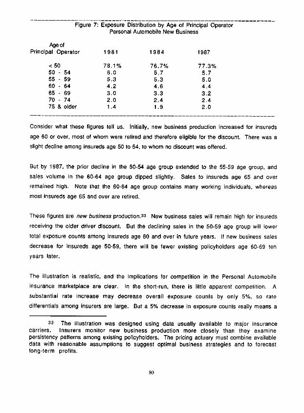
-----___-----___-------------------------------------------------- Figure 7: Exposure Distribution by Age of Principal Operator
Personal Automobile New Business
Age of Principal Operator 1981 1984 1987
< 50 78.1% 76.7% 77.3% 50 - 54 6.0 5.7 5.7 55 - 59 5.3 5.3 5.0 60 - 64 4.2 4.6 4.4 65 - 69 3.0 3.3 3.2 70 - 74 2.0 2.4 2.4 75 8 older 1.4 1.9 2.0
----___-_--_____________________________--------------------------
Consider what these figures tell us. Initially, new business production increased for insureds
age 60 or over, most of whom were retired and therefore eligible for the discount. There was a
slight decline among insureds age 50 to 54, to whom no discount was offered.
But by 1987, the prior decline in the 50-54 age group extended to the 55-59 age group, and
sales volume in the 60-64 age group dipped slightly. Sales to insureds age 65 and over
remained high. Note that the 60-64 age group contains many working individuals, whereas
most insureds age 65 and over are retired.
These figures are new business production.33 New business sales will remain high for insureds
receiving the older driver discount. But the declining sales in the 50-59 age group will lower
total exposure counts among insureds age 60 and over in future years. If new business sales
decrease for insureds age 50-59, there will be fewer existing policyholders age 60-69 ten
years later.
The illustration is realistic, and the implications for competition in the Personal Automobile
insurance marketplace are clear. In the short-run, there is little apparent competition. A
substantial rate increase may decrease overall exposure counts by only 5%, so rate
differentials among insurers are large. But a 5% decrease in exposure counts really means a
3s The illustration was designed using data usually available to major insurance carriers. Insurers monitor new business production more closely than they examine persistency patterns among existing policyholders. The pricing actuary must combine available data with reasonable assumptions to suggest optimal business strategies and to forecast long-term profits.
80
5% decrease in exposures for the next ten years, even if rates are subsequently lowered. The
effects of price on profitability may be subtle, but in the long-run, they are powerful.34
Unfortunately, inverse analyses are sometimes of little help. Generally, the pricing actuary
must forecast the probable effects of a new program before competitors have instituted it.
Waiting ten years to quantify the damage caused by delay is not a sound business strategy either.
The recommendation in a previous footnote is worth repeating: you must combine the available
data with reasonable assumptions to forecast future income.
Cross Product Effects
Large Commercial Lines insurers do not market their products in isolation. A carrier may offer
Commercial Automobile coverage at a substantial discount in hopes of securing the more
profitable Workers’ Compensation or General Liability business.35 Similar marketing
philosophies benefit the Personal Lines insurer as well.
Consumers purchase various insurance coverages, such as automobile, homeowners’, life, and
health insurance. Many individuals have several policies with the same insurer, for at least
two reasons.
34 The same phenomenon is apparent in the rise of the direct writers in the Personal Lines marketplace. Direct writers must sink large expenses in creating or expanding an agency system, and they pay high first year commissions. Net income during the first few years rarely compensates for these expenses.
Twenty years later, however, the situation has changed dramatically. Renewal commissions are low, and Personal Lines policyholder loyalty is high. Total distribution expenses are much lower than those which independent agency companies incur. Both net income and market share grow steadily. In other words, even powerful effects of operating changes may be hidden for long periods. See Paul L. Joskow, “Cartels, Competition, and Regulation in the Property-Liability Insurance Industry,” The Bell Journal of Economics and Management Science, Volume 4, Number 2 (Autumn t987), pages 375-427, for further comments on expense ratios and entry barriers for direct writers.
3s In underwriting parlance, the Commercial Automobile coverage is a “loss leader” in “account pricing.”
81
First, the insurance agent may recommend an additional coverage to an existing policyholder.
Similarly, the consumer may like a particular agent, and switch his existing coverages to that
agent’s insurer.
Second, much advertising has little effect on the public. Consumers are inundated with magazine
ads and television commercials, and they ignore most of what they see or hear. But consumers
are receptive to information from or about firms with which they deal. An advertisement for
Homeowners’ insurance makes a strong impression upon that carrier’s current automobile
insureds.
Thus, an automobile insurance premium discount for policyholders nearing retirement may
bring additional Homeowners’ sales in addition to the automobile business. But will this
business be profitable?
Consider again Figure 1. By the time a driver reaches his 75th year, he is rarely a good risk.
Physical deterioration progresses, and accident frequencies increase. Those individuals aware
of their limited abilities often cease driving and terminate their policies. In either case, profits
for the insurer soon end.
Homeowners’ hazards are related to the insured’s activities. A family with children, pets,
adolescents, and numerous friends is exposed to all sorts of perils: fire, vandalism, liability,
glass, and water damage. As the children mature and leave home, and as pets and rowdy friends
disperse, the hazards decrease. Yet the home remains, so the homeowner retains the insurance
coverage. Figure 7 shows Homeowners’ loss ratios for older insureds.
82
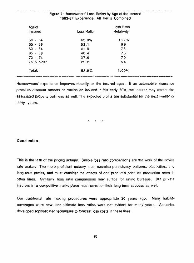
Age of insured
50 - 54 6 3 . 0 % 117% 55 - 59 53.1 99 60 - 64 41.8 78 65 - 69 40.4 75 70 - 74 37.6 70 75 8. older 29.2 54
Total:
Figure 7: Homeowners’ Loss Ratios by Age of the Insured 1983-87 Experience, All Perils Combined
Loss Ratio Loss Ratio Relativity
53.9% 1 .OO%
Homeowners’ experience improves steadily as the insured ages. If an automobile insurance
premium discount attracts or retains an insured in his early 50’s, the insurer may attract the
associated property business as well. The expected profits are substantial for the next twenty or
thirty years.
l t .
Conclusion
This is the task of the pricing actuary. Simple loss ratio comparisons are the work of the novice
rate maker. The more proficient actuary must examine persistency patterns, elasticities, and
long-term profits, and must consider the effects of one product’s price on production rates in
other lines. Similarly, loss ratio comparisons may suffice for rating bureaus. But private
insurers in a competitive marketplace must consider their long-term success as well.
Our traditional rate making procedures were appropriate 20 years ago. Many liability
coverages were new, and ultimate loss ratios were not evident for many years. Actuaries
developed sophisticated techniques to forecast loss costs in these lines.
83

Different forecasts are now demanded of us. Our employers no longer ask us merely to estimate
future losses. Now they want to know: “What competitive strategy is best for us? What market
segments should we target? How might our pricing philosophy help us attain the future we
envision?” These are harder problems to solve, since the data are fuzzy and the conclusions are
slippery. So the challenge we face is all the greater.
84