Perspectives of New Music is collaborating with JSTOR to ...sites.music.columbia.edu/cmc/courses/g6611/spring2012/week12/Gendy3.pdfXenakis proposes starting with an aperiodic sound

Stochastic Composition and Stochastic Timbre: GENDY3 by Iannis XenakisAuthor(s): Marie-Hélène SerraReviewed work(s):Source: Perspectives of New Music, Vol. 31, No. 1 (Winter, 1993), pp. 236-257Published by: Perspectives of New MusicStable URL: http://www.jstor.org/stable/833052 .Accessed: 02/04/2012 16:53

Your use of the JSTOR archive indicates your acceptance of the Terms & Conditions of Use, available at .http://www.jstor.org/page/info/about/policies/terms.jsp

JSTOR is a not-for-profit service that helps scholars, researchers, and students discover, use, and build upon a wide range ofcontent in a trusted digital archive. We use information technology and tools to increase productivity and facilitate new formsof scholarship. For more information about JSTOR, please contact [email protected].

Perspectives of New Music is collaborating with JSTOR to digitize, preserve and extend access to Perspectivesof New Music.

http://www.jstor.org

http://www.jstor.org/action/showPublisher?publisherCode=pnm

http://www.jstor.org/stable/833052?origin=JSTOR-pdf

http://www.jstor.org/page/info/about/policies/terms.jsp

STOCHASTIC COMPOSITION AND STOCHASTIC TIMBRE:

GENDT3 BY IANNIS XENAKIS

MARIE-HELENE SERRA

ABSTRACT

GENDY3 BY IANNIS XENAKIS is a stochastic music work entirely pro- duced by a computer program written in 1991 by the composer him-

self at CEMAMu. The work GENDT3 is the continuation of the series of stochastic music works that Xenakis inaugurated in 1955 with Metastasis. In GENDT3, the use of stochastic rules is more deeply systematic, as the composer says in his recent publication (Xenakis 1991b). Not only is the musical structure of GENDT3 stochastic, but the sound synthesis is also based on a stochastic algorithm that Xenakis invented and called "dynamic stochastic synthesis." In this paper, we describe the whole process of the computation of GENDT3, from the low-level sound produc- tion to the high-level global architecture. We also take up aspects which

GENDY3 by lannis Xenakis 237

GENDY3 has in common with earlier stochastic works which Xenakis composed and described in Formalized Music (Xenakis 1971).1 The stochastic program that was used for the composition of GENDT3 is partly listed in the new edition of Formalized Music (Xenakis 1991a).

INTRODUCTION

Stochastic music emerged in the years 1953-55, when Iannis Xenakis introduced the theory of probability in music composition. First, probability calculus was used in Metastasis,2 then in Pithoprakta,3 for the generation of a great number of "speeds," which are represented as lines in the pitch-time space (Xenakis 1971). Then Xenakis decided to generalize the use of probabilities in music composition. The work Achorripsis4 was his first work towards this generalization. In Achorripsis, a small number of stochastic rules are applied to generate both the parameters of the notes and the global structure. The architecture of the piece can be read in a two-dimensional matrix that is defined in a space where seven rows representing seven groups of instruments evolve in time (see Example 1). The matrix represents the global distribution of the sound matter; only one parameter, the sound density, obeys a Poisson law in this two- dimensional space. The lower levels are also organized with stochastic functions; for instance, the durations and the pitches of the notes. At that time all the stochastic computations were made by hand or with the help of calculating machines that were rudimentary.

In the 1960s, Xenakis started to use the computer to automate and accelerate the many stochastic operations that were needed, entrusting the computer with important compositional decisions that are usually left to the composer. For example, in the work ST10,5 the composition of the orchestra (expressed in percentages of groups of instruments) is computed by the machine, as well as the assignment of a given note to an instrument of the orchestra. At the end of the computation of the musical work, the numerical results were transcribed into traditional notation so that the music could be played by an orchestra. At this time, speaking about the ST program, Xenakis declared: "Although this program gives a satisfactory solution to the minimal structure, it is, however, necessary to jump to the stage of pure composition by coupling a digital-to-analog converter to the computer"6 (Xenakis 1971).

In the 1960s, Xenakis put forward the idea of extending the use of stochastic laws to all the levels of the composition, including sound produc- tion. This proposition was renewed in 1971:

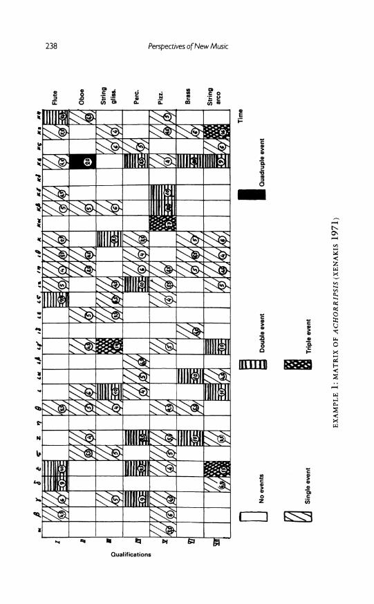
No events

X Single event

; Double event I Quadruple event

Triple event

EXAMPLE 1: MATRIX OF ACHORRIPSIS (XENAKIS 1971)

0 c

al

_. o

hu Flute

Oboe

String gliss.

Perc.

Pizz.

Brass

String arco

o

C(

0

z CD

Time

GENDY3 by lannis Xenakis

Any theory or solution given on one level can be assigned to the solution of problems of another level. Thus the solutions in macro- composition (programmed stochastic mechanisms) can engender simpler and more powerful new perspectives in the shaping of microsounds than the usual trigonometric functions can . . . All music is thus homogenized and unified.7(Xenakis 1971)

In the 1970s, at the University of Indiana, Xenakis experimented with new methods for synthesizing sounds based on random walks (Xenakis 1971),8 the theoretical aspects of which are described in probability theory (Feller 1968).

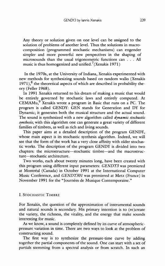
In 1991 Xenakis returned to his dream of making a music that would be entirely governed by stochastic laws and entirely computed. At CEMAMu,9 Xenakis wrote a program in Basic that runs on a PC. The program is called GENDY: GEN stands for Generation and DY for Dynamic; it generates both the musical structure and the actual sound. The sound is synthesized with a new algorithm called dynamic stochastic synthesis, with this algorithm one can generate a great variety of different families of timbres, as well as rich and living sounds.

This paper aims at a detailed description of the program GENDY, whose main aspect is its stochastic synthesis algorithm. Indeed, we will see that the form of the work has a very close affinity with older stochastic works. The description of the program GENDY is divided into two chapters: the microstructure-stochastic timbre-and the macrostructure-stochastic architecture.

Two works, each about twenty minutes long, have been created with this program using different input parameters: GENDT3 was premiered at Montreal (Canada) in October 1991 at the International Computer Music Conference, and GENDT301 was premiered at Metz (France) in November 1991 for the "Journees de Musique Contemporaine."

I. STOCHASTIC TIMBRE

For Xenakis, the question of the approximation of instrumental sounds and natural sounds is secondary. His primary intention is to (re)create the variety, the richness, the vitality, and the energy that make sounds interesting for music.

As we know, a sound is completely defined by its curve of atmospheric- pressure variation in time. There are two ways to look at the problem of constructing sound.

The first way is to synthesize the pressure-time curve by adding together the partial components of the sound. One can start with a set of partials stemming from a spectral analysis or from scratch. In such an

239

Perspectives of New Music

approach, the complexity of the sound is built by piling up and, if neces-

sary, varying the individual sound components until the desired sound is reached. For instance, one can start with a group of sine harmonics and progressively inject aperiodicity into the sound by varying the frequency and the amplitude of the harmonics.

For Xenakis this approach, based on Fourier analysis, is not adequate for (re)synthesizing the complexity inherent in sound. He prefers to take a global approach in which the sound synthesis is performed only in the time domain, without resorting to spectral decomposition. Instead of

starting with a periodic sound and modifying it (including random variations), he starts ". .. from a disorder concept and then introduce(s) means that would increase or reduce it" (Xenakis 1985). In other words, Xenakis proposes starting with an aperiodic sound (a random signal) into which different degrees of regularity are injected.

In the early 1970s, at the Center for Mathematical and Automated Music (CMAM) at Indiana University, Xenakis experimented with vari- ous types of random walks for synthesizing sound (Xenakis 1971). The idea was to assign a given particle's position to the amplitude of each sample of the sound, which particle moved in an aleatory fashion on one axis; barriers (elastic or absorbing) were added for controlling the particle's random positions. As will be shown, the concept of random walks, i.e. random motions and barriers, is also found in dynamic stochastic synthesis.

1.1 THE PROGRAM GENDY

The program GENDY computes a series of numerical samples and stores them in a sound file that can be played after the computation is over. The amplitude of one sample is the sum of the amplitudes given by several voices. A voice is characterized by a set of input parameters, including the stochastic synthesis parameters that control the sound. There are up to sixteen voices. Two sound files may be played at the same time, so that the number of voices can be increased and stereo effects can be integrated into the music.

1.2 THE SYNTHESIS MODEL

Many sounds, especially sounds coming from many musical instruments, may be viewed in a general way as a succession of waveforms which are repeated in time with more or less variation. For example, many instrumental sounds can be schematized in three parts: attack, sustain, and release. The sustain is a relatively stable part, often quasi-

240


periodic; it can be described as the repetition of a typical shape (the period) which is modified, mainly in amplitude but also slightly in frequency. In the attack part, there is no or very little periodicity. The attack can be modelled as a waveform whose modification from one repetition to another is very large.

In the dynamic stochastic synthesis model, it is assumed that the sound is made of the repetition of an initial waveform and that at each repetition the shape of the waveform is distorted according to both time and amplitude. The synthesis algorithm consists in computing each new waveform by applying stochastic variations to the previous one.

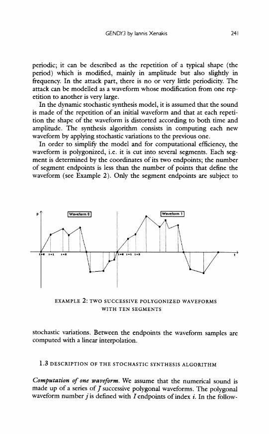
In order to simplify the model and for computational efficiency, the waveform is polygonized, i.e. it is cut into several segments. Each segment is determined by the coordinates of its two endpoints; the number of segment endpoints is less than the number of points that define the waveform (see Example 2). Only the segment endpoints are subject to

P [Waveform 01 Waveform 1

i- i-1 i-2 i -1 ti-2

EXAMPLE 2: TWO SUCCESSIVE POLYGONIZED WAVEFORMS WITH TEN SEGMENTS

stochastic variations. Between the endpoints the waveform samples are computed with a linear interpolation.

1.3 DESCRIPTION OF THE STOCHASTIC SYNTHESIS ALGORITHM

Computation of one waveform. We assume that the numerical sound is made up of a series of J successive polygonal waveforms. The polygonal waveform number j is defined with I endpoints of index i. In the follow-

241


ing, we note the coordinates of the endpoints (see Example 2) as

(xi, Yi, j), 0 < i< I, 0 <j<J.

The abscissae x. , are sample numbers.11 The ordinates i j are 16-bit

integers.12 Continuity between two successive waveforms is guaranteed by stipulating that the endpoint number 0 (first endpoint) in waveform

j+ 1 is equal to the endpoint number I- 1 (last endpoint) in waveform

.:

(Xo, j+ , ,j+) = (XI- 1, I-I ,j) (1)

At this time, the number of endpoints Iin the waveform is supposed to be constant. Therefore, for any j, the number of endpoints in waveform

j+ 1 is the same as in waveform j. The coordinates of each endpoint in waveform j+ 1 are obtained by adding a stochastic variation to the coordinates of the corresponding endpoint (endpoint of same rank) in waveform j. We note this process by the set of expressions (2):

xi,j+ = xij+fx() (2.1)

Yi,j+ = Yi,j+fy(z) (2.2)

where fx(z) and fy(z) are the values (positive or negative) returned by the stochastic functions fx and fy, for the argument z, which is itself a random number with uniform distribution.

The duration di, in seconds of the segment lying between the two

endpoints i and i+1 is proportional to the number of samples ni,j in the

segment:

di = (nij- 1)/Srate(sec)

ni,j Xi+1,j+1 -

ij+1 +

where Srate is the sampling rate, in our case 44100 samples per second. The total duration D of the waveform is equal to the sum of the seg- mental durations:

I-1

D = E di (3) i=0

242


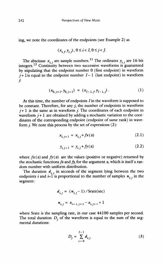
If the abscissae xi were not subjected to any variation, we would get only a nonlinear amplitude variation of the waveform over time.13 Since both the abscissae xi j and the ordinates yi . of the segment endpoints vary, the polygonal waveform varies both in shape and in duration, lead-

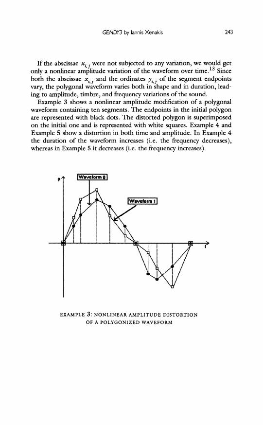
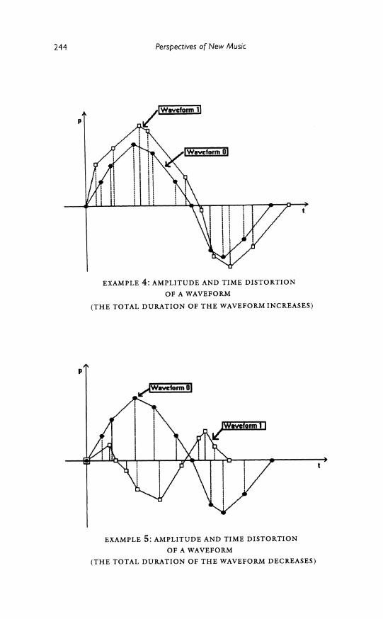
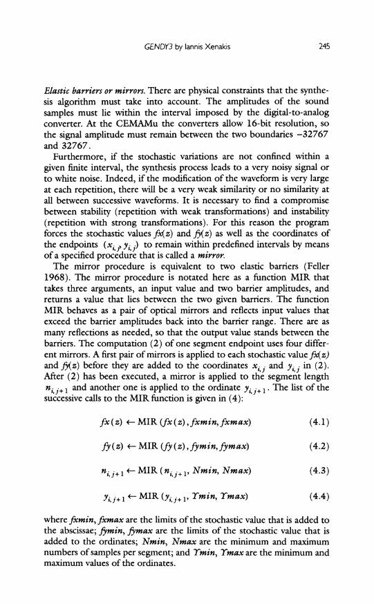
ing to amplitude, timbre, and frequency variations of the sound. Example 3 shows a nonlinear amplitude modification of a polygonal

waveform containing ten segments. The endpoints in the initial polygon are represented with black dots. The distorted polygon is superimposed on the initial one and is represented with white squares. Example 4 and

Example 5 show a distortion in both time and amplitude. In Example 4 the duration of the waveform increases (i.e. the frequency decreases), whereas in Example 5 it decreases (i.e. the frequency increases).

EXAMPLE 3: NONLINEAR AMPLITUDE DISTORTION

OF A POLYGONIZED WAVEFORM

243


p

EXAMPLE 4: AMPLITUDE AND TIME DISTORTION

OF A WAVEFORM

(THE TOTAL DURATION OF THE WAVEFORM INCREASES)

p

t

EXAMPLE 5: AMPLITUDE AND TIME DISTORTION

OF A WAVEFORM

(THE TOTAL DURATION OF THE WAVEFORM DECREASES)

244


Elastic barriers or mirrors. There are physical constraints that the synthesis algorithm must take into account. The amplitudes of the sound

samples must lie within the interval imposed by the digital-to-analog converter. At the CEMAMu the converters allow 16-bit resolution, so the signal amplitude must remain between the two boundaries -32767 and 32767.

Furthermore, if the stochastic variations are not confined within a

given finite interval, the synthesis process leads to a very noisy signal or to white noise. Indeed, if the modification of the waveform is very large at each repetition, there will be a very weak similarity or no similarity at all between successive waveforms. It is necessary to find a compromise between stability (repetition with weak transformations) and instability (repetition with strong transformations). For this reason the program forces the stochastic values fx(z) and f(z) as well as the coordinates of the endpoints (xi, Yi j) to remain within predefined intervals by means of a specified procedure that is called a mirror.

The mirror procedure is equivalent to two elastic barriers (Feller 1968). The mirror procedure is notated here as a function MIR that takes three arguments, an input value and two barrier amplitudes, and returns a value that lies between the two given barriers. The function MIR behaves as a pair of optical mirrors and reflects input values that exceed the barrier amplitudes back into the barrier range. There are as many reflections as needed, so that the output value stands between the barriers. The computation (2) of one segment endpoint uses four different mirrors. A first pair of mirrors is applied to each stochastic value fx(z) and fy(z) before they are added to the coordinates xij and i j in (2). After (2) has been executed, a mirror is applied to the segment length n, j+ 1 and another one is applied to the ordinate Yi, j+ The list of the successive calls to the MIR function is given in (4):

fx(z) - MIR (fx(z), fxmin, fxmax) (4.1)

fy(z) - MIR (fy(z), fymin, fymax) (4.2)

ni j+ 1 <- MIR (nij+ 1, Nmin, Nmax) (4.3)

Yi, j+ 1 - MIR (Yi, j+ 1, min, Ymax) (4.4)

where fxmin, fxmax are the limits of the stochastic value that is added to the abscissae; fimin, fimax are the limits of the stochastic value that is added to the ordinates; Nmin, Nmax are the minimum and maximum numbers of samples per segment; and Ymin, Ymax are the minimum and maximum values of the ordinates.

245


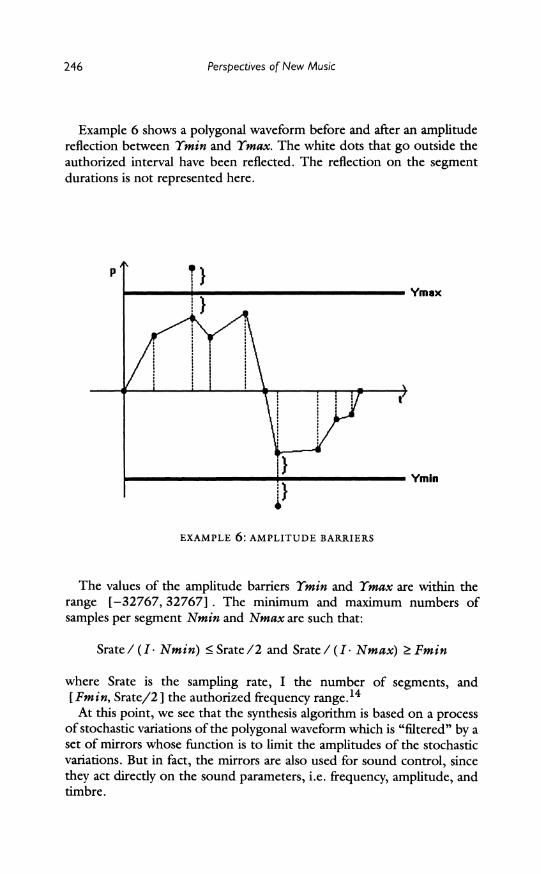
Example 6 shows a polygonal waveform before and after an amplitude reflection between Ymin and Ymax. The white dots that go outside the authorized interval have been reflected. The reflection on the segment durations is not represented here.

p

Ymax

EXAMPL 6:APIUEYmIn ,,-- -- Ymin

EXAMPLE 6: AMPLITUDE BARRIERS

The values of the amplitude barriers Ymin and Ymax are within the range [-32767, 32767]. The minimum and maximum numbers of samples per segment Nmin and Nmax are such that:

Srate / ( I Nmin) < Srate/2 and Srate / ( I Nmax) > Fmin

where Srate is the sampling rate, I the number of segments, and [Fmin, Srate/2] the authorized frequency range.14

At this point, we see that the synthesis algorithm is based on a process of stochastic variations of the polygonal waveform which is "filtered" by a set of mirrors whose function is to limit the amplitudes of the stochastic variations. But in fact, the mirrors are also used for sound control, since they act directly on the sound parameters, i.e. frequency, amplitude, and timbre.

246


For instance, the sound fundamental frequency, which is inversely proportional to the waveform duration Dj(3), depends on the total number of segments I, and on the two pairs of barriers, (fxmin, fxmax) and (Nmin, Nmax). A sound with a slightly varying pitch can be obtained by imposing a small variation interval (fxmin, fxmax) in conjunction with a reduced range (Nmin, Nmax). Nmin and Nmax are such that the interval (Srate/I. Nmax), (Srate/I- Nmin) contains the desired average frequency.15 In the same way, by increasing or decreasing the amplitudes of the barriers (Ymin, Ymax), we can control the amount of reflections which in turn control the signal's shape, and which naturally relates to the timbre.

At this time we do not know exactly how to formalize and quantize the effect of the mirrors on the sound parameters. The mathematical aspect of the stochastic synthesis algorithm is at this time under study.

1.4 THE INPUT PARAMETERS OF STOCHASTIC DYNAMIC SYNTHESIS

The input parameters of the sound synthesis model may be separated into two groups:

(a) the number of segments in the waveform I the stochastic distributionfx the mirror boundaries (fxmin, fxmax), (Nmin, Nmax) (b) the stochastic distribution f the mirror boundaries (fymin, fymax), ( min, Ymax)

The first group primarily controls the pitch whereas the second group controls the sound amplitude and timbre.

This set of parameters is preestablished by the user for each voice in each section (see section II) and is constant over time. The experiments consist of varying the different input parameters so that we can identify different classes of effects on the sound results.

In the next section we list the different types of stochastic distributions that Xenakis uses in his program, and explain the details of the computation of the stochastic values fx(z) and fy(z).

1.5 STOCHASTIC DISTRIBUTIONS

We see from (2) that the program must generate two series of stochastic values that we expressed as fx(z) and fy(z) and that follow the given stochastic functions fx and fy. In order to clarify what the program does at this step of the computation, we first mention some fundamental results of the theory of probability (Feller 1968).

247


Sample space Q and random variable x. We can speak of probabilities in relation to a given sample space. The sample space fl is the set of all the elementary events of the experiment that we consider. For instance, in the coin-tossing game, the sample space Qf is made of two elementary events, "head" and "tail." Each elementary event in the sample space has its probability of occurrence. In the coin-tossing game the probability of heads is 1/2. The probability of combined events (events formed of unions, intersections of elementary events) may be computed from the probabilities of elementary events.

A random variable is a numerical function that associates numerical values to the events of Qf. A random variable is either continuous or discrete. It is discrete if it takes only a finite or countable set of values. It is continuous if it can take all real values in a given interval (or several intervals). For instance, in the coin-tossing game we can build a discrete random variable X that takes the value 1 if the event "head" is realized and the value minus 1 if the event "tail" is realized.

The expression X = x designates the set of events in Q that are associ- ated to the value x by the function X. Similarly the expression X <= x designates the set of events in Q that take values ranging from -oo to x. A random variable is real if its values belong to the set of real numbers R. In the following we will consider continuous and real random variables.

Distribution function of x and probability density of X. A continuous random variable is defined by the values it takes (often a mathematical function) and also by the probabilities of getting those values, which are related to the probabilities of the events in math.

The function that describes the probabilities of the values ofXis called the distribution function F(x). The distribution function F is defined by F (x) = P [ X x] , where P [ X< x] is the probability that the random variable X takes values ranging from -oo to x.

If the distribution function F is differentiable, the random variable X admits a densityfunction f such that

x

F(x) = ff(t)dt.

Examples of densityfunctions. In this section we list several density functions f (x) and their corresponding distribution functions F(x) that are used in the GENDY composition program (Feller 1968; Xenakis 1971).

The uniform distribution on an interval [0, A]:

248


forx<Of(x) = 0 F(x) =0

for O0<x<A f(x) = 1/A F (x) = x/A

for x>A f(x) = O F (x) = 1.

The Cauchy density centered at the origin is defined by:

1 t 1 1 for-oo<x<oo,f(x) = 1 2 ,F(x) = -+

t+ x 2 Ttan-1 (x/t)

The logistic density: -ax- b f O ff ) -ae F () 1

for a > 0, -0o <x< oo,f() = , F(x) = - -ax- b 2 +

-ax-b (1+ l+e

The exponential density:

2 a2x -a2x for x 0,f(x) = ae- x,F(x) = l--a2

for x< O,f(x) =0, F (x) =0.

Simulation of a random variable. In the program we have to build a series of stochastic values X with a corresponding distribution F. This means that we have to generate a series of numbers X such that the probability that X < x is an approximation of a given distribution function F(x). For that purpose we use the following theorem (Bestougeff 1975): if Y is a random variable with a uniform distribution on [0,1] and if the function F is invertible, then the random variable X that follows the distribution function F is obtained with:

x= F-1 (Y) (5)

where F-1 is the inverse ofF.

For instance, the random variable X that follows the exponential distribution is computed with:

X= -l/a -log(l - T).

249

(6)


From (4) we see that once we have a random variable Ywith a uniform distribution between [0,1], the computation of X is straightforward. In the program, we use the random generator in order to get a uniform random number that we called z in expression (2). Then we compute fx(z) and fy(z), where fx and fy represent the inverse functions of the desired stochastic distribution.

1.6 RESULTS

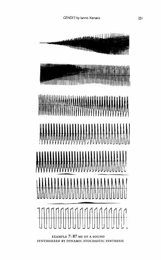
Very different families of timbres have been obtained with the dynamic stochastic algorithm. The sounds are usually very rich in harmonics and present a lively and dynamic quality that is noticeable. The polygoniza- tion of the waveform introduces discontinuities into the numerical signal that produce high partials, some of which will be aliased by the digital- to-analog conversion. Digital filtering can be applied in order to attenu- ate the aliasing, but then the signal may lose some variability that is valu- able for the dynamic quality.

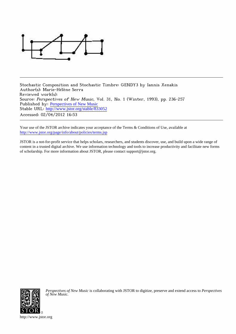
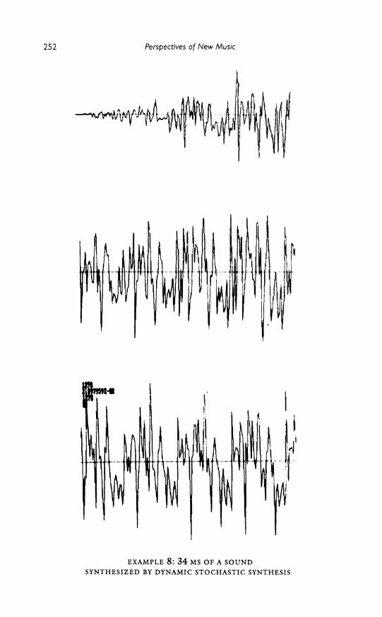
Examples 7 and 8 show two examples of sounds created with the dynamic stochastic algorithm. This method seems to be very attractive, and Xenakis is still working on it today. As we said, the number of segments in the waveform, the mirror boundaries, and the distribution functions are constant parameters for each voice in each section. Xenakis's research is now turned towards exploring the variation of these global parameters, in order to get global sound modifications over time.

II. STOCHASTIC ARCHITECTURE

In this section we describe the macrostructural level of the composition. The structure of GENDT3 can be considered in a two-dimensional space where time is the horizontal axis and where the vertical axis is used for the layout of different voices. This space is similar to the one used in Achorripsis (see Example 1) and in the ST pieces (Xenakis 1971), where the instrumental groups are distributed along the vertical axis (rows) and where the time axis is divided into sequences or sections (columns).

GENDT3 is a series of juxtaposed sections (time axis) in which we can find a different number of voices (vertical axis). On the time axis, the section itself is defined by a succession of time-intervals that are designated time-fields; the time-fields represent time portions where either silence or sound can be found; there is a different succession of time-fields for each voice. On the vertical axis, the section is defined by a voice-configuration. A voice-configuration is defined by the number of voices that play, the

250


)&1flVJ ,~t, tw

- -~~ - - - I,

EXAMPLE 7: 87 MS OF A SOUND SYNTHESIZED BY DYNAMIC STOCHASTIC SYNTHESIS

251


EXAMPLE 8: 34 MS OF A SOUND

SYNTHESIZED BY DYNAMIC STOCHASTIC SYNTHESIS

252


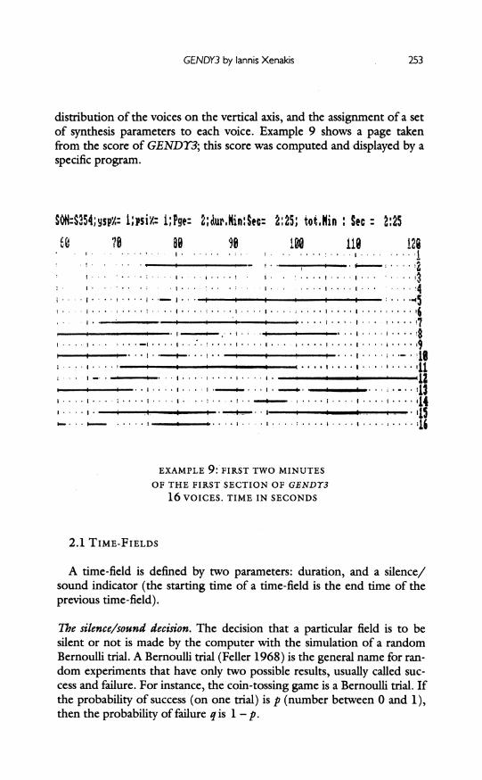
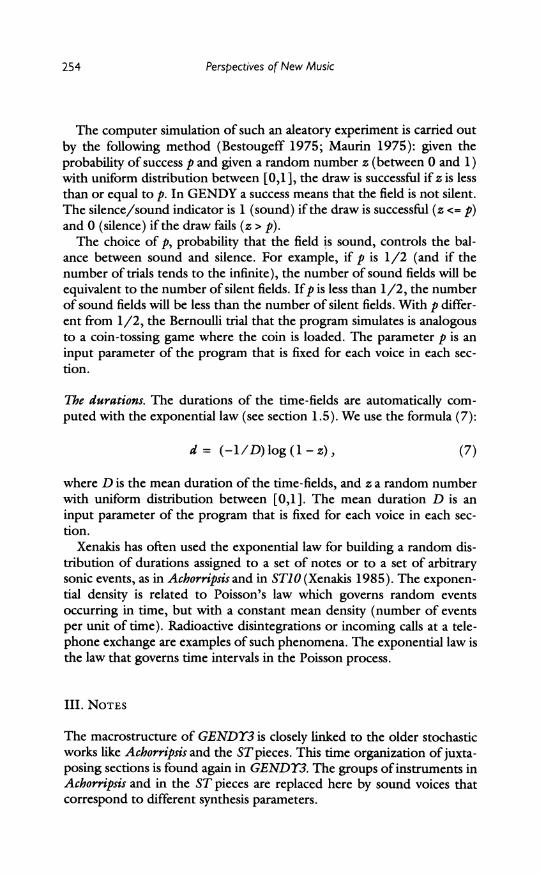
distribution of the voices on the vertical axis, and the assignment of a set of synthesis parameters to each voice. Example 9 shows a page taken from the score of GENDY3; this score was computed and displayed by a specific program.

SOHN:S54;ysp.=: i,si=: i;,Pe: 2;cur,.in:Set: 2:25; tot.Kin Sec 2:25 i , C 4 . I 6 78 80 5 t1B0 118 128

. ,*. . . , ; . . . . .;... |

. : a3 .... . .: , .... . . I .. .. , i ... .. ..I . ... ,4

. .... '

I .... .... ., ....... ... ..... ........ .... ,g. I .. .- i

EXAMPLE 9: FIRST TWO MINUTES

I .. OF THE FIRST SECTION OF GEND3'

16 VOICES. TIME IN SECONDS

2.1 TIME-FIELDS

A time-field is defined by two parameters: duration, and a silence/ sound indicator (the starting time of a time-field is the end time of the previous time-field).

The silence/sound decision. The decision that a particular field is to be silent or not is made by the computer with the simulation of a random Bernoulli trial. A Bernoulli trial (Feller 1968) is the general name for random experiments that have only two possible results, usually called success and failure. For instance, the coin-tossing game is a Bernoulli trial. If the probability of success (on one trial) is p (number between 0 and 1), then the probability of failure q is 1 - p.

253


The computer simulation of such an aleatory experiment is carried out

by the following method (Bestougeff 1975; Maurin 1975): given the probability of success p and given a random number z (between 0 and 1) with uniform distribution between [0,1], the draw is successful if z is less than or equal to p. In GENDY a success means that the field is not silent. The silence/sound indicator is 1 (sound) if the draw is successful (z <= p) and 0 (silence) if the draw fails (z > p).

The choice of p, probability that the field is sound, controls the bal- ance between sound and silence. For example, if p is 1/2 (and if the number of trials tends to the infinite), the number of sound fields will be equivalent to the number of silent fields. Ifp is less than 1/2, the number of sound fields will be less than the number of silent fields. With p different from 1/2, the Bernoulli trial that the program simulates is analogous to a coin-tossing game where the coin is loaded. The parameter p is an input parameter of the program that is fixed for each voice in each section.

The durations. The durations of the time-fields are automatically computed with the exponential law (see section 1.5). We use the formula (7):

d = (-1/D)log (1 - z), (7)

where D is the mean duration of the time-fields, and z a random number with uniform distribution between [0,1]. The mean duration D is an input parameter of the program that is fixed for each voice in each section.

Xenakis has often used the exponential law for building a random distribution of durations assigned to a set of notes or to a set of arbitrary sonic events, as in Achorripsis and in ST10 (Xenakis 1985). The exponential density is related to Poisson's law which governs random events occurring in time, but with a constant mean density (number of events per unit of time). Radioactive disintegrations or incoming calls at a tele- phone exchange are examples of such phenomena. The exponential law is the law that governs time intervals in the Poisson process.

III. NOTES

The macrostructure of GENDT3 is closely linked to the older stochastic works like Achorripsis and the STpieces. This time organization of juxta- posing sections is found again in GENDY3. The groups of instruments in Achorripsis and in the ST pieces are replaced here by sound voices that correspond to different synthesis parameters.

254


The cells of the Achorripsis matrix (Example 1) are differentiated by only one global parameter, the sonic density (number of sonic events per unit of space). In GENDY3 the sonic density is not controlled directly, but with the probability of silence/sound (one for each voice), the mean duration (one for each voice), and the number of voices in each section.

CONCLUSION

In summary, everything in the conception of GENDT3 is within the control of the computer except the voice-configuration in each section (number of voices and assignment to a particular set of synthesis parameters) and the choice of the input parameters. The program is based on an extensive use of stochastic laws. This creates a homogeneous composition in which the microstructure and macrostructure are conceived through the same perspective, i.e. filling sonic space with sound material and structuring this space are accomplished with similar means.

ACKNOWLEDGMENTS

Thanks to Mrs. Brigitte Robindore for her assistance with the translation.

255


NOTES

1. Chapter I: "Free Stochastic Music," and Chapter V: "Free Stochastic Music by Computer."

2. Composed in 1953-54 and premiered in 1955.

3. Written in 1955-56 and performed for the first time in 1957.

4. Composed in 1956-57 and performed for the first time in 1958.

5. Composed and premiered in 1962.

6. Conclusion of Chapter V: "Free Stochastic Music by Computer."

7. Preface.

8. Chapter IX: "New Proposals in Microsound Structure."

9. Centre d'Etudes de Mathematique et Automatique Musicales (France).

10. Chapter IX: "New proposals in Microsound Structure."

11. Between 0 and the total number of samples in the digital signal.

12. Between -32767 and +32767.

13. Since the variation is not the same for all the endpoints.

14. Fmin can be set to the minimal audible frequency (around 16 Hz).

15. For I=5, Nmin=7 and Nmax=8, the fundamental frequency is between Srate/40 (44100/40=1102Hz) and Srate/35 (44100/ 35=1260Hz).

256


BIBLIOGRAPHY

Bestougeff, H. 1975. La technique informatique, vol. 2. Paris: Masson.

Feller, W. 1968. An Introduction to Probability Theory and Its Applica- tions. New York: Wiley & Sons.

Maurin, J. 1975. Simulation deterministe du hasard. Paris: Masson.

Xenakis, I. 1971. Formalized Music. Bloomington: Indiana University Press. (Includes a chapter on "New Proposals in Microsound Struc- ture".)

. 1985. Music Composition Treks: Composers and the Computer: 172-92. Los Altos, California: W. Kaufmann.

. 1991a. Formalized Music. 2d ed. New York: Pendragon Press. (Includes a chapter on the program GENDY.)

. 1991b. "More Thorough Stochastic Music." Proceedings of the International Computer Music Conference, Montreal, 517-20.

257

Documents

Perspectives of New Music is collaborating with JSTOR to ...sites.music.columbia.edu/cmc/courses/g6611/spring2012/week12/Gendy3.pdfXenakis proposes starting with an aperiodic sound