Embed Size (px)
Citation preview
Residual stresses in Ti-6Al-4V from low energy laser repair welding
Peter Ericson
Master of Science Thesis TRITA-ITM-EX 2018:622
KTH Industrial Engineering and Management
Machine Design
SE-100 44 STOCKHOLM

1
Examensarbete TRITA-ITM-EX 2018:622
Restspänningar i Ti-6Al-4V av lågenergetisk laserreparationssvetsning
Peter Ericson
Godkänt
2018-08-29
Examinator
Ulf Sellgren
Handledare
Ulf Sellgren
Uppdragsgivare
GKN Aerospace - EPS
Kontaktperson
Kenth Erixon
Sammanfattning Millimeterstora och svårupptäckta defekter kan uppstå internt i stora och komplexa gjutgods av
Ti-6Al-4V, ibland går dessa oupptäckta tills detaljen genomgått mekanisk bearbetning och en stor
kostnad redan har gått in i den. Dessa defekter och andra industriella olyckshändelser leder till ett
behov av additiva reparationsmetoder där den för tillfället rådande metoden är TIG-svetsning.
Denna metod reparerar defekterna men leder till oacceptabla restspänningar vilka kan åtgärdas
med värmebehandling som i sin tur kan orsaka ytdefekten alpha case. Därav finns ett industriellt
behov av reparationsmetoder som leder till mindre eller negligerbara restspänningsnivåer i
reparerad detalj.
Detta arbete utfört hos GKN Aerospace – Engine Products Sweden i Trollhättan analyserar
eventuella förhållanden mellan parametrarna Effekt, Spot size, och Svetshastighet och de
resulterande restspänningarna i ett lågparameterområde på materialet Ti-6Al-4V.
En parameterrymd uppspänd av 17 parameteruppsättningar etablerades, svetsades och
analyserades med mikrografi. Ur denna rymd simulerades de 8 yttre parametrarna med hjälpa av
Finita Elementmetoden i svetssimuleringsmjukvaran MARC och ett förhållande mellan ingående
parametrar och resulterande restspänningar undersöktes.
En statistiskt säkerställd trend erhölls för att en minskad Svetshastighet leder till minskade
tvärspänningar i mitten på en 20mm lång svetssträng. Detta är applicerbart för svetsar nyttjande
start och stopplåtar.
Det noterades även att en ökning i Effekt eller Spot size, eller en minskning utav svetshastigheten
leder till att det av restspänningar utsatta området ökar i storlek. Detta är har implikationer för
efterföljande värmebehandling i avgörandet av form och storlek på området som skall
värmebehandlas.
Nyckelord: Mikrolasersvetsning, Lågenergetisk svetsning, Lågenergisvets, Ti-6Al-4V, Ti64,
Restspänningar, Response Surface Methodology, Reparationssvets, Svetssimulering.

2
3
Master of Science Thesis TRITA-ITM-EX 2018:622
Residual stresses in Ti-6Al-4V from low energy laser repair welding
Peter Ericson
Approved
2018-08-29
Examiner
Ulf Sellgren
Supervisor
Ulf Sellgren
Commissioner
GKN Aerospace - EPS
Contact person
Kenth Erixon
Abstract Minute defects may occur in large complex Ti-6Al-4V castings, sometimes these are unnoticed
until after machining and a high cost has been sunk into the part. These defect and other potential
manufacturing mishaps render a need for additive repair methods. The state of the art method TIG
welding can repair the parts but may leave unacceptable residual stresses, where the state of the
art solution of Post Weld Heat Treatment might create a surface defect known as alpha case.
Therefore there is a need for a repair weld method that results in lesser or negligible residual
stresses.
This thesis, carried out at GKN Aerospace – Engine Products Sweden, Trollhättan analyses the
potential relationships between the laser welding parameters Power, Spot size, and Weld speed
and the resulting residual stresses in a low energy parameter area on the material Ti-6Al-4V.
A parameter box of 17 parameter sets was established, laid down and analyzed under micrograph,
of this box the outer 8 parameter sets were simulated via the Finite Element Analysis welding
simulation software MARC and a relationship between the input parameters and their resulting
residual stresses was analyzed.
A statistically significant trend was found supporting the claim that a decrease in transversal
stresses in the center of a 20mm weld line is caused by an increase in Weld speed. This has
implications for welds using run-on & run-of plates.
It was also noted that an increase in Power or Spot size, or a decrease in Weld speed increases the
area under residual stress; both as individual parameters and in synergy. This has implications for
Post Weld Heat Treatment in determining the size and shape of the area in need of treatment.
Keywords: Micro laser welding, Low energy welding, Ti-6Al-4V, Ti64, Residual stress, Response
Surface Methodology, Repair welding, Welding simulation

4
5
FOREWORD
The author would like to acknowledge the following persons who among many others lent out
their hands, heads, and hours in order to make this work feasible and more often than not,
enjoyable.
Mr. X
Tim Hallor – Nutritional command, control, and communication
Ulf Sellgren – For a launch permission granted somewhat post launch
Peter Emvin – For a telling tall tale of laser and molten metal that turned out to be true
Kenneth Christensen – For keeping me on the company line
Frank Fröjd – “Sir Smälta från Dasspappersdalen”
Fredrik Lundin – “Kutsarnas Clint Eastwood”
Ove Wahlbeck – For machine, and machine hall access
GnisterClas – A spark apart
Henrik Gustavsson – For an introduction to, and guidance in the world of welding simulations
Malin Magnusson – For tireless work with, and patience for uneducated questions regarding
welding simulations
Kim Wilde – I guess she will never know
And all the other engineers of the round table, fellows of the Tuesday pork sessions, knowledge
sharing engineers and students of the welding methods team, and all the lovely ladies of the
western coast.
Peter Ericson
Trollhättan, June 2018

6
7
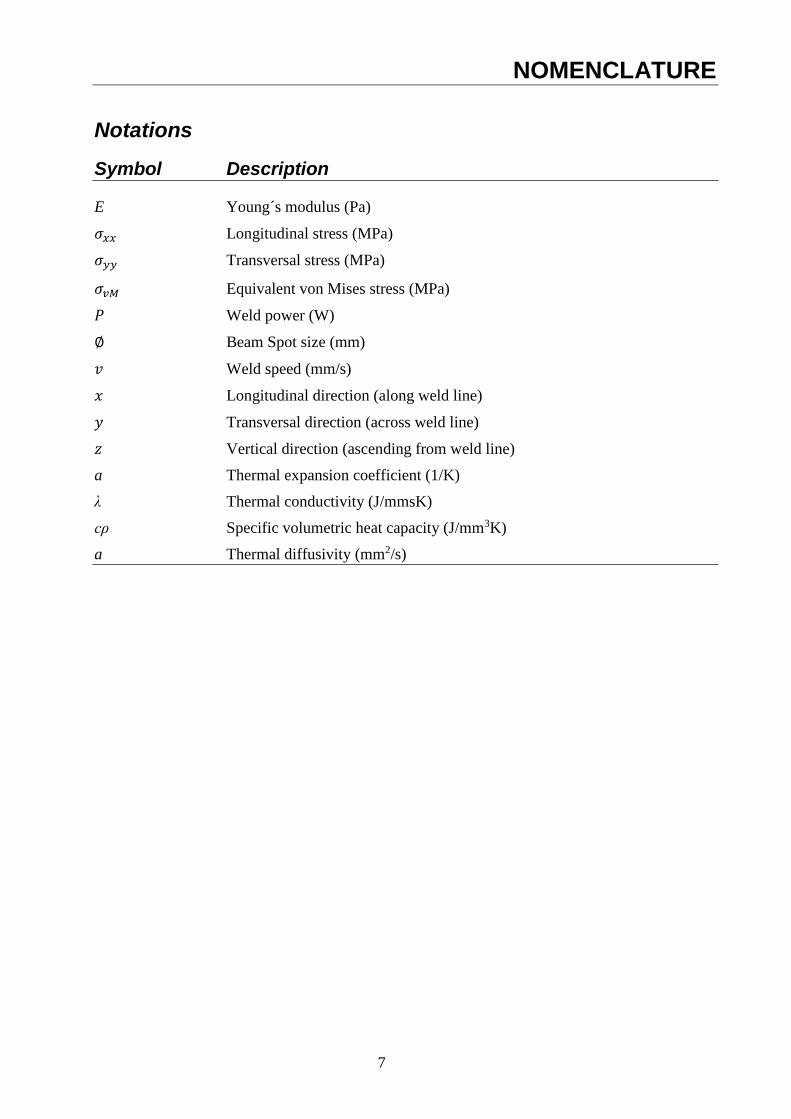
NOMENCLATURE
Notations
Symbol Description
E Young´s modulus (Pa)
𝜎𝑥𝑥 Longitudinal stress (MPa)
𝜎𝑦𝑦 Transversal stress (MPa)
𝜎𝑣𝑀 Equivalent von Mises stress (MPa)
𝑃 Weld power (W)
∅ Beam Spot size (mm)
𝑣 Weld speed (mm/s)
𝑥 Longitudinal direction (along weld line)
𝑦 Transversal direction (across weld line)
𝑧 Vertical direction (ascending from weld line)
a Thermal expansion coefficient (1/K)
λ Thermal conductivity (J/mmsK)
cρ Specific volumetric heat capacity (J/mm3K)
a Thermal diffusivity (mm2/s)
8
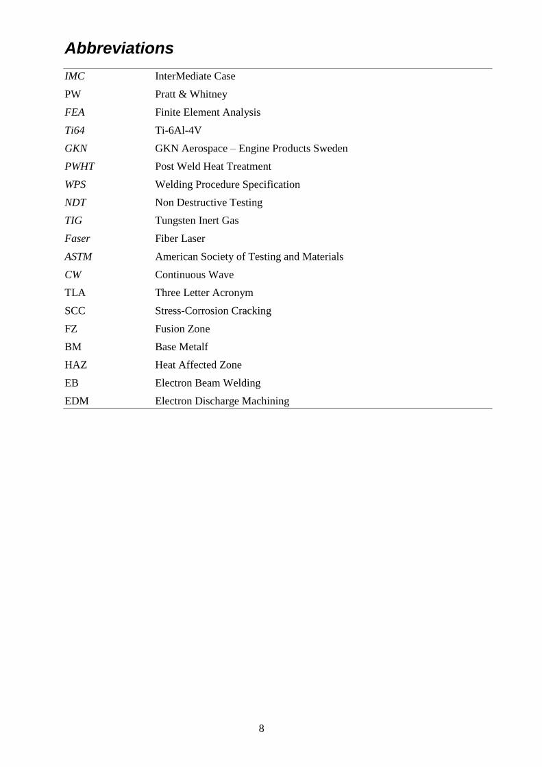
Abbreviations
IMC InterMediate Case
PW Pratt & Whitney
FEA Finite Element Analysis
Ti64 Ti-6Al-4V
GKN GKN Aerospace – Engine Products Sweden
PWHT Post Weld Heat Treatment
WPS Welding Procedure Specification
NDT Non Destructive Testing
TIG Tungsten Inert Gas
Faser Fiber Laser
ASTM American Society of Testing and Materials
CW Continuous Wave
TLA Three Letter Acronym
SCC Stress-Corrosion Cracking
FZ Fusion Zone
BM Base Metalf
HAZ Heat Affected Zone
EB Electron Beam Welding
EDM Electron Discharge Machining
9
TABLE OF CONTENTS
SAMMANFATTNING (SWEDISH)………………………………………………1
ABSTRACT.……………………………………………………………………….3
FOREWORD ............................................................................................................. 5
NOMENCLATURE .................................................................................................. 7
NOTATIONS ............................................................................................................. 7
TABLE OF CONTENTS .......................................................................................... 9
1 INTRODUCTION ............................................................................................ 12
1.1 BACKGROUND ............................................................................................ 12
1.2 PURPOSE ..................................................................................................... 14
1.3 PRELIMINARY HYPOTHESES ........................................................................ 15
1.4 DELIMITATIONS .......................................................................................... 15
1.5 METHOD ..................................................................................................... 16
1.6 RESEARCH QUESTIONS ................................................................................ 17
2 FRAME OF REFERENCE .............................................................................. 20
2.1 PREVIOUS WORK ......................................................................................... 20
2.2 TI-6AL-4V ................................................................................................. 23
2.3 THERMOMECHANICAL PROPERTIES ............................................................. 24
2.4 LASER WELDING ........................................................................................ 25
2.5 WELDING RESIDUAL STRESS ...................................................................... 28
2.6 RESIDUAL STRESS MEASUREMENT .............................................................. 32
2.7 STRESS-CORROSION CRACKING .................................................................. 33
2.8 TITANIUM ALPHA CASE ............................................................................... 33
2.9 WELDING SIMULATIONS .............................................................................. 34
2.10 STATE OF THE ART ...................................................................................... 35
3 IMPLEMENTATION ...................................................................................... 36
3.1 WELD GEOMETRY SET UP ............................................................................ 36
3.2 PARAMETER BOX SET UP ............................................................................. 37
3.3 WELDING .................................................................................................... 38
3.4 MICROGRAPHIC OBSERVATIONS.................................................................. 39
3.5 WELDING SIMULATIONS .............................................................................. 41
3.6 THERMAL MEASUREMENTS ........................................................................ 42
4 RESULTS ......................................................................................................... 44
4.1 THERMAL MEASUREMENTS ......................................................................... 44
4.2 WELDING SIMULATIONS .............................................................................. 44
5 DISCUSSION AND CONCLUSIONS ............................................................ 54
5.1 DISCUSSION ................................................................................................ 54
10
5.2 CONCLUSIONS ............................................................................................. 57
6 RECOMMENDATIONS AND FUTURE WORK .......................................... 58
6.1 RECOMMENDATIONS ................................................................................... 58
6.2 FUTURE WORK ............................................................................................ 58
7 REFERENCES ................................................................................................. 60
APPENDIX 1: WELD PARAMETERS & JOB NUMBERS ................................ 62
APPENDIX 2: WELD MICROGRAPHS .............................................................. 64
APPENDIX 3: STRESS EVOLUTION PLOTS .................................................... 72
APPENDIX 4: TEMPERATURE HISTORIES ..................................................... 76
APPENDIX 5: MAXIMUM TEMPERATURE PLOTS ........................................ 84
APPENDIX 6: MICRO LASER WELDING ......................................................... 88
APPENDIX 7: REFERENCE PICTURE OF AN IMC30K ................................... 90
APPENDIX 8: GANTT PLANNING CHART ...................................................... 92

11
12
1 INTRODUCTION
This section covers the underlying factors behind the need for repair welding, the reasons for
secrecy within the aerospace industry and by extension within this thesis, a purpose for this theses,
some preliminary hypotheses, delimitations of said hypotheses’ testing, a method for testing them,
and the research questions this thesis hopes to answer.
1.1 Background
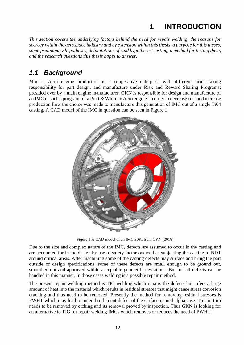
Modern Aero engine production is a cooperative enterprise with different firms taking
responsibility for part design, and manufacture under Risk and Reward Sharing Programs;
presided over by a main engine manufacturer. GKN is responsible for design and manufacture of
an IMC in such a program for a Pratt & Whitney Aero engine. In order to decrease cost and increase
production flow the choice was made to manufacture this generation of IMC out of a single Ti64
casting. A CAD model of the IMC in question can be seen in Figure 1
Figure 1 A CAD model of an IMC 30K, from GKN (2018)
Due to the size and complex nature of the IMC, defects are assumed to occur in the casting and
are accounted for in the design by use of safety factors as well as subjecting the casting to NDT
around critical areas. After machining some of the casting defects may surface and bring the part
outside of design specifications, some of these defects are small enough to be ground out,
smoothed out and approved within acceptable geometric deviations. But not all defects can be
handled in this manner, in those cases welding is a possible repair method.
The present repair welding method is TIG welding which repairs the defects but infers a large
amount of heat into the material which results in residual stresses that might cause stress corrosion
cracking and thus need to be removed. Presently the method for removing residual stresses is
PWHT which may lead to an embrittlement defect of the surface named alpha case. This in turn
needs to be removed by etching and its removal proved by inspection. Thus GKN is looking for
an alternative to TIG for repair welding IMCs which removes or reduces the need of PWHT.
13
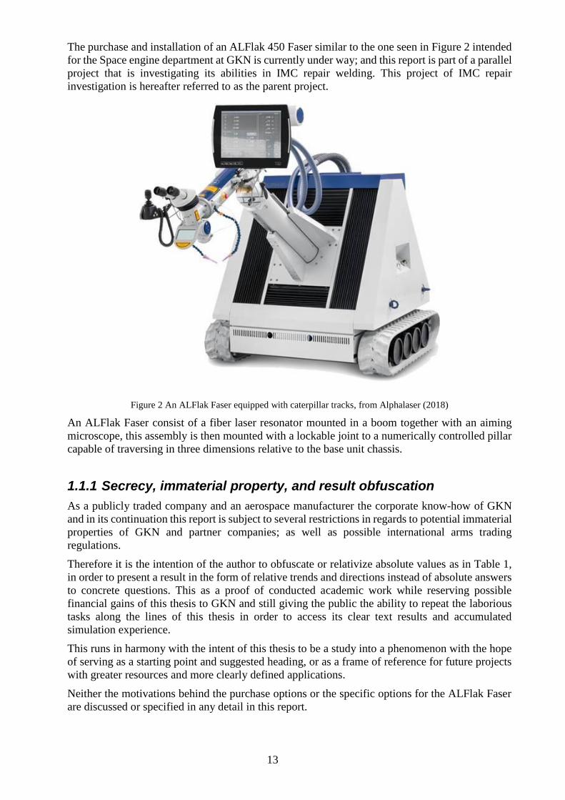
The purchase and installation of an ALFlak 450 Faser similar to the one seen in Figure 2 intended
for the Space engine department at GKN is currently under way; and this report is part of a parallel
project that is investigating its abilities in IMC repair welding. This project of IMC repair
investigation is hereafter referred to as the parent project.
Figure 2 An ALFlak Faser equipped with caterpillar tracks, from Alphalaser (2018)
An ALFlak Faser consist of a fiber laser resonator mounted in a boom together with an aiming
microscope, this assembly is then mounted with a lockable joint to a numerically controlled pillar
capable of traversing in three dimensions relative to the base unit chassis.
1.1.1 Secrecy, immaterial property, and result obfuscation
As a publicly traded company and an aerospace manufacturer the corporate know-how of GKN
and in its continuation this report is subject to several restrictions in regards to potential immaterial
properties of GKN and partner companies; as well as possible international arms trading
regulations.
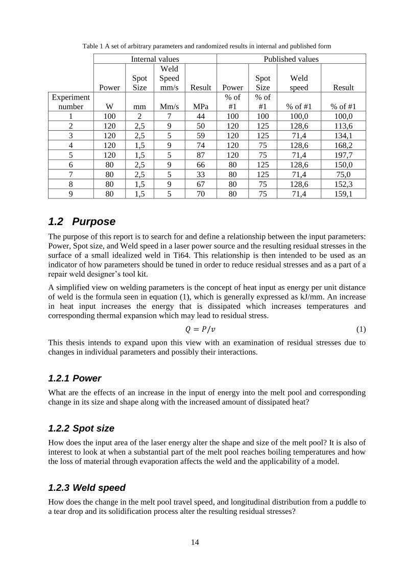
Therefore it is the intention of the author to obfuscate or relativize absolute values as in Table 1,
in order to present a result in the form of relative trends and directions instead of absolute answers
to concrete questions. This as a proof of conducted academic work while reserving possible
financial gains of this thesis to GKN and still giving the public the ability to repeat the laborious
tasks along the lines of this thesis in order to access its clear text results and accumulated
simulation experience.
This runs in harmony with the intent of this thesis to be a study into a phenomenon with the hope
of serving as a starting point and suggested heading, or as a frame of reference for future projects
with greater resources and more clearly defined applications.
Neither the motivations behind the purchase options or the specific options for the ALFlak Faser
are discussed or specified in any detail in this report.
14
Table 1 A set of arbitrary parameters and randomized results in internal and published form
Internal values Published values
Power
Spot
Size
Weld
Speed
mm/s Result Power
Spot
Size
Weld
speed Result
Experiment
number W mm Mm/s MPa
% of
#1
% of
#1 % of #1 % of #1
1 100 2 7 44 100 100 100,0 100,0
2 120 2,5 9 50 120 125 128,6 113,6
3 120 2,5 5 59 120 125 71,4 134,1
4 120 1,5 9 74 120 75 128,6 168,2
5 120 1,5 5 87 120 75 71,4 197,7
6 80 2,5 9 66 80 125 128,6 150,0
7 80 2,5 5 33 80 125 71,4 75,0
8 80 1,5 9 67 80 75 128,6 152,3
9 80 1,5 5 70 80 75 71,4 159,1
1.2 Purpose
The purpose of this report is to search for and define a relationship between the input parameters:
Power, Spot size, and Weld speed in a laser power source and the resulting residual stresses in the
surface of a small idealized weld in Ti64. This relationship is then intended to be used as an
indicator of how parameters should be tuned in order to reduce residual stresses and as a part of a
repair weld designer’s tool kit.
A simplified view on welding parameters is the concept of heat input as energy per unit distance
of weld is the formula seen in equation (1), which is generally expressed as kJ/mm. An increase
in heat input increases the energy that is dissipated which increases temperatures and
corresponding thermal expansion which may lead to residual stress.
𝑄 = 𝑃/𝑣 (1)
This thesis intends to expand upon this view with an examination of residual stresses due to
changes in individual parameters and possibly their interactions.
1.2.1 Power
What are the effects of an increase in the input of energy into the melt pool and corresponding
change in its size and shape along with the increased amount of dissipated heat?
1.2.2 Spot size
How does the input area of the laser energy alter the shape and size of the melt pool? It is also of
interest to look at when a substantial part of the melt pool reaches boiling temperatures and how
the loss of material through evaporation affects the weld and the applicability of a model.
1.2.3 Weld speed
How does the change in the melt pool travel speed, and longitudinal distribution from a puddle to
a tear drop and its solidification process alter the resulting residual stresses?
15
1.3 Preliminary hypotheses
1.3.1 Power
As Power is energy over time its increase should lead to increased weld pool temperatures which
in turn leads to a steeper thermal gradient resulting in a larger melt pool and a larger heated volume
of base material. This increase in affected volume is an increase in the amount of material that
takes part in the expansion and contraction of the thermal cycle, which are the main cause of
residual stresses in welding Ti64. Thus an increase in Power should lead to increased residual
stresses
1.3.2 Spot size
An increased Spot size distributes the welding energy over a larger area which should lower the
surface temperature of the weld pool while widening it and thus increasing the length of metal that
needs to contracts transversally to the weld line in a similar way to the effects of a Power increase.
1.3.3 Weld speed
An increase in Weld speed lowers the heat input but it also stretches the weld pool lengthwise,
assuming that the weld pool does not solidify immediately after the laser spot passes it. This
stretched solidification pattern means that the material solidifies and cools down faster and thus
has a shorter time so relieve itself in the longitudinal direction leading to higher residual stresses.
1.4 Delimitations
The following delimitations were made in order to reduce the scope to an area that is feasible for
the size of the assignment, coherent to the model being formulated, publishable without violations
of corporate secrecy, and practically feasible with the financial, computational, and intellectual
resources at hand.
• In the process of this thesis only Ti64 plates dimensioned 150X50X1mm (GKN Article
#156013) were simulated and welded.
• No actual residual stress measurements were made due to the cost of such measurements.
• All welds were made according to Figure 25 no filler material was added, nor was any joint
preparation performed apart from cleaning of the plates with acetone.
• Only parameter set ups that achieved a steady state weld bead were considered.
• Only parameter set ups that are possible in the ALFlak 450 were considered.
• No heed was taken to alpha case or other surface defects resulting from insufficient gas
shielding.
• All welds in this report, simulated and physical were made in the continuous weld mode in
order to achieve similarity between the actual weld, and the computer simulations.
16
1.5 Method
A method was proposed where the feasible weld geometry is defined, a box of interesting
parameters is set up, residual stresses are acquired, the response parameters are tested, and finally
a response model analysis is represented.
1.5.1 Weld geometry set up
In order to analyse a weld, a suitable weld geometry needs to be set up that takes heed of the needs
of both the scientific inquiry, and the general purpose that it sprung from. Out of these need the
following list of demands on the weld geometry was formulated.
1. Enabling acquirement of residual stresses.
2. Representability of a desired repair weld design.
3. Robustness in its physical application.
4. Feasibility to simulate.
5. Practical reproducibility in numbers.
6. Practical examinability under micrograph.
7. Practical measurability thermally.
1.5.2 Parameter box set up
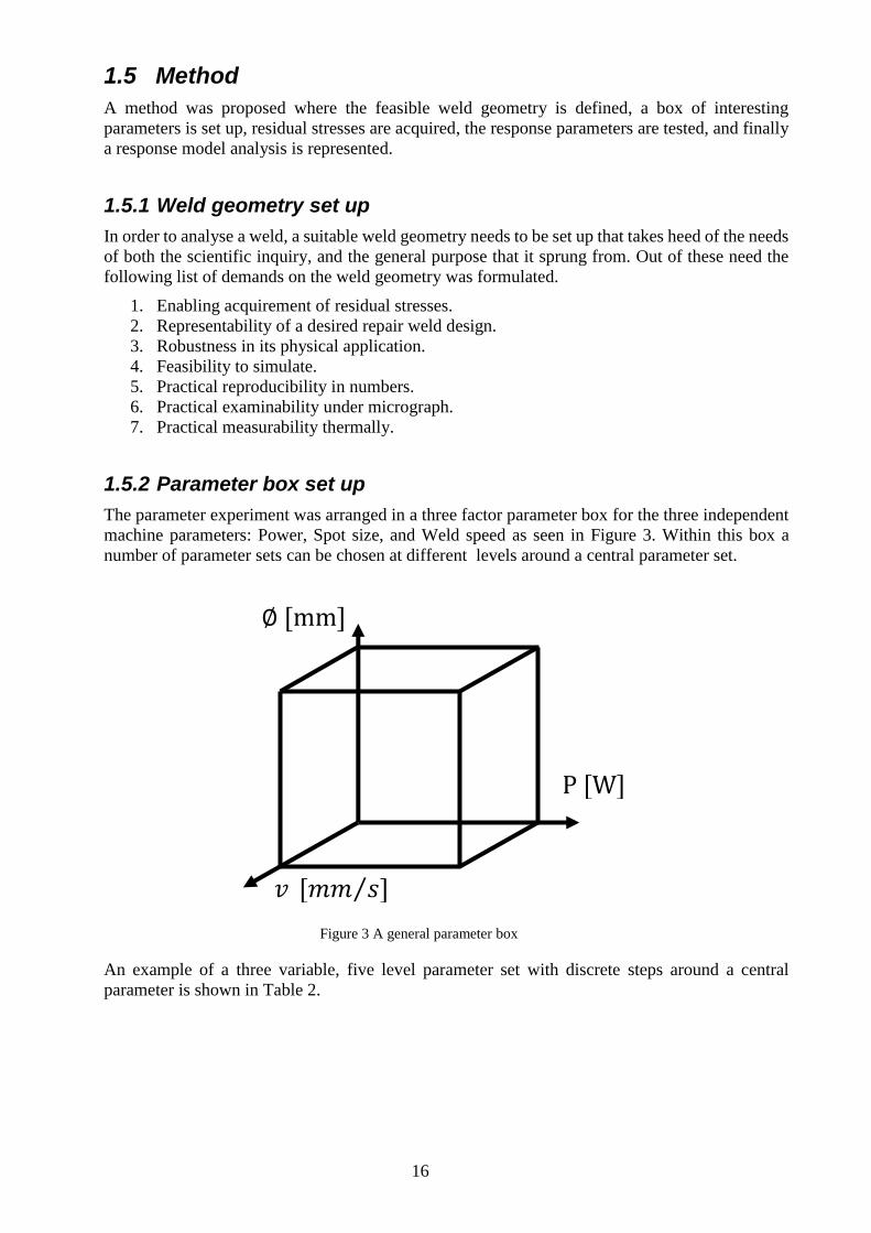
The parameter experiment was arranged in a three factor parameter box for the three independent
machine parameters: Power, Spot size, and Weld speed as seen in Figure 3. Within this box a
number of parameter sets can be chosen at different levels around a central parameter set.
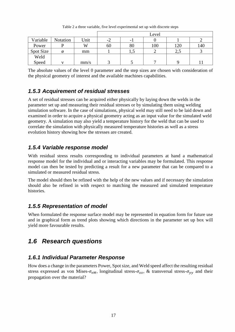
An example of a three variable, five level parameter set with discrete steps around a central
parameter is shown in Table 2.
P [W]
𝑣 [𝑚𝑚 𝑠]Τ
∅ [mm]
Figure 3 A general parameter box
17
Table 2 a three variable, five level experimental set up with discrete steps
Level
Variable Notation Unit -2 -1 0 1 2
Power P W 60 80 100 120 140
Spot Size ø mm 1 1,5 2 2,5 3
Weld
Speed v mm/s 3 5 7 9 11
The absolute values of the level 0 parameter and the step sizes are chosen with consideration of
the physical geometry of interest and the available machines capabilities.
1.5.3 Acquirement of residual stresses
A set of residual stresses can be acquired either physically by laying down the welds in the
parameter set up and measuring their residual stresses or by simulating them using welding
simulation software. In the case of simulations, physical weld may still need to be laid down and
examined in order to acquire a physical geometry acting as an input value for the simulated weld
geometry. A simulation may also yield a temperature history for the weld that can be used to
correlate the simulation with physically measured temperature histories as well as a stress
evolution history showing how the stresses are created.
1.5.4 Variable response model
With residual stress results corresponding to individual parameters at hand a mathematical
response model for the individual and or interacting variables may be formulated. This response
model can then be tested by predicting a result for a new parameter that can be compared to a
simulated or measured residual stress.
The model should then be refined with the help of the new values and if necessary the simulation
should also be refined in with respect to matching the measured and simulated temperature
histories.
1.5.5 Representation of model
When formulated the response surface model may be represented in equation form for future use
and in graphical form as trend plots showing which directions in the parameter set up box will
yield more favourable results.
1.6 Research questions
1.6.1 Individual Parameter Response
How does a change in the parameters Power, Spot size, and Weld speed affect the resulting residual
stress expressed as von Mises-𝜎𝑣𝑀, longitudinal stress-𝜎𝑥𝑥, & transversal stress-𝜎𝑦𝑦 and their
propagation over the material?
18
1.6.2 Synergetic Parameter Response
Are there any synergetic properties between the individual response parameters effect on the
resulting residual stress expressed as von Mises-𝜎𝑣𝑀, longitudinal stress-𝜎𝑥𝑥, & transversal stress-
𝜎𝑦𝑦 and their propagation over the material?

19
20
2 FRAME OF REFERENCE
This section covers previous work conducted within the parent project at GKN and in published
works, an overview of the properties of Ti64, the thermomechanical behavior of material
properties, an introduction to laser welding, a description of residual stresses and their genesis,
the measurement of residual stresses, problems pertinent to the parent project, the particulars of
welding simulation, as well as a description of the state of the art repair method
2.1 Previous work
2.1.1 GKN
As part of the parent project, a pre study with a YAG laser at a separate company in Bredaryd has
been conducted. This study was intended as a first grasp on the capabilities of Alphalaser’s product
line in order to compare its potential to the state of the art method TIG. Later equipment tests and
research welds were made with a representative 450 W Faser located at the reseller Stjernbergs
Automation in Kungsbacka; this in lieu of the ALFlak 450 Faser being procured. A set of precursor
weld coupons had also been sent to SWEREA IVF for neutron diffraction measurements of
residual stress. These measurements were deemed to be inconsequential in terms of values for this
report but helpful in where to start and informative on the subject in general.
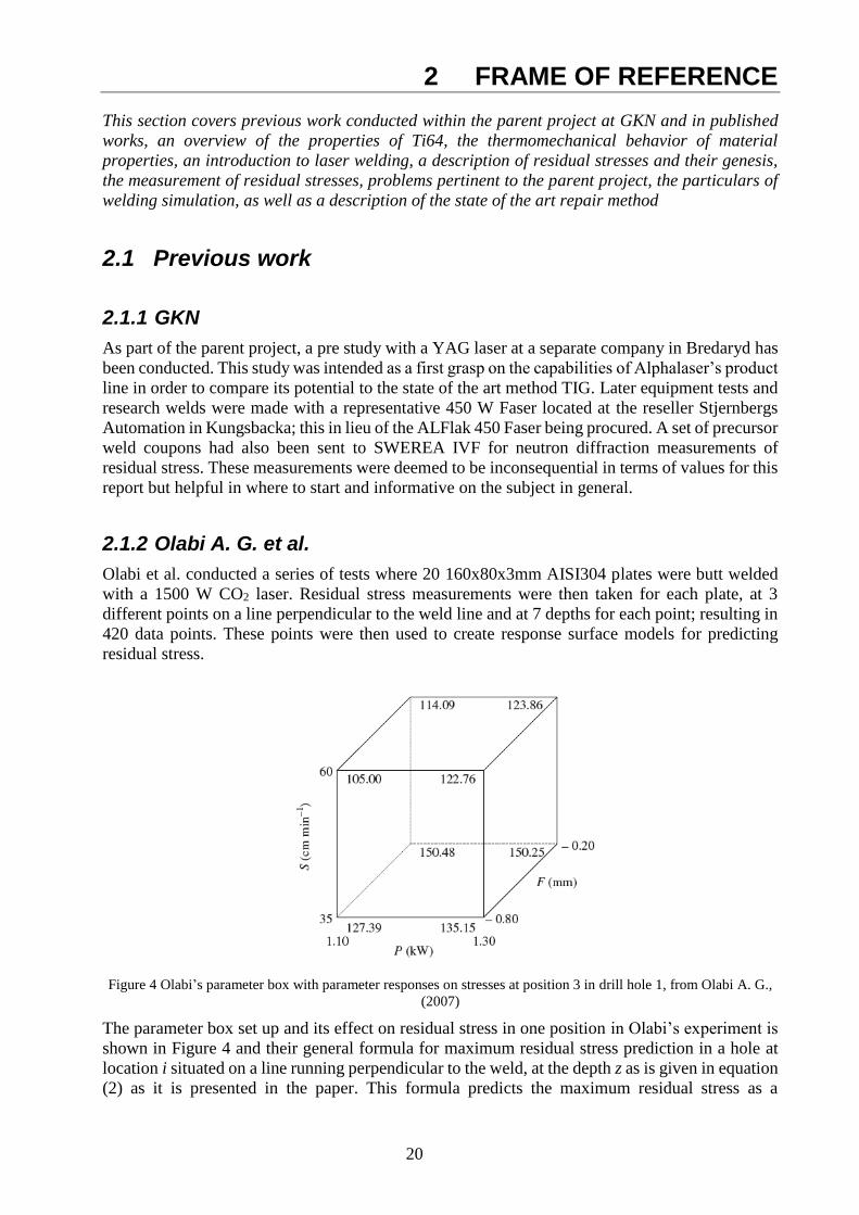
2.1.2 Olabi A. G. et al.
Olabi et al. conducted a series of tests where 20 160x80x3mm AISI304 plates were butt welded
with a 1500 W CO2 laser. Residual stress measurements were then taken for each plate, at 3
different points on a line perpendicular to the weld line and at 7 depths for each point; resulting in
420 data points. These points were then used to create response surface models for predicting
residual stress.
Figure 4 Olabi’s parameter box with parameter responses on stresses at position 3 in drill hole 1, from Olabi A. G.,
(2007)
The parameter box set up and its effect on residual stress in one position in Olabi’s experiment is
shown in Figure 4 and their general formula for maximum residual stress prediction in a hole at
location i situated on a line running perpendicular to the weld, at the depth z as is given in equation
(2) as it is presented in the paper. This formula predicts the maximum residual stress as a
21
polynomial with the coefficients b0-b33 corresponding to the factors Power (P), Weld speed (S),
and Focal height (F).
𝜎𝑖𝑧 = 𝑏0 + 𝑏1𝑃 + 𝑏2𝑆 + 𝑏3𝐹 + 𝑏11𝑃2 + 𝑏22𝑆2 + 𝑏33𝐹2 + 𝑏12𝑃𝑆 + 𝑏13𝑃𝐹 + 𝑏23𝑆𝐹 (2)
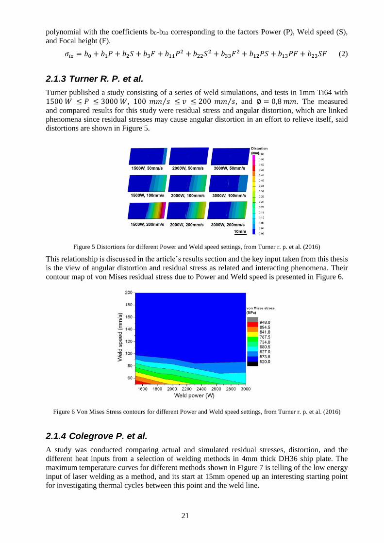
2.1.3 Turner R. P. et al.
Turner published a study consisting of a series of weld simulations, and tests in 1mm Ti64 with
1500 𝑊 ≤ 𝑃 ≤ 3000 𝑊, 100 𝑚𝑚 𝑠Τ ≤ 𝑣 ≤ 200 𝑚𝑚 𝑠Τ , and ∅ = 0,8 𝑚𝑚. The measured
and compared results for this study were residual stress and angular distortion, which are linked
phenomena since residual stresses may cause angular distortion in an effort to relieve itself, said
distortions are shown in Figure 5.
Figure 5 Distortions for different Power and Weld speed settings, from Turner r. p. et al. (2016)
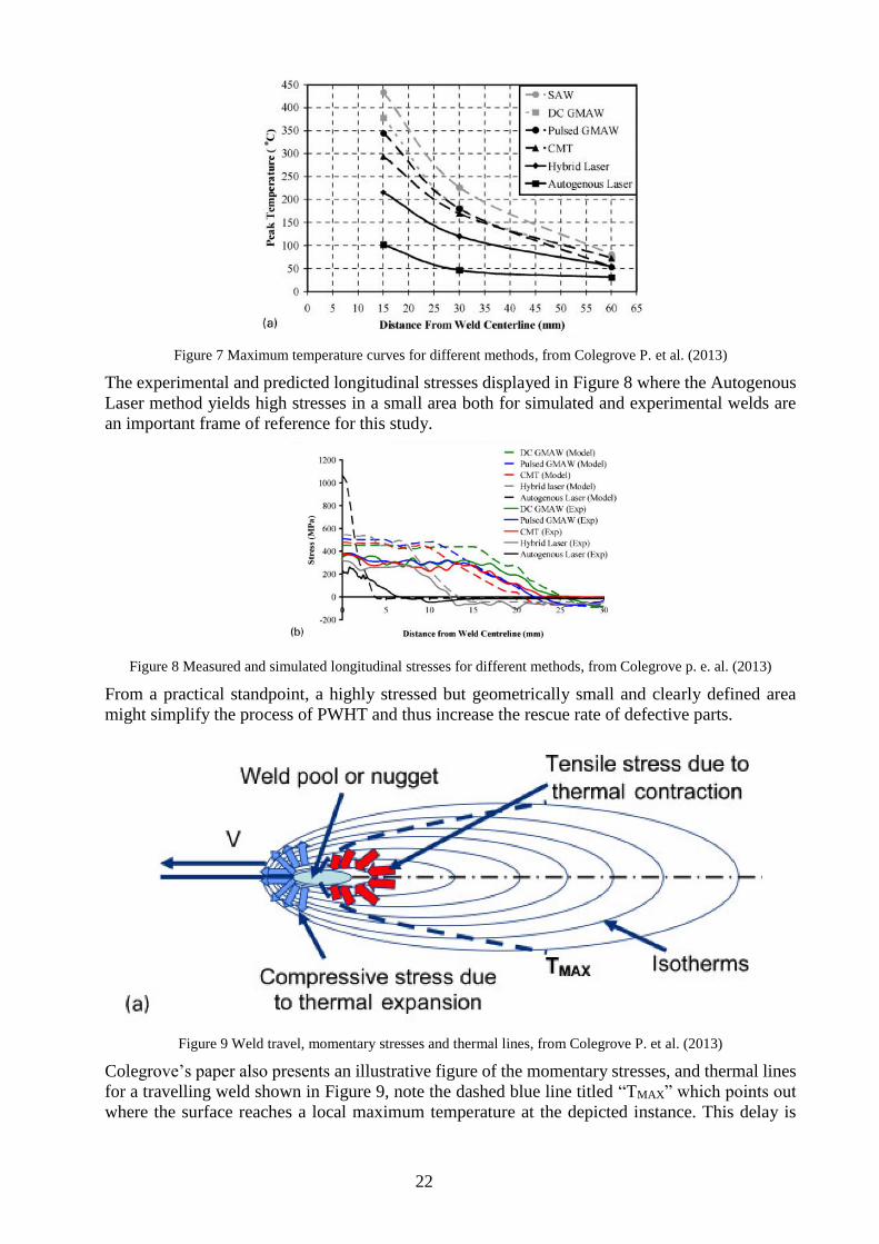
This relationship is discussed in the article’s results section and the key input taken from this thesis
is the view of angular distortion and residual stress as related and interacting phenomena. Their
contour map of von Mises residual stress due to Power and Weld speed is presented in Figure 6.
Figure 6 Von Mises Stress contours for different Power and Weld speed settings, from Turner r. p. et al. (2016)
2.1.4 Colegrove P. et al.
A study was conducted comparing actual and simulated residual stresses, distortion, and the
different heat inputs from a selection of welding methods in 4mm thick DH36 ship plate. The
maximum temperature curves for different methods shown in Figure 7 is telling of the low energy
input of laser welding as a method, and its start at 15mm opened up an interesting starting point
for investigating thermal cycles between this point and the weld line.
22
Figure 7 Maximum temperature curves for different methods, from Colegrove P. et al. (2013)
The experimental and predicted longitudinal stresses displayed in Figure 8 where the Autogenous
Laser method yields high stresses in a small area both for simulated and experimental welds are
an important frame of reference for this study.
Figure 8 Measured and simulated longitudinal stresses for different methods, from Colegrove p. e. al. (2013)
From a practical standpoint, a highly stressed but geometrically small and clearly defined area
might simplify the process of PWHT and thus increase the rescue rate of defective parts.
Figure 9 Weld travel, momentary stresses and thermal lines, from Colegrove P. et al. (2013)
Colegrove’s paper also presents an illustrative figure of the momentary stresses, and thermal lines
for a travelling weld shown in Figure 9, note the dashed blue line titled “TMAX” which points out
where the surface reaches a local maximum temperature at the depicted instance. This delay is
23
caused by the movement of the heat source and it is a three dimensional process stretching into the
material.
2.2 Ti-6Al-4V
Ti64 is an alpha-beta alloy of titanium, and the workhorse alloy of the titanium industry AZO
Materials (2018). With a minimum yield stress of 𝜎𝑦 = 897 𝑀𝑃𝑎 AZO materials (2018) it can be
compared strength wise to the high strength structural steel Strenx™ 900 with a yield stress
guaranteed to 𝜎𝑦 > 900 𝑀𝑃𝑎 SSAB (2018), this along its density of 𝜌𝑇𝑖 = 4420 𝑘𝑔/𝑚3
compared to pure Fe 𝜌𝐹𝑒 = 7874𝑘𝑔/𝑚3 Wikipedia (2018) makes the material switch from iron
to titanium in a design, yield a reduction in weight of about 44%.
Table 3 Elemental Composition of Ti-6Al-4V grade 5 according to ASTM B348 courtesy of Performance Titanium
Group (2018)
Element Ti Al V Fe O C N H
Quantity [%] Balance 5,5-
6,75
3,5-
4,5
≤0,4 ≤0,2 ≤0,08 ≤0,05 ≤0,012
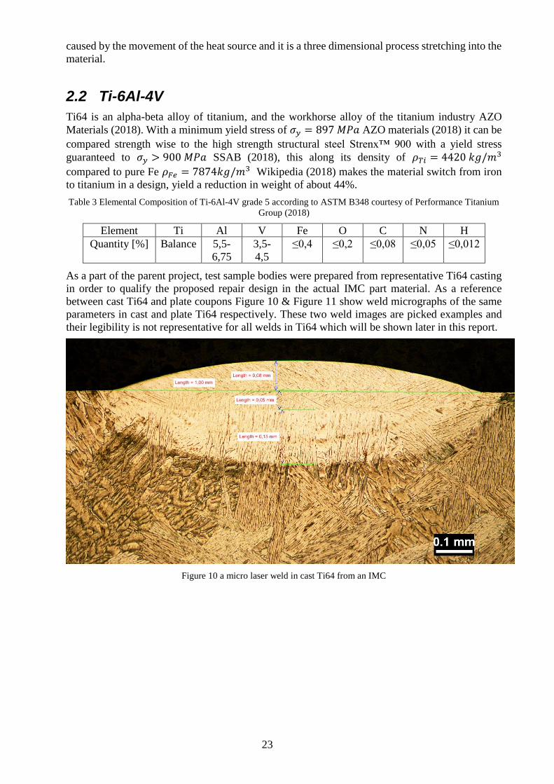
As a part of the parent project, test sample bodies were prepared from representative Ti64 casting
in order to qualify the proposed repair design in the actual IMC part material. As a reference
between cast Ti64 and plate coupons Figure 10 & Figure 11 show weld micrographs of the same
parameters in cast and plate Ti64 respectively. These two weld images are picked examples and
their legibility is not representative for all welds in Ti64 which will be shown later in this report.
Figure 10 a micro laser weld in cast Ti64 from an IMC
24
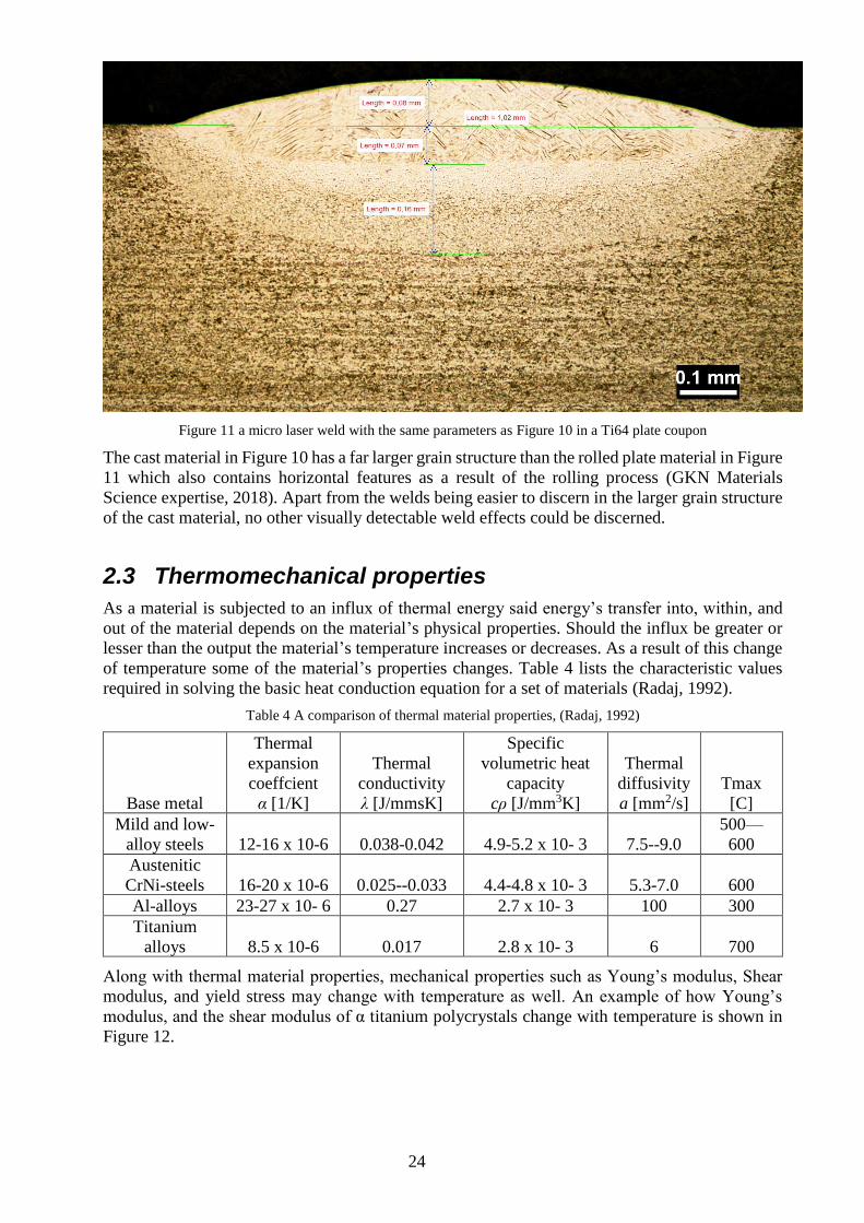
Figure 11 a micro laser weld with the same parameters as Figure 10 in a Ti64 plate coupon
The cast material in Figure 10 has a far larger grain structure than the rolled plate material in Figure
11 which also contains horizontal features as a result of the rolling process (GKN Materials
Science expertise, 2018). Apart from the welds being easier to discern in the larger grain structure
of the cast material, no other visually detectable weld effects could be discerned.
2.3 Thermomechanical properties
As a material is subjected to an influx of thermal energy said energy’s transfer into, within, and
out of the material depends on the material’s physical properties. Should the influx be greater or
lesser than the output the material’s temperature increases or decreases. As a result of this change
of temperature some of the material’s properties changes. Table 4 lists the characteristic values
required in solving the basic heat conduction equation for a set of materials (Radaj, 1992).
Table 4 A comparison of thermal material properties, (Radaj, 1992)
Base metal
Thermal
expansion
coeffcient
α [1/K]
Thermal
conductivity
λ [J/mmsK]
Specific
volumetric heat
capacity
cρ [J/mm3K]
Thermal
diffusivity
a [mm2/s]
Tmax
[C]
Mild and low-
alloy steels 12-16 x 10-6 0.038-0.042 4.9-5.2 x 10- 3 7.5--9.0
500—
600
Austenitic
CrNi-steels 16-20 x 10-6 0.025--0.033 4.4-4.8 x 10- 3 5.3-7.0 600
Al-alloys 23-27 x 10- 6 0.27 2.7 x 10- 3 100 300
Titanium
alloys 8.5 x 10⁻⁶ 0.017 2.8 x 10- 3 6 700
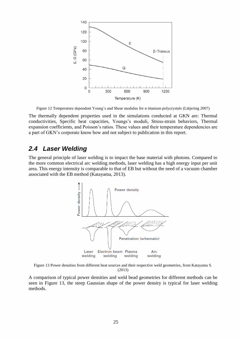
Along with thermal material properties, mechanical properties such as Young’s modulus, Shear
modulus, and yield stress may change with temperature as well. An example of how Young’s
modulus, and the shear modulus of α titanium polycrystals change with temperature is shown in
Figure 12.
25
Figure 12 Temperature dependent Young’s and Shear modulus for α titanium polycrystals (Lütjering 2007)
The thermally dependent properties used in the simulations conducted at GKN are: Thermal
conductivities, Specific heat capacities, Youngs’s moduli, Stress-strain behaviors, Thermal
expansion coefficients, and Poisson’s ratios. These values and their temperature dependencies are
a part of GKN’s corporate know how and not subject to publication in this report.
2.4 Laser Welding
The general principle of laser welding is to impact the base material with photons. Compared to
the more common electrical arc welding methods, laser welding has a high energy input per unit
area. This energy intensity is comparable to that of EB but without the need of a vacuum chamber
associated with the EB method (Katayama, 2013).
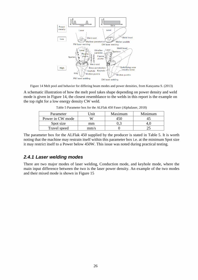
Figure 13 Power densities from different heat sources and their respective weld geometries, from Katayama S.
(2013)
A comparison of typical power densities and weld bead geometries for different methods can be
seen in Figure 13, the steep Gaussian shape of the power density is typical for laser welding
methods.
26
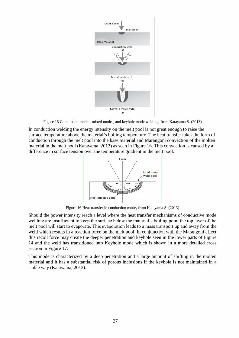
Figure 14 Melt pool and behavior for differing beam modes and power densities, from Katayama S. (2013)
A schematic illustration of how the melt pool takes shape depending on power density and weld
mode is given in Figure 14, the closest resemblance to the welds in this report is the example on
the top right for a low energy density CW weld.
Table 5 Parameter box for the ALFlak 450 Faser (Alphalaser, 2018)
Parameter Unit Maximum Minimum
Power in CW mode W 450 45
Spot size mm 0,3 4,0
Travel speed mm/s 0 25
The parameter box for the ALFlak 450 supplied by the producer is stated in Table 5. It is worth
noting that the machine may restrain itself within this parameter box i.e. at the minimum Spot size
it may restrict itself to a Power below 450W. This issue was noted during practical testing.
2.4.1 Laser welding modes
There are two major modes of laser welding, Conduction mode, and keyhole mode, where the
main input difference between the two is the laser power density. An example of the two modes
and their mixed mode is shown in Figure 15
27
Figure 15 Conduction mode-, mixed mode-, and keyhole mode welding, from Katayama S. (2013)
In conduction welding the energy intensity on the melt pool is not great enough to raise the
surface temperature above the material’s boiling temperature. The heat transfer takes the form of
conduction through the melt pool into the base material and Marangoni convection of the molten
material in the melt pool (Katayama, 2013) as seen in Figure 16. This convection is caused by a
difference in surface tension over the temperature gradient in the melt pool.
Figure 16 Heat transfer in conduction mode, from Katayama S. (2013)
Should the power intensity reach a level where the heat transfer mechanisms of conductive mode
welding are insufficient to keep the surface below the material’s boiling point the top layer of the
melt pool will start to evaporate. This evaporation leads to a mass transport up and away from the
weld which results in a reaction force on the melt pool. In conjunction with the Marangoni effect
this recoil force may create the deeper penetration and keyhole seen in the lower parts of Figure
14 and the weld has transitioned into Keyhole mode which is shown in a more detailed cross
section in Figure 17.
This mode is characterized by a deep penetration and a large amount of shifting in the molten
material and it has a substantial risk of porous inclusions if the keyhole is not maintained in a
stable way (Katayama, 2013).
28
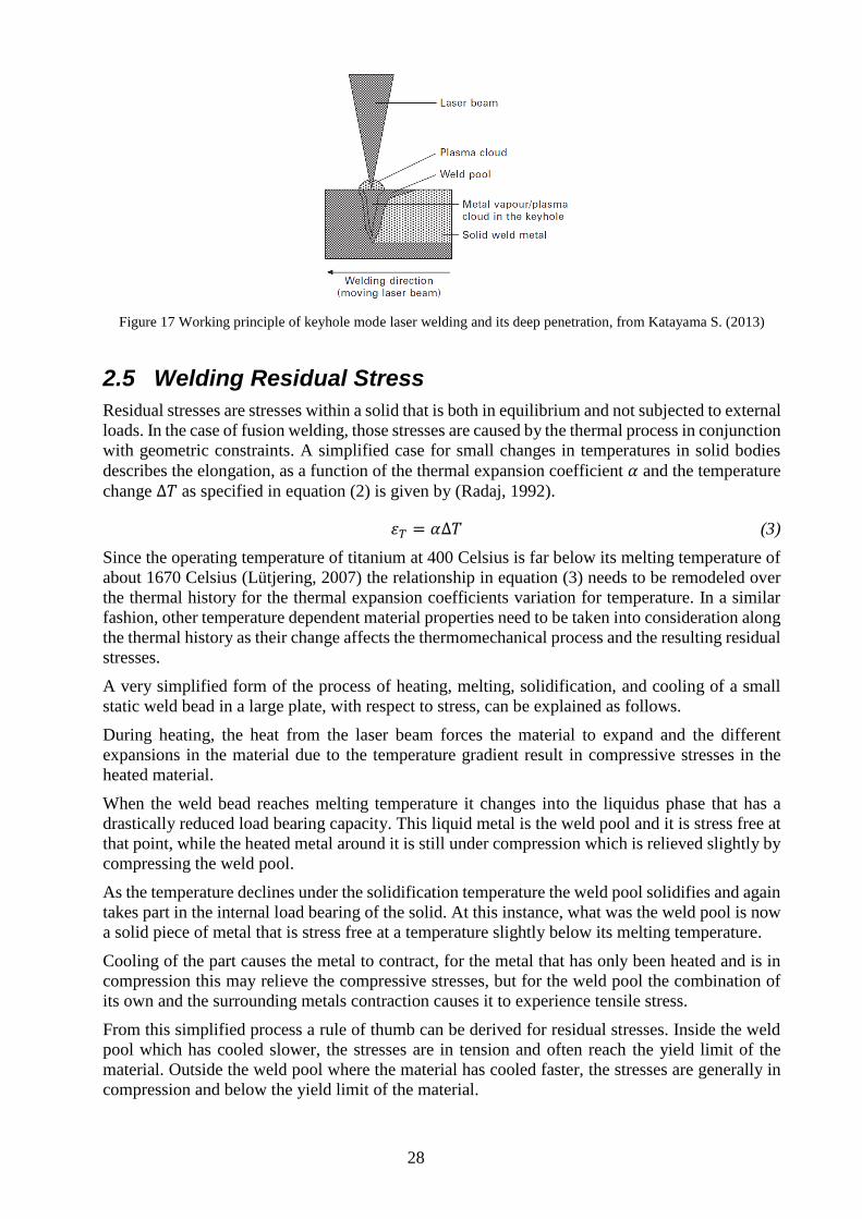
Figure 17 Working principle of keyhole mode laser welding and its deep penetration, from Katayama S. (2013)
2.5 Welding Residual Stress
Residual stresses are stresses within a solid that is both in equilibrium and not subjected to external
loads. In the case of fusion welding, those stresses are caused by the thermal process in conjunction
with geometric constraints. A simplified case for small changes in temperatures in solid bodies
describes the elongation, as a function of the thermal expansion coefficient 𝛼 and the temperature
change ∆𝑇 as specified in equation (2) is given by (Radaj, 1992).
𝜀𝑇 = 𝛼∆𝑇 (3)
Since the operating temperature of titanium at 400 Celsius is far below its melting temperature of
about 1670 Celsius (Lütjering, 2007) the relationship in equation (3) needs to be remodeled over
the thermal history for the thermal expansion coefficients variation for temperature. In a similar
fashion, other temperature dependent material properties need to be taken into consideration along
the thermal history as their change affects the thermomechanical process and the resulting residual
stresses.
A very simplified form of the process of heating, melting, solidification, and cooling of a small
static weld bead in a large plate, with respect to stress, can be explained as follows.
During heating, the heat from the laser beam forces the material to expand and the different
expansions in the material due to the temperature gradient result in compressive stresses in the
heated material.
When the weld bead reaches melting temperature it changes into the liquidus phase that has a
drastically reduced load bearing capacity. This liquid metal is the weld pool and it is stress free at
that point, while the heated metal around it is still under compression which is relieved slightly by
compressing the weld pool.
As the temperature declines under the solidification temperature the weld pool solidifies and again
takes part in the internal load bearing of the solid. At this instance, what was the weld pool is now
a solid piece of metal that is stress free at a temperature slightly below its melting temperature.
Cooling of the part causes the metal to contract, for the metal that has only been heated and is in
compression this may relieve the compressive stresses, but for the weld pool the combination of
its own and the surrounding metals contraction causes it to experience tensile stress.
From this simplified process a rule of thumb can be derived for residual stresses. Inside the weld
pool which has cooled slower, the stresses are in tension and often reach the yield limit of the
material. Outside the weld pool where the material has cooled faster, the stresses are generally in
compression and below the yield limit of the material.
29
Further factors complicating the determination of residual stresses include but are not exclusively:
welding speed, weld width, weld penetration, weld length, weld geometry, addition of filler
materials, part fixturing, heat dissipation flows, temperature dependent elemental properties, phase
dependent material properties etc. Thus a FEA approach to solving residual stresses in welds more
complex than idealized simple geometries may be preferred over an analytical approach.
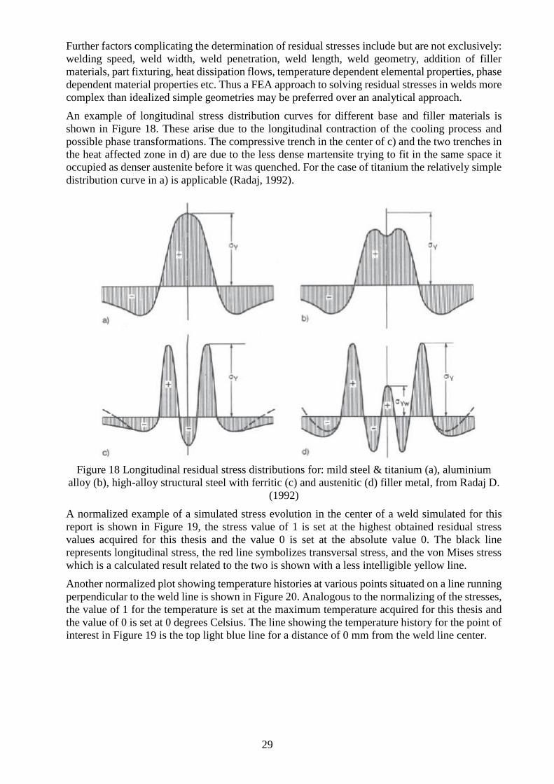
An example of longitudinal stress distribution curves for different base and filler materials is
shown in Figure 18. These arise due to the longitudinal contraction of the cooling process and
possible phase transformations. The compressive trench in the center of c) and the two trenches in
the heat affected zone in d) are due to the less dense martensite trying to fit in the same space it
occupied as denser austenite before it was quenched. For the case of titanium the relatively simple
distribution curve in a) is applicable (Radaj, 1992).
Figure 18 Longitudinal residual stress distributions for: mild steel & titanium (a), aluminium
alloy (b), high-alloy structural steel with ferritic (c) and austenitic (d) filler metal, from Radaj D.
(1992)
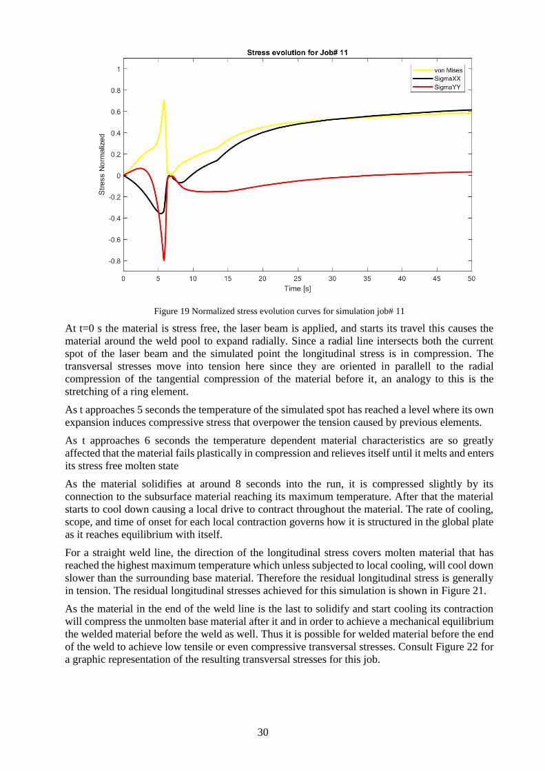
A normalized example of a simulated stress evolution in the center of a weld simulated for this
report is shown in Figure 19, the stress value of 1 is set at the highest obtained residual stress
values acquired for this thesis and the value 0 is set at the absolute value 0. The black line
represents longitudinal stress, the red line symbolizes transversal stress, and the von Mises stress
which is a calculated result related to the two is shown with a less intelligible yellow line.
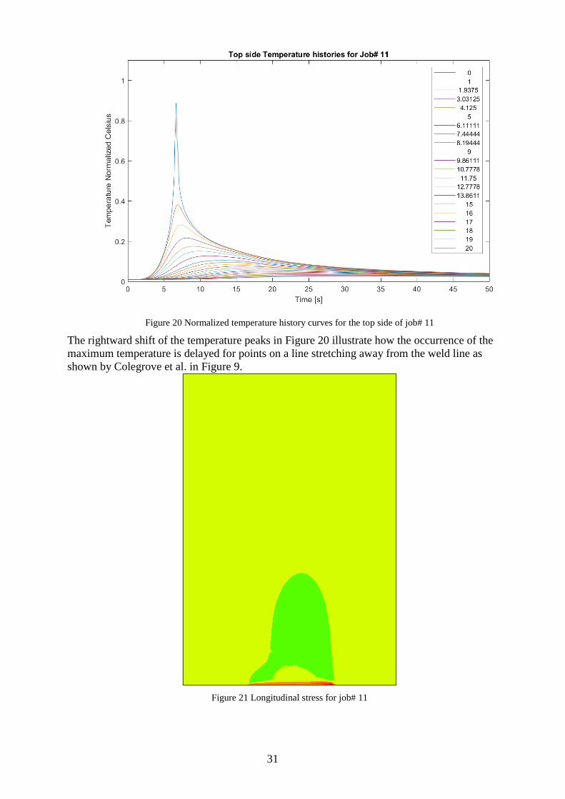
Another normalized plot showing temperature histories at various points situated on a line running
perpendicular to the weld line is shown in Figure 20. Analogous to the normalizing of the stresses,
the value of 1 for the temperature is set at the maximum temperature acquired for this thesis and
the value of 0 is set at 0 degrees Celsius. The line showing the temperature history for the point of
interest in Figure 19 is the top light blue line for a distance of 0 mm from the weld line center.
30
Figure 19 Normalized stress evolution curves for simulation job# 11
At t=0 s the material is stress free, the laser beam is applied, and starts its travel this causes the
material around the weld pool to expand radially. Since a radial line intersects both the current
spot of the laser beam and the simulated point the longitudinal stress is in compression. The
transversal stresses move into tension here since they are oriented in parallell to the radial
compression of the tangential compression of the material before it, an analogy to this is the
stretching of a ring element.
As t approaches 5 seconds the temperature of the simulated spot has reached a level where its own
expansion induces compressive stress that overpower the tension caused by previous elements.
As t approaches 6 seconds the temperature dependent material characteristics are so greatly
affected that the material fails plastically in compression and relieves itself until it melts and enters
its stress free molten state
As the material solidifies at around 8 seconds into the run, it is compressed slightly by its
connection to the subsurface material reaching its maximum temperature. After that the material
starts to cool down causing a local drive to contract throughout the material. The rate of cooling,
scope, and time of onset for each local contraction governs how it is structured in the global plate
as it reaches equilibrium with itself.
For a straight weld line, the direction of the longitudinal stress covers molten material that has
reached the highest maximum temperature which unless subjected to local cooling, will cool down
slower than the surrounding base material. Therefore the residual longitudinal stress is generally
in tension. The residual longitudinal stresses achieved for this simulation is shown in Figure 21.
As the material in the end of the weld line is the last to solidify and start cooling its contraction
will compress the unmolten base material after it and in order to achieve a mechanical equilibrium
the welded material before the weld as well. Thus it is possible for welded material before the end
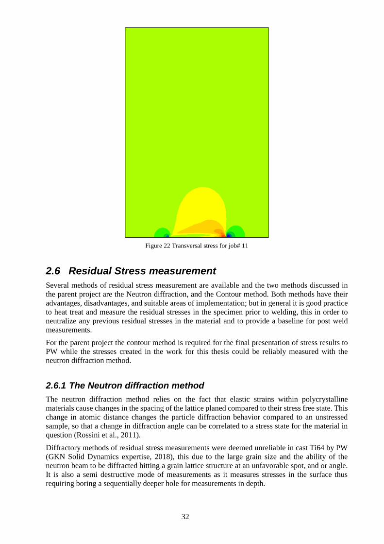
of the weld to achieve low tensile or even compressive transversal stresses. Consult Figure 22 for
a graphic representation of the resulting transversal stresses for this job.
31
Figure 20 Normalized temperature history curves for the top side of job# 11
The rightward shift of the temperature peaks in Figure 20 illustrate how the occurrence of the
maximum temperature is delayed for points on a line stretching away from the weld line as
shown by Colegrove et al. in Figure 9.
Figure 21 Longitudinal stress for job# 11
32
Figure 22 Transversal stress for job# 11
2.6 Residual Stress measurement
Several methods of residual stress measurement are available and the two methods discussed in
the parent project are the Neutron diffraction, and the Contour method. Both methods have their
advantages, disadvantages, and suitable areas of implementation; but in general it is good practice
to heat treat and measure the residual stresses in the specimen prior to welding, this in order to
neutralize any previous residual stresses in the material and to provide a baseline for post weld
measurements.
For the parent project the contour method is required for the final presentation of stress results to
PW while the stresses created in the work for this thesis could be reliably measured with the
neutron diffraction method.
2.6.1 The Neutron diffraction method
The neutron diffraction method relies on the fact that elastic strains within polycrystalline
materials cause changes in the spacing of the lattice planed compared to their stress free state. This
change in atomic distance changes the particle diffraction behavior compared to an unstressed
sample, so that a change in diffraction angle can be correlated to a stress state for the material in
question (Rossini et al., 2011).
Diffractory methods of residual stress measurements were deemed unreliable in cast Ti64 by PW
(GKN Solid Dynamics expertise, 2018), this due to the large grain size and the ability of the
neutron beam to be diffracted hitting a grain lattice structure at an unfavorable spot, and or angle.
It is also a semi destructive mode of measurements as it measures stresses in the surface thus
requiring boring a sequentially deeper hole for measurements in depth.
33
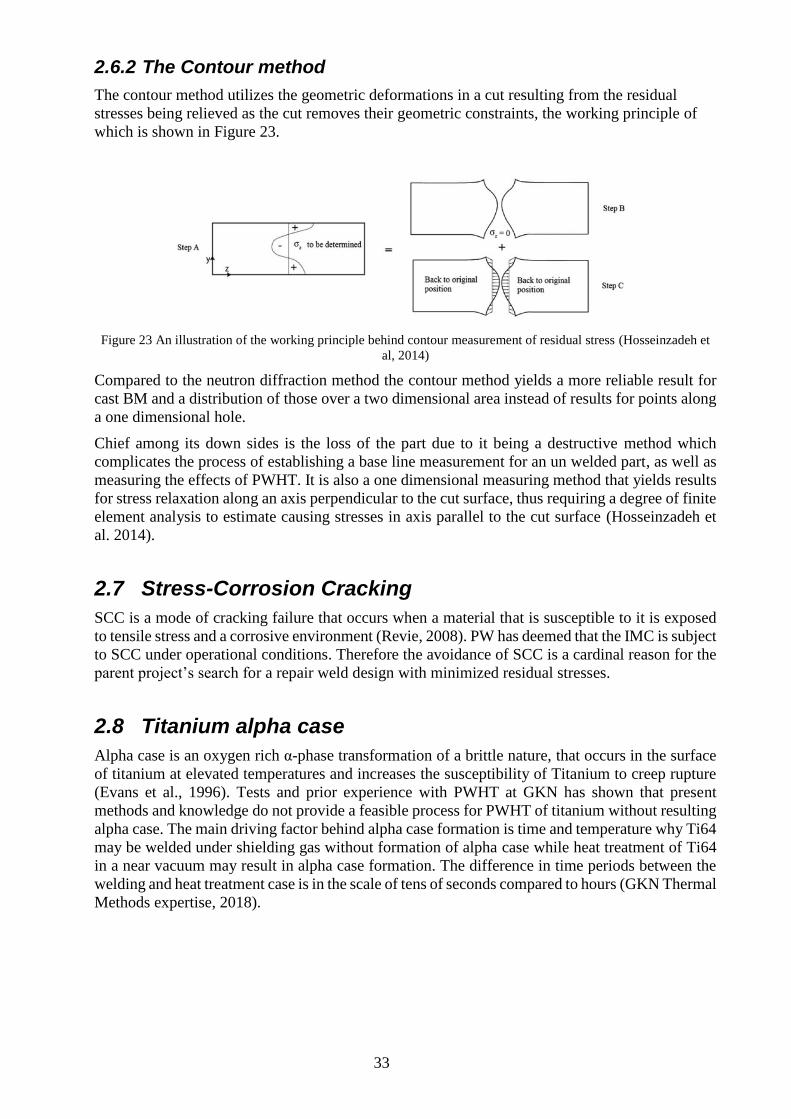
2.6.2 The Contour method
The contour method utilizes the geometric deformations in a cut resulting from the residual
stresses being relieved as the cut removes their geometric constraints, the working principle of
which is shown in Figure 23.
Figure 23 An illustration of the working principle behind contour measurement of residual stress (Hosseinzadeh et
al, 2014)
Compared to the neutron diffraction method the contour method yields a more reliable result for
cast BM and a distribution of those over a two dimensional area instead of results for points along
a one dimensional hole.
Chief among its down sides is the loss of the part due to it being a destructive method which
complicates the process of establishing a base line measurement for an un welded part, as well as
measuring the effects of PWHT. It is also a one dimensional measuring method that yields results
for stress relaxation along an axis perpendicular to the cut surface, thus requiring a degree of finite
element analysis to estimate causing stresses in axis parallel to the cut surface (Hosseinzadeh et
al. 2014).
2.7 Stress-Corrosion Cracking
SCC is a mode of cracking failure that occurs when a material that is susceptible to it is exposed
to tensile stress and a corrosive environment (Revie, 2008). PW has deemed that the IMC is subject
to SCC under operational conditions. Therefore the avoidance of SCC is a cardinal reason for the
parent project’s search for a repair weld design with minimized residual stresses.
2.8 Titanium alpha case
Alpha case is an oxygen rich α-phase transformation of a brittle nature, that occurs in the surface
of titanium at elevated temperatures and increases the susceptibility of Titanium to creep rupture
(Evans et al., 1996). Tests and prior experience with PWHT at GKN has shown that present
methods and knowledge do not provide a feasible process for PWHT of titanium without resulting
alpha case. The main driving factor behind alpha case formation is time and temperature why Ti64
may be welded under shielding gas without formation of alpha case while heat treatment of Ti64
in a near vacuum may result in alpha case formation. The difference in time periods between the
welding and heat treatment case is in the scale of tens of seconds compared to hours (GKN Thermal
Methods expertise, 2018).
34
2.9 Welding simulations
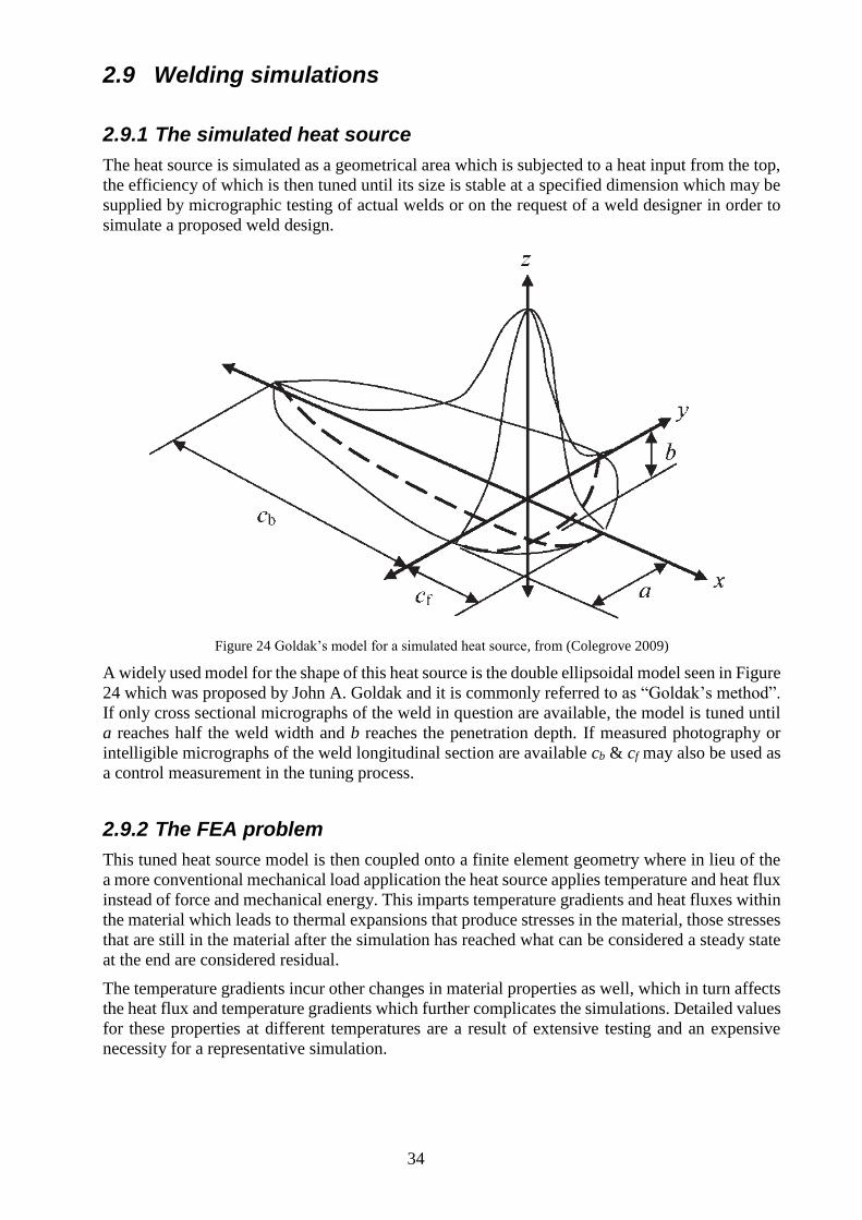
2.9.1 The simulated heat source
The heat source is simulated as a geometrical area which is subjected to a heat input from the top,
the efficiency of which is then tuned until its size is stable at a specified dimension which may be
supplied by micrographic testing of actual welds or on the request of a weld designer in order to
simulate a proposed weld design.
Figure 24 Goldak’s model for a simulated heat source, from (Colegrove 2009)
A widely used model for the shape of this heat source is the double ellipsoidal model seen in Figure
24 which was proposed by John A. Goldak and it is commonly referred to as “Goldak’s method”.
If only cross sectional micrographs of the weld in question are available, the model is tuned until
a reaches half the weld width and b reaches the penetration depth. If measured photography or
intelligible micrographs of the weld longitudinal section are available cb & cf may also be used as
a control measurement in the tuning process.
2.9.2 The FEA problem
This tuned heat source model is then coupled onto a finite element geometry where in lieu of the
a more conventional mechanical load application the heat source applies temperature and heat flux
instead of force and mechanical energy. This imparts temperature gradients and heat fluxes within
the material which leads to thermal expansions that produce stresses in the material, those stresses
that are still in the material after the simulation has reached what can be considered a steady state
at the end are considered residual.
The temperature gradients incur other changes in material properties as well, which in turn affects
the heat flux and temperature gradients which further complicates the simulations. Detailed values
for these properties at different temperatures are a result of extensive testing and an expensive
necessity for a representative simulation.
35
2.9.3 Boundary values
As with a physical weld the stresses in a simulated weld exert and relieve themselves on the base
material in the form of distortions. This may lead to a two part answer consisting of both residual
stresses and the deformations exerted by them. Therefore it is important to impose boundary value
conditions so that the searched for residual stresses are not relieved by their resulting deformations.
Although it is also important not to apply too strenuous boundary conditions as the geometry needs
to be able to deform in order to yield realistic residual stresses as well as to go through a realistic
thermal expansion/contraction process. A finer mesh lessens this problem but is more computer
intensive thus the expert’s judgement of the simulation engineer is required to balance this
problem.
2.10 State of the art
Presently at GKN, small repair welds are prepared by grinding out the defects with a rotary file
before they are filled up by the TIG method in a low Power setting, by continuously feeding filler
material into the melt pool. This is a wholly manual method using an arc light heat source which
requires the operator to use a welding mask and possibly gloves. The maintenance of a stable TIG
arc also requires a certain weld current and voltage which results in a higher input into the weld.
Compared to the TIG method the micro laser method is a gloves off operation conducted through
an aiming microscope with minimal emissions of visible light disturbing the observation of the
weld. Laser welding also has the capability of delivering a specific energy quantum in pulses
without the need to establish and maintain an arc as for traditional arc welding methods.
36
3 IMPLEMENTATION
This section covers the actual weld geometry set up, the parameter box’s set up, the test welding
procedure, micrographic observations of the welds, simulation of the measured weld geometries,
and thermal measurements of select welds.
3.1 Weld geometry set up
Following the demands stated in 1.5.1 a pertinent weld geometry was set up along the
considerations of the stated demands, and the practical implementations.
Residual stress measurements of physical welds were found to require individual coupons for each
weld that would at the least need to be heat treated, welded, and measured for residual stresses at
least in the post weld state. The total cost of which would land in the 100 000 SEK range, which
was deemed too expensive for this report. Therefore the choice was made to only acquire residual
stresses via simulation and to order the weld set up with respect to that purpose.
As stated earlier a physical state of the art repair weld consists of a small ground out hole that is
filled up with filler wire. This process is not applicable in welding simulation due to the need of
adding mesh elements and reshaping the mesh in simulation of added filler material which is
extremely computer intensive (GKN Welding Simulation expertise, 2018). Also a possible future
repair design was proposed; wherein the surface is of the crack is left unground and then laser
welded with a WPS that is proven to yield sufficient penetration. Thus an autogenous weld was
chosen i.e. no filler wire was added.
The hemispherical nature of the present repair weld would also lead to a complicated pattern in
the simulation with the laser doing PWHT on earlier welds which might yield inconclusive results
in the simulation. A circular or helical shape weld is also more practically complex to program
into the welding machine and semi automate wherefore a straight weld bead was chosen.
Measuring plate surface temperature during ALFlak welding with a thermal camera is problematic
due to its near infrared wavelength of 1070 nm (Alphalaser, 2018) interfering with the imaging
(GKN Method Engineering expertise, 2018) Thus a weld line of 20mm was chosen. It was deemed
long enough to be measured while passing a thermocouple of the K-type used at GKN, but not as
long as to require too large a simulation or, amount of test plates.
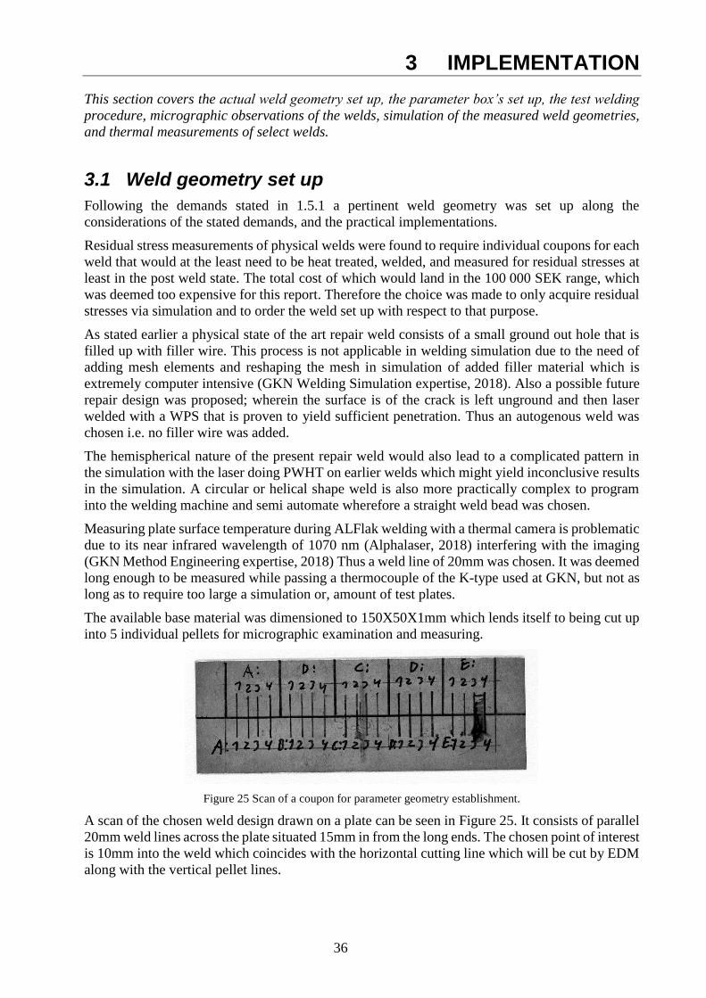
The available base material was dimensioned to 150X50X1mm which lends itself to being cut up
into 5 individual pellets for micrographic examination and measuring.
Figure 25 Scan of a coupon for parameter geometry establishment.
A scan of the chosen weld design drawn on a plate can be seen in Figure 25. It consists of parallel
20mm weld lines across the plate situated 15mm in from the long ends. The chosen point of interest
is 10mm into the weld which coincides with the horizontal cutting line which will be cut by EDM
along with the vertical pellet lines.
37
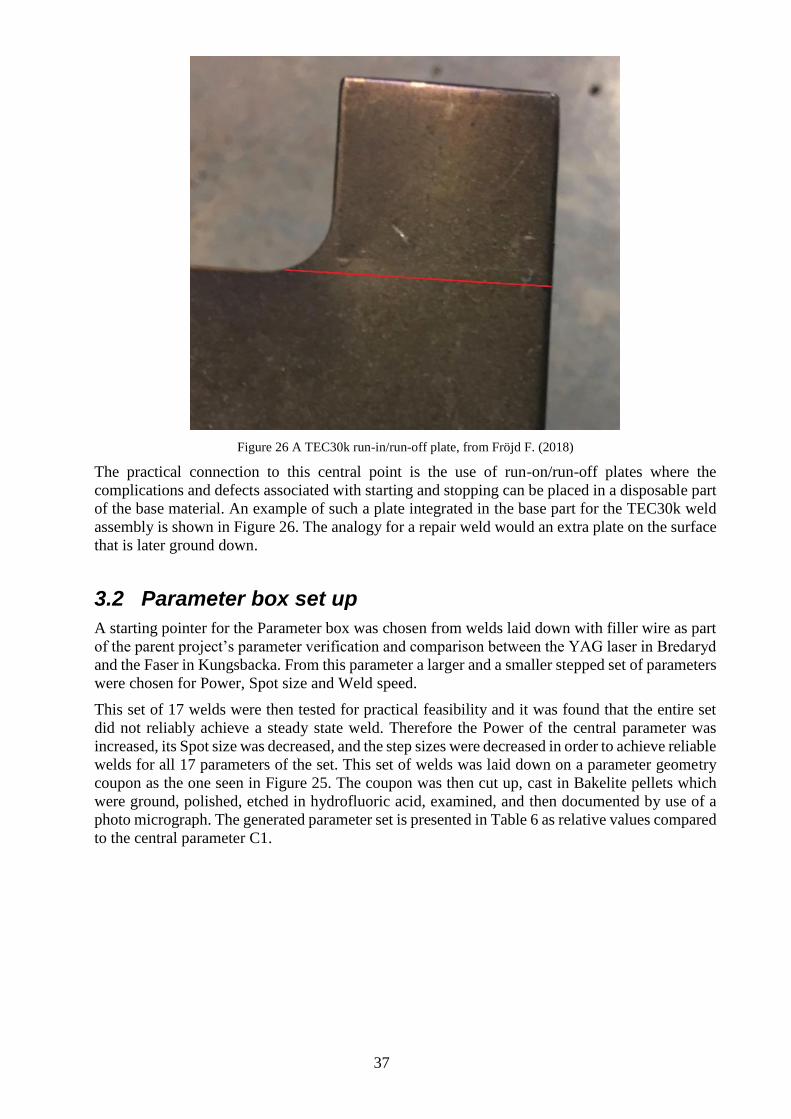
Figure 26 A TEC30k run-in/run-off plate, from Fröjd F. (2018)
The practical connection to this central point is the use of run-on/run-off plates where the
complications and defects associated with starting and stopping can be placed in a disposable part
of the base material. An example of such a plate integrated in the base part for the TEC30k weld
assembly is shown in Figure 26. The analogy for a repair weld would an extra plate on the surface
that is later ground down.
3.2 Parameter box set up
A starting pointer for the Parameter box was chosen from welds laid down with filler wire as part
of the parent project’s parameter verification and comparison between the YAG laser in Bredaryd
and the Faser in Kungsbacka. From this parameter a larger and a smaller stepped set of parameters
were chosen for Power, Spot size and Weld speed.
This set of 17 welds were then tested for practical feasibility and it was found that the entire set
did not reliably achieve a steady state weld. Therefore the Power of the central parameter was
increased, its Spot size was decreased, and the step sizes were decreased in order to achieve reliable
welds for all 17 parameters of the set. This set of welds was laid down on a parameter geometry
coupon as the one seen in Figure 25. The coupon was then cut up, cast in Bakelite pellets which
were ground, polished, etched in hydrofluoric acid, examined, and then documented by use of a
photo micrograph. The generated parameter set is presented in Table 6 as relative values compared
to the central parameter C1.
38
Table 6 Normalized parameter set for weld geometry investigation
Pellet # P [% of C1] ø [% of C1] v [% of C1]
A
1 108,3 125 120
2 108,3 125 80
3 108,3 75 120
4 108,3 75 80
B
1 91,7 125 120
2 91,7 125 80
3 91,7 75 120
4 91,7 75 80
C 1 100,0 100 100
D
1 116,7 150 140
2 116,7 150 60
3 116,7 50 140
4 116,7 50 60
E
1 83,3 150 140
2 83,3 150 60
3 83,3 50 140
4 83,3 50 60
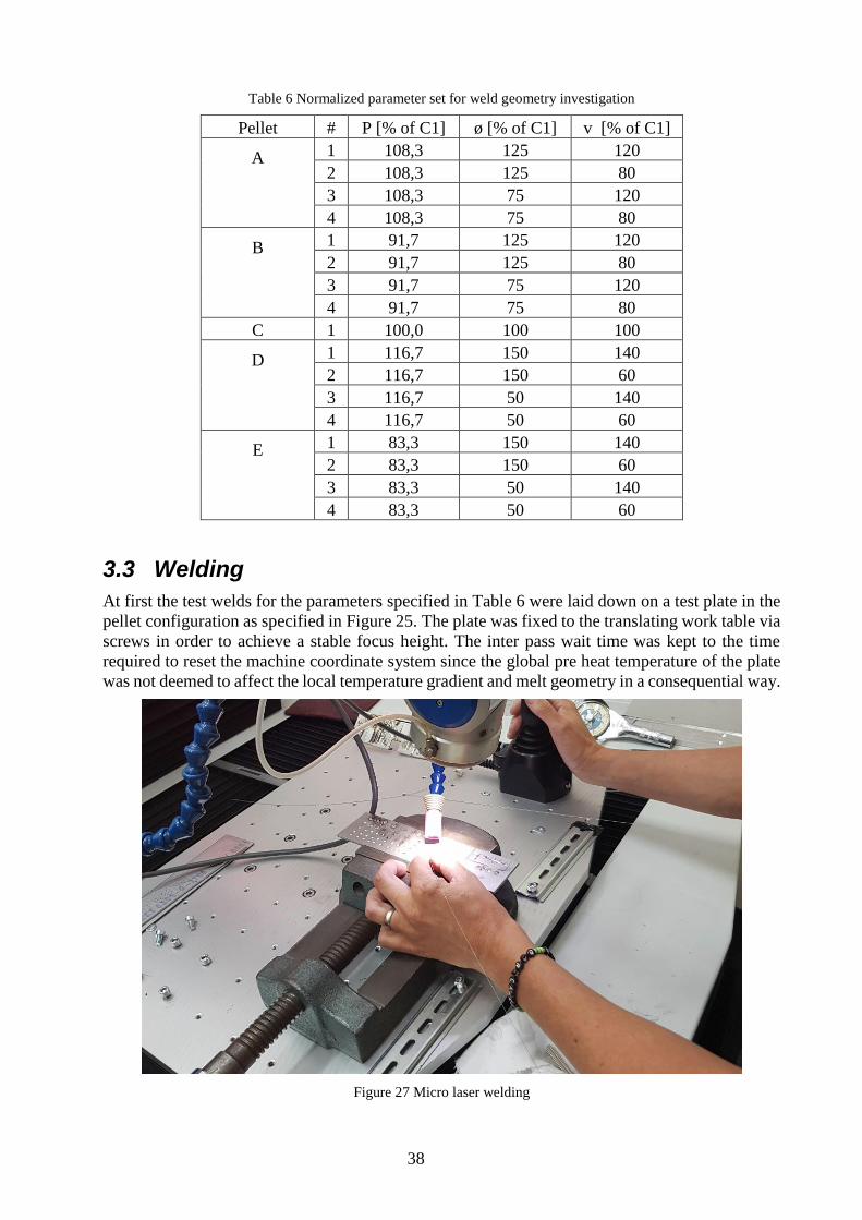
3.3 Welding
At first the test welds for the parameters specified in Table 6 were laid down on a test plate in the
pellet configuration as specified in Figure 25. The plate was fixed to the translating work table via
screws in order to achieve a stable focus height. The inter pass wait time was kept to the time
required to reset the machine coordinate system since the global pre heat temperature of the plate
was not deemed to affect the local temperature gradient and melt geometry in a consequential way.
Figure 27 Micro laser welding
39
A detail view of representative micro laser welding that is part of the parent project is shown in
Figure 27 and a larger uncropped version of the same image can be found in APPENDIX 6 for
reference.
3.4 Micrographic observations
All micrographic pictures in this chapter are set to the same “x m” reference bar unless otherwise
specified.
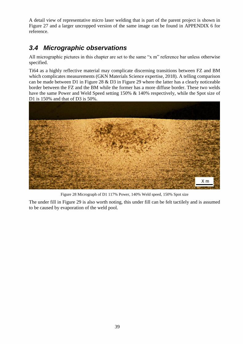
Ti64 as a highly reflective material may complicate discerning transitions between FZ and BM
which complicates measurements (GKN Materials Science expertise, 2018). A telling comparison
can be made between D1 in Figure 28 & D3 in Figure 29 where the latter has a clearly noticeable
border between the FZ and the BM while the former has a more diffuse border. These two welds
have the same Power and Weld Speed setting 150% & 140% respectively, while the Spot size of
D1 is 150% and that of D3 is 50%.
Figure 28 Micrograph of D1 117% Power, 140% Weld speed, 150% Spot size
The under fill in Figure 29 is also worth noting, this under fill can be felt tactilely and is assumed
to be caused by evaporation of the weld pool.
40
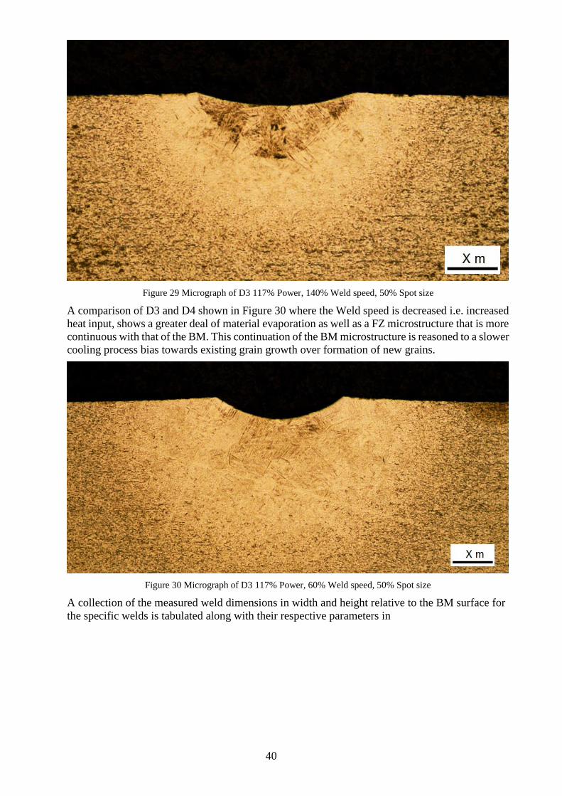
Figure 29 Micrograph of D3 117% Power, 140% Weld speed, 50% Spot size
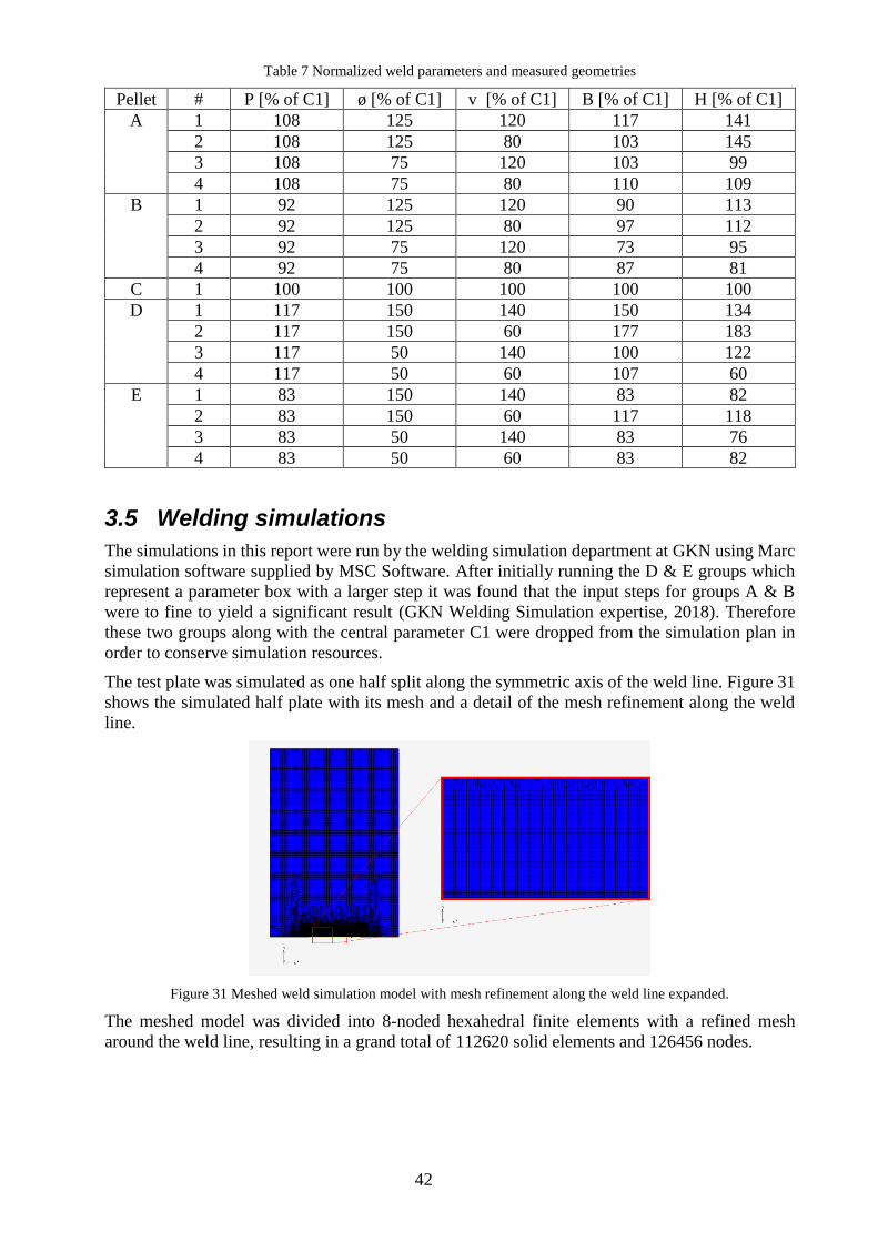
A comparison of D3 and D4 shown in Figure 30 where the Weld speed is decreased i.e. increased
heat input, shows a greater deal of material evaporation as well as a FZ microstructure that is more
continuous with that of the BM. This continuation of the BM microstructure is reasoned to a slower
cooling process bias towards existing grain growth over formation of new grains.
Figure 30 Micrograph of D3 117% Power, 60% Weld speed, 50% Spot size
A collection of the measured weld dimensions in width and height relative to the BM surface for
the specific welds is tabulated along with their respective parameters in

41
Table 7 and are used in the next chapter to size the weld pool in the simulations. This table and
all the weld micrographs are collected in APPENDIX 2.
42
Table 7 Normalized weld parameters and measured geometries
Pellet # P [% of C1] ø [% of C1] v [% of C1] B [% of C1] H [% of C1]
A 1 108 125 120 117 141
2 108 125 80 103 145
3 108 75 120 103 99
4 108 75 80 110 109
B 1 92 125 120 90 113
2 92 125 80 97 112
3 92 75 120 73 95
4 92 75 80 87 81
C 1 100 100 100 100 100
D 1 117 150 140 150 134
2 117 150 60 177 183
3 117 50 140 100 122
4 117 50 60 107 60
E 1 83 150 140 83 82
2 83 150 60 117 118
3 83 50 140 83 76
4 83 50 60 83 82
3.5 Welding simulations
The simulations in this report were run by the welding simulation department at GKN using Marc
simulation software supplied by MSC Software. After initially running the D & E groups which
represent a parameter box with a larger step it was found that the input steps for groups A & B
were to fine to yield a significant result (GKN Welding Simulation expertise, 2018). Therefore
these two groups along with the central parameter C1 were dropped from the simulation plan in
order to conserve simulation resources.
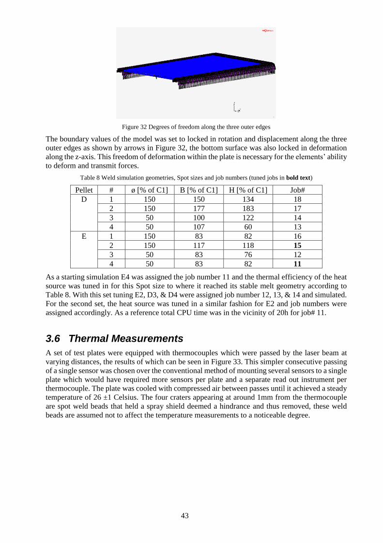
The test plate was simulated as one half split along the symmetric axis of the weld line. Figure 31
shows the simulated half plate with its mesh and a detail of the mesh refinement along the weld
line.
Figure 31 Meshed weld simulation model with mesh refinement along the weld line expanded.
The meshed model was divided into 8-noded hexahedral finite elements with a refined mesh
around the weld line, resulting in a grand total of 112620 solid elements and 126456 nodes.
43
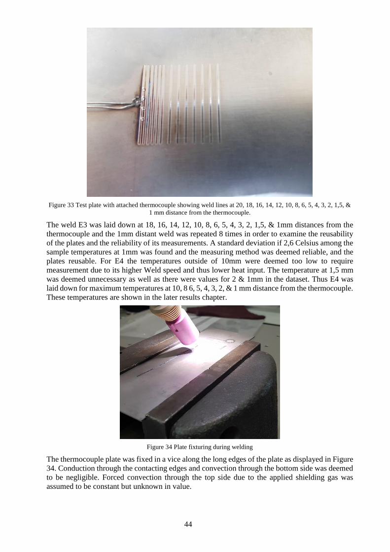
Figure 32 Degrees of freedom along the three outer edges
The boundary values of the model was set to locked in rotation and displacement along the three
outer edges as shown by arrows in Figure 32, the bottom surface was also locked in deformation
along the z-axis. This freedom of deformation within the plate is necessary for the elements’ ability
to deform and transmit forces.
Table 8 Weld simulation geometries, Spot sizes and job numbers (tuned jobs in bold text)
Pellet # ø [% of C1] B [% of C1] H [% of C1] Job#
D 1 150 150 134 18
2 150 177 183 17
3 50 100 122 14
4 50 107 60 13
E 1 150 83 82 16
2 150 117 118 15
3 50 83 76 12
4 50 83 82 11
As a starting simulation E4 was assigned the job number 11 and the thermal efficiency of the heat
source was tuned in for this Spot size to where it reached its stable melt geometry according to
Table 8. With this set tuning E2, D3, & D4 were assigned job number 12, 13, & 14 and simulated.
For the second set, the heat source was tuned in a similar fashion for E2 and job numbers were
assigned accordingly. As a reference total CPU time was in the vicinity of 20h for job# 11.
3.6 Thermal Measurements
A set of test plates were equipped with thermocouples which were passed by the laser beam at
varying distances, the results of which can be seen in Figure 33. This simpler consecutive passing
of a single sensor was chosen over the conventional method of mounting several sensors to a single
plate which would have required more sensors per plate and a separate read out instrument per
thermocouple. The plate was cooled with compressed air between passes until it achieved a steady
temperature of 26 ±1 Celsius. The four craters appearing at around 1mm from the thermocouple
are spot weld beads that held a spray shield deemed a hindrance and thus removed, these weld
beads are assumed not to affect the temperature measurements to a noticeable degree.
44
Figure 33 Test plate with attached thermocouple showing weld lines at 20, 18, 16, 14, 12, 10, 8, 6, 5, 4, 3, 2, 1,5, &
1 mm distance from the thermocouple.
The weld E3 was laid down at 18, 16, 14, 12, 10, 8, 6, 5, 4, 3, 2, 1,5, & 1mm distances from the
thermocouple and the 1mm distant weld was repeated 8 times in order to examine the reusability
of the plates and the reliability of its measurements. A standard deviation if 2,6 Celsius among the
sample temperatures at 1mm was found and the measuring method was deemed reliable, and the
plates reusable. For E4 the temperatures outside of 10mm were deemed too low to require
measurement due to its higher Weld speed and thus lower heat input. The temperature at 1,5 mm
was deemed unnecessary as well as there were values for 2 & 1mm in the dataset. Thus E4 was
laid down for maximum temperatures at 10, 8 6, 5, 4, 3, 2, & 1 mm distance from the thermocouple.
These temperatures are shown in the later results chapter.
Figure 34 Plate fixturing during welding
The thermocouple plate was fixed in a vice along the long edges of the plate as displayed in Figure
34. Conduction through the contacting edges and convection through the bottom side was deemed
to be negligible. Forced convection through the top side due to the applied shielding gas was
assumed to be constant but unknown in value.
45
4 RESULTS
This section covers and partially presents the results from: the thermal measurements, and the
welding simulations in stresses, temperature histories, as well as maximum temperatures,
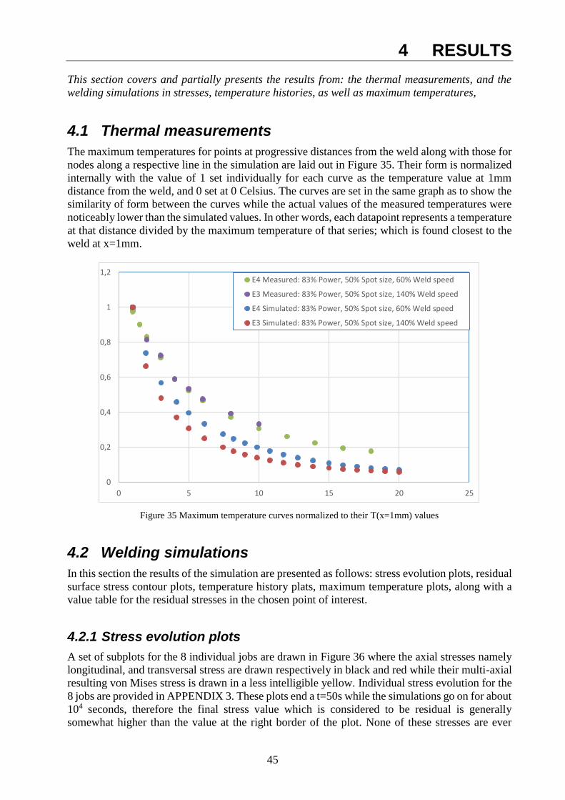
4.1 Thermal measurements
The maximum temperatures for points at progressive distances from the weld along with those for
nodes along a respective line in the simulation are laid out in Figure 35. Their form is normalized
internally with the value of 1 set individually for each curve as the temperature value at 1mm
distance from the weld, and 0 set at 0 Celsius. The curves are set in the same graph as to show the
similarity of form between the curves while the actual values of the measured temperatures were
noticeably lower than the simulated values. In other words, each datapoint represents a temperature
at that distance divided by the maximum temperature of that series; which is found closest to the
weld at x=1mm.
Figure 35 Maximum temperature curves normalized to their T(x=1mm) values
4.2 Welding simulations
In this section the results of the simulation are presented as follows: stress evolution plots, residual
surface stress contour plots, temperature history plats, maximum temperature plots, along with a
value table for the residual stresses in the chosen point of interest.
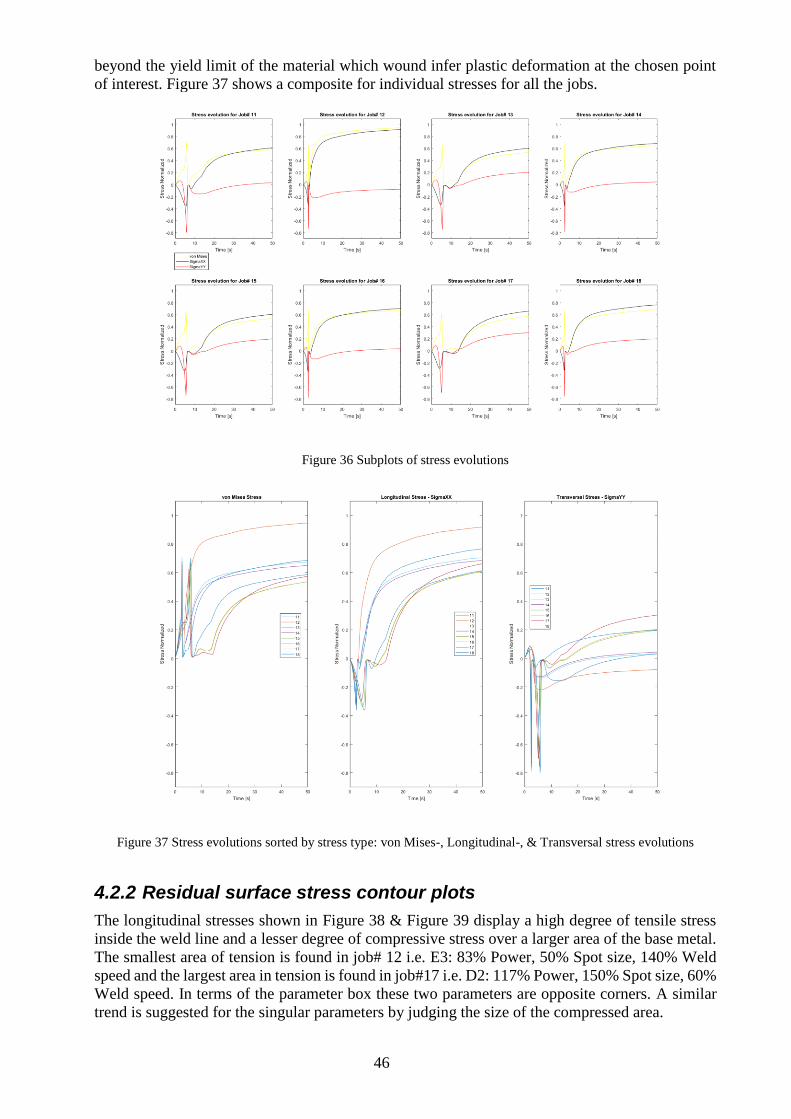
4.2.1 Stress evolution plots
A set of subplots for the 8 individual jobs are drawn in Figure 36 where the axial stresses namely
longitudinal, and transversal stress are drawn respectively in black and red while their multi-axial
resulting von Mises stress is drawn in a less intelligible yellow. Individual stress evolution for the
8 jobs are provided in APPENDIX 3. These plots end a t=50s while the simulations go on for about
104 seconds, therefore the final stress value which is considered to be residual is generally
somewhat higher than the value at the right border of the plot. None of these stresses are ever
0
0,2
0,4
0,6
0,8
1
1,2
0 5 10 15 20 25
E4 Measured: 83% Power, 50% Spot size, 60% Weld speed
E3 Measured: 83% Power, 50% Spot size, 140% Weld speed
E4 Simulated: 83% Power, 50% Spot size, 60% Weld speed
E3 Simulated: 83% Power, 50% Spot size, 140% Weld speed
46
beyond the yield limit of the material which wound infer plastic deformation at the chosen point
of interest. Figure 37 shows a composite for individual stresses for all the jobs.
Figure 36 Subplots of stress evolutions
Figure 37 Stress evolutions sorted by stress type: von Mises-, Longitudinal-, & Transversal stress evolutions
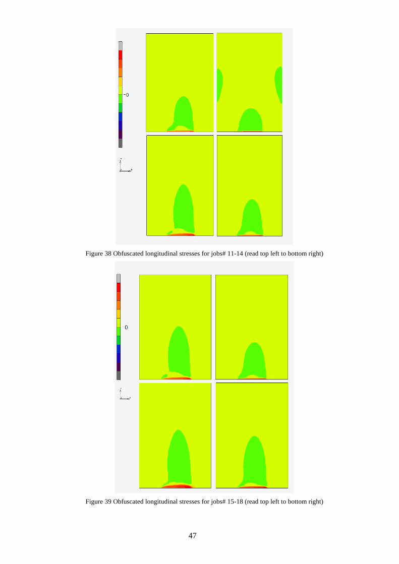
4.2.2 Residual surface stress contour plots
The longitudinal stresses shown in Figure 38 & Figure 39 display a high degree of tensile stress
inside the weld line and a lesser degree of compressive stress over a larger area of the base metal.
The smallest area of tension is found in job# 12 i.e. E3: 83% Power, 50% Spot size, 140% Weld
speed and the largest area in tension is found in job#17 i.e. D2: 117% Power, 150% Spot size, 60%
Weld speed. In terms of the parameter box these two parameters are opposite corners. A similar
trend is suggested for the singular parameters by judging the size of the compressed area.
47
Figure 38 Obfuscated longitudinal stresses for jobs# 11-14 (read top left to bottom right)
Figure 39 Obfuscated longitudinal stresses for jobs# 15-18 (read top left to bottom right)
48
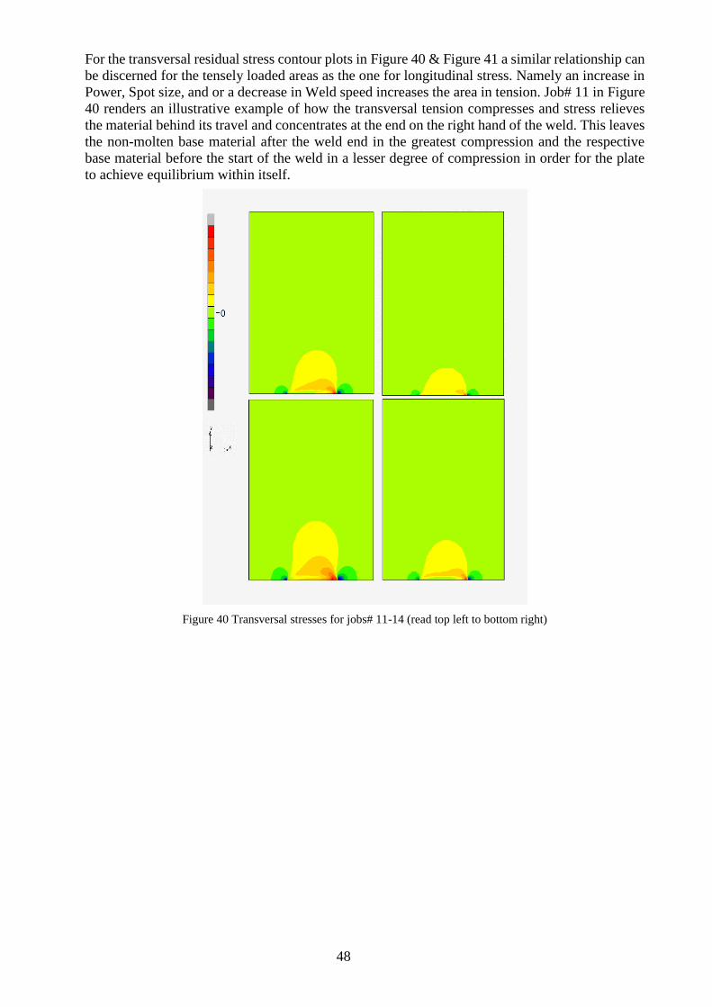
For the transversal residual stress contour plots in Figure 40 & Figure 41 a similar relationship can
be discerned for the tensely loaded areas as the one for longitudinal stress. Namely an increase in
Power, Spot size, and or a decrease in Weld speed increases the area in tension. Job# 11 in Figure
40 renders an illustrative example of how the transversal tension compresses and stress relieves
the material behind its travel and concentrates at the end on the right hand of the weld. This leaves
the non-molten base material after the weld end in the greatest compression and the respective
base material before the start of the weld in a lesser degree of compression in order for the plate
to achieve equilibrium within itself.
Figure 40 Transversal stresses for jobs# 11-14 (read top left to bottom right)
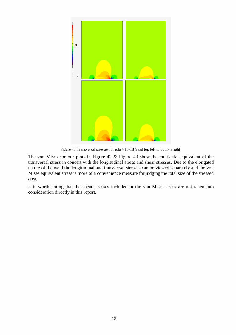
49
Figure 41 Transversal stresses for jobs# 15-18 (read top left to bottom right)
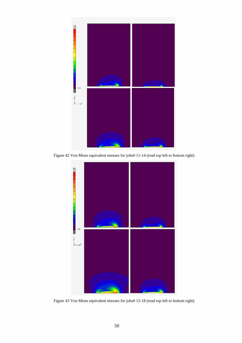
The von Mises contour plots in Figure 42 & Figure 43 show the multiaxial equivalent of the
transversal stress in concert with the longitudinal stress and shear stresses. Due to the elongated
nature of the weld the longitudinal and transversal stresses can be viewed separately and the von
Mises equivalent stress is more of a convenience measure for judging the total size of the stressed
area.
It is worth noting that the shear stresses included in the von Mises stress are not taken into
consideration directly in this report.
50
Figure 42 Von Mises equivalent stresses for jobs# 11-14 (read top left to bottom right)
Figure 43 Von Mises equivalent stresses for jobs# 15-18 (read top left to bottom right)
51
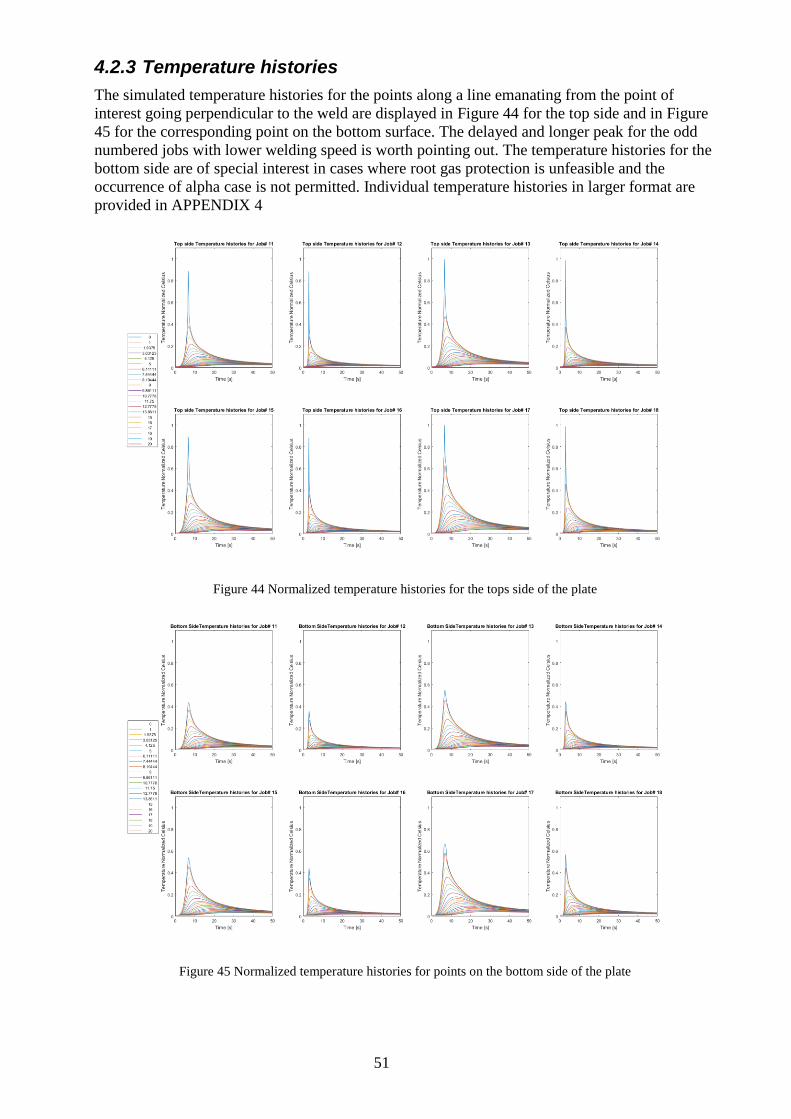
4.2.3 Temperature histories
The simulated temperature histories for the points along a line emanating from the point of
interest going perpendicular to the weld are displayed in Figure 44 for the top side and in Figure
45 for the corresponding point on the bottom surface. The delayed and longer peak for the odd
numbered jobs with lower welding speed is worth pointing out. The temperature histories for the
bottom side are of special interest in cases where root gas protection is unfeasible and the
occurrence of alpha case is not permitted. Individual temperature histories in larger format are
provided in APPENDIX 4
Figure 44 Normalized temperature histories for the tops side of the plate
Figure 45 Normalized temperature histories for points on the bottom side of the plate
52
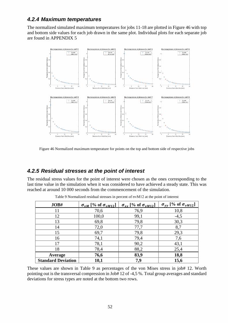
4.2.4 Maximum temperatures
The normalized simulated maximum temperatures for jobs 11-18 are plotted in Figure 46 with top
and bottom side values for each job drawn in the same plot. Individual plots for each separate job
are found in APPENDIX 5
Figure 46 Normalized maximum temperature for points on the top and bottom side of respective jobs
4.2.5 Residual stresses at the point of interest
The residual stress values for the point of interest were chosen as the ones corresponding to the
last time value in the simulation when it was considered to have achieved a steady state. This was
reached at around 10 000 seconds from the commencement of the simulation.
Table 9 Normalized residual stresses in percent of σvM12 at the point of interest
JOB# 𝝈𝒗𝑴 [% of 𝝈𝒗𝑴𝟏𝟐] 𝝈𝒙𝒙 [% of 𝝈𝒗𝑴𝟏𝟐] 𝝈𝒚𝒚 [% of 𝝈𝒗𝑴𝟏𝟐]
11 70,6 76,9 10,8
12 100,0 99,1 -4,5
13 69,8 79,8 30,3
14 72,0 77,7 8,7
15 69,7 79,8 29,3
16 74,1 79,4 7,6
17 78,1 90,2 43,1
18 78,4 88,2 25,4
Average 76,6 83,9 18,8
Standard Deviation 10,1 7,9 15,6
These values are shown in Table 9 as percentages of the von Mises stress in job# 12. Worth
pointing out is the transversal compression in Job# 12 of -4,5 %. Total group averages and standard
deviations for stress types are noted at the bottom two rows.
53
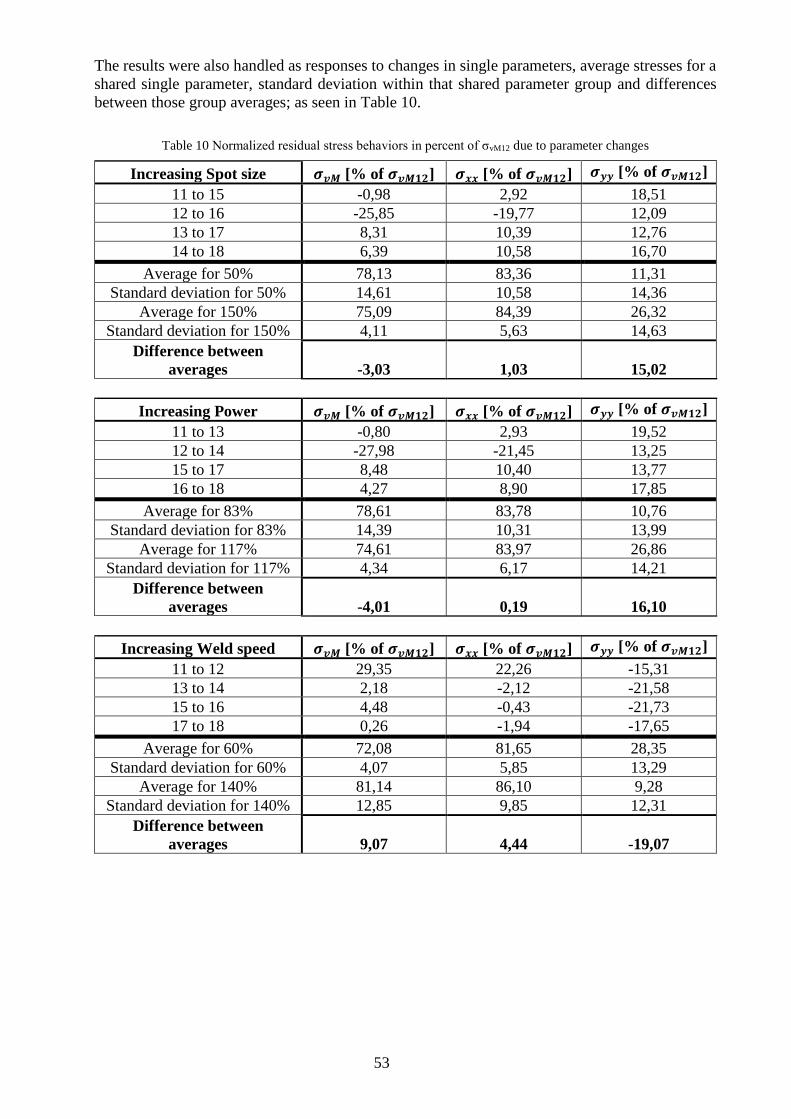
The results were also handled as responses to changes in single parameters, average stresses for a
shared single parameter, standard deviation within that shared parameter group and differences
between those group averages; as seen in Table 10.
Table 10 Normalized residual stress behaviors in percent of σvM12 due to parameter changes
Increasing Spot size 𝝈𝒗𝑴 [% of 𝝈𝒗𝑴𝟏𝟐] 𝝈𝒙𝒙 [% of 𝝈𝒗𝑴𝟏𝟐] 𝝈𝒚𝒚 [% of 𝝈𝒗𝑴𝟏𝟐]
11 to 15 -0,98 2,92 18,51
12 to 16 -25,85 -19,77 12,09
13 to 17 8,31 10,39 12,76
14 to 18 6,39 10,58 16,70
Average for 50% 78,13 83,36 11,31
Standard deviation for 50% 14,61 10,58 14,36
Average for 150% 75,09 84,39 26,32
Standard deviation for 150% 4,11 5,63 14,63
Difference between
averages -3,03 1,03 15,02
Increasing Power 𝝈𝒗𝑴 [% of 𝝈𝒗𝑴𝟏𝟐] 𝝈𝒙𝒙 [% of 𝝈𝒗𝑴𝟏𝟐] 𝝈𝒚𝒚 [% of 𝝈𝒗𝑴𝟏𝟐]
11 to 13 -0,80 2,93 19,52
12 to 14 -27,98 -21,45 13,25
15 to 17 8,48 10,40 13,77
16 to 18 4,27 8,90 17,85
Average for 83% 78,61 83,78 10,76
Standard deviation for 83% 14,39 10,31 13,99
Average for 117% 74,61 83,97 26,86
Standard deviation for 117% 4,34 6,17 14,21
Difference between
averages -4,01 0,19 16,10
Increasing Weld speed 𝝈𝒗𝑴 [% of 𝝈𝒗𝑴𝟏𝟐] 𝝈𝒙𝒙 [% of 𝝈𝒗𝑴𝟏𝟐] 𝝈𝒚𝒚 [% of 𝝈𝒗𝑴𝟏𝟐]
11 to 12 29,35 22,26 -15,31
13 to 14 2,18 -2,12 -21,58
15 to 16 4,48 -0,43 -21,73
17 to 18 0,26 -1,94 -17,65
Average for 60% 72,08 81,65 28,35
Standard deviation for 60% 4,07 5,85 13,29
Average for 140% 81,14 86,10 9,28
Standard deviation for 140% 12,85 9,85 12,31
Difference between
averages 9,07 4,44 -19,07

54
55
5 DISCUSSION AND CONCLUSIONS
This section covers the discussion of the reliability of the results presented in the earlier chapter
in regards of their reliability in generation as well as the reliability of the input data and its
progression from inputs on a welding machine through a physical weld bead, a micrographic
input, and the applicability of the chosen simulation method.
It also tries to answer the research questions stated in the first chapter of this report with respect
to variations between parameter changes of the same type.
5.1 Discussion
5.1.1 Reliability of sample sizes
As there was a limited amount of resources available to this project in terms of machine
availability, laboratory assistance, simulation time and man hours, etc. some limitations had to be
made on sample sizes. Therefore individual results were acquired for measurements, and
simulations which were seen as representative for those parameter sets without any further
sampling within that parameter set.
5.1.2 Reliability of physical data outputs
As noted in chapter 2, Ti64 is highly reflective material which hampers accurate measurements of
weld geometries. To address this possible inaccuracy, either a repeated set of measurements would
need to be taken for each weld parameter or another method would need to be devised for
measuring the weld geometry. This was deemed to be too time and resource consuming why the
measured geometries were taken as exact values for simulation input.
The temperature sensor had a refresh frequency estimated at about 1Hz, which was one of the
reasons for the repeated measurements at 1mm yielding a standard deviation of 2,6 Celsius. This
was deemed acceptable but a continuous measurement connected to a continuous plotter would
yield a physical measurement of the temperature history.
5.1.3 Reliability of physical data inputs
As a highly reflective and somewhat exotic material the thermal coupling coefficient of the laser
beam into the Ti64 BM might not be certain for this equipment as it is traditionally applied in
welding ferritic materials. Thus a calibration study conducted by an operator used to laser welding
Ti64 is desired; this in order to establish a clear image of the equipment’s laser spot and its coupling
into this material.
Thermally, Ti64 is a relatively isolating material with about half the thermal conductivity of steel.
This in conjunction with the somewhat isolating fixturing and low energy nature of the weld might
result in the cooling effects of the shielding gas playing a larger role than it does in more energy
intensive welds where more simulation experience is accumulated at GKN.
These two factors are believed to be partly responsible for the lower nature of the measured
maximum temperatures.
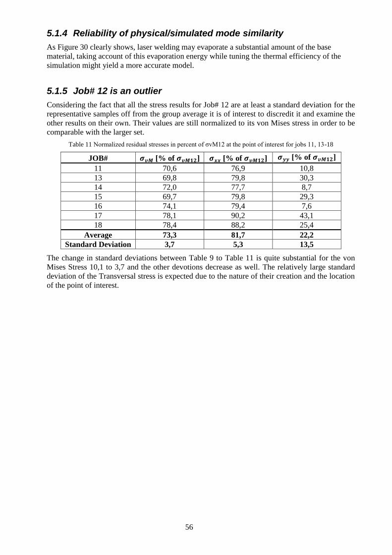
56
5.1.4 Reliability of physical/simulated mode similarity
As Figure 30 clearly shows, laser welding may evaporate a substantial amount of the base
material, taking account of this evaporation energy while tuning the thermal efficiency of the
simulation might yield a more accurate model.
5.1.5 Job# 12 is an outlier
Considering the fact that all the stress results for Job# 12 are at least a standard deviation for the
representative samples off from the group average it is of interest to discredit it and examine the
other results on their own. Their values are still normalized to its von Mises stress in order to be
comparable with the larger set.
Table 11 Normalized residual stresses in percent of σvM12 at the point of interest for jobs 11, 13-18
JOB# 𝝈𝒗𝑴 [% of 𝝈𝒗𝑴𝟏𝟐] 𝝈𝒙𝒙 [% of 𝝈𝒗𝑴𝟏𝟐] 𝝈𝒚𝒚 [% of 𝝈𝒗𝑴𝟏𝟐]
11 70,6 76,9 10,8
13 69,8 79,8 30,3
14 72,0 77,7 8,7
15 69,7 79,8 29,3
16 74,1 79,4 7,6
17 78,1 90,2 43,1
18 78,4 88,2 25,4
Average 73,3 81,7 22,2
Standard Deviation 3,7 5,3 13,5
The change in standard deviations between Table 9 to Table 11 is quite substantial for the von
Mises Stress 10,1 to 3,7 and the other devotions decrease as well. The relatively large standard
deviation of the Transversal stress is expected due to the nature of their creation and the location
of the point of interest.
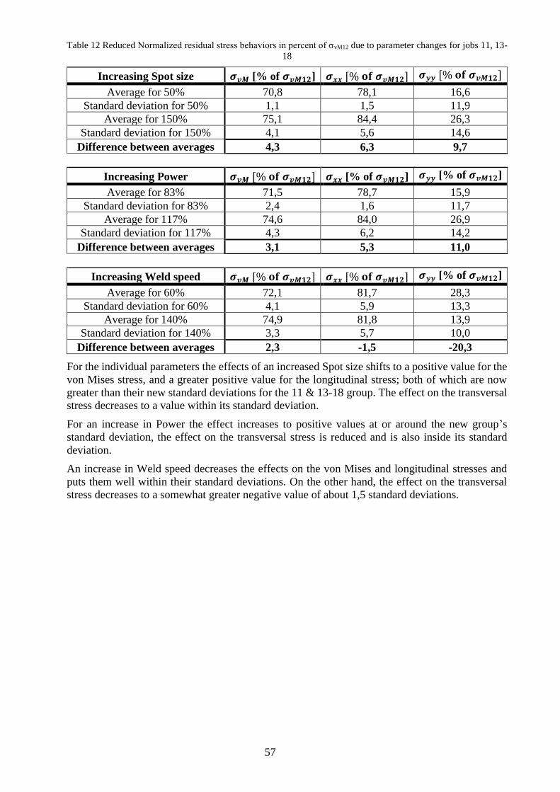
57
Table 12 Reduced Normalized residual stress behaviors in percent of σvM12 due to parameter changes for jobs 11, 13-
18
Increasing Spot size 𝝈𝒗𝑴 [% of 𝝈𝒗𝑴𝟏𝟐] 𝝈𝒙𝒙 [% 𝐨𝐟 𝝈𝒗𝑴𝟏𝟐] 𝝈𝒚𝒚 [% 𝐨𝐟 𝝈𝒗𝑴𝟏𝟐]
Average for 50% 70,8 78,1 16,6
Standard deviation for 50% 1,1 1,5 11,9
Average for 150% 75,1 84,4 26,3
Standard deviation for 150% 4,1 5,6 14,6
Difference between averages 4,3 6,3 9,7
Increasing Power 𝝈𝒗𝑴 [% 𝐨𝐟 𝝈𝒗𝑴𝟏𝟐] 𝝈𝒙𝒙 [% of 𝝈𝒗𝑴𝟏𝟐] 𝝈𝒚𝒚 [% of 𝝈𝒗𝑴𝟏𝟐]
Average for 83% 71,5 78,7 15,9
Standard deviation for 83% 2,4 1,6 11,7
Average for 117% 74,6 84,0 26,9
Standard deviation for 117% 4,3 6,2 14,2
Difference between averages 3,1 5,3 11,0
Increasing Weld speed 𝝈𝒗𝑴 [% 𝐨𝐟 𝝈𝒗𝑴𝟏𝟐] 𝝈𝒙𝒙 [% 𝐨𝐟 𝝈𝒗𝑴𝟏𝟐] 𝝈𝒚𝒚 [% of 𝝈𝒗𝑴𝟏𝟐]
Average for 60% 72,1 81,7 28,3
Standard deviation for 60% 4,1 5,9 13,3
Average for 140% 74,9 81,8 13,9
Standard deviation for 140% 3,3 5,7 10,0
Difference between averages 2,3 -1,5 -20,3
For the individual parameters the effects of an increased Spot size shifts to a positive value for the
von Mises stress, and a greater positive value for the longitudinal stress; both of which are now
greater than their new standard deviations for the 11 & 13-18 group. The effect on the transversal
stress decreases to a value within its standard deviation.
For an increase in Power the effect increases to positive values at or around the new group’s
standard deviation, the effect on the transversal stress is reduced and is also inside its standard
deviation.
An increase in Weld speed decreases the effects on the von Mises and longitudinal stresses and
puts them well within their standard deviations. On the other hand, the effect on the transversal
stress decreases to a somewhat greater negative value of about 1,5 standard deviations.
58
5.2 Conclusions
5.2.1 Individual Parameter Responses
An increase in Spot size or Power did not yield any parameter responses greater than one standard
deviation on the von Mises or longitudinal stresses. A weak trend towards their increase leading
to an increase of transversal stress is noted.
An increase in Weld speed shows an increase in von Mises stress that is below the standard
deviation, a sign shifting effect on longitudinal stress that is well below the standard deviation and
a statistically significant decrease in transversal residual stresses.
5.2.2 Synergetic Parameter Responses
It was found that an increase in Power and a decrease in Weld speed together with an increase in
Spot size, colloquially speaking a hotter and wider weld, will have an increased area that is
subjected to residual stresses.
It is the conclusion of this report that the residual stresses resulting from repair welds within its
parameter box cannot be practically reduced to a negligible value, their extent in the base material
may on the other hand be minimized and their shape described with the help of its findings.
59
6 RECOMMENDATIONS AND FUTURE WORK
6.1 Recommendations
It is the recommendation of the author that future studies in this area should be started with, and
structured after the simulation tools’ and expertise’s strengths and weaknesses. While still
regarding the practical welding implications in mind but with them in second hand to the
simulation implications.
The author stresses the importance of testing the outlying parameters in a response surface set up
first, this in order to avoid “boxing oneself in against a wall” with conducted experiments as a sunk
cost and desired future experiments being unattainable for some previously unknown reason.
6.2 Future work
The author would recommend a master’s student with an interest in FEM-simulations & heat
transfer as well as at least a cursory interest in welding to contact GKN in inquiry of a possible
master’s thesis regarding the refinement and efficiency of heat transfer models and welding
simulations of low energy laser welding.
The author would recommend a master’s student with an interest in fluid dynamics and welding
to contact GKN in inquiry of a possible master’s thesis regarding the effects of weld parameters
and their synergies on the establishment and maintenance of a welding keyhole.

60
61
7 REFERENCES
Olabi A. G. et al., ”Application of Response Surface Methodology in Describing the Residual
Stress Distribution in CO2 Laser Welding of AISI304”, Strain, Vol. 43, 2007, 37-46
Turner R. P. et al., ”An Integrated Modeling Approach for Predicting Process Maps of Residual
Stress and Distortion in a Laser Weld: A Combined CFD–FE Methodology”, METALLURGICAL
AND MATERIALS TRANSACTIONS, Vol. 47B, 2016, pp 2954-2962
Colegrove P. et al., ”Welding process impact on residual stress and distortion”, Science and
Technology of Welding and Joining, Vol. 14, 2009, pp 717-725
AZO Materials, ” Titanium Alloys - Ti6Al4V Grade 5”,
https://www.azom.com/article.aspx?ArticleID=1547, accessed 2018-06-18.
SSAB, ”Strenx 900”, https://www.ssab.com/Products/Brands/Strenx/Products/Strenx-900,
accessed 2018-06-18.
Wikipedia, ”Titanium”, https://en.wikipedia.org/wiki/Titanium, accessed 2018-16-18.
Wikipedia, ”Iron”, https://en.wikipedia.org/wiki/Iron, accessed 2018-06-18.
Performance Titanium Group, “ASTM B348 6AL-4V Grade 5”,
https://performancetitanium.com/astm-b348-6al-4v-grade-5/, accessed 2018-06-18
Radaj D., “Heat Effects of Welding”, Springer-Verlag, Berlin, 1992.
Lütjering G. and Williams J.C., “Titanium”, Springer, Berlin, 2007
Katayama S. “Handbook of laser welding technologies”, Woodhead Publishing, Philadelphia,
2013
Alphalaser, “ ALFlak SELF-PROPELLED, ROBUST, PROGRAMMABLE”,
https://alphalaser.de/fileadmin/user_upload/Datenblaetter/Datenblatt_ALFlak_2015_Eng.pdf,
accessed 2018-05-04, 2015.
Rossini N.S. Dassisti M., Benyounis K.Y. and Olabi A.G., ”Methods of measuring residual
stresses in components”, Materials and Design, Vol. 35, 2012, pp 572-588
Hosseinzadeh F., Kowal J., Bouchard P.J., “Towards good practice guidelines for the contour
method of residual stress measurement”, The Journal of Engineering, Vol 2014 issue 8, pp 453-
468.
Revie W.R., “CORROSION AND CORROSION CONTROL”, John Wiley & Sons, Hoboken, 2008.
Evans R.W., Hull R.J.and Wilshire B., “THE EFFECTS OF ALPHA-CASE FORMATION ON
THE CREEP FRACTURE PROPERTIES OF THE HIGH-TEMPERATURE TITANIUM ALLOY
IMI834”, Journal of Materials Processing Technology, Vol. 56, 1996, pp 492-501

62
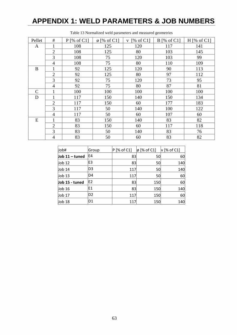
63
APPENDIX 1: WELD PARAMETERS & JOB NUMBERS
Table 13 Normalized weld parameters and measured geometries
Pellet # P [% of C1] ø [% of C1] v [% of C1] B [% of C1] H [% of C1]
A 1 108 125 120 117 141
2 108 125 80 103 145
3 108 75 120 103 99
4 108 75 80 110 109
B 1 92 125 120 90 113
2 92 125 80 97 112
3 92 75 120 73 95
4 92 75 80 87 81
C 1 100 100 100 100 100
D 1 117 150 140 150 134
2 117 150 60 177 183
3 117 50 140 100 122
4 117 50 60 107 60
E 1 83 150 140 83 82
2 83 150 60 117 118
3 83 50 140 83 76
4 83 50 60 83 82
Job# Group P [% of C1] ø [% of C1] v [% of C1]
Job 11 – tuned E4 83 50 60
Job 12 E3 83 50 140
Job 14 D3 117 50 140
Job 13 D4 117 50 60
Job 15 - tuned E2 83 150 60
Job 16 E1 83 150 140
Job 17 D2 117 150 60
Job 18 D1 117 150 140

64
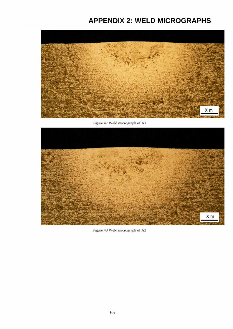
65
APPENDIX 2: WELD MICROGRAPHS
Figure 47 Weld micrograph of A1
Figure 48 Weld micrograph of A2
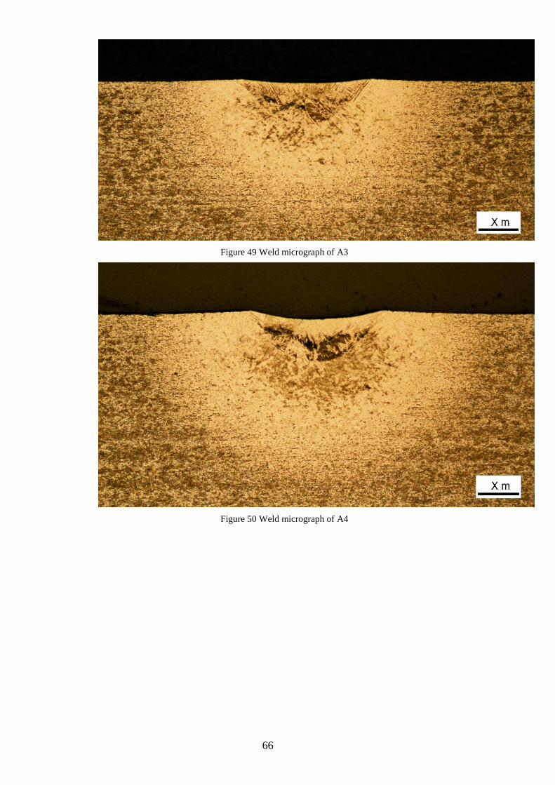
66
Figure 49 Weld micrograph of A3
Figure 50 Weld micrograph of A4
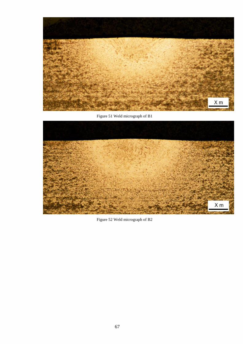
67
Figure 51 Weld micrograph of B1
Figure 52 Weld micrograph of B2
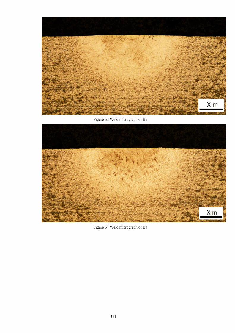
68
Figure 53 Weld micrograph of B3
Figure 54 Weld micrograph of B4
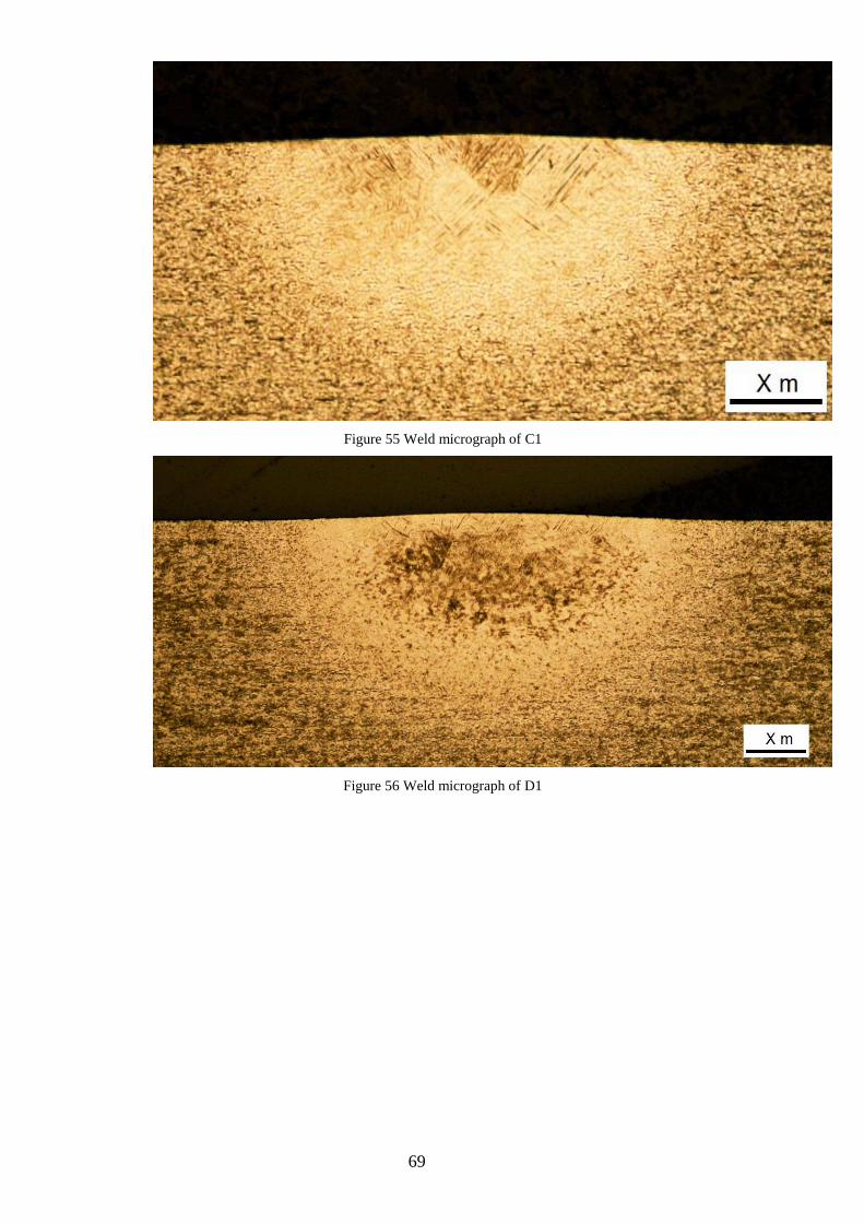
69
Figure 55 Weld micrograph of C1
Figure 56 Weld micrograph of D1
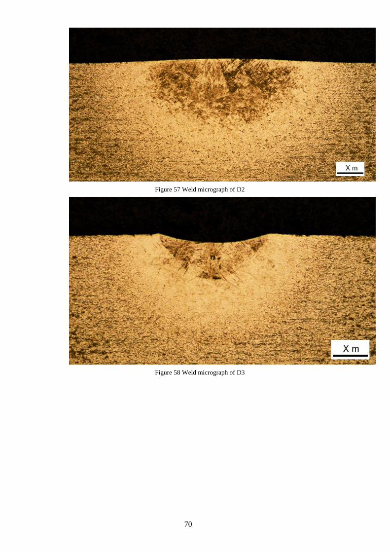
70
Figure 57 Weld micrograph of D2
Figure 58 Weld micrograph of D3
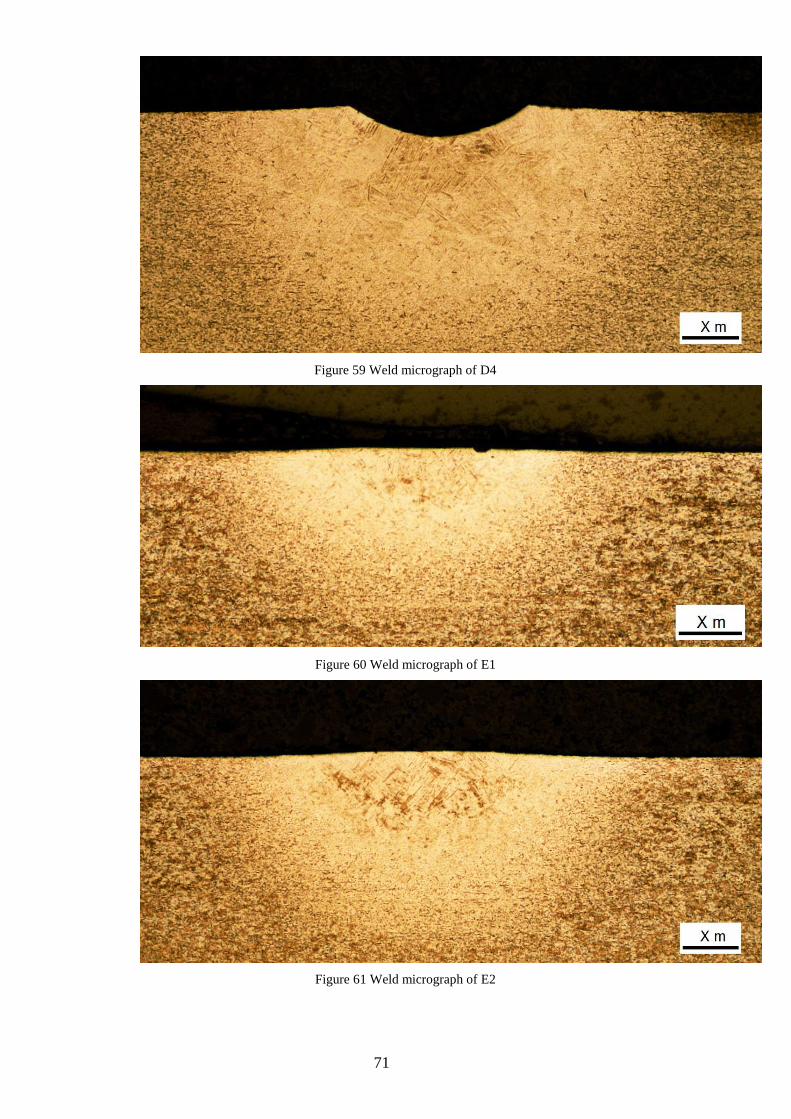
71
Figure 59 Weld micrograph of D4
Figure 60 Weld micrograph of E1
Figure 61 Weld micrograph of E2
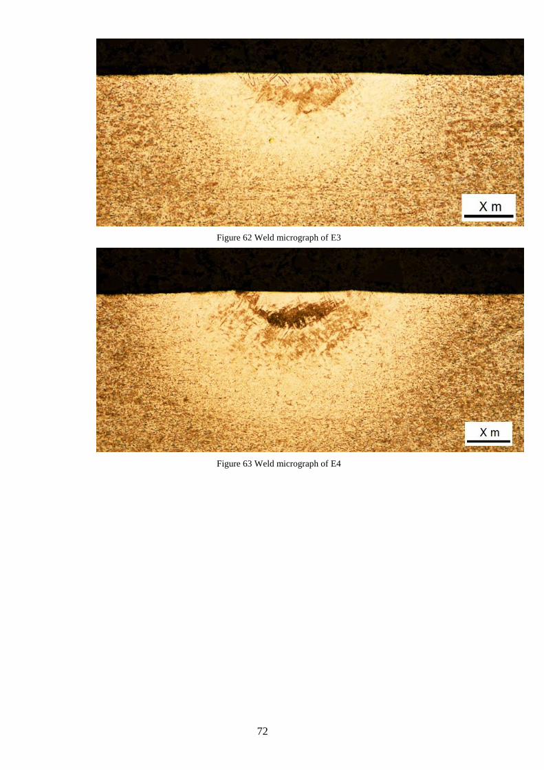
72
Figure 62 Weld micrograph of E3
Figure 63 Weld micrograph of E4
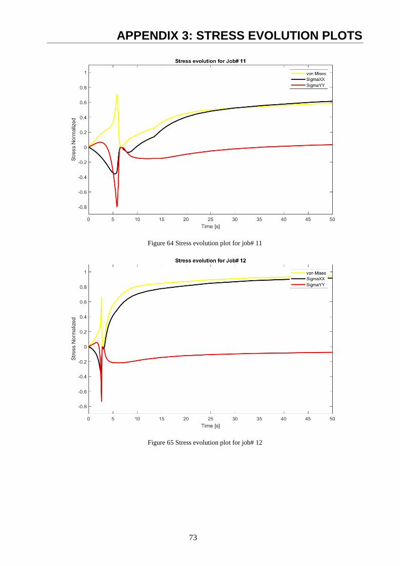
73
APPENDIX 3: STRESS EVOLUTION PLOTS
Figure 64 Stress evolution plot for job# 11
Figure 65 Stress evolution plot for job# 12
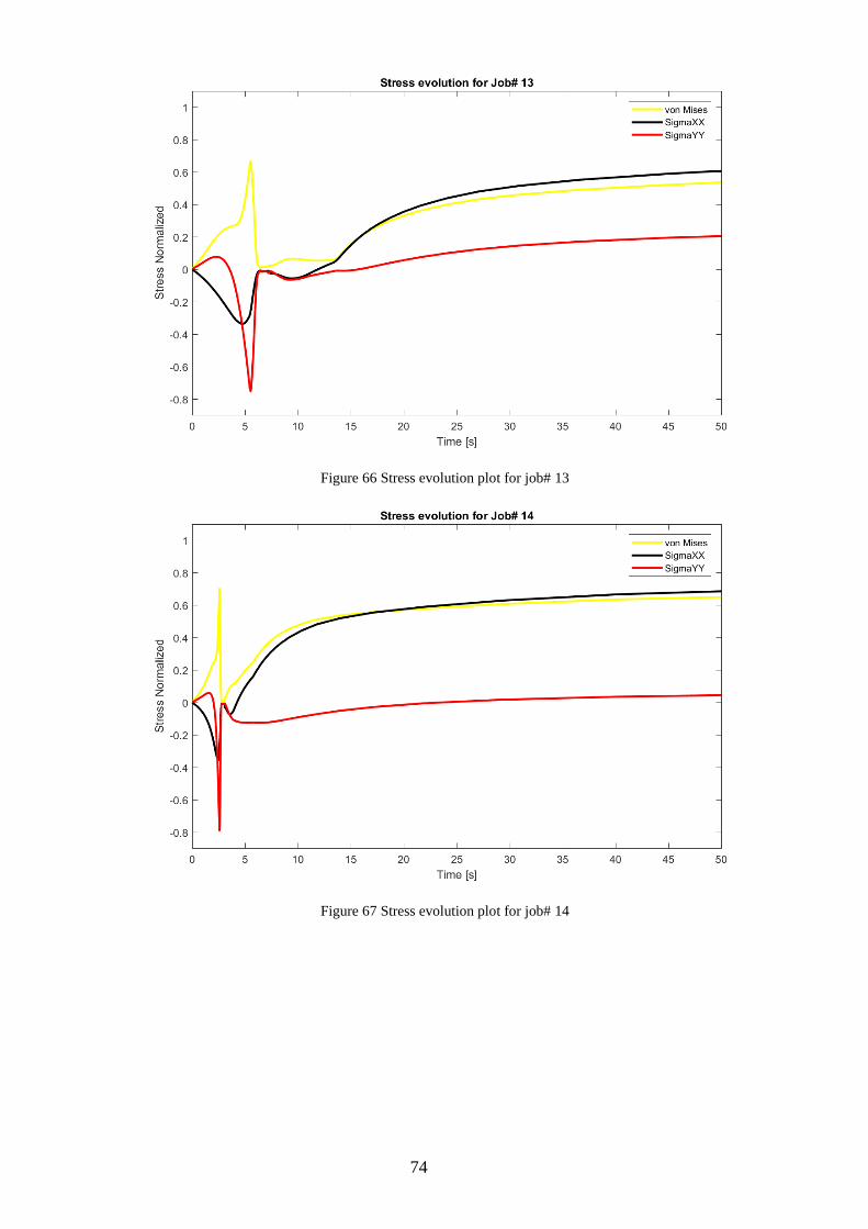
74
Figure 66 Stress evolution plot for job# 13
Figure 67 Stress evolution plot for job# 14
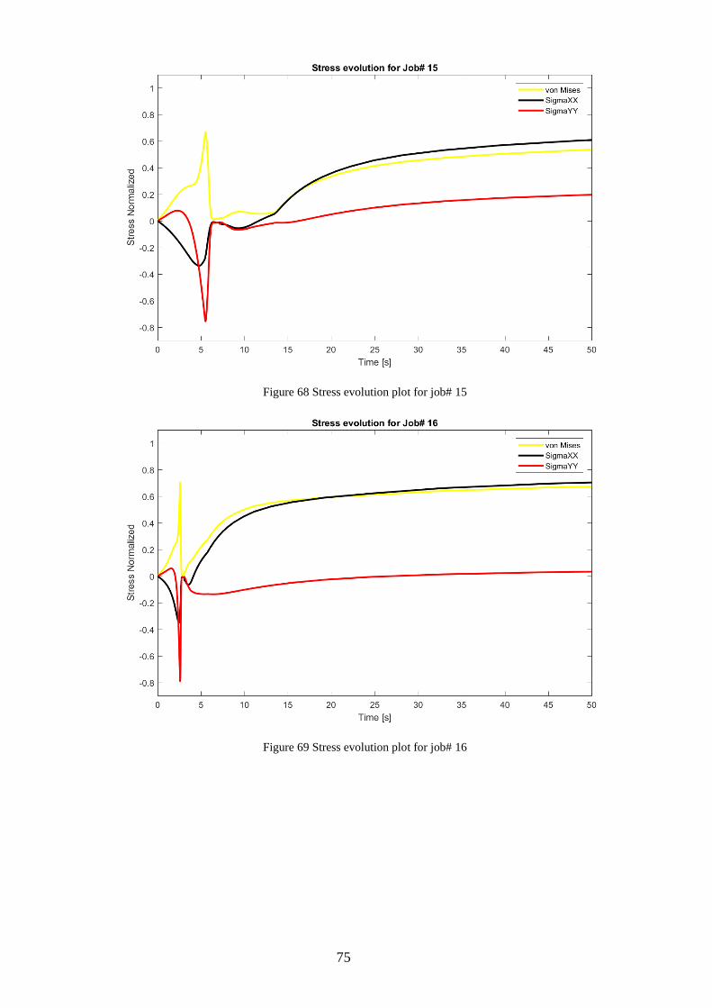
75
Figure 68 Stress evolution plot for job# 15
Figure 69 Stress evolution plot for job# 16
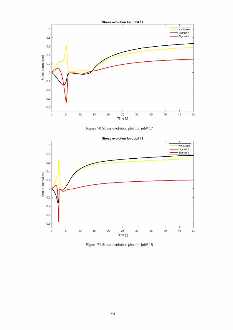
76
Figure 70 Stress evolution plot for job# 17
Figure 71 Stress evolution plot for job# 18
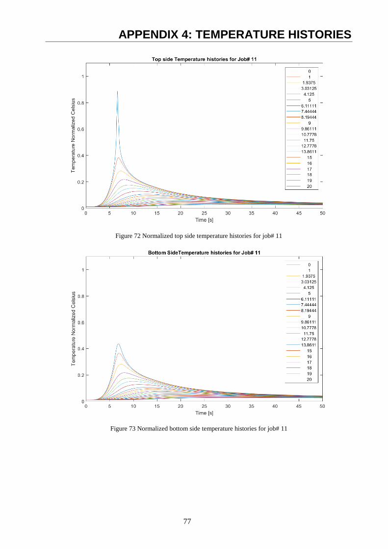
77
APPENDIX 4: TEMPERATURE HISTORIES
Figure 72 Normalized top side temperature histories for job# 11
Figure 73 Normalized bottom side temperature histories for job# 11
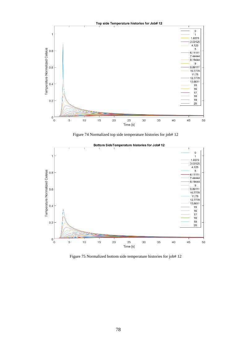
78
Figure 74 Normalized top side temperature histories for job# 12
Figure 75 Normalized bottom side temperature histories for job# 12
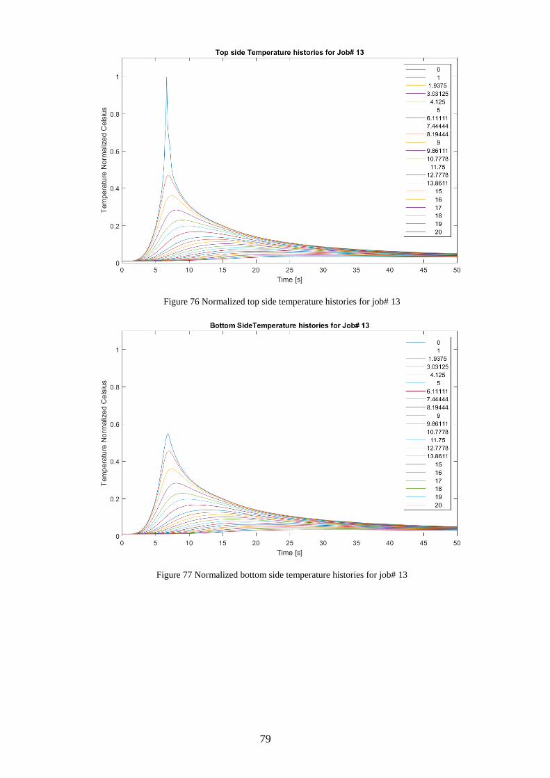
79
Figure 76 Normalized top side temperature histories for job# 13
Figure 77 Normalized bottom side temperature histories for job# 13
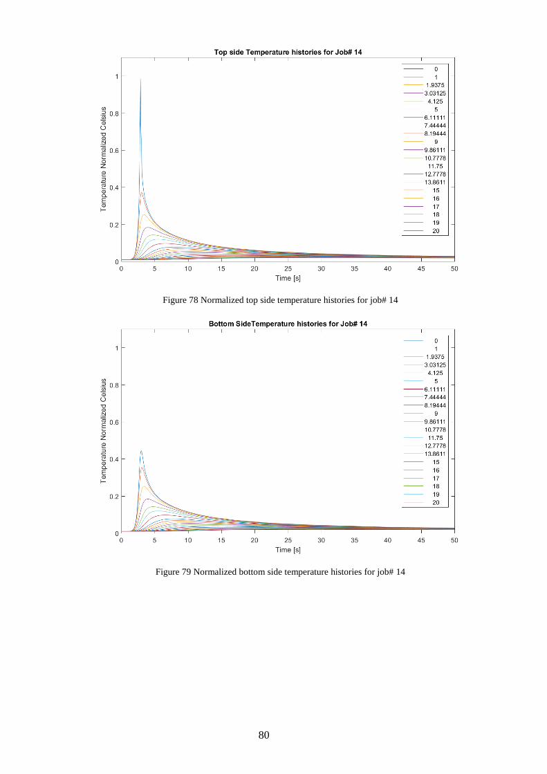
80
Figure 78 Normalized top side temperature histories for job# 14
Figure 79 Normalized bottom side temperature histories for job# 14
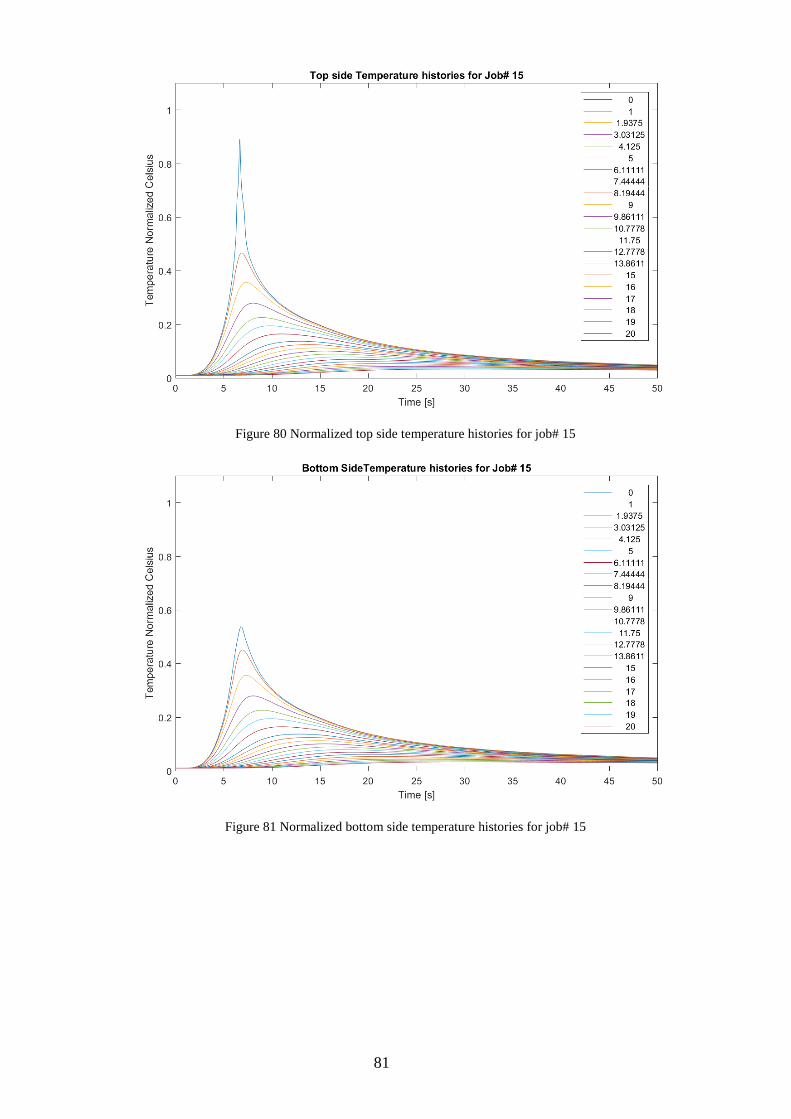
81
Figure 80 Normalized top side temperature histories for job# 15
Figure 81 Normalized bottom side temperature histories for job# 15
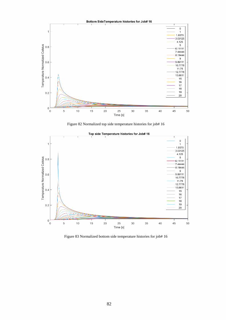
82
Figure 82 Normalized top side temperature histories for job# 16
Figure 83 Normalized bottom side temperature histories for job# 16
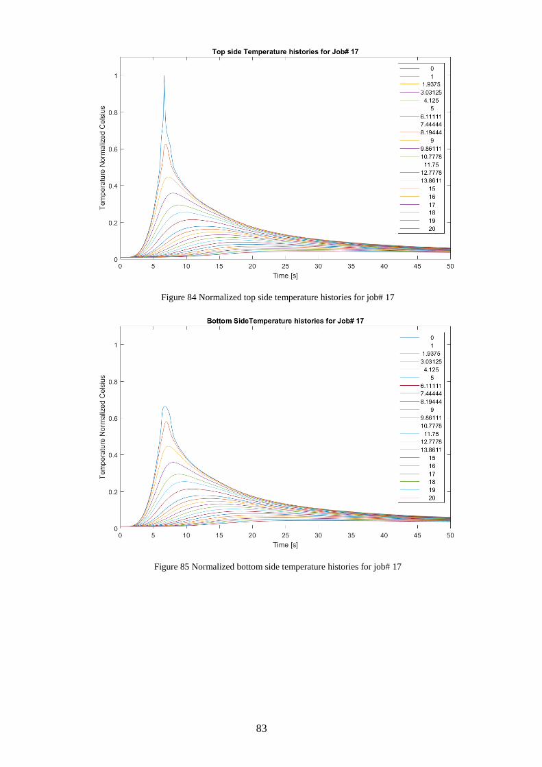
83
Figure 84 Normalized top side temperature histories for job# 17
Figure 85 Normalized bottom side temperature histories for job# 17
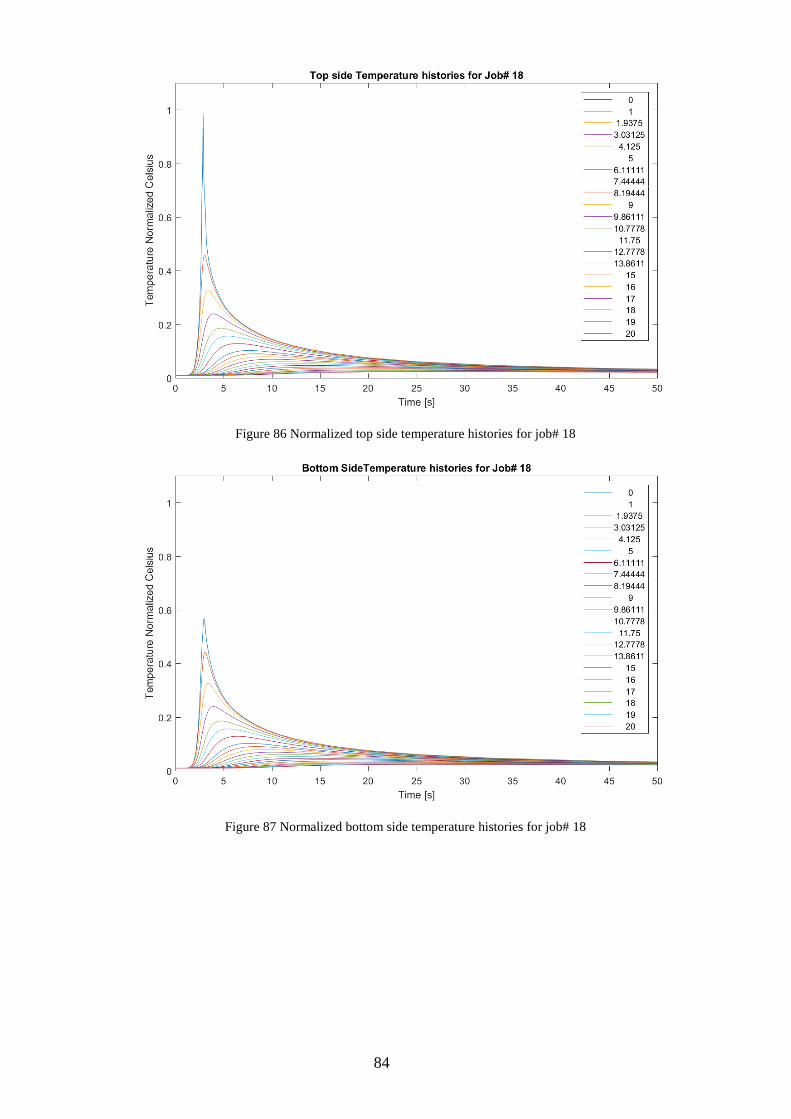
84
Figure 86 Normalized top side temperature histories for job# 18
Figure 87 Normalized bottom side temperature histories for job# 18
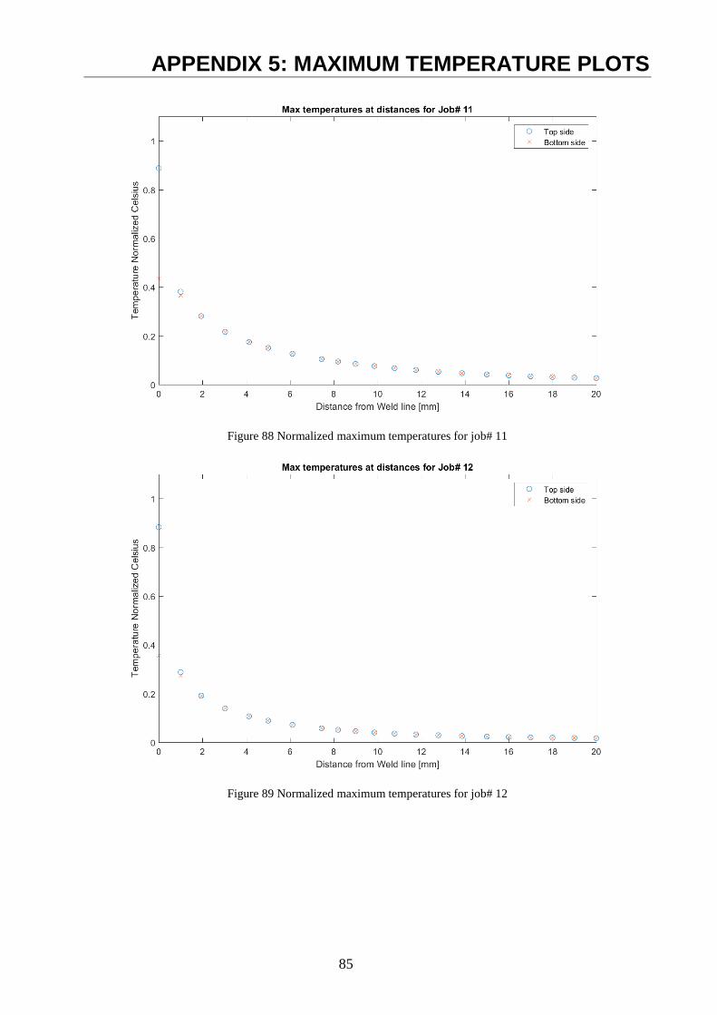
85
APPENDIX 5: MAXIMUM TEMPERATURE PLOTS
Figure 88 Normalized maximum temperatures for job# 11
Figure 89 Normalized maximum temperatures for job# 12

86
Figure 90 Normalized maximum temperatures for job# 13
Figure 91 Normalized maximum temperatures for job# 14

87
Figure 92 Normalized maximum temperatures for job# 15
Figure 93 Normalized maximum temperatures for job# 16
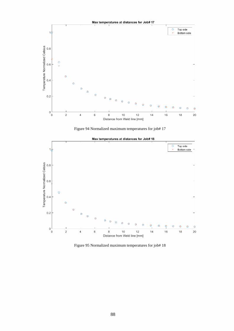
88
Figure 94 Normalized maximum temperatures for job# 17
Figure 95 Normalized maximum temperatures for job# 18
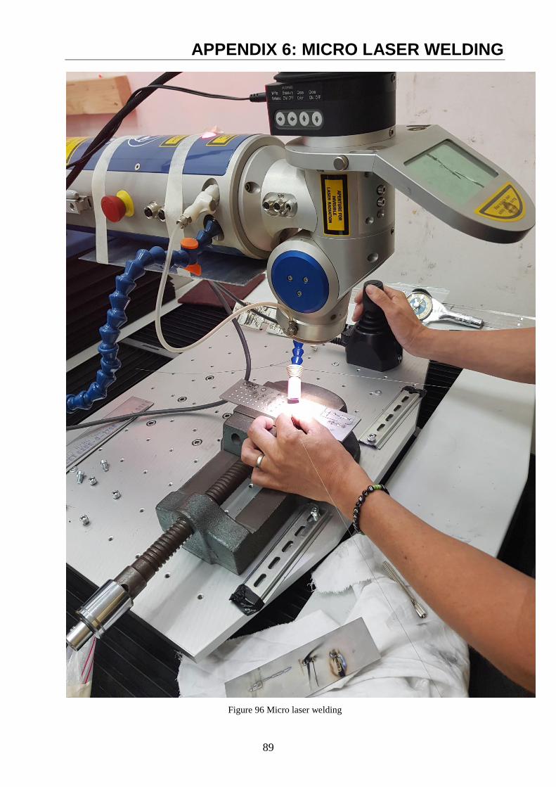
89
APPENDIX 6: MICRO LASER WELDING
Figure 96 Micro laser welding

90
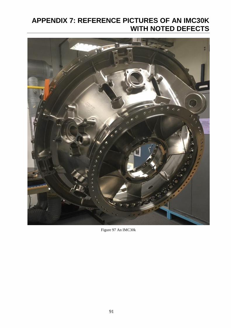
91
APPENDIX 7: REFERENCE PICTURES OF AN IMC30K WITH NOTED DEFECTS
Figure 97 An IMC30k
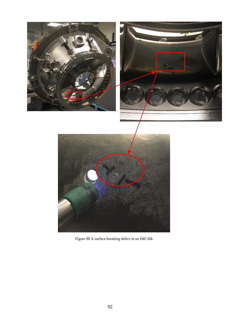
92
Figure 98 A surface breaking defect in an IMC30k
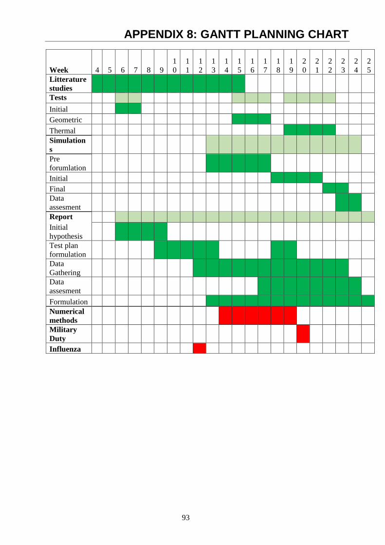
93
APPENDIX 8: GANTT PLANNING CHART
Week 4 5 6 7 8 9
1
0
1
1
1
2
1
3
1
4
1
5
1
6
1
7
1
8
1
9
2
0
2
1
2
2
2
3
2
4
2
5
Litterature
studies
Tests
Initial
Geometric
Thermal
Simulation
s
Pre
forumlation
Initial
Final
Data
assesment
Report
Initial
hypothesis
Test plan
formulation
Data
Gathering
Data
assesment
Formulation
Numerical
methods
Military
Duty
Influenza


![INSTRUKTIONSHÄFTE - Home | CASIO · Använd sifferknapparna och knapparna [–] och [+] för att ändra inställningar för parametrarna som visas på skärmens övre vänstra del](https://img.pdfslide.net/doc/110x75/5f28f7685f16f5693274a9de/instruktionshfte-home-casio-anvnd-sifferknapparna-och-knapparna-a-och.jpg)