A AECL EACL

CA0000130

AECL-11571, COG-96-157-1

Biotite Dissolution and Oxygen Consumption inAqueous Media at 100°C

Dissolution de la biotite et consommation d'oxygenedans un support aqueux a 100 °C

Peter Taylor, Derrek G. Owen

April 1997avril

A AECL EACL

BIOTITE DISSOLUTION AND OXYGEN CONSUMPTION

IN AQUEOUS MEDIA AT 100°C

by

Peter Taylor and Derrek G. Owen

Whiteshell LaboratoriesPinawa, Manitoba ROE 1L0

1997

AECL-11571COG-96-157-1

A AECL EACL

BIOTITE DISSOLUTION AND OXYGEN CONSUMPTION

IN AQUEOUS MEDIA AT IOO°C

by

Peter Taylor and Derrek G. Owen

ABSTRACT

The ability of biotite to consume dissolved oxygen, and hence restore reducing conditions in anuclear fuel waste vault after closure, has been assessed experimentally. Oxygen consumptionhas been measured directly, and also deduced from experimental biotite dissolution rates.Results from the dissolution experiments on granitic biotite from the Lac du Bonnet region,Manitoba indicate that the biotite component of granite backfill should consume entrainedoxygen in about 50 years at 100°C. Direct measurements of oxygen consumption by commercialbiotite specimens originating from Bancroft, Ontario were reasonably consistent with thisfinding. Magnetite is significantly more effective than biotite at oxygen consumption, perhapstwo orders of magnitude faster at 100°C.

Whiteshell LaboratoriesPinawa, Manitoba ROE 1L0

1997

AECL-11571COG-96-157-1

AECL EACL

DISSOLUTION DE LA BIOTITE ET CONSOMMATION D'OXYGENE

DANS UN SUPPORT AQUEUX A 100 °C

par

Peter Taylor et Derrek G. Owen

RESUME

On a evalue de facon experimentale la capacite de la biotite a consumer l'oxygene dissous et, parconsequent, a retablir les conditions reductrices dans une enceinte de dechets de combustiblenucleaire apres sa fermeture. La consommation d'oxygene a ete mesuree directement et pardeduction a partir des vitesses de dissolution experimentale de la biotite. Les resultats desexperiences sur la dissolution de la biotite granitique dans la region de Lac du Bonnet, auManitoba, indiquent que la composante de biotite du remblai granitique devrait consumerl'oxygene entraine au bout de 50 ans a une temperature de 100 °C. Les mesures directes de laconsommation d'oxygene par des specimens de biotite commerciale provenant de Bancroft, enOntario, ont produit des resultats semblables. La magnetite est considerablement plus efficaceque la biotite pour ce qui est de la consommation d'oxygene, peut-etre de deux ordres degrandeur plus rapide a 100 °C.

Laboratoires WhiteshellPinawa (Manitoba) ROE 1L0

1997

AECL-11571COG-96-157-1

CONTENTS

Page

1. INTRODUCTION 1

2. BIOTITE DISSOLUTION ]

2.1 BIOTITE CRYSTAL CHEMISTRY I2.2 MINERAL DISSOLUTION GENERALITIES 32.3 THE STOICHIOMETRY OF DISSOLUTION AND ALTERATION 42.4 THE LINK BETWEEN POTASSIUM RELEASE AND IRON REDOX

CHEMISTRY 72.5 SUMMARY OF DISSOLUTION EXPERIMENTS ON BIOTITE 8

3 NEW EXPERIMENTS ON BIOTITE DISSOLUTION 9

3.1 DESIGN OF CURRENT EXPERIMENTS 103.2 RESULTS AND CALCULATIONS 11

3.2.1 Potassium Release 1 ]3.2.2 Magnesium Release 123.2.3 Silicon Release 123.2.4 Comparison of fractional release of magnesium and silicon 133.2.5 The vexatious question of surface area 14

3.3 DISCUSSION 15

4 DIRECT MEASUREMENT OF OXYGEN CONSUMPTION 16

4.1 BACKGROUND AND EARLY DIFFICULTIES 164.2 EXPERIMENTAL 174.3 RESULTS 17

4.4 DISCUSSION 18

5 CONCLUSIONS AND RECOMMENDATIONS 19

ACKNOWLEDGEMENTS 20

REFERENCES 20

TABLES 23

FIGURES 40

1. INTRODUCTION

The Canadian Nuclear Fuel Waste Management Program is based on the concept of directdisposal of used UO2 fuel bundles in corrosion-resistant containers in an engineered vault withina granite pluton on the Canadian Shield (Hancox and Nuttall 1991, Johnson et al. 1994). Afterthe vault is sealed, it is desirable for any oxygen entrained in the backfill to be removed rapidlyand for reducing conditions to be restored. This will minimize corrosion of container materialsand subsequent oxidative dissolution of UO2. In particular, it would eliminate the oxygen-drivencrevice corrosion of titanium-based container materials (Shoesmith et al. 1995).

Iron-containing minerals, such as magnetite and biotite, are expected to contribute to oxygenremoval in the vault. Scoping calculations based on reported weathering rates indicated that thebiotite component of backfill should remove entrained oxygen within 320 years at 25°C or 8years at 80°C (Johnson et al. 1994). Experiments with synthetic magnetite powders haverevealed substantial conversion to hematite within a few weeks at 100°C, indicating thatmagnetite should also be an effective oxygen scavenger (Taylor and Owen 1993).

We are conducting experiments to evaluate the ability of biotite and magnetite to remove oxygenfrom aqueous solution. Two approaches are being taken in these experiments. One is to measureoxygen removal directly. The other is to measure biotite dissolution rates and hence try to inferthe availability of Fe2+ for both oxygen removal and subsequent establishment of reducingconditions. This report presents recent findings from both types of experiment. Somepreliminary results from biotite dissolution/alteration experiments have been reported previously(Taylor and Owen 1995).

2. BIOTITE DISSOLUTION

2.1 BIOTITE CRYSTAL CHEMISTRY

Biotite is a complex potassium magnesium iron aluminosilicate belonging to the trioctahedralmica group of minerals, with a range of nominal compositions represented by the formula:

K(Mgo.6-i.8Fe"24-l2)Si3A1010(OH,F)2 . (1)

In some publications on biotite, this formula is doubled; all the formulae used in the presentreport have been converted to the smaller formula unit, which is also used to express "moles ofbiotite" in dissolution rates. In converting empirical analyses to structural formulae, cationconcentrations are normalized to a total anionic charge of 22, i.e., Oio(OH,F)2. The cations inthis formula fall into three major groups:

(a) Exchangeable interlayer cations, primarily K+ with minor quantities of Na+ and Ca2+;(b) Octahedrally coordinated species in the centre of the aluminosilicate "sandwich", primarilyMg2+and Fe2+, with some Al1+, Fe3+, Mn2+, Ti4+ and other minor constituents;(c) Tetrahedrally coordinated species forming the outer layers of the sandwich sheet, primarilyAl3* and Si4+, with some Fe3+.

Here, all species are given an ionic notation for ease of charge-balance calculations; it isrecognized that Si, in particular, has a large covalent contribution to its bonding. The following

discussion is intended to give some idea of the variability of biotite composition, but is far fromcomprehensive. It focuses on the compositions of biotite investigated in previous dissolution oralteration studies. For a more detailed discussion of biotite compositions, see Bailey (1984).

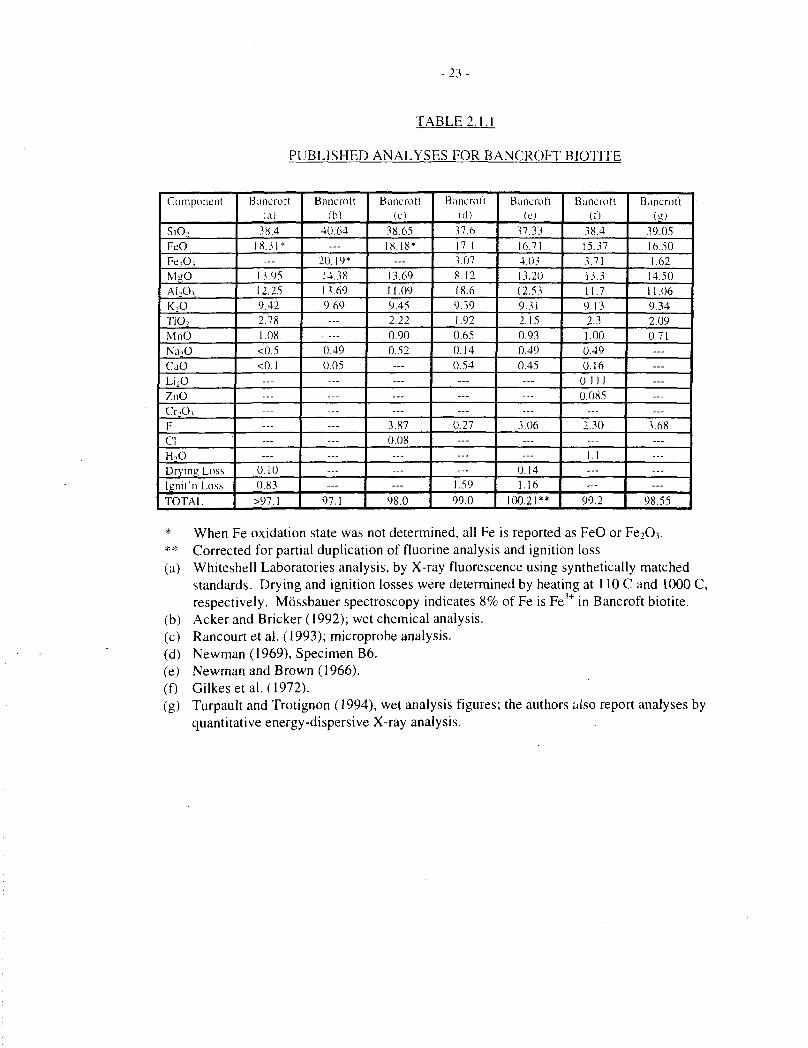
One source of mineralogically pure, highly crystalline biotite is Bancroft, Ontario. Severalpublished laboratory dissolution studies have been based on this material (Acker and Bricker1992, Gilkes et al. 1973, Newman and Brown 1966, Taylor and Owen 1995, Turpault andTrotignon 1994). Published analyses vary somewhat, partly because they are sometimesincomplete and partly (presumably) because of inter-sample variation. Calculated structuralformulae vary correspondingly. A formula based on one of the most recent and completeanalyses (Turpault and Trotignon 1994), but omitting minor quantities of Na, is:

Koy2(MgI66Fe"i.o6Fe"Io.o')4Tio.i2Mnoo46)(SiLooAl|.ooOio(OH)MoFo.lx)) . (2)

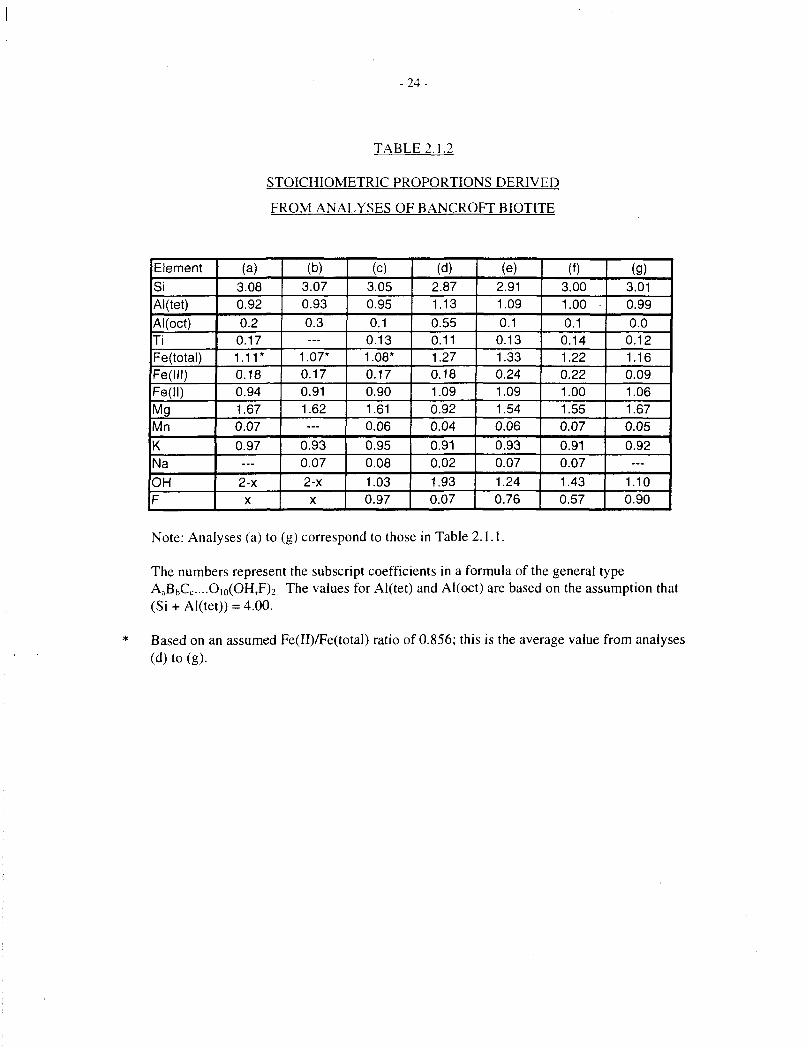
Our own analyses of Bancroft biotite (Taylor and Owen 1995) are in reasonable agreement withthis .formula. Some of the published analyses for this material are compiled in Table 2.1.1, andcorresponding empirical formulae are shown in Table 2.1.2.

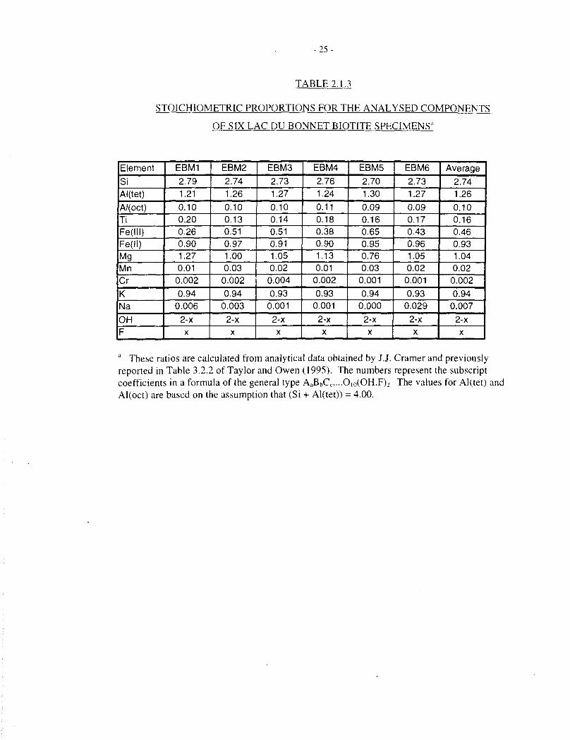
Some of the dissolution and oxygen-consumption experiments described here were performedwith Bancroft biotite, purchased from Wards Scientific. We have also worked with six biotitespecimens that were separated from Lac du Bonnet granite. Calculated stoichiometries of the sixdifferent specimens, based on microprobe analyses and titrimetric determination of theFe(III)/Fe(total) ratio, are shown in Table 2.1.3. The formulae span the range:

Nao.OO-O.O3Ko.93.094Mgo.76-l 27Mno.OI-OO.iFe o.90-0.97Fe O26-O.6.'iCr<o.oiTio.l3-O.2O (3 )

Al l .31-1.38Si2.70-2.7<>0]o(OH)2 ,

with a mean composition of:

NaooiKo94Mgi 04Mnoo2Fe"o93FeI"o46Tio.i6Al|j!6Si2 740io(OH)2 (ignoring fluoride). (4)

This might be compared with the following empirical formula reported for an Australian graniticbiotite from the Snowy Mountains of New South Wales (Fordham 1990):

1 I l l I . (5)

Gilkes and Suddhiprakarn (1979) reported the following formulation from another Australianlocality, near Perth:

(6)

These formulae are also quite highly oxidized, and the former is very iron-rich, in contrast withthe fully reduced formulation reported by Velbel (1985) in his Blue Ridge weathering study:

. (7)

In an experimental alteration study with aims similar to our own, Malmstrom et al. (1995) used abiotite with an analysed composition (Ti and Mn contents unreported):

Ka8oMgo.84Fe"1.1oFe1"o.22Al1.26Si3.i80,o(OH)2 . ' (8)

- 3 -

Because (Al + Si) > 4.00 in formulae (4) and (6) to (8), but not (2) and (5), it would appear thatsome Al is present in the octahedral layer in the Lac du Bonnet and Blue Ridge biotites.However, minor analytical variations can lead to differing conclusions in this respect. Forexample, the analysis of Bancroft biotite by Acker and Bricker (1992) led them to conclude thatit contains a significant amount of octahedral aluminum, whereas the results of Turpault andTrotignon (1994) suggest that this is not the case. Furthermore, substitution of Fe?+ into thetetrahedral layer can influence Al mass balance between the layers. This is not a purelyacademic issue, and may have a significant bearing on interpreting dissolution data. However,for present purposes, the two types of Al (tetrahedral and octahedral) will be lumped in an effortto simplify some of the formulae.

The most variable components in the composition of the Lac du Bonnet biotite specimens are Mgand Fe1"; the concentrations of these components show an inverse correlation, illustrated inFigure 2.1.1. There is little variation in the other major cationic components (K, Al, Fe", Si, Ti),as-seen in Table 2.1.3.

Biotites typically contain some fluoride, which occupies OH sites in the crystal structure, asindicated in Formula (1). We did not obtain fluoride analyses for the Lac du Bonnet specimens,and they are frequently omitted from published analyses.

This discussion of biotite composition is far from comprehensive, and is presented only toillustrate the range of compositions encountered in published dissolution and wethering studies.For a comprehensive discussion of biotite crystal chemistry, see Bailey (1984). The mostimportant difference between the Bancroft and Lac du Bonnet biotites used in the present studyis probably the high and variable Fe"1 content, and correspondingly low Mg, in the Lac duBonnet biotites.

2.2 MINERAL DISSOLUTION GENERALITIES

Fundamental understanding of mineral dissolution kinetics is a daunting topic. The rate of aheterogeneous mineral surface reaction can be described by the general expression (Lasaga1995):

Rate = k0AmineEa/RTaH+

ng(l) . I V 0 ^ A G r ) , (9)

where: k<) is an intensive rate constant with units of moles per unit area per unit time;

Amin is the reactive surface area of the mineral;

Ea is the apparent activation energy for the overall reaction;

aH+ is the activity of hydronium ion (H3O+) in solution;

g(I) represents any effect of ionic strength over and above its influence on dissolved ionactivity coefficients;

jFIai"0' represents the product of all inhibitory or catalytic effects of species in solution(other than hydronium ion, which was separated because it is so commonly studied as a

- 4 -

parameter in dissolution kinetics), expressed as apparent reaction orders, n(i), withrespect to the dissolved species activity;

and/(AGr) accounts for the variation of the rate with the deviation from equilibrium (atwhich AGr = 0).

At a cruder phenomenological level, aluminosilicate minerals commonly display three stages intheir dissolution (Blum and Stillings 1995, Nagy 1995):

(a) A very rapid release of alkali metals or other exchangeable cations (in the case of biotite,primarily potassium).

(b) A stage of relatively fast dissolution, during which all components of the mineraldissolve, albeit not necessarily congruently. This is commonly attributed to the presence of fineparticles or reactive surface zones that have suffered damage during grinding; however, there isevidence that it may be related to the establishment of a steady-state surface composition.

(c) Eventually (after tens, hundreds or even thousands of hours), a slow, steady-statedissolution occurs. This stage is thought to be most relevant to geochemical processes.

The dissolution behaviour (or at least its determination by solution analysis) is furthercomplicated by reprecipitation of some of the components (e.g., Mg, Al, Fe), especially in near-neutral solutions. In addition, the reactive surface area of a mineral may change in the course ofreaction, because of the development of pitted or convoluted reaction fronts. Moreover, in highlyanisotropic minerals like the sheet silicates, the reactive surface area may differ from thegeometric surface area.

In spite of these complexities, various types of sheet-structured silicate minerals (biotite being anexample) display rather similar dissolution rates in near-neutral solutions at 25°C. Nagy (1995)concluded that most sheet silicates have a dissolution rate of 10"'3O±05 mol/m2s (expressed asmoles of [0,o(OH)2] formula unit) at pH 5 and 25°C. The pH dependence (reaction order n withrespect to hydronium ion activity in expression (9)) is typically between 0.1 and 0.5 in the acidicrange, and between -0.1 and -0.5 in the alkaline range; there is usually a broad minimum in therate around pH 6-8.

Nagy (1995) has also compiled information on the temperature dependence of sheet silicatedissolution. The degree of dependence varies with pH, and is typically smallest near neutral pHand greatest at the acidic and alkaline extremes. In general, apparent activation energies are low,rarely exceeding 80 kJ/mol even at extreme pH values.

2.3 THE STOICHIOMETRY OF DISSOLUTION AND ALTERATION

The dissolution of biotite is usually incongruent. The course and rate of reaction depends ontemperature, water chemistry and physical constraints on the system. Therefore, it is not astraightforward matter to infer one feature of the reaction (such as iron availability or oxygenconsumption) from another (such as magnesium or silicon dissolution). Nevertheless, it shou'be possible to extract some useful information from dissolution experiments.

- 5 -

The aluminosilicate products of biotite alteration are typically hydrobiotite (an interstratifiedbiotite/vermiculite phase), vermiculite and kaolinite (Velbel 1985, Acker and Bricker 1992, andreferences therein). Other reported weathering products include halloysite, illite, smectite,chlorite and oxides or hydrous oxides of aluminum and iron(HI) (Gilkes and Suddhiprakarn 1979,Banfield and Eggleton 1988, and references therein).

The conversion of biotite to vermiculite involves the replacement of K+ and any other interlayercations by HiO+ and sometimes Na+, partial oxidation of Fe2+ to Fe3+, and adjustment of the sheetcomposition to accommodate the iron oxidation. The latter adjustment involves release and/oruptake of cationic species, depending on the solution chemistry and the compositions of thebiotite precursor and the vermiculite product. Consequently, a variety of different and usuallycomplex expressions have been proposed to describe biotite alteration. Three examples arediscussed here.

In his Blue Ridge study, Velbel (1985) proposed the following weathering reaction (biotite tovermiculite):

Ko.85Nao.o2Mg,.2Fe"I.3AlI.6sSi2.80,o(OH)2 + 0.19O, + 0.078H+ + 0.31H2O (10)+ 0.016Ca2+ + 0.04Na+ + 0.35A1(OH)2

+ + 0.3Fe(OH)2+ ->

Fe'V^Fe"1, ,A1,2Si28Ol0(OH)20.133Al6(OH),5 + 0.6K+ + 0.1Mg2+ .

In another study of watershed geochemical mass balance, Cleaves et al. (1970) propose theconversion reaction:

6KMg, 5Fe, 5AlSi3O10(OH)2 + 8H2O + 12H2CO3 + 6H+ + 1.5O2 -> (11)4Mg,..,Fe, jAl, 5Si25O)0(OH)2-4H2O + 6K+ + 3Mg2+ + 3Fe2+ + 8SiO2 + 12HCO," + 3H2O .

Acker and Bricker (1992) described the alteration process in their laboratory dissolution studieswith the expression:

g 28.93H+ + 0.7645O2 -» (12)8Ho984Mgl.o94FeIIo.54Fem

0.4i6Al1.25Si2.9.,801o(OH)2 + 0.7Na+ + 9.14K+ + 0.04Ca2+

+ 6.5SiO2 + 3.1Mg2+ + 3.55Fe2+ + 1.95A13+ + 12.529H2O

If these different equations tell us anything, they show that a system containing about tencomponents and only two solid phases (each with variable stoichiometry) has many degrees offreedom. Depending on the mass-conservation constraints, real or imagined, that are imposed onthe reaction, the stoichiometric relationships can vary greatly. For example, the three equations,(10), (11) and (12), represent the release of 0.0, 5.3 and 8.5 moles of silica and -1.84, 0.0 and+2.55 moles of aluminum, respectively, per mole of oxygen consumed. The three equations areconstrained by (i) conservation of Si in the solid phase in eq. (10), (ii) conservation of Al in thesolid phase in eq. (11), and (iii) assumption of a 10:8 mole ratio of biotite to vermiculite in eq.(12).

If we constrain reaction (12) by solid-state aluminum conservation instead of mole ratio, weobtain an alternative expression:

- 6 -

.5g5Fe", o95Fe'"oo25All.i<JSi.,Olo(OH)2 + 15.786H+ + 0.982O2 -» (13)g e 1 " o . 4 i 6 A l l 25Si2.938Oio(OH): + 0.7Na+ + 9.14K+

+ 0.04Ca2+ + 2.02SiO2 + 0.666Mg2+ + 2.252Fe2+ + 3.68H2O

This now represents a limiting case for the biotite-vermiculite conversion, for these twoparticular solid compositions, in which the retention of solid phase is the maximum possiblewithout input of ions (other than H+) from solution.

Another limiting case is congruent dissolution without any precipitation or parallel alteration:

g ) 2 + 10H+ -> (14)0.004Ca2+ + 0.07Na+ + 0.914K+ + 1.585Mg2+ + 1.095Fe2+ + 0.025Fe'+

1

A more general equation for any biotite and vermiculite compositions is:

e"M{Ca(,Na,K(M&/Fe"1,FeI"/Al/,Si602o(OH)4} + (15){2Ma+Mb+Mc+2[M(e+f)-N(s+t)]+?l(Mh-Nu)}H+ + 0.25(M-Mf)O2 ->N{ H(/Mg,Fe"1Fe"I,AlHSi602o(OH)4.vH20} +MaCa2+ + MbNa+ + McK+ + (Md-Nr)Mg2+ + [M(e+f) - N(s+t)]Fe2+ + (Mh-Nu)A?+

+ 6(M-N)SiO2 +{2M-N(v+2)+0.5[2Ma+Mb+Mc+2[M(d+e+f)-N(r+s+t)]+3(Mh-Nu)]}H2O

As it stands, this equation assumes complete removal of exchangeable cations, but it can beeasily modified by changing the solid product composition and the coefficients for the dissolvedcations. It also does not allow for any net release of Fe +, but this can be treated simply by aseparate oxidation step for released Fe2+, such as Reaction (16).

4Fe2+ + O2 + 8OH" -» 2(Fe2Or;cH2O) + (4 - 2JC)H2O (16)

If the precursor and product compositions are known, then the stoichiometry for any limiting caseis readily determined. For example, if Al is conserved in the solid phase then Mh = Nu; for purecongruent dissolution, N = 0, and so forth, whence all the stoichiometric coefficients can bedetermined for the selected case.

Because of the degree of algebraic complexity, this approach is only useful for cases where boththe precursor and product phases are multicomponent phases with variable stoichiometry. Forlimiting cases with simpler product compositions, determination of a reaction stoichiometry isfairly straightforward. For example, consider a hypothetical reaction where congruentdissolution is modified by quantitative oxidation and precipitation of Fe as goethite (a-FeOOH)and Al is precipitated as gibbsite (A1(OH);0:

CauNa,KtMg(/Fe"tFem/AlASi602o(OH)4 + (2a+b+c+2d)H+ + (e/4)O2 -> (17)

aCa2+ + bNa + cK+ + dMg2+ + (e+/)FeOOH + /zAl(OH)., + 6SiO2

+ 0.5(4+2a+b+c+2d-e-f-3h)H2O

This may be a realistic scenario for describing steady-state Mg and Si release in the early stagesof hydrothermal dissolution of biotite, except for the initial rapid K release. It should also benoted that pH changes predicted by equations such as these will be further modified by cation

- 7 -

and surface hydrolysis reactions, so that any attempt to monitor dissolution by pH change shouldbe approached with caution.

2.4 THE LINK BETWEEN POTASSIUM RELEASE AND IRON REDOX CHEMISTRY

There are two fundamental ways in which Fe"+ in biotite can become available for reaction withoxygen: either oxygen diffuses into the biotite and oxidizes the Fe2+ in situ in the solid state, orthe Fe2+ is released from the solid by diffusion or matrix dissolution, and becomes available foroxidation at the biotite surface or in solution. The latter possibility was discussed in Section 2.3;here, we address the alternative mechanism involving oxygen mobility in the biotite.

According to Rancourt et al. (1993), direct solid-state oxidation of biotite occurs only at elevatedtemperatures (above ~400°C) and has a high activation energy (228 kJ/mol). Therefore, thisreaction is not expected to be significant under vault conditions (temperatures <100°C).However, we need to address the possibility that rapid leaching of one component may modifythe matrix diffusion properties sufficiently to make iron more accessible to oxygen ingress. Itturns out that just such a process dominates the weathering of biotite to vermiculite.

Like many other layered silicate minerals, biotite contains interlayer cations (primarily K+) thatare accessible, within certain limits, to ion exchange with H^O+, Na+, or other cations. This haslong been recognized as an important mechanism for potassium release in soils (Newman andBrown 1966 and references therein; Newman 1969, 1970). So long as the aqueous potassiumconcentration remains below a critical level (which depends on both the mica composition andthe solution chemistry), all of the potassium in biotite appears to be accessible for ion exchange(Newman 1969 and references therein). An important consequence of ion exchange is expansionof the interlayer spacing of the crystal structure, which then permits much more rapid interlayerdiffusion of ions and small molecules than in the parent biotite1.

Newman and Brown (1966) specifically investigated the influence of potassium removal on theoxidation of iron in biotite. They extracted potassium from biotite and other micas by reactionwith a solution of sodium chloride and sodium tetraphenylborate (also known as sodiumtetraphenyl boron, NaB^Hs)^ , which precipitates potassium as the insoluble salt, KB(C6H5)4.By suppressing the aqueous potassium concentration in this way, Newman and Brown were ableto extract >95% of the potassium from biotite and other micas within 109 days at 40°C.Concomitant with the potassium release, they observed a substantial increase in the Fe"":Fe" ratioof the product, as compared with the original biotite, for all Fe-rich specimens. For example, aspecimen of Bancroft biotite with an original iron analysis of 16.71 wt.% FeO and 4.03 wt.%Fe2O3 yielded a vermiculite product with 9.44 wt.% FeO and 11.34 wt.% Fe2O.i, which representsoxidation of nearly half of the ferrous iron content to ferric. Although details of the dissolutionmechanism remain open to debate (Acker and Bricker 1992 and references therein), thisexperimental result does not appear to be in doubt.

Knowledge of this link between K+ release and iron redox chemistry, together with the existenceof a critical potassium concentration above which ion-exchange ceases, helps to resolve some

1 Although Na+ is a smaller cation than K+, the replacement of K+ by Na+ in biotite results in an interlayerexpansion, because the sodium ions are accompanied by interlayer water molecules. The interlayer spacingincreases from -10.0 A in biotite to -12.2 A in the alteration product, Na-vermiculite (Newman and Brown1966).

- 8 -

seemingly contradictory results in the literature. In particular, biotite is resistant to alteration inclosed, low-volume systems, even at elevated temperatures (Taylor and Owen 1995, Lin andClemency 1981), but is rapidly altered in open systems (i.e., those that contain a cation sink or inwhich the solution is replenished), even at low temperatures (Malmstrom et al. 1995, Clemencyand Lin 1981, Newman and Brown 1966, Newman 1969). Some reported biotite dissolutionrates are discussed further in Section 2.5.

Surface weathering of biotite likely represents a more open system in this context than alterationin a waste vault, that is, water replenishment rates are expected to be much lower in a waste vaultthan for near-surface groundwaters. Therefore, kinetic data derived from weathering studies maynot be applicable to predicting biotite behaviour in a waste vault. It is also important todetermine the critical potassium concentration above which rapid ion exchange with biotiteceases under waste vault conditions; this concentration is likely to vary strongly withgroundwater salinity.

The situation described above may also influence dissolution kinetics of biotite, because itintroduces the possibility of cation release to the solution from within the crystal, via interlayerdiffusion. Such a mechanism has been proposed for adjustment of the sheet composition in thecourse of dissolution (Newman and Brown 1966; see discussion by Acker and Bricker (1992)).

2.5 SUMMARY OF DISSOLUTION EXPERIMENTS ON BIOTITE

Acker and Bricker (1992) reported a comprehensive study of biotite dissolution. They examinedthe dissolution of Bancroft biotite as a function of pH (3 to 7) at 22 ± 1.5°C in a large series offluidized-bed reactor and flow-through column experiments; solutions were analysed for Si, Fe,Al, Mg and K. The only electrolyte in most of their experiments was apparently the sulphuricacid added to adjust pH; their principal aim was to obtain data relevant to the effects of acidprecipitation on biotite weathering. Most experiments were run under ambient oxygen partialpressure, and a few were run in either de-aerated solution or with added hydrogen peroxide. Thecolumn experiments included both "unsaturated" (i.e., intermittently dried) and "saturated"(continuous) runs. The dissolution of ball-mill-ground and more gently broken biotite flakes wasalso compared.

Although this study was extensive and thorough, it does have two significant limitations. One isthat the biotite was not ultrasonically cleaned to remove fine particles. We have tried to use theprocedure described by Acker and Bricker (1992) to clean ground biotite specimens (i.e.,repeated washing in acetone) and found that it did not adequately remove fines (Taylor andOwen 1995). The second limitation is that the biotite analysis is incomplete (it omits Ti, Mn andF), and the resulting structural formula differs from that proposed by Turpault and Trotignon(1994) sufficiently to influence the interpretation of the dissolution data (i.e., equation (12)).

Acker and Bricker (1992) observed a reaction order for biotite dissolution of 0.34 ± 0.04 withrespect to hydrogen-ion activity. At pH > 4, they interpreted the dissolution in terms of loss ofoctahedral cations and formation of a vermiculite-type product (equation (12) above), whereas atpH 3 the dissolution involved destruction of both the tetrahedral and octahedral layers.Significant Fe loss was observed at pH < 5. At pH 5, they obtained dissolution rates (after initialfast release) of around 3 x 10"'2 mol/m2s for tetrahedral cations (represented by Si) and 1-2 x 10"" mol/nr-s for octahedral cations (represented by Mg). As described in Section 2.1, these

- 9 -

rates have been converted to a molar unit of biotite with 22 anionic charges. The rates aresomewhat higher than indicated by Nagy's generalization about the dissolution of sheet silicates(Section 2.2), and also higher than Velbel's estimate (based on geochemical mass balance) of1.2 x 10" mol/nr-s (Nagy 1995, Velbel 1985). This is possibly related to the use of areplenishing, flow-through system, which would prevent potassium accumulation in solution (seeSection 2.4).

Some of Acker and Bricker's incidental observations are useful in the interpretation of our ownresults. They noted that the biotite contained some CaCOi inclusions, including microscopicmaterial that could not be removed physically. Above pH 5.3, they found that Al concentrationswere at or below the detection limit, and were presumably controlled by precipitation ofA1(OH)> Also at pH > 5.3, Mg was the only cation from the octahedral layer that was found inoutput solutions; Fe was not detected, and its concentration was assumed to be limited byformation of hydrous ferric oxides.

Turpault and Trotignon (1994) investigated the dissolution of Bancroft biotite single crystals indilute HNOj (pH 1.08). Although this medium is too far removed from groundwater for thedissolution rates or mechanism to be relevant to our needs, these authors did obtain someimportant insight into the relative reactivity of sheet edges and cleavage (basal) surfaces in thebiotite structure. They varied the relative amounts of these types of surfaces by varying the cutcrystal geometry, and clearly demonstrated that sheet edges (i.e., lateral surface area) have apreponderant influence on the dissolution process. This is consistent with the findings of Knaussand Wolery (1989) and Taylor and Owen (1995), as well as preliminary microscopic resultsmentioned by Acker and Bricker (1992). It helps to account for some of the differences indissolution rates between ground and broken biotite specimens reported by Acker and Bricker(1992), because the former are expected to have a higher cleavage:edge surface-area ratio(Turpault and Trotignon 1994).

Clemency and Lin investigated the dissolution of phlogopite (an iron-free mica, nominallyKMg3AlSi3Oio(OH)2) in both "open" and "closed" systems at 25°C (Clemency and Lin 1981, Linand Clemency 1981). The open system contained an ion-exchange material to remove dissolvedcations from solution, whereas these cations were allowed to accumulate in solution in the closedsystem. In the open system, they obtained initial linear dissolution rates of 2 x 10"l0 mol/nr-s,after an initial rapid loss of potassium; the pH in this experiment varied between 3 and 5(Clemency and Lin 1981). In the closed system, at pH 5-6, the initially rapid dissolution fell toan apparent steady-state linear value of about 1.3 x 10"13 mol/nr-s after 300 hours (Lin andClemency 1981).

Recently, Malmstrdm et al. (1995) reported an extensive series of both flow-through and batchdissolution experiments on biotite at 25°C and pH values from 2 to 10. They obtained steady-state dissolution rates (after initial fast release) with minimum values in near-neutral solutions ofabout 3x10'" mol/m2-s for Si, 7 x 10"n mol/m2-s for Fe, 2.2 x 10~'2 mol/m2-s for Mg, and2 x 10~12 mol/m2-s for Al; the pH dependence varied between these elements.

3. NEW EXPERIMENTS ON BIOTITE DISSOLUTION

We have previously reported the results of dissolution tests conducted with both Bancroft andLac du Bonnet biotite specimens in 0.01 mol/L NaCl solution at 100, 150 and 200°C for 5 and 20

- 10-

days, with nominal starting pH values of 7 and 11 (Taylor and Owen 1995). Here, we describe aseries of static dissolution tests to measure biotite dissolution in a similar, neutral NaCI solutionfor up to 200 days at 100°C. The tests included Bancroft biotite and four of the Lac du Bonnetbiotite specimens (EBM2, EBM4, EBM5 and EBM6). The Bancroft biotite specimen was a-40/+100 mesh size fraction (nominally 150 to 420 |im); the Lac du Bonnet biotites were areceived as a somewhat narrower size fraction, -44/+60 mesh. The particle size distributionsappeared similar when examined by scanning electron microscopy, but the Bancroft materialconsisted of much thinner flakes than the Lac du Bonnet biotites, and therefore presumably has aproportionately higher basal, as compared with lateral, surface area, (see Sections 2.5 and 3.2.4).Representative scanning electron micrographs of these materials were published and discussedpreviously (Taylor and Owen 1995).

3.1 DESIGN OF CURRENT EXPERIMENTS

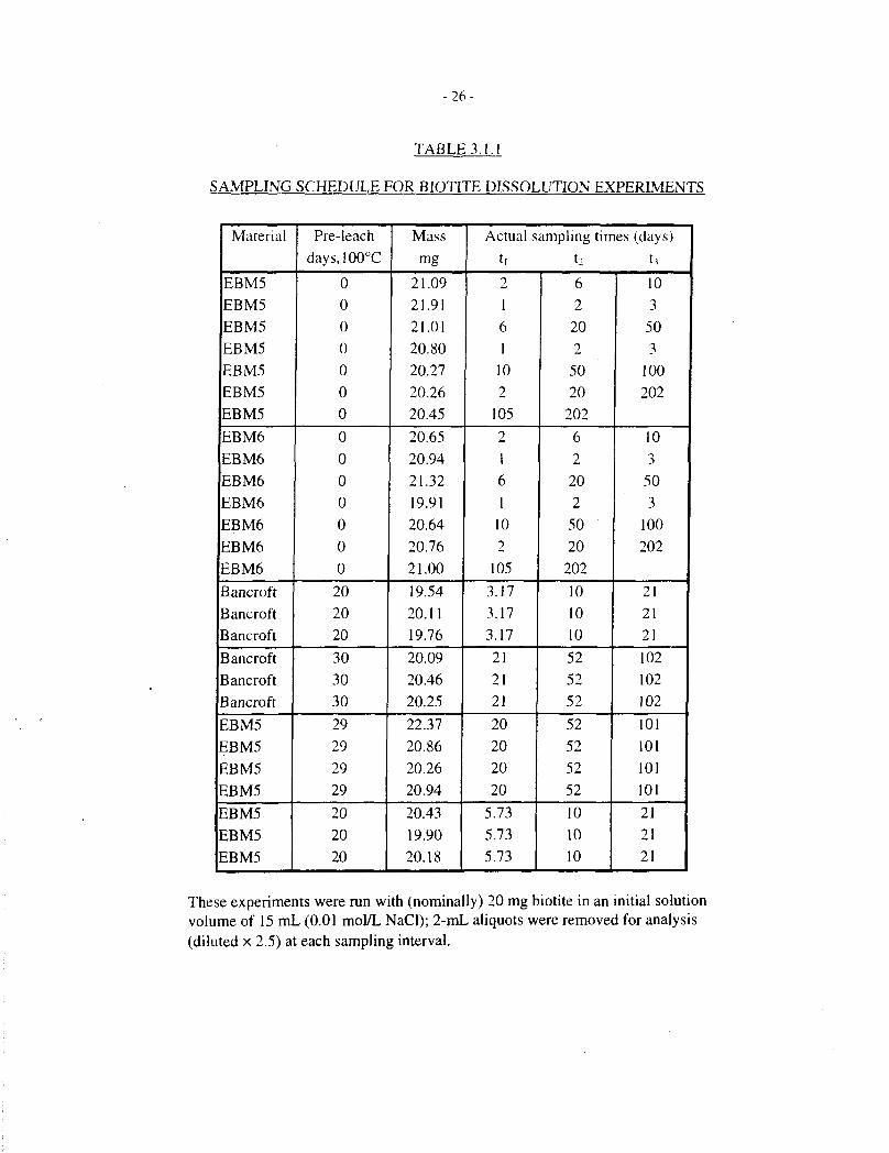
The intent of these tests was to measure steady-state dissolution of biotite in undersaturated,near-neutral solutions. In order to reach steady-state dissolution without reprecipitation of atleast some of the biotite components in a static test, it is necessary to minimize the surface-area-to-volume ratio (SA:V) as far as analytical limitations and acceptable experimental times willallow. This need was reinforced by the limited quantities of separated Lac du Bonnet biotite thatwere easily available (<1 g of each specimen). Tests were therefore run with 20-mg specimensof biotite immersed, unstirred, in 15 mL of 0.01 mol/L NaCI solution in polytetrafluoroethylene-lined vessels. At intervals, 2-mL aliquots of solution were removed for analysis of K by atomicabsorption spectrophotometry and Mg and Si by inductively-coupled plasma spectrophotometry.These aliquots were diluted to 5 mL for analysis. The solutions were not replenished. Based onour earlier results (Taylor and Owen 1995), we did not expect to obtain readily measurablequantities of Al or Fe in solution, therefore these elements were not routinely analysed. In eachrun, the solutions were sampled two or (usually) three times; the sampling schedule and otherexperimental details are shown in Table 3.1.1. A further series of tests was run using 20-mgspecimens of biotite in 8 mL of solution, and analyzing each solution only once, after periods ofup to 100 d. Details of these tests are provided in Table 3.1.2.

All biotite specimens were washed ultrasonically to remove fine particulates before thedissolution tests. The procedure was effective, as previously demonstrated by scanning electronmicroscope examination (Taylor and Owen 1995). Some tests were run on biotite specimenswithout further treatment, whereas others were run on pre-leached specimens (20 to 30 d at100°C, or 20 d at 150°C, in 0.01 mol/L NaCI at 100°C). The main purpose of this treatment wasto reduce the extent of the rapid dissolution phase, and hence permit us to monitor the later stagesof dissolution (in particular, Mg release) for a longer period before saturation occurred. The pre-leached specimens were rinsed and immediately transferred to dissolution tests; no effort wasmade to remove precipitated particles from these specimens.

3.2 RESULTS AND CALCULATIONS

Potassium, magnesium and silicon analyses from the 20-mg/ 15-mL dissolution tests are shown inTables 3.2.1.1, 3.2.1.2, 3.2.2.1, 3.2.2.2, 3.2.3.1 and 3.2.3.2, respectively. To correct for thevariation in solution volume (15 mL initially, 13 mL after the first solution sampling, and 11 mLafter the second), and the minor variation in specimen mass, m, the equivalent times to achieve

- l i -

the same solution concentration at constant solution volume of 15 mL and constant specimenmass of 20 mg were estimated as follows:

t,' = t, (m/20) ,

t2' = t, ' + (15/13)(t2-t,)(m/20) , and

t / = t2' + ( 15/11)(t,-t2)(m/20) ,

where t| , t2 and t.i are the actual total elapsed times for the three samplings and t|\ t2' and t / arethe effective elapsed times. We recognize that these corrections may not be exact. Analyticaldata from the 5O-mg/8-mL tests are included in Table 3.1.2.

3.2.1 Potassium Release

Table 3.2.1.1 shows potassium analyses for solutions contacted with untreated Lac du Bonnetbiotite, specimens EBM5 and EBM6 (20 mg in an initial solution volume of 15 mL), for up to202 days at 100°C. Table 3.2.1.2 shows comparable data forEBM5 and Bancroft biotites, pre-treated in aqueous NaCl for 20 to 30 days at 150°C. All of these data are depicted in Figure3.2.1.1.

The untreated Lac du Bonnet biotites all showed a rapid release (within 1 d) of-1.5-2 mg/L ofpotassium, after which the concentrations remained roughly constant, or increased only siowly,for over 200 d. This behaviour, that is, rapid release up to a limiting value, is consistent with thediscussion in Section 2.4.

The pretreated EBM5 biotite showed only slightly lower potassium release than the untreatedmaterial; the pretreated Bancroft biotite yielded somewhat lower potassium concentrations,scattered between 0.2 and 0.5 mg/L.

A potassium concentration of 0.67 mg/L corresponds to release of about 0.5% of the potassiumcontent of the Lac du Bonnet biotite specimens. We conclude that solid-state oxidation of iron,mediated by potassium extraction (see Section 2.4), will be correspondingly limited in dilute,near-neutral brine in a closed system at 100°C.

Potassium analyses were not included in the later series of dissolution tests with 50-mgspecimens in 8 mL of solution. However, we did perform a separate series of tests in whichBancroft biotite (-40/+100 mesh fraction, ultrasonically cleaned, not pre-leached; nominally10 mg or 70 mg) was contacted with sodium chloride solutions (8 mL) with all nine permutationsof nominal [Na+] = 0.01, 0.1 and 1.0 mol/L, and nominal pH = 3, 7 and 11, for 2 d and 10 d at100°C.

The results of these tests are compiled in Table 3.2.1.3; they confirm earlier reports (see Section2.4) that potassium release depends strongly on sodium concentration, and less strongly on pH(the highest releases occurring in acidic solutions). The potassium concentrations are notstrongly dependent on biotite sample mass, for a given starting solution composition, and releasebetween 2 d and 10 d is evidently much slower than during the initial 2 d. The data were notanalysed further.

- 12-

3.2.2 Magnesium Release

Magnesium release is of particular interest, because Mg2+ occupies the same crystallographicsites (octahedral) in biotite as Fe~+, and hence its dissolution should be an indicator of ironavailability. Earlier tests, however, had shown that magnesium approaches saturation fairly earlyin the dissolution/alteration sequence (although not so early as iron and aluminum). Therelatively low ratios of biotite mass to solution volume in the current tests were chosen so that asignificant fractional release of magnesium (at least a few tenths of one percent) would occurwithin a reasonable time (<100 days) before saturation occurred. In this way, we hoped tomeasure the progress of dissolution beyond the initial rapid release stage expected for allcomponents. This expectation was borne out reasonably well, as discussed below.

Table 3.2.2.1 shows magnesium analyses for solutions contacted with untreated Lac du Bonnetbiotites (EBM5 and EBM6, 20 mg in 15 mL) for up to 202 d at 100°C. Table 3.2.2.2 showscorresponding data for pre-treated EBM5 and Bancroft biotites. Table 3.1.2 includes magnesiumanalyses for solutions contacted with four different Lac du Bonnet biotites (EBM2, EBM4,EBM5 and EBM6; 50 mg in 8 mL), for up to 100 d at 100°C.

Figure 3.2.2.1 depicts the magnesium data for untreated EBM5 biotite, plotted against theeffective time at a constant ratio of biotite mass to solution volume (20 mg: 15 mL), as describedat the beginning of Section 3.2. Figures 3.2.2.2, 3.2.2.3, and 3.2.2.4 show corresponding data foruntreated EBM6, pretreated EBM5, and pretreated Bancroft biotite specimens, respectively.

The untreated EBM5 material (Figure 3.2.2.1) shows a relatively rapid release, up to about0.2 mg/L, over the first 10 d, followed by a slower, roughly linear release up to about 0.3 mg/Lover the ensuing -100 d, after which the concentration levels off. The untreated EBM6 biotite(Figure 3.2.2.2) also shows a rapid initial release of magnesium, but the subsequent data are morescattered. The pre-treated EBM5 biotite (Figure 3.2.2.3) shows a smaller initial, fast release thanthe untreated material, especially for the longer pretreatment, and a more clear-cut subsequentlinear release phase. The pretreated Bancroft biotite (Figure 3.2.2.4) shows qualitatively similarbehaviour, but somewhat faster magnesium release.

Figure 3.2.2.5 shows magnesium release data for four pretreated Lac du Bonnet biotite specimens(50 mg in 8 mL solution) over 100 d at 100°C. These all show a rapid initial release (1 d),followed by a roughly linear release stage (up to 20 d), after which most concentrations level offor drop slightly, indicating that saturation has occurred. The scatter in data between the fourspecimens is within a factor of two of the mean, indicating that biotite dissolution is not verysensitive to differences in composition. The data are discussed further, in terms of fractionalreleases and comparison with silicon, in Section 3.2.4.

3.2.3 Silicon Release

Silicon release data, corresponding to the magnesium data just discussed, are provided in Tables3.2.3.1, 3.2.3.2 and 3.1.2, and Figures 3.2.3.1 to 3.2.3.5. The behaviour of silicon is broadlysimilar to that of magnesium, except that it does not appear to reach saturation in the later stages

- 13-

of the dissolution experiments. The behaviour of magnesium and silicon is best compared interms of fractional release, which is done in the following section.

3.2.4 Comparison of Fractional Release of Magnesium and Silicon

The fractional release of magnesium and silicon (expressed as a percentage of the initial mass ofeach element in the biotite specimens) from untreated EBM5 biotite (20 mg in 15 mL, up to202 d actual elapsed time) is plotted in Figure 3.2.4.1. This figure clearly shows congruentbehaviour of the two elements during both the initial rapid release stage (up to 10 d) and thesubsequent slower, linear release stage (up to 100 d), beyond which the two elements diverge asthe magnesium reaches saturation.

Figure 3.2.4.2 corresponds to Figure 3.2.4.1, except that the data are for untreated SpecimenEBM6. The behaviour is similar to that observed with Specimen EBM5, except that the data aresomewhat more scattered, as noted previously.

Figure 3.2.4.3 shows fractional magnesium and silicon release data for pretreated biotiteSpecimen EBM5 (20 mg in 15 mL, up to 102 d). Both elements show approximately linearrelease kinetics between 20 and 100 days, but their release is not quite congruent, magnesiumdissolution being proportionately a little slower than that of silicon.

Figure 3.2.4.4 shows corresponding fractional magnesium and silicon release data for pretreatedBancroft biotite; in this case, the magnesium release is disproportionately high. We are unable toexplain this observation.

Figures 3.2.4.5 and 3.2.4.6 show fractional magnesium and silicon release data, respectively, forthe four pretreated Lac du Bonnet biotite specimens (EBM2, EBM4, EBM5 and EBM6, 50 mg in8 mL of solution), contacted with aqueous NaCl for up to 100 d. These correspond to theconcentration data depicted in Figures 3.2.2.5 and 3.2.3.5, respectively. Figures 3.2.4.7 to3.2.4.10 compare the magnesium and silicon fractional releases for each specimen. In each case,magnesium releases are proportionately slower than those of silicon, and they approachsaturation after 10 to 20 d, at a fractional release level of about 0.1%.

To compare data obtained from the two series of experiments (20 mg in 15 mL and 50 mg in8 mL), all data for pretreated EBM5 specimens were pooled and plotted on a scale of effectivetime, that is, scaled to 20 mg / 15 mL as described at the beginning of Section 3.2. The data arepresented in Figure 3.2.4.11 (expressed as concentrations) and Figure 3.2.4.12 (with the twoelements normalized by multiplying the magnesium concentration by the initial Si:Mg mass ratioin the biotite).

These figures again illustrate the following stages of dissolution:

(a) Rapid initial release of both magnesium and silicon;

(b) Disproportionately slow magnesium release, as compared with silicon;

(c) Saturation with magnesium in the later stages of dissolution.

- 14-

In addition, deviation of silicon release from linear behaviour beyond 100 d indicates that silicon,too, may be approaching saturation at longer times, or that the dissolution mechanism ischanging.

3.2.5 The Vexatious Question of Surface Area

Theoretical considerations - Any detailed interpretation of solid-dissolution data requires ameasure of the solid surface area. The problem of obtaining a realistic surface area iscompounded in the present case by the highly anisotropic structure and properties of biotite. It iswell established that the dissolution of biotite is dominated by the surface area of platelet edges,as opposed to either the total or basal surface areas (see Section 2.5). Standard methods forsurface area measurement, such as the BET technique, cannot readily distinguish between basaland edge surface areas. Moreover, any estimates based on particle geometry require somemeasure of surface roughness, which is also difficult to measure and likely to differ significantlybetween basal and edge surfaces.

Consider a biotite specimen consisting of disk-shaped particles with radius r and thickness X(measured in (im), density p (in g/cm3), basal roughness xh and edge roughness xe. The mass, M,of one particle is given by:

M = Ttrxp x 10~12 g (the factor of 10"'2 converts |i.m* to cm')

The basal surface area, Ah (two faces of one disk) is:

Ah =2Kr2xhx 10"l2m2 ,

and the edge surface area, Ae, is:

AL, = 2nnxt, x 10 1 2 m2 ,

for a total surface area, A, of:

2nr{rxh + lxt) x 10"'2 m2 .

The specific surface area is then:

2nr(rxh + xx^/nrhp m2/g

= 2(rxh + xxc)/np m2/g .

The specific basal surface area (in m2/g) is 2x>/rp, and the specific edge surface area is 2x<Jrp.

Unfortunately, the attractive simplicity of these expressions is marred by consideration of thephysical reality of surface roughness in a lamellar material such as biotite. Basal roughnessamounts to exposure of additional edge surfaces on the disk face, whereas edge roughness is acombination of jaggedness of the edge itself (i.e., roughness perpendicular to the basal plane)and raggedness of the lamellar edges (i.e., roughness parallel to the basal plane, analagous to astack of torn paper), which exposes additional basal surfaces. This is illustrated schematically

- 15-

by a sketch in Figure 3.2.5.1, and by scanning electron micrographs of actual biotite specimens inFigure 3.2.5.2. The situation is further complicated by changes in the surface area of a specimenduring dissolution, due to the opposing effects of rounding of initial rough features and thedevelopment of etch features (growth of pits, opening of microcracks, etc.). Biotite morphologyis discussed in more detail in an earlier report (Taylor and Owen 1995).

One simple, but rather unsatisfactory, way out of this dilemma is to state that the observeddissolution rates apply to fractured material with particle diameters uniformly distributed in the100 to 500 |im range, and that the rate is likely to vary inversely with biotite particle diameter (asindicated by the expression given above for specific edge surface area).

Calculations on granite-based backfill will be further complicated by the need to estimate therelative fractions of edge and basal surfaces of biotite that are exposed on a fractured rocksurface, or along water-accessible cracks in such rock.

Experimental measurements -Surface-area measurements, using the BET nitrogen-absorptionmethod, were made for most of the biotite and magnetite powders used in this study; results aregiven in Table 3.2.5.1. As expected, our in-house measurements show higher surface areas foreither smaller mesh-size fractions or re-ground material, and substantially lower surface areas,for Lac du Bonnet biotite than for the flakier Bancroft material. There is little variation amongthe six Lac du Bonnet specimens. However, in-house measurements of Bancroft biotite aresignificantly higher (by a factor of 3 to 5) than those obtained by a commercial laboratory forsimilar specimens, or for similar materials studied elsewhere (Acker and Bricker 1992). Atpresent, we are unable to account for these discrepancies. In the following discussion andcalculations, we use an average surface area of 0.84 m7g for the four Lac du Bonnet biotitespecimens used in dissolution studies, and the in-house measurements are used for calculationson oxygen consumption by the Bancroft biotite. This is conservative, in the sense that actualsurface areas may be lower, and hence dissolution and oxygen consumption rates per unit surfacearea may be underestimated.

One additional important finding is that the surface area of finely ground biotite changes onlyslightly after prolonged contact with aqueous sodium chloride solution at 100°C (see Table3.2.5.1).

3.3 DISCUSSION

It only remains to determine what, if anything, useful can be extracted from our biotitedissolution data, with respect to iron availability. The complexity of the dissolution/precipitationprocess indicates that any attempt to model iron availability should be conducted with caution.Nevertheless, the fairly reproducible behaviour of different biotite specimens, as well as theexistence of a significant stage of linear release kinetics (after initial rapid dissolution), indicatethat some non-conservative bounding calculations of iron availability are feasible.

Biotite dissolution rates during the linear release stage were estimated by linear regression ofmagnesium analyses for times up to 20 days in the 5O-mg/8-mL series of experiments with fourdifferent Lac du Bonnet biotites, and from 20 to 100 days for all of the 2O-mg/15-mLexperiments with pretreated Lac du Bonnet biotite specimen EBM5. Results are presented inTable 3.3.1. The rates for the former series ranged from 7.73 to 9.94 x lO"'3 mol/gs for the four

- 16-

different specimens, with an average of (8.7 ± 4.2) x 10"13 mol/g-s (stated error is 2a). The ratederived from the latter series of data is (6.1 ± 1.4) x 10° mol/g-s. These rates are expressed asmoles of biotite, using the '"0,0(01-1)2" formulation.

Using the provisional surface-area value of 0.84 m2/g, we estimate biotite dissolution rates of(10 ± 5) x 10"" mol/nr-s and (7 + 2) x lO"" mol/m2s, respectively. These values can becompared with estimates of about 10" mol/m~s from closed-system experiments or weatheringcalculations for biotite in near-neutral solutions at ambient temperature, as discussed in Sections2.2 and 2.5. A steady-state alteration rate of 10"'~ mol/m2s appears to be reasonable for thepurposes of estimating oxygen consumption under waste-vault conditions, with the caveat thatlower rates may prevail when the solution is saturated with magnesium and/or silicon, or ifalteration products eventually form a protective layer. It should also be recognized thatdissolution rates in complex groundwaters may differ from those in dilute aqueous sodiumchloride solution.

Assuming 0.93 mol Fe2+ per mol biotite (see Table 2.1.3), and consumption of 1 mol of O2 per4 mol of Fe"+ released (e.g., Reaction (16)), we estimate a steady-state oxygen consumption rate(after rapid initial reaction of freshly exposed surfaces) of about 2 x 10'13 mol (O2)/m

2 (biotite)s.

If this rate could be sustained in a waste vault, then oxygen in the backfill would be scavenged inapproximately 50 years (based on the estimates by Johnson et al. (1994) of 0.2 mol of O2 and620 m of biotite per cubic metre of backfill). However, the dissolution rates in our experimentsdeclined after 20 to 100 d, depending on the mass:volume ratios used. Therefore, thesecalculations may overestimate the average rate of oxygen consumption over reaction times ofseveral years. Because of such uncertainties, we have performed additional experiments to try tomeasure directly the consumption of oxygen by biotite and magnetite. These experiments aredescribed in Section 4.

4." DIRECT MEASUREMENT OF OXYGEN CONSUMPTION

Because of the uncertainties in any estimate of biotite dissolution and alteration kinetics, and theavailability of iron thereby deduced, it is important to attempt to measure oxygen consumptiondirectly. Here, we describe such attempts.

4.1 BACKGROUND AND EARLY DIFFICULTIES

The alteration of biotite, and hence the oxidation of its Fe" component, are sufficiently slow andcomplex to be experimentally challenging, as described in the foregoing sections. In order tomeasure oxygen consumption directly and expeditiously, it is therefore desirable to work with arelatively large amount of powdered biotite in a small volume of aerated solution with minimalgas head-space (i.e., maximize SA.V, unlike the situation with dissolution measurements), aswell as minimizing the initial oxygen concentration. Initial tests with small autoclaves(-400 mL), fitted with gas-sampling attachments for mass spectrometric analysis of the covergas, were inconclusive, because the achievable SA.V was too low with the quantities of biotite atour disposal. We also encountered problems with leaking valves because of biotite flakesadhering to the valve stems.

- 17-

Because of these difficulties, we chose to conduct a series of tests in all-glass sealed vesselsfitted with break seals. This was feasible because of the relatively low experimental temperature(100°C). These vessels have a low enough volume (-10 mL) that it should be possible tomeasure oxygen uptake rates as low as 0.1 (amol/d in a 100-d test, with an initial oxygenconcentration of 2 vol.%. Two vessel designs were tested; they are illustrated by a sketch inFigure 4.1.1. Design A was less successful, because it proved more difficult to purge the vesselwith gas mixture without contaminating the seal area with solid, which was transported up thevessel stem by gas bubbles. This contamination led to faulty seals in several cases. Thisproblem was eliminated with the bulbous vessel design, B.

This approach provides an inexpensive way of measuring oxygen consumption by solids inaqueous systems at temperatures near or below 100°C. It has one obvious drawback, however, inthat it relies on a single "all-or-nothing" analysis at the end of the test; the procedure is thereforeboth unforgiving and data-poor (i.e., it does not provide continuous monitoring of oxygen levels).Therefore, these tests should be considered as scoping experiments that will help in the design ofmore elaborate, large-scale tests that may be needed to provide full assurance of oxygenconsumption in a waste vault.

In addition to tests with biotite, we have conducted a series of comparative oxygen-consumptiontests with various magnetite powders. Biotite tests were conducted with various size fractions ofthe Bancroft material, both as-prepared (ground, sieved to obtain the desired mesh fraction, andin some cases ultrasonically cleaned) and pre-leached (20 days at 150°C in 0.01 mol/L NaCl).Magnetite tests were conducted with three types of powder:(a) "Mapico Black" commercial magnetite powder (Columbian Chemicals Canada Ltd.,

Hamilton ON), as received;(b) Mapico commercial magnetite powder, freshly reduced in a CO/CO2 atmosphere at

800°C for 32 minutes. The gas composition was adjusted while heating and cooling, soas to remain within the magnetite stability field at all temperatures above 400°C

(c) Johnson-Matthey high-purity magnetite powder (99.999% stated purity, metals basis).

4.2 EXPERIMENTAL

Glass-blown vessels were constructed according to designs A and B. Solid biotite or magnetitewas weighed into the dry vessel, followed by a measured quantity of distilled, deionized water.The aqueous phase was purged with an Ar-2% O2 gas mixture2 for at least 1 h, then the vesselwas flame-sealed at the point indicated in Figure 4.1.1. The vessel was then placed in a forced-air convection oven at 100°C for the duration of the test (up to 100 d). It was then removed andcooled, and the gas phase was analysed by mass spectrometry, by breaking the break-seal with amagnetic bar once the vessel was mounted on the mass-spectrometer inlet and the systemevacuated.

4.3 RESULTS

Results of the gas analyses from the experimental runs are shown in Table 4.3.1. In addition tomeasuring oxygen consumption, the analysis provides the following information:

2 Nominal composition; analysed composition, 3.07 mol % Oi, balance Ar

- 18-

(a) Analysis of Ar and N2 provides assurance that the vessel was adequately purged andremained leak-tight up to the point of analysis.

(b) Evolution of H2 and CO2 can also be measured.

4.4 DISCUSSION

The rate of oxygen consumption in these experiments was calculated using a spreadsheet(Microsoft Excel, version 5.0), as follows:

(a) The initial gas-phase composition was assumed to be 3.07 mol % O2, 96.93 mol % Ar, and itwas assumed to be in equilibrium with the aqueous phase at 21 °C when loaded;

(b) The gas volume, and hence the quantity (moles) of gaseous O2 and Ar, were calculated fromthe measured total volume of the individual vessel, less the volumes of water and solid reagent(based on theoretical densities of 5.18 g/cm3 for magnetite, 2.9 g/cm' for biotite, 2.7 g/cm3 forgranite and 0.998 g/cm for water).

(c) The initial aqueous Ar and O2 concentrations were calculated from the following solubilitiesof the pure gases in water at atmospheric pressure (101.3 kPa) and an ambient temperature of21°C, from Gevantman (1995):

Ar solubility (mole fraction) = 2.70 x 10'5 ;O2 solubility (mole fraction) = 2.46 x 10'5.

(d) The total initial quantity (moles) of O2 was calculated from (b) and (c). No correction wasmade for loss of gas due to expansion when the side-arm was sealed.

(e) The fraction of O2 remaining at the end of each run was calculated as follows:

Fraction remaining = (%O2 final)(%Ar initial)/(%O2 initial)(%Ar final)= (%O2 final)/(%Ar final) x 96.93/3.07

(f) The quantity of oxygen consumed was converted to an average consumption rate per gram orsquare metre of solid reagent. In many cases, this value was an upper or lower limit. Results ofthese calculations are shown in Table 4.3.2.

One complication in the oxygen consumption by untreated biotite is the evolution of anapproximately equivalent quantity of carbon dioxide (see Table 4.3.1). This raised the possibilityof oxygen consumption by organic impurities rather than the biotite itself; however, biotite doesnot normally contain any significant quantities of organic material. Bancroft biotite (in commonwith other biotites) is known to contain microscopic calcium carbonate inclusions (Acker andBricker 1992), and it is more likely that the CO2 evolution arose from dissolution of theseinclusions. The levels of CO2 were much lower in tests involving pre-leached biotite, ascompared with freshly ground material, which is consistent with this explanaiion.

- 19-

The same runs that yielded significant levels of C02 also led to some hydrogen evolution (Table4.3.1). The reason for this is obscure; it may simply be an artifact arising from traces of metallicimpurities from the grinding process.

Calculated rates of oxygen consumption by Bancroft biotite, as measured in these experiments(Table 4.3.2) range from about 6 x 10"'4 mol/m~s for some tests with untreated -40/+I00 meshmaterial to a lower limit of 1.5 x 10"" mol/m2s for untreated -100-mesh material. Rates for pre-leached materials are close to 1 x 10"" mol/m2s. This is similar to the rate of-2 X 10"" mol/m" sestimated for Lac du Bonnet biotite on the basis of magnesium dissolution measurements;indeed, the results are gratifyingly similar. The lower value for the Bancroft biotite can beattributed in part to a higher contribution of basal surfaces to its total surface area.

Preliminary tests on crushed granite specimens indicated oxygen consumption rates also in therange of 10"" mol/nr-s, but this should be regarded as a preliminary value. Given that iron-containing minerals constitute only a small fraction of granite, this value is somewhat higher thanexpected.

Experiments with magnetite were initially conducted with three types of magnetite. When itbecame apparent that the lowest purity material (as-received "Mapico Black") was a veryeffective oxygen scavenger, work on high-purity and freshly reduced materials was not pursued.Oxygen was >99% consumed in all tests with magnetite, even in a 10-day run with just 0.2 g ofsolid, indicating an oxygen consumption rate of >6 x 10"'2 mol/m2s, i.e., approaching two ordersof magnitude faster than biotite. This applied to material that had been exposed to air, and thuswould be expected to be already partly oxidized to Fe2O, on the surface (Taylor and Owen 1993and references therein).

5. CONCLUSIONS AND RECOMMENDATIONS

Dissolution measurements on Lac du Bonnet biotite in neutral 0.01 mol/L aqueous sodiumchloride solution at 100°C indicate that, after an initial rapid dissolution stage, the biotitedissolves at a rate of 6-10 x 10"'3 mol/g-s, or ~10"12 mol/m2-s, until the net dissolution ratedeclines as the solution approaches saturation with magnesium (the solubility-controlling phaseis not known). This rate is based on the "On" formula, i.e., the nominal formulaK(Mg,Fe)3(Al,FeSi?Oio(OH,F)2). We estimate from this that Lac du Bonnet biotite can consumeoxygen at a rate of about 2 x 10"13 mol/nr-s; this in turn yields an estimated time of about 50years for consumption of oxygen entrained in granite-based backfill in a nuclear fuel waste vaultof the type envisaged in Canada. Direct measurements of oxygen consumption by Bancroftbiotite are consistent with these findings. Oxygen consumption by magnetite is considerablyfaster than by biotite, but possible consequences of adding magnetite to buffer or backfillmaterials have not been addressed here.

The uncertainties in these estimates of oxygen consumption are large, and difficult to evaluatewithout performing more realistic tests with simulated backfill material. The largestuncertainties lie in the surface area measurements, in particular the estimation of the edge surfacearea that is thought to control dissolution and reactivity with oxygen. The available surface areafor biotite dissolution and alteration will further depend on the extent of cracking in granitefragments, as well as their size and geometry and the nature of the exposed biotite surfaces (edge

- 2 0 -

or basal). Caution is also obviously needed in extrapolating our results to long times and todifferent groundwater compositions.

We recommend that any further experiments on oxygen consumption by biotite, granite,magnetite or other materials be conducted on a larger scale, under conditions more closelyresembling a nuclear fuel waste vault. The estimated oxygen consumption rates presented herecan be used to scale and design such an engineering-scale test.

ACKNOWLEDGEMENTS

In its early stages, this work was cofunded by AECL and Ontario Hydro under the auspices ofCOG Working Party 41; more recently, it was funded entirely by Ontario Hydro. We thankH.G. Delaney for the mass-spectrometric gas analyses, K. Wazney and E. Rochon for thesolution analyses, and M. Tateishi for the surface-area measurements. We are also grateful toJ.J. Cramer for the Lac du Bonnet biotite specimens and analytical data. Many colleagues atAECL and Ontario Hydro have provided helpful comments; in particular, we thank J.J. Cramerand J. McMurry for reviewing this report.

REFERENCES

Acker, J.G. and O.P. Bricker. 1992. The influence of pH on biotite dissolution and alterationkinetics at low temperature. Geochimica et Cosmochimica Acta 56, 3073-3092.

Bailey, S.W. (editor). 1984. Micas. Reviews in Mineralogy, Volume 13. Mineralogical Societyof America.

Banfield, J.F. and R.A. Eggleton. 1988. A transmission electron microscope study of biotiteweathering. Clays and Clay Minerals 36, 47-60.

Blum, A.E. and L.L. Stillings. 1995. Feldspar dissolution kinetics. In Chemical WeatheringRates of Silicate Minerals (A.F. White and S.L. Brantley, editors), Reviews in Mineralogy,Volume 31, 291-351, Mineralogical Society of America.

Cleaves, E.T., A.E. Godfrey and O.P. Bricker. 1970. Geochemical mass balance of a smallwatershed and its geomorphic implications. Geological Society of America Bulletin 81,3015-3032.

Clemency, C.V. and F.-C. Lin. 1981. Dissolution kinetics of phlogopite. II. Open system usingan ion-exchange resin. Clays and Clay Minerals 29, 107-112.

Fordham, A.W. 1990. Formation of trioctahedral illite from biotite in a soil profile over granitegneiss. Clays and Clay Minerals 38, 187-195.

Gevantman, L. 1995. Solubility of selected gases in water. In CRC Handbook of Chemistryand Physics, 76th Edition, 6-3 to 6-6, CRC Press, Boca Raton, Florida.

-21 -

Gilkes, R.J. and A. Suddhiprakarn. 1979. Biotite alteration in deeply weathered granite. I.Morphological, mineralogical, and chemical properties. Clays and Clay Minerals 27, 349-360.

Gilkes, R.J., R.C. Young and J.P. Quirk. 1972. The oxidation of octahedral iron in biotite.Clays and Clay Minerals 20, 303-315.

Gilkes, R.J., R.C. Young and J.P. Quirk. 1973. Artificial weathering of oxidized biotite. I.Potassium removal by sodium chloride and sodium tetraphenylboron solutions. Soil ScienceSociety of America Proceedings 37, 25-28.

Hancox, W.T. and K. Nuttall. 1991. The Canadian approach to safe permanent disposal ofnuclear fuel waste. Nuclear Engineering and Design 129, 109-117.

Johnson, L.H., D.M. LeNeveu, D.W. Shoesmith, D.W. Oscarson, M.N. Gray, R.J. Lemire andN.C. Garisto. 1994. The disposal of Canada's nuclear fuel waste: the vault model for postclosureassessment. Atomic Energy of Canada Limited Report, AECL-10714, COG-93-4.

Knauss, K.G. and T.J. Wolery. 1989. Muscovite dissolution kinetics as a function of pH andtimeat70°C. Geochimica et Cosmochimica Acta 53, 1493-1501.

Lasaga, A.C. 1995. fundamental approaches in describing mineral dissolution and precipitationrates. In Chemical Weathering Rates of Silicate Minerals (A.F. White and S.L. Brantley,editors), Reviews in Mineralogy, Volume 31, 23-86, Mineralogical Society of America.

Lin, F.-C. and C.V. Clemency. 1981. Dissolution kinetics of phlogopite. I. Closed system.Clays and Clay Minerals 29, 101-106.

Malmstrom, M., S. Banwart, L. Duro, P. Wersin and J. Bruno. 1995. Biotite and chloriteweathering at 25°C: The dependence of pH and (bi)carbonate on weathering kinetics, dissolutionstoichiometry, and solubility; and the relation to redox conditions in granitic aquifers. SvenskKarnbranslehantering AB (Swedish Nuclear Fuel and Waste Management Co.) Technical Report,SKB-95-01.

Nagy, K.L. 1995. Dissolution and precipitation kinetics of sheet silicates. In ChemicalWeathering Rates of Silicate Minerals (A.F. White and S.L. Brantley, editors), Reviews inMineralogy, Volume 31, 173-233, Mineralogical Society of America.

Newman, A.C.D. 1969. Cation exchange properties of micas. I. The relation between micacomposition and potassium exchange in solutions of different pH. Journal of Soil Science 20,357-373.

Newman, A.C.D. 1970. The synergetic effect of hydrogen ions on the catio.i exchange ofpotassium in micas. Clay Minerals 8, 361-373.

Newman, A.C.D. and G. Brown. 1966. Chemical changes during the alteration of micas. ClayMinerals 6, 297-310."

- 2 2 -

Rancourt, D.G., P. Tume and A.E. Lalonde. 1993. Kinetics of the (Fe2+ + OH")mica -»(Fe1+ + O2)mica + H oxidation reaction in bulk single-crystal biotite studied by Mossbauerspectroscopy. Physics and Chemistry of Minerals 20, 276-284.

Shoesmith, D.W., F.King and B.M.Ikeda. 1995. An assessment of the feasibility of indefinitecontainment of Canadian nuclear fuel wastes. Atomic Energy of Canada Limited Report,AECL-10972, COG-94-534.

Taylor, P. and D.G. Owen. 1993. Oxidation of magnetite in aerated aqueous media. AtomicEnergy of Canada Limited Report, AECL-10821, COG-93-81.

Taylor, P. and D.G. Owen. 1995. Reaction of biotite with aerated aqueous solutions: apreliminary report on the effects of temperature, pH and biotite composition. Atomic Energy ofCanada Limited Report, RC-1364, COG-I-95-022.

Turpault, M.-P. and L. Trotignon. 1994. The dissolution of biotite single crystals in diluteHNO3 at 24°C: evidence of an anisotropic corrosion process of micas in acidic solutions.Geochimica et Cosmochimica Acta 58, 2761-2775.

Velbel, M.A. 1985. Geochemical mass balances and weathering rates in forested watersheds ofthe southern Blue Ridge. American Journal of Science 285, 904-930.

- 2 3 -

TABLE 2.1.1

PUBLISHED ANALYSES FOR BANCROFT BIOTITE

Component

SiO,FeOFe,O,M.aOANO,K,OTiO-,MnONa-,0CaOLi,OZnOCr,O,F

aH.ODrying LossIgnit'n LossTOTAL

Bancroft(a)

38.418.31*

_..13.9512.259.422.781.08<0.5<0.1.._...___......- .

0.100.83

>97.1

Bancroft(b)

40.64...

20.19*14.3813.699.69—

. ...0.490.05....—....... . ..... . .. . .

97.1

Bancroft(c)

38.6518.18*

...13.6911.099.452.220.900.52............

3.870.08...__....

98.0

Bancroft(d)

37.617.13.078.1218.69.391.920.650.140.54—......

0.27.........

1.5999.0

Bancroft(e)

37.3316.714.0313.2012.539.312.150.930.490.45.........

3.06......

0.141.16

100.21**

Bancroft(f)

38.415.373.7113.311.79.132.31.000.490.160.1110.085

...2.30—1.1......

99.2

Bancroft(?)

39.0516.501.62

14.5011.069.342.090.71....... . .......

3.68

...

...

...

98.55

* When Fe oxidation state was not determined, all Fe is reported as FeO or FeiO.v** Corrected for partial duplication of fluorine analysis and ignition loss(a) Whiteshell Laboratories analysis, by X-ray fluorescence using synthetically matched

standards. Drying and ignition losses were determined by heating at HOC and 1000C,respectively. Mossbauer spectroscopy indicates 8% of Fe is Fe + in Bancroft biotite.

(b) Acker and Bricker (1992); wet chemical analysis.(c) Rancourt et al. (1993); microprobe analysis.(d) Newman (1969), Specimen B6.(e) Newman and Brown (1966).(0 Gilkesetal. (1972).(g) Turpault and Trotignon (1994), wet analysis figures; the authors also report analyses by

quantitative energy-dispersive X-ray analysis.

- 2 4 -

TABLE2.1.2

STOICHIOMETRIC PROPORTIONS DERIVED

FROM ANALYSES OF BANCROFT BIOTITE

ElementSiAl(tet)Al(oct)TiFe(total)Fe(lll)Fe(ll)MgMnKNaOHF

(a)3.080.920.2

0.171.11*0.180.941.670.070.97—

2-xX

(b)3.070.930.3—

1.07*0.170.911.62...

0.930.072-x

X

(c)3.050.950.10.131.08*0.170.901.610.060.950.081.030.97

(d)2.871.130.550.111.270.181.090.920.04

0.910.021.930.07

(e)2.911.090.10.131.330.241.091.540.060.930.071.240.76

(f)3.001.000.10.141.220.221.001.550.070.910.071.430.57

(g)3.010.990.0

0.121.160.091.061.670.050.92...

1.100.90

Note: Analyses (a) to (g) correspond to those in Table 2.1.1.

The numbers represent the subscript coefficients in a formula of the general typeAaBbCc....Oio(OH,F)2 The values for Al(tet) and Al(oct) are based on the assumption that(Si + Al(tet)) = 4.00.

* Based on an assumed Fe(II)/Fe(total) ratio of 0.856; this is the average value from analyses(d) to (g).

- 2 5 -

TABLE2.1.3

STOICHIOMETRIC PROPORTIONS FOR THE ANALYSED COMPONENTS

OF SIX LAC DU BONNET BIOTITE SPECIMENS'

Element

SiAl(tet)

Al(oct)TiFe(lll)Fe(ll)MgMn

Cr

K

Na

OHF

EBM12.791.210.100.200.260.901.270.01

0.0020.94

0.0062-x

X

EBM22.741.260.100.130.510.971.000.03

0.0020.94

0.0032-x

X

EBM32.731.270.100.140.510.911.050.02

0.0040.93

0.0012-x

X

EBM4

2.761.240.110.180.380.901.130.01

0.0020.93

0.0012-x

X

EBM52.701.300.090.160.650.950.760.03

0.0010.94

0.0002-x

X

EBM6

2.731.270.090.170.430.961.050.020.0010.93

0.0292-x

X

Average2.741.260.100.160.460.931.040.020.0020.94

0.0072-x

X

a These ratios are calculated from analytical data obtained by J.J. Cramer and previouslyreported in Table 3.2.2 of Taylor and Owen (1995). The numbers represent the subscriptcoefficients in a formula of the general type AaBbCc....O|o(OH,F)2 The values for Al(tet) andAl(oct) are based on the assumption that (Si + Al(tet)) = 4.00.

-26 -

TABLE 3.1.1

SAMPLING SCHEDULE FOR BIOTITE DISSOLUTION EXPERIMENTS

Material

EBM5EBM5EBM5EBM5EBM5EBM5EBM5

EBM6EBM6EBM6EBM6EBM6EBM6EBM6

BancroftBancroftBancroft

BancroftBancroftBancroft

EBM5EBM5EBM5EBM5

EBM5EBM5EBM5

Pre-Ieachdays,100°C

0

0

0

0

0

0

0

0

0

0

0

00

0

20

2020

30

30

30

29

29

29

29

20

20

20

Massmg

21.0921.9121.0120.8020.2720.2620.45

20.6520.9421.3219.9120.6420.7621.00

19.5420.1119.76

20.0920.4620.25

22.3720.8620.2620.94

20.4319.9020.18

Actual sampling times (days)

ti

21

61

10

2

105

2

1

6

1

10

2

105

3.173.173.17

212121

20

20

20

20

5.735.735.73

t2 t.,

62

202

50

20

202

6

2

20

2

5020

202

10

10

10

525252

52525252

10

10

10

10

3

503

100

202

10

3

503

100202

21

21

21

102

102

102

101

101

101

101

212121

These experiments were run with (nominally) 20 mg biotite in an initial solutionvolume of 15 mL (0.01 mol/L NaCl); 2-mL aliquots were removed for analysis(diluted x 2.5) at each sampling interval.

- 2 7 -

TABLE 3.1.2

DETAILS OF FURTHER BIOTITE DISSOLUTION EXPERIMENTS

EBM2mass (mg)K (mg/L)Mg (mg/L)Si (mg/L)EBM4mass (mg)K (mg/L)Mg (mg/L)Si (mg/L)

EBM5mass (mg)K (mg/L)Mg (mg/L)Si (mg/L)

EBM6mass (mg)K (mg/L)Mg (mg/L)Si (mg/L)

1.06

49.61.11

0.1280.892

52.240.91

0.1650.652

53.721.19

0.0880.663

46.951.21

0.0670.677

Duration of dissolution test5

50.941.39

0.3351.3

51.381.21

0.1930.842

50.321.65

0.1610.865

50.532.07

0.1140.831

9

46.821.76

0.3621.54

50.151.60

0.1971.12

47.893.13

0.1480.972

50.652.00

0.1531.06

20

48.21—

0.3572.69

52.63...

0.4531.71

51.26...

0.2891.66

53.14...

0.2801.53

days)50

51.221.68

0.3363.30

48.911.37

0.4382.32

49.931.38

0.3232.09

49.30.97

0.2851.80

102

50.642.410.2113.68

51.551.72

0.6032.8

492.00

0.2822.41

48.771.87

0.3652.16

These experiments were run with (nominally) 50 mg biotite in 8 mL of 0.01 mol/LNaCl); 7 mL of solution was recovered for analysis (undiluted) at the end of each run.

TABLE 3.2.1.1

POTASSIUM ANALYSES FROM DISSOLUTION EXPERIMENTS

WITH BIOTITE, WITHOUT PRE-LEACHING

Sample

designation

BlankBlank

EBM5EBM5EBM5EBM5EBM5EBM5iiBM5

EBM6EBM6EBM6EBM6EBM6EBM6EBM6

wt.% K,O

9.639.639.639.639.639.639.63

9.639.639.639.639.639.639.63

Mass(mg)

00

21.0921.9121.0120.8020.2720.2620.45

20.6520.9421.3219.9120.6420.7621.00

1

0.6

0.62

0.57

0.59

Potassium

2

0.660.71

0.67

0.17

0.60.62

0.64

0.51

3

0.77

0.65

0.65

0.67

(mg/L) at indicated time i

6

0.67

0.7

0.98

0.62

10

——

0.62

0.59

0.63

0.44

20

—

0.61

—

0.48

days), diluted x2.5

50

[0.01][0.03]

0.55

0.6

0.62

0.44

100

[0.04][0.07]

0.65

0.51

105

0.92

0.75

202

0.7540.864

0.6920.892

TABLE 3.2.1.2

POTASSIUM ANALYSES FROM DISSOLUTION EXPERIMENTS WITH PRE-LE ACHED BIOTITE

Sample

designation

BancroftBancroftBancroft

BancroftBancroftBancroft

Blank

EBM5EBM5EBM5EBM5

EBM5EBM5EBM5

Leaching

period

20 d20 d20 d30 d30 d30 d

29 d29 d29 d29 d

20 d20 d20 d

Mass

(mg)

19.5420.1119.76

20.0920.4620.25

22.3720.8620.2620.94

20.4319.9020.18

K (mg/L) at indicated time, diluted x2.576h

0.2240.3380.204

137.5h

0.5360.5200.496

lOd

0.340.3720.262

0.5160.5420.512

20d

0.470.5560.5460.538

21d

0.410.4040.276

0.2320.2160.406

0.5160.4860.546

52d

0.2720.2920.294

0.046

0.510.550.560.65

lOld

0.560.630.660.62

102d

0.480.450.46

0.029

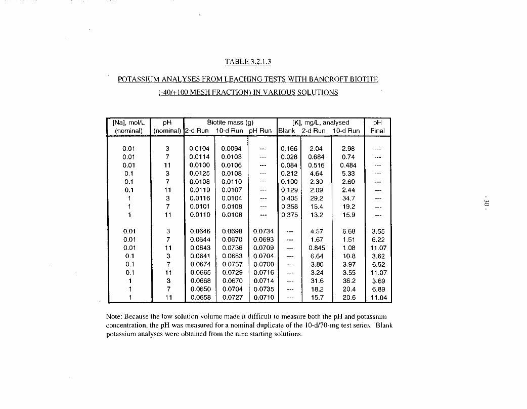
TABLE 3.2.1.3

POTASSIUM ANALYSES FROM LEACHING TESTS WITH BANCROFT BIOTITE

(-40/+100 MESH FRACTION) IN VARIOUS SOLUTIONS

[Na], mol/L(nominal)

0.010.010.010.10.10.1111

0.010.010.010.10.10.1111

pH(nominal)

371137113711

371137113711

Biotite mass (g)2-d Run

0.01040.01140.01000.01250.01080.01190.01160.01010.0110

0.06460.06440.06430.06410.06740.06650.06680.06500.0658

10-dRun pH Run

0.00940.01030.01060.01080.01100.01070.01040.01080.0108

0.06980.06700.07360.06830.07570.07290.06700.07040.0727

...—...——......——

0.07340.06930.07090.07040.07000.07160.07140.07350.0710

[K]Blank

0.1660.0280.0840.2120.1000.1290.4050.3580.375

...

...—...............

mg/L, analysed2-d Run

2.040.6840.5164.642.302.0929.215.413.2

4.571.67

0.8456.643.803.2431.618.215.7

10-dRun

2.980.740.4845.332.602.4434.719.215.9

6.681.511.0810.83.973.5536.220.420.6

PHFinal

...

...—............—

3.556.2211.073.626.5211.073.696.8911.04

Note: Because the low solution volume made it difficult to measure both the pH and potassiumconcentration, the pH was measured for a nominal duplicate of the 10-d/70-mg test series. Blankpotassium analyses were obtained from the nine starting solutions.

o

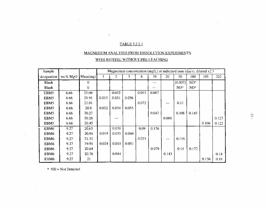
TABLE 3.2.2.1

MAGNESIUM ANALYSES FROM DISSOLUTION EXPERIMENTS

WITH BIOTITE, WITHOUT PRE-LEACHING

Sample

designation

BlankBlank

EBM5EBM5EBM5EBM5EBM5EBM5EBM5

EBM6EBM6EBM6EBM6EBM6EBM6EBM6

wt.% MgO

6.666.666.666.666.666.666.66

9.279.279.279.279.279.279.27

Mass(mg)

00

21.0921.9121.0120.820.2720.2620.45

20.6520.9421.3219.9120.6420.76

21

Magnesium concentration (

1

0.013

0.022

0.019

0.024

2

0.0320.051

0.034

—

0.0310.035

0.045

0.044

3

0.056

0.055

0.044

0.051

6

0.053

0.072

0.09

0.071

mg/L) a

10

——

0.087

0.047

0.176

0.079

t indicated time (days), diluted x2.

20

—

0.088

—

0.143

50

[0.007]ND*

0.11

0.108

0.116

0.14

100

ND*ND*

0.145

0.172

105

0.106

0.156

5

202

0.1270.122

0.140.18

* ND = Not Detected

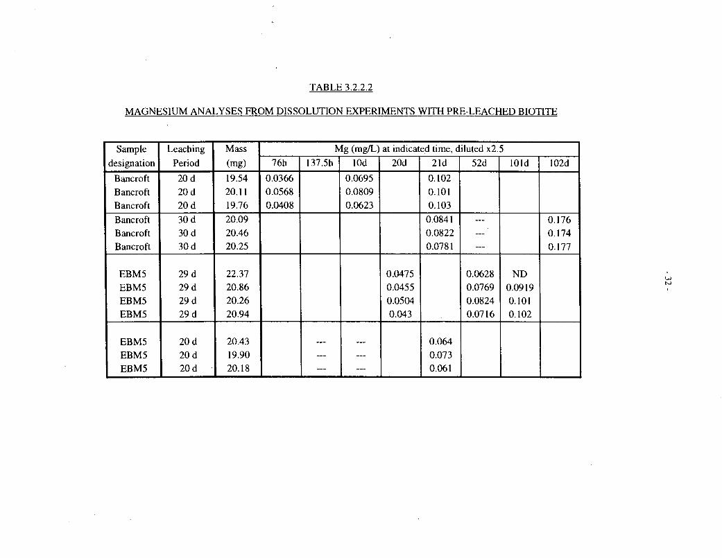
TABLE 3.2.2.2

MAGNESIUM ANALYSES FROM DISSOLUTION EXPERIMENTS WITH PRE-LEACHED BIOTITE

Sample

designation

BancroftBancroftBancroft

BancroftBancroftBancroft

EBM5EBM5EBM5EBM5

EBM5EBM5EBM5

Leaching

Period

20 d20 d20 d30 d30 d30 d

29 d29 d29 d29 d

20 d20 d20 d

Mass

(mg)

19.5420.1119.76

20.0920.4620.25

22.3720.8620.2620.94

20.4319.9020.18

Mg (mg/L) at indicated time, diluted x2.5

76h

0.03660.05680.0408

137.5h

—

lOd

0.06950.08090.0623

—

20d

0.04750.04550.05040.043

21d

0.1020.1010.103

0.08410.08220.0781

0.0640.0730.061

52d

0.06280.07690.08240.0716

lOld

ND0.09190.1010.102

102d

0.1760.1740.177

TABLE 3.2.3.1

SILICON ANALYSES FROM DISSOLUTION EXPERIMENTS

WITH BIOTITE, WITHOUT PRE-LEACHING

Sample

designation

BlankBlank

EBM5EBM5EBM5EBM5EBM5EBM5EBM5

EBM6EBM6EBM6EBM6EBM6EBM6EBM6

wt. %SiO2

35.3635.3635.3635.3635.3635.3635.36

35.9735.9735.9735.9735.9735.9735.97

Mass(mg)

00

21.0921.9121.0120.8020.2720.2620.45

20.6520.9421.3219.9120.6420.7621.00

Silicon concentration (mg/L) after

1

0.075

0.122

0.098

0.125

2

0.1580.13

0.163

0.041

0.1530.149

0.193

0.184

3

0.164

0.261

0.208

0.24

6

0.24

0.216

0.29

0.309

10

...—

0.325

0.22

0.482

0.307

indicated time (days), diluted x2.5

20

—

0.35

—

0.498

50

ND*ND*

0.445

0.472

0.508

0.573

100

ND*ND*

0.626

0.734

105

0.573

0.755

202

0.7420.719

0.7160.803

* ND = Not Detected.

TABLE 3.2.3.2

SILICON ANALYSES FROM DISSOLUTION EXPERIMENTS WITH PRE-LEACHED BIOTITE

Sample

designation

Bancroft3

BancroftBancroft

BancroftBancroftBancroft

EBM5EBM5EBM5EBM5

EBM5EBM5EBM5

Leaching

period

20 d20 d20 d

30 d30 d30 d

29 d29 d29 d29 d

20 d20 d20 d

Mass

(mg)

19.5420.1119.76

20.0920.4620.25

22.3720.8620.2620.94

20.4319.9

20.18

Si (mg/L) at indicated time, diluted x2.5

76h

0.104<0.0850.093

—

137.5h lOd

0.1710.1400.160

—

20d

0.2890.2970.2480.269

21d

0.2400.2070.245

0.2310.2460.221

0.2710.2930.285

52d

—

0.4160.4070.3830.317

lOld

0.5720.5390.5380.534

102d

0.5220.5190.501

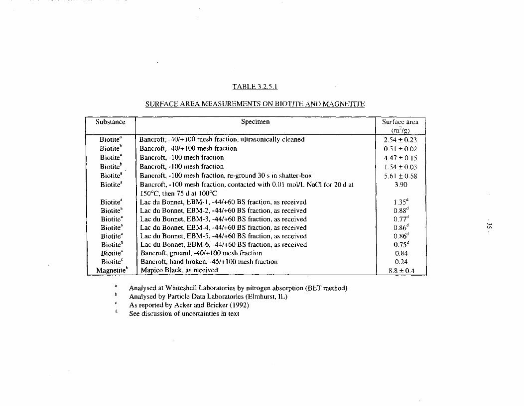
TABLE 3.2.5.1

SURFACE AREA MEASUREMENTS ON BIOTITE AND MAGNETITE

Substance

Biotite"Biotiteb

Biotite"Biotite"Biotitea

Biotitea

Biotite3

Biotite3

Biotite"Biotite3

Biotitea

Biotite3

Biotite0

Biotite0

Magnetite15

Specimen

Bancroft, -40/+100 mesh fraction, ultrasonically cleanedBancroft, -40/+100 mesh fractionBancroft, -100 mesh fractionBancroft, -100 mesh fractionBancroft, -100 mesh fraction, re-ground 30 s in shatter-boxBancroft, -100 mesh fraction, contacted with 0.01 mol/L NaCl for 20 d at150°C, then 75 d at 100°CLac du Bonnet, EBM-1, -44/+60 BS fraction, as receivedLac du Bonnet, EBM-2, -44/+60 BS fraction, as receivedLac du Bonnet, EBM-3, -44/+60 BS fraction, as receivedLac du Bonnet, EBM-4, -44/+60 BS fraction, as receivedLac du Bonnet, EBM-5, -44/+60 BS fraction, as receivedLac du Bonnet, EBM-6, -44/+60 BS fraction, as receivedBancroft, ground, -40/+100 mesh fractionBancroft, hand broken, -45/+100 mesh fractionMapico Black, as received

Surface area(m2/g)

2.54 ±0.230.51 ±0.024.47 ±0.151.54 ±0.035.61 ±0.58

3.90

1.35"O.88d

0.77d

O.86d

0.86d

O.75d

0.840.24

8.8 ±0.4

Analysed at Whiteshell Laboratories by nitrogen absorption (BET method)Analysed by Particle Data Laboratories (Elmhurst, IL)As reported by Acker and Bricker (1992)See discussion of uncertainties in text

TABLE 3.3.1

STEADY-STATE DISSOLUTION RATES FOR BIOTITE.

BASED ON PRE-SATURATION MAGNESIUM RELEASE DATA

Material

EBM5EBM2EBM4EBM5EBM6Overall

Nominal mass

(ing)

205050505050

Volume

(mL)

1588888

Rate

(mol/gs)

0.6130.7730.9940.9890.734

0.873

Standard error,

(mol/gs)

0.0670.5690.2070.1740.0060.207

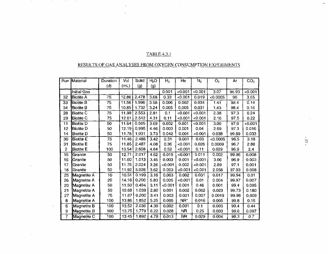
TABLE 4.3.1

RESULTS OF GAS ANALYSES FROM OXYGEN CONSUMPTION EXPERIMENTS

Run

3233342829111214303121516171825262021278697

Material

nitial GasBiotite ABiotite BBiotite BBiotite CBiotite CBiotite DBiotite DBiotite DBiotite EBiotite EBiotite EGraniteGraniteGraniteGraniteMagnetite AMagnetite AMagnetite AMagnetite AMagnetite AMagnetite AMagnetite BMagnetite BMagnetite C

Duration(d)

75757575755050507575100505050501020505075100100100100

Vol(mL)

12.8611.5610.8511.9912.6111.6412.1911.7811.4611.8513.5412.7111.6011.7511.9210.5114.1811.5010.6811.8713.8613.5213.7513.45

Solid

(9)

2.4781.9961.7322.5532.5120.5050.9951.0312.4882.4872.6082.0171.0132.0245.0260.1990.2000.4941.0390.2001.8522.0361.7791.892

H2O

(g)

3.683.583.242.814.313.694.463.733.424.084.844.623.453.263.623.165.833.112.803.415.254.396.224.79

H2

0.0010.330.0060.005

0.10.11

0.0020.0030.0420.310.360.520.0190.003<0.0010.0030.0030.005<0.0010.0010.0030.0050.0020.0280.013

He

<0.001<0.0010.0020.005<0.001<0.0010.0010.0010.0010.001

<0.001<0.001<0.0010.0010.002<0.0010.002

<0.0010.0010.0020.001NR*

0.001NRNR

N2

<0.0010.0190.0340.031<0.001<0.001<0.001

0.04<0.001

0.030.0260.110.011

<0.001<0.001<0.0010.0310.010.460.0620.0070.016

0.10.25

0.029

o2

3.07<0.0005

1.411.432.382.163.002.690.038

<0.00050.00090.0290.0023.062.892.0580.0170.0040.0010.0230.00190.0050.0030.0030.004

Ar

96.9396

98.498.497.397.597.097.399.8996.596.796.999.9696.997.197.9399.9499.9799.499.7399.9899.899.499.699.3

CO2

<0.0013.650.140.160.240.22

<0.0010.0160.0333.182.882.4

0.0080.0030.0010.0080.01

0.0070.0950.1800.0090.150.440.0970.7

KEY TO TABLE 4.3.1

All runs were in water at 100°C; run numbers indicate chronological sequence; missing numbers between I and 35 indicate failed runs, due toleaking vessels.

All biotite specimens prepared from Bancroft material

Biotite A = Untreated, -100 mesh fraction

Biotite B = Pre-leached (20 d, 150°C, 0.01 mol/L NaCl), -100 mesh fraction

Biotite C = Untreated, -40/+100 mesh fraction (ultrasonically cleaned)

Biotite D = Pre-leached (20 d, 150°C, 0.01 mol/L NaCl), -40/+100 mesh fraction (ultrasonically cleaned before leaching)

Biotite E = Re-ground, without ultrasonic cleaning or pre-leaching

Magnetite A = "Mapico Black", as received

Magnetite 8 = "Mapico Black", freshly reduced in CO/CO2 at 800°C

Magnetite C = Johnson-Matthey high-purity material

NR = Not Recorded

Granite was crushed and sieved to produce a +40/-60 mesh-size fraction, then pre-leached (20 d, 150°C, 0.01 mol/L NaCl)

NOTE: Runs 14 and 15 were with ultra-high-purity Ar starting gas

TABLE 4.3.2

CALCULATION OF AVERAGE OXYGEN CONSUMPTION RATES FROM GAS ANALYSES

Run

323334282911123031216171825262021278

Material

Biotite ABiotite BBiotite BBiotite CBiotite CBiotite DBiotite DBiotite EBiotite EBiotite EGranite **Granite **Granite **Magnetite AMagnetite AMagnetite AMagnetite AMagnetite AMagnetite A

MolO2

(gas)1.06E-059.26E-068.91 E-061.06E-059.45E-069.88E-069.38E-069.13E-068.78E-069.91 E-069.88E-069.84E-068.18E-069.29E-061.06E-051.05E-059.77E-061.07E-051.05E-05

MolO2

(aq)1.54E-071.50E-071.36E-071.18E-071.81E-071.55E-071.87E-071.43E-071.71E-072.03E-071.44E-071.37E-071.52E-071.33E-072.44E-071.30E-071.17E-071.43E-072.20E-07

MolO2

(total)1.07E-059.41 E-069.04E-061.07E-059.63E-061.00E-059.56E-069.27E-068.95E-061.01E-051.00E-059.98E-068.33E-069.42E-061.08E-051.07E-059.89E-061.08E-051.07E-05

MolO2

consumed1.07E-055.15E-064.89E-062.43E-062.89E-06

<10%1.22E-069.27E-068.95E-061.00E-05

<10%<10%

2.80E-069.37E-061.08E-051.07E-059.81 E-061.08E-051.07E-05

Time(s)

6.48E+066.48E+066.48E+066.48E+066.48E+064.32E+064.32E+066.48E+066.48E+068.64E+064.32E+064.32E+064.32E+068.64E+051.73E+064.32E+064.32E+066.48E+068.64E+06

Rate(mol/s)

1.66E-127.95E-137.55E-133.75E-134.47E-132.3E-132.81E-131.43E-121.38E-121.16E-122.32E-132.31E-136.49E-131.08E-116.25E-122.47E-122.27E-121.67E-121.24E-12

Ratemol/m2-s1.50E-138.91E-149.76E-145.78E-147.00E-141.81E-131.11E-131.03E-139.90E-147.92E-142.29E-131.14E-131.29E-136.19E-123.55E-125.68E-132.48E-139.48E-137.59E-14

Limit?*

LowerNoNoNoNo

UpperNo

LowerLowerLowerUpperUpper

NoLowerLowerLowerLowerLowerLower

For runs showing <10% O2 consumption, an upper limit of 10% is used in the calculation; for runs showing>90% O2 consumption, the resulting rate is regarded as a lower limit.For granite, a specific surface area of 1 m2/g is assumed.

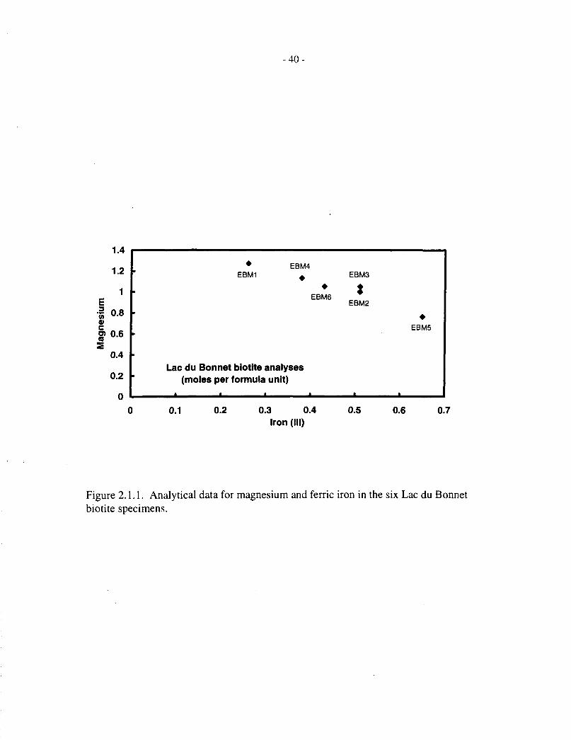
- 4 0 -

1.4

1.2

1

1 0.8a>§> 0.6(0

0.4

0.2

0

• EBM4EBM1 ^

•

Lac du Bonnet biotite analyses(moles per formula unit)

•EBM6

EBM3

tEBM2

ft

•EBM5

ft

0.1 0.2 0.3 0.4Iron (III)

0.5 0.6 0.7

Figure 2.1.1. Analytical data for magnesium and ferric iron in the six Lac du Bonnetbiotite specimens.

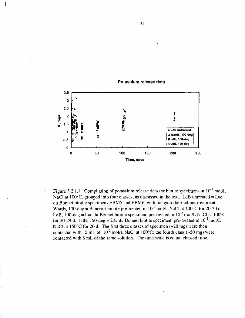
-41 -

Potassium release data

3.5 r

X• LdB untreatedQWards, 100-deg• LdB, 100-degxLdB, 150-deg

50 100 150

Time, days

200 250

Figure 3.2.1.1. Compilation of potassium release data for biotite specimens in 10"2 mol/LNaCl at 100°C, grouped into four classes, as discussed in the text. LdB untreated = Lacdu Bonnet biotite specimens EBM5 and EBM6, with no hydrothermal pre-treatment.Wards, 100-deg = Bancroft biotite pre-treated in 10'2 mol/L NaCl at 100°C for 20-30 d.LdB, 100-deg = Lac du Bonnet biotite specimen, pre-treated in 10~2 mol/L NaCl at 100°Cfor 20-29 d. LdB, 150-deg = Lac du Bonnet biotite specimen, pre-treated in 10" mol/LNaCl at 150°C for 20 d. The first three classes of specimen (-20 mg) were thencontacted with 15 mL of 10'2 mol/L NaCl at 100°C; the fourth class (-50 mg) werecontacted with 8 mL of the same solution. The time scale is actual elapsed time.

- 4 2 -

Mg, EBM5, no pre-leach

50 100 150

Time (days)

200 250

Figure 3.2.2.1. Magnesium release data for untreated Lac du Bonnet biotite, specimenEBM5, ~20-mg samples contacted with 15 mL (initial volume) of 10"2 mol/L NaCl at100°C. The time scale represents effective time at constant volume of 15 mL and biotitemass of 20.0 mg.

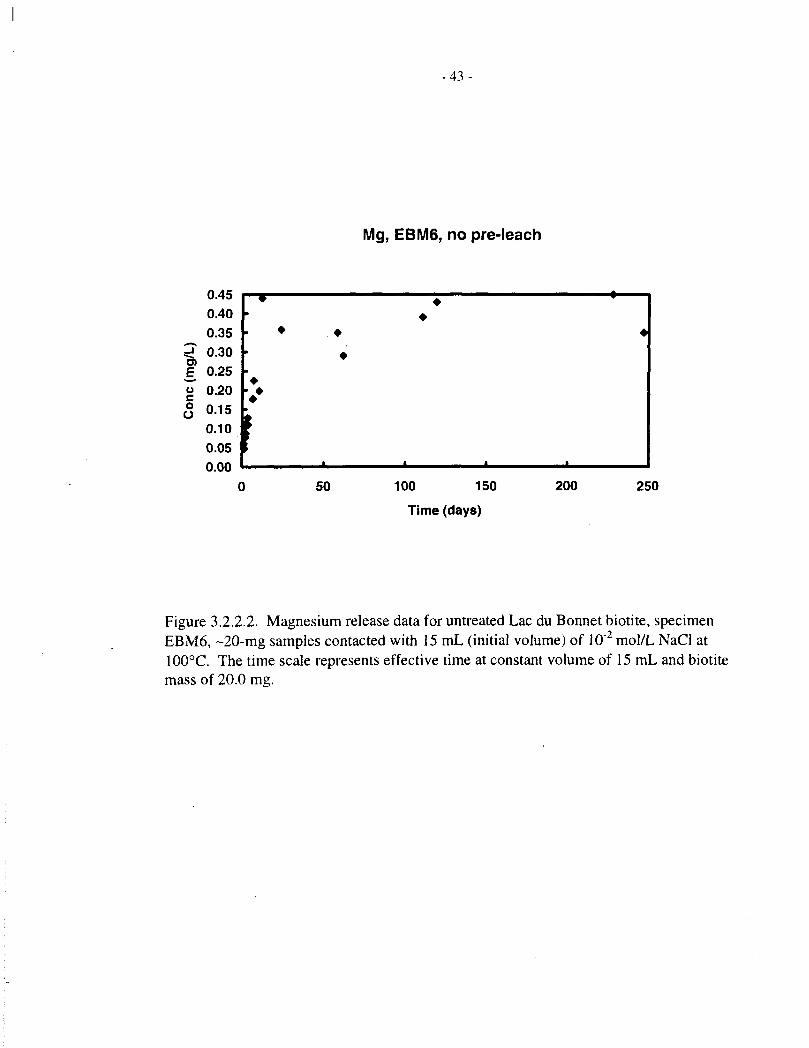
- 4 3 -

Mg, EBM6, no pre-leach

•

•

50 100 150

Time (days)

200 250

Figure 3.2.2.2. Magnesium release data for untreated Lac du Bonnet biotite, specimenEBM6, ~20-mg samples contacted with 15 mL (initial volume) of 10~2 mol/L NaCl at100°C. The time scale represents effective time at constant volume of 15 mL and biotitemass of 20.0 mg.

- 4 4 -

Mg, EBM5, pre-leached

0.0 20.0 40.0 60.0 80.0

Time (days)

100.0 120.0 140.0

Figure 3.2.2.3. Magnesium release data for Lac du Bonnet biotite, specimen EBM5,~20-mg samples, pre-treated with 102 mol/L NaCl at 100°C for 20 or 29 days (see inset),then contacted with 15 mL (initial volume) of 10'2 mol/L NaCl at 100°C. The time scalerepresents effective time at constant volume of 15 mL and biotite mass of 20.0 mg.

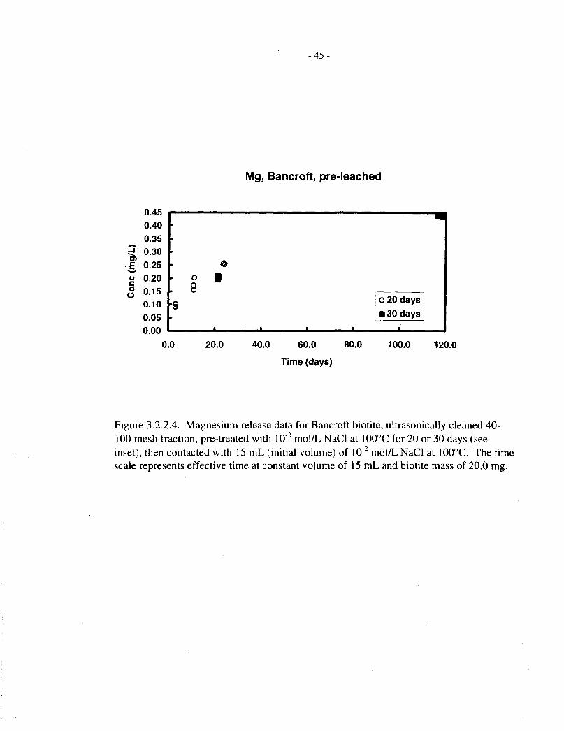
-45 -

Mg, Bancroft, pre-leached

oou

0.450.400.350.300.250.200.150.100.050.00

0.0

o8

20.0

•

40.0 60.0

Time (days)

80.0

o 20 days

• 30 days

100.0 120.0

Figure 3.2.2.4. Magnesium release data for Bancroft biotite, ultrasonically cleaned 40-100 mesh fraction, pre-treated with 10~2 mol/L NaCl at 100°C for 20 or 30 days (seeinset), then contacted with 15 mL (initial volume) of 10"2 mol/L NaCl at 100°C. The timescale represents effective time at constant volume of 15 mL and biotite mass of 20.0 mg.

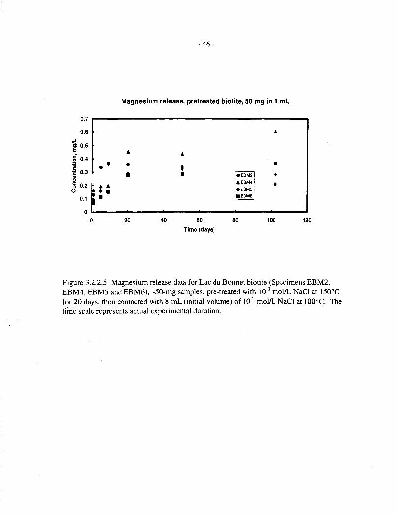
-46-

0.7

0.6

|> 0.5

o 0.4

| 0.3

Sg 0.2o

0.1

0

Magnesium release, pretreated biotite, 50 mg in 8 mL

*• A

• # * •

i • • EBM2

AEBM4

• EBM5

• EBM6

I

A

m

:

•

20 40 60

Time (days)

80 100 120

Figure 3.2.2.5 Magnesium release data for Lac du Bonnet biotite (Specimens EBM2,EBM4, EBM5 and EBM6), -50-mg samples, pre-treated with 10"2 mol/L NaCl at 150°Cfor 20 days, then contacted with 8 mL (initial volume) of 10"2 mol/L NaCl at 100°C. Thetime scale represents actual experimental duration.

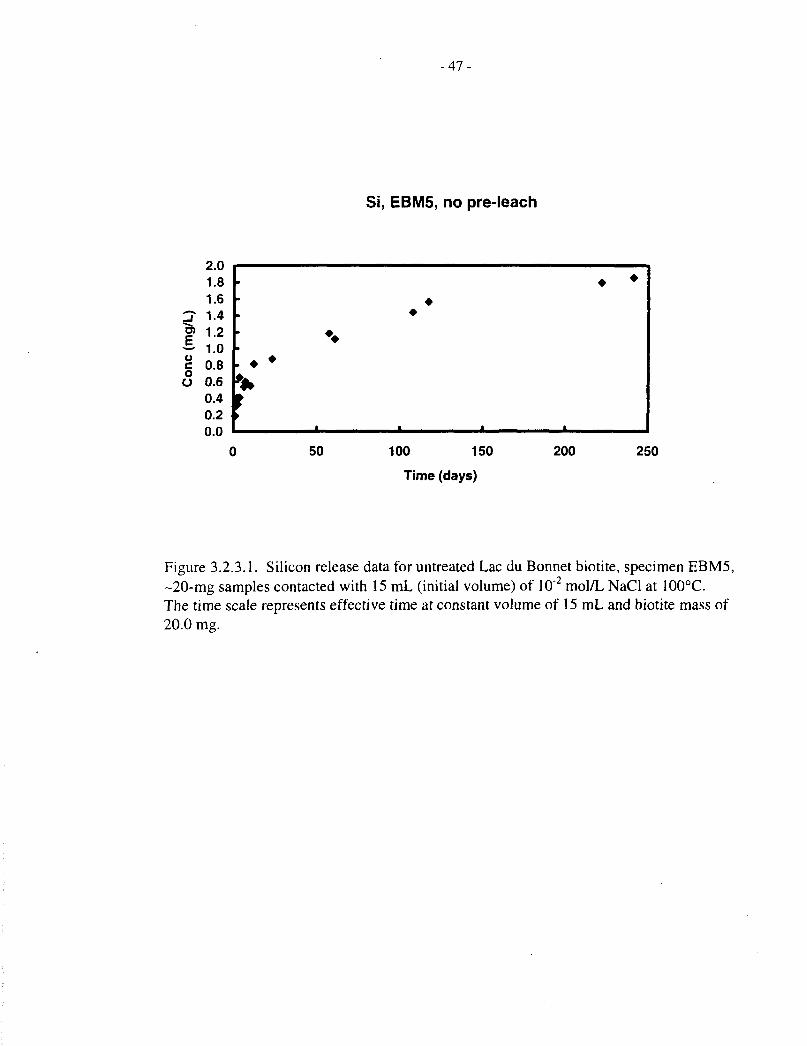
- 4 7 -

Si, EBM5, no pre-leach

ugo

2.01.81.61.41.21.00.80.60.40.20.0

• •

50 100 150

Time (days)

200 250

Figure 3.2.3.1. Silicon release data for untreated Lac du Bonnet biotite, specimen EBM5,~20-mg samples contacted with 15 mL (initial volume) of 10"2 mol/L NaCl at 100°C.The time scale represents effective time at constant volume of 15 mL and biotite mass of20.0 mg.

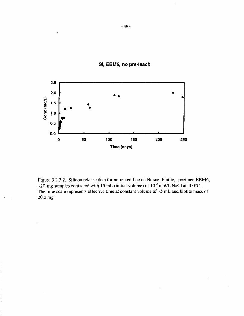
-48 -

Si, EBM6, no pre-leach

• ••

50 100 150

Time (days)

200 250

Figure 3.2.3.2. Silicon release data for untreated Lac du Bonnet biotite, specimen EBM6,~20-mg samples contacted with 15 mL (initial volume) of 10"2 mol/L NaCl at 100°C.The time scale represents effective time at constant volume of 15 mL and biotite mass of20.0 mg.

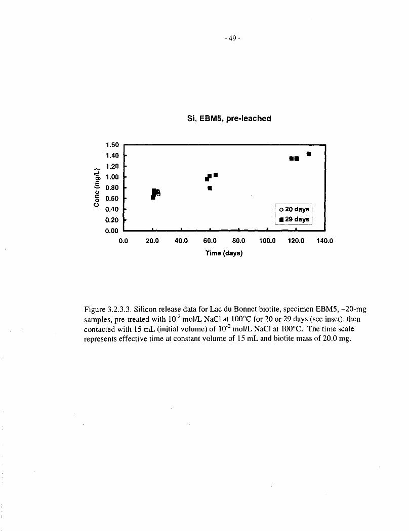
-49-

Si, EBM5, pre-leached

"a.uou

1.60

1.40

1.20

1.00

0.80

0.60

0.40

0.20

0.00

1 * •

• 1 • • I

. . -

o 20 days

• 29 days•

0.0 20.0 40.0 60.0 80.0

Time (days)

100.0 120.0 140.0

Figure 3.2.3.3. Silicon release data for Lac du Bonnet biotite, specimen EBM5, ~20-mgsamples, pre-treated with 10~2 mol/L NaCl at 100°C for 20 or 29 days (see inset), thencontacted with 15 mL (initial volume) of 10~2 mol/L NaCl at 100°C. The time scalerepresents effective time at constant volume of 15 mL and biotite mass of 20.0 mg.

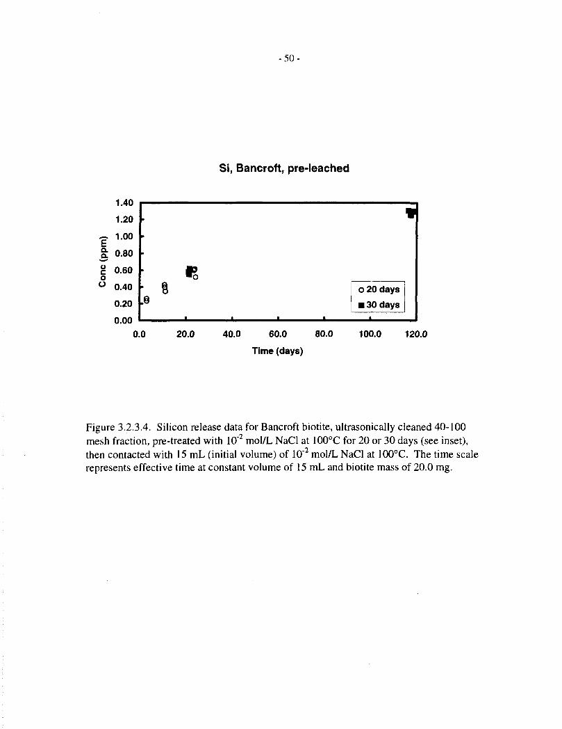
- 5 0 -

Si, Bancroft, pre-leached

1.4U

1.20

~ 1.00

§: o.8o

g 0.60o° 0.40

0.20

n nn

•

•

•

.§

• • • i

V

o 20 days

• 30 days•

0.0 20.0 40.0 60.0 80.0Time (days)

100.0 120.0

Figure 3.2.3.4. Silicon release data for Bancroft biotite, ultrasonically cleaned 40-100mesh fraction, pre-treated with 10'2 mol/L NaCl at 100°C for 20 or 30 days (see inset),then contacted with 15 mL (initial volume) of 10"2 mol/L NaCl at 100°C. The time scalerepresents effective time at constant volume of 15 mL and biotite mass of 20.0 mg.

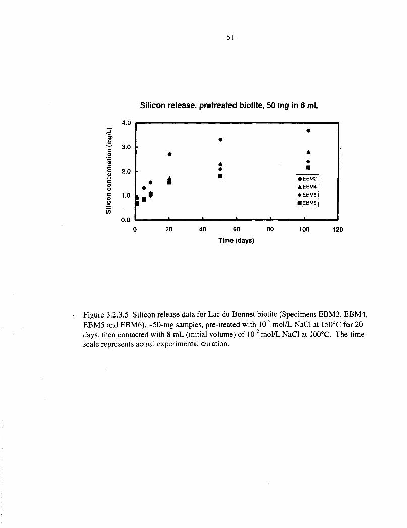
-51 -

Silicon release, pretreated biotite, 50 mg in 8 mL

o

4.0

3.0

•

• EBM2AEBM4• EBM5• EBM6

20 40 60 80

Time (days)

100 120

Figure 3.2.3.5 Silicon release data for Lac du Bonnet biotite (Specimens EBM2, EBM4,EBM5 and EBM6), -50-mg samples, pre-treated with 10~2 mol/L NaCl at 150°C for 20days, then contacted with 8 mL (initial volume) of 10"2 mol/L NaCl at 100°C. The timescale represents actual experimental duration.

- 5 2 -

Fractional release, untreated EBM5

50 100 150

Effective time (days)

200 250

Figure 3.2.4.1. Magnesium and silicon release data for untreated Lac du Bonnet biotite,Specimen EBM5 (see Figures 3.2.2.1 and 3.2.3.1), expressed as fractional release ofmagnesium and silicon.

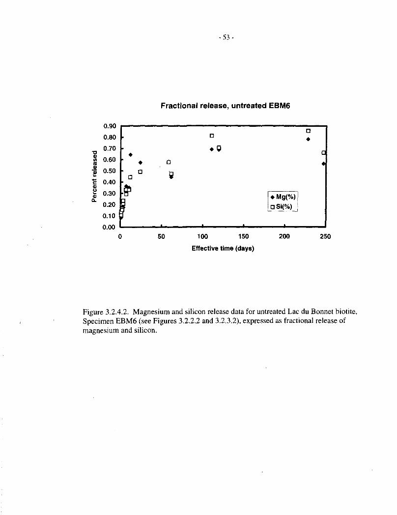
-53-

Fractional release, untreated EBM6as

edre

le

4-*

ilk

Per

ct

0.90

0.80

0.70

0.60

0.50

0.40

0.30

0.20

0.1a

0.00

•

•

a

•i

•a

a

9

•• Q

* *

• Mg(%)

a Si(%)

•

D•

C

•

50 100 150

Effective time (days)

200 250

Figure 3.2.4.2. Magnesium and silicon release data for untreated Lac du Bonnet biotite,Specimen EBM6 (see Figures 3.2.2.2 and 3.2.3.2), expressed as fractional release ofmagnesium and silicon.

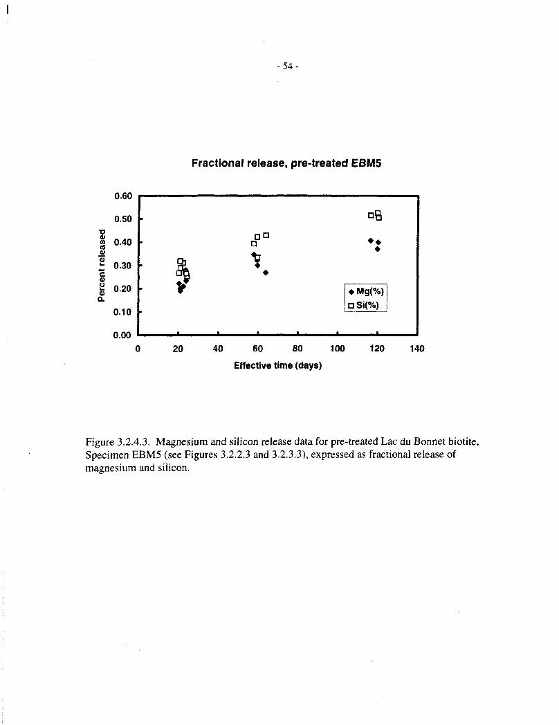
- 5 4 -

Fractional release, pre-treated EBM5

0.60

0.50-aw 0.40to

£ 0.30c0)

jj 0.20a.

0.10

0.00

*

•

• > • * •

•

• Mg(%)

20 40 60 80 100 120 140

Effective time (days)

Figure 3.2.4.3. Magnesium and silicon release data for pre-treated Lac du Bonnet biotite,Specimen EBM5 (see Figures 3.2.2.3 and 3.2.3.3), expressed as fractional release ofmagnesium and silicon.

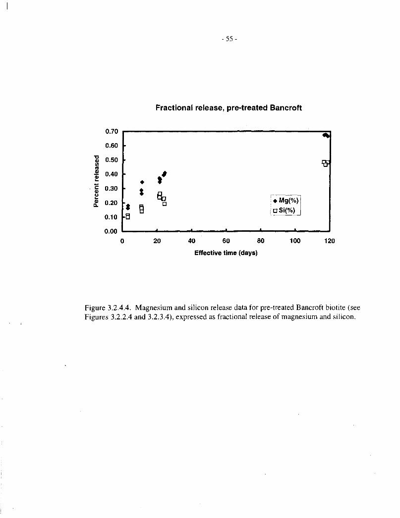
- 55 -

Fractional release, pre-treated Bancroft

"S 0.50<flto

I 0.40

20 40 60 80

Effective time (days)

100 120

Figure 3.2.4.4. Magnesium and silicon release data for pre-treated Bancroft biotite (seeFigures 3.2.2.4 and 3.2.3.4), expressed as fractional release of magnesium and silicon.

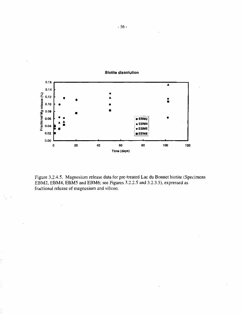
- 5 6 -

Biotite dissolution

0.16

0.14

8 0.10

S> 0.08

c 0.06o

I 0.04

0.02

0.00

••

• •

» •1

• EBM2

AEBM4

• EBM5

• EBM6

A

••

•

•

20 40 60

Time (days)

80 100 120

Figure 3.2.4.5. Magnesium release data for pre-treated Lac du Bonnet biotite (SpecimensEBM2, EBM4, EBM5 and EBM6; see Figures 3.2.2.5 and 3.2.3.5), expressed asfractional release of magnesium and silicon.

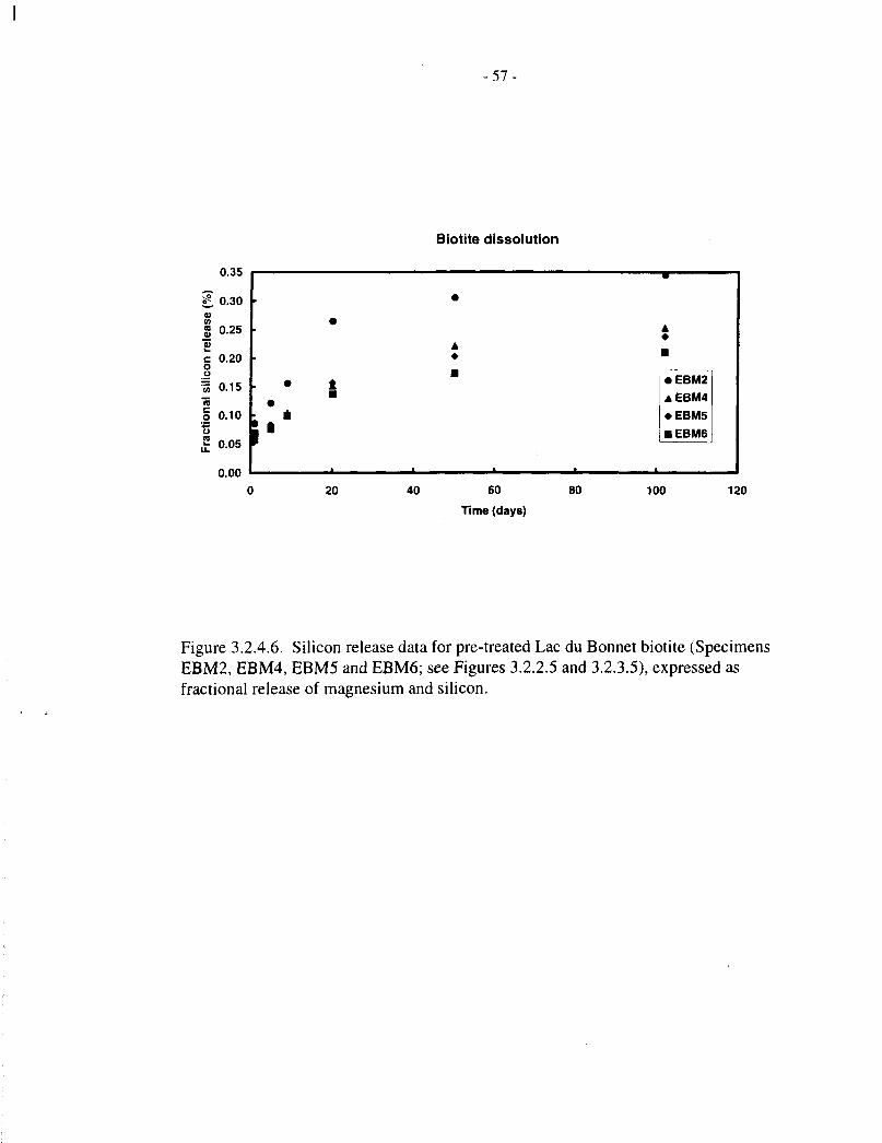
- 5 7 -

Biotite dissolution

0.35

£ 0.30

g 0.252c 0.20ooI 0.15no 0.10.? 0.05

0.00

1

••

•

t

•

•

•

•

• EBM2AEBM4

• EBM5

• EBM6

20 40 60

Time (days)

80 100 120

Figure 3.2.4.6. Silicon release data for pre-treated Lac du Bonnet biotite (SpecimensEBM2, EBM4, EBM5 and EBM6; see Figures 3.2.2.5 and 3.2.3.5), expressed asfractional release of magnesium and silicon.

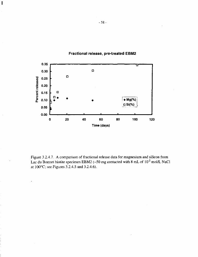
-58 -

Fractional release, pre-treated EBM2

0.35

0.30

•g 0.25

•3 0.20

| 0.15o

£ 0.10

0.05

0.00

*

•

a

•

A • * •

LI

• Mg(%)

a Si(%)

•

20 40 60 80 100

Time (days)

120

Figure 3.2.4.7. A comparison of fractional release data for magnesium and silicon fromLac du Bonnet biotite specimen EBM2 (-50 mg contacted with 8 mL of 10"2 mol/L NaClat !00°C; see Figures 3.2.4.5 and 3.2.4.6).

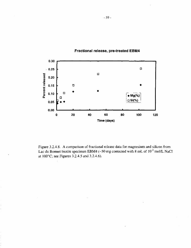
-59 -

Fractional release, pre-treated EBM4

0.30

. 0.25

;ase

d

8

Per

cer

0.20

0.15

0.10

0.05

0.00

aa

? • •

a

•

a

•

•

•

|*Mg(%)

• Si(%)

20 40 60 80 100

Time (days)

120

Figure 3.2.4.8. A comparison of fractional release data for magnesium and silicon fromLac du Bonnet biotite specimen EBM4 (-50 mg contacted with 8 mL of 10"2 mol/L NaClat l00°C; see Figures 3.2.4.5 and 3.2.4.6).

-60-

Fractional release, pre-treated EBM5

0.25

0.20

8 0.15£

§ 0.10

0.05

0.00

•

•a

3 • •

a

•

D

• • •

a

•

• Mg(%)

20 40 60

Time (days)

80 100 120

Figure 3.2.4.9. A comparison of fractional release data for magnesium and silicon fromLac du Bonnet biotite specimen EBM5 (-50 mg contacted with 8 mL of 10 2 mol/L NaClat 100°C; see Figures 3.2.4.5 and 3.2.4.6).

-61 -

Percentage release, pre-treated EBM6

0.25

20 40 60

Time (days)

80 100 120

Figure 3.2.4.10. A comparison of fractional release data for magnesium and silicon fromLac du Bonnet biotite specimen EBM6 (-50 mg contacted with 8 mL of 10"2 mol/L NaClat 100°C; see Figures 3.2.4.5 and 3.2.4.6).

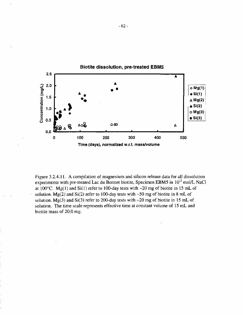
- 6 2 -

Biotite dissolution, pre-treated EBM5

oMg(1)

• Si(1)

A Mg(2)

• Si(2)

o Mg(3)

• Si(3)

100 200 300 400

Time (days), normalized w.r.t. mass/volume

500

Figure 3.2.4.11. A compilation of magnesium and silicon release data for all dissolutionexperiments with pre-treated Lac du Bonnet biotite, Specimen EBM5 in 10~2 mol/L NaClat 100°C. Mg(l) and Si(l) refer to 100-day tests with -20 mg of biotite in 15 mL ofsolution. Mg(2) and Si(2) refer to 100-day tests with -50 mg of biotite in 8 mL ofsolution. Mg(3) and Si(3) refer to 200-day tests with -20 mg of biotite in 15 mL ofsolution. The time scale represents effective time at constant volume of 15 mL andbiotite mass of 20.0 mg.

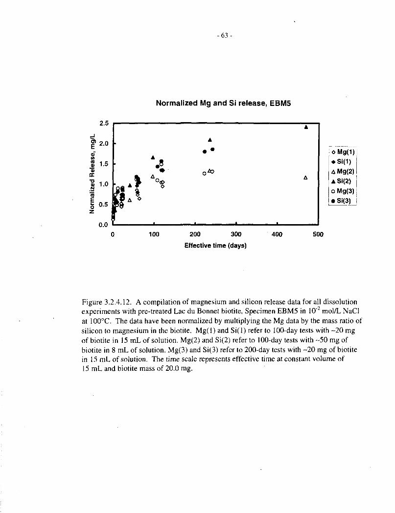
- 6 3 -

Normalized Mg and Si release, EBM5

o> A

oMg(1)

• Si(1)

A Mg(2)

ASi(2)

o Mg(3)

• Si(3)

100 200 300

Effective time (days)

400 500

Figure 3.2.4.12. A compilation of magnesium and silicon release data for all dissolutionexperiments with pre-treated Lac du Bonnet biotite, Specimen EBM5 in 10" mol/L NaClat 100°C. The data have been normalized by multiplying the Mg data by the mass ratio ofsilicon to magnesium in the biotite. Mg(l) and Si(l) refer to 100-day tests with -20 mgof biotite in 15 mL of solution. Mg(2) and Si(2) refer to 100-day tests with -50 mg ofbiotite in 8 mL of solution. Mg(3) and Si(3) refer to 200-day tests with -20 mg of biotitein 15 mL of solution. The time scale represents effective time at constant volume of15 mL and biotite mass of 20.0 mg.

-64 -

Basal surface exposed by"raggedness", i.e., imperfectregistry between lamellae

Edge surface exposedby basal roughness

Edge surface increasedby jaggedness

FIGURE 3.2.5.1 Schematic sketch of a biotite flake, with terraced structure exaggeratedto illustrate the relationship between surface roughness and edge and basal surface areas.

-65-

1SKU 1.60KX 6.25H 0813

FIGURE 3.2.5.2 Scanning electron micrograph of a biotite flakes, showing the actualterraced structure of (a) Bancroft biotite (micrograph #0813) and (b) Lac du Bonnetbiotite (micrograph # 0827). In both cases, the terraced structure is slightly enhanced bydissolution, after contact with 0.01 mol/L NaCl at pH 11 for 20 d at 200°C (see Taylorand Owen 1995).

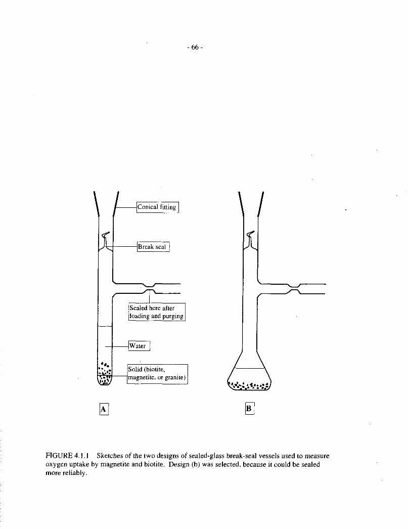
- 6 6 -

Conical fitting

Break seal

Sealed here afterloading and purging

Water

Solid (biotite,magnetite, or granite)

FIGURE 4.1.1 Sketches of the two designs of sealed-glass break-seal vessels used to measureoxygen uptake by magnetite and biotite. Design (b) was selected, because it could be sealedmore reliably.

AECL-11571COG-96-157-1

Cat. No. / N° de cat.: CC2-11571EISBN 0-660-16965-7

ISSN 0067-0367

To identify individual documents in the series, we have assigned an AECL- number to each.Please refer to the AECL- number when requesting additional copies of this document from

Scientific Document Distribution Office (SDDO)AECLChalk River, OntarioCanada K0J 1J0

Fax:(613)584-1745 Tel.: (613) 584-3311ext. 4623

Price: B

Pour identifier les rapports individuels faisant partie de cette serie, nous avons affecte unnumero AECL- a chacun d'eux. Veuillez indiquer le numero AECL- lorsque vous demandezd'autres exemplaires de ce rapport au

Service de Distribution des documents officiels (SDDO)EACLChalk River (Ontario)Canada K0J 1J0

Fax:(613)584-1745 Tel.: (613) 584-3311poste 4623

Prix: B

Copyright © Atomic Energy of Canada Limited, 1997.Printed on recycled paper with vegetable-oil-based inks