Petroleum Fractions Liquid – Vapor Equilibrium Simulation using Unisim Design C.pdf 11 15.pdf · · 2015-11-11Petroleum Fractions Liquid – Vapor Equilibrium Simulation using

REV. CHIM. (Bucharest) ♦ 66 ♦ No. 11 ♦ 2015 http://www.revistadechimie.ro 1867

Petroleum Fractions Liquid – Vapor EquilibriumSimulation using Unisim Design®

CRISTIAN PATRASCIOIU1*, GRIGORE STAMATESCU2

1 Petroleum-Gas University of Ploiesti, Automatic Control, Computers and Electronics Department, 39 Bucuresti Blvd., 100680,Ploiesti, Romania2 University Politehnica of Bucharest, Automatic Control and Industrial Informatics Department, 313 Splaiul Independentei,060042, Bucharest, Romania

The Unisim® environment represents a valuable tool applied for chemical process simulation and automaticcontrol systems associated to such processes. Due to the specific nature of petroleum products, instead ofpure chemical components the simulator operates with pseudocomponents, with different configurationprocedures for each case. If the operation for the first case is well known to the smallest detail, configuringthe simulator being straight forward, the second case is more complex and the configuration is carried out byspecific operations. The paper describes research carried out in two directions. For the first one, the necessarystages for the usage of pseudocomponents in the computation of liquid-vapor equilibrium. The second stageis represented by the identification and testing of the Unisim® configuration operations for cases in whichpetroleum products are involved. Three representative cases were analyzed: petroleum, diesel and petroleum– water mixture.

Keywords: Unisim®, chemical process simulation, petroleum products, pseudocomponents

The simulation of chemical processes, especially thatof refiery processes and installations, requires as acompulsory step the computation of the liquid – vaporequilibrium, in both transport pipelines, hydraulicresistances, separator vessels as well in fractioningcolumns. The simulation of chemical processes is possibleif numerical sumelators ar used, such as HYSYS, Unisim®

and PRO II, each of these solutions including specializedmodules for the computation of the liquid – vaporequilibrium of petroleum products.

In the case of the classical usage of the Unisim®

simulator, the computation of the liquid – vapor equilibriumis conditioned by following three configuration steps [1]:

- selecting the chemical components from the simulatordatabase;

- selecting the thermodynamic model of the liquid –vapor equilibrium;

- defining the concentrations associated to eachchemical component.

This technique is applied only to processes which involvepure chemical components. For exemple, in the case ofbinary fractioning, the HYSYS simulator was used for staticand dynamic simulation fo the fractioning process [2, 3].

Most of the processes in refineries operate withpetroleum products, including oil. In these cases theUnisim® simulator will operate with pseudocomponentsinstead of chemical components [4-6]. The research carriedout by the authors indicated the fact that switching fromchemical components whose physical properties areincluded in the simulator database, to pseudocomponents,involves the following stages:

- defining the properties of the petroleum product (PRFdistillation curve, STAS distillation curve, averageproperties);

- generating pseudocomponents in the range of boilingtemperatures for the petroleum product;

- selection of pseudocomponents which define adistillation curve as close as possible to the experimentalone;

- computing the optimal concentration for each selectedpseudocomponent such that both the distillation curve andthe average properties are as close as possible to theexperimental ones.

This new approach for the usage patterns of the Unisim®

simulator requires following different configuration stepsof the environment. The paper covers the actual simulatorconfiguration procedure for three fundamental petroleumproducts:

a) oil;b) petroleum product (gasoline, diesel);c) oil – water mixture.For each of these options, both the configuration

particularities of the Unisim® simulator and an applicationfor liquid – vapor equilibrium computation are presented.

Particularities in defining the component list for oilThis case is specific to a petroleum product without

being accompanied by pure chemical components. Crudeoil belongs to this category. The simulation of liquid – vaporequilibrium requires following the listed steps:

a) selecting the thermodynamic model used bypetroleum products;

b) analysis of the petroleum product;c) introducing in the simulator of the laboratory analysis

characteristics of the petroleum product;d) computing the pseudocomponents;e) defining the simulation window Case main;f) simulation of the liquid – vapor equilibrium.

Selecting the thermodynamic modelFor petroleum products, the usage of the Peng –

Robinson thermodynamic model is reccomended. This

* email: [email protected]; Tel.: (+40) 0244573171

http://www.revistadechimie.ro REV. CHIM. (Bucharest) ♦ 66 ♦ No. 11 ♦ 20151868

model is based on the state equation with the same name,developed in 1976 and respects the following requirements[7, 8]:

a) the equation parameters should be expressed basedon the critical properties and the acentric factor of thechemical components;

b) the model should correctly predict the properties inranges around the critical point;

c) the mixing rules only concern binary mixtures, beingtemperature and pressure independent;

d) the state equation can be applied to the computationof the hydrocarbon mixture properties.

In the Unisim Design® simulation environment theselection of the thermodynamic model is performed withthe help of the command menu Current Fluid Package,where the Add command is used to insert the Peng –Robinson thermodynamic model.

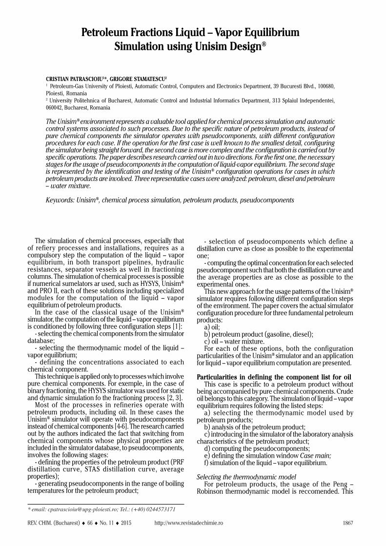
Analysis of the petroleum productThe petroleum product corresponding to this category

is oil which supplied an atmospheric distillation column.The laboratory data associated to the TBP curve are listedin Table 1 [9]. These analyses contain both the TBPdistillation curve as well as the average percentage –density curve.

Inserting the laboratory analyses data of the petroleumproduct

In order to insert the data resulting from the laboratoryanalysis in the Unisim Design® simulation environment,the following steps have to be carried out:

a) the Fluid Package window is minimized and we returnto the Simulation Basis Manager;

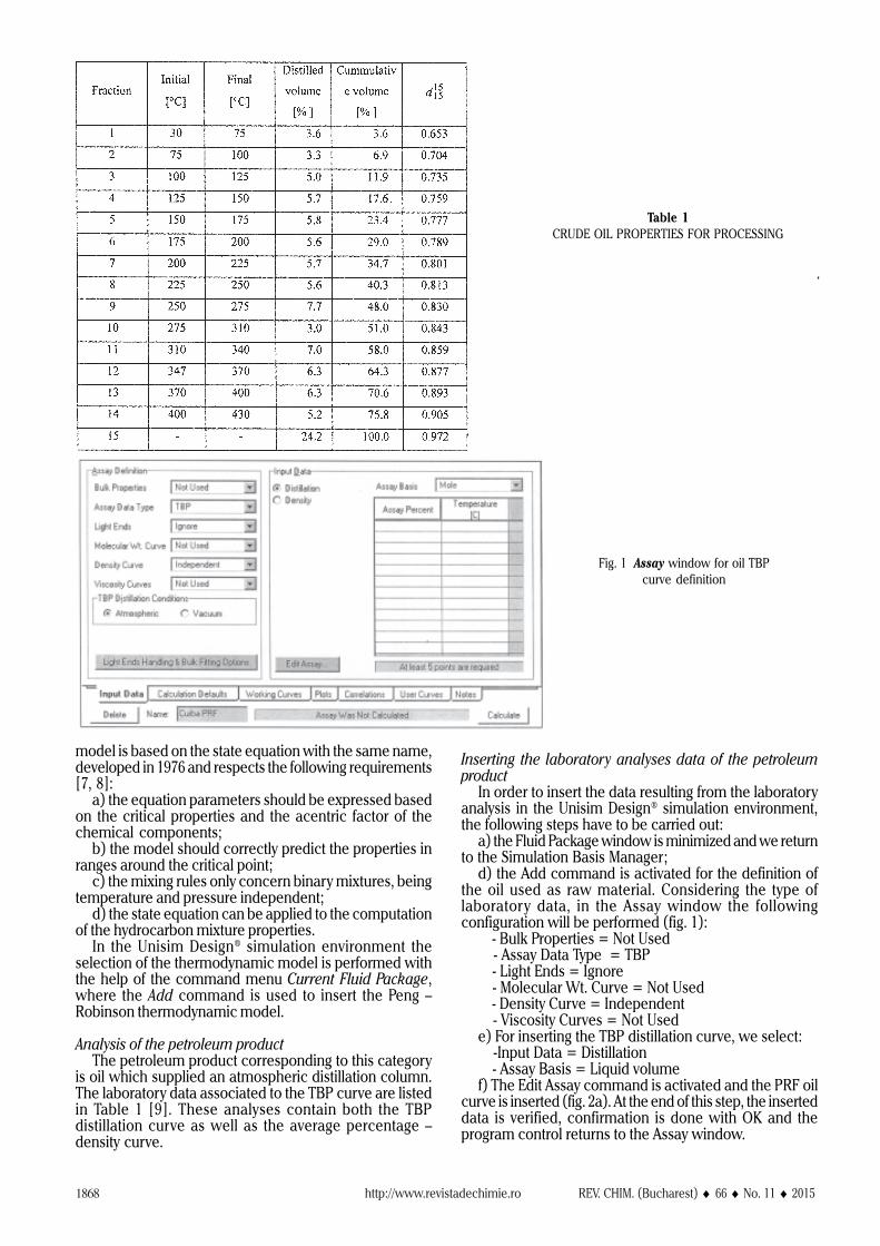
d) the Add command is activated for the definition ofthe oil used as raw material. Considering the type oflaboratory data, in the Assay window the followingconfiguration will be performed (fig. 1):

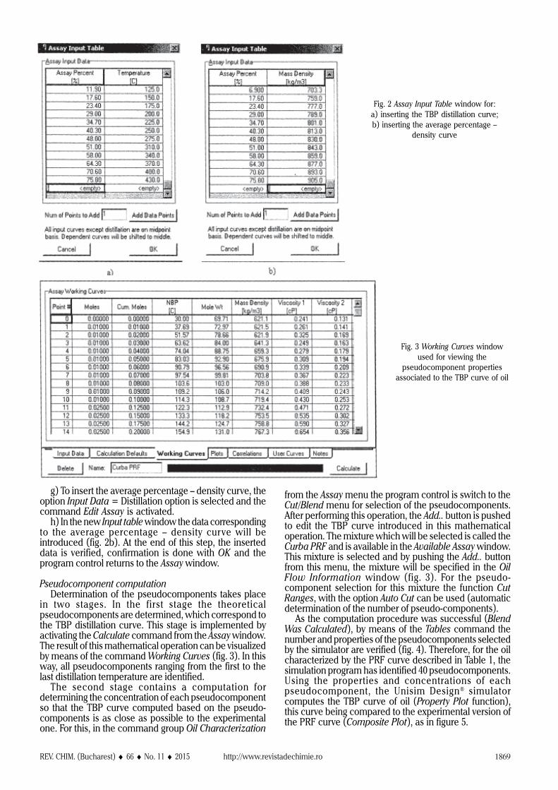
- Bulk Properties = Not Used - Assay Data Type = TBP - Light Ends = Ignore - Molecular Wt. Curve = Not Used - Density Curve = Independent - Viscosity Curves = Not Usede) For inserting the TBP distillation curve, we select: -Input Data = Distillation - Assay Basis = Liquid volumef) The Edit Assay command is activated and the PRF oil

curve is inserted (fig. 2a). At the end of this step, the inserteddata is verified, confirmation is done with OK and theprogram control returns to the Assay window.

Table 1CRUDE OIL PROPERTIES FOR PROCESSING

Fig. 1 Assay window for oil TBPcurve definition


g) To insert the average percentage – density curve, theoption Input Data = Distillation option is selected and thecommand Edit Assay is activated.

h) In the new Input table window the data correspondingto the average percentage – density curve will beintroduced (fig. 2b). At the end of this step, the inserteddata is verified, confirmation is done with OK and theprogram control returns to the Assay window.

Pseudocomponent computationDetermination of the pseudocomponents takes place

in two stages. In the first stage the theoreticalpseudocomponents are determined, which correspond tothe TBP distillation curve. This stage is implemented byactivating the Calculate command from the Assay window.The result of this mathematical operation can be visualizedby means of the command Working Curves (fig. 3). In thisway, all pseudocomponents ranging from the first to thelast distillation temperature are identified.

The second stage contains a computation fordetermining the concentration of each pseudocomponentso that the TBP curve computed based on the pseudo-components is as close as possible to the experimentalone. For this, in the command group Oil Characterization

from the Assay menu the program control is switch to theCut/Blend menu for selection of the pseudocomponents.After performing this operation, the Add.. button is pushedto edit the TBP curve introduced in this mathematicaloperation. The mixture which will be selected is called theCurba PRF and is available in the Available Assay window.This mixture is selected and by pushing the Add.. buttonfrom this menu, the mixture will be specified in the OilFlow Information window (fig. 3). For the pseudo-component selection for this mixture the function CutRanges, with the option Auto Cut can be used (automaticdetermination of the number of pseudo-components).

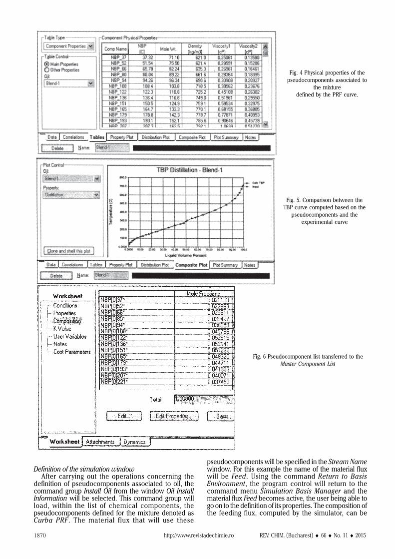
As the computation procedure was successful (BlendWas Calculated), by means of the Tables command thenumber and properties of the pseudocomponents selectedby the simulator are verified (fig. 4). Therefore, for the oilcharacterized by the PRF curve described in Table 1, thesimulation program has identified 40 pseudocomponents.Using the properties and concentrations of eachpseudocomponent, the Unisim Design® simulatorcomputes the TBP curve of oil (Property Plot function),this curve being compared to the experimental version ofthe PRF curve (Composite Plot), as in figure 5.

Fig. 2 Assay Input Table window for:a) inserting the TBP distillation curve;b) inserting the average percentage –

density curve

Fig. 3 Working Curves windowused for viewing the

pseudocomponent propertiesassociated to the TBP curve of oil


Definition of the simulation windowAfter carrying out the operations concerning the

definition of pseudocomponents associated to oil, thecommand group Install Oil from the window Oil InstallInformation will be selected. This command group willload, within the list of chemical components, thepseudocomponents defined for the mixture denoted asCurba PRF. The material flux that will use these

pseudocomponents will be specified in the Stream Namewindow. For this example the name of the material fluxwill be Feed. Using the command Return to BasisEnvironment, the program control will return to thecommand menu Simulation Basis Manager and thematerial flux Feed becomes active, the user being able togo on to the definition of its properties. The composition ofthe feeding flux, computed by the simulator, can be

Fig. 4 Physical properties of thepseudocomponents associated to

the mixturedefined by the PRF curve.

Fig. 5. Comparison between theTBP curve computed based on the

pseudocomponents and theexperimental curve

Fig. 6 Pseudocomponent list transferred to theMaster Component List


visualized through the command Composition from theWorksheet, window (fig. 6).

Simulation of the liquid – vapor equilibrium for oilBy means of the newly created program a simulation

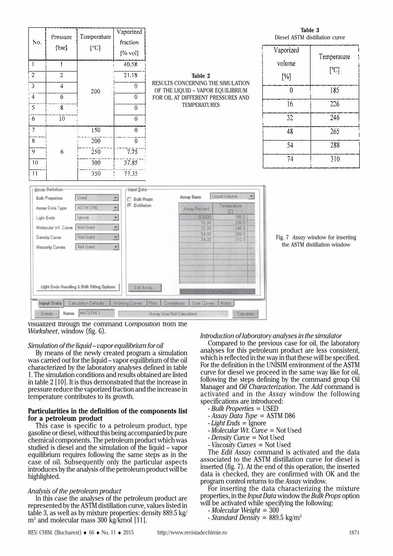
was carried out for the liquid – vapor equilibrium of the oilcharacterized by the laboratory analyses defined in table1. The simulation conditions and results obtained are listedin table 2 [10]. It is thus demonstrated that the increase inpressure reduce the vaporized fraction and the increase intemperature contributes to its growth.

Particularities in the definition of the components listfor a petroleum product

This case is specific to a petroleum product, typegasoline or diesel, without this being accompanied by purechemical components. The petroleum product which wasstudied is diesel and the simulation of the liquid – vaporequilibrium requires following the same steps as in thecase of oil. Subsequently only the particular aspectsintroduces by the analysis of the petroleum product will behighlighted.

Analysis of the petroleum productIn this case the analyses of the petroleum product are

represented by the ASTM distillation curve, values listed intable 3, as well as by mixture properties: density 889.5 kg/m3 and molecular mass 300 kg/kmol [11].

Introduction of laboratory analyses in the simulatorCompared to the previous case for oil, the laboratory

analyses for this petroleum product are less consistent,which is reflected in the way in that these will be specified.For the definition in the UNISIM environment of the ASTMcurve for diesel we proceed in the same way like for oil,following the steps defining by the command group OilManager and Oil Characterization. The Add command isactivated and in the Assay window the followingspecifications are introduced:

- Bulk Properties = USED- Assay Data Type = ASTM D86- Light Ends = Ignore- Molecular Wt. Curve = Not Used- Density Curve = Not Used- Viscosity Curves = Not UsedThe Edit Assay command is activated and the data

associated to the ASTM distillation curve for diesel isinserted (fig. 7). At the end of this operation, the inserteddata is checked, they are confirmed with OK and theprogram control returns to the Assay window.

For inserting the data characterizing the mixtureproperties, in the Input Data window the Bulk Props optionwill be activated while specifying the following:

- Molecular Weight = 300- Standard Density = 889.5 kg/m3

Table 2RESULTS CONCERNING THE SIMULATIONOF THE LIQUID – VAPOR EQUILIBRIUM

FOR OIL AT DIFFERENT PRESSURES ANDTEMPERATURES

Table 3Diesel ASTM distillation curve

Fig. 7 Assay window for insertingthe ASTM distillation window


Computation of the pseudocomponentsComputing of the pseudocomponents associated to the

petroleum product is carried out in the same manner asfor oil, that is:

a) The Calculate command from the Assay window isactivated, thus identifying all pseudocomponents betweenthe first and last distillation temperature.

b) In the command group Oil Characterization from theAssay menu the control of the program is switched to theCut/Blend menu for selecting the pseudocomponents andthe Add.. command is activated to link-edit the TBP curveto this mathematical operation. The mixture to be selectedis called PRF Curve and can be found in the Available Assaywindow.

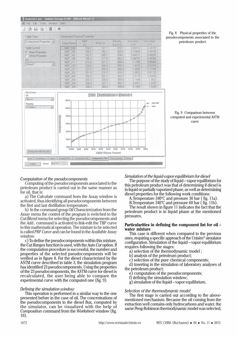
c) To define the pseudocomponents within this mixture,the Cut Ranges function is used, with the Auto Cut option. Ifthe computation procedure is successful, the number andproperties of the selected pseudocomponents will beverified as in figure 8. For the diesel characterized by theASTM curve described in table 3, the simulation programhas identified 23 pseudocomponents. Using the propertiesof the 23 pseudocomponents, the ASTM curve for diesel isrecalculated, the user being able to compare theexperimental curve with the computed one (fig. 9).

Defining the simulation windowThis operation is performed in a similar way to the one

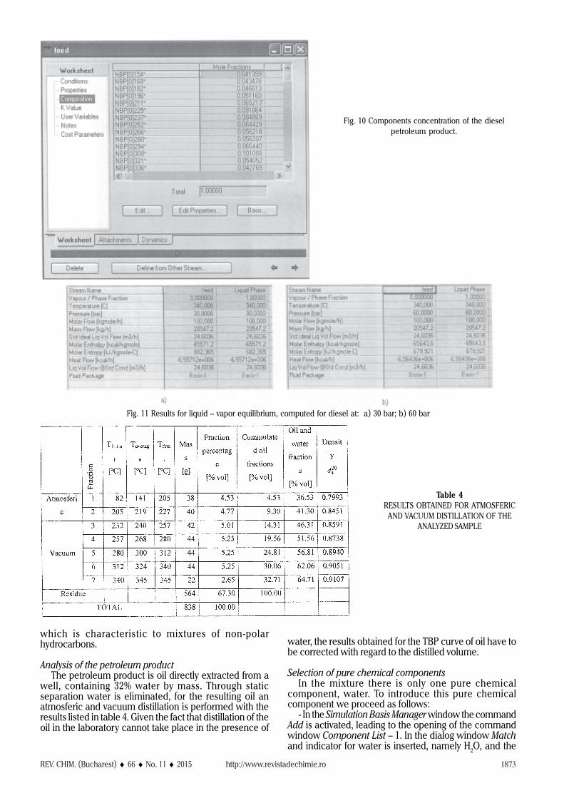
presented before in the case of oil. The concentrations ofthe pseudocomponents in the diesel flux, computed bythe simulator, can be visualized with the help ofComposition command from the Worksheet window (fig.10).

Fig. 8 Physical properties of thepseudocomponents associated to the

petroleum product

Fig. 9 Comparison betweencomputed and experimental ASTM

curve

Simulation of the liquid-vapor equilibrium for dieselThe purpose of the study of liquid – vapor equilibrium for

this petroleum product was that of determining if diesel isin liquid or partially vaporized phase, as well as determiningdiesel properties for the following work conditions:

A.Temperature 340°C and pressure 30 bar ( fig. 11a).B.Temperature 340°C and pressure 60 bar ( fig. 11b).The result shown in figure 11 indicates the fact that the

petroleum product is in liquid phase at the mentionedpressures.

Particularities in defining the component list for oil –water mixture

This case is different when compared to the previousones, requiring a specific approach of the Unisim® simulatorconfiguration. Simulation of the liquid – vapor equilibriumrequires following the stages:

a) selection of the thermodynamic model ;b) analysis of the petroleum product;c) selection of the pure chemical components;d) tnserting in the simulation of laboratory analyses of

the petroleum product;e) computation of the pseudocomponents;f) defining the simulation window;g) simulation of the liquid – vapor equilibrium.

Selection of the thermodynamic modelThe first stage is carried out according to the above-

mentioned mechanism. Because the oil coming from theextraction well contains only hydrocarbons and water, thesame Peng-Robinson thermodynamic model was selected,


Fig. 10 Components concentration of the dieselpetroleum product.

which is characteristic to mixtures of non-polarhydrocarbons.

Analysis of the petroleum productThe petroleum product is oil directly extracted from a

well, containing 32% water by mass. Through staticseparation water is eliminated, for the resulting oil anatmosferic and vacuum distillation is performed with theresults listed in table 4. Given the fact that distillation of theoil in the laboratory cannot take place in the presence of

Fig. 11 Results for liquid – vapor equilibrium, computed for diesel at: a) 30 bar; b) 60 bar

water, the results obtained for the TBP curve of oil have tobe corrected with regard to the distilled volume.

Selection of pure chemical componentsIn the mixture there is only one pure chemical

component, water. To introduce this pure chemicalcomponent we proceed as follows:

- In the Simulation Basis Manager window the commandAdd is activated, leading to the opening of the commandwindow Component List – 1. In the dialog window Matchand indicator for water is inserted, namely H2O, and the

Table 4RESULTS OBTAINED FOR ATMOSFERIC

AND VACUUM DISTILLATION OF THEANALYZED SAMPLE


Add Pure command is activated. The effect of thiscommand is inserting the pure component water in thelist.

Introduction in the simulator of laboratory analyses of thepetroleum product

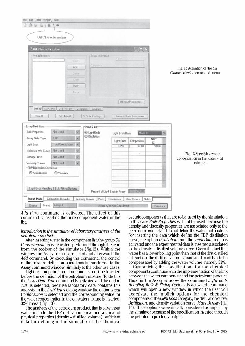
After inserting water in the component list, the group OilCharacterization is activated, performed through the iconfrom the toolbar of the simulator (fig.12). Within thewindow the Assay menu is selected and afterwards theAdd command. By executing this command, the controlof the mixture definition operations is transferred to theAssay command window, similarly to the other use cases.

Light or non-petroleum components must be insertedbefore the definition of the petroleum mixture. To do thisthe Assay Data Type command is activated and the optionTBP is selected, because laboratory data contains thisanalysis. In the Light Ends dialog window the option InputComposition is selected and the corresponding value forthe water concentration in the oil-water mixture is inserted,32% mass ( fig. 13).

The analyses of the petroleum product, that is oil withoutwater, include the TBP distillation curve and a curve ofphysical properties (density – distilled volume), sufficientdata for defining in the simulator of the chemical

Fig. 12 Activation of the OilCharacterization command menu

Fig. 13 Specifying waterconcentration in the water – oil

mixture.

pseudocomponents that are to be used by the simulation.In this case Bulk Properties will not be used because thedensity and viscosity properties are associated only to thepetroleum product and do not define the water – oil mixture.For inserting the data which define the TBP distillationcurve, the option Distillation from the Input Data menu isactivated and the experimental data is inserted associatedto the density – distilled volume curve. Given the fact thatwater has a lower boiling point than that of the first distilledoil fraction, the distilled volume associated to oil has to becompensated by adding the water volume, namely 32%.

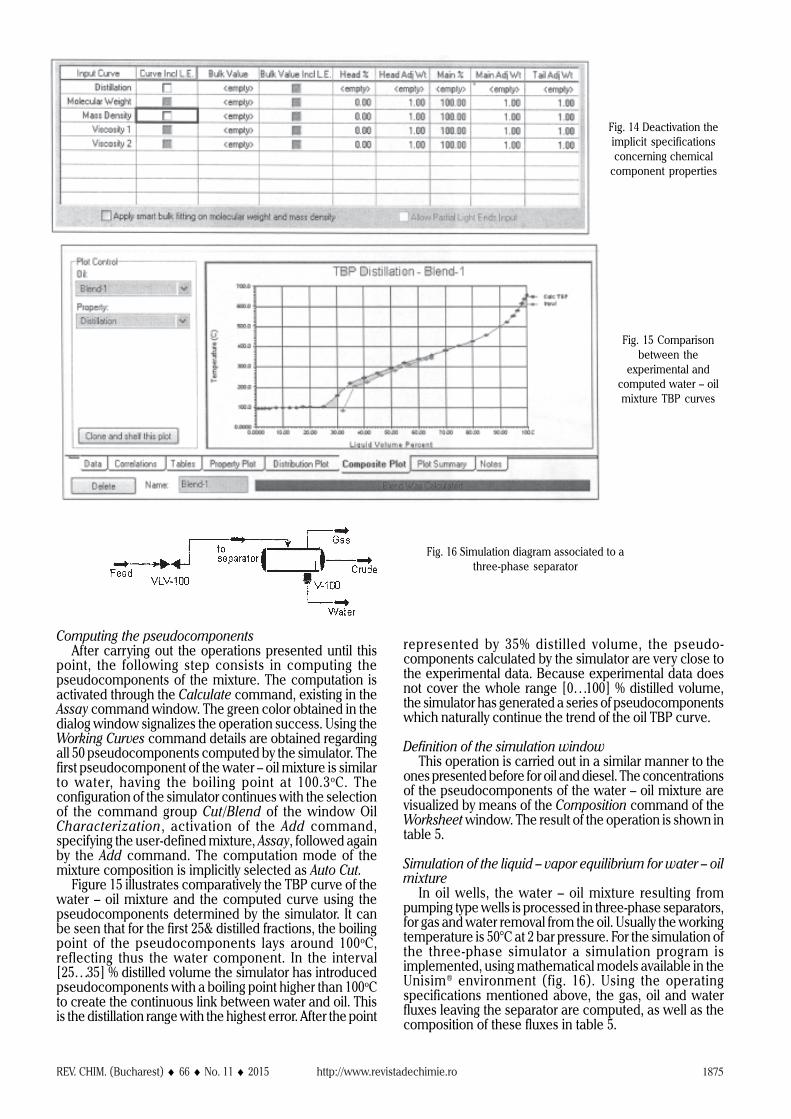
Customizing the specifications for the chemicalcomponents continues with the implementation of the linkbetween the water component and the petroleum product.Thus, in the Assay window the command Light EndsHandling Bulk & Fitting Options is activated, commandwhich will open a new window in which the user willdeactivate the implicit options for the chemicalcomponents of the Light Ends category, the distillation curve,Distillation, and density variation curve, Mass Density (fig.14). These options were initially considered as implicit bythe simulator because of the specification inserted throughthe petroleum product analysis.


Computing the pseudocomponentsAfter carrying out the operations presented until this

point, the following step consists in computing thepseudocomponents of the mixture. The computation isactivated through the Calculate command, existing in theAssay command window. The green color obtained in thedialog window signalizes the operation success. Using theWorking Curves command details are obtained regardingall 50 pseudocomponents computed by the simulator. Thefirst pseudocomponent of the water – oil mixture is similarto water, having the boiling point at 100.3oC. Theconfiguration of the simulator continues with the selectionof the command group Cut/Blend of the window OilCharacterization, activation of the Add command,specifying the user-defined mixture, Assay, followed againby the Add command. The computation mode of themixture composition is implicitly selected as Auto Cut.

Figure 15 illustrates comparatively the TBP curve of thewater – oil mixture and the computed curve using thepseudocomponents determined by the simulator. It canbe seen that for the first 25& distilled fractions, the boilingpoint of the pseudocomponents lays around 100oC,reflecting thus the water component. In the interval[25…35] % distilled volume the simulator has introducedpseudocomponents with a boiling point higher than 100oCto create the continuous link between water and oil. Thisis the distillation range with the highest error. After the point

Fig. 14 Deactivation theimplicit specificationsconcerning chemical

component properties

Fig. 15 Comparisonbetween the

experimental andcomputed water – oilmixture TBP curves

represented by 35% distilled volume, the pseudo-components calculated by the simulator are very close tothe experimental data. Because experimental data doesnot cover the whole range [0…100] % distilled volume,the simulator has generated a series of pseudocomponentswhich naturally continue the trend of the oil TBP curve.

Definition of the simulation windowThis operation is carried out in a similar manner to the

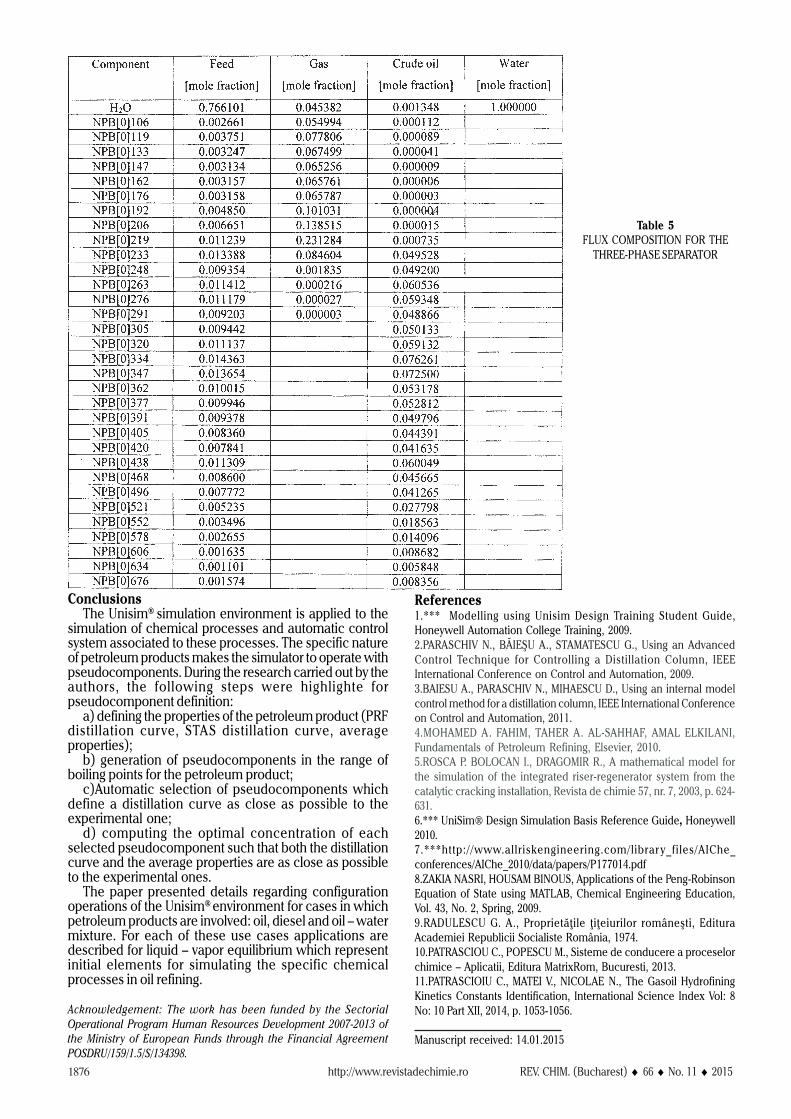
ones presented before for oil and diesel. The concentrationsof the pseudocomponents of the water – oil mixture arevisualized by means of the Composition command of theWorksheet window. The result of the operation is shown intable 5.

Simulation of the liquid – vapor equilibrium for water – oilmixture

In oil wells, the water – oil mixture resulting frompumping type wells is processed in three-phase separators,for gas and water removal from the oil. Usually the workingtemperature is 50°C at 2 bar pressure. For the simulation ofthe three-phase simulator a simulation program isimplemented, using mathematical models available in theUnisim® environment (fig. 16). Using the operatingspecifications mentioned above, the gas, oil and waterfluxes leaving the separator are computed, as well as thecomposition of these fluxes in table 5.

Fig. 16 Simulation diagram associated to athree-phase separator


Table 5FLUX COMPOSITION FOR THE

THREE-PHASE SEPARATOR

ConclusionsThe Unisim® simulation environment is applied to the

simulation of chemical processes and automatic controlsystem associated to these processes. The specific natureof petroleum products makes the simulator to operate withpseudocomponents. During the research carried out by theauthors, the following steps were highlighte forpseudocomponent definition:

a) defining the properties of the petroleum product (PRFdistillation curve, STAS distillation curve, averageproperties);

b) generation of pseudocomponents in the range ofboiling points for the petroleum product;

c)Automatic selection of pseudocomponents whichdefine a distillation curve as close as possible to theexperimental one;

d) computing the optimal concentration of eachselected pseudocomponent such that both the distillationcurve and the average properties are as close as possibleto the experimental ones.

The paper presented details regarding configurationoperations of the Unisim® environment for cases in whichpetroleum products are involved: oil, diesel and oil – watermixture. For each of these use cases applications aredescribed for liquid – vapor equilibrium which representinitial elements for simulating the specific chemicalprocesses in oil refining.

Acknowledgement: The work has been funded by the SectorialOperational Program Human Resources Development 2007-2013 ofthe Ministry of European Funds through the Financial AgreementPOSDRU/159/1.5/S/134398.

References1.*** Modelling using Unisim Design Training Student Guide,Honeywell Automation College Training, 2009.2.PARASCHIV N., BÃIEªU A., STAMATESCU G., Using an AdvancedControl Technique for Controlling a Distillation Column, IEEEInternational Conference on Control and Automation, 2009.3.BAIESU A., PARASCHIV N., MIHAESCU D., Using an internal modelcontrol method for a distillation column, IEEE International Conferenceon Control and Automation, 2011.4.MOHAMED A. FAHIM, TAHER A. AL-SAHHAF, AMAL ELKILANI,Fundamentals of Petroleum Refining, Elsevier, 2010.5.ROSCA P. BOLOCAN I., DRAGOMIR R., A mathematical model forthe simulation of the integrated riser-regenerator system from thecatalytic cracking installation, Revista de chimie 57, nr. 7, 2003, p. 624-631.6.*** UniSim® Design Simulation Basis Reference Guide, Honeywell2010.7.***http://www.allriskengineering.com/librar y_files/AIChe_conferences/AIChe_2010/data/papers/P177014.pdf8.ZAKIA NASRI, HOUSAM BINOUS, Applications of the Peng-RobinsonEquation of State using MATLAB, Chemical Engineering Education,Vol. 43, No. 2, Spring, 2009.9.RADULESCU G. A., Proprietãþile þiþeiurilor româneºti, EdituraAcademiei Republicii Socialiste România, 1974.10.PATRASCIOU C., POPESCU M., Sisteme de conducere a proceselorchimice – Aplicatii, Editura MatrixRom, Bucuresti, 2013.11.PATRASCIOIU C., MATEI V., NICOLAE N., The Gasoil HydrofiningKinetics Constants Identification, International Science Index Vol: 8No: 10 Part XII, 2014, p. 1053-1056.

Manuscript received: 14.01.2015

Documents

Petroleum Fractions Liquid – Vapor Equilibrium Simulation using Unisim Design C.pdf 11 15.pdf · · 2015-11-11Petroleum Fractions Liquid – Vapor Equilibrium Simulation using