Embed Size (px)
Citation preview
1
Pharmaceutical Engineering: Optimization of a Pharmaceutical
Formulation Michelle Bai
Melissa Gordon
Amolika Gupta
Aditya Kommi
Abstract
The effects of magnesium stearate
(MgSt) and shear stress on flow properties
and hydrophobicity are not well known.
Blends with different concentrations of
magnesium stearate and varying amounts
of shear were tested using three different
procedures: the FT4 Rheometer test, a tap
density analyzer, and the Washburn
method, to better understand the relation of
lubricant concentration, amount of shear,
hydrophobicity, and flow properties. The
Freeman Technology FT4 Powder
Rheometer data showed that the blend with
0.00% MgSt concentration had the poorest
flow properties and the 2.00% MgSt blend
had the best flow properties. The tap
density test revealed no correlation
between flow properties and MgSt
concentrations or amount of shear,
however these results may not be accurate
due to limited number of trials. The
Washburn method shows that increasing
the amount shear stress correlates with an
increase in hydrophobicity and vice versa.
Similarly, the Washburn method showed a
clear correlation between the concentration
of MgSt and hydrophobicity.
1. Introduction
The majority of pharmaceutical
products are solid dosage forms, making
the physical and chemical properties of
powders an important focus for the
pharmaceutical industry. The properties
of the multiple powder components that
go into any pharmaceutical formulation
affect both the manufacturing process and
the overall quality of the final product.
These may also affect the drug’s
solubility, the critical quality attribute
that ultimately determines when, where,
and how quickly the drug dissolves in the
body. This changes the bioavailability
and the therapeutic effectiveness of the
drug.
Two specific properties that will be
the focus of this project are the
concentration of the lubricant magnesium
stearate in the blend as well as the shear
applied to the lubricated powder blend;
however, little is known about how these
affect both hydrophobicity and flow
properties, which affect solubility and
processability respectively.
To gain a better understanding of
these relationships, five powder blends,
comprised of varying concentrations of
the lubricant MgSt and the filler lactose,
were sheared to three differing amounts.
By analyzing these properties, a clearer
correlation between the aforementioned
properties, hydrophobicity, and flow
behaviors may be established, thereby
shedding more light on factors that
should be considered in the
manufacturing of tablets.

2
2. Background
Pharmaceutical products are
comprised of two fundamental types of
components: the active pharmaceutical
ingredients (API) and excipients,
typically in the powder form. The API is
the substance that ultimately leads to a
physiological response associated with a
desired therapeutic effect. Additionally,
excipients include a multitude of inert
substances that serve as fillers,
flavorings, binding agents, and
lubricants.
2.1 Materials Utilized
For this particular project, APIs were
excluded from the blends for safety.
Instead, only excipients, specifically
lactose, which serves as a filler, and
magnesium stearate, which serves as a
lubricant were a part of the formulations.
Lactose, a sugar commonly found in
dairy products, gives the tablet most of its
volume. This fact not only eases the
manufacturing process, but it also eases
ingestion1. Lactose is physically a fine,
white powder. Another excipient utilized
in this lab was magnesium stearate, a
lubricant used ensure that tablets are
easily ejected from the machinery.
2.2 Final Product Quality Attributes: Hydrophobicity and Flow Properties
Both hydrophobicity and flow
properties affect the overall quality of the
product. Specifically, hydrophobicity
can affect the release rate of the drug in
the body, determining its effectiveness.
Flow properties are also critical in
optimizing a pharmaceutical formula:
they are how well the powder can move
and are dependent on a multitude of
factors, such as particle size and particle
composition. However, flow properties
are of more importance during the
manufacturing process, as they affect
how the powder progresses throughout
the process. Smaller particles cause the
powder to flow poorly due to more
interactions between them, such as van
der Waals interactions. Ultimately, these
prevent free movement. The opposite is
also true: larger particles cause the
powder to flow in a more fluid-like
manner.
2.3 Shearing
Shearing is the external force acting
on a substance or surface exactly parallel
to the plane in which it lies. Applying
shear force on powders reduces the
particle size so that the powder is finer. In
other words, shearing is used to achieve
de-agglomeration. Typically, shear stress
is applied to the powder with multiple
metal blades in a shear device, and the
powder particles are scraped against each
other. Varying amounts of shear may
change a tablet’s measured
hydrophobicity and flow property values.
Shearing in the laboratory is
representative of the milling process
where mechanical impact may affect
particle size reduction and dissolution
rates of the powders. While shear does
not always have an effect, the use of a
lubricant may affect hydrophobicity, so
adding MgSt to the blend requires
quantification of the amount of shear.
2.4 Using the Carr Index to Compare
Flow Properties
Also known as the compressibility
index, the Carr index is a method used to
determine the flowability of a powder.
The formula includes a ratio of the bulk
density, the density of powder before
compression, to tap density, the density
3
of the powder after compression, to
produce the answer. The equation is as
follows2:
𝐶𝑎𝑟𝑟 𝐼𝑛𝑑𝑒𝑥 = 100(1 −𝐵𝐷
𝑇𝐷)
where BD represents bulk density and
where TD represents tap density.
When the Carr index is lower, the
powder has better flow properties and is
more fluid-like; the opposite is true as
well. The Carr index values are rated on a
scale: values from 5 to 15 indicate
excellent flow properties, 16 to 18
indicate fair flow, and values above 23
indicate poor flow2.
2.5 Using the Washburn Method to
Compare Hydrophobicity
The Washburn method utilizes
capillary action to measure the
hydrophobicity of a powder. When a
powder is hydrophobic, not as much
water enters the column because the
powder and water repel each other. On
the other hand, if a powder is more
hydrophilic more water enters the
column. By comparing the change in
mass of the columns and the speed that
the water enters, the relative
hydrophobicity of a powder can be
determined. The Washburn equation is as
follows3:
where t is time, m is mass, η is the liquid
viscosity, C is a constant so long as the
particle size does not change, ρ is liquid
density, γ is the surface tension of the
liquid, and θ is the angle between the
solid and the liquid. For the purpose of
this project, these constants were
considered collectively, which provided
the slope of the Washburn method curve.
2.6 Using Mohr’s Circle Analysis and
Yield Locus for FT4 Rheometer
Analysis
Mohr’s Circle analysis is a tool that is
used for quantifying powder flow
properties using the unconfined yield
stress (UYS) and the major principle
stress (MPS). The UYS is the shear stress
needed to fracture a consolidated powder
mass to initialize flow. The MPS is the
force used to consolidate the powder
mass. On a graph, the intersection of the
small semicircle, tangent to the best fit
lines, on the x-axis is the value of UYS
and the intersection of the larger circle,
also tangent to the best fit lines, on the x-
axis is the MPS (see figure 29 in
appendix). The ratio of the MPS to UYS
is flow function coefficient (FFC), which
ranks flowability on a scale of 4 to 10,
where 4 is very cohesive and 10 is better
flow6. Generally, the closer the powder’s
flow function is to the x-axis, the more
easily the powder will flow. The UYS
and MPS can also be used to determine
the strength of bridges on hoppers, used
in processing of powders and granules in
the industry. Determining the strength of
bridges may help design hoppers that rid
the blockage of powder flow4.
The yield locus is the amount of
pressure that must be applied before the
powder “yields” or begins to flow. The
data from the shear cell, which shows the
relationship between normal stress and
shear stress, was plotted to define the
yield locus, the slope of the best fit line of
the points plotted. On a scale of 0-10, the
4
higher the yield locus, the more free-
flowing the powder4.
3. Methods/Experimental Design
To measure the hydrophobicity and
flow properties of the powder blends,
three tests were used: the Washburn
method to measure hydrophobicity, tap
density to measure flow properties, and
the Freeman Technology shear cell to
also measure flow properties. Five
blends, each sheared at either 0
revolutions, 160 revolutions, or 640
revolutions, were utilized in these tests.
3.1 Blending the Powders
In order to determine the effect of
different concentrations of MgSt on
hydrophobicity and flow properties, five
blends with concentrations of 2.00%,
1.00%, 0.50%, 0.25%, and 0.00% of
MgSt were made. The 4.5 L - 5.0 L V-
blender was then filled 2/3 of the way with
the 2.00% MgSt blend, determined to be
2 kg upon calculating the blend’s bulk
density. 40g of the blend was MgSt while
the remaining 1960g was lactose.
The blending speed was then set to
the setting of six, or 15.79 RPM, for 20
minutes. This process was repeated for
each of the four other blends.
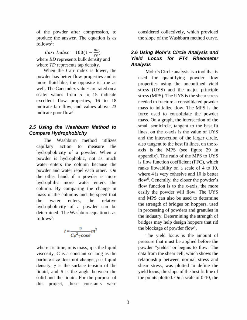
The Patterson Kelley V-Blender
(refer to Figure 1) was used to uniformly
distribute the MgSt in the lactose blend.
3.2 Shearing the Blends
The blends were sheared at varying
amounts: 0 revolutions, 160 revolutions,
or 640 revolutions at 80 RPM.
For each blend, approximately
300.00g was measured and placed into
the Metropolitan Computing Corporation
shear device. Then, the device was either
run for two minutes to achieve 160
revolutions or for eight minutes for 640
revolutions. These sheared samples were
then transferred to their appropriate
Ziploc bags.
Figure 1: Pictured above is the V-blender, used in
the pharmaceutical industry to thoroughly blend
powders.
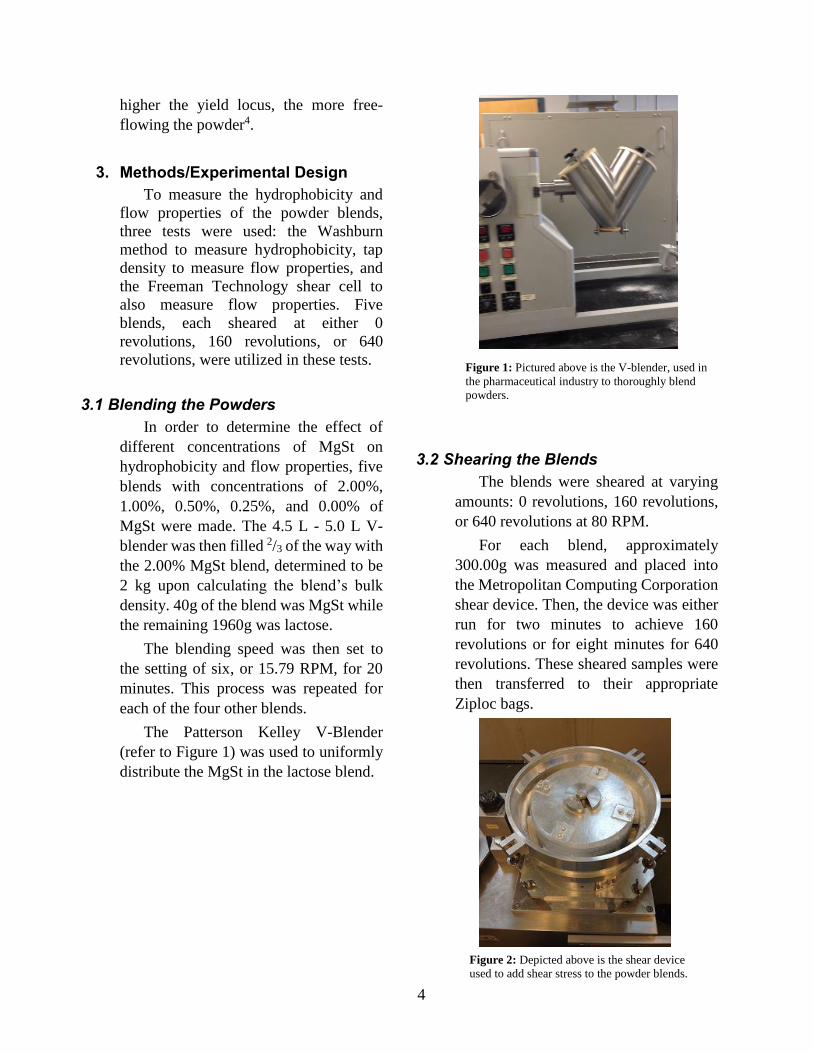
Figure 2: Depicted above is the shear device
used to add shear stress to the powder blends.
5
The custom-made shear device
consists of concentric cylinders with an
annular gap. Both the inner and the outer
cylinder contain symmetric teeth. While
the inner cylinder rotates, the outer wall
is stationary and the rapid spinning of the
teeth and powders against each other
results in shear.
3.3 Measuring Hydrophobicity using the Washburn Method
To create the saturated lactose
solution necessary for the Washburn
method, a solution was created with 350g
lactose in 1400 mL of water at 40°C. In
order to maintain this temperature, the
beaker with the solution was kept
overnight on a hot plate. Additionally, a
magnetic stirring rod was placed in the
solution to ensure thorough mixing,
which allows blend to achieve
equilibrium.
The saturated solution was then
poured through filter paper, which lined a
funnel, into the Erlenmeyer flask. This
was done to remove the undissolved
lactose. A solution was used instead of
water because the super-saturated
solution would prevent any lactose in the
column from dissolving in the solvent
during the tests. The filtered saturated
lactose solution inside the beaker was
then used for measuring hydrophobicity.
The hydrophobicity of the powder
blend was determined by measuring the
rate of the saturated solution moving up a
Washburn column.
The powder blend was initially
tapped 1000 times in the Auto Tap
Density Analyzer machine to compact the
powder tightly in the Washburn column.
The powder blend was then attached to a
ring stand by means of a ring clamp and
lowered into a beaker of the saturated
lactose solution. This entire apparatus
was placed on a balance and connected to
Ohaus Explorer Pro, which measured the
increase in mass. This process was
monitored for 35 minutes and completed
for each of the 15 blends.
3.4 Testing for Tap Density and Bulk
Density
Tap density testing is used for
measuring compaction of different
blends. In order to do this, the initial
volume of a certain powder blend was
measured in a graduated cylinder. Using
the Auto Tap Density Analyzer machine,
the blend was tapped at a constant rate of
260 taps per minute. Changes in volume
were recorded at 20 tap increments for the
first 100 taps, then 50 tap increments for
the second 100 taps, and then at 100 tap
increments for the remaining 800 taps.
All 15 blends went through this process.
3.5 Using the Freeman Technology
Shear Cell to Test Flow Properties
In order to test the resistance of
powder blends to flow movement, the
Freeman Technology 4 (FT4) Rheometer
was utilized to conduct the shear test,
which measured the powder’s behavior
from no-flow to flow state.
The testing required approximately
10 grams of the powder blend, which was
placed in a vessel. This was then placed
in the machine and under a piston. Before
testing can began, the powder
experienced pre-shear conditioning,
achieved by a spinning blade that lowered
into the powder. This created consistency
in shear with each test. Then, the blending

6
blade was switched for the vented piston,
which was used to apply a normal stress
of 3 kPa to the blend. After, the top half
of the vessel was opened so that the
excess powder could be removed to
ensure a consistent and exact volume.
Subsequently, the vented piston was
replaced by the shear cell piston, which
began to move at a low speed. Once it was
lowered into the powder, stress was
slowly applied and increased until the
shear cell was able to move the powder
and caused it to flow.
This test was repeated for 4 samples:
0.00% MgSt, 0.50% MgSt, 1.00% MgSt,
and 2.00% MgSt. All were sheared at 80
RPM for 160 revolutions.
4. Results and Discussion
This experiment aimed to define a
clear relationship between physiological
properties of pharmaceutical tablets, like
MgSt concentration and shear stress, and
final quality attributes of the tablets,
including hydrophobicity and flow
properties.
4.1 FT4 Rheometer Results
The FT4 Rheometer results provided
information on yield locus, flow function
coefficient, cohesion, and Mohr’s Circle
Analysis4.
Based on the results seen in the table
for the FT4 Rheometer (refer to Figure 13
in the Appendix), the powder blend with
0.00% MgSt had the lowest FFC of
3.131. The powder blend with 2.00%
MgSt had the highest FFC of 4.592. In
order from most cohesive blend to most
free flowing, the blends are ranked as
0.00%, 0.50%, 1.00%, and 2.00% MgSt.
4.2 Tap Density Results
Concentration of MgSt Amount of Shear Added
(in revolutions)
Carr Index
0.00% MgSt 0 rev 23.770 – 23.970
160 rev 26.443 – 26.643
640 rev 22.926 – 23.126
0.25% MgSt 0 rev 23.618 – 23.818
160 rev 24.900 – 25.100
640 rev 15.773 – 15.973
0.50% MgSt 0 rev 24.267 – 24.467
160 rev 22.073 – 23.073
640 rev 20.603 – 20.803
1.00% MgSt 0 rev 21.233 – 21.433
160 rev 19.324 – 19.524
640 rev 21.438 – 21.438
2.00% MgSt 0 rev 22.268 – 22.468
160 rev 20.448 – 20.648
640 rev 22.926 – 23.126
The Carr Index values for each blend
were determined using the raw data of the
tap density test, which can be seen in
Figures 6 through 10 in the Appendix. The
0.25% MgSt blend with 640 revolutions
had the lowest Carr Index value of 15.773-
15.973. The only other Carr Index value
under 20.000 was that of 1.00% MgSt with
160 revolutions. On the other hand, all of
the 0.00% MgSt samples, the 0.25% MgSt
blend with 0 revolutions, the 0.25% MgSt
blend with 160 revolutions, the 0.50%
MgSt sample with 0 revolutions, and the
2.00% MgSt sample with 640 revolutions
have Carr Index values that exceed 23.000,
the minimum value needed for a powder to
be considered poor-flowing.
4.3 Washburn Method Results
The slopes from each of the
Washburn graphs (refer to Figures 11
through 28 in the Appendix) provide the
relationship regarding the hydrophobicity
of the powder formulation that was tested.
Figure 3: The above table displays the Carr Index values
for all 15 samples. There is a 0.2 mL range for each value
to account for the uncertainty in the tap density volume
measurements.

7
The blend with the highest slope is the
0.50% MgSt at 640 revolutions, which has
an R2 value of 0.8554. Conversely, the
powder with the lowest slope is the 2.00%
MgSt at 640 revolutions, and its R2 value is
0.9997.
Of all of the graphs, ten blends had
low slopes that were less than one. This
includes all five blends without shear
stress. Similarly, three blends at 160
revolutions had these smaller slopes: 0.00%
MgSt, 0.25% MgSt, and 2.00% MgSt. Two
blends at 640 revolutions experienced this
as well.
4.4 Comparison of MgSt Concentration, Shear Stress, Hydrophobicity, and Flow Properties
The blends can be ranked, in order
from least to most free-flowing, as
0.00%, 0.50%, 1.00%, and 2.00% MgSt.
It can therefore be deduced that the
presence of MgSt improves a powder’s
flow properties. The powder blend with
no MgSt does not contain any lubricant
and is hence much more cohesive. The
FFC correlates with cohesion, measured
in kPa: the lower the FFC value, the
higher the cohesion.
The results from the tap density test
show no correlation for flow properties
and magnesium stearate concentration.
This differs from other studies by Pingali,
Podczeck, and Velasco. These authors
agreed that changing the concentration of
lubricant changes flowability4.
There also appears to be no well-
defined correlation between the amount
of shear stress applied to the blends and
flow properties. Other studies by
Pingali have shown that flow properties
decrease as amount of shear increases4.
This can be explained by the fact that
shearing makes the particles in the
powder smaller, which makes it harder
for the powders to flow.
This lack of a correlation was
determined using ANOVA tests—one for
shear stress and one for concentration of
MgSt. It was determined that there were
no significant statistical differences in
Carr Index values in either case.
Therefore, there is no distinct correlation
between varying concentrations of MgSt
and flow properties or between varying
amounts of shear stress and flow
properties that can be seen from this test.
The data collected from the
Washburn Method shows there is a direct
correlation between hydrophobicity and
the amount of shear stress applied to the
blends (refer to Figures 6 through 10). As
the amount of shear stress increased, the
hydrophobicity also increased. In the
0.50% MgSt blend sample with no shear
stress, the slope was 0.9606, while the
slope of the sample sheared for 640
revolutions had a slope of 3.5504. The
increase in slope directly correlates with
hydrophobicity. This relationship was
predicted as shearing results in smaller
particles, resulting in more interactive
forces between the particles. This
increase in hydrophobicity is consistent
with other studies4.
The Washburn Method also showed a
direct correlation between the amount of
Figure 5: This table contains ANOVA values, used
to explain the lack of a correlation between amount
of shear stress and flow properties.
Figure 4: This table contains ANOVA values,
used to explain the lack of a correlation
between the concentration of MgSt and flow
properties.
8
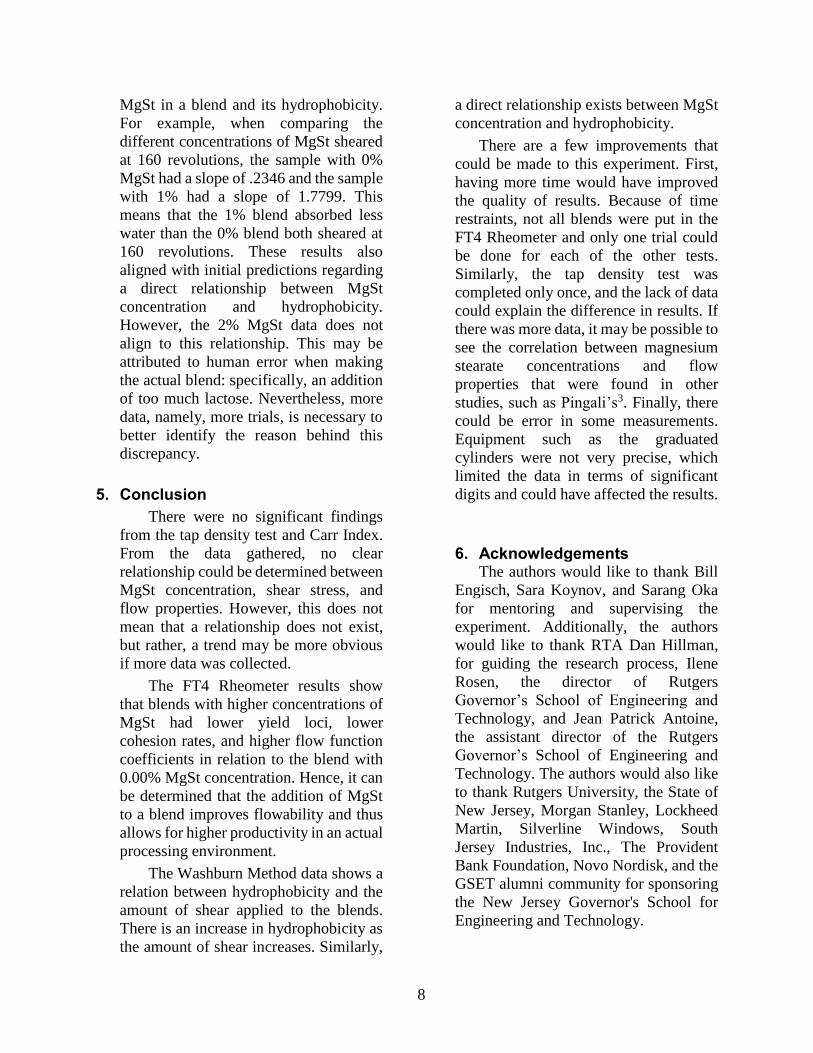
MgSt in a blend and its hydrophobicity.
For example, when comparing the
different concentrations of MgSt sheared
at 160 revolutions, the sample with 0%
MgSt had a slope of .2346 and the sample
with 1% had a slope of 1.7799. This
means that the 1% blend absorbed less
water than the 0% blend both sheared at
160 revolutions. These results also
aligned with initial predictions regarding
a direct relationship between MgSt
concentration and hydrophobicity.
However, the 2% MgSt data does not
align to this relationship. This may be
attributed to human error when making
the actual blend: specifically, an addition
of too much lactose. Nevertheless, more
data, namely, more trials, is necessary to
better identify the reason behind this
discrepancy.
5. Conclusion
There were no significant findings
from the tap density test and Carr Index.
From the data gathered, no clear
relationship could be determined between
MgSt concentration, shear stress, and
flow properties. However, this does not
mean that a relationship does not exist,
but rather, a trend may be more obvious
if more data was collected.
The FT4 Rheometer results show
that blends with higher concentrations of
MgSt had lower yield loci, lower
cohesion rates, and higher flow function
coefficients in relation to the blend with
0.00% MgSt concentration. Hence, it can
be determined that the addition of MgSt
to a blend improves flowability and thus
allows for higher productivity in an actual
processing environment.
The Washburn Method data shows a
relation between hydrophobicity and the
amount of shear applied to the blends.
There is an increase in hydrophobicity as
the amount of shear increases. Similarly,
a direct relationship exists between MgSt
concentration and hydrophobicity.
There are a few improvements that
could be made to this experiment. First,
having more time would have improved
the quality of results. Because of time
restraints, not all blends were put in the
FT4 Rheometer and only one trial could
be done for each of the other tests.
Similarly, the tap density test was
completed only once, and the lack of data
could explain the difference in results. If
there was more data, it may be possible to
see the correlation between magnesium
stearate concentrations and flow
properties that were found in other
studies, such as Pingali’s3. Finally, there
could be error in some measurements.
Equipment such as the graduated
cylinders were not very precise, which
limited the data in terms of significant
digits and could have affected the results.
6. Acknowledgements
The authors would like to thank Bill
Engisch, Sara Koynov, and Sarang Oka
for mentoring and supervising the
experiment. Additionally, the authors
would like to thank RTA Dan Hillman,
for guiding the research process, Ilene
Rosen, the director of Rutgers
Governor’s School of Engineering and
Technology, and Jean Patrick Antoine,
the assistant director of the Rutgers
Governor’s School of Engineering and
Technology. The authors would also like
to thank Rutgers University, the State of
New Jersey, Morgan Stanley, Lockheed
Martin, Silverline Windows, South
Jersey Industries, Inc., The Provident
Bank Foundation, Novo Nordisk, and the
GSET alumni community for sponsoring
the New Jersey Governor's School for
Engineering and Technology.

9
References 1S. Oka, “Intro to Dosage Forms and
Excipients” Lecture Notes, Rutgers,
Summer 2014 (unpublished) 2“Particle & Powder Density, Index
and Carr Ratio,” Escubed Limited,
<http://www.escubed.co.uk/sites/default/file
s/density_measurement_(an006)_carrs_inde
x_and_hausner_ratio.pdf> (9 July 2014). 3 K. Pingali et al., “Evaluation of
Strain-Induced Hydrophobicity of
Pharmaceutical Blends and Its Effect on
Drug Release Rate under Multiple
Compression Conditions,” Drug
Development and Industrial Pharmacy 37,
428-435 (2011).
4 "Volution Flow Therapy," Mercury
Scientific Incorporated, 2012,
<http://www.mercuryscientific.com/instrum
ents/volution-flow-theory> (24 July 2014).
5 K. Pingali et al., “Evaluation of
Strain-Induced Hydrophobicity of
Pharmaceutical Blends and Its Effect on
Drug Release Rate under Multiple
Compression Conditions,” Drug
Development and Industrial Pharmacy 37,
428-435 (2011).
6 R. Freeman, “Measuring the Flow
of Properties of Consolidated, Conditioned,
and Aerated
Powders — A Comparative Study Using a
Powder Rheometer and a Rotational Shear
Cell,” Physics International 174, 25–33
(2007).
10
Appendix
Taps Volume (mL); ± 0.1 mL
0 rev 160 rev 640 rev
0 81.0 mL 77.5 mL 76.0 mL
20 74.0 mL 72.5 mL 71.0 mL
40 69.5 mL 69.0 mL 67.3 mL
60 66.8 mL 66.0 mL 65.0 mL
80 64.5 mL 64.0 mL 63.0 mL
100 64.0 mL 63.5 mL 62.0 mL
150 62.0 mL 61.5 mL 61.0 mL
200 62.0 mL 61.0 mL 60.5 mL
300 61.0 mL 60.5 mL 60.0 mL
400 61.0 mL 60.0 mL 59.8 mL
500 60.5 mL 59.8 mL 59.5 mL
600 60.0 mL 59.8 mL 59.0 mL
700 60.0 mL 59.5 mL 59.0 mL
800 60.0 mL 59.5 mL 59.0 mL
900 60.0 mL 59.0 mL 58.5 mL
1000 59.5 mL 59.0 mL 58.5 mL
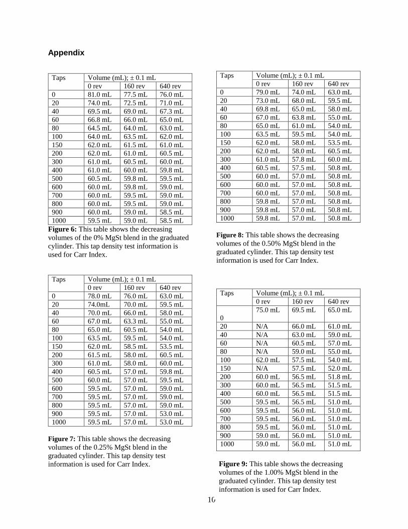
Figure 6: This table shows the decreasing
volumes of the 0% MgSt blend in the graduated
cylinder. This tap density test information is
used for Carr Index.
Taps Volume (mL); ± 0.1 mL
0 rev 160 rev 640 rev
0 78.0 mL 76.0 mL 63.0 mL
20 74.0mL 70.0 mL 59.5 mL
40 70.0 mL 66.0 mL 58.0 mL
60 67.0 mL 63.3 mL 55.0 mL
80 65.0 mL 60.5 mL 54.0 mL
100 63.5 mL 59.5 mL 54.0 mL
150 62.0 mL 58.5 mL 53.5 mL
200 61.5 mL 58.0 mL 60.5 mL
300 61.0 mL 58.0 mL 60.0 mL
400 60.5 mL 57.0 mL 59.8 mL
500 60.0 mL 57.0 mL 59.5 mL
600 59.5 mL 57.0 mL 59.0 mL
700 59.5 mL 57.0 mL 59.0 mL
800 59.5 mL 57.0 mL 59.0 mL
900 59.5 mL 57.0 mL 53.0 mL
1000 59.5 mL 57.0 mL 53.0 mL
Figure 7: This table shows the decreasing
volumes of the 0.25% MgSt blend in the
graduated cylinder. This tap density test
information is used for Carr Index.
Figure 8: This table shows the decreasing
volumes of the 0.50% MgSt blend in the
graduated cylinder. This tap density test
information is used for Carr Index.
Taps Volume (mL); ± 0.1 mL
0 rev 160 rev 640 rev
0
75.0 mL 69.5 mL 65.0 mL
20 N/A 66.0 mL 61.0 mL
40 N/A 63.0 mL 59.0 mL
60 N/A 60.5 mL 57.0 mL
80 N/A 59.0 mL 55.0 mL
100 62.0 mL 57.5 mL 54.0 mL
150 N/A 57.5 mL 52.0 mL
200 60.0 mL 56.5 mL 51.8 mL
300 60.0 mL 56.5 mL 51.5 mL
400 60.0 mL 56.5 mL 51.5 mL
500 59.5 mL 56.5 mL 51.0 mL
600 59.5 mL 56.0 mL 51.0 mL
700 59.5 mL 56.0 mL 51.0 mL
800 59.5 mL 56.0 mL 51.0 mL
900 59.0 mL 56.0 mL 51.0 mL
1000 59.0 mL 56.0 mL 51.0 mL
Taps Volume (mL); ± 0.1 mL
0 rev 160 rev 640 rev
0 79.0 mL 74.0 mL 63.0 mL
20 73.0 mL 68.0 mL 59.5 mL
40 69.8 mL 65.0 mL 58.0 mL
60 67.0 mL 63.8 mL 55.0 mL
80 65.0 mL 61.0 mL 54.0 mL
100 63.5 mL 59.5 mL 54.0 mL
150 62.0 mL 58.0 mL 53.5 mL
200 62.0 mL 58.0 mL 60.5 mL
300 61.0 mL 57.8 mL 60.0 mL
400 60.5 mL 57.5 mL 50.8 mL
500 60.0 mL 57.0 mL 50.8 mL
600 60.0 mL 57.0 mL 50.8 mL
700 60.0 mL 57.0 mL 50.8 mL
800 59.8 mL 57.0 mL 50.8 mL
900 59.8 mL 57.0 mL 50.8 mL
1000 59.8 mL 57.0 mL 50.8 mL
Figure 9: This table shows the decreasing
volumes of the 1.00% MgSt blend in the
graduated cylinder. This tap density test
information is used for Carr Index.

11
Taps Volume (mL); ± 0.1 mL
0 rev 160 rev 640 rev
0 76.0 mL 73.0 mL 76.0 mL
20 71.0mL 69.0 mL 71.0 mL
40 68.0 mL 66.0 mL 68.0 mL
60 64.5 mL 63.0 mL 65.0 mL
80 63.0 mL 61.5 mL 63.3 mL
100 62.0 mL 60.5 mL 62.0 mL
150 61.0 mL 60.0 mL 62.0 mL
200 60.5 mL 59.8 mL 61.0 mL
300 60.0 mL 59.0 mL 60.0 mL
400 59.5 mL 59.0 mL 59.8 mL
500 59.5 mL 58.8 mL 59.5 mL
600 59.5 mL 58.0 mL 59.0 mL
700 59.0 mL 58.0 mL 59.0 mL
800 59.0 mL 58.0 mL 59.0 mL
900 59.0 mL 58.0 mL 59.0 mL
1000 59.0 mL 58.0 mL 58.5 mL
Figure 10: This table shows the decreasing volumes
of the 2.00% MgSt blend in the graduated cylinder.
This tap density test information is used for Carr Index.
Concentration of
MgSt
(%)
Revolutions Variance of
mean
Mean of
Variance
0 160 640
0% 26.543 23.871 23.026
0.25% 23.718 25 15.873
0.5% 24.304 22.973 19.365
1% 21.333 19.424 21.538
2 22.368 20.548 23.026
Mean 23.65 22.36 20.57 2.40479
st dev 1.99 2.32 3.02
variance 3.95 5.38 9.13 6.16
Figure 11: This table describes the calculations needed to determine the F value of the ANOVA
test.

12
Figure 12: This table describes the calculations needed to determine the F value of the ANOVA
test.
Shear Blends
Material
and Batch
Cohesion
(kPa)
UYS
(kPa)
MPS
(kPa) FFC
2% MgSt 160
Rev_25mm_Shear_3kPa
2% MgSt
160 Rev 0.32 kPa 1.19 kPa 5.47 kPa 4.59
1% MgSt 160 Rev
3_25mm_Shear_3kPa
1% MgSt
160 Rev 0.38 kPa 1.29 kPa 5.37 kPa 4.15
0.5% MgSt 160
Rev_25mm_Shear_3kPa
0.5% MgSt
160 Rev 0.39 kPa 1.37 kPa 5.48 kPa 4.00
0% MgSt 160
Rev_25mm_Shear_3kPa
0% MgSt
160 Rev 0.51 kPa 1.81 kPa 5.66 kPa 3.13
Figure 13: This table displays the different values for determining flow properties of the different
samples of blends tested in the FT4 Rheometer.
Shear
(Revolutions)
Concentration of MgSt (%) Mean St Dev Variance
0% 0.25% 0.50% 1.00% 2.00%
0 26.54 23.72 24.30 21.33 22.37 23.65 1.99 3.95
160 23.87 25.00 22.97 19.42 20.55 22.36 2.32 3.95
640 23.03 15.87 19.37 21.54 23.03 20.57 3.02 5.38
Variance of
Mean
2.40
Mean of
Variance
6.16
13
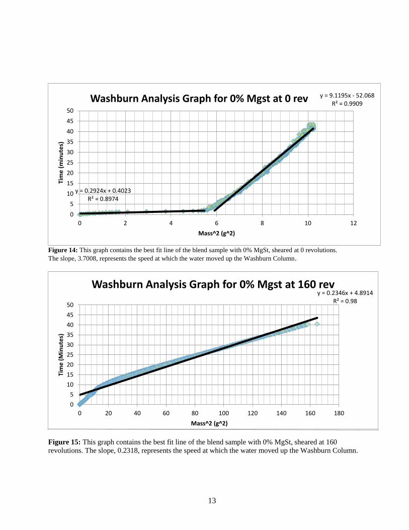
Figure 14: This graph contains the best fit line of the blend sample with 0% MgSt, sheared at 0 revolutions.
The slope, 3.7008, represents the speed at which the water moved up the Washburn Column.
Figure 15: This graph contains the best fit line of the blend sample with 0% MgSt, sheared at 160
revolutions. The slope, 0.2318, represents the speed at which the water moved up the Washburn Column.
y = 0.2924x + 0.4023R² = 0.8974
y = 9.1195x - 52.068R² = 0.9909
0
5
10
15
20
25
30
35
40
45
50
0 2 4 6 8 10 12
Tim
e (
min
ute
s)
Mass^2 (g^2)
Washburn Analysis Graph for 0% Mgst at 0 rev
y = 0.2346x + 4.8914R² = 0.98
0
5
10
15
20
25
30
35
40
45
50
0 20 40 60 80 100 120 140 160 180
Tim
e (
Min
ute
s)
Mass^2 (g^2)
Washburn Analysis Graph for 0% Mgst at 160 rev

14
Figure 16: This graph contains the best fit line of the blend sample with 0% MgSt, sheared at 640
revolutions. The slope, 4.9486, represents the speed at which the water moved up the Washburn Column.
Figure 17: This graph contains the best fit line of the blend sample with 0.25% MgSt, sheared at 0
revolutions. The slope, 0.5538, represents the speed at which the water moved up the Washburn Column.
y = 0.919x - 0.2664R² = 0.9926
-10
0
10
20
30
40
50
60
70
0 1 2 3 4 5 6 7
Tim
e (
Min
ute
s)
Mass^2 (g^2)
Washburn Analysis Graph for 0% Mgst at 640 rev
y = 0.5538x + 0.2341R² = 0.9991
0
5
10
15
20
25
30
35
40
0 10 20 30 40 50 60 70
Tim
e (
Min
ute
s)
Mass2 (g2)
Washburn Method Graph for 0.25% Mgst at 0 rev

15
Figure 18: This graph contains the best fit line of the blend sample with 0.25% MgSt, sheared at 160
revolutions. The slope, 0.5538, represents the speed at which the water moved up the Washburn
Column.
Figure 19: This graph contains the best fit line of the blend sample with 0.25% MgSt, sheared at 640
revolutions. The slope, 3.6894, represents the speed at which the water moved up the Washburn
Column.

16
Figure 20: This graph contains the best fit line of the blend sample with 0.5% MgSt, sheared at 0
revolutions. The slope, 0.8957, represents the speed at which the water moved up the Washburn Column.
Figure 21: This graph contains the best fit line of the blend sample with 0.5% MgSt, sheared at
160 revolutions. The slope, 2.0065, represents the speed at which the water moved up the
Washburn Column.
y = 0.8957x - 1.541R² = 0.9857
-5
0
5
10
15
20
25
30
35
40
45
0 10 20 30 40 50
Min
ute
s
Mass2 (g2)
Washburn Method Graph for 0.5% Mgst at 0 rev
y = 2.0065x - 3.4234R² = 0.9926
-10
0
10
20
30
40
50
0 5 10 15 20 25
Tim
e (
Min
ute
s)
Mass2 (g2)
Washburn Method Graph for 0.5% Mgst at 160 rev
17
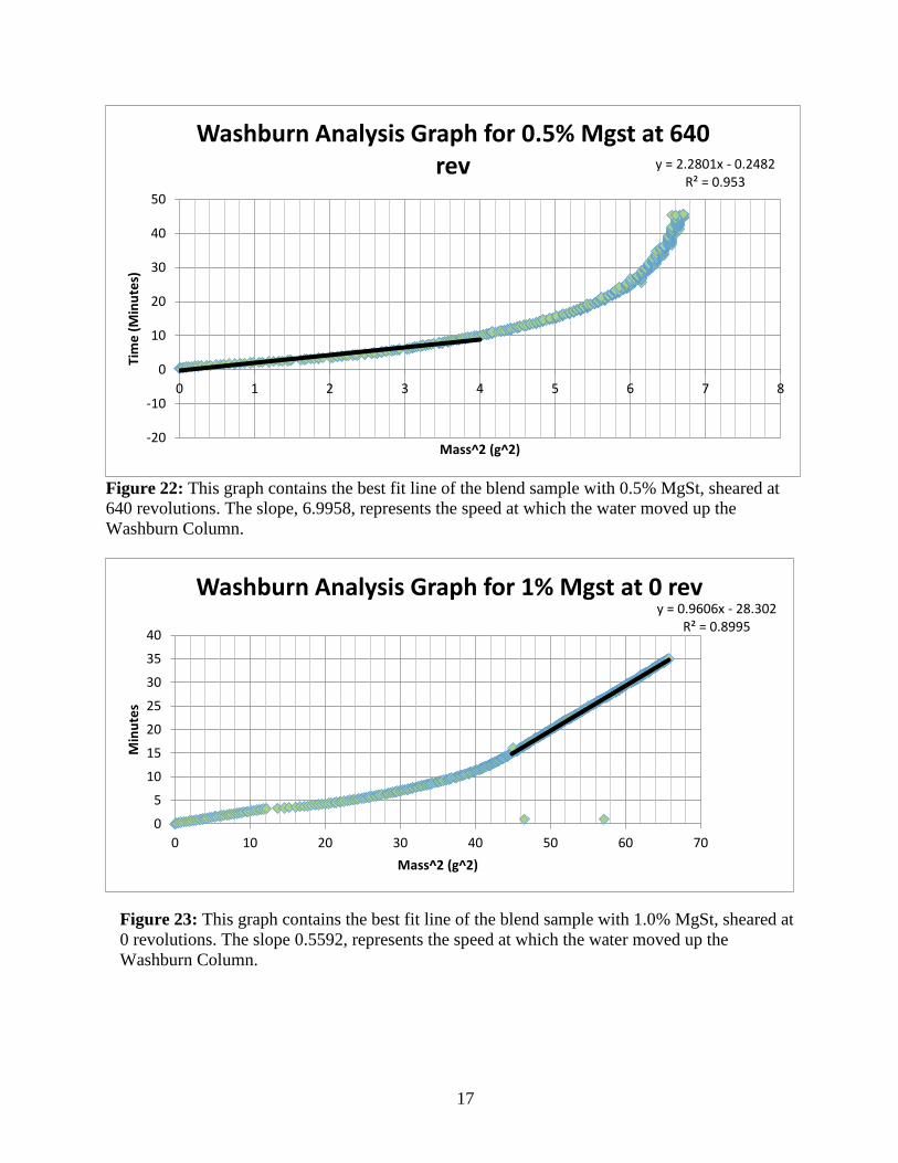
Figure 22: This graph contains the best fit line of the blend sample with 0.5% MgSt, sheared at
640 revolutions. The slope, 6.9958, represents the speed at which the water moved up the
Washburn Column.
y = 2.2801x - 0.2482R² = 0.953
-20
-10
0
10
20
30
40
50
0 1 2 3 4 5 6 7 8
Tim
e (
Min
ute
s)
Mass^2 (g^2)
Washburn Analysis Graph for 0.5% Mgst at 640 rev
y = 0.9606x - 28.302R² = 0.8995
0
5
10
15
20
25
30
35
40
0 10 20 30 40 50 60 70
Min
ute
s
Mass^2 (g^2)
Washburn Analysis Graph for 1% Mgst at 0 rev
Figure 23: This graph contains the best fit line of the blend sample with 1.0% MgSt, sheared at
0 revolutions. The slope 0.5592, represents the speed at which the water moved up the
Washburn Column.

18
Figure 24: This graph contains the best fit line of the blend sample with 1.0% MgSt, sheared at 160
revolutions. The slope, 1.6346, represents the speed at which the water moved up the Washburn Column.
Figure 25: This graph contains the best fit line of the blend sample with 1.0% MgSt, sheared at 640
revolutions. The slope, 3.5281, represents the speed at which the water moved up the Washburn Column.
y = 1.6346x - 5.2957R² = 0.98
-10
-5
0
5
10
15
20
25
30
35
40
0 5 10 15 20 25 30
Tim
e (
Min
ute
s)
Mass2 (g2)
Graph 1.10: Washburn Method Analysis for 1% Mgst at 160 rev
y = 3.5504x - 13.949R² = 0.9988
0
5
10
15
20
25
30
35
40
45
0 2 4 6 8 10 12 14 16 18
Min
ute
s
Mass^2 (g^2)
Washburn Analysis Graph for 1% Mgst at 640 rev
19
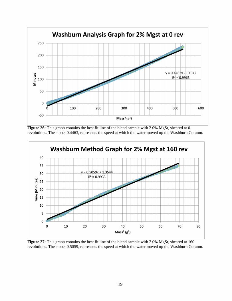
Figure 26: This graph contains the best fit line of the blend sample with 2.0% MgSt, sheared at 0
revolutions. The slope, 0.4463, represents the speed at which the water moved up the Washburn Column.
Figure 27: This graph contains the best fit line of the blend sample with 2.0% MgSt, sheared at 160
revolutions. The slope, 0.5059, represents the speed at which the water moved up the Washburn Column.
y = 0.4463x - 10.942R² = 0.9963
-50
0
50
100
150
200
250
0 100 200 300 400 500 600
Min
ute
s
Mass2 (g2)
Washburn Analysis Graph for 2% Mgst at 0 rev
y = 0.5059x + 1.3544R² = 0.9933
0
5
10
15
20
25
30
35
40
0 10 20 30 40 50 60 70 80
Tim
e (
Min
ute
s)
Mass2 (g2)
Washburn Method Graph for 2% Mgst at 160 rev
20
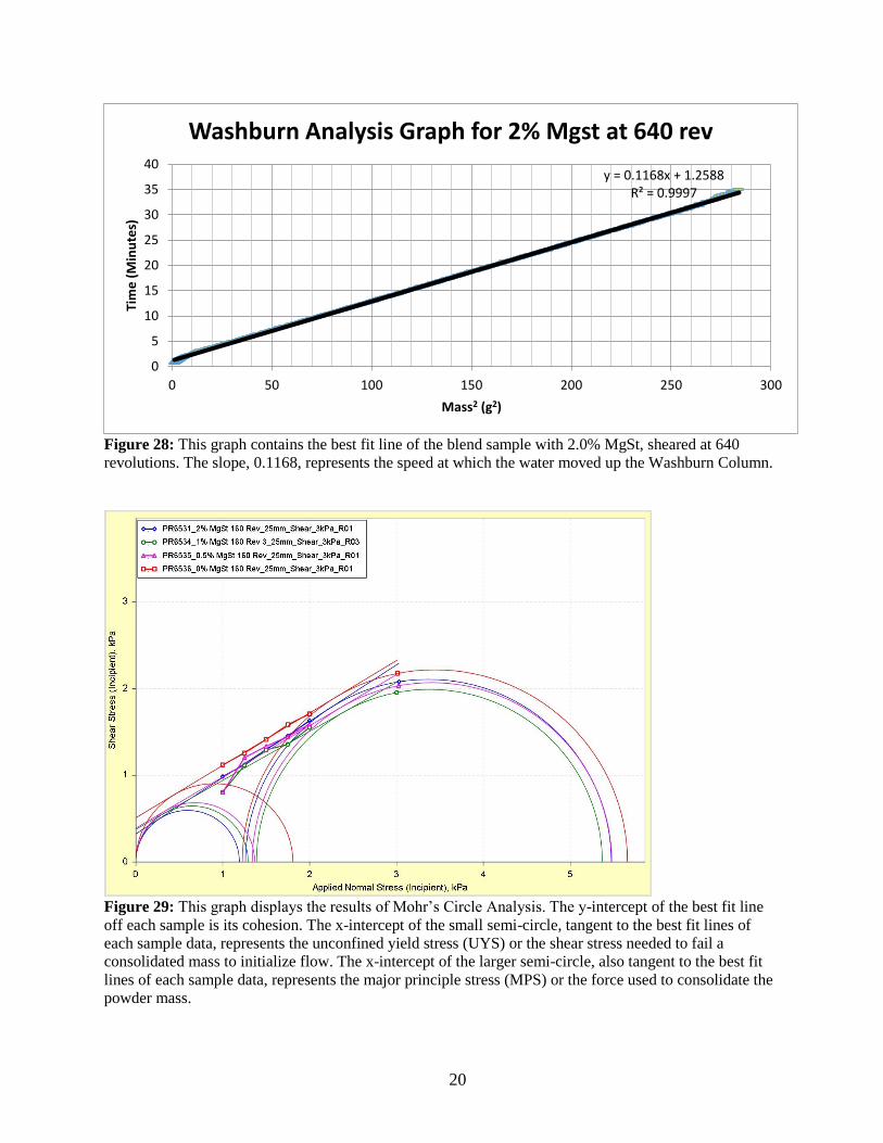
Figure 28: This graph contains the best fit line of the blend sample with 2.0% MgSt, sheared at 640
revolutions. The slope, 0.1168, represents the speed at which the water moved up the Washburn Column.
Figure 29: This graph displays the results of Mohr’s Circle Analysis. The y-intercept of the best fit line
off each sample is its cohesion. The x-intercept of the small semi-circle, tangent to the best fit lines of
each sample data, represents the unconfined yield stress (UYS) or the shear stress needed to fail a
consolidated mass to initialize flow. The x-intercept of the larger semi-circle, also tangent to the best fit
lines of each sample data, represents the major principle stress (MPS) or the force used to consolidate the
powder mass.
y = 0.1168x + 1.2588R² = 0.9997
0
5
10
15
20
25
30
35
40
0 50 100 150 200 250 300
Tim
e (
Min
ute
s)
Mass2 (g2)
Washburn Analysis Graph for 2% Mgst at 640 rev


![Formulation Design, Optimization and Pharmacodynamic ... · July - August 2014 Indian Journal of Pharmaceutical Sciences 355 pharmacodynamic potential[12]. Optimization of pharmaceutical](https://img.pdfslide.net/doc/110x75/5e0eee7778f0721e6f5387a9/formulation-design-optimization-and-pharmacodynamic-july-august-2014-indian.jpg)


![[Power Point] Mixing - Pharmaceutical Engineering](https://img.pdfslide.net/doc/110x75/58f2181a1a28ab637a8b45a5/power-point-mixing-pharmaceutical-engineering.jpg)
![[Paperwork] Mixing - Pharmaceutical Engineering](https://img.pdfslide.net/doc/110x75/58f217e81a28abe2718b45b1/paperwork-mixing-pharmaceutical-engineering.jpg)