Embed Size (px)
Citation preview
Phase 3 MnDOT Slope Vulnerability AssessmentsJen Holmstadt, Principal InvestigatorWSB & Associates, Inc.
July 2020
Research ProjectFinal Report 2020-21
Office of Research & Innovation • mndot.gov/research

To request this document in an alternative format, such as braille or large print, call 651-366-4718 or 1-800-657-3774 (Greater Minnesota) or email your request to [email protected]. Pleaserequest at least one week in advance.

Technical Report Documentation Page 1. Report No.
MN 2020-21 2. 3. Recipients Accession No.
4. Title and Subtitle
Phase 3 MnDOT Slope Vulnerability Assessments 5. Report Date
July 2020 6.
7. Author(s)
Jen Holmstadt, Nick Bradley, Nick Rodgers 8. Performing Organization Report No.
9. Performing Organization Name and Address
WSB & Associates, Inc. 701 Xenia Ave South, Suite 300 Golden Valley, MN 55416
10. Project/Task/Work Unit No.
11. Contract (C) or Grant (G)
(C) 1035395
No.
12. Sponsoring Organization Name and Address
Minnesota Department of Transportation Office of Research & Innovation 395 John Ireland Boulevard, MS 330 St. Paul, Minnesota 55155-1899
13. Type of Report and
Final Report Period Covered
14. Sponsoring Agency Code
15. Supplementary Notes
http://mndot.gov/research/reports/2020/202021.pdf 16. Abstract (Limit: 250 words)
Phase 3 Slope Vulnerability Assessments is a continuation of Phases 1 and 2 previously conducted by WSB and MnDOT to determine the risk of slope failure along state highways. This phase includes 27 counties located in MnDOT districts 1, 2, 3, and 4. The three main components of the model are 1) identify past slope failures, 2) model the causative factors of past slope failures and how they vary locally, and 3) model the risk of new slope failures. Vulnerability factors, failure types, and model results reflect the geomorphology of this region. Vulnerability factors for the new study area include slope angle, terrain curvature, and water table depth. Field verification validates the model’s capability of identifying risk in regions with different geology, geomorphology, and hydrology including deep-seated slides. Model results were ranked into four proposed risk management categories: action recommended, further evaluation, monitoring, and no action recommended. The risk estimation process for this phase is considered preliminary; further consideration of risk tolerance and consequence definitions should be conducted. Preliminary risk results indicate that 370 management areas, and 3% of the total area falls into the action recommended category under the proposed risk matrix. The results of this study are intended to be the first step of actions required in minimizing the effects of slope failure including expensive mitigation and maintenance repairs and threats to public safety.
17. Document Analysis/Descriptors
Slopes, Risk assessments, landslides, erosion, geotechnical engineering, geomorphology, geographic information systems, mathematical models
18. Availability Statement
No restrictions. Document available from: National Technical Information Services, Alexandria, Virginia 22312
19. Security Class
Unclassified (this report) 20. Security Class
Unclassified (this page) 21. No. of Pages
36 22. Price
PHASE 3 MNDOT SLOPE VULNERABILITY ASSESSMENTS
FINAL REPORT
Prepared by:
Jen Holmstadt
Nick Bradley
Nick Rodgers
WSB & Associates, Inc.
JULY 2020
Published by:
Minnesota Department of Transportation
Office of Research & Innovation395 John Ireland Boulevard, MS 330
St. Paul, Minnesota 55155-1899
This report represents the results of research conducted by the authors and does not necessarily represent the views or policies
of the Minnesota Department of Transportation or WSB & Associates, Inc. This report does not contain a standard or specified
technique.
The authors, the Minnesota Department of Transportation, and WSB & Associates, Inc. do not endorse products or
manufacturers. Trade or manufacturers’ names appear herein solely because they are considered essential to this report.

ACKNOWLEDGMENTS
WSB would like to acknowledge Raul Velasquez and Katie Fleming. Their contributions and guidance
were invaluable. WSB would also like to acknowledge members of the Technical Advisory Panel for their
time, ideas, and positive contributions to the final project: Nathan Bausman, James Bittmann, Chris
Dulian, Shannon Foss, Bernard Izevbekhai, Sara Johnson, Blake Nelson, Tony Runkel, Andrew
Shinnefield, Amy Thorson, and Jennifer Wiltgen.
TABLE OF CONTENTS
CHAPTER 1: Introduction ...................................................................................................................... 1
1.1 Phases 1 and 2 Summary .................................................................................................................... 1
CHAPTER 2: Task 2 Literature Review ................................................................................................... 2
2.1 Geomorphology .................................................................................................................................. 2
2.1.1 Geomorphic History of Low Relief Glacial Lake Agassiz in Northwest Minnesota...................... 2
2.1.2 Geomorphic History of Hummocky Terrain in Northcentral Minnesota .................................... 3
CHAPTER 3: Task 3 Model Design ......................................................................................................... 4
3.1 Historical Slope Failures Model .......................................................................................................... 4
3.1.1 Deep-Seated Slides in Lake Agassiz Clay ..................................................................................... 4
3.2 Causative Factors ................................................................................................................................ 5
3.2.1 Water Table Depth ...................................................................................................................... 6
3.2.2 Distance to Lakes ......................................................................................................................... 6
3.2.3 Slope, Terrain Curvature, and Distance to Streams .................................................................... 6
3.3 Model Slope Failure Probability ......................................................................................................... 6
CHAPTER 4: Task 4 Data Collection ....................................................................................................... 8
CHAPTER 5: Task 5 Sensitivity Analysis ................................................................................................. 9
5.1 Phase 1 Recap ..................................................................................................................................... 9
5.1.1 Elevation Data Resolution ........................................................................................................... 9
5.1.2 Appropriate Size of the Study Area ............................................................................................. 9
5.1.3 Testing Site Selection ................................................................................................................ 10
5.2 Phase 3 Testing Historic Failure Geomorphic Index ......................................................................... 10
5.2.1 Phase 1 and 2 Recap .................................................................................................................. 10
5.2.2 Phase 3 Adjustments ................................................................................................................. 11
5.3 Phase 3 Testing Vulnerability Factors ............................................................................................... 12
5.3.1 Phase 1 Final Input Parameters ................................................................................................. 12
5.3.2 Phase 2 Final Input Parameters ................................................................................................. 12
5.3.3 Phase 3 Vulnerability Factors .................................................................................................... 12
5.3.4 Geographic Weighted Regression ............................................................................................. 13
5.3.5 Phase 3 Final Input Parameters ................................................................................................. 14
5.4 Summary ........................................................................................................................................... 14
CHAPTER 6: Task 6 Draft PDF Maps and Risk Ranking ......................................................................... 16
6.1 Draft PDF Maps ................................................................................................................................. 16
6.2 Risk Ranking ...................................................................................................................................... 16
6.2.1 Methodology ............................................................................................................................. 16
6.2.2 Results ....................................................................................................................................... 17
CHAPTER 7: Task 7 Field Verification .................................................................................................. 18
7.1 Methods ............................................................................................................................................ 18
7.1.1 Model Progress Prior to Visit .................................................................................................... 18
7.1.2 Rationale for Site Selection ....................................................................................................... 18
7.1.3 Equipment ................................................................................................................................. 19
7.2 Results............................................................................................................................................... 19
7.2.1 Site 1 – MN241 St. Michael, Wright County, District 3 ............................................................. 19
7.2.2 Site 2 – MN32 Red Lake Falls, Red Lake County, District 2 ....................................................... 19
7.2.3 Site 3 – MN32 Red Lake Falls, Red Lake County, District 3 ....................................................... 20
7.2.4 Site 4 – I-94 Fergus Falls, Otter Tail County, District 4 .............................................................. 20
7.2.5 Site 5 – I-94 Fergus Falls, Otter Tail County, District 4 .............................................................. 20
7.3 Conclusions ....................................................................................................................................... 21
CHAPTER 8: Task 8 Final Report, Final Maps, GIS Model and Documentation ..................................... 22
8.1 Final PDF Maps ................................................................................................................................. 22

8.2 Vulnerability Raster Files .................................................................................................................. 22
8.3 Proposed Management Areas ShapeFiles ........................................................................................ 22
8.4 GIS Model and Documentation ........................................................................................................ 22
8.5 Recommended Next Steps ............................................................................................................... 22
REFERENCES ....................................................................................................................................... 24
EXECUTIVE SUMMARY
Introduction
Geohazards are environmental risks to infrastructure. Unstable slopes, floods, excessive precipitation,
karst, and seismic events are examples of environmental risks that damage state transportation assets
and cause injury or even loss of life. Geohazards are managed through the implementation of geohazard
risk assessments that quantify risk factors and incorporate them into transportation asset management
plans (TAMPs).
Phase 3 Slope Vulnerability Assessments is a continuation of Phases 1 and 2 previously completed by
WSB and MnDOT to determine the risk of slope failure along state trunk highways. The results from
previous phases objectively identified risk and prioritized areas recommended for management using a
new Geographic Information Systems (GIS) model that can be implemented anywhere in the state. This
model was refined for the Phase 3 study area to reflect the geomorphology in this part of the state. The
results of this study are intended to be the first step of actions required in minimizing the effects of
slope failure including expensive mitigation actions and public safety hazards.
Literature Review and GIS Model Design
WSB incorporates a combination of geomorphology and GIS to identify the risk of slope failures along
state trunk highways. This combination provides a powerful approach that identifies and statistically
tests the specific causes of slopes failures with minimal data input, while covering more ground than
previous research methods.
Geomorphology
The Phase 3 study area has two major types of geomorphology: low relief and gradual slopes formed in
the bed of Glacial Lake Agassiz in the northwest and far northern part of the state, and glacially eroded
and deposited landforms such as hummocky terrain formed by receding glaciers in the northcentral part
of the state. The area within the bounds of Glacial Lake Agassiz has relatively gradual relief, gentle
slopes and an abundance of clay soil particles typically associated with lake beds. Parts of the study area
outside of Glacial Lake Agassiz have higher relief, slope, and larger soil particle sizes.
GIS Model
The purpose of Task 3 was to refine the model developed in previous phases. Results from Phases 1 and
2 indicated that the most powerful slope failure models account for past slope failures. Therefore, WSB
created a method for detecting past slope failures using geomorphology and elevation data.
Geomorphology was used to analyze terrain and landforms associated with slope failures; almost all
slope failures have unique terrain in comparison to their surrounding environment. GIS and elevation
data were used to highlight the areas that have geomorphic features resembling slope failures along
state highways. These areas reveal thousands of slope failures including, slides, lake shores, riverbanks,
and surface erosion.
The past slope failures model was applied to the study area to ensure the same types of slope failures
identified in Phases 1 and 2 were accounted for, as well as 1 additional type—deep-seated slides.
Results from Phase 3 indicated that the same types of slope failures identified in Phases 1 and 2 were
accounted for as well as hundreds of previously unrecorded deep-seated slides. Unlike Phases 1 and 2,
most historical slope failures in the study were low-relief deep-seated rotational slides with low slope
angles. Historical rotational slides were also common along river valleys with steeper slopes; these slides
likely occurred at shallower depths and were also present in other regions of the state previously
modeled. To a lesser extent, rotational slides were also present on the steep hummocky terrain in the
central part of the study area and along lake shorelines.
Data on past slope failures were then incorporated into the second part of the model — model for
causative factors. Slope failure models that incorporate data on potential causative factors provide for a
much more powerful approach to identifying risk. WSB designed a GIS model that permits any
vulnerability factor (potential causative factor) to be tested. This process is important for providing a
non-biased study and results that are driven by data. Furthermore, this design recognizes that slope
angle is not always the best indication of slope failure in every region and that other factors may be at
play. For the Phase 3 study area, WSB designed new datasets derived from elevation data and post-
processed them — distance from lakes and water table depth.
The final step of the model — model for new slope failures — was revised using the new input
parameters statistically tested for the new study area. These input parameters were tested as part of
the sensitivity analysis described in the next section. Once the input parameters were determined, the
model computed a logistic regression, like Phases 1 and 2, to identify the risk of slope failure for the
entire study area.
Sensitivity Analysis
Once the GIS model was designed, a series of tests, collectively called a sensitivity analysis, were
conducted to determine how well the model performs. The sensitivity analysis for this study tested 5
important parameters: elevation data resolution, size of the study area, capability of identifying past
slope failures, site selection, and capability of identifying causative factors. The results from the
sensitivity analysis revealed that:
10-meter elevation data resolution is most appropriate.
A 0.5-mile buffer study area is sufficient.
The geomorphic index model for identifying past failures initially overestimated the number and size of historic failures and was adjusted.
The most important factor in site selection is including locations from both failed and non-failed areas.
3 vulnerability factors with greatest statistical strength were selected as model input. parameters (slope, terrain curvature, and water table depth).
Once the sensitivity analysis was complete, the model was scripted and executed for 27 counties in 4
districts: Koochiching (District 1); Beltrami, Clearwater, Hubbard, Kittson, Lake of the Woods, Marshall,
Norman, Pennington, Polk, Red Lake, and Roseau (District 2); Sherburne, Stearns, Todd, Wadena, and
Wright (District 3); and Becker, Clay, Douglas, Grant, Mahnomen, Otter Tail, Pope, Stevens, Traverse,
and Wilkin (District 4). Draft PDF maps of preliminary model results were completed for these 27
counties.
Field Verification
The objective of this task was to field verify the model developed in previous tasks. This task included 5
site visits—one in District 3, two in District 2, and two in District 4. WSB chose these sites to determine
the model’s capability of identifying slope failures in different regions of the state. The activities in this
task served to validate the model and indicated it performs well for identifying different types of slope
failures in regions with different geology, geomorphology, and hydrology.
Risk Estimation
Risk estimation involves two main components: the likelihood of failure (estimated from the model) and
consequence to infrastructure (e.g., densely populated areas and proximity to road centerlines). Risk is
the product of these components and can be calculated using a risk matrix. To be most effective, risk
matrices must have robust probability and consequence definitions. The outcome of risk matrices is
defined levels of management. The matrix in this study has 4 proposed categories of risk management:
1. Site visit/action recommended* (A site specific study is recommended to determine the best mitigation strategy for the slope.)
2. Further evaluation* (A site specific study is recommended to more accurately classify and prioritize the slope.)
3. Monitoring* (Periodic checks on the slope are recommended.) 4. No further action recommended* (The risk is at an acceptable level and no action is necessary
for this slope at this time.)
Risk ranking was conducted at the “management area” level for this study. A management area is defined as local regions consisting of one or more slopes with similar geomorphic, geologic, or hydrologic settings. Proposed management areas were delineated in GIS and then ranked using the risk matrix. Delineation took place at a scale that balanced efficiency and accuracy. The results from the risk ranking determine:
Action Recommended*: 370 areas (3% of total study area)
Further Evaluation*: 388 areas (1.5%)
Monitoring*: 456 areas (8%)
No Action*: the rest of the area of interest (87.5%)
NOTE: * Denotes preliminary terminology
Recommended Next Steps
The results of this study are intended as the first step of actions required in minimizing the effects of
slope failure including expensive mitigation actions and dangers to public safety. In this study, the GIS
model developed in previous phases was refined and implemented to identify slope vulnerability along

state trunk highways for 27 more counties. The model’s capability of identifying slope vulnerability
anywhere in the state with minimal data input was field verified. Final maps depicting slope vulnerability
for 27 counties in 4 districts were produced and proposed management areas were ranked based on risk
that can provide useful information for district, county, or city engineers, planners, project managers,
and maintenance staff. Several steps should be taken to maximize the value and usefulness of the
model:
Complete a robust risk estimation that incorporates the geomorphic vulnerabilities evaluated in this study with consequence definitions that will guide further action
Field verification of the 370 sites with action recommended
Incorporate the risk factors determined in this project into MnDOT’s TAMP
Design and implement mitigation and monitoring programs including severe weather investigations
Model and produce results for other districts within the state (Phase 4)
1
CHAPTER 1: INTRODUCTION
Phase 3 Slope Vulnerability Assessments is a continuation of Phases 1 and 2 previously completed by
WSB and MnDOT to determine the risk of slope failure along state trunk highways. In previous phases, a
new Geographic Information Systems (GIS) model was developed that can be implemented anywhere in
the state. This model was refined to reflect the geomorphology of the Phase 3 study area. The model
identifies risk and prioritizes areas recommended for management for 27 additional counties. Through
completion of this project, 71 counties have been modeled across the southern half and northwestern
part of the state.
This report outlines the methods and results of each task of this project as well as the recommended
next steps. The results of this study are intended to be the first step of actions required in minimizing
the effects of slope failure including expensive mitigation actions and threats to public safety. Below are
the following tasks discussed in this report:
Task 2 – Literature Review
Task 3 – GIS Model Design
Task 4 – Data Collection
Task 5 – Sensitivity Analysis
Task 6 – Draft PDF Maps and Risk Rankings
Task 7 – Field Verification
Task 8 – Final Report, Final Maps, GIS Model and Documentaion
1.1 PHASES 1 AND 2 SUMMARY
Phases 1 and 2 were conducted from 2017 to 2019. In this study, a new GIS model was designed and
implemented to identify slope vulnerability along trunk highways (Appendix A; Figure 1). The model
provides an innovative, objective, and systematic approach to further understand geohazard risk to the
state’s transportation infrastructure. The model’s capability of identifying slope vulnerability anywhere
in the state with minimal data input was field verified. Final maps depicting slope vulnerability were
produced for 44 counties and proposed management areas were ranked based on preliminary risk
categories that provide useful information for district, county or city engineers, planners, project
managers, and maintenance staff. The results can be incorporated into MnDOT’s Transportation Asset
Management Plan (TAMP) or as part of Georilla (MnDOT’s internal GIS platform).

2
CHAPTER 2: TASK 2 LITERATURE REVIEW
The main objective of the literature review was to understand how the model designed in Phases 1 and
2 should be revised for the Phase 3 study area (Appendix A; Figure 2). Phases 1 and 2 methodologies,
data requirements, and vulnerability factors were reviewed as well as documentation on historical
landslides. The model designed in Phase 1 and 2 uses a combination of geomorphology and GIS. This
combination provides a powerful approach that identifies and statistically tests the specific causes of
slope failures with minimal data input. However, the geomorphology of Minnesota varies across the
state, requiring that the model be redesigned to capture the most important vulnerability factors and
expected failure types for each region.
2.1 GEOMORPHOLOGY
The natural processes that result in slope failures are understood through geomorphology, the science
of landscape evolution and function. Geomorphology is a multidisciplinary science incorporating terrain
attributes, geology, hydrology, soil science, and climate science. Geomorphology provides a specific
framework for understanding why a slope failure is occurring in a given location. A geomorphic
approach allows for a more thorough risk assessment evaluation than a single disciplinary approach
because it accounts for the local variation of causative factors, how these factors change over time, and
how they exacerbate one another.
The geomorphology of Phases 1 and 2 is different from the Phase 3 study area. Phase 1 included steep
terrain and bedrock exposures characteristic of the Driftless Area (not affected by the last glaciation) in
the southeastern part of the state. Phase 2 included a significant portion of the Minnesota River Valley
in the southwestern and southcentral part of the state that contains steep slopes along river tributaries
formed by the catastrophic drainage of Glacial Lake Minnesota. Phase 3 has two major types of
geomorphology: low relief and gradual slopes formed in the bed of Glacial Lake Agassiz in the northwest
and far north part of the state, and glacially eroded and deposited landforms such as hummocky terrain
formed by receding glaciers in the northcentral part of the state.
The geomorphology of the Phase 3 study area is expected to form the basis of the model design.
Therefore, review efforts began with understanding the geomorphology of this study area and how it
compares to Phases 1 and 2. Review of the geomorphology provides valuable information for the
vulnerable conditions, expected failure types, and new data requirements for the model.
2.1.1 Geomorphic History of Low Relief Glacial Lake Agassiz in Northwest Minnesota
Most of the Phase 3 study area is in the bed of Glacial Lake Agassiz (Appendix A; Figure 3). Glacial Lake
Agassiz was a large glacial lake that formed during the onset of the last deglaciation (melting period)
about 12,000 years ago (Teller et al., 2002). The weight of the glacier and the meltwater drainage
caused water to flow north. Over time, the lake expanded toward the ice margin further north
(Leverington et al., 2000). Eventually the lake overtopped its banks and meltwater flowed in several
directions including carving an ancient riverbed through a topographic divide in what’s now called Lake
3
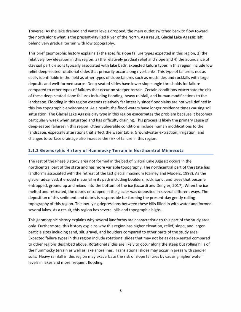
Traverse. As the lake drained and water levels dropped, the main outlet switched back to flow toward
the north along what is the present-day Red River of the North. As a result, Glacial Lake Agassiz left
behind very gradual terrain with low topography.
This brief geomorphic history explains 1) the specific slope failure types expected in this region, 2) the
relatively low elevation in this region, 3) the relatively gradual relief and slope and 4) the abundance of
clay soil particle soils typically associated with lake beds. Expected failure types in this region include low
relief deep-seated rotational slides that primarily occur along riverbanks. This type of failure is not as
easily identifiable in the field as other types of slope failures such as mudslides and rockfalls with large
deposits and well-formed scarps. Deep-seated slides have lower slope angle thresholds for failure
compared to other types of failures that occur on steeper terrain. Certain conditions exacerbate the risk
of these deep-seated slope failures including flooding, heavy rainfall, and human modifications to the
landscape. Flooding in this region extends relatively far laterally since floodplains are not well defined in
this low topographic environment. As a result, the flood waters have longer residence times causing soil
saturation. The Glacial Lake Agassiz clay type in this region exacerbates the problem because it becomes
particularly weak when saturated and has difficulty draining. This process is likely the primary cause of
deep-seated failures in this region. Other vulnerable conditions include human modifications to the
landscape, especially alterations that affect the water table. Groundwater extraction, irrigation, and
changes to surface drainage also increase the risk of failure in this region.
2.1.2 Geomorphic History of Hummocky Terrain in Northcentral Minnesota
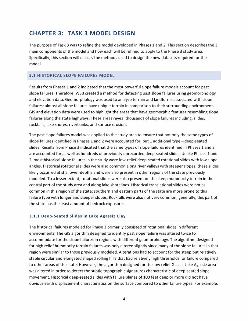
The rest of the Phase 3 study area not formed in the bed of Glacial Lake Agassiz occurs in the
northcentral part of the state and has more variable topography. The northcentral part of the state has
landforms associated with the retreat of the last glacial maximum (Carney and Mooers, 1998). As the
glacier advanced, it eroded material in its path including boulders, rock, sand, and trees that become
entrapped, ground up and mixed into the bottom of the ice (Lusardi and Dengler, 2017). When the ice
melted and retreated, the debris entrapped in the glacier was deposited in several different ways. The
deposition of this sediment and debris is responsible for forming the present-day gently rolling
topography of this region. The low-lying depressions between these hills filled in with water and formed
several lakes. As a result, this region has several hills and topographic highs.
This geomorphic history explains why several landforms are characteristic to this part of the study area
only. Furthermore, this history explains why this region has higher elevation, relief, slope, and larger
particle sizes including sand, silt, gravel, and boulders compared to other parts of the study area.
Expected failure types in this region include rotational slides that may not be as deep-seated compared
to other regions described above. Rotational slides are likely to occur along the steep but rolling hills of
the hummocky terrain as well as lake shorelines. Translational slides may occur in areas with sandier
soils. Heavy rainfall in this region may exacerbate the risk of slope failures by causing higher water
levels in lakes and more frequent flooding.
4
CHAPTER 3: TASK 3 MODEL DESIGN
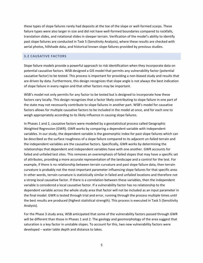
The purpose of Task 3 was to refine the model developed in Phases 1 and 2. This section describes the 3
main components of the model and how each will be refined to apply to the Phase 3 study area.
Specifically, this section will discuss the methods used to design the new datasets required for the
model.
3.1 HISTORICAL SLOPE FAILURES MODEL
Results from Phases 1 and 2 indicated that the most powerful slope failure models account for past
slope failures. Therefore, WSB created a method for detecting past slope failures using geomorphology
and elevation data. Geomorphology was used to analyze terrain and landforms associated with slope
failures; almost all slope failures have unique terrain in comparison to their surrounding environment.
GIS and elevation data were used to highlight the areas that have geomorphic features resembling slope
failures along the state highways. These areas reveal thousands of slope failures including, slides,
rockfalls, lake shores, riverbanks, and surface erosion.
The past slope failures model was applied to the study area to ensure that not only the same types of
slope failures identified in Phases 1 and 2 were accounted for, but 1 additional type—deep-seated
slides. Results from Phase 3 indicated that the same types of slope failures identified in Phases 1 and 2
are accounted for as well as hundreds of previously unrecorded deep-seated slides. Unlike Phases 1 and
2, most historical slope failures in the study were low-relief deep-seated rotational slides with low slope
angles. Historical rotational slides were also common along river valleys with steeper slopes; these slides
likely occurred at shallower depths and were also present in other regions of the state previously
modeled. To a lesser extent, rotational slides were also present on the steep hummocky terrain in the
central part of the study area and along lake shorelines. Historical translational slides were not as
common in this region of the state; southern and eastern parts of the state are more prone to this
failure type with longer and steeper slopes. Rockfalls were also not very common; generally, this part of
the state has the least amount of bedrock exposure.
3.1.1 Deep-Seated Slides in Lake Agassiz Clay
The historical failures modeled for Phase 3 primarily consisted of rotational slides in different
environments. The GIS algorithm designed to identify past slope failure was altered twice to
accommodate for the slope failures in regions with different geomorphology. The algorithm designed
for high relief hummocky terrain failures was only altered slightly since many of the slope failures in that
region were similar to those previously modeled. Alterations had to account for the steep but relatively
stable circular and elongated shaped rolling hills that had relatively high thresholds for failure compared
to other areas of the state. However, the algorithm designed for the low relief Glacial Lake Agassiz area
was altered in order to detect the subtle topographic signatures characteristic of deep-seated slope
movement. Historical deep-seated slides with failure planes of 100 feet deep or more did not have
obvious earth displacement characteristics on the surface compared to other failure types. For example,
5
these types of slope failures rarely had deposits at the toe of the slope or well-formed scarps. These
failure types were also larger in size and did not have well-formed boundaries compared to rockfalls,
translation slides, and rotational slides in steeper terrain. Verification of the model’s ability to identify
past slope failures are conducted in Task 5 (Sensitivity Analysis), where these results are checked with
aerial photos, hillshade data, and historical known slope failures provided by previous studies.
3.2 CAUSATIVE FACTORS
Slope failure models provide a powerful approach to risk identification when they incorporate data on
potential causative factors. WSB designed a GIS model that permits any vulnerability factor (potential
causative factor) to be tested. This process is important for providing a non-biased study and results that
are driven by data. Furthermore, this design recognizes that slope angle is not always the best indication
of slope failure in every region and that other factors may be important.
WSB’s model not only permits for any factor to be tested but is designed to incorporate how these
factors vary locally. This design recognizes that a factor likely contributing to slope failure in one part of
the state may not necessarily contribute to slope failures in another part. WSB’s model for causative
factors allows for multiple causative factors to be included in the model at once, and for each one to
weigh appropriately according to its likely influence in causing slope failures.
In Phases 1 and 2, causative factors were modeled by a geostatistical process called Geographic
Weighted Regression (GWR). GWR works by comparing a dependent variable with independent
variables. In our study, the dependent variable is the geomorphic index for past slope failures which can
be described as the surface roughness of a slope failure compared to its adjacent un-failed terrain and
the independent variables are the causative factors. Specifically, GWR works by determining the
relationships that dependent and independent variables have with one another. GWR accounts for
failed and unfailed test sites. This removes an overemphasis of failed slopes that may have a specific set
of attributes, providing a more accurate representation of the landscape and a control for the test. For
example, if there is no relationship between terrain curvature and past slope failure data, then terrain
curvature is probably not the most important parameter influencing slope failures for that specific area.
In other words, terrain curvature is statistically similar in failed and unfailed locations and therefore not
a strong local causative factor. If there is a correlation between these variables, then the independent
variable is considered a local causative factor. If a vulnerability factor has no relationship to the
dependent variable across the whole study area that factor will not be included as an input parameter in
the final model. GWR is tested through trial and error, running through the process multiple times until
the best results are produced (highest statistical strength). This process is executed in Task 5 (Sensitivity
Analysis).
For the Phase 3 study area, WSB anticipated that some of the vulnerability factors passed through GWR
will be different than those in Phases 1 and 2. The geology and geomorphology of the area suggest that
saturation is a key factor in unstable slopes. To account for this, two new vulnerability factors were
developed – water table depth and distance to lakes.
6
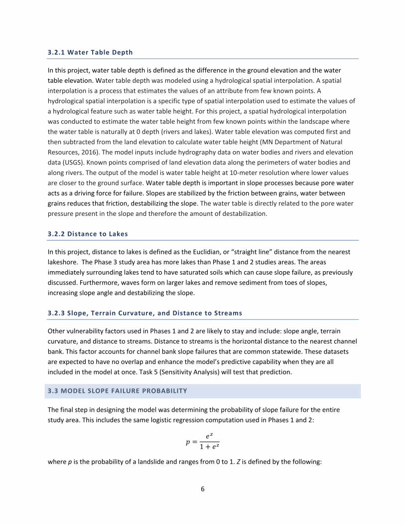
3.2.1 Water Table Depth
In this project, water table depth is defined as the difference in the ground elevation and the water
table elevation. Water table depth was modeled using a hydrological spatial interpolation. A spatial
interpolation is a process that estimates the values of an attribute from few known points. A
hydrological spatial interpolation is a specific type of spatial interpolation used to estimate the values of
a hydrological feature such as water table height. For this project, a spatial hydrological interpolation
was conducted to estimate the water table height from few known points within the landscape where
the water table is naturally at 0 depth (rivers and lakes). Water table elevation was computed first and
then subtracted from the land elevation to calculate water table height (MN Department of Natural
Resources, 2016). The model inputs include hydrography data on water bodies and rivers and elevation
data (USGS). Known points comprised of land elevation data along the perimeters of water bodies and
along rivers. The output of the model is water table height at 10-meter resolution where lower values
are closer to the ground surface. Water table depth is important in slope processes because pore water
acts as a driving force for failure. Slopes are stabilized by the friction between grains, water between
grains reduces that friction, destabilizing the slope. The water table is directly related to the pore water
pressure present in the slope and therefore the amount of destabilization.
3.2.2 Distance to Lakes
In this project, distance to lakes is defined as the Euclidian, or “straight line” distance from the nearest
lakeshore. The Phase 3 study area has more lakes than Phase 1 and 2 studies areas. The areas
immediately surrounding lakes tend to have saturated soils which can cause slope failure, as previously
discussed. Furthermore, waves form on larger lakes and remove sediment from toes of slopes,
increasing slope angle and destabilizing the slope.
3.2.3 Slope, Terrain Curvature, and Distance to Streams
Other vulnerability factors used in Phases 1 and 2 are likely to stay and include: slope angle, terrain
curvature, and distance to streams. Distance to streams is the horizontal distance to the nearest channel
bank. This factor accounts for channel bank slope failures that are common statewide. These datasets
are expected to have no overlap and enhance the model’s predictive capability when they are all
included in the model at once. Task 5 (Sensitivity Analysis) will test that prediction.
3.3 MODEL SLOPE FAILURE PROBABILITY
The final step in designing the model was determining the probability of slope failure for the entire
study area. This includes the same logistic regression computation used in Phases 1 and 2:
𝑝 =𝑒𝑧
1 + 𝑒𝑧
where p is the probability of a landslide and ranges from 0 to 1. Z is defined by the following:

7
𝑧 = 𝛽0 + 𝛽1𝑋1 + 𝛽2𝑋2 +⋯+ 𝛽𝑛𝑋𝑛
where X1,2,…,n are the independent variables, β1,2,…,n are the coefficient outputs from GWR, and β0 is the
intercept from GWR. The input parameters, test sites, and counties will change for Phase 3. This final
stage of the model incorporates data from Parts 1 and 2 – Historical Slope Failures and Causative
Factors.

8
CHAPTER 4: TASK 4 DATA COLLECTION
Task 4 of this project included data collection of the slope vulnerability factors. The data includes a
combination of publicly available data and data derived from elevation data. This project includes the
following slope vulnerability factors and their sources:
Digital Elevation Models (DEM): United States Geological Survey (USGS)
Slope angle (DEM-derived)
Terrain curvature (DEM-derived)
Proximity to streams: (Derived from DNR rivers and streams shapefile)
Distance to lakes: (Derived from DNR lakes shapefile)
Water table depth: (Derived from DNR lakes and streams shapefile and DEM)
It is important to note that in this project, vulnerability factors are all potential causative factors,
whereas input parameters are statistically tested causative factors determined in later Tasks.

9
CHAPTER 5: TASK 5 SENSITIVITY ANALYSIS
Task 5 of the slope vulnerability project included a series of tests collectively called the Sensitivity
Analysis. A sensitivity analysis determines how well the GIS model predicts slope failures and how the
model responds to changes in testing parameters.
5.1 PHASE 1 RECAP
The sensitivity analysis tested five factors:
elevation data resolution,
appropriate size of the study area (distance from road centerline),
ability of the geomorphic index to detect past failures,
testing various vulnerability factors in the model,
testing site selection for the model.
Three of these factors — elevation resolution, size of the study area, and site selection methods were
not adjusted for the Phase 3 study area and did not require further testing. However, they required
different data collection and model preparation than for Phases 1 and 2. Recap of the Phase 1 and 2
results for these factors are described below in further detail.
5.1.1 Elevation Data Resolution
Spatial data resolution is an important quality control measure that affects the predictive accuracy of
the model. The optimum level of resolution depends on the specific project objectives and scale of
study. The model objectives in this study are to locate historic slope failures, determine the causative
factors, and determine the risk of new slope failures. Elevation data at 1-meter, 3-meter, and 10-meter
resolutions were tested to determine the most efficient resolution in locating and predicting slope
failures at the district level (Holmstadt, Bradley, & Muehlbach, 2019).
In summary, the results indicated that 10-meter elevation resolution is most appropriate for the scale of
the study. Smaller resolutions are time consuming, data intensive, and may be less accurate. They detect
too much detail not required to meet project objectives and therefore do not improve model
predictions. For example, artificial slopes like landscaped hills are detected using 1 and 3-meter
resolution data. These “slopes” would need to be manually deleted from results. More information
about the elevation resolution process please see Phase 1 Slope Vulnerability final report (Holmstadt et
al., 2019).
Elevation data at 10-meter resolution was applied for the Phase 3 study area as well.
5.1.2 Appropriate Size of the Study Area
Selecting an appropriately sized study area (distance from road centerline) underpins the predictive
accuracy of the model. The area incorporated into the model must balance the amount of data
10
incorporated into the model with ensuring that the maximum number of slope failures are detected. In
Phase 1, three options were analyzed: sub-watersheds that intersect the highways, a uniform buffer of
0.5 miles on each side of the highway, and a combination of the two.
In summary, testing results indicated a 0.5-mile buffer is the most appropriately sized study area for this
project, since it captures slope failures most likely to occur in Minnesota (Holmstadt et al., 2019).
A 0.5-mile study area was applied for the Phase 3 counties as well.
5.1.3 Testing Site Selection
Determining the number of testing sites for incorporation into the model was one of the final steps of
the Phase 1 sensitivity analysis. Testing sites are a combination of verified historic slope failures and
randomly generated locations in GIS used to test the results of the sensitivity analysis and run the
model. Typically, a minimum of 30 sites are recommended for statistical analyses. For Phase 1, WSB
included over 30,000 sites (combination of verified and random) for incorporation into the model
(Holmstadt et al., 2019).
In summary, testing results indicated that the most important factor in site selection is including
locations from both failed and non-failed areas rather than the sheer number of sites because the
results of GWR will be interpolated for all areas in the study area. If only failed areas were included in
the model, the interpolated surfaces will inaccurately have high probabilities of failure.
Site selection for Phase 3 included similar methods—combination of verified and randomly generated
sites, and a combination of failed and non-failed sites. The sites are single 10 by 10-meter grid cells and
the total number of sites for Phase 3 is over 200,000, due to the larger scale of the study area. However,
the number of sites per county is roughly the same as previous phases.
5.2 PHASE 3 TESTING HISTORIC FAILURE GEOMORPHIC INDEX
5.2.1 Phase 1 and 2 Recap
WSB created a method for detecting historic slope failures by searching for geomorphic features that
resemble failed slopes using elevation data as the only input (Phases 1 and 2 Final Report). The accuracy
of this measure was compared to known slope failure sites from other work and verified with aerial
photos and hillshade data for Phases 1 and 2. In summary, thousands of slopes from Phases 1 and 2
study areas were identified as having high risk of historic slope failures. This historic slope failure model
is powerful because it accounts for over a dozen slope failure types while identifying the most common
failure type occurring in each region. For example, rockslides and falls were more common in
southeastern Minnesota, but slides along tributary ravines were more common in southwestern
Minnesota. Both slope failure types were objectively detected using the same historic slope failures
algorithm. The objective of the Phase 3 historic slope failures sensitivity analysis was to determine if the
algorithm from Phases 1 and 2 should be adjusted for the new study area.
11
5.2.2 Phase 3 Adjustments
The results from the previous Tasks of this project indicated that the historic slope failures model may
need to be adjusted in order to account for the new geomorphology and expected failure types in the
Phase 3 study area (Phase 3 Tasks 2-4 Report). The literature review identified that much of the study
area is within Glacial Lake Agassiz, which has very low relief and gradual terrain with slope failures likely
characterized by deep-seated slides. These deep-seated slides occurring beneath the land surface have
subtle topographic signatures compared to other failure types that have more obvious signs of slope
displacement on the surface (Appendix A; Figure 4). Other parts of the study area consisted of
hummocky terrain characteristic of rolling hills with more relief than Glacial Lake Agassiz, but relatively
stable slopes with shorter lengths and heights. The characteristics of these regions do not have obvious
terrain features indicating historic failures have occurred. Therefore, the geomorphic index used to
quantify topographic signatures such as past slope failures was adjusted to account for these more
subtle slope failures while also ensuring that the same failure types in Phases 1 and 2 were also
accounted.
The sensitivity analysis tested the accuracy of this adjusted historic slope failures model. As a control,
the same algorithm developed in Phases 1 and 2 was implemented for the new study area but was
expected to not fully capture the new failure types. The results show that the same algorithm
underestimated the amount of slope failures in the Glacial Lake Agassiz region and overestimated the
amount of slope failures in the region with hummocky terrain. It underestimated the slope failures in
the Glacial Lake Agassiz region because it did not detect the subtle deep-seated slope failures known to
occur along the cut banks of the Red River and its tributaries. Deep-seated slope failures in this river
valley were characteristic of having short head scarps and very little to no slide deposits or other definite
characteristics. The failures were also larger in area than typical translational or rotational slides. Some
deep-seated slides also had what appeared to look like gradual waves in the mid-section of the slides
instead of a bowl-shaped circular plane of failure. This feature is likely caused by slope movement
occurring in series perpendicular to the river’s flow. The model was adjusted to detect these subtle
scarp features associated with deep-seated slides. For example, one changed parameter was lowering
the size of the area used in detecting slope failures at any given location to more accurately pinpoint the
smaller scarps.
Conversely, the model initially overestimated the slope failures occurring in the region with hummocky
terrain because there were more features that falsely resembled slope failures. These features are part
of the natural glacial terrain and constitute the types of depositional environments left behind by
glaciers. The model was adjusted to correct for this error and to differentiate between glacially
deposited landforms and slope failure deposits. This first part of the sensitivity analysis confirmed that
the adjusted historic slope failures model was more accurate than the algorithm applied in Phases 1 and
2.
After the historic slope failure models were tested against the control, they were further tested to
determine if they accurately identified locations with known slope failures from other reports and
historic failures visible in aerial photos and hillshade data. The results from this part of the sensitivity
12
analysis indicated that the historic slope failure models accurately identified these locations with known
failures. In general, there were less slope failures recorded from other reports in this region of the state
compared to previously modeled regions. However, for the few that were previously reported, the
model accurately identified these locations as historic failures. For example, one known failure was
previously reported along a channel bank in Crookston, MN and the historic failures model accurately
identified this location. Furthermore, less slope failures were visible in aerial photos compared to
hillshade data due to the subtle nature of the failure types. Hillshade data therefore proved to be a
better check on the historic slope failures model overall for the Phase 3 study area.
5.3 PHASE 3 TESTING VULNERABILITY FACTORS
The process of statistically testing all potential causative factors of slope failures was completed in this
Task. Task 4 defined vulnerability factors as all potential causative factors, whereas input parameters are
causative factors with the greatest statistical strength. Vulnerability factors are discarded as input
parameters through a process of elimination based on statistical strength. This statistical indicator is the
r-squared value results of geographic weighted regressions (GWR) (Tasks 2-4 Report). The following
sections outline the results of this process in more detail.
5.3.1 Phase 1 Final Input Parameters
The sensitivity analysis results from Phase 1 narrowed down the number of vulnerability factors to just 4
final input parameters:
Slope angle,
Distance to streams,
Distance to bedrock outcrops, and
Terrain curvature
5.3.2 Phase 2 Final Input Parameters
The sensitivity analysis results from Phase 2 had two similar input parameters as Phase 1, but also two
new ones to account for the new geomorphology of the study area:
Slope angle
Local relief
Incision potential
Terrain curvature
5.3.3 Phase 3 Vulnerability Factors
Data on the following vulnerability factors were collected/ derived and then processed for GWR:
Slope angle – steepness of the hill
13
Terrain curvature – shape of the slope (e.g. convex or concave)
Distance to streams – horizontal distance to nearest stream bank
Distance to lakes – horizontal distance to nearest lake
Water table depth – depth to groundwater from land surface
Some datasets previously tested in Phases 1 and 2 were excluded from the sensitivity analysis of this
phase. These datasets include bedrock outcrops, stream power index, topographic wetness index,
incision potential, and local relief. They were excluded due to the model’s ability to account for the
spatial variance in these factors more efficiently with other datasets (e.g. terrain curvature and distance
to streams) or because of the absence of certain datasets in the study area (bedrock outcrops and steep
local relief).
5.3.4 Geographic Weighted Regression
As discussed in previous tasks, the execution of GWR is efficient because it not only permits more than
one causative factor to be in the model at once, but it statistically tests how these causative factors vary
locally. Furthermore, the trial and error process of GWR effectively eliminates potential causative factors
that are either weak statistically or do not enhance the model.
GWR was computed with the vulnerability factors outlined above. First, each of the vulnerability factors
were tested in the model individually, to test the accuracy of each variable in causing slope failures.
Once the variables were tested separately, different combinations of the variables were tested with the
aim of determining the best possible combination of variables that generates the greatest statistical
strength.
When the vulnerability factors are tested independently in the model the following results emerge:
Slope angle is the most important vulnerability factor with an average adjusted r-squared value of 0.650 for all 200,000 plus points across the study area (Appendix A; Table 1)
Terrain curvature is second with an average adjusted r-squared value of 0.406
Distance to streams had an average adjusted r-squared of 0.325
Water table depth had an average adjusted r-squared value of 0.312
Distance to lakes had an average adjusted r-squared value of 0.279
Water table depth had a higher than expected r-squared value, confirming that it will be incorporated as
a model input parameter. Distance to streams had a lower than expected r-squared value, indicating
that it is not the strongest predictor of slope failures. Water table elevation acts as a proxy for distance
to streams because the water table will be high close to streams. The same result occurred for distance
to lakes. Distance to lakes was expected to play a larger role in causing slope failures due to the high
prevalence of lakes in this region of the state. One possible explanation for why it does not is that
failures along lake shorelines may be better correlated with water table depth and not necessarily the
fact that a lake is nearby.

14
When different combinations of the vulnerability factors are tested in the model the following results
emerge:
Slope and terrain curvature together had an average adjusted r-squared value of 0.714
Slope and water table depth had an average adjusted r-squared value of 0.699
Slope, terrain curvature, water table depth had an average adjusted r-squared of 0.734
Slope, terrain curvature, water table depth, distance to streams had an average adjusted r-squared of 0.742
Slope, terrain curvature, water table depth, distance to streams, distance to lakes had an average adjusted r-squared of 0.739
These results highlight an important benefit of GWR — more data is not necessarily better. Additions to
the model may not enhance the results, in fact, sometimes they slightly weaken the results. This feature
minimizes the amount of data in the model and facilitates a data-driven approach for identifying
causative factors. For example, when distance to lakes is added as a fifth vulnerability factor to the
model, it lowers the average adjusted r-squared value from 0.742 to 0.739. Furthermore, other
additional vulnerability factors may slightly increase the average adjusted r-squared value only
marginally, such as distance to streams.
5.3.5 Phase 3 Final Input Parameters
The sensitivity analysis results from Phase 3 narrowed down the number of vulnerability factors to just 3
final input parameters:
Slope angle
Water table depth
Terrain curvature
The two input parameters from Phases 1 and 2—slope angle and terrain curvature—will remain in the
model. The new input parameter, water table depth, is included because it captures landforms
important for the Phase 3 study area—riverbanks, floodplains, and lake shorelines susceptible to deep-
seated failures (Appendix A; Figures 5-6).
5.4 SUMMARY
WSB tested five components of the model: resolution of spatial data, size of the study area, historic
slope failure detection, methods of site selection, and variable combinations. The sensitivity analysis
reveals that:
The geomorphic index for identifying historic failures was altered and tested to account for one
additional failure type— deep-seated failures with subtle topographic features
The most important factor in site selection is including locations from both failed and non-failed
areas

15
Statistical tests identified water table depth as the new model input parameter for Phase 3
Counties.

16
CHAPTER 6: TASK 6 DRAFT PDF MAPS AND RISK RANKING
Task 6, Produce Maps and Rank Lists was completed for 27 counties in 3 districts. In this Task, the model
was refined, scripted, and executed for the following counties: Beltrami, Clearwater, Hubbard, Kittson,
Koochiching, Lake of the Woods, Marshall, Norman, Pennington, Polk, Red Lake, Roseau (District 2);
Sherburne, Stearns, Todd, Wadena, Wright (District 3); Becker, Clay, Douglas, Grant, Mahnomen, Otter
Tail, Pope, Stevens, Traverse, and Wilkin (District 4). The deliverables include draft maps of the 27
counties, draft shapefiles, and rasters. The following sections describe the methodology and results of
this Task.
6.1 DRAFT PDF MAPS
WSB executed the model to produce slope vulnerability results. For this project, vulnerability is defined
as likelihood of failure, and risk is defined as likelihood multiplied by consequence. Figure 7 shows an
example of the draft maps and Figure 8 shows a zoomed in example of the vulnerability output
(Appendix A). The vulnerability results were then utilized in a risk ranking procedure, described in the
next section.
6.2 RISK RANKING
6.2.1 Methodology
Risk is the product of probability and consequence (Probability x Consequence = Risk); risk matrices
provide a framework for determining probability and consequence. To be most effective, risk matrices
must have robust probability and consequence definitions. The Slope Vulnerability Risk Matrix with the
definitions is presented in Appendix A Table 2.
The matrix has 4 proposed categories of risk management:
1. Site visit / action recommended,*
2. Further evaluation,*
3. Monitoring,* and
4. No further action recommended*
*Preliminary terminology for proposed risk management categories.
Definitions for the preliminary terminology are presented below:
1. Site visit / action recommended – A site specific study is recommended to determine the
best mitigation strategy for the slope.
2. Further evaluation – A site specific study is recommended to more accurately classify and
prioritize the slope.
3. Monitoring – Periodic checks on the slope are recommended.

17
4. No further action recommended – The risk is at an acceptable level and no action is
necessary for this slope at this time.
Risk ranking was conducted at the Management Area scale. Management areas are regions with similar
risk scores. This aggregates the large number of individual slopes into a workable number.
Management areas were delineated in GIS. Probability was delineated based on separating the slope
vulnerability results into 3 categories: high (p > 0.9999), medium (0.9995 < p < 0.9999), and low (p <
0.9995) likelihood of failure. Consequence was delineated based on proximity to roads and urban vs.
non-urban areas. Future field verification can further refine how to define vulnerability and
consequence.
6.2.2 Results
The draft risk rankings successfully transformed tens of thousands of slopes into hundreds of
management areas. The full list of management areas ranked by risk is presented in Table 3 of the
Appendix. The total number of areas and their total areas in square miles for each of the different
rankings are as follows:
• Action Recommended*: 370 areas (110 mi2)
• Further Evaluation*: 388 areas (56 mi2)
• Monitoring*: 456 areas (294 mi2)
• No Action*: the rest of the area of interest (3164 mi2)
The management areas range in size from a few thousand square feet to over one million square feet.
The percent of the entire domain area that each risk ranking covers is below:
• Action Recommended*: 3%
• Further Evaluation*: 1.5%
• Monitoring*: 8%
• No Action*: 87.5%
Although draft results include many management areas, the majority of the study area falls into the No
Action category.

18
CHAPTER 7: TASK 7 FIELD VERIFICATION
WSB completed Task 7 of this project—Field Verification. The objective of Task 7 was to field verify the
historic slope failure model developed in previous tasks and investigate what causative factors are
creating slope failure in the area. This task included 5 site visits—one in District 3, two in District 2, and
two in District 4. WSB chose these sites to determine the model’s capability of identifying slope failures
in different regions of the state. The following sections outline the methods, results, and conclusions of
this task.
7.1 METHODS
This section outlines the model’s progress prior to the field visits, rationale for site selection, and the
methods and equipment used during the visits.
7.1.1 Model Progress Prior to Visit
Task 7 was completed between tasks 4 and 5, in case that the model needed to be redesigned or
adjusted. Prior to the field visits, only the first part of the model was executed— Part 1 (Model Historical
Failures). Model Part 1 objectively identifies all areas of past slope failures, both where slopes are
actively failing and where slopes have previously failed but are currently more stable. Data on past slope
failures enhances predictive modeling. Predictive modeling was completed in Task 6 (Final Risk Maps).
7.1.2 Rationale for Site Selection
These sites not only had a high likelihood of past failure but are in different districts to ensure the entire
area of Phase 3 is considered in model development.
Site 1 – MN241 St. Michael, Wright County, District 3
Site 1 is located east of St. Michael, Minnesota in District 3 (Appendix A; Figure 9). It is within the
Mississippi River basin along the north side of the Crow River where a cut bank is between the river and
the road. Elevation data reveal ravines cutting up from the river to near the road.
Site 2 – MN32 Red Lake Falls, Red Lake County, District 2
Site 2 is located east of Red Lake Falls, Minnesota in District 2 (Appendix A; Figure 10). It is within the
Red River basin along the north side of the Red Lake River where the road crosses the river at a cut
bank. Lidar data show slides cutting up from the river to previously undisturbed land.
Site 3 – MN32 Red Lake Falls, Red Lake County, District 2
Site 3 is located east of Red Lake Falls, Minnesota in District 2 (Appendix A; Figure 11). It is 1.5 miles
west on MN32 from Site 2. This site was chosen because aerial photos reveal a slide on the bank of the
river, near the road.

19
Site 4 – I-94 Fergus Falls, Otter Tail County, District 4
Site 4 is located north of Fergus Falls, Minnesota in District 4 (Appendix A; Figure 12). It is within the Red
River basin where the Pelican River exits a culvert under I-94. This site was not selected beforehand,
rather the team saw a distinct headscarp from the road and decided to make an additional stop.
Site 5 – I-94 Fergus Falls, Otter Tail County, District 4
Site 5 is located west of Fergus Falls, Minnesota in District 4 (Appendix A; Figure 13). It is within the Red
River basin along the east side of the Otter Tail River where multiple cut banks near the road.
7.1.3 Equipment
The methods for this task along with equipment used are listed below:
Navigation from site to site (ESRI mobile apps and printed maps)
Quantifying slope angles using a laser range finder (Halo XL 450)
Geomorphic, geologic, and hydrologic observations (field forms and photos with Datafi web
service and iPad)
The 5 site visits were completed on November 19th and 20th, 2019.
7.2 RESULTS
The model’s capability of identifying areas at risk was validated in the field. All sites are active and are
supported with evidence from the field. The following sub-sections describe the field results in more
detail.
7.2.1 Site 1 – MN241 St. Michael, Wright County, District 3
The field results confirm that Site 1 is an active river cut bank and ravine caused by a culvert passing
below MN241 (Appendix A; Figures 14-17). The ravine has very steep walls near the river but as it as it
approaches the road, the slopes become less extreme. The nearest active erosion to the road is around
50 feet away. The slopes immediately adjacent to the road are gently sloping and highly vegetated.
Evidence of active erosion includes the following:
Headscarps along both riverbank and ravine walls
Exposed roots from soil removal
Recently fallen trees
7.2.2 Site 2 – MN32 Red Lake Falls, Red Lake County, District 2
The field results confirm that Site 2 is an active river cut bank and near where MN32 crosses the Red
Lake River (Appendix A; Figures 18-20). The riverbank has very steep walls on either side of the bridge,

20
but vegetation and human placed roughness have reduced erosion under the bridge and have kept the
slopes shallower.
Evidence of active erosion includes the following:
Steep slopes on riverbanks
Recently fallen trees
7.2.3 Site 3 – MN32 Red Lake Falls, Red Lake County, District 3
The field results confirm that Site 3 is an active river cut bank and near where MN32 crosses the Red
Lake River (Appendix A; Figures 21-22). Like Site 2, there are very steep slopes along the river on either
side of the bridge. This site has vegetation and added roughness under the bridge as well, however
there are small headscarps forming to the north side of the bridge.
Evidence of active erosion includes the following:
Headscarps along riverbank
Exposed roots from soil removal
Recently fallen trees
7.2.4 Site 4 – I-94 Fergus Falls, Otter Tail County, District 4
The field results confirm that Site 4 is an active valley wall with erosion caused by a culvert passing
below I-94 (Appendix A; Figures 23-25). South of the culvert exit is a very steep wall with evidence of
recent failure. The culvert structure is concrete, but a gully is actively forming on the southern side of it,
expanding toward the road.
Evidence of active erosion includes the following:
Headscarps along valley wall
Exposed roots from soil removal
Recently fallen trees
Exposed soil
7.2.5 Site 5 – I-94 Fergus Falls, Otter Tail County, District 4
The field results confirm multiple active river cut banks at Site 5 (Appendix A; Figures 26-28). The
northern cut bank (Site 5a) has both headscarps along it and gullies growing from the river towards the
road. The southern cut bank (Site 5b) has multiple headscarps along it and is closer to the road than the
northern cut bank. The area is highly vegetated; however, erosion is still occurring.
Evidence of active erosion includes the following:
Headscarps along both riverbank and ravine walls
Exposed roots from soil removal

21
Recently fallen trees
Gully formation
7.3 CONCLUSIONS
Field verification results suggested that the historic failures model was overestimating the number and
scale of the slope failures in the Phase 3 study area. Therefore, the model was updated by increasing the
threshold on the past failure geomorphic index and decreasing the aggregation distance for slopes.
Increasing the roughness threshold means that only areas with the highest likelihood of past failure are
considered historic slope failures. Decreasing the aggregation distance prevents separate slope failures
from being grouped together as one failure. The results of these two changes are more representative
of what was observed in the field (Appendix A; Figure 29).
22
CHAPTER 8: TASK 8 FINAL REPORT, FINAL MAPS, GIS MODEL
AND DOCUMENTATION
The deliverables in this phase include the following: draft report, final report, final PDF maps,
vulnerability raster files, the GIS model and model documentation, and the proposed management
areas ranked by risk for efficient use of project results.
8.1 FINAL PDF MAPS
WSB completed final PDF maps for the following counties: Beltrami, Clearwater, Hubbard, Kittson,
Koochiching, Lake of the Woods, Marshall, Norman, Pennington, Polk, Red Lake, and Roseau (District 2);
Sherburne, Stearns, Todd, Wadena, and Wright (District 3); and Becker, Clay, Douglas, Grant,
Mahnomen, Otter Tail, Pope, Stevens, Traverse, and Wilkin (District 4). In Phase 2, the naming
conventions of the management areas were modified. In Phase 2, management areas were labeled as
“proposed management areas” and the titles of the four categories of risk management were marked as
preliminary titles. These changes are to reflect the preliminary nature of the consequence definition and
are continued into Phase 3.
8.2 VULNERABILITY RASTER FILES
WSB combined the vulnerability final outputs from each of the 27 counties into one raster file that has
the appropriate symbology, correct size study area, and most updated roads jurisdiction. The file is
readily available for use in any ArcGIS platform.
8.3 PROPOSED MANAGEMENT AREAS SHAPEFILES
WSB combined the proposed management areas final outputs from each of the 27 counties into one
shapefile that has the appropriate symbology, correct size of study area, and most updated roads
jurisdiction. The file is readily available for use in any ArcGIS platform.
8.4 GIS MODEL AND DOCUMENTATION
WSB provided MnDOT the GIS model along with appropriate scripts and documentation for running the
model. Final scripting edits included clipping the final outputs to a half-mile buffer and ensuring every
cell within the study area had a value. When running the model, MnDOT will be prompted with
instructions on how to use it.
8.5 RECOMMENDED NEXT STEPS
The results of this study are intended to be the first step of actions required in minimizing the effects of
slope failure including expensive mitigation actions and threats to public safety. In this study, the GIS
model developed in previous phases was refined and implemented to identify slope vulnerability along
state trunk highways for 27 more counties. The model’s capability of identifying slope vulnerability

23
anywhere in the Phase 3 study area with minimal data input was field verified. Final maps depicting
slope vulnerability for 27 counties in 4 districts were produced and proposed management areas were
ranked based on risk that can provide useful information for district, county, or city engineers, planners,
project managers, and maintenance staff. Several steps should be taken to maximize the value and
usefulness of the model:
Complete a robust risk estimation that incorporates the geomorphic vulnerabilities evaluated in this study with consequence definitions that will guide further action
Field verification of the 370 sites with action recommended
Incorporate the risk factors determined in this project into MnDOT’s TAMP
Design and implement mitigation and monitoring programs including severe weather investigations
Model and produce results for other districts within the state (Phase 4)
24
REFERENCES
Camey, L. M., & Mooers, H. D. (1998). Landform assemblages and glacial history of a portion of the
Itasca moraine, north-central Minnesota. St. Paul, MN: University of Minnesota.
DNR. (2016). Methods for estimating water-table elevation and depth to water table: Minnesota
Department of Natural Resources (GW-04). St. Paul, MN: Minnesota Department of Natural
Resources.
Holmstadt, J., Bradley, N., & Muehlbach, P. (2019). MnDOT Slope Vulnerability Assessments (No. MN/RC
2019-12). St. Paul, MN: Minnesota Department of Transportation.
Leverington, D. W., Mann, J. D., & Teller, J. T. (2000). Changes in the bathymetry and volume of glacial
Lake Agassiz between 11,000 and 9300 14 C yr BP. Quaternary Research, 54(2), 174–181.
Lusardi, B. A., & Dengler, E. L. (2017). Minnesota at a glance quaternary glacial geology. St. Paul, MN:
Minnesota Geological Survey.
Teller, J. T., Leverington, D. W., & Mann, J. D. (2002). Freshwater outbursts to the oceans from glacial
Lake Agassiz and their role in climate change during the last deglaciation. Quaternary Science
Reviews, 21(8-9), 879–887.